| Issue |
A&A
Volume 703, November 2025
|
|
|---|---|---|
| Article Number | A103 | |
| Number of page(s) | 19 | |
| Section | Extragalactic astronomy | |
| DOI | https://doi.org/10.1051/0004-6361/202556427 | |
| Published online | 18 November 2025 | |
Polycyclic aromatic hydrocarbon destruction in star-forming regions across 42 nearby galaxies
1
Astronomisches Rechen-Institut, Zentrum für Astronomie der Universität Heidelberg, Mönchhofstraße 12-14, D-69120 Heidelberg, Germany
2
Department of Astronomy, The Ohio State University, 140 West 18th Avenue, Columbus, Ohio 43210, USA
3
Center for Cosmology and Astroparticle Physics, 191 West Woodruff Avenue, Columbus, OH 43210, USA
4
Department of Astronomy & Astrophysics, University of California, San Diego, 9500 Gilman Drive, La Jolla, CA 92093, USA
5
Kavli Institute for Particle Astrophysics & Cosmology, Stanford University, CA, 94305, USA
6
Center for Decoding the Universe, Stanford University, CA, 94305, USA
7
INAF – Osservatorio Astrofisico di Arcetri, Largo E. Fermi 5, I-50157 Firenze, Italy
8
Whitman College, 345 Boyer Avenue, Walla Walla, WA 99362, USA
9
Université Côte d’Azur, Observatoire de la Côte d’Azur, CNRS, Laboratoire Lagrange, 06000 Nice, France
10
Dr. Karl-Remeis Sternwarte and Erlangen Centre for Astroparticle Physics, Friedrich-Alexander Universitat Erlangen-Nurnberg, Sternwartstr. 7, 96049 Bamberg, Germany
11
European Southern Observatory (ESO), Alonso de Córdova 3107, Casilla 19, Santiago 19001, Chile
12
Department of Physics and Astronomy, University of Wyoming, Laramie, WY 82071, USA
13
Sub-department of Astrophysics, Department of Physics, University of Oxford, Keble Road, Oxford OX1 3RH, UK
14
Sterrenkundig Observatorium, Universiteit Gent, Krijgslaan 281 S9, B-9000 Gent, Belgium
15
Institute of Astronomy and Astrophysics, Academia Sinica, No. 1, Sec. 4, Roosevelt Road, Taipei 106319, Taiwan
16
Department of Physics, University of Alberta, Edmonton, AB T6G 2E1, Canada
17
International Gemini Observatory, NSF NOIRLab, 950 N Cherry Ave, Tucson, AZ 85719, USA
18
Space Telescope Science Institute, 3700 San Martin Drive, Baltimore, MD 21218, USA
19
Instituto de Astronomía, Universidad Nacional Autónoma de México, Ap. 70-264, 04510 CDMX, Mexico
20
Department of Physics,Tamkang University, No.151, Yingzhuan Rd., Tamsui Dist., New Taipei City 251301, Taiwan
21
Max-Planck-Institutfür Astronomie, Künigstuhl 17, D-69117 Heidelberg, Germany
22
Department of Physics and Astronomy,The Johns Hopkins University, Baltimore, MD 21218, USA
⋆ Corresponding author: This email address is being protected from spambots. You need JavaScript enabled to view it.
Received:
15
July
2025
Accepted:
17
September
2025
Abstract
Polycyclic aromatic hydrocarbons (PAHs) are widespread in the interstellar medium (ISM) of near solar metallicity galaxies, where they play a critical role in ISM heating, cooling, and reprocessing stellar radiation. The PAH fraction, the abundance of PAHs relative to total dust mass, is a key parameter in ISM physics. Using JWST and MUSE observations of 42 galaxies from the PHANGS survey, we analyzed the PAH fraction in over 17 000 H II regions spanning a gas-phase oxygen abundance of 12 + log(O/H) = 8.0–8.8 (Z ∼ 0.2–1.3 Z⊙), and ∼400 isolated supernova remnants (SNRs). We find a significantly lower PAH fraction toward H II regions compared to a reference sample of diffuse ISM areas at matched metallicity. At 12 + log(O/H) > 8.2, the PAH fraction toward H II regions is strongly anti-correlated with the local ionization parameter, suggesting that PAH destruction is correlated with ionized gas and/or hydrogen-ionizing UV radiation. At lower metallicities, the PAH fraction declines steeply in H II regions and in the diffuse ISM, likely reflecting less efficient PAH formation in metal-poor environments. Carefully isolating dust emission from the vicinity of optically identified supernova remnants, we see evidence of selective PAH destruction from measurements of lower PAH fractions, which is, however, indistinguishable at ∼50 pc scales. Overall, our results point to ionizing radiation as the dominant agent of PAH destruction within H II regions; metallicity plays a key role in their global abundance in galaxies.
Key words: ISM: abundances / dust / extinction / HII regions / galaxies: ISM / infrared: ISM
© The Authors 2025
 Open Access article, published by EDP Sciences, under the terms of the Creative Commons Attribution License (https://creativecommons.org/licenses/by/4.0), which permits unrestricted use, distribution, and reproduction in any medium, provided the original work is properly cited.
This article is published in open access under the Subscribe to Open model. This email address is being protected from spambots. You need JavaScript enabled to view it. to support open access publication.
1. Introduction
Polycyclic aromatic hydrocarbons (PAHs) are carbon-based nanoparticles that are ubiquitous in the interstellar medium (ISM). Together with stochastically heated very small dust grains (20 − 30 Å), PAHs are dominant contributors to the mid-infrared (mid-IR) spectra of galaxies (e.g. Draine & Li 2007). PAHs absorb ultraviolet (UV) and optical photons and re-emit energy in the IR range in the form of continuum emission and several strong emission features at 3.3, 6.2, 7.7, 8.6, 11.3, 12.7, and 17 μm (Tielens 2008; Li 2020). As a result, PAHs are responsible for reprocessing up to 20% of all stellar UV/optical radiation (Smith et al. 2007). Observationally, PAHs are considered good tracers of both cold gas (Gao et al. 2019, 2022; Leroy et al. 2023; Sandstrom et al. 2023b; Whitcomb et al. 2023; Chown et al. 2025b) and heating processes, due to their association with star formation activity (Peeters et al. 2004; Calzetti et al. 2007; Calapa et al. 2014; Cluver et al. 2017; Pathak et al. 2024; Gregg et al. 2024).
Polycyclic aromatic hydrocarbons are important for the evolution of the ISM and star formation in galaxies; they provide shielding from UV radiation and dominate photoelectric heating in neutral gas (Wolfire et al. 1995, 2003; Li 2020; Draine et al. 2021), and thus influence how much gas is available to form molecular clouds. Meanwhile, the mechanisms of their formation and destruction are not fully understood. Possible scenarios include PAH formation in the atmospheres of evolved stars (e.g., Latter 1991; Cherchneff et al. 1992) or directly in molecular clouds (e.g., Greenberg et al. 2000; Sandstrom et al. 2010; Chastenet et al. 2019; Burkhardt et al. 2021; McGuire et al. 2021) via the shattering of larger dust grains (e.g., Jones et al. 1996; Hirashita & Yan 2009; Seok et al. 2014; Wiebe et al. 2014). Ionization and photodestruction by hard UV radiation (e.g., Allain et al. 1996; Montillaud et al. 2013; Pavlyuchenkov et al. 2013; Wenzel et al. 2020; Egorov et al. 2023), sputtering and fragmentation in the ionized gas (Micelotta et al. 2010a; Bocchio et al. 2012), and shocks (O’Halloran et al. 2006; Jackson et al. 2006; Micelotta et al. 2010b; Zhang et al. 2022) are the main mechanisms considered for PAH destruction.
Observations of nearby galaxies suggest that the fraction of the total dust mass in PAHs, qPAH, remains relatively constant across their diffuse ISM, with a typical value of qPAH ∼ 5% for the Milky Way and near solar metallicity conditions (e.g., Draine et al. 2007; Chastenet et al. 2019; Aniano et al. 2020; Sutter et al. 2024). However, a prominent decrease in tracers of qPAH is typically observed toward H II regions (Helou et al. 2004; Relaño & Kennicutt 2009; Anderson et al. 2014; Chastenet et al. 2019, 2023a; Egorov et al. 2023; Pedrini et al. 2024; Sutter et al. 2024).
Resolved and unresolved studies of low-metallicity galaxies show a deficit of PAHs in their ISM. Such a decrease in the PAH fraction in a low-metallicity environment is typically explained through the effects of harder ionizing radiation or more ubiquitous supernova shocks efficiently destroying PAHs at lower metallicities, or that the deficiency of cold dense gas and gas-phase carbon prevents PAH formation under such conditions (e.g., Engelbracht et al. 2005, 2008; Madden et al. 2006; Draine et al. 2007; Galliano et al. 2008; Khramtsova et al. 2013; Rémy-Ruyer et al. 2015; Whitcomb et al. 2024).
Analyzing PAHs and their connection to local ISM conditions and ionizing sources in a large and representative sample of resolved star-forming regions is a key to understanding the mechanisms of their formation and destruction. Multiwavelength observations of star-forming regions with high spatial resolution (< 100 pc scales) sufficient to isolate individual H II regions and associated photodissociation regions (PDRs) from the surrounding diffuse ISM and other H II regions are crucial in order to disentangle the local and global effects on the PAH evolution. Before launching JWST, such resolved studies of PAHs were only possible in our Galaxy (e.g., Povich et al. 2007; Anderson et al. 2014; Binder & Povich 2018) and in a handful of very nearby galaxies (e.g., Bolatto et al. 2007; Sandstrom et al. 2010; Wiebe et al. 2011; Lebouteiller et al. 2011; Chastenet et al. 2017, 2019; Maragkoudakis et al. 2018; Mallory et al. 2022). JWST observations now enable investigations of PAHs toward individual H II regions, supernova remnants (SNRs), star clusters and their immediate surroundings in relatively distant galaxies (e.g., Dale et al. 2023; Egorov et al. 2023; Sutter et al. 2024; Chastenet et al. 2023a; Sandstrom et al. 2023a; Pedrini et al. 2024; Gregg et al. 2024; Baron et al. 2024, 2025; Ujjwal et al. 2024), or in unresolved star-forming regions in galaxies at redshifts up to z ∼ 2 (Shivaei et al. 2024).
Using the JWST images and MUSE integral-field spectroscopic (IFS) observations for four galaxies from the Physics at High Angular Resolution in Nearby Galaxies Survey (PHANGS; Leroy et al. 2021), Egorov et al. (2023) investigated the mechanisms of PAH destruction in ∼1500 high-metallicity H II regions. In that study they found that the PAH fraction toward the H II regions is tightly correlated with the ionization parameter. They suggested that this might indicate that the PAH destruction in the H II regions is regulated by hydrogen-ionizing radiation. For this paper we extended the analysis from Egorov et al. (2023) to all 42 PHANGS-JWST galaxies with available MUSE data (from either PHANGS or archival observations) providing us with a sample of ∼17 200 H II regions with oxygen abundance (a proxy for gas-phase metallicities) spanning a range of 12 + log(O/H) = 8.0 − 8.8 (Z = 0.2 − 1.3 Z⊙), with a few regions outside this range. This contains a large sample of ∼5600 marginally resolved (most luminous) H II regions for which we can minimize the contamination by diffuse ISM. We also extended the analysis to a sample of more than 400 isolated SNRs from the Li et al. (2024) catalog. The result is by far the largest systematic measurement of band ratios tracing the PAH fraction in spectroscopically characterized ionized nebulae. With these samples, we investigated the role of ionizing radiation and shocks in selective destruction of PAHs and how the effects of the relevant physical processes change with metallicity.
The paper is organized as follows. In Section 2 we describe the underlying observational data. Section 3 provides details on the methods and criteria implemented for selection of the H II regions and deriving the properties of gas, dust, and young stars there. Section 4 describes results from the comparison of our tracer for the PAH fraction and properties of the H II regions and SNRs. In Section 5 we discuss these results and consider the potential observational biases in this study. Section 6 summarizes our results.
2. Observations
2.1. JWST
We use the JWST data obtained in Cycle 1 and Cycle 2 as part of the PHANGS-JWST survey (programs GO 02107; PI: J. C. Lee and GO 03707; PI: A. Leroy). In Cycle 1, 19 nearby star-forming galaxies were imaged with the NIRCam (with F200W, F300M, F335M and F360M filters) and the MIRI (F770W, F1000W, F1130W and F2100W) instruments. The first public data release and the description of the data reduction process are presented in Williams et al. (2024) (see also Lee et al. 2023). In Cycle 2, 55 additional galaxies from the PHANGS survey were observed with a modified filter set: F150W, F187N (replaced by F200W for a few galaxies with higher systemic velocities), F300M, F355M for NIRCam, and F770W, F2100W for MIRI. Chown et al. (2025b) describe the basic observational setup and processing of this Cycle 2 survey. Data reduction for all objects from both Cycle 1 and Cycle 2 is done in a uniform way with the package PJPIPE1, which is described in Williams et al. (2024) and is based on the official JWST pipeline (Bushouse et al. 2023). In this paper, we use the F770W, F1130W, F2100W, and F300M images (including the associated uncertainties maps) for all 19 galaxies from Cycle 1, and F770W, F2100W, and F300M images for 23 galaxies from Cycle 2 (see Table 1). These 23 galaxies were selected from the entire sample of Cycle 2 galaxies because they have available MUSE data and derived products of quality similar to that of the PHANGS-MUSE data (Emsellem et al. 2022), which overlap with the 19 Cycle 1 PHANGS-JWST targets (see Sec. 2.2).
Properties of the galaxies.
We convolved all the images to the PSF of the F2100W images (FWHM ≃ 0.67″, corresponding to 28–64 pc at the distance of our targets), as produced by the STPSF (Perrin et al. 2014) modeling tool2. The convolution kernels were created following the procedure from Aniano et al. (2011). We note that our analysis relies on the integrated measurements within footprints of the H II regions (see Sec. 3), and therefore the exact angular resolution of the data (both the JWST and MUSE datasets) is not critical for the analysis.
2.2. MUSE
All 42 galaxies in our study were previously observed with the optical integral field spectrograph MUSE (VLT). The PHANGS-MUSE large program (1100.B-0651, PI: Schinnerer) provided data for 19 galaxies from PHANGS-JWST Cycle 1 with a coverage up to 2 effective radii for all targets, which is in general consistent with the footprint of JWST observations. The other 23 galaxies (hereafter extended sample) were observed within several complementary programs, or recovered from the ESO archive (see Table 1). Due to the heterogeneity of the extended sample, MUSE covers only a small (typically – central) part of the JWST footprint for about half of these galaxies, while the coverage of the other half of the extended sample is comparable to that of PHANGS-MUSE galaxies.
The typical angular resolution of the MUSE data in this study is ∼1″ (45–95 pc), which is sufficient to isolate individual H II regions from each other and minimize contribution from the surrounding diffuse ionized gas (Congiu et al. 2023). The MUSE data span the spectral range 4800 − 9200 Å and include several strong emission lines (Hα, Hβ, [O III] 4959, 5007 Å, [S II] 6717, 6731 Å, [N II] 6548, 6584 Å, [S III] 9069 Å) that are used in the current work.
The reduced data for the PHANGS-MUSE large program are publicly available3, and details of the observations and data reduction are given in Emsellem et al. (2022). The data for galaxies from the extended sample are reduced and analyzed in a similar way as for the main PHANGS-MUSE sample. That is, we used the Python package PYMUSEPIPE4 to produce data cubes from the raw data. PYMUSEPIPE is a wrapper around the MUSE data processing pipeline software (Weilbacher et al. 2020) and we adopted it since it allows for efficient mosaicking of multiple data cubes. For data analysis (i.e., producing the maps in emission lines by fitting the simple stellar population templates and single-component Gaussians to the observed spectra), we used the PHANGS data analysis pipeline DAP5, which relies on the GIST code (Bittner et al. 2019). Both PYMUSEPIPE and DAP are described in detail in Emsellem et al. (2022). A detailed description of the data reduction, as well as presentation of the data for the 23 galaxies from the extended sample, will be presented in future work.
3. Analysis
In this work, we investigate how the PAH fraction changes in the presence of ionized gas in and around star-forming regions. The analysis consists of four main steps: (1) identifying H II regions and SNRs in the MUSE data; (2) Reprojecting the spatial masks defining the borders of these nebulae onto the JWST grid to isolate the regions affected by ionizing radiation or SNR shocks from the diffuse ISM; (3) Measuring observational and physical properties of the ionized nebulae based on the integrated MUSE spectra of the regions; (4) Deriving JWST band ratios sensitive to the PAH mass fraction from the fluxes integrated in the apertures corresponding to the ionized nebulae or diffuse ISM. Our measurements are reported in the online catalog described in Appendix D.
3.1. Identifying H II regions and measuring the properties of the ionized gas
Following the same approach as in Egorov et al. (2023), we selected H II regions in JWST images based on the masks derived from the MUSE data using the package HIIPHOT (Thilker et al. 2000). The procedure is described in detail by Groves et al. (2023) where these masks and the corresponding nebular catalog are presented for 19 PHANGS-MUSE galaxies. The catalog contains measurements of emission line fluxes for each nebula from their integrated spectra (within the borders defined by HIIPHOT). The line fluxes are corrected for extinction based on the observed Balmer decrement. No correction for the contribution of the surrounding diffuse emission was applied. We also use measurements of the gas phase oxygen abundance (as a proxy for the metallicity), 12 + log(O/H), and circularized radii of the nebulae, rcirc, taken from the Groves et al. (2023) catalog for each H II region, or measured here in a similar way for the extended sample. The oxygen abundance was derived from the integrated emission spectra made using the strong emission line calibration “Scal” from Pilyugin & Grebel (2016), which relies on the measurements of Hβ, Hα, [O III]λ5007, [N II]λ6584 and [S II]λ6717,6731 emission lines and is usually consistent with the measurements made using the “direct” Te method (e.g., Brazzini et al. 2024). This calibration adopts 12 + log(O/H) = 8.69 (Asplund et al. 2009) as a reference value for the solar oxygen abundance.
The Groves et al. (2023) catalog contains properties of the ionized nebulae for all 19 PHANGS-MUSE galaxies. Here we analyze also the new MUSE data for 23 other galaxies from the extended sample, which were observed with JWST in Cycle 2. For these galaxies, we analyzed the MUSE data, produced the ionized nebulae spatial masks and the nebular catalog with the measured emission lines, metallicity etc. in the same way as described in Groves et al. (2023) and summarized above. Similarly to Groves et al. (2023), we classified a nebula as H II region based on its position on the diagnostic BPT diagram (Baldwin et al. 1981). We use the H II region spatial masks and derived properties of the nebulae in the remaining analysis. The new catalogs for the extended sample will be published separately in future papers.
The spatial masks for each H II region were reprojected onto the grid of the JWST/MIRI F2100W images. Given that our original MUSE data typically have coarser resolution than F2100W images, we can expect that some of the pixels in the JWST images falling into the nebular masks in fact correspond to the surrounding PDRs and diffuse ISM heated by the H II regions or even by the interstellar radiation field (ISRF). Moreover, the MUSE resolution is not sufficient for reliable measurements of the sizes of H II regions (which are typically smaller than the PSF of our MUSE data). The derived sizes are systematically overestimated by a factor of 3 compared to what is measured from the better resolution HST Hα images ((Barnes et al. 2022, 2025)). Therefore, we expect that reprojected spatial masks on the JWST / MIRI F2100W grid isolate H II regions from each other well, but have a non-negligible contribution of diffuse ISM. This contribution is expected to be higher in the case of the faint (hence small) H II regions, and closer to negligible for the luminous (and thus larger) H II regions. This is further discussed in Sec. 4.2. To minimize contamination by diffuse ISM, we also consider separately in the following analysis the subsample of the marginally resolved (luminous) H II regions, which have size exceeding 2 PSF of MUSE data (i.e., rcirc > FWHMPSF). This mostly corresponds to the extinction-corrected Hα luminosities L(Hα) > 1037 erg s−1.
We excluded from further analysis all the H II regions residing in the galactic centers, as star-forming regions in such locations are typically very crowded and the MUSE resolution does not allow us to reliably separate them from each other. Furthermore, the gas and dust excitation there can be strongly affected by processes different from what is observed in normal star-forming regions in galactic disks (e.g., active galactic nuclei (AGNs), nuclear starbursts, large-scale shocks due in the circumnuclear rings etc.). Recent studies in fact reveal destruction of PAHs by shocks and anomalous PAH-to-CO and PAH band ratios in the central regions of galaxies (e.g., Zhang et al. 2022; Chown et al. 2025b; Pathak et al. 2024; Baron et al. 2025). To exclude central regions, we used environmental masks from Querejeta et al. (2021). These masks were created with the Spitzer 3.6 μm images and distinguish between different environments in each galaxy in our sample. Therefore, our results presented below are valid for normal star-forming regions outside the galactic centers. For three galaxies that do not have published environmental masks, we applied elliptical masks derived by eye based on the Spitzer 3.6 μm (for NGC 1808) or JWST NIRCAM/F330M (for NGC 1068, NGC 3368) images to exclude the central and bar regions from the analysis.
Finally, we consider here only those H II regions with signal-to-noise ratio exceeding 10 in all important emission lines and JWST bands (i.e., [S III]λ9069 Å, [S II]λ6717,6731 Å, F770W, F1130W, F2100W) in their integrated spectra or photometry. In total, we analyze a sample of 17151 H II regions. The number of the selected H II regions for each galaxy is given in Table 1.
In this study, we rely on the reddening-corrected [S III]λ9069, 9532 Å/[S II]λ6717,6731 Å line ratio as a proxy for the ionization parameter, commonly defined as the ratio of the number densities of ionizing photons and hydrogen atoms (e.g., Diaz et al. 1991; Kewley et al. 2019; Mingozzi et al. 2020, see also Appendix C). The emission line [S III]λ9532 Å resides beyond the MUSE wavelength range. Therefore, we use the well-defined theoretical ratio between these lines: [S III]λ9532 Å = 2.5× [S III]λ9069 Å. Hereinafter, [S II] and [S III] refers to the sum of the corresponding doublets, unless otherwise specified.
3.2. Identifying SNRs and measuring their properties
We aim here to analyze how the PAH fraction in star-forming regions is affected not only by ionizing radiation, but also by shocks. We study this by measuring the PAH fraction toward the sample of SNRs identified in 19 galaxies from our sample. Li et al. (2024) found 1166 SNRs in 19 PHANGS-MUSE galaxies (outside their central parts) based on the combination of several indicators (different shock-sensitive line ratios and gas velocity dispersion). Their sample includes 964 objects isolated from any H II region, as compared with the same Groves et al. (2023) H II region catalog used in our work. We therefore consider this sample of isolated SNRs as the sites where the supernova shocks may dominate over photoionization in its influence on the dust and PAHs in the ISM. We integrated the optical spectra and fluxes in JWST bands in circular apertures with 50 pc diameter6 and analyzed them in the same way as for H II regions above to recover emission line fluxes and JWST photometry. Note that the Scal empirical metallicity calibration is not valid for the regions dominated by shocks. Therefore, similarly to Li et al. (2024), we took the values corresponding to the SNR locations from the spatially interpolated 2D metallicity maps derived by Williams et al. (2022) based on Scal measurements for the H II regions.
After excluding SNRs outside the JWST footprint and applying the same signal-to-noise criteria as for the H II regions (i.e., S/N > 10 in all emission lines and JWST bands significant for our analysis), we proceed with a sample of 398 isolated SNRs in 19 PHANGS-MUSE galaxies spanning metallicity range of 12 + log(O/H) = 8.19 − 8.63.
3.3. Tracing PAH-to-dust mass fraction
Measurement of the mass fraction of PAHs in dust, qPAH, requires SED modeling from mid- to far-IR wavelengths. Previous studies have shown that the ratio of intensity in filters dominated by PAH emission to those dominated by the small dust grain continuum can be a good observational tracer of qPAH (e.g., Engelbracht et al. 2008; Marble et al. 2010; Sandstrom et al. 2010; Sutter et al. 2024; Chastenet et al. 2025). For example, Spitzer studies relied on the F8 μm/F24 μm (i.e., IRAC4/MIPS24) band ratio as a tracer of qPAH. With JWST it is possible to use several bands sensitive to different sizes and ionization states of PAHs (e.g., 7.7 μm and 11.3 μm). Following previous works (Egorov et al. 2023; Chastenet et al. 2023a; Sutter et al. 2024), we use RPAH ≡ (F770Wss + F1130W)/F2100W as a tracer of qPAH. The measurements in corresponding JWST filters here are flux densities in MJy sr−1. Based on theoretical modeling and observations of 7 galaxies, Sutter et al. (2024) demonstrated that RPAH correlates with qPAH in cases where full far-IR coverage is available. For reference, RPAH ∼ 4 corresponds to qPAH ∼ 5%, according to their paper.
In this definition of RPAH, F770Wss corresponds to flux density of the non-stellar emission in the F770W band, i.e., to the total flux density measured in this band corrected for the contribution from stellar continuum. Stellar populations produce non-zero continuum emission at the wavelength around 8 μm (e.g., Helou et al. 2004; Marble et al. 2010; Sutter et al. 2024), and its removal is required for proper measurements of RPAH in areas of high stellar surface density and low gas density. This correction is very minor in gas-rich and dust-rich regions (∼1%; Baron et al. 2025), such as the star-forming regions considered here. Therefore, no significant differences are expected in RPAH compared to previous measurements where such a correction was not implemented (Egorov et al. 2023; Chastenet et al. 2023a). In diffuse gas, especially toward galaxy centers where the starlight is concentrated, the starlight continuum contributes more, resulting in a higher correction, typically 10 − 30% (Baron et al. 2025). The more extreme values (up to 75%) are observed only in star formation deserts, which are not considered in this work. We calculate the starlight contribution based on the NIRCam F300M images convolved at the MIRI F770W resolution as described in Sutter et al. (2024): F770Wss = F770W − (0.22 ± 0.08)×F300M. The resulting F770Wss are further convolved at the F2100W, as was described earlier in Sec. 2.1.
The fluxes measured in apertures corresponding to H II regions and SNRs are contaminated by diffuse ISM not only due to the imperfect isolation of the fainter (smaller) regions (as mentioned in Sec. 3.1), but also due to the contribution of background or foreground emission. Careful subtraction of this component is challenging due to its inhomogeneity, but necessary for analysis of the compact sources (such as SNRs) where its contribution can dominate the total flux measured in the aperture. To perform such a correction, we measured the median brightness in each photometric band in circular annuli with inner and outer radii 1.5 × rcirc and 3 × rcirc, respectively, and centered on the H II region or SNR. For SNRs, we assumed constant rcirc = 50 pc. Before measuring the median brightness, we masked all pixels that reside within H II region masks. The uncertainties of the background measurements, calculated as the standard deviation within the apertures, were propagated to the estimates of RPAH. The effect of background correction on the measured fluxes and derived RPAH is investigated in the Appendix A and Sec. 5.3. The local background does not significantly affect our measurements for H II regions, and therefore for further analysis we use mostly original, non-corrected values. However, we consider background-subtracted fluxes investigating the effect of SNRs and in some additional applications where such correction is essential.
The measurements of RPAH described here require images in the F1130W band, which are not available for 23 galaxies from Cycle 2. Meanwhile, the ratios of individual PAH-sensitive bands to the dust continuum (i.e., F770W/F2100W or F1130W/F2100W, which are similar to the previously widely used Spitzer IRAC4/MIPS24 and WISE W3/W4 ratios) were also shown to be good tracers of PAH fraction. Thus, Sutter et al. (2024) showed that RPAH* = 2.57 × F770Wss/F2100W is generally equal to RPAH for diffuse ISM if there are no significant variations in PAH charge or hardness of the interstellar radiation field expected. Based on our measurements for 19 galaxies where both F770W and F1130W, we consider in Appendix B whether RPAH* measured this way agrees well with RPAH for H II regions. We find that F770Wss/F1130W ratio grows with the Hα luminosity of a region (Fig. A.1; see also Belfiore et al. 2023), which is likely related to the differences in ratio between the ionized and neutral PAHs, or in the hardness of the radiation field (Chastenet et al. 2023b; Baron et al. 2025). In turn, this leads to a systematically higher RPAH* (by ∼7 − 17%) than RPAH in bright star-forming regions (Fig. B.1). We demonstrate that this offset can be removed with a small correction non-linearly depending on F770Wss brightness. Therefore, here we use the parameterization of
 (1)
(1)
where
 (2)
(2)
where Lν(F770Wss) is the monochromatic luminosity of the non-stellar emission in the F770W band. The latter is measured in erg s−1 Hz−1 calculated from flux density F770Wss (converted from MJy to erg s−1 cm−2 Hz−1), and distance to the galaxy D (converted to cm) as Lν(F770Wss) = 4πD2 × F770Wss. The resulting parameterization shows a better agreement with RPAH for relatively bright H II regions than the one from Sutter et al. (2024) and is in good agreement with it for the low-luminosity end. The best fit for the background-subtracted measurements slightly differs leading to a nearly constant factor correction (see Fig. B.2):
 (3)
(3)
assuming that all fluxes here and in Eq. (1) are background-subtracted.
For further analysis, we consider RPAH* derived from Eqs. (1, 2) as the reliable tracer of PAH fraction across all 42 galaxies in our sample. When considering only the 19 PHANGS-JWST galaxies from our Cycle 1 program, we rely on RPAH instead to avoid unnecessary empirical correction.
4. Results
4.1. Metallicity dependence of the PAH fraction
Previous studies of star-forming regions and galaxies at kpc-scales with Spitzer and WISE demonstrated that the PAH fraction rapidly decreases in the low-metallicity regime (e.g., Engelbracht et al. 2005; Madden et al. 2006; Draine et al. 2007; Galliano et al. 2008; Khramtsova et al. 2013; Rémy-Ruyer et al. 2015; Whitcomb et al. 2024). This is further supported by a still scarce number of resolved studies of nearby low-metallicity dwarf galaxies measuring the PAH fraction to be much lower than in the more massive galaxies (e.g., Chastenet et al. 2019; Chown et al. 2025a). These studies find a threshold between the low- and high-metallicity regimes (typically at 12 + log(O/H)∼8.0 − 8.3, although some studies report higher value; see Section 5.1), with a particularly large scatter of the PAH fraction around these values. All of these studies argue that gas-phase metallicity (or something associated with it) is among the key factors regulating the PAH life cycle, although the exact transition threshold, the particular form of the metallicity dependence, and the role of different physical mechanisms responsible for these remain uncertain.
Fig. 1 shows how log(RPAH*) changes with metallicity for our sample of 17151 H II regions spanning the metallicities 12 + log(O/H)∼8.0 − 8.8 (Z ∼ 0.2 − 1.3 Z⊙). The average values per O/H bin clearly demonstrate a drop of RPAH* at metallicities 12 + log(O/H) < 8.2 and a high-metallicity plateau. This trend is in very good agreement with the estimates for low-metallicity dwarf galaxies WLM and NGC 6822 (shown by black squares) derived as 2.57 × F770W/F2100W based on the average band ratios reported by Chown et al. (2025a), despite the slightly different treatment of the stellar continuum subtraction and calculation of RPAH*.
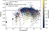 |
Fig. 1. Distribution of log(RPAH*) vs. oxygen abundance color-coded by log([SIII]/[SII]) (tracer of the ionization parameter) for all H II regions in the sample. The red circles show the average values in different metallicity bins (reported in Table 2). The vertical gray dashed line marks 12 + log(O/H) = 8.2 as a threshold between the low- and high-metallicity regimes. The horizontal dashed line corresponds to the average RPAH for diffuse ISM measured by Sutter et al. (2024). The black squares correspond to measurements for WLM and NGC6822 (from low- to high-metallicity) made by (Chown et al. 2025a) using JWST F770W and F2100W images. The PAH fraction drops significantly in the low-metallicity regime. |
The high-metallicity plateau in Fig. 1 exhibits a large scatter of RPAH* values, which can be associated with the differences in [S III]/[S II] emission line ratio (color-coded in this Figure) – a good proxy of the ionization parameter (see Section 3.1 and Appendix C). Indeed, splitting our data into two subsamples with different [S III]/[S II] line ratios, we find that the average RPAH* vs. O/H trends have very similar shapes with a clear offset (Fig. 2). Furthermore, splitting our measurements into regular bins with different log([S III]/[S II]) and 12 + log(O/H), we can see that the median RPAH* values in these bins form a rather smooth 2D shape (Fig. 3). These results indicate that both environmental conditions (metallicity) and local ionization conditions are both important in setting the PAH fraction.
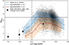 |
Fig. 2. Distribution of RPAH* vs. oxygen abundance for the entire sample of H II regions (gray histogram with intensity tracing the probability density), and average distribution for two bins in log([S III]/[S II]). The dashed lines are the same as in Fig. 1. The black squares represent measurements for WLM, NGC6822 (as in Fig. 1), the SMC, and the LMC from Chown et al. (2025a), listed in order of increasing metallicity. Spitzer IRAC4 and MIPS24 filters were used to estimate RPAH* for the SMC and LMC (Chown et al. 2025a). |
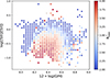 |
Fig. 3. RPAH* (see color bar at right) calculated on the regularly distributed bins with unique O/H and [S III]/[S II] values. The metallicity and ionization parameters are both important for setting up the PAH fraction. |
To check that the steep decrease in PAH fraction at low metallicities in our data is not just due to the different properties of the ionizing sources, we also measured RPAH* in diffuse ISM for different metallicity bins. To do that, we compiled a comparable sample of mock diffuse regions following a procedure similar to what Dale et al. (2025) performed for their analysis of star clusters and associations. We masked out all H II regions using the spatial masks (see Sec. 3.1), and then randomly selected the positions of circular apertures in the residual footprint. The diameter of the aperture was fixed at 3 × PSFMUSE for each galaxy to match the size of “resolved” H II regions (after rejecting the masked pixels). We discarded the regions where more than 50% pixels in the JWST MIRI/F2100W grid overlap with H II region masks. Repeating this procedure, we compiled a sample of the mock diffuse regions of comparable size and number per galaxy as for the H II regions. Then, we derived RPAH and RPAH* in the same way as for H II regions (Sec. 3.3). We assumed that these diffuse regions have a metallicity equal to the median for five nearest H II regions.
We divide all measurements for the diffuse and H II regions into several metallicity bins: 12 + log(O/H) = 7.9 − 8.2, 8.2 − 8.4, and 8.4 − 8.7. Fig. 4 shows distributions of RPAH* for each metallicity bin separately for the diffuse ISM and luminous (resolved) H II regions. Table 3 reports the median values of RPAH* and standard deviations for both types of regions per metallicity bin.
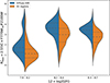 |
Fig. 4. Distribution of RPAH* for resolved (luminous) H II regions (orange) and the regions of similar size from the diffuse ISM (blue) for several gas-phase metallicity bins. The one dashed line and the two dotted lines on each distribution show the median and 25 and 75 percentile quartiles, respectively. Both RPAH and RPAH* are lower in the H II regions than in the diffuse ISM. A strong decrease in RPAH* in the lowest metallicity bin is seen for the H II regions and the diffuse ISM. |
Fig. 4 shows a significant decrease in RPAH* in H II regions compared to the diffuse ISM, consistent with a scenario where PAHs get destroyed in these nebulae. The two higher metallicity bins behave very similarly, reflecting the plateau in RPAH* at high metallicity. The lowest metallicity bin exhibits a significant decrease in RPAH* in both H II regions and the diffuse ISM. The differences between the lowest and moderate metallicity bins are in agreement with what was previously measured for the Magellanic Clouds (Chastenet et al. 2019). Therefore, the low-metallicity environment alters the PAH fraction in both environments in the same way.
4.2. Correlation between PAH fraction and ionization parameter at 50–100 pc scales
Observations of nearby galaxies with JWST revealed a fairly uniform distribution of RPAH in their diffuse ISM (Sutter et al. 2024). At the same time, the PAH fraction drops in H II regions or central regions with AGNs (Chastenet et al. 2023a; Egorov et al. 2023; Pedrini et al. 2024; Baron et al. 2024, 2025). This drop in H II regions at any metallicity (within the considered range) is clearly seen from the comparison of our sample of luminous H II regions with the diffuse ISM areas shown in Fig. 4. From the analysis of the vicinity of H II regions in four galaxies from the PHANGS sample, Egorov et al. (2023) discovered a strong anti-correlation between RPAH and log([SIII]/[SII]), which is a good tracer of the ionization parameter (see Appendix C). This dependence is also clearly seen in Fig. 3.
Figure 5 shows how RPAH changes with log([SIII]/[SII]) for a sample of 17151 H II regions (panel a). This figure shows that the dependence of PAH fraction on the ionization parameter found by Egorov et al. (2023) is observed across a ten-fold larger sample of H II regions than used in their work. Fig. 5c shows that the same trend is observed with expectedly smaller scatter if we keep only the luminous ∼5600 H II regions “resolved” by MUSE (i.e., having sizes exceeding 2 × FWHMPSF, according to our selection criteria described in Sec. 3.1). The best-fit linear regression model for the 2D distribution for the luminous H II regions gives the following relation:
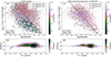 |
Fig. 5. PAH fraction anti-correlates with log([S III]/[S II]) (ionization parameter tracer) for thousands of H II regions in 42 PHANGS-JWST galaxies. Panels (a, b) shows all ∼17 200 analyzed H II regions, while the ∼5600 brightest resolved H II regions are shown in panels (c, d). The dashed red line shows the best-fit linear regression to the resolved sample defined by Eq. (4). The histograms in panels (b, d) show how the logarithmic residuals after subtracting this linear trend depend on metallicity. The color in panels (a, c) denotes gas-phase oxygen abundance; the red contours show the probability density of the high-metallicity (12 + log(O/H) > 8.2) points; the levels correspond to 50, 65, 80, 95, and 99 percentile intervals. The Spearman correlation coefficient (ρ) and RMS scatter around the linear fit are reported in panels (a, c). |
![Mathematical equation: $$ \begin{aligned} {R_{\rm PAH}^*} = (-4.37 \pm 0.52)\times \log (\mathrm{[SIII]/[SII]}) + (1.29\pm 0.16). \end{aligned} $$](/articles/aa/full_html/2025/11/aa56427-25/aa56427-25-eq12.gif) (4)
(4)
Coefficients and associated uncertainties are calculated using the orthogonal distance regression fitting to 500 bootstrapped samples. The same linear regression can also describe the unresolved regions in panel (a), although the scatter around it is higher, and the low-metallicity regions (12 + log(O/H) < 8.2) appear as outliers.
It is not clear what causes the scatter around the linear regression defined by Eq. (4). Egorov et al. (2023) tested several possible physical and observational parameters as potentially responsible for the observed scatter (including Q0 – the total number of ionizing photons, [O III]/Hβ as the UV hardness tracer, equivalent width of Hα as the age tracer, F1130W/F770W as a tracer of PAH ionization state), and found a secondary dependence of RPAH on metallicity (see their Fig. 3). Here we revisit this conclusion by reproducing the same analysis for a much larger sample of H II regions, especially in the lower metallicity range. We subtract the trend described by Eq. (4) from the data in Fig. 5 and demonstrate how the logarithmic residuals depend on the metallicity in panels b and d (for all and resolved only H II regions, respectively). The distribution of the residuals with metallicity is scattered around zero, but no obvious secondary dependence on metallicity is seen in the moderate- to high-metallicity regime in our data. The systematic deviation of the residuals from zero becomes prominent at low metallicities 12 + log(O/H) < 8.2.
Figure 5 demonstrates a purely observational result. Physically, the decrease in RPAH toward H II regions is consistent with scenarios of destruction or removal of PAH molecules. The fairly strong dependence of RPAH on the ionization parameter is indicative of the major role of the ionized gas in the evolution of PAH molecules in star-forming regions. Understanding the physical reasons (if any) behind such a relationship can provide clues about the mechanisms of PAH destruction. We consider in Sec. 5.2 several possible physical and observational effects that could be responsible for the observed dependence between the RPAH and the ionization parameter.
5. Discussion
5.1. Low- and high-metallicity regimes in the PAH life-cycle
Our observations clearly reveal dependence of the PAH fraction on metallicity (Figs. 1–4), which is consistent with previous resolved and unresolved studies of significantly smaller samples of star-forming regions (see Section 1). Several physical mechanisms can be responsible for the lower PAH fraction at low metallicities. Hard ionizing radiation at low metallicity could lead to more efficient destruction of PAHs, so they rarely survive in H II regions and inner layers of PDRs covered by our apertures. Alternatively, PAHs could form less efficiently (or have smaller sizes; Sandstrom et al. 2012; Whitcomb et al. 2024) in a low-metallicity environment. This is supported by significantly lower RPAH* (compared to high-metallicity bins, see Fig. 4) also in the diffuse ISM, where the processes of their photodestruction are less relevant. Another possible explanation is that PAHs can be destroyed by supernovae shocks more efficiently in low-metallicity environment because of the enhanced SNe rate in the low-mass star-forming galaxies (e.g., O’Halloran et al. 2006; Jackson et al. 2006; Seok et al. 2014). We address the role of shocks in selective PAH destruction in Section 5.3.
The highest metallicity regions in our sample (12 + log(O/H) > 8.55) also reveal a decrease in the PAH fraction (two last bins in Fig. 1), which cannot be explained by high [S III]/[S II] alone (Fig. 2). Such regions are located in the highest-mass galaxies from our sample. Although we excluded the galactic center regions from consideration, these high-metallicity regions are still associated with bars and other areas with much higher interstellar radiation field (from the old stellar population) than in spirals arms, which could result in decreased mid-IR emission, since the PAHs are being heated less effectively (Draine et al. 2014; Whitcomb et al. 2024; Baron et al. 2025; Pathak et al. in prep).
At intermediate metallicities, from 12 + log(O/H) ∼ 8.2 to ∼8.6, our observations find a constant average RPAH*, with values for particular regions highly correlated with the ionization parameter. This conclusion is consistent with the results obtained by Egorov et al. (2023), who found only a weak secondary dependence of RPAH on metallicity for H II regions from four PHANGS-JWST galaxies spanning a range of 12 + log(O/H) = 8.3 − 8.7 (its presence is not confirmed here with the larger sample), and Sutter et al. (2024), who found a remarkably constant RPAH across the diffuse ISM in the same metallicity range. The same behavior of PAH fraction with metallicity was reproduced by models of Hirashita & Murga (2020) considering PAH and dust destruction affecting the dust size distribution in the ISM. Meanwhile, Whitcomb et al. (2024) derived a higher threshold from the Spitzer-IRS spectral observations of the radial strips in three nearby galaxies: they found that the PAH fraction does not change significantly for 12 + log(O/H) > 8.5, below which it steeply drops. Although our results are in very good qualitative agreement with Whitcomb et al. (2024) findings, we try to understand why the quantitative measurements differ.
One of the explanations for such a discrepancy could be a systematic offset in the metallicity owing to the difference in the methodology. Whitcomb et al. (2024) estimated metallicity relying only on the oxygen abundance gradients and position of the region in the galaxy, while in our study we measure the oxygen abundances for each H II region individually (by using a strong emission line calibration). For the only overlapping galaxy in our samples – NGC 628 – there are differences in both central oxygen abundances and metallicity gradients assumed in their work (12 + log(O/H) = 8.69 − 0.09 × r/re measured by Rogers et al. 2021 using “direct” Te-method) and derived by Groves et al. (2023) using the same oxygen abundance measurements as in our work (12 + log(O/H) = 8.533 − 0.054 × r/re). Such differences, if they result in a systematic bias, can easily explain ∼0.1 dex of the overall discrepancy in the metallicity where PAH fraction drops sharply. The discrepancies between empirical strong-line and “direct” methods are not surprising and are a long-standing problem (see, e.g., Kewley & Ellison 2008). However, Scal and Te calibration typically show reasonable agreement (e.g., Brazzini et al. 2024), and therefore differences in the methods alone are unlikely to explain ∼0.3 dex systematic shift in the metallicity of the threshold.
Our photometric approach to calculating the PAH fraction utilizes information about only a small number of PAH features, and does not allow precise continuum estimates, and thus can have some bias compared to spectral measurements. Whitcomb et al. (2024) is based on spectral observations, and compares all PAH emission to the total IR brightness (ΣPAH/TIR). As this correlates linearly with the PAH mass fraction, their ΣPAH/TIR can be scaled to RPAH*, to allow a more direct comparison. Estimating the average ΣPAH/TIR and RPAH* for the NGC 628 regions in both datasets, we find RPAH* ≃ 0.22 × ΣPAH/TIR. Using this scaling factor, we converted the results from Whitcomb et al. (2024) (using the average values in bins in their Fig. 4) to RPAH*, and show them as an orange line overlaid on our measurements in Fig. 6.
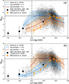 |
Fig. 6. Same as Fig. 2, but here the blue and red curves correspond to different bins of low and high [O III]/Hβ (panel a) or [S II]/Hα (panel b), respectively. The orange curve and points are translated from the average values per metallicity bin in Fig. 4 in Whitcomb et al. (2024). |
This comparison indicates another possible origin for the discrepancy in the threshold between the high- and low-metallicity regimes. Splitting our data into two subsamples with high and low [O III]/Hβ or [S II]/Hα (similarly to Fig. 2 for [S III]/[S II]), we find that considering only hard and soft ionization regions (that is, with high [O III]/Hβ and low [S II]/Hα, and vice versa) can lead to systematic differences in the position of the metallicity threshold: harder ionization regions exhibit a higher metallicity turnover. Interestingly, the low-metallicity end of the Whitcomb et al. (2024) curve coincides very well with our measurements when only regions with relatively hard ionizing spectra are considered. However, since their data in this tail correspond to kpc-sized bins that include diffuse ISM and H II regions, such ionization bias is very unlikely, and systematics in metallicity estimates remain the most probable explanation.
5.2. Is the PAH fraction physically linked with the properties of ionized gas?
By construction, each point in Fig. 5 represents an H II region. High physical resolution observations of a small subset of Galactic nebulae reveal sharp borders in the PAH emission (e.g., Hernández-Vera et al. 2023; Abergel et al. 2024; Chown et al. 2024). Given this, one can expect that efficient PAH destruction would produce much lower values of RPAH* than what is observed in Fig. 5. The PAH fraction should be around zero in all (especially the brightest) H II regions, which approximately corresponds to RPAH* ∼ 0.5 (see Fig. 7 in Sutter et al. 2024). However, such sharp borders between PAH emission and H II regions cannot be observed in relatively distant extragalactic objects even if the ionized gas is traced by high-resolution Paα JWST images (Pedrini et al. 2024). Instead, we see a gradual decrease with the ionization parameter even for the brightest “resolved” H II regions (Fig. 5c), with non-zero PAH fraction at any measured ratio of [S III]/[S II] (with the exception of some of the lowest metallicity regions). Here we consider physical and observational effects that can be responsible for the measured non-zero PAH fractions in H II regions and setting such a uniform observational trend with the [S III]/[S II] present across all galaxies in our sample. For all tests in the rest of this Section, we rely on RPAH (not RPAH*) measurements, which include the 7.7 μm and 11.3 μm PAH bands and are not dependent on the luminosity-sensitive conversion between RPAH* and RPAH. However, the results remain unchanged when using RPAH*.
5.2.1. Physical connection between the PAH fraction and the number of EUV photons.
By definition, the ionization parameter is proportional to the number of hydrogen-ionizing photons relative to the number of hydrogen atoms. The more such extreme UV (EUV) photons are present in a region, the higher the ionization parameter, and the more PAH molecules are exposed by such harsh ionizing radiation. Laboratory studies find that large PAHs are mostly photoionized when exposed to energies above 13.6 eV, and start experiencing photodissociation at energies below 20 eV (Wenzel et al. 2020). Because most EUV photons have the potential to destroy PAHs, it is primarily the number density of EUV photons and not the hardness of the UV spectrum that determines the efficiency of PAH destruction. The latter explains the absence of the secondary dependence of RPAH on [O III]/Hβ and metallicity for the high metallicity range (Figs. 5, 6, see also Egorov et al. 2023). From modeling, Murga et al. (2019) found that the characteristic timescale for the photodestruction of PAH-like grains decreases significantly with increasing radiation field intensity, providing another physical basis for the observed anti-correlation between RPAH and the ionization parameter. Overall, the scenario of ionization of PAHs and their subsequent destruction (through photodestruction or sputtering and fragmentation) regulated by the intensity of EUV ionizing radiation (and hence – ionization parameter) is consistent with the observed decrease in the RPAH in the H II regions compared to diffuse ISM (Fig. 4, see also Sutter et al. 2024; Pedrini et al. 2024).
5.2.2. PDRs dominate theRPAHmeasurements due to limited resolution.
As described in Sec. 3.1, we identified the borders of the H II regions based on the MUSE data, which have angular (and spatial) resolution lower than that of the JWST images. At the distance of our sample, our spatial masks defining borders of H II regions are not perfectly isolating them from the PDRs where the emission of PAHs dominates (e.g., Anderson et al. 2014). Even if the small number of H II regions in our sample are truly resolved, we still expect to see a contribution from PDRs and the diffuse ISM along the line-of-sight. Therefore, the non-zero values of RPAH can be naturally explained if the RPAH values reflect a combination of the surrounding diffuse ISM, PDRs, and the H II region within the nebular mask boundary. The observed anti-correlation could also reflect the strong link between the properties of the surrounding ISM (including PDRs) and ionized gas in H II regions. In particular, due to the leaky nature of H II regions (e.g., Oey et al. 2007; Della Bruna et al. 2021; Ramambason et al. 2020; Teh et al. 2023), EUV radiation can penetrate into surrounding ISM and ionize or destroy PAHs there, as described above. Therefore, the results in Fig. 5 can reflect the processes occurring in the zones of influence of H II regions rather than in H II regions themselves.
To test whether our measurements of RPAH are indeed significantly affected by the overestimated sizes of H II spatial masks, we compare the values of RPAH measured in circular apertures with radii equal to rcirc, 0.5 × rcirc, 0.25 × rcirc, where rcirc is circularized radius of the H II region derived from MUSE data, to the value recovered at the location of a local peak in Hα distribution within the H II region mask. The results of our test are shown in Fig. 7, where different colors correspond to distribution of the RPAH measured in the chosen aperture relative to that at the location of Hα peak, where  is supposed to be minimal.
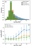 |
Fig. 7. About 45% of the RPAH measurements are overestimated by more than 10% when measured in the MUSE-based apertures for H II regions compared to the values in their centers. Panel (a) shows the probability distribution of RPAH measured in different circular apertures for the same sample of H II regions related to the value of RPAH measured at the local peaks of Hα brightness within the H II region. Panel b demonstrate how such ratios change for different Hα luminosity bins. The different colors correspond to different outer radii of the circular aperture. |
We do not see significant differences between the measurements made in the two reduced apertures compared to  and to each other. However, about 45% of regions show higher RPAH by at least 10% when measured in the largest aperture corresponding to the adopted size of the H II regions in our analysis. As follows from Fig. 7b, the difference is greater in brighter regions, which likely indicates that we cannot isolate diffuse ISM from H II regions at all in the faintest areas using the JWST MIRI/F2100W resolution in our sample.
From this test, we can conclude that our integrated measurements in Fig. 5 are contaminated by a contribution from the PDR and surrounding diffuse ISM due to insufficient resolution to isolate H II regions. To test if this fact alone is responsible for the observed anti-correlation between RPAH and the ionization parameter, we tested also how RPAH* measured at the Hα peaks of the “resolved” H II regions changes with [S III]/[S II] and did not find significant differences with the Fig. 5c – the anti-correlation remains strong and can be fitted by Eq. (4). Therefore, we can rule out that this relation is the consequence of the aperture effect alone.
We note that the same effect as seen in Fig. 7 could be in principle observed even if our data allowed the perfect isolation of H II regions provided that PAHs are not completely destroyed or removed at the edges of H II regions. Recent JWST observations of the Horsehead nebula (Abergel et al. 2024) revealed photoevaporative flows from PDRs to the interior of the H II region visible in F770W and F335M filters centered on PAHs. The characteristic length of such features (∼0.05 pc) is much smaller than can be resolved in similar extragalactic regions. However, as was demonstrated by recent SDSS-V/LVM IFU observations, the central region of Orion (which includes the Horsehead nebula) is not representative of the population of extragalactic H II regions (Kreckel et al. 2024). Therefore, in principle, such an effect could be more prominent in the regions surrounding more energetic sources like what is seen in the PHANGS sample of H II regions. Furthermore, Bolatto et al. (2024) observed PAH emission closely resembling the ionized gas in outflow of M82 and argued that part of it can come from the surviving PAHs at the interface between the ionized and neutral ISM. Future statistical morphological analysis of a large sample of regions in the Local Group galaxies with very high resolution for both ionized gas (e.g., with the Paα emission line) and PAHs (using 3.35 μm feature) with JWST can provide clues about how steep the decrease in PAH abundance is in normal H II regions.
5.2.3. Time evolution of PAHs.
Independently of whether the result presented in Fig. 5 reflects the processes in H II regions or in the PDRs, the general behavior of this plot can be attributed also to the time evolution of the H II regions. Theoretical models and observational works demonstrate that at fixed H II region luminosity, the ionization parameter decreases as a function of time (e.g., Dopita et al. 2006; Scheuermann et al. 2023). From photoionization models, it follows that the observed line ratio [S III]/[S II] also decreases with the age of the ionizing star cluster even at the fixed value of ionization parameter (see Fig. C.1 in Appendix C). Therefore, the anti-correlation between RPAH and the [S III]/[S II] observed in Fig. 5 could reflect a time evolution of the PAH fraction in the ISM illuminated by EUV radiation, where each bin along the x-axis could be interpreted as a time stamp. However, a lack of correlation between RPAH and EW(Hα), another good tracer of the age of H II regions, makes this interpretation unlikely (Egorov et al. 2023).
5.2.4. Line-of-sight projection of the diffuse ISM onto H II regions.
Star-forming regions are embedded in the large reservoirs of the diffuse ISM. Therefore, some contamination of the measured fluxes in optical emission lines (from DIG) and in mid-IR bands (from neutral diffuse ISM) is expected. The absolute brightness of [S II] and especially [S III] is typically much lower in DIG than in H II regions, and thus its contribution along the line of sight should not significantly affect the observed [S III]/[S II] and the ionization parameter for most of the regions. Egorov et al. (2023) demonstrated that the anti-correlation between RPAH and the ionization parameter remains unchanged when only H II regions with high contrast over DIG are considered. The contamination of RPAH measurements by line of sight emission from the neutral ISM can be however much higher as the fluxes in mid-IR bands are typically high outside the star-forming regions (Leroy et al. 2023; Sandstrom et al. 2023b; Pathak et al. 2024). Below we consider if such contamination alone can explain the observed relation in Fig. 5.
To test this, we consider here a toy model of a spherical H II region with radius rHII located at the mid-plane of the galactic disk. We assume that the vertical density distribution of the dust in the disk is mimicking the gas density distribution and can be described by a Gaussian with the disk scale height hd. Also, we assume that the H II region is completely devoid of PAHs, and outside the H II region their volumetric density is distributed according to the same law as for dust grains. The latter assumption is in agreement with the findings by Sutter et al. (2024), who measured fairly constant distribution of RPAH ∼ 3.43 across the diffuse ISM of 19 PHANGS galaxies. We therefore assume in our toy model that outside the H II region, RPAH = RPAH0 = 3.43. Then we can estimate how RPAH should change with the size of H II region assuming that all PAHs that we observe toward H II region are from the diffuse ISM along the line of sight:
 (5)
(5)
where MPAH and Mdust are total masses of the PAHs and small grains along the line-of-sight in the aperture limited by the H II region footprint, ρPAH, ρdust, ρPAH0 and ρdust0 are volumetric densities of the PAHs and small dust grains in the particular volume dV and in the midplane of galactic disk outside H II region, respectively; z is the distance along the line-of-sight from the midplane; i is inclination of the galactic disk; SHII and VHII are the area in the galactic plane and the volume occupied by the H II region, respectively. We note as one of the caveats that this toy model does not account for the probable increase in PAH and dust masses and luminosities around the H II regions.
By definition, the ionization parameter is proportional to  , which means that it decreases with the expansion of the H II region (assuming constant density and ionizing flux). Photoionization models also reveal such a trend for [S III]/[S II] line ratio: while [S III]/[S II] increases with the ionizing photons rate Q0, it decreases with the radius of the region for each constant value of Q0 (see Appendix C). Therefore, to some extent, the [S III]/[S II] ratio should correlate with the size of the regions, and thus it can be assumed that the observed trend between RPAH and [S III]/[S II] can result from the RPAH vs. rHII relation, which in turn is expected from our toy model according to Eq. (5).
In Fig. 8a, we check if RPAH correlates with the H II size and if this correlation can be explained by our toy model. As a proxy of rHII, we consider circularized radii of H II regions  derived by Barnes et al. (2025) from HST Hα narrow-band images (Chandar et al. 2025) for about 5000 H II regions in 19 PHANGS-JWST Cycle 1 galaxies. Unlike MUSE Hα images, HST observations resolve H II regions and provide more reliable measurements of their sizes. We indeed see the anti-correlation between sizes and RPAH. However, the scatter is much higher and the significance of the correlation is much weaker than for the RPAH vs [S III]/[S II] shown in panel b for the same subsample of regions and in the same 2D histogram representation for comparison. Note that the sizes in panel a are multiplied by cos(i) to take into account the galaxy inclination in the same way as in Eq. (5) for further comparison with the toy model. However, the scatter and the correlation coefficient improve insignificantly for the uncorrected values.
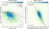 |
Fig. 8. Histograms showing distribution of RPAH vs. the logarithm of the circularized radii of the H II regions derived from HST data (from Barnes et al. 2025; panel (a)), and vs the ionization parameter tracer log([SIII]/[SII]) (panel (b)). The colors denote the number of regions in each bin. The curved dashed, solid, and dotted lines in panel (a) show models defined by Eq. (5) with the disk scale height hd = 50, 100, and 400 pc, respectively. The red dashed line in panel (b) corresponds to Eq. (4). The anti-correlation between RPAH and the size of the H II region is much weaker than that with the ionization parameter, and can be partially explained by the contribution of the PAHs from the diffuse ISM along the line of sight. |
In Fig. 8a, we overlaid the distribution of RPAH according to Eq. (5) for three adopted values of the PAH scale height: hd = 50, 100 and 400 pc. Our toy model generally shows reasonable agreement with the observations assuming hd = 50 pc, which is measured for molecular gas (Jeffreson et al. 2022), or hd = 100 pc, which is a fiducial scale height for the star-forming disks (Schinnerer & Leroy 2024) in spiral galaxies. However, a single value of hd cannot reproduce the whole range of RPAH measurements, and our toy model overestimates RPAH for the largest regions. The latter can be in principle explained by the violation of the assumption of spherical symmetry for the large H II regions that have a size comparable to the disk scale height. The model significantly overestimates RPAH if the PAHs are assumed to be distributed in a disk with hd ∼ 200 − 400 pc, which is typically estimated for H I in the central parts of galaxies (e.g., Yim et al. 2014; Bacchini et al. 2019; Patra 2020). Overall, observations show a steeper decrease in RPAH with growing  than is seen in the model. Furthermore, if
  still overestimates the sizes of the H II regions, the observational data would shift further to the left of the model lines. Barnes et al. (2025) showed that the sizes indeed appear to be smaller than
  by ∼0.3 dex when computed from the second spatial moments of the emission within the source boundary. Therefore, we can conclude that within the assumption in our toy model, the effect of the line-of-sight projection can only partially explain RPAH vs
  (and to some extent – vs. [S III]/[S II]) if PAHs are distributed in the thin star-forming disk with scale height comparable to what is typically measured for molecular gas. Note, however, that the observations show that PAHs are also mixed with atomic gas in our Galaxy (e.g., Boulanger et al. 1985; Puget et al. 1985; Dwek et al. 1997), which means that they are not necessarily locked in such a thin disk.
To summarize this section, we conclude that most of the mechanisms considered here can contribute to the observed relation between RPAH and the ionization parameter. Contamination by diffuse ISM along the line of sight can lead to a higher RPAH at lower [S III]/[S II] ratio due to the secondary dependence of this ratio on the size of the H II region, although such projection effect alone is unlikely to completely explain the observed tight anti-correlation. The limited spatial resolution does not allow us to perfectly isolate the interiors of the H II regions from the PDRs, and therefore this relation probably reflects a link between the processes in the PDRs and the properties of the ionized gas. These processes lead to a decrease in RPAH in regions with a high ionization parameter (i.e., a high density of ionizing photons), while the hardness of the ionizing radiation is not important in the moderate- to high-metallicity regime. Regardless of whether these processes occur in PDRs or in the interface between ionized and neutral gases in the H II regions, the overall picture is consistent with the scenario in which PAHs are ionized and destroyed by hydrogen-ionizing photons. In the meantime, the particular physical mechanisms regulating PAH destruction remain uncertain, and the analysis of other spectral features sensitive to the physical properties of PAHs is thus required. In particular, upcoming 3.3 μm maps for PHANGS galaxies (Koizol et al., in prep.; Sandstrom et al. 2023b), combined with the 7.7 μm and 11.3 μm data presented here, will provide diagnostics of whether PAHs are destroyed primarily by ionization or by changes in their sizes (e.g., Draine et al. 2021; Baron et al. 2024; Dale et al. 2025).
5.3. PAH fraction is insensitive to SNe shocks at 50 pc scale
In previous sections, we focused mainly on the observational signatures of PAH destruction in the H II regions caused by the influence of EUV radiation. Meanwhile, theoretical works and observations suggest that shocks could also destroy PAHs (e.g., O’Halloran et al. 2006; Micelotta et al. 2010b; Zhang et al. 2022). In particular, more efficient PAH destruction by SNe shocks in low-metallicity galaxies was considered as one possible explanation of the metallicity dependence of the PAH fraction. PHANGS galaxies provide an excellent opportunity to test the role of supernova shocks in selective PAH destruction. In a recent paper, Li et al. (2024) presented a catalog of 964 isolated SNRs carefully selected with five different criteria (see details in Section 3.1). Here we analyze how RPAH averaged in 50 pc circular apertures around these isolated SNRs differs from what is derived in H II regions and the diffuse ISM and search for indications of the more localized signatures of PAH selective destruction.
Figure 9a shows the similar correlation between RPAH and the ionization parameter as in Fig. 5b with overlaid measurements for SNRs. As seen from this plot, SNRs typically have a smaller range of [S III]/[S II], which is expected as they have different ionization mechanisms compared to H II regions. Most SNRs are concentrated in the upper left part of the RPAH vs. [S III]/[S II] relation defined by Eq. (4), although RPAH for SNRs does not seem to depend strongly on [S III]/[S II] in the same way as it does for H II regions. However, assuming that Eq. (4) reflects the effects of photoionization and photodestruction of PAHs, not seeing such a clear dependence for SNRs is not surprising.
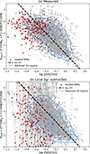 |
Fig. 9. Distribution of RPAH vs. log([SIII]/[SII]) for the resolved H II regions (gray points; as in Fig. 5c) and isolated SNRs (red points). Panels (a) and (b) correspond to RPAH measurements from the observed and the local background subtracted fluxes. The black dashed line corresponds to the relation defined by Eq. (4). The cyan contours show the probability density distribution for H II regions; the levels correspond to 65, 80, 95, and 99 percentile intervals. |
In Fig. 10a, we compare RPAH for SNRs and diffuse ISM for the two metallicity bins covered by the Li et al. (2024) sample in the same way as we did for H II regions in Sec. 4.1. If shocks are important for selective PAH destruction, and if their effect can be measured at 50 pc scales, we would expect to see lower RPAH for SNRs compared to diffuse ISM. However, we do not see any significant differences in Fig. 9a or 10a.
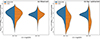 |
Fig. 10. Same as Fig. 4, but for SNRs (orange) compared to the diffuse ISM (blue). Panels (a) and (b) correspond to RPAH measurements from the observed and the local background subtracted fluxes. SNRs do not reveal a decrease in RPAH measured from the observed fluxes indicating that SN shocks are unlikely major contributors to the selective PAH destruction at 50 pc scale. A more localized effect is evident from the background-subtracted measurements. |
The SNRs are often faint in mid-IR emission and show limited contrast with the background. To better isolate the localized effects of SNRs, we repeat the same analysis by measuring RPAH from the local background-subtracted fluxes, as described in Sec. 3.3. About 65% of the original sample of SNRs reveal the signal in all three considered MIRI bands after the backround removal, thus ensuring that the measured residual signal from SNRs is not a result of random fluctuations. For comparison, similar background subtraction for diffuse ISM regions (which are nearly homogeneous by construction) resulted in 34% positive residuals, which is close to what is expected from the noise distribution. The resulting values of RPAH are scattered on the RPAH vs. [S III]/[S II] plot (Fig. 9b) demonstrating that the correlation defined by Eq. (4) is not applicable for SNRs. Meanwhile, we can recover the lower RPAH at the SNRs locations compared to the original measurements for diffuse ISM in Fig. 10b.
This test demonstrates that the effects of SNe shocks on the PAH fraction without a diffuse background correction are indistinguishable in unresolved studies, most likely because of the dominant contribution of the IR emission from the diffuse ISM in the aperture. Therefore, the signatures of the selective PAH destruction by shocks can be identified at the SNR locations, but is not dominant on 50 pc scales as high contamination by the diffuse ISM prevents their detection. This means that selective PAH destruction by SN shocks, suggested earlier to explain the decrease in the PAH fraction at low metallicities, is unlikely to affect a global PAH fraction on galaxy scales.
6. Summary
Based on the JWST MIRI and NIRCam imaging and MUSE integral field spectroscopic observations of 42 nearby galaxies, we investigated how the dust mass fraction of PAHs traced by mid-IR emission (RPAH) is linked to and/or regulated by the properties of the ionized gas in star-forming regions. The galaxies in our sample are from the PHANGS sample and cover stellar masses from 1.5 × 10⁹ to 1.2 × 10¹¹ M⊙, with individual H II regions having oxygen abundances mostly from 12 + log(O/H) from 8.0 to 8.8 (i.e., 0.2 − 1.3 Z⊙) and located at distances from 5 to 23 Mpc (i.e., allowing spatial resolution of < 100 pc with MUSE and < 80 pc with JWST at 21 μm, the longest wavelength considered here). Using the spatial masks (derived from the MUSE Hα images), we isolated the H II regions from the diffuse ISM and measured the RPAH ratio, which traces PAH fraction, for every H II region and a control sample of diffuse ISM regions. For 19 more massive (and metal-rich) galaxies, we also measured RPAH in the circular 50 pc apertures surrounding the sample of SNRs isolated from H II regions. Comparing the measured values of RPAH with the properties of the ionized gas, we obtained the following main results:
-
The PAH fraction drops at metallicities 12 + log(O/H) < 8.2 in H II regions and in the diffuse ISM. Above this limit, it is relatively insensitive to metallicity. PAHs could be destroyed more efficiently in the low-metallicity H II regions due to the higher UV hardness. At the same time, the same steep decrease for the diffuse ISM indicates a possible less efficient formation of PAHs in low-metallicity environments.
-
The PAH fraction for H II regions is significantly lower than for the diffuse ISM at all metallicities considered here. We argue that PAHs are being destroyed in H II regions by intense hydrogen-ionizing radiation.
-
We find a strong anticorrelation between RPAH and the ionization parameter (traced by the log([SIII]9069/[SII]6717 + 6731) emission line ratio) across our large sample of relatively high-metallicity H II regions with 12 + log(O/H) > 8.2.
-
We argue that the relation between the PAH fraction and the ionization parameter is driven by a physical connection between the properties of the ionized gas and PAHs at the edges of H II regions and PDRs. Assuming that PAHs are distributed in the thin disk, the effects of line-of-sight projection also contribute significantly to the observed relation, but cannot completely explain it.
-
We do not see differences in the PAH fraction between diffuse ISM and isolated SNRs when measured from the observed JWST/MIRI band ratios. Only by applying careful local background subtraction do we recover evidence of PAH destruction at SNR sites. This indicates that supernova shocks do not contribute significantly to the selective PAH destruction when averaged over 50 pc scales. In particular, the previously suggested explanation of the metallicity dependence of the PAH fraction resulting from higher SN activity in low-metallicity galaxies seems to be unlikely.
Overall, our results agree with the scenario of PAH ionization and destruction by hydrogen-ionizing photons in star-forming regions, and of less efficient formation of PAHs in the low-metallicity environment. The particular physical mechanisms, spatial scales and timescales for PAH destruction remain unclear. Future systematic resolved studies of extragalactic H II regions and their surroundings now possible with JWST by imaging of the ionized gas (via Paα emission line) and the small PAHs glowing at 3.3 μm, or by resolved spectroscopy with NIRSpec and MIRI-MRS will certainly provide a huge next step in our understanding of the PAH evolution cycle.
Data availability
The catalog with our measurements described in Appendix D is available at the CDS via https://cdsarc.cds.unistra.fr/viz-bin/cat/J/A+A/703/A103
This size roughly corresponds to the resolution of the JWST MIRI F2100W images for the most distant galaxies in our sample; using diameters of 100 pc, as in Li et al. 2024 paper, or 25 pc does not affect the results presented below.
Acknowledgments
This work is based on observations made with the NASA/ESA/CSA JWST. The data were obtained from the Mikulski Archive for Space Telescopes at the Space Telescope Science Institute, which is operated by the Association of Universities for Research in Astronomy, Inc., under NASA contract NAS5-03127. The observations are associated with JWST programs 2107 and 3707. The specific observations analyzed can be accessed via https://doi.org/10.17909/ew88-jt15. Based on observations collected at the European Southern Observatory under ESO programmes 0111.C-2109 (PI: Egorov), 0108.B-0249 (PI: Kreckel), 094.C-0623 (PI: Kreckel), 095.C-0473, 098.C-0484 (PI: Blanc), 1100.B-0651 (PHANGS-MUSE; PI: Schinnerer), as well as 094.B-0321 (MAGNUM; PI: Marconi), 096.B-0309, 098.B-0551, 099.B-0242, 0100.B-0116 (MAD; PI: Carollo), 097.B-0640 (TIMER; PI: Gadotti), 0104.B-0404, 109.22VU.001 (PI: Erwin), 094.B-0298 (PI: Walcher), 60.A-9487 (PI: Gadotti), 109.2332.001 (PI: Belfiore), 0102.B-0617 (PI: Fluetsch), 111.24KE.001 (PI: Barnes), 097.D-0408 (PI: Anderson). OE acknowledges funding from the Deutsche Forschungsgemeinschaft (DFG, German Research Foundation) – project-ID 541068876. MB gratefully acknowledges support from the ANID BASAL project FB210003. This work was supported by the French government through the France 2030 investment plan managed by the National Research Agency (ANR), as part of the Initiative of Excellence of Université Côte d’Azur under reference number ANR-15-IDEX-01. KK, MCS, EE, MH, and JL acknowledge support from the Deutsche Forschungsgemeinschaft (DFG, German Research Foundation) in the form of an Emmy Noether Research Group (grant number KR4598/2-1, PI Kreckel) and the European Research Council’s starting grant ERC StG-101077573 (“ISM-METALS”). HK, KS acknowledge funding from JWST-GO-2107.006-A. HAP acknowledges support from the National Science and Technology Council of Taiwan under grant 113-2112-M-032-014-MY3. JC acknowledges funding from the Belgian Science Policy Office (BELSPO) through the PRODEX project “JWST/MIRI Science exploitation” (C4000142239).
References
- Abergel, A., Misselt, K., Gordon, K. D., et al. 2024, A&A, 687, A4 [NASA ADS] [CrossRef] [EDP Sciences] [Google Scholar]
- Allain, T., Leach, S., & Sedlmayr, E. 1996, A&A, 305, 602 [NASA ADS] [Google Scholar]
- Anand, G. S., Lee, J. C., Van Dyk, S. D., et al. 2021a, MNRAS, 501, 3621 [Google Scholar]
- Anand, G. S., Rizzi, L., Tully, R. B., et al. 2021b, AJ, 162, 80 [CrossRef] [Google Scholar]
- Anderson, L. D., Bania, T. M., Balser, D. S., et al. 2014, ApJS, 212, 1 [Google Scholar]
- Aniano, G., Draine, B. T., Gordon, K. D., & Sandstrom, K. 2011, PASP, 123, 1218 [Google Scholar]
- Aniano, G., Draine, B. T., Hunt, L. K., et al. 2020, ApJ, 889, 150 [NASA ADS] [CrossRef] [Google Scholar]
- Asplund, M., Grevesse, N., Sauval, A. J., & Scott, P. 2009, ARA&A, 47, 481 [NASA ADS] [CrossRef] [Google Scholar]
- Bacchini, C., Fraternali, F., Iorio, G., & Pezzulli, G. 2019, A&A, 622, A64 [NASA ADS] [CrossRef] [EDP Sciences] [Google Scholar]
- Baldwin, J. A., Phillips, M. M., & Terlevich, R. 1981, PASP, 93, 5 [Google Scholar]
- Barnes, A. T., Chandar, R., Kreckel, K., et al. 2022, A&A, 662, L6 [NASA ADS] [CrossRef] [EDP Sciences] [Google Scholar]
- Barnes, A. T., Chandar, R., & Kreckel, K. 2025, A&A, in press, https://doi.org/10.1051/0004-6361/202555751 [Google Scholar]
- Baron, D., Sandstrom, K. M., Rosolowsky, E., et al. 2024, ApJ, 968, 24 [NASA ADS] [CrossRef] [Google Scholar]
- Baron, D., Sandstrom, K. M., Sutter, J., et al. 2025, ApJ, 978, 135 [Google Scholar]
- Belfiore, F., Santoro, F., Groves, B., et al. 2022, A&A, 659, A26 [NASA ADS] [CrossRef] [EDP Sciences] [Google Scholar]
- Belfiore, F., Leroy, A. K., Williams, T. G., et al. 2023, A&A, 678, A129 [NASA ADS] [CrossRef] [EDP Sciences] [Google Scholar]
- Binder, B. A., & Povich, M. S. 2018, ApJ, 864, 136 [CrossRef] [Google Scholar]
- Bittner, A., Falcón-Barroso, J., Nedelchev, B., et al. 2019, A&A, 628, A117 [NASA ADS] [CrossRef] [EDP Sciences] [Google Scholar]
- Bocchio, M., Micelotta, E. R., Gautier, A. L., & Jones, A. P. 2012, A&A, 545, A124 [NASA ADS] [CrossRef] [EDP Sciences] [Google Scholar]
- Bolatto, A. D., Simon, J. D., Stanimirović, S., et al. 2007, ApJ, 655, 212 [NASA ADS] [CrossRef] [Google Scholar]
- Bolatto, A. D., Levy, R. C., Tarantino, E., et al. 2024, ApJ, 967, 63 [NASA ADS] [CrossRef] [Google Scholar]
- Boulanger, F., Baud, B., & van Albada, G. D. 1985, A&A, 144, L9 [Google Scholar]
- Brazzini, M., Belfiore, F., Ginolfi, M., et al. 2024, A&A, 691, A173 [NASA ADS] [CrossRef] [EDP Sciences] [Google Scholar]
- Burkhardt, A. M., Long Kelvin Lee, K., Bryan Changala, P., et al. 2021, ApJ, 913, L18 [NASA ADS] [CrossRef] [Google Scholar]
- Bushouse, H., Eisenhamer, J., Dencheva, N., et al. 2023, JWST Calibration Pipeline [Google Scholar]
- Calapa, M. D., Calzetti, D., Draine, B. T., et al. 2014, ApJ, 784, 130 [NASA ADS] [CrossRef] [Google Scholar]
- Calzetti, D., Kennicutt, R. C., Engelbracht, C. W., et al. 2007, ApJ, 666, 870 [Google Scholar]
- Chandar, R., Barnes, A. T., Thilker, D. A., et al. 2025, AJ, 169, 150 [Google Scholar]
- Chastenet, J., Bot, C., Gordon, K. D., et al. 2017, A&A, 601, A55 [NASA ADS] [CrossRef] [EDP Sciences] [Google Scholar]
- Chastenet, J., Sandstrom, K., Chiang, I.-D., et al. 2019, ApJ, 876, 62 [NASA ADS] [CrossRef] [Google Scholar]
- Chastenet, J., Sutter, J., Sandstrom, K., et al. 2023a, ApJ, 944, L11 [NASA ADS] [CrossRef] [Google Scholar]
- Chastenet, J., Sutter, J., Sandstrom, K., et al. 2023b, ApJ, 944, L12 [NASA ADS] [CrossRef] [Google Scholar]
- Chastenet, J., Sandstrom, K., Leroy, A. K., et al. 2025, ApJS, 276, 2 [Google Scholar]
- Cherchneff, I., Barker, J. R., & Tielens, A. G. G. M. 1992, ApJ, 401, 269 [Google Scholar]
- Chown, R., Sidhu, A., Peeters, E., et al. 2024, A&A, 685, A75 [NASA ADS] [CrossRef] [EDP Sciences] [Google Scholar]
- Chown, R., Leroy, A. K., Bolatto, A. D., et al. 2025a, ApJ, 987, 91 [Google Scholar]
- Chown, R., Leroy, A. K., Sandstrom, K., et al. 2025b, ApJ, 983, 64 [Google Scholar]
- Cluver, M. E., Jarrett, T. H., Dale, D. A., et al. 2017, ApJ, 850, 68 [Google Scholar]
- Congiu, E., Blanc, G. A., Belfiore, F., et al. 2023, A&A, 672, A148 [NASA ADS] [CrossRef] [EDP Sciences] [Google Scholar]
- Dale, D. A., Boquien, M., Barnes, A. T., et al. 2023, ApJ, 944, L23 [NASA ADS] [CrossRef] [Google Scholar]
- Dale, D. A., Graham, G. B., Barnes, A. T., et al. 2025, AJ, 169, 133 [Google Scholar]
- Della Bruna, L., Adamo, A., Lee, J. C., et al. 2021, A&A, 650, A103 [NASA ADS] [CrossRef] [EDP Sciences] [Google Scholar]
- Diaz, A. I., Terlevich, E., Vilchez, J. M., Pagel, B. E. J., & Edmunds, M. G. 1991, MNRAS, 253, 245 [NASA ADS] [CrossRef] [Google Scholar]
- Dopita, M. A., Fischera, J., Sutherland, R. S., et al. 2006, ApJ, 647, 244 [NASA ADS] [CrossRef] [Google Scholar]
- Draine, B. T., & Li, A. 2007, ApJ, 657, 810 [CrossRef] [Google Scholar]
- Draine, B. T., Dale, D. A., Bendo, G., et al. 2007, ApJ, 663, 866 [NASA ADS] [CrossRef] [Google Scholar]
- Draine, B. T., Aniano, G., Krause, O., et al. 2014, ApJ, 780, 172 [Google Scholar]
- Draine, B. T., Li, A., Hensley, B. S., et al. 2021, ApJ, 917, 3 [CrossRef] [Google Scholar]
- Dwek, E., Arendt, R. G., Fixsen, D. J., et al. 1997, ApJ, 475, 565 [NASA ADS] [CrossRef] [Google Scholar]
- Egorov, O. V., Kreckel, K., Sandstrom, K. M., et al. 2023, ApJ, 944, L16 [NASA ADS] [CrossRef] [Google Scholar]
- Emsellem, E., Schinnerer, E., Santoro, F., et al. 2022, A&A, 659, A191 [NASA ADS] [CrossRef] [EDP Sciences] [Google Scholar]
- Engelbracht, C. W., Gordon, K. D., Rieke, G. H., et al. 2005, ApJ, 628, L29 [NASA ADS] [CrossRef] [Google Scholar]
- Engelbracht, C. W., Rieke, G. H., Gordon, K. D., et al. 2008, ApJ, 678, 804 [NASA ADS] [CrossRef] [Google Scholar]
- Ferland, G. J., Chatzikos, M., Guzmán, F., et al. 2017, Rev. Mex. Astron. Astrofis., 53, 385 [NASA ADS] [Google Scholar]
- Galliano, F., Dwek, E., & Chanial, P. 2008, ApJ, 672, 214 [NASA ADS] [CrossRef] [Google Scholar]
- Gao, Y., Xiao, T., Li, C., et al. 2019, ApJ, 887, 172 [Google Scholar]
- Gao, Y., Tan, Q.-H., Gao, Y., et al. 2022, ApJ, 940, 133 [NASA ADS] [CrossRef] [Google Scholar]
- Greenberg, J. M., Gillette, J. S., Muñoz Caro, G. M., et al. 2000, ApJ, 531, L71 [NASA ADS] [CrossRef] [Google Scholar]
- Gregg, B., Calzetti, D., Adamo, A., et al. 2024, ApJ, 971, 115 [Google Scholar]
- Groves, B., Kreckel, K., Santoro, F., et al. 2023, MNRAS, 520, 4902 [Google Scholar]
- Helou, G., Roussel, H., Appleton, P., et al. 2004, ApJS, 154, 253 [NASA ADS] [CrossRef] [Google Scholar]
- Hernández-Vera, C., Guzmán, V. V., Goicoechea, J. R., et al. 2023, A&A, 677, A152 [NASA ADS] [CrossRef] [EDP Sciences] [Google Scholar]
- Hirashita, H., & Murga, M. S. 2020, MNRAS, 492, 3779 [CrossRef] [Google Scholar]
- Hirashita, H., & Yan, H. 2009, MNRAS, 394, 1061 [Google Scholar]
- Jackson, D. C., Cannon, J. M., Skillman, E. D., et al. 2006, ApJ, 646, 192 [Google Scholar]
- Jeffreson, S. M. R., Sun, J., & Wilson, C. D. 2022, MNRAS, 515, 1663 [NASA ADS] [CrossRef] [Google Scholar]
- Jones, A. P., Tielens, A. G. G. M., & Hollenbach, D. J. 1996, ApJ, 469, 740 [Google Scholar]
- Kewley, L. J., & Ellison, S. L. 2008, ApJ, 681, 1183 [Google Scholar]
- Kewley, L. J., Nicholls, D. C., & Sutherland, R. S. 2019, ARA&A, 57, 511 [Google Scholar]
- Khramtsova, M. S., Wiebe, D. S., Boley, P. A., & Pavlyuchenkov, Y. N. 2013, MNRAS, 431, 2006 [NASA ADS] [CrossRef] [Google Scholar]
- Kourkchi, E., Courtois, H. M., Graziani, R., et al. 2020, AJ, 159, 67 [NASA ADS] [CrossRef] [Google Scholar]
- Kreckel, K., Egorov, O. V., Egorova, E., et al. 2024, A&A, 689, A352 [NASA ADS] [CrossRef] [EDP Sciences] [Google Scholar]
- Latter, W. B. 1991, ApJ, 377, 187 [CrossRef] [Google Scholar]
- Lebouteiller, V., Bernard-Salas, J., Whelan, D. G., et al. 2011, ApJ, 728, 45 [CrossRef] [Google Scholar]
- Lee, J. C., Sandstrom, K. M., Leroy, A. K., et al. 2023, ApJ, 944, L17 [NASA ADS] [CrossRef] [Google Scholar]
- Leroy, A. K., Schinnerer, E., Hughes, A., et al. 2021, ApJS, 257, 43 [NASA ADS] [CrossRef] [Google Scholar]
- Leroy, A. K., Sandstrom, K., Rosolowsky, E., et al. 2023, ApJ, 944, L9 [NASA ADS] [CrossRef] [Google Scholar]
- Li, A. 2020, Nat. Astron., 4, 339 [CrossRef] [Google Scholar]
- Li, J., Kreckel, K., Sarbadhicary, S., et al. 2024, A&A, 690, A161 [NASA ADS] [CrossRef] [EDP Sciences] [Google Scholar]
- Madden, S. C., Galliano, F., Jones, A. P., & Sauvage, M. 2006, A&A, 446, 877 [NASA ADS] [CrossRef] [EDP Sciences] [Google Scholar]
- Mallory, K., Calzetti, D., & Lin, Z. 2022, ApJ, 933, 156 [Google Scholar]
- Maragkoudakis, A., Ivkovich, N., Peeters, E., et al. 2018, MNRAS, 481, 5370 [CrossRef] [Google Scholar]
- Marble, A. R., Engelbracht, C. W., van Zee, L., et al. 2010, ApJ, 715, 506 [NASA ADS] [CrossRef] [Google Scholar]
- McGuire, B. A., Loomis, R. A., Burkhardt, A. M., et al. 2021, Science, 371, 1265 [Google Scholar]
- Micelotta, E. R., Jones, A. P., & Tielens, A. G. G. M. 2010a, A&A, 510, A37 [NASA ADS] [CrossRef] [EDP Sciences] [Google Scholar]
- Micelotta, E. R., Jones, A. P., & Tielens, A. G. G. M. 2010b, A&A, 510, A36 [NASA ADS] [CrossRef] [EDP Sciences] [Google Scholar]
- Mingozzi, M., Belfiore, F., Cresci, G., et al. 2020, A&A, 636, A42 [NASA ADS] [CrossRef] [EDP Sciences] [Google Scholar]
- Montillaud, J., Joblin, C., & Toublanc, D. 2013, A&A, 552, A15 [NASA ADS] [CrossRef] [EDP Sciences] [Google Scholar]
- Morisset, C., Delgado-Inglada, G., & Flores-Fajardo, N. 2015, Rev. Mex. Astron. Astrofis., 51, 103 [Google Scholar]
- Murga, M. S., Wiebe, D. S., Sivkova, E. E., & Akimkin, V. V. 2019, MNRAS, 488, 965 [NASA ADS] [CrossRef] [Google Scholar]
- Oey, M. S., Meurer, G. R., Yelda, S., et al. 2007, ApJ, 661, 801 [NASA ADS] [CrossRef] [Google Scholar]
- O’Halloran, B., Satyapal, S., & Dudik, R. P. 2006, ApJ, 641, 795 [Google Scholar]
- Pathak, D., Leroy, A. K., Thompson, T. A., et al. 2024, AJ, 167, 39 [NASA ADS] [CrossRef] [Google Scholar]
- Patra, N. N. 2020, MNRAS, 499, 2063 [NASA ADS] [CrossRef] [Google Scholar]
- Paturel, G., Petit, C., Prugniel, P., et al. 2003, A&A, 412, 45 [NASA ADS] [CrossRef] [EDP Sciences] [Google Scholar]
- Pavlyuchenkov, Y. N., Kirsanova, M. S., & Wiebe, D. S. 2013, Astron. Rep., 57, 573 [NASA ADS] [CrossRef] [Google Scholar]
- Pedrini, A., Adamo, A., Calzetti, D., et al. 2024, ApJ, 971, 32 [Google Scholar]
- Peeters, E., Spoon, H. W. W., & Tielens, A. G. G. M. 2004, ApJ, 613, 986 [NASA ADS] [CrossRef] [Google Scholar]
- Perrin, M. D., Sivaramakrishnan, A., Lajoie, C. P., et al. 2014, in Space Telescopes and Instrumentation 2014: Optical, Infrared, and Millimeter Wave, eds. J. Oschmann, M. Jacobus, M. Clampin, G. G. Fazio, & H. A. MacEwen, SPIE Conf. Ser., 9143, 91433X [CrossRef] [Google Scholar]
- Pilyugin, L. S., & Grebel, E. K. 2016, MNRAS, 457, 3678 [NASA ADS] [CrossRef] [Google Scholar]
- Povich, M. S., Stone, J. M., Churchwell, E., et al. 2007, ApJ, 660, 346 [Google Scholar]
- Puget, J. L., Leger, A., & Boulanger, F. 1985, A&A, 142, L19 [NASA ADS] [Google Scholar]
- Querejeta, M., Schinnerer, E., Meidt, S., et al. 2021, A&A, 656, A133 [NASA ADS] [CrossRef] [EDP Sciences] [Google Scholar]
- Ramambason, L., Schaerer, D., Stasińska, G., et al. 2020, A&A, 644, A21 [NASA ADS] [CrossRef] [EDP Sciences] [Google Scholar]
- Relaño, M., & Kennicutt, R. C., Jr 2009, ApJ, 699, 1125 [Google Scholar]
- Rémy-Ruyer, A., Madden, S. C., Galliano, F., et al. 2015, A&A, 582, A121 [Google Scholar]
- Rogers, N. S. J., Skillman, E. D., Pogge, R. W., et al. 2021, ApJ, 915, 21 [NASA ADS] [CrossRef] [Google Scholar]
- Sandstrom, K. M., Bolatto, A. D., Bot, C., et al. 2012, ApJ, 744, 20 [CrossRef] [Google Scholar]
- Sandstrom, K. M., Bolatto, A. D., Draine, B. T., Bot, C., & Stanimirović, S. 2010, ApJ, 715, 701 [NASA ADS] [CrossRef] [Google Scholar]
- Sandstrom, K. M., Chastenet, J., Sutter, J., et al. 2023a, ApJ, 944, L7 [NASA ADS] [CrossRef] [Google Scholar]
- Sandstrom, K. M., Koch, E. W., Leroy, A. K., et al. 2023b, ApJ, 944, L8 [NASA ADS] [CrossRef] [Google Scholar]
- Scheuermann, F., Kreckel, K., Barnes, A. T., et al. 2023, MNRAS, 522, 2369 [NASA ADS] [CrossRef] [Google Scholar]
- Schinnerer, E., & Leroy, A. K. 2024, ARA&A, 62, 369 [NASA ADS] [CrossRef] [Google Scholar]
- Seok, J. Y., Hirashita, H., & Asano, R. S. 2014, MNRAS, 439, 2186 [NASA ADS] [CrossRef] [Google Scholar]
- Shaya, E. J., Tully, R. B., Hoffman, Y., & Pomarède, D. 2017, ApJ, 850, 207 [NASA ADS] [CrossRef] [Google Scholar]
- Shivaei, I., Alberts, S., Florian, M., et al. 2024, A&A, 690, A89 [NASA ADS] [CrossRef] [EDP Sciences] [Google Scholar]
- Smith, J. D. T., Draine, B. T., Dale, D. A., et al. 2007, ApJ, 656, 770 [Google Scholar]
- Sutter, J., Sandstrom, K., Chastenet, J., et al. 2024, ApJ, 971, 178 [NASA ADS] [CrossRef] [Google Scholar]
- Teh, J. W., Grasha, K., Krumholz, M. R., et al. 2023, MNRAS, 524, 1191 [CrossRef] [Google Scholar]
- Thilker, D. A., Braun, R., & Walterbos, R. A. M. 2000, AJ, 120, 3070 [Google Scholar]
- Tielens, A. G. G. M. 2008, ARA&A, 46, 289 [NASA ADS] [CrossRef] [Google Scholar]
- Ujjwal, K., Kartha, S. S., Akhil, K. R., et al. 2024, A&A, 684, A71 [NASA ADS] [CrossRef] [EDP Sciences] [Google Scholar]
- Vale Asari, N., Stasińska, G., Morisset, C., & Cid Fernandes, R. 2016, MNRAS, 460, 1739 [NASA ADS] [CrossRef] [Google Scholar]
- Weilbacher, P. M., Palsa, R., Streicher, O., et al. 2020, A&A, 641, A28 [NASA ADS] [CrossRef] [EDP Sciences] [Google Scholar]
- Wenzel, G., Joblin, C., Giuliani, A., et al. 2020, A&A, 641, A98 [NASA ADS] [CrossRef] [EDP Sciences] [Google Scholar]
- Whitcomb, C. M., Sandstrom, K., Leroy, A., & Smith, J. D. T. 2023, ApJ, 948, 88 [CrossRef] [Google Scholar]
- Whitcomb, C. M., Smith, J. D. T., Sandstrom, K., et al. 2024, ApJ, 974, 20 [Google Scholar]
- Wiebe, D. S., Egorov, O. V., & Lozinskaya, T. A. 2011, Astron. Rep., 55, 585 [Google Scholar]
- Wiebe, D. S., Khramtsova, M. S., Egorov, O. V., & Lozinskaya, T. A. 2014, Astron. Lett., 40, 278 [Google Scholar]
- Williams, T. G., Kreckel, K., Belfiore, F., et al. 2022, MNRAS, 509, 1303 [Google Scholar]
- Williams, T. G., Lee, J. C., Larson, K. L., et al. 2024, ApJS, 273, 13 [NASA ADS] [CrossRef] [Google Scholar]
- Wolfire, M. G., Hollenbach, D., McKee, C. F., Tielens, A. G. G. M., & Bakes, E. L. O. 1995, ApJ, 443, 152 [Google Scholar]
- Wolfire, M. G., McKee, C. F., Hollenbach, D., & Tielens, A. G. G. M. 2003, ApJ, 587, 278 [Google Scholar]
- Yim, K., Wong, T., Xue, R., et al. 2014, AJ, 148, 127 [NASA ADS] [CrossRef] [Google Scholar]
- Zhang, L., Ho, L. C., & Li, A. 2022, ApJ, 939, 22 [NASA ADS] [CrossRef] [Google Scholar]
Appendix A: Testing effects of background and stellar continuum subtraction
The present study relies on measurements of the brightness in mid-IR photometric bands that contain not only emission from PAHs or very small grains but also emission from the considered regions but also contaminated by stellar continuum and background emission from diffuse ISM. The effects of subtraction of stellar populations were analyzed in detail by Sutter et al. (2024), Baron et al. (2025), and discussed in Sec. 3.3. Here we additionally demonstrate that it does not significantly affect F770W/F1130W except causing some non-linear dependence on log L(Hα) for the faintest H II regions (log L(Hα) < 37; see Fig. A.1a,b). In extreme cases, this can give up to 0.05 dex difference RPAH and thus do not affect our results.
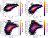 |
Fig. A.1. Band ratio F770W/F2100W grows with the Hα luminosity of the H II regions. This effect is seen for both observed (panel a) and stellar continuum subtracted (panel b) data in F770W. Panels c and d show the same line ratios after local background subtraction. The color denotes the number density of the regions, and the cyan curve represents a smoothed running median across the Hα luminosities. |
The brightness in all mid-IR bands considered here shows a tight semilinear correlation with the extinction-corrected Hα brightness (Leroy et al. 2023), which we also see in the integrated measurements for the H II regions. We find that subtraction of the local background does not affect this linear correlation but only leads to a systematic offset and a slight change in the slope of that correlation. Meanwhile, this removing background produces noticeable changes in F770W/F1130W and F770Wss/F1130W ratios: their dependence on log(Hα) has large scatter and becomes non-linear (Fig. A.1c,d), in contrast with those based on original flux measurements (panels a,b). In turn, this can result in stronger disagreement between the measurements RPAH and RPAH*, and therefore we provide a separate calibration for the background-subtracted version of RPAH* (see Appendix B). Meanwhile, background subtraction does not significantly affect the measurements of RPAH itself (and thus recalibrated version of RPAH*). Thus, Fig. A.2 demonstrate that RPAH* after background subtraction still shows the same strong correlation with log([SIII]/[SII]) as in Fig. 5, with a slightly larger scatter and small systematic offset (< 0.1 dex) relative to the linear trend defined by Eq. (4). Therefore, mostly to prevent an increase in the scatter, we use original measurements without background subtraction. Note, however, that the local background subtraction is crucial for interpretation of the comapact sources, such as SNRs (see Sec. 5.3).
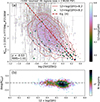 |
Fig. A.2. Same as Fig. 5c,d, but for RPAH* derived from the local background subtracted measurements. The background subtraction does not affect the conclusions made for H II regions. |
Appendix B: Calibration of RPAH* prescription
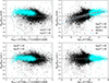 |
Fig. B.1. Ratio of two tracers of PAH mass fraction (RPAH and RPAH*) for ∼12000 H II regions from 19 PHANGS galaxies (top row) depending on RPAH (left panel) and monochromatic luminosity Lν(F770Wss) (right panel). Cyan and black denote regions with hydrogen ionizing photons rate Q0 > 1050 s−1 and Q0 < 1050 s−1, respectively. RPAH* and RPAH are consistent with each other for most of the regions, but RPAH* systematically overestimates PAH fraction for the luminous H II regions. The bottom row demonstrates the same ratio with RPAH* calculated after applying correction described in the text. |
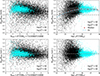 |
Fig. B.2. Same as Fig. B.1, but after removing the local background from the flux measurements in all involved JWST bands. |
Since F1130W-band images necessary for calculating RPAH are not available for most galaxies in our sample, we rely on RPAH* ∼ F770Wss/F2100W as a tracer of the PAH fraction. Sutter et al. (2024) demonstrated that RPAH* = 2.57 × F770Wss/F2100W provide a very good agreement with RPAH measurements when applied to diffuse ISM. Fig. A.1 shows that F770W/F1130W is not constant in the range of Hα luminosities considered here. Thus, here we refine RPAH* prescription from Sutter et al. (2024) against RPAH measurements to make it applicable for nebulae of different luminosities.
The top panels of Fig. B.1 shows how the ratio between original RPAH* (from Sutter et al. 2024 approximation) and RPAH changes with RPAH and F770W derived for our sample of H II regions from 19 PHANGS galaxies. In agreement with Sutter et al. (2024) findings for diffuse ISM, RPAH* yields very consistent values with RPAH when measured in relatively faint H II regions, and the typical scatter around the 1-to-1 relation is within 0.05 dex (< 12%). However, RPAH* is systematically higher (by ∼7 − 17%) than RPAH in bright star-forming regions H II regions. For example, cyan color in Fig. B.1 shows the regions more luminous than L(Hα)∼1 − 3 × 1038 erg s−1, which roughly corresponds to Q0 ∼ 1050 s−1, or an H II region ionized by 4–5 OV5 stars assuming no escape of ionizing photons. Most probably, this observed trend reflects the different band F1130W/F770W ratio (depending on the PAHs ionization or the radiation field spectrum) toward the bright and faint H II regions. Fig. A.1 (see also Egorov et al. 2023) shows that low F770W/F1130W tends to be observed preferentially in faint H II regions. Baron et al. (2025) revealed strong correlation between F1130W/F770W and [S II]/Hα, which also implies that higher values of F770W/F1130W are expected from the diffuse ISM (in general showing higher [S II]/Hα compared to the H II regions, Belfiore et al. 2022). Finally, Baron et al. (2025) found that some regions with anomalously low F770W/F1130W ratios also have elevated stellar-to-PAH ratios (i.e., F200W/F770W) different from those adopted by Sutter et al. (2024) for calculating F770Wss.
The top right panel of Fig. B.1 demonstrates that RPAH*/RPAH ratio correlates with a logarithm of monochromatic luminosity logLν(F770Wss) and can be well approximated by the second-order polynomial:
 (B.1)
(B.1)
Here the best-fit result is obtained with a2 = −0.00832 ± 0.00081, a1 = 0.4881 ± 0.0403, and a0 = −6.01 ± 0.52. The uncertainties are obtained as the standard deviation of the measured coefficients across 500 randomly bootstrapped samples, each comprising 2/3 of the original dataset. Dividing the RPAH* measurements by the Lν(F770Wss)-dependent multiplicative factor defined by this equation, we put them into agreement with RPAH across the entire range of RPAH and Lν(F770Wss) values and Hα luminosities (see bottom panels of Fig. B.1. Therefore, in this study we use the RPAH* refined in such a way (and thus derived with Eqs. (1, (2)).
Removing the local background changes the F770Wss (and thus Lν(F770Wss)) values and thus such a non-linear correction can be invalid when applied to the background-subtracted measurements. Indeed, Fig. B.2 shows the same distributions as in Fig. B.1, but for the measurements made after removing the local background. Unlike previously discussed, RPAH* prescription from Sutter et al. (2024) and RPAH measurements have a nearly constant multiplicative offset by a factor of ∼1.15 for the entire sample of H II regions. For consistency, we approximate it with the same second-order polynomial (Eq. (B.1)), but with different best-fit coefficients: a2 = −0.02009 ± 0.00141, a1 = 1.0597 ± 0.0736, and a0 = −12.81 ± 0.96. All RPAH* values relying on the background-subtracted measurements are calculated using these coefficients (namely, with Eqs. (1, 3).
Appendix C: Linking observational properties of H II regions with Cloudy models
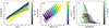 |
Fig. C.1. Dependence between different observational and physical parameters derived from the BOND models (Vale Asari et al. 2016) produced with the Cloudy photoionization code (Ferland et al. 2017). Panel a: log([SIII]/[SII]) vs the logarithm of the ionization parameter, log(U), color-coded with the age of the ionizing star cluster. log([SIII]/[SII]) strongly correlates with the ionization parameter, with the secondary dependence on the age. Panel b: log([SIII]/[SII]) vs logarithm of the outer size of the H II region, log(Rout), color-coded by the logarithm of the hydrogen ionizing photons rate, log(Q0). At the fixed value of the ionizing flux, the observed log([SIII]/[SII]) depends on the size of the region. Panel c: Dependence of F8μm/F24μm, similar to RPAH*, on the log([SIII]/[SII]). The existing Cloudy models can only partially reproduce the trend seen in Fig. 5. |
Similarly to Egorov et al. (2023), this study relies on the [S III]/[S II] emission lines ratio as a tracer of the ionization parameter (see, e.g., Diaz et al. 1991; Kewley et al. 2019). Based on photoionization models, here we demonstrate this dependence, as well as a secondary relation of this ratio on other physical properties considered in this study.
For simplicity, we considered existing “BOND” models (Vale Asari et al. 2016) accessible via the 3MdB database (Morisset et al. 2015). The photoionization model grids were produced using the Cloudy v17.01 code (Ferland et al. 2017) by varying the parameters of the cloud (its size and geometry, oxygen and nitrogen abundances) and ionizing source (age of the cluster and input ionization parameter) as described in Vale Asari et al. (2016). We only consider models with oxygen abundance 12 + log(O/H) = 7.6…9.0, ionization parameter log(U) = − 5…−1, and hydrogen density log(nH/cm−3) = 0…2.5 spanning the properties of the H II regions in this study.
Fig. C.1a shows that log([SIII]/[SII]) indeed linearly depends on the logarithm of the ionization parameter, although it also exhibits a clear secondary dependence on the age of the ionizing star cluster: the [S III]/[S II] ratio is typically lower for older regions of the same ionization parameter. As discussed in Sec. 4.2 and in Egorov et al. (2023), our interpretation of the observational dependence of the PAH fraction on the ionization parameter is unlikely to be biased by this secondary dependence on the age as we do not observe a correlation with other age-sensitive tracers like EW(Hα).
By definition, log U linearly depends on the logarithm of the hydrogen ionizing photons rate, log(Q0), and thus log([SIII]/[SII]) must do. This is indeed seen in Fig. C.1b. This plot also demonstrates that at constant ionizing photon rate (and thus mass and age of the ionizing cluster), larger H II regions exhibit lower [S III]/[S II] line ratio. This secondary dependence is a reason why the line-of-sight projection effect can be partially responsible for the observed correlation between RPAH and log([SIII]/[SII]) (see discussion in Sec. 4.2).
Cloudy code does not calculate all the chemical reaction taking place in the PDRs and depends on the input from the dedicated sub-grid models. By default, it considers simplified, but reasonable process of PAH destruction in H II regions: PAH fraction qPAH linearly decreases with the fraction of the ionized hydrogen, H+/(H+ + H0), at the particular radius. In turn, the ionization fraction directly depends on the number of the hydrogen ionizing photons available to ionize the ISM. PAH fraction in PDRs unaffected by the ionizing radiation is defined by the net chemical reactions depending on the dust content and size distribution, and thus related to the processes of the PAH formation rather then of their destruction. In principle, such a simplified picture is in qualitative agreement with our proposed interpretation of the observational results. Therefore, we expect to see in integrated Cloudy models a dependence between RPAH and [S III]/[S II] similar (although, not necessarily identical) to what is presented in Figs. 5. Figure C.1c shows such a dependence, where F8μm/F24μm (corresponding to the modeled brightness at Spitzer IRAC4/MIPS24 bands) is given as RPAH tracer. This tracer must produce qualitatively similar results to those obtained with RPAH*.
In Fig. C.1c, we indeed observe a similar decrease in IRAC4/MIPS24 with [S III]/[S II] to what is seen for the observed H II regions. However, there are several noticeable differences between these simple Cloudy models and the observations. The models exhibit much larger scatter of IRAC4/MIPS24 in the high-metallicity regime than RPAH or RPAH* in the observations, with some region having almost no surviving PAHs even for low values of the [S III]/[S II] ratio. Furthermore, the metallicity dependence is noticeable in this plot, while it is absent in the observational results. Similarly to the observations, the Cloudy models reproduce a different behavior of the PAH fraction tracer with [S III]/[S II] in the low-metallicity regime (12 + log(O/H) < 8.2), however, the resulting PAH fraction in the models is significantly higher than in the observations (especially for high [S III]/[S II] ratio). Therefore, despite the qualitative agreement, the real evolution of PAHs around H II regions is more complex and PAH destruction is unlikely just linearly dependent on the ionization fraction as assumed in the Cloudy models.
Appendix D: Online catalog
We report most of the measurements used or derived in this work in the online table accessible at the CDS. A list of the columns included in the catalog is provided in Table D.1. The table contains information on 17151 H II regions and 396 SNRs selected according to the S/N and environmental criteria presented in Sections 3.1 and 3.2. The parent samples of H II regions and SNRs for the 19 PHANGS-MUSE galaxies are taken from the catalogs of Groves et al. (2023) and Li et al. (2024), respectively. The full catalog of H II regions for 23 additional galaxies will be published in future work (Egorov et al., in prep.). The exact identification of H II regions in that work may differ from what is presented here.
Columns in the catalog accessible at the CDS.
All Tables
All Figures
|
Fig. 1. Distribution of log(RPAH*) vs. oxygen abundance color-coded by log([SIII]/[SII]) (tracer of the ionization parameter) for all H II regions in the sample. The red circles show the average values in different metallicity bins (reported in Table 2). The vertical gray dashed line marks 12 + log(O/H) = 8.2 as a threshold between the low- and high-metallicity regimes. The horizontal dashed line corresponds to the average RPAH for diffuse ISM measured by Sutter et al. (2024). The black squares correspond to measurements for WLM and NGC6822 (from low- to high-metallicity) made by (Chown et al. 2025a) using JWST F770W and F2100W images. The PAH fraction drops significantly in the low-metallicity regime. |
| In the text | |
|
Fig. 2. Distribution of RPAH* vs. oxygen abundance for the entire sample of H II regions (gray histogram with intensity tracing the probability density), and average distribution for two bins in log([S III]/[S II]). The dashed lines are the same as in Fig. 1. The black squares represent measurements for WLM, NGC6822 (as in Fig. 1), the SMC, and the LMC from Chown et al. (2025a), listed in order of increasing metallicity. Spitzer IRAC4 and MIPS24 filters were used to estimate RPAH* for the SMC and LMC (Chown et al. 2025a). |
| In the text | |
|
Fig. 3. RPAH* (see color bar at right) calculated on the regularly distributed bins with unique O/H and [S III]/[S II] values. The metallicity and ionization parameters are both important for setting up the PAH fraction. |
| In the text | |
|
Fig. 4. Distribution of RPAH* for resolved (luminous) H II regions (orange) and the regions of similar size from the diffuse ISM (blue) for several gas-phase metallicity bins. The one dashed line and the two dotted lines on each distribution show the median and 25 and 75 percentile quartiles, respectively. Both RPAH and RPAH* are lower in the H II regions than in the diffuse ISM. A strong decrease in RPAH* in the lowest metallicity bin is seen for the H II regions and the diffuse ISM. |
| In the text | |
|
Fig. 5. PAH fraction anti-correlates with log([S III]/[S II]) (ionization parameter tracer) for thousands of H II regions in 42 PHANGS-JWST galaxies. Panels (a, b) shows all ∼17 200 analyzed H II regions, while the ∼5600 brightest resolved H II regions are shown in panels (c, d). The dashed red line shows the best-fit linear regression to the resolved sample defined by Eq. (4). The histograms in panels (b, d) show how the logarithmic residuals after subtracting this linear trend depend on metallicity. The color in panels (a, c) denotes gas-phase oxygen abundance; the red contours show the probability density of the high-metallicity (12 + log(O/H) > 8.2) points; the levels correspond to 50, 65, 80, 95, and 99 percentile intervals. The Spearman correlation coefficient (ρ) and RMS scatter around the linear fit are reported in panels (a, c). |
| In the text | |
|
Fig. 6. Same as Fig. 2, but here the blue and red curves correspond to different bins of low and high [O III]/Hβ (panel a) or [S II]/Hα (panel b), respectively. The orange curve and points are translated from the average values per metallicity bin in Fig. 4 in Whitcomb et al. (2024). |
| In the text | |
|
Fig. 7. About 45% of the RPAH measurements are overestimated by more than 10% when measured in the MUSE-based apertures for H II regions compared to the values in their centers. Panel (a) shows the probability distribution of RPAH measured in different circular apertures for the same sample of H II regions related to the value of RPAH measured at the local peaks of Hα brightness within the H II region. Panel b demonstrate how such ratios change for different Hα luminosity bins. The different colors correspond to different outer radii of the circular aperture. |
| In the text | |
|
Fig. 8. Histograms showing distribution of RPAH vs. the logarithm of the circularized radii of the H II regions derived from HST data (from Barnes et al. 2025; panel (a)), and vs the ionization parameter tracer log([SIII]/[SII]) (panel (b)). The colors denote the number of regions in each bin. The curved dashed, solid, and dotted lines in panel (a) show models defined by Eq. (5) with the disk scale height hd = 50, 100, and 400 pc, respectively. The red dashed line in panel (b) corresponds to Eq. (4). The anti-correlation between RPAH and the size of the H II region is much weaker than that with the ionization parameter, and can be partially explained by the contribution of the PAHs from the diffuse ISM along the line of sight. |
| In the text | |
|
Fig. 9. Distribution of RPAH vs. log([SIII]/[SII]) for the resolved H II regions (gray points; as in Fig. 5c) and isolated SNRs (red points). Panels (a) and (b) correspond to RPAH measurements from the observed and the local background subtracted fluxes. The black dashed line corresponds to the relation defined by Eq. (4). The cyan contours show the probability density distribution for H II regions; the levels correspond to 65, 80, 95, and 99 percentile intervals. |
| In the text | |
|
Fig. 10. Same as Fig. 4, but for SNRs (orange) compared to the diffuse ISM (blue). Panels (a) and (b) correspond to RPAH measurements from the observed and the local background subtracted fluxes. SNRs do not reveal a decrease in RPAH measured from the observed fluxes indicating that SN shocks are unlikely major contributors to the selective PAH destruction at 50 pc scale. A more localized effect is evident from the background-subtracted measurements. |
| In the text | |
|
Fig. A.1. Band ratio F770W/F2100W grows with the Hα luminosity of the H II regions. This effect is seen for both observed (panel a) and stellar continuum subtracted (panel b) data in F770W. Panels c and d show the same line ratios after local background subtraction. The color denotes the number density of the regions, and the cyan curve represents a smoothed running median across the Hα luminosities. |
| In the text | |
|
Fig. A.2. Same as Fig. 5c,d, but for RPAH* derived from the local background subtracted measurements. The background subtraction does not affect the conclusions made for H II regions. |
| In the text | |
|
Fig. B.1. Ratio of two tracers of PAH mass fraction (RPAH and RPAH*) for ∼12000 H II regions from 19 PHANGS galaxies (top row) depending on RPAH (left panel) and monochromatic luminosity Lν(F770Wss) (right panel). Cyan and black denote regions with hydrogen ionizing photons rate Q0 > 1050 s−1 and Q0 < 1050 s−1, respectively. RPAH* and RPAH are consistent with each other for most of the regions, but RPAH* systematically overestimates PAH fraction for the luminous H II regions. The bottom row demonstrates the same ratio with RPAH* calculated after applying correction described in the text. |
| In the text | |
|
Fig. B.2. Same as Fig. B.1, but after removing the local background from the flux measurements in all involved JWST bands. |
| In the text | |
|
Fig. C.1. Dependence between different observational and physical parameters derived from the BOND models (Vale Asari et al. 2016) produced with the Cloudy photoionization code (Ferland et al. 2017). Panel a: log([SIII]/[SII]) vs the logarithm of the ionization parameter, log(U), color-coded with the age of the ionizing star cluster. log([SIII]/[SII]) strongly correlates with the ionization parameter, with the secondary dependence on the age. Panel b: log([SIII]/[SII]) vs logarithm of the outer size of the H II region, log(Rout), color-coded by the logarithm of the hydrogen ionizing photons rate, log(Q0). At the fixed value of the ionizing flux, the observed log([SIII]/[SII]) depends on the size of the region. Panel c: Dependence of F8μm/F24μm, similar to RPAH*, on the log([SIII]/[SII]). The existing Cloudy models can only partially reproduce the trend seen in Fig. 5. |
| In the text | |
Current usage metrics show cumulative count of Article Views (full-text article views including HTML views, PDF and ePub downloads, according to the available data) and Abstracts Views on Vision4Press platform.
Data correspond to usage on the plateform after 2015. The current usage metrics is available 48-96 hours after online publication and is updated daily on week days.
Initial download of the metrics may take a while.