| Issue |
A&A
Volume 704, December 2025
|
|
|---|---|---|
| Article Number | A218 | |
| Number of page(s) | 37 | |
| Section | Stellar structure and evolution | |
| DOI | https://doi.org/10.1051/0004-6361/202554786 | |
| Published online | 12 December 2025 | |
Populations of evolved massive binary stars in the Small Magellanic Cloud
I. Predictions from detailed evolution models
1
Argelander-Institut für Astronomie, Universität Bonn, Auf dem Hügel 71, 53121 Bonn, Germany
2
Max-Planck-Institut für Radioastronomie, Auf dem Hügel 69, 53121 Bonn, Germany
3
Max-Planck-Institut für Astrophysik, Karl-Schwarzschild-Strasse 1, 85748 Garching, Germany
4
Tel Aviv University, The School of Physics and Astronomy, Tel Aviv 6997801, Israel
5
Instituto de Astrofísica de Canarias, 38200 La Laguna, Tenerife, Spain
6
Dpto. Astrofísica, Universidad de La Laguna, 38205 La Laguna, Tenerife, Spain
7
Max-Planck-Institut für Extraterrestrische Physik, Gießenbachstraße 1, 85748 Garching, Germany
8
Steward Observatory, Department of Astronomy, University of Arizona, 933 N. Cherry Ave., Tucson, AZ 85721, USA
9
Department of Physics and Astronomy, Krijgslaan 281/S9, 9000 Gent, Belgium
10
Department of Materials and Production, Aalborg University, Fibigerstræde 16, 9220 Aalborg, Denmark
★ Corresponding authors: This email address is being protected from spambots. You need JavaScript enabled to view it.
; This email address is being protected from spambots. You need JavaScript enabled to view it.
; This email address is being protected from spambots. You need JavaScript enabled to view it.
Received:
27
March
2025
Accepted:
7
August
2025
Abstract
Context. The majority of massive stars are born with a close binary companion. How this affects their evolution and fate is still largely uncertain, especially at low metallicity.
Aims. We derive synthetic populations of massive post-interaction binary products and compare them with corresponding observed populations in the Small Magellanic Cloud (SMC).
Methods. We analyse 53298 detailed binary evolutionary models computed with MESA. Our models include the physics of rotation, mass and angular momentum transfer, magnetic internal angular momentum transport, and tidal spin-orbit coupling. They cover initial primary masses of 5–100 M⊙, initial mass ratios of 0.3–0.95, and all initial periods for which interaction is expected, 1–3162 d. They are evolved through the first mass transfer and the donor star death, and a a possible ensuing Be X-ray binary phase, and they end when the mass gainer leaves the main sequence.
Results. In our fiducial synthetic population, 8% of the OB stars in the SMC are post-mass-transfer systems, and 7% are merger products. In many of our models, the mass gainers are spun up and expected to form Oe/Be stars. While our model underpredicts the number of Be X-ray binaries in the SMC, it reproduces the main features of their orbital period distribution and the observed number of SMC binary WR stars. We further expect ∼50 OB+BH binaries below and ∼170 above the 20 d orbital period. The long-period OB+BH binaries might produce merging double black holes. However, their progenitors, the predicted long-period WR+OB binaries, are not observed.
Conlcusions. While the comparison with the observed SMC stars supports many physics assumptions in our high-mass binary models, a better match for the large number of observed OBe stars and Be X-ray binaries likely requires a lower merger rate and/or a higher mass transfer efficiency during the first mass transfer. The fate of the initially wide O star binaries remains particularly uncertain.
Key words: stars: black holes / stars: emission-line, Be / stars: neutron / stars: Wolf-Rayet / Magellanic Clouds / X-rays: binaries
© The Authors 2025
 Open Access article, published by EDP Sciences, under the terms of the Creative Commons Attribution License (https://creativecommons.org/licenses/by/4.0), which permits unrestricted use, distribution, and reproduction in any medium, provided the original work is properly cited.
This article is published in open access under the Subscribe to Open model. This email address is being protected from spambots. You need JavaScript enabled to view it. to support open access publication.
1. Introduction
A new window onto the Universe was opened by the first direct detection of gravitational waves, emitted by the merging of two stellar-mass black holes (BHs; Abbott et al. 2016). Up to now, more than 100 compact object merger events have been detected in this way (Abbott et al. 2023). Several formation channels have been proposed (Belczynski et al. 2016; Mapelli 2020; Mandel & Broekgaarden 2022), including the formation of double compact objects in isolated massive binaries. Due to the cosmological distance of these sources, and considerable delay times between the compact object formation and the merger, many of them will have formed in the low-metallicity environment of the high-redshift Universe (Belczynski et al. 2016; Klencki et al. 2025).
An understanding of the formation of tight double-compact binaries through binary evolution is intimately linked to an understanding of massive stars, since most of them are born with a close companion with which they will interact (Sana et al. 2012). Massive star feedback, be it via emitting newly synthesized chemical elements, kinetic energy, or ionizing radiation, is strongly affected by the presence of a companion (Zapartas et al. 2017; Götberg et al. 2019; Eldridge & Stanway 2022), which is therefore important for the evolution of star-forming galaxies (Ma et al. 2016; Fichtner et al. 2022).
While this holds for all redshifts, we can study metal-rich individual massive stars and binaries in detail. Galaxies are observed at redshifts beyond 14 (Carniani et al. 2024; Helton et al. 2025), and individual stars in these galaxies cannot be resolved. In this respect, the Small Magellanic Cloud (SMC) provides an ideal laboratory in which to investigate massive single-star and binary evolution at conditions prevalent in the early Universe. Its metallicity of only ∼1/5 the solar one (Hill et al. 1995; Korn et al. 2000; Davies et al. 2015) corresponds to the average metallicity of star-forming galaxies at a redshift of ≈5 (Langer & Norman 2006). Yet, with a distance of only 61.9 ± 0.6 kpc (de Grijs & Bono 2015), and with a current star formation rate of ∼0.05 M⊙ yr−1 (Harris & Zaritsky 2004; Rubele et al. 2015; Hagen et al. 2017; Rubele et al. 2018; Schootemeijer et al. 2021), it shows us a rich population of massive stars.
The SMC is also an ideal test bed for massive star evolution for other reasons. Firstly, due to its low metallicity, the wind loss of hot stars is weak (Mokiem et al. 2007), such that the uncertainty in their mass and angular momentum loss is reduced. Secondly, the extinction towards most of the stars is very low (Górski et al. 2020). Except for potentially the youngest massive stars (Schootemeijer et al. 2021), it is thus generally assumed that we observe their complete populations, which makes the SMC well suited for population synthesis studies. The BLOeM survey will provide further information about the binarity of the SMC massive stars, offering critical tests for binary evolution models (Shenar et al. 2024).
Figure 1 presents a schematic picture of the evolutionary phases of massive close binary systems, up to the time where the initially less massive star leaves the main sequence. It demonstrates that binary evolution models may be compared with the properties of several observed populations of evolved massive binaries in the SMC. While so far, 14 radio pulsars are known in the SMC (Carli et al. 2024) of which 1 has a B star companion, the SMC’s massive X-ray binary population is particularly rich, with about 150 objects, of which ∼100 are identified to be Be X-ray binaries (BeXBs, Haberl & Sturm 2016). Furthermore, Schootemeijer et al. (2022) identified more than 1700 OBe stars brighter than MV ≃ −3 mag (≳9 M⊙), most of which are thought to represent spun-up mass gainers in binary systems (Shao & Li 2014; Bodensteiner et al. 2020). Drout et al. (2023), by searching for UV excess, identified nine hot stars in the SMC with high surface gravities, consistent with the expectation for stars stripped in binaries. The SMC also harbours 12 Wolf-Rayet (WR) stars, four of which show a close OB star companion (Shenar et al. 2016; Neugent et al. 2018).
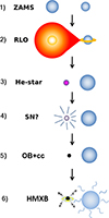 |
Fig. 1. Schematic evolution of a massive binary system through the six evolutionary phases considered in this paper: pre-interaction, RLO, stripped envelope star (subdwarf, helium star, or Wolf-Rayet star), compact object, referred to as the compact companion (cc) in a binary system, formation possibly connected with a SN explosion, X-ray silent compact object binary, and HMXB. After the second stage, a fraction of the mass gainers may be fast-rotating and appear as Oe or Be stars, and after NS formation as a OBe X-ray binary. Notably, many systems do not survive the second, fourth, and sixth stage as a binary, i.e. the number of systems evolving from top to bottom is being reduced at these stages. The figure is adapted from Kruckow et al. (2018). |
While the predictions of population synthesis models can be compared with these observed samples of post-interaction binaries, for several binary evolutionary stages we basically lack any observed counterparts. This holds in particular for rich predicted populations of stripped mass donors that lack the strong winds to make them appear as WR stars (Wellstein et al. 2001; Götberg et al. 2018; Langer et al. 2020a; Shenar et al. 2020; Drout et al. 2023), for wind accreting BHs with OB star companions (Shao & Li 2019; Langer et al. 2020b; Janssens et al. 2022), which may lack observable X-ray emission (Hirai & Mandel 2021; Sen et al. 2021, 2024), very few of which are known in the Galaxy and Large Magellanic Cloud (LMC) (Orosz et al. 2009, 2011; Shenar et al. 2022a; Mahy et al. 2022), and none of which have been found so far in the SMC. Here, population synthesis predictions are useful to refine targeted searches for such objects.
We aim to provide predictions for the evolved phases of massive binary stars in the SMC based on detailed MESA binary evolution models. This work covers all the evolutionary stages presented in Fig. 1. The later stages up to the merger of binary BHs will be investigated in our follow-up work by using the population derived in this work and our detailed model data. Our work is closely related to that of Schürmann et al. (2025; hereafter Paper II), who undertake a similar effort using the rapid binary evolution code ComBinE (Kruckow et al. 2018). Our paper is organized as follows. In Sect. 2, we introduce the grid of detailed binary evolution models used for our analysis, and detail the essential input physics. In Sect. 3, we present the results of our fiducial population synthesis model, and in Sect. 4 we describe the results of parameter variations. In Sect. 5, we compare our results with observations. We discuss the key uncertainties in our calculations in Sect. 6, before summarizing our results in Sect. 7.
2. Method
This work is based on a dense grid of detailed massive binary evolution models (Wang et al. 2020), which was calculated with the one-dimensional stellar evolution code MESA (Modules for Experiments in Stellar Astrophysics version 8845) using a tailored metallicity appropriate for the SMC, as in Brott et al. (2011). The detailed description of this code can be found in Paxton et al. (2011, 2013, 2015). Using statistical weights depending on the initial distributions and lifetimes allows us to perform population synthesis.
In contrast to rapid binary population synthesis, where different binary model parameters can easily be explored, we only have one fixed binary evolution grid to work with. However, in order to construct a synthetic population from that model grid, parameters are introduced, which can be varied later on. This concerns in particular the birth kicks of compact objects, the core mass ranges defining the emerging compact object type, the threshold rotation for assuming an OBe nature, and the star formation history. In the following subsections, we describe our method in detail.
2.1. Input physics
Here we briefly summarize our input physics parameters for the MESA calculations. In order to model convection, the standard mixing length theory is adopted with a mixing length parameter of αMLT = 1.5 (Böhm-Vitense 1958). We used the Ledoux criterion to identify convective layers, and adopted step-overshooting for the hydrogen-burning core using a parameter αov = 0.335 (Brott et al. 2011). We modelled semiconvection according to Langer et al. (1983) using a semiconvection efficiency parameter of αsc = 1 (Langer 1991; Brott et al. 2011; Schootemeijer et al. 2019). We follow Cantiello & Langer (2010) in modelling thermohaline mixing with the efficiency parameter αth = 1. Rotation-induced mixing was computed in the diffusion approximation as in Heger & Langer (2000), including the dynamical (Endal & Sofia 1978) and secular shear instability (Maeder 1997), Goldreich-Schubert-Fricke instability (Goldreich & Schubert 1967; Fricke 1968) and Eddington-Sweet circulation (Eddington 1929). In addition, the Spruit-Taylor dynamo was included for the internal angular momentum transport (Spruit 2002).
We adopted stellar wind mass loss following the treatment in Brott et al. (2011), which includes the so-called bi-stability jump (Vink et al. 1999). The first jump is near an effective temperature of 22 kK, below which the mass-loss rate was computed according to Nieuwenhuijzen & de Jager (1990) and Vink et al. (2000, 2001). This mass-loss prescription may need revisions, as recent observations on galactic massive stars do not find evidence for the changes in mass-loss rates across the jump temperature (de Burgos et al. 2024). For enhanced surface helium abundances, with helium mass fractions in the range 0.3–0.7, the mass-loss rate was smoothly increased towards empirical WR rates (Hamann et al. 1995). In addition, enhanced mass loss by rotation was assumed as in Heger & Langer (2000). While rotation does not necessarily enhance mass loss (Hastings et al. 2023), the purpose of this assumption in our models was to prevent the accreting components in mass transfer models from achieving faster-than-critical rotation. Stellar wind also carries away angular momentum, braking stellar rotation. During each time step, our model (MESA ver. 8845) calculated the angular momentum loss by removing the angular momentum contained in the removed layer, which was done the same way as in Brott et al. (2011). Assuming a constant surface specific angular momentum during one time step, which appears to be more physically correct and is done in the most recent MESA versions, would result in a stronger wind induced spin-down than our scheme, and would thus lead to a smaller number of OBe stars (cf. Paper II). However, as (Nathaniel et al. 2025) find that the spin-down of Galactic O stars appears to be better reproduced with the old angular momentum loss prescription, we consider this issue unresolved.
We considered only circular orbits. The orbital evolution of our binary models is affected by mass transfer (Tauris & van den Heuvel 2023) and tides (Hut 1981; Hurley et al. 2002; Sepinsky et al. 2007). We used the Hut_rad scheme coded in MESA to calculate radiative-damping dominated tidal interaction (Detmers et al. 2008), while recently Sciarini et al. (2024) argue that there could be inconsistency in this tide prescription. Mass transfer takes place when the radius of the primary star exceeds the radius of its Roche lobe, where the Roche lobe radius was calculated with the analytic fit derived by Eggleton (1983). In order to account for long-term contact phases, the contact scheme in MESA was adopted (Marchant et al. 2016; Menon et al. 2021). During mass transfer, accretors can be spun up to critical rotation (Packet 1981; Petrovic et al. 2005). The accretor was assumed to accrete as much as possible before reaching critical rotation. When the expected mass transfer rate would cause it to exceed critical rotation, we assumed the accretor can only accrete the amount that makes it remain below critical rotation (Petrovic et al. 2005), which sets a balance among tidal interaction, accretion, and structure adjustment that gives the mass transfer efficiency in a self-consistent way (Paxton et al. 2015). The non-accreted material was assume to be ejected from the binary system, carrying the specific orbital angular momentum of the mass gainer (so-called isotropic re-emission; Soberman et al. 1997). This leads to a rotation-dependent accretion efficiency. In wide-orbit binaries, where tides are inefficient, the accretion efficiency is often below 10%, while it can reach 60% in narrow-orbit binaries.
We setted an upper limit on the mass loss rate from the binary system, Ṁlimit, by comparing the photon luminosity of the stars with the energy input rate that is required to maintain the current mass-loss rate from the binary, as Marchant (2017):
 (1)
(1)
Here, L1 and L2 are the luminosities of the mass donor and the mass gainer, M2 is the mass of mass gainer, and RL, 2 is the Roche-lobe radius of the mass gainer, at which material is assumed to be ejected. If a larger mass-loss rate from the binary system is required, we assumed that the mass transfer is unstable and produces a binary merger. With the above condition, the critical mass ratio for unstable mass transfer in our models is sensitive to the initial orbital period and the initial primary mass of the system (see Sect. 2.2 and Fig. 2). The merger rate based on Eq. (1) is a lower limit, as the ejection of the same amount of material at other locations, like the surface of the mass gainer or the accretion disc around the mass gainer, would require higher radiation energies, resulting in a lower threshold for the mass-loss rate from the system. In addition, we also assumed unstable mass transfer if the mass transfer rate exceeds 0.1 M⊙ yr−1, if inverse mass transfer occurs with a post-main-sequence (post-MS) donor, or if the second Lagrangian point (L2) overflow occurs during a contact phase. The survivors of unstable mass transfer were ignored, as their initial parameter space is narrow (e.g. Ercolino et al. 2024) and expected to take a small fraction of the population considered in this work.
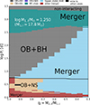 |
Fig. 2. Outcome of the first mass transfer phase in our detailed binary evolution models with an initial primary mass of 17.8 M⊙. In this figure, each pixel represents one detailed MESA binary evolution model, and the corresponding evolutionary outcome is colour-coded (see top legend). Here, ‘OB+cc’ (cc= BH, NS, WD) implies that the corresponding model produced an OB+cc phase, with the cc type indicated by the corresponding colour. However, depending on the adopted compact object birth kicks, these systems may also break up. Systems indicated as ‘Upper_mdot_limit’ or ‘MT_max’ are terminated during their first mass transfer phase as the mass transfer rate exceeds limiting values (see text) and a merger is expected, and those indicated as ‘other merger’ undergo L2-overflow in a contact situation. Corresponding plots for different initial donor star masses can be found in Appendix A. |
Our binary models were evolved from the zero-age main-sequence (ZAMS) stage up to core carbon depletion of the primary star, except for donor stars with a helium core mass above 13 M⊙, for which we terminated the evolution at core helium depletion for numerical reasons. After the termination of the primary star, we further evolved the secondary star as a single star. This numerical setting allows one to explore various post-supernova (post-SN) scenarios (cf. Sects. 2.5 and 2.6).
2.2. Binary model grid
Our SMC binary model grid (Wang et al. 2020) contains 53298 detailed evolution models. The model data1 and necessary files2 to reproduce our models are available online. We assumed that the stars are initially tidally locked. Therefore, the initial binary parameters are the initial primary mass, M1, i, initial mass ratio, qi, and initial orbital period, Porb, i. Our model grid was computed with the following parameter space:
-
Initial primary masses, M1, i, were set in the range of 5–100 M⊙, or log (M1, i/M⊙) between 0.7 and 2, with constant intervals of Δ log(M1, i/M⊙) = 0.05;
-
Initial mass ratios, qi, were considered between 0.3 and 0.95 with a constant interval of Δ qi = 0.05;
-
Initial orbital periods, Porb, i, were selected from 1 d to 3162 d, or log(Porb, i/day) = 0.0–3.50, with constant intervals of Δ log (Porb, i/day) = 0.025.
The input parameter space covers all initial primary masses of BH and neutron star (NS) progenitors below 100 M⊙ and all initial orbital periods for interacting systems. The lower limit on the initial mass ratio was chosen to be 0.3, below which we expect mass transfer to be unstable (Soberman et al. 1997). While recent studies (Ge et al. 2020; Marchant et al. 2021; Schürmann & Langer 2024) find that stable mass transfer is possible for qi < 0.3 in the long-period regime, the corresponding parameter space is small and can be neglected for the purpose of this study.
Figure 2 provides an overview of the models, and the outcome of the first mass transfer phase, for all models with an initial primary mass of M1, i = 17.8 M⊙ (see Appendix A for other initial primary masses). According to the definition of Kippenhahn & Weigert (1967), our closest binaries undergo Case A mass transfer, where the primary star fills its Roche lobe during its core hydrogen burning phase. Above an initial orbital period of ∼5 d, the mass transfer takes place with a shell hydrogen burning donor (Case B mass transfer). At this initial primary mass, our Case A mass donors form NSs, and our Case B mass donors form BHs, according to our adopted maximum final He-core mass limit of 6.6 M⊙ for NS formation (cf. Sect. 2.5). For initial orbital periods above ∼300 d, the mass transfer rate violates our upper limit of 0.1 M⊙ yr−1. Here, mass transfer was expected to become unstable due to the convective envelope of the donor star (Soberman et al. 1997). The widest binaries do not experience any binary interactions and serve as a grid of single star models.
Based on our stability criterion from Eq. (1), we find that a large fraction of models undergo unstable mass transfer (labelled by ‘Upper_mdot_limit’ in Fig. 2). For higher initial primary masses, fewer binary models experience unstable mass transfer (cf. Figs. 2, A.1, and A.2). Also, the Case A/B boundary is shifted to larger initial orbital periods, even exceeding 1000 d for the highest initial primary mass, due to envelope inflation near the Eddington limit (Sanyal et al. 2015, 2017; Sen et al. 2023).
If unstable mass transfer occurs during a Case A mass transfer, the merger product is expected to be a MS star, and we followed its evolution by using the merger models at the SMC metallicity computed by Wang et al. (2022). In these models, the mass of the merger product, Mmerger, was determined by (Glebbeek et al. 2013)
, \end{aligned} $$](/articles/aa/full_html/2025/12/aa54786-25/aa54786-25-eq2.gif) (2)
(2)
where M1 and M2 are the masses of the primary and secondary stars at the time of the merger, and q = M2/M1. The ejected mass during merger is below 7.5% (q = 1) of the mass of the pre-merger system. This equation is based on a head-on collision, and less mass ejection can be expected for a gentler merger process (Schneider et al. 2016). The ejected material was assumed to be envelope material, which has the initial composition of the two stars.
The angular momentum content of merger stars is uncertain. While the available orbital angular momentum exceeds the possible angular momentum content of the merger product, angular momentum can be lost efficiently along with the ejected fraction of the total mass. Schneider et al. (2019) find, in detailed 3D MHD and 1D stellar simulations, that the product of a merger between two massive main-sequence (MS) stars is in fact slowly rotating due to angular momentum loss and thermal relaxation. We therefore assumed the same for our merger products, which implies in particular that they do not contribute to the predicted population of OBe stars.
2.3. OBe stars
The Be phenomenon is produced by rapidly rotating massive MS stars that show the Hα line in emission, and that have an spectral energy distribution showing an infrared excess. Both features are thought to originate from a circumstellar decretion disc that is fed from the layers near the stellar equator (Reig 2011; Rivinius et al. 2013). While Be stars are fast rotators, it is unclear how close they are to their critical rotation. Townsend et al. (2004) suggested that considering gravity darkening, all Be stars spin near their critical rotation. However, the concept of critical rotation is difficult to define (Hastings et al. 2023), and observations seem to imply that some Be stars can rotate sub-critically, with rotational velocities as low as ∼60% of the critical value (e.g. Huang et al. 2010; Zorec et al. 2016; El-Badry et al. 2022; Dufton et al. 2022).
In our fiducial model, we defined Be stars as rotating faster than 0.95 of their critical rotational velocities (υcrit). Golden-Marx et al. (2016) showed that Oe stars are the high-mass extension of Be stars, and therefore we adopted the same threshold value to define Oe stars. Since our spun-up accretors generally reach critical rotation, and keep it up during their further MS evolution (e.g. Hastings et al. 2020), the threshold value only affects the massive accretors that may slowly spin down due to their stellar wind (above ∼40 M⊙; Langer 1998). We quantify the effect of different threshold values in Sec. 4. We did not consider the detailed properties of the circumstellar discs (cf. Rubio et al. 2025).
2.4. Helium stars and Wolf-Rayet stars
Following the common nomenclature, we defined helium stars (He-stars) as stripped-envelope core helium burning stars (Shenar et al. 2020; Wang et al. 2021), whose winds remain optically thin, such that they will not show emission lines in their spectra. Conversely, we spoke of our model corresponding to a WR star when we can assume that it forms an optically thick stellar wind. Shenar et al. (2020) find a metallicity-dependent luminosity threshold for the WR phenomenon, as log L/L⊙ ≈ 4.9, 5.25, and 5.6 for the Galaxy, the LMC, and the SMC, respectively. Aguilera-Dena et al. (2022) and Sen et al. (2023) show that these luminosity limits are roughly reproduced by simple wind models, using the mass-loss rates as adopted here. Accordingly, we assumed that our stripped stars with log L/L⊙ > 5.6 correspond to WR stars. This limit is exceeded by He-stars above ∼15 M⊙, which requires initial masses above ∼40 M⊙. In addition, we defined hydrogen-free (H-free) WR stars by a surface hydrogen mass fraction of less than 0.05, according to the typical uncertainties of the observationally derived hydrogen abundances in Shenar et al. (2016).
2.5. Formation of compact objects
We adopted the types of compact objects formed by our donor stars according to their final model properties. Sukhbold et al. (2018) perform detailed simulations on the explodability of stars. They find a sudden increase in the compactness parameter of pre-supernova (pre-SN) stars at a final He core mass of 6.6 M⊙, which marks the formation of BHs. While stellar winds at different metallicities could alter the evolution of He stars (e.g. Wang & Han 2010; Doherty et al. 2015; Aguilera-Dena et al. 2022; Guo et al. 2024), the relation between the compactness parameter and the final He core mass is insensitive to metallicity (Sukhbold et al. 2016). Accordingly, we assumed that a BH forms if the final mass of a helium core MHe, c reaches 6.6 M⊙. For simplicity, the non-monotonous behaviour of the compactness parameter (O’Connor & Ott 2011; Sukhbold et al. 2016, 2018; Schneider et al. 2023; Aguilera-Dena et al. 2023) was ignored, and this assumption may overestimate the number of low-mass BHs. Different assumptions on mixing process can affect the explodability of stars by changing the final core carbon abundance (Patton & Sukhbold 2020; Schneider et al. 2021), resulting in different values of the mass threshold. This can affect the predicted number of low-mass BH but has a small effect otherwise (Janssens et al. 2022). The mass of the BH was computed by using the same assumption as in the ComBinE code (Kruckow et al. 2018, and Paper II), which is that 20% of the mass of the He-rich envelope of the core He depleted star is ejected, and after that 20% of the remaining mass is lost due to the release of gravitational binding energy.
Stars with very massive helium cores become unstable due to the production of electron–positron pairs. Those not massive enough to form a pair-production SN (Heger & Woosley 2002; Langer et al. 2007) undergo a series of energetic pulses accompanied by strong mass ejections (Heger & Woosley 2002; Chatzopoulos & Wheeler 2012; Woosley 2017; Marchant et al. 2019). This process is known as pulsational pair-instability (PPI). Marchant et al. (2019) simulate these mass ejections during the PPI with the MESA code. Base on their result, we performed a polynomial fitting to the helium core mass at core helium depletion and the remaining mass, Mrem, after the pulsations, which is3
 (3)
(3)
where Mrem and MHe,c are in the unit of solar mass. Figure 3 provides a comparison between our fitting formula and the model data in Marchant et al. (2019). This formula is only valid for 35.3 M⊙ ≤ MHe, c ≤ 61.1 M⊙. This mass range is somewhat sensitive to key nuclear reaction rates (Takahashi 2018; Farmer et al. 2020), for which current best estimates lead to a slightly higher mass range (e.g. Farag et al. 2022).
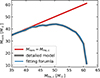 |
Fig. 3. Remaining mass, Mrem, after the pulsations triggered by pair instability, as a function of the helium core mass, MHe, c, at core helium depletion. The grey and blue lines correspond to the model data in Marchant et al. (2019) and Eq. (3), respectively. The red line shows the relation Mrem = MHe, c. |
We assumed that stars with final helium core masses below 6.6 M⊙ form NSs or, for stars with final carbon core masses below 1.37 M⊙ form WDs. The masses of our NSs were fixed to be 1.4 M⊙. Neutron star formation is accompanied by a SN explosion due to the collapsing core. Core collapse in the lowest-mass SN progenitors may be triggered by electron captures, producing a so-called electron-capture SN (ECSNe, Nomoto 1984; Tauris et al. 2015). Since the low-mass progenitors are expected to produce a weak momentum kick on the newborn NSs (Janka 2012), they play an important role in the formation of BeXBs (Podsiadlowski et al. 2004). However, our model grid cannot resolve the narrow mass range of ECSNe well (see Sect. B). For consistency with the results obtained with the ComBinE code (Paper II), we applied the SN scheme adopted in Kruckow et al. (2018) (see Appendix B for details). This considers four types of SNe:
-
Ordinary iron core collapse SNe (CCSNe), if the pre-SN star has a final carbon core mass larger than 1.435 M⊙ and a H-rich envelope;
-
H-envelope-stripped iron-core collapse SNe (CCSN-He) if the H-rich envelope has been stripped by mass transfer;
-
He-envelope-stripped iron-core collapse SNe (CCSN-C) if most of the He-rich envelope has been stripped by mass transfer;
-
ECSNe if the final carbon core mass is in the range 1.37 - 1.435 M⊙.
Different types of SNe are associated with different kick velocity distributions, which are introduced in the next subsection.
2.6. Natal kick
During the SN explosion, asymmetries in the neutrino emission or in the SN ejecta can generate a momentum kick in the new born NSs. Empirical constraints on the kick velocities is still debated (see the discussion in Valli et al. 2025), making this one of the major uncertainties for the formation of NS binaries. The eccentricity of high-mass X-ray binaries (HMXBs; Pfahl et al. 2002) and double pulsar binaries (Tauris et al. 2017; Vigna-Gómez et al. 2018) imply that stripped SNe produce weak momentum kick. Hobbs et al. (2005) found the spatial velocity of young pulsars can be described by the Maxwellian distribution with σ = 265 km s−1. With a sample of 28 young pulsars having VLBI measurements, Verbunt et al. (2017) suggest that there is a slow-moving group of young pulsars (also see Igoshev 2020). Recently, Fortin et al. (2022) and O’Doherty et al. (2023) argue that the kick velocities derived from isolated pulsars overestimate the intrinsic NS kick velocities, since the isolated ones biased towards strong kicks that unbind the binary. The authors find much lower kick velocities by using NS low-mass X-ray binaries.
The more energetic the explosion, the stronger the expected kick (Janka 2012). We used a Monte Carlo method to account for these dynamical effects of SNe. For each pre-SN binary, we determined the type of SN with the SN scheme explained above. Then we randomly drew a sample of kick velocities from the corresponding kick velocity distribution with random orientations. Here we adopted the same kick distributions as ComBinE, which are summarized in Table 1.
Birth kick velocity distributions for NSs used in our synthetic populations.
For normal CCSNe, the kick velocity, υK, distribution was assumed to be a Maxwell-Boltzmann distribution, f(υK, σ), with a root-mean-square velocity of σ = 265 km s−1, which is based on the proper motion analysis of young pulsar (Hobbs et al. 2005), where
 (4)
(4)
The SNe from stripped stars are thought to be less energetic and therefore to generate weaker kicks (cf. Tauris et al. 2015). On the other hand, the observed double NS binaries imply that rather large kicks may also happen in close binaries (Tauris et al. 2017, and references therein). Accordingly, for stripped SNe we adopted a bi-modal Maxwellian distribution, f2(υK, σ1, σ2), with a 80% low-kick component and a 20% high-kick component,
 (5)
(5)
Based on the observed migration of Galactic HMXBs (Coleiro & Chaty 2013), the low-kick component, σ1, was taken to be 120 km s−1 and 60 km s−1 for CCSN-He and CCSN-C, respectively, and the high-kick component, σ2, was taken to be 200 km s−1(Tauris et al. 2017). For ECSNe, based on the observed low-eccentricity of X Persei-type X-ray binaries (Pfahl et al. 2002; Podsiadlowski et al. 2004), a flat distribution in the range of [0, 50] km s−1 was adopted.
The momentum kick imparted on BHs is highly uncertain. It has been proposed that the low-mass BHs can obtain a natal kick due to fallback during the BH formation (e.g. Belczynski et al. 2008; Fryer et al. 2012; Janka 2017). Mirabel (2017) and Mandel & Müller (2020) provided evidence that the BHs of ∼10 M⊙ and ∼21 M⊙ in the high-mass BH binaries GRS 1915+105 and Cygnus X-1 formed with essentially no kick. Shenar et al. (2022a) and Vigna-Gómez et al. (2024) find that the near-circular X-ray quiet BH binary VFTS 243 in the LMC was born with a negligible kick. However, some BHs in LMXBs may be born with strong kicks (Repetto & Nelemans 2015). Recent evidence for and against kicks in the formation of BHs in LMXBs is discussed in Nagarajan & El-Badry (2025). For simplicity, we assumed no BH formation kick in our fiducial population synthesis model. We investigate the effect of this assumption in Sect. 4.
Besides the kinetic energy injected by a natal kick, mass loss during the SN weakens the gravitational binding of a binary (Blaauw 1961). Whether a binary remains bound after a SN depends on whether the orbital energy of the post-SN system is negative. When a model binary remained bound, we calculated the parameters of the post-SN orbit using the formulae given in Appendix A.1 of Hurley et al. (2002), which are based on Hills (1983). The velocity of the centre of mass generated by the SN explosion is not considered in this work. If a binary got disrupted, we counted the MS companion as a runaway star regardless of its space velocity.
2.7. Population synthesis
In contrast to the commonly adopted Monte Carlo method, we performed population synthesis based on a grid approach. This is suitable as the number of dimensions that our grid span is not very large (M1,i, qi, and log Porb,i) and ensures a uniform coverage allowing us to capture the full variation in behaviour. We assumed an initial binary fraction of 100%. We then assigned a statistical weight to each binary model in a given cell of our initial parameter space that was in a specified evolutionary stage, given by the birth probability and the lifetime of the considered stage (see Appendix E for detailed equations).
The birth probability was determined by the adopted star formation rate, the initial mass function (IMF, fIMF), and the initial distribution of mass ratios, fqi, and orbital periods, flog Porb,i, while the lifetime was given by the evolutionary model in the considered grid cell. For an OB+cc binary, we determined its lifetime by the time between the compact object formation and the secondary star leaving the main sequence or filling its Roche lobe. We adopted the IMF derived by Kroupa (2001),
 (6)
(6)
where
 (7)
(7)
For our fiducial model, initial distributions of mass ratio and orbital period were taken from Sana et al. (2012), which was derived from the O star population in open star clusters. It shows a preference for short orbital periods and a near flat mass ratio distribution,
 (8)
(8)
and
 (9)
(9)
In addition, a constant star formation rate of 0.05 M⊙ yr−1 was adopted (Harris & Zaritsky 2004; Rubele et al. 2015; Hagen et al. 2017; Rubele et al. 2018; Schootemeijer et al. 2021) in our fiducial model. We explore different star formation histories in Sect. 4.
During the OB+cc phase, the orbits may slowly expand or shrink due to the stellar wind from the MS companions (Quast et al. 2019; El Mellah et al. 2020). Considering the low mass-loss rate of OB stars in the SMC, we do not expect significant changes in orbital separation during OB+cc phase. Therefore, we simply assumed the orbital parameters remain unchanged. Also the stellar parameters were assumed to remain constant during this phase. For stellar rotation, we considered the tidal interaction during the OB+cc phase by calculating the synchronization timescale at the beginning of the OB+cc phase. We found that tides during the OB+cc phase are too weak to further spin down the OB star (see Appendix F for details).
For He-stars, we determined their parameters at the middle of core helium burning, which we defined as the moment when when the core He mass fraction dropped to 0.5, and the lifetime was determined by their core He burning time. For WR stars, we went through the evolutionary tracks of core He burning phase step by step to check whether the stars are luminous enough to be considered as WR stars.
We counted pre-interaction MS binaries by going through the evolutionary tracks of all double MS stars in our binary model grid. Only the primary stars were counted, since they are visually brighter than the secondary stars in pre-interaction systems. We defined O stars as MS stars with effective temperatures hotter than 31.6 kK (log Teff /K > 4.5). Here we adopted the relation between spectral type and temperature derived by Schootemeijer et al. (2021). This work does not investigate interacting binaries (see Sen et al. 2022, for a detailed study on massive Algol systems)
3. Properties of our fiducial synthetic population
In this section we present the main properties of our synthetic population based on our fiducial parameter choice, as explained above (see Appendix G for further model details). In Sect. 4, we discuss the effects of variations in the birth kicks of compact objects, the core mass ranges defining the emerging compact object type, the threshold rotation for assuming an OBe nature, and the star formation history. We compare our predictions with the observed numbers in Sect. 5 and discuss the implication for mass transfer physics in Sect. 6.
3.1. The number of O stars
Our adopted star formation rate of 0.05 M⊙ yr−1 determines the absolute number of predicted stars of any type. Our fiducial population contains 1070 O stars, which are defined as the MS stars with Teff > 31.6 kK. This number is slightly larger than the estimated number of observed O stars in the SMC, which is consistent enough for the purposes of this study. For example, in the BLOeM survey of the SMC, Shenar et al. (2024) identify 159 O stars, with a completeness of about 35%. While the survey covers less than half of the surface of the SMC, it focuses on the regions rich in massive stars. Considering the effect of crowding, the BLOeM estimates lead to a total number of about 500 O stars in the SMC.
A similar overprediction has already been noticed by Schootemeijer et al. (2021), who also obtain a total number of O stars in the SMC of just above 1000 with the same SFR and IMF as our fiducial model. However, the authors find that young O stars appear to be missing in the SMC by analysing the Gaia DR2 catalogue (Brown et al. 2018) and on the spectral type catalogue of Bonanos et al. (2010) (see also Castro et al. 2018, which is based on the RIOTS survey Lamb et al. 2016). This means that deep embedding may hide the youngest O stars from our view. Alternately, a star formation history with no star formation at the present time can explain this missing, but it fails to reproduce the observed number of the SMC WR star binaries (see Sect. 4).
3.2. Compact object binaries amongst main-sequence stars
To predict the fraction of massive MS stars expected to be in a binary with a compact object, we first determined the predicted number of OB+cc binaries. We further considered the MS stars with lower-mass MS companions, with helium star companions, and those without companions, whereby the latter are MS mergers and runaways from disrupted systems.
Figure 4 presents the distribution of the MS stars of our OB+NS/BH binaries in the HR-diagram (left panel for NS companions, and right panel for BH companions). The MS components of our OB+NS systems are located between the single-star tracks of ∼6 M⊙ and ∼32 M⊙. The lower mass is set by the smallest initial mass ratio ( 0.65) in the stable mass transferring binaries with the lowest initial primary mass to provide NSs (∼9 M⊙), as can be seen from the overview diagrams in Fig. A.1. The highest mass primaries to provide NSs in our grid are about 20 M⊙ stars in Case A binaries (Fig. A.1). Those are short period systems that, especially for high initial mass ratios, evolve with mass transfer efficiencies of up to 60%, such that the mass gainers can grow up to ∼30 M⊙. The peak of the mass distribution of the MS stars in NS-binaries is at about 9 M⊙. Essentially all OB companions in our NS binary models are somewhat evolved. Hence they are not close to the ZAMS. The reason is that the NS-forming binaries all have initial mass ratios larger than ∼0.5, with an average of about 0.8, which means that the MS lifetimes of the mass gainer and mass donor are comparable. Consequently, when the mass donor produces a NS, the mass gainer has burnt a significant amount of its core hydrogen.
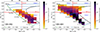 |
Fig. 4. Predicted distribution of OB stars with a NS (left panel) and BH (right panel) companion in the Hertzsprung–Russell diagram. The green line is the ZAMS, and the black line is the terminal-age main sequence (TAMS). The blue lines represent evolutionary tracks of non-rotating core hydrogen burning single stars, with the indicated initial masses. The dashed red lines show the boundaries of the three groups of stars defined in the main text, i.e. Teff = 31.6 kK, log L/L⊙ = 5, and the MS evolutionary track of a 8.9 M⊙ single star. On top, we label several spectral types at their approximate effective temperature. |
As we discuss in more detail below, the majority of the MS components below ∼15 M⊙ are expected to rotate close to critical rotation and display themselves as OBe stars. The remaining ones are also expected to rotate rapidly. As most NS-forming binaries break up due to the NS birth kick (see below), we expect many more Be stars to not have a NS companion than to be part of a NS binary.
The highest mass of a MS companion to a WD produced in our grid is ∼12 M⊙ (Fig. 6). As we do not expect newborn WDs to receive kicks like NSs, all WDs are predicted to remain in binary systems, mostly associated with fast-rotating companions, some of which may be observed as WD BeXBs (e.g. Gaudin et al. 2024; Marino et al. 2025). Since our model grid is highly incomplete for WD binaries, their detailed analysis is beyond our scope, and we focus on NS/BH-forming systems.
Since our model predicts more mergers for less massive systems, we expect more BH than NS binaries in the SMC, as is shown in the right panel of Fig. 4. We find that the MS companions of BHs are stretching over a wider mass and and temperature range. While BHs are only formed from primaries above ∼18 M⊙, our BH forming binaries can have stable mass transfer for initial mass ratios as low as 0.3 (Fig. A.1). Due to the different accretion efficiencies of Case A/B binaries (≲10% for Case B and up to ∼60% for Case A), we find the lowest mass MS companions (6 M⊙) to BHs in our models formed in Case B systems but the most massive ones (near 100 M⊙) formed in Case A systems (Fig. G.5). The difference in accretion efficiencies also leads to a stronger surface abundance enrichment for the mass gainers in Case A systems (Fig. G.8).
Towards higher masses, our results become incomplete, but pair-instability will also reduce the number of BH binaries produced there (our most massive BHs are ∼38 M⊙; see below). As the our most massive MS star models undergo envelope inflation, we expect some early B supergiants companions to BHs (cf. Quast et al. 2019). The peak of the MS companion mass distribution is near 10 M⊙, close to that of the NS companions. Most of the BH companions are expected to rotate very rapidly.
To obtain absolute numbers, we integrated the number densities for three groups of stars, mainly depending on the location of the MS component, or of the more massive star in the case of pre-interaction binaries, in the HR diagram as follows (see Fig. 4 for the group borderlines).
-
Group 1: MS stars with masses above 9 M⊙ and luminosities below 105 L⊙;
-
Group 2: MS stars with luminosities above 105 L⊙ and effective temperatures above 31.6 kK;
-
Group 3: MS stars with luminosities above 105 L⊙ and effective temperatures below 31.6 kK.
The chosen boundaries are motivated as follows. The lowest initial primary mass in our binary model grid is 5 M⊙. The most massive merger product involving 5 M⊙ primaries occur in systems with an initial mass ratio of 0.95, and produce 9.02 M⊙ merger products according to Eq. (2). We therefore chose a lower mass limit of 9 M⊙ to ensure completeness of the merger products and mass gainers. Furthermore, the lowest initial primary mass for forming BHs in our Case B system is 17.8 M⊙ (Fig. 2), whose luminosity at terminal-age main sequence is about 105 L⊙. Finally, we chose an effective temperature of 31.6 kK do distinguish between O type and B type MS stars.
The predicted numbers and fractions of the pre- and post-interaction OB stars are presented in Table 2 and Fig. 5, respectively. To obtain the proper fractions, we include the OB stars produced by the post-interaction single star channels, which are merger products and runaway stars.
Predicted numbers of the pre- and post-interaction MS OB stars in our fiducial synthetic SMC population.
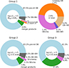 |
Fig. 5. Pie charts for the predicted numbers of pre-interaction MS OB stars primaries, and of OB stars in different types of post-interaction binaries, divided into three groups, Group 1 (top left; top right provides a zoom-in), Group 2 (lower left), and Group 3 (lower right), based on luminosities and effective temperatures. The considered types of binary stars and the corresponding fractions with respect to the total number within the considered group are indicated by text. The corresponding absolute numbers in each wedges are listed in Table 2. |
In Group 1 we find 742 O type and 2398 B type stars, of which 2746 (87.5%) reside in pre-interaction binaries, 155 (4.9%) are merger products, and 42.6 (1.4%) are runaway stars. The remaining ∼200 OB stars have evolved companions.
Group 1 contains 13.6 OB stars with NS companions, most of them B type stars, which implies that only 0.4% of the stars in this group would have a NS companion. At the same time, we expect 4.9% of the MS stars in Group 1 to orbit a BH companion, which is 149 OB+BH binaries in Group 1, 131 of them with a B star. The vast majority of them is expected to be X-ray silent (cf. Sen et al. 2024).
Group 1 is further expected to contain 30.7 OB+He-star binaries, with none of them expected to produce dense enough winds to appear as WR star. However, their winds may collide with the OBe disc or with the wind of their companion, which may turn them into observable X-ray sources (Langer et al. 2020a). We further find 3 WD binaries in Group 1, representing the high mass end of the WD companion mass distribution.
The high-mass Groups 2 and 3 contain 329 O-type stars and 65.5 B supergiants, respectively, which corresponds to 9.3% and 1.8% of all considered OB stars, which means that Group 1 contains 88.9% of them. By design, Groups 2 and 3 contain essentially no NS binaries or runaway stars. However, the most massive BHs and the WR binaries will be found in these groups. With about 10%, the fraction of OB stars with evolved companions is almost twice that in Group 1, with 21.4 (6.5%) and 3.97 (6.1%) of the MS stars forming O+BH and B+BH binaries in Groups 2 and 3, respectively. Also the MS merger fraction in Group 3 is very high with 27.6%.
These numbers are determined by several factors. The fraction of MS merger products goes up with mass due to the growth of the parameter space of Case A mergers (Appendix A). The general decreasing of merger fraction for higher primary masses leads to the increasing of the expected number of post-interaction binaries. This is also relevant for the lower number of NS star binaries compared to BH binaries, which is aggravated by the adopted NS birth kicks, and the neglect of BH kicks. Of course, a different lower mass limit or criterion for BH formation will also shift the relative numbers. The fraction of OB+He-star binaries is at just 10–20% of the OB+cc binaries, because their lifetimes are determined by their core He burning time, while the lifetimes of the former is fixed by the remaining lifetime of the OB star after the formation of the compact object, which is a fair fraction of their MS lifetime.
3.3. Number of post-interaction binaries
While the prediction of MS mergers from our grid is incomplete below ∼9 M⊙ (see above), our choice of the lowest initial primary mass of 5 M⊙ guarantees completeness for the expected NS and BH binaries. In the previous subsection, we used the 9 M⊙ limit for a meaningful comparison of the number of evolved binaries with that of MS stars. Here, we used our complete grid down to primary masses of 5 M⊙, in order to derive absolute numbers of expected post-interaction binaries in the SMC, as well as their mass dependence.
The numbers of the various types of binary systems consisting of a MS star (the mass gainer) and a post-MS companion predicted to exist in the SMC are shown in Table 3 and Fig. 6. In Table 3, we distinguish core-helium burning stripped mass donors originating from three different initial donor mass ranges, which roughly correspond to those forming WDs, NSs, and BHs, respectively, according to our assumptions (Sect. 2.5). We expect that the numbers in Table 3 and Fig. 6 are complete, except for the WDs (Mi, 1 ≤ 10 M⊙). Note, however, that while the initial mass limits for forming a certain compact object type are rather sharp for Case B binaries, the emerging helium star mass in Case A systems is not only a function of the initial donor mass but also of the initial orbital period (Wellstein et al. 2001; Schürmann et al. 2024). We can see the effect of this in Fig. 2, which shows that 17.8 M⊙ donors form BHs in Case B systems but NSs in Case A evolution (see also the plot for the initial donor mass of 10 M⊙ in Fig. A.1).
Number of post-MS companions of OB stars in our fiducial synthetic SMC population.
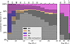 |
Fig. 6. Fractions of different types of post-MS companions of OB stars in our fiducial synthetic binary population relative to all post-MS companions, as a function of the mass of the OB star. For the companions, we distinguish core-helium burning stars (magenta), white dwarfs (blue), NSs (yellow), and BHs (grey). Shading identifies those companions that are paired with an OB star that rotates with more than 95% of its critical rotational velocities. The absolute number of binaries with post-MS companions expected in the SMC for each mass bin is given on top of the bin. The high-mass end (30–100 M⊙) is presented with a wider bin width. |
Table 3 further gives the predicted number of OB+WR binaries, and for the much smaller fraction of them in which the WR star is expected to be hydrogen-free. We also gave the small number of WR stars produced in very massive and very close binaries in our sample undergoing chemically homogeneous evolution (CHE; see below) in Table 3, for completeness. Finally, we listed the predicted number of OB stars with NS and BH companions. We also counted the number of binaries that are disrupted due to the adopted NS birth kick in Table 3, while Fig. 6 shows only the remaining binaries. Since our fiducial model ignores BH birth kicks, none of our model binaries is broken up when a BH is formed.
In Table 3 and Fig. 6, we also distinguished systems, in which the mass gainer is spun up to close-to-critical rotation and designate them as OBe stars. Notably, we find that 60–100% of the post-interaction systems contain an OBe star. Besides the high efficiency of the spin-up process, these numbers reflect the generally low mass-loss rates of our SMC MS star models, which effectively spins down star only above ∼30 M⊙.
Our overview plot for 10 M⊙ donors (Fig. A.1) shows that we expect the lowest-mass MS stars with a NS companion to have ∼6.5 M⊙. Similarly, Fig. 2 shows that the lowest mass OB+BH progenitors have initial mass ratios near ∼0.35, implying BH companion masses above ∼6.2 M⊙. Therefore, we do not expect NS or BH binaries in mass bins to the left of the 6 − 8 M⊙ bin in Fig. 6. The numbers on top of the bins in Fig. 6 show that the number of systems with MOB > 100 M⊙ that we might be missing is negligible.
As is shown in Fig. A.1, we expect Case C mass transfer (mass transfer with a core-He depleted mass donor) in a small range of initial orbital periods for initial donor masses ≲15.8 M⊙. Furthermore, about half of them may undergo stable mass transfer (Ercolino et al. 2024). We ignored those in our statistics, because they have a negligible lifetime as post-interaction binary given that they have exhausted He in their core before the mass transfer begins. Their fates are uncertain and may be quite diverse (Marchant et al. 2021; Ercolino et al. 2024).
To interpret the numbers shown in Table 3 and Fig. 6, it is helpful to consider some basic trends in our summary plots (Fig. 2 and Appendix A). For the lowest initial donor masses in our model grid (5 M⊙, Fig. A.1), binaries that can avoid merging occupy a small corner in the Case A regime and a somewhat larger triangular region in the high-mass ratio region of the Case B regime, and the models with the largest orbital periods are non-interacting systems. This shows, in agreement with many previous detailed binary evolution calculations (Pols 1994; Wellstein et al. 2001; de Mink et al. 2007), that only ∼10% of all binary systems with donor masses of 5 M⊙ are expected to survive their first mass transfer, and appear in Table 3 and Fig. 6. The other ∼90% are expected to merge4. For larger initial donor masses, the surviving fraction increases and reaches about 60% above 30 M⊙.
Our population synthesis model predicts a similar number of OB+He-star systems in the SMC formed from the initial mass ranges of NS (Mi ≃ 10–17 M⊙: 20.9) and of BH progenitors (Mi ≳ 17 M⊙: 23.1). This is so because the IMF predicts a similar number of systems in both mass ranges, and the shorter lifetime of the more massive binaries is compensated for by a smaller merger fraction. Notably, our fiducial model also predicts 6.7 WR+O star binaries. Consistent with Fig. 5, many more BH-binaries (210) than NS-binaries (24.7) are predicted to exist in the SMC, most of them with OBe type MS components.
Besides the binaries emerging from stable mass transfer, there are 0.04 O+WR and 0.32 O+BH having close orbits but not undergoing any mass transfer. These binaries are formed from tidally induced CHE (de Mink et al. 2009; Marchant et al. 2017). The primary stars are spun up by tides, and the enhanced rotational mixing prevents the establishment of the chemical gradient. Consequently, the stars evolve directly into helium stars without significant expansion. In our model grid, this process occurs with initial primary mass above 70 M⊙, initial mass ratio below 0.4, and initial orbital period around 1.6 days. This small parameter space makes the expected number of CHE products in the SMC very small (see below). In addition, CHE can also occur in massive near-equal-mass binaries, which does not produce O+BH phases but only very brief WR+BH phases (Marchant et al. 2016).
Figure 6 shows the predicted relative fractions of compact and He-star companions to OB stars as the function of mass. The total BH fraction is nearly constant at about 70%. The OBe fraction is a decreasing function of the OB stars mass. Here, most MS star companions below ∼15 M⊙ are Be stars. For higher masses, the OBe+BH fraction drops, which reflects the growing fraction of Case A systems, where stars are braked by tides. Above 40 M⊙, stars are spun down through wind braking. The NS fraction reaches a maximum near MOB = 8 M⊙ with a value about 20% and then decreases to zero near 30 M⊙. The most massive O+NS binaries form in Case A systems, which feature a strong tidal interaction and a high accretion efficiency. The He-star fraction is nearly constant with ∼20%, which is in the range inferred by El-Badry et al. (2022). A distribution of OB star masses in NS and BH binaries is provided in Fig. G.5.
3.4. Properties of OB+He/WR binary systems
Here, we first discuss the observable properties of the WR+O star binaries in our fiducial synthetic population. We compare those with the observed SMC WR stars in Sect. 5.4. The total predicted number of WR stars in the SMC is 6.7. All of them are formed through binary interaction, including tide-induced CHE, as the adopted mass-loss rate is not high enough to form WR stars through wind-stripping (see Fig. G.1 for our non-rotating single star models).
The top panel of Fig. 7 shows the predicted distribution of the WR components of OB+WR binaries in the HR-diagram, together with its 1D-projections in the top and right plots. The predicted effective temperatures of most of WR models are slightly cooler than those of pure He star models (blue line in Fig. 7). While the H-rich envelope of these donor stars gets nearly completely stripped by mass transfer, the remaining hydrogen leads to larger radii and smaller surface temperatures of stripped stars, compared to hydrogen-free models (Schootemeijer & Langer 2018; Gilkis et al. 2019; Laplace et al. 2020). In the majority of our models, the hydrogen layer is not removed by the relatively weak winds in the WR phase at this metallicity. In our synthetic population, the WR models with log Teff/K = 4.9 have a surface hydrogen mass fraction of about 0.3. Models with a surface temperatures above log Teff/K = 5.1 are hydrogen-free WR. The predicted population is sharply cut off at log L/L⊙ = 5.6 due to the threshold luminosity for defining WR stars (see Sect. 2.4). Towards the higher luminosities, the predicted number drops as a consequence of the adopted IMF.
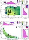 |
Fig. 7. Distributions of properties of the predicted SMC OB+WR binary population. The top panel shows the distribution of the predicted position of the WR components in the Hertzsprung Russell diagram (background colours), where the colour indicates the expected number per pixel (see colour bar on the top right). The total number of observed WR star components, or WR binaries, is four. The plots to the right and on top give the 1D-projections of the distribution, with the inset magnifying the WR binaries produced via chemical homogeneous evolution (CHE). The black circles and diamonds represent the WR components of the observed WR binaries, and single WR stars, in the SMC (Foellmi et al. 2003; Foellmi 2004; Koenigsberger et al. 2014; Hainich et al. 2015; Shenar et al. 2016, 2018), where the numbers are related to the identifier, e.g. ‘1’ for ‘SMC AB1’. The dashed blue line is the zero-age main sequence of helium star models (He-ZAMS) with SMC metallicity (Köhler et al. 2015), with the indicated helium star masses. The bottom panel shows the distribution of the predicted WR binaries in the plane of orbital period versus the orbital velocity of the WR component. Here, the black symbols represent the projected orbital velocity semi-amplitudes of the observed WR+O star binaries (circles) and of the WR+WR binary SMC AB5 (diamond). |
The bottom panel of Fig. 7 shows the distribution of the orbital periods of our OB+WR binary models, and the orbital velocities of the WR components. The orbital periods span a wide range, from ∼3 days to ∼3 years, with about half of the population below 30 days. We do not find shorter-period WR binaries because our ZAMS binaries with the shortest initial orbital periods evolve into contact and eventually merge due to L2-overflow (orange colour in Fig. A.2). The relation between the orbital velocity, υorb, WR, and orbital period, Porb, is determined by
 (10)
(10)
where MWR is the mass of WR star, and G is the gravitational constant. The corresponding orbital velocities go beyond 400 km s−1 for the short period models, and go down to ∼20 km s−1 for the longest period binaries. The orbital velocity distribution between 200 km s−1 and 350 km s−1 is rather flat because the accretion efficiency in our Case A binaries is increasing towards shorter periods, increasing the scatter in stellar masses in Eq. (10). In about two thirds of our WR binary models, the O star is more massive than the WR star (see Fig. G.3).
The insets in Fig. 7 magnify the small contributions from binary models that evolve through mass transfer and produce hydrogen-free WR stars, and those that form WR stars through CHE, which avoid mass transfer (cf. Table 3). While CHE WR stars are expected to have a hydrogen-rich phase during late hydrogen burning and early helium burning (Koenigsberger et al. 2014; Schootemeijer & Langer 2018), we did not include this short phase in our statistics (cf. Fig. G.2).
Our fiducial SMC population also contains a large number of OB+He-star binaries, in which the wind of the He-star is expected to be transparent such that WR-type emission lines would not be produced. These so-called ‘stripped star binaries’ largely lack observed counterparts (Götberg et al. 2023; Drout et al. 2023). It has been suggested that, at least the more massive of such systems, may appear as hard X-ray sources, with X-rays being produced by the collision of the He-star wind with the OBe disc and the OBe star wind (Langer et al. 2020a). While their correspondence to the sub-class of BeXBs called γ Cas-stars is debated (Nazé et al. 2022; Gunderson et al. 2025), the nature of the companion to OBe stars in observed BeXBs is often unclear. Therefore, the predicted OB+He-star binaries could contribute to the large BeXB population of the SMC. This would reduce the discrepancy between our predicted number of OBe-NS systems and the observed number of BeXBs (cf. Sects. 3.5, 5.2).
3.5. Properties of OB+NS binary systems
We find ∼25 OB+NS binaries in our fiducial synthetic population (cf. Table 3). We compare the synthetic with the observed population in Sect. 5.2 and discuss implications in Sect. 6. Figure 8 presents their orbital period distribution. We find two distinct sub-populations with orbital period peaks near 10 and 150 days, which are associated with the different modes of mass transfer. As is seen in Figs. 2 and A.1, OB+NS binaries are formed from two clearly separated triangular regions in the Case A and Case B regimes due to the upper limit on mass transfer rate set by Eq. (1). In addition, some OB+NS binaries have orbital periods exceeding the upper initial orbital period bound (≃3000 days), which are widened by the SN kicks.
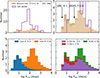 |
Fig. 8. Distributions of the orbital periods of the ∼25 OB+NS binaries in our fiducial synthetic SMC population. Upper left: Predicted period distribution (yellow histogram), where the ∼21 OB+NS binaries in which the OB stars rotates faster than 95% of their critical rotational velocity are indicated by shading (labelled ‘OBe’). The period distribution of observed BeXBs in the SMC (Haberl & Sturm 2016) is plotted as purple line. Upper right: A zoom-in of the upper left panel. The B star + radio pulsar binary J0045-7319 (Bell et al. 1995) and the supergiant X-ray binary SMC X-1 (Rawls et al. 2011; Falanga et al. 2015) are indicated by arrows. Lower left: The same predicted distribution as in the top panels, with the colours indicating which of the systems formed through Case A and Case B mass transfer (blue and orange, respectively), with the corresponding total numbers given in the legend. Lower right: The same predicted distribution as in the top panels, with the colours indicating which type of SN, and therefore which NS kick distribution, was assumed for the different systems [green for electron-capture SN; red for helium-envelope-stripped SN (CCSN-C); purple for hydrogen-envelope-stripped SN (CCSN-He); cf. Sect. 2.6]. The predicted total numbers related to different SN types are given in the legend. |
Depending on the final structure of our donor stars, we assumed that NSs are formed through different types of SNe, with correspondingly different NS birth kick distributions (cf. Sect. 2.6) are distinguished. We find ∼6.8 OB+NS binaries in which the NS was assumed to form via an electron capture SN (ECSN), 13.9 via hydrogen-stripped (CCSN-He), and 3.8 vie helium-stripped SNe (CCSN-C). ECSNe contribute a considerable fraction of the population at orbital period around 150 days, where the second dredge up of the primary star, which would reduce the helium core mass in single stars, is avoided due to the mass transfer, making ECSNe to occur much more frequently than in single stars (Podsiadlowski et al. 2004). We see that systems with a He-envelope-stripped SN prefer narrow orbits since the binary has to be close enough to get the donor star deeply stripped (also see Ercolino et al. 2025). Systems with H-envelope-stripped SNe do not show a strong orbital period preference.
Figure 9 presents the predicted distribution of eccentricities of our OB+NS binary population. It peaks at around 0.3. The OB stars of highly eccentric binaries have the chance to fill their Roche lobe during periastron passage, which causes the number of systems to drop in the high-eccentricity region. Due to the difference in the magnitude of the adopted kicks, ECSN mainly contributes binaries with e ∼ 0.3, while stripped SN contributes most of high-e binaries.
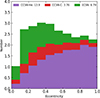 |
Fig. 9. Distribution of the eccentricities of our OB+NS model binaries, with the colours indicating which type of SN was assumed for the different systems, as in the bottom right panel of Fig. 8. |
We further show the distribution of OB+NS binaries in the orbital period-eccentricity plane in Fig. 10. We see that wide binaries tend to have higher eccentricities since they are more easily disrupted than close binaries. Further, this plot confirms the prediction of two distinct populations with orbital periods of ∼10 d and ∼150 d, which have similar eccentricity distributions. The upper left edge is populated by systems that undergo Roche lobe overflow (RLO) during periastron passage.
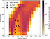 |
Fig. 10. 2D distribution of the ∼24 OB+NS binaries of our fiducial synthetic SMC population in the orbital period – eccentricity plane. The number in each pixel is colour-coded. The 7 SMC BeXBs with eccentricity measurements (Townsend et al. 2011; Coe & Kirk 2015) are indicated by black diamonds. The B star + radio pulsar binary (Kaspi et al. 1994; Bell et al. 1995) is marked by a black star, the supergiant X-ray binary SMC X-1 by a black triangle (Falanga et al. 2015). |
3.6. Properties of OB+BH binary systems
Figure 11 gives an overview of selected properties of the OB+BH binaries in our fiducial synthetic SMC population. The total number of predicted systems is ∼210, which means that ∼5% of the O and early B stars are expected to have a BH companion (Sect. 3.2). The top histogram of Fig. 11 implies that the majority of BHs are expected to have B star companions. We find ∼135 systems (64%) with a MS star mass below 15 M⊙, Those systems are predicted to contain rather light BHs (5–10 M⊙ for most, up to 20 M⊙ for ∼10%) in orbits with typically 100 d periods, in which the B star moves with 20–60 km s−1. The top histogram shows that most of these B stars are expected to be Be stars, since the corresponding stellar model rotates faster than with 95% of its critical rotation velocity.
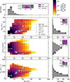 |
Fig. 11. Properties of the ∼211 OB+BH binaries in our fiducial synthetic SMC population (cf. Table 3), as function of the mass of the OB star. The three main plots show the 2D number density distributions of the systems, with the OB star mass on the X axis, and BH mass, orbital period, and OB star orbital velocity semi-amplitude on the Y axis, respectively. The number density is colour coded (see colour bar on the top right). The known OB+BH binaries, irrespective of their host galaxy metallicity, are marked by blue symbols, and correspond to MWC 656 (Casares et al. 2014), Cyg X-1 (Miller-Jones et al. 2021), LMC X-1 (Orosz et al. 2009), M33 X-7 (Ramachandran et al. 2022), VFTS 243 (Shenar et al. 2022a), and HD 130298 (Mahy et al. 2022). The BH nature of the secondary star in MWC 656 debated in the literature. The solution by Janssens et al. (2023) is labelled by ‘MWC 656 (new)’ and connected to the solution by Casares et al. (2014) through a red line. The four histograms give the corresponding 1D projections, with shading identifying rapidly rotating OB stars (labelled ‘OBe’), and insets magnifying the small contributions from chemically homogeneous evolution (CHE). The orbital velocity semi-amplitudes for observed systems are calculated using Eq. (11) with the observed masses and orbital periods. The errors are calculated by error propagation. |
The O star systems are expected to contain BHs spanning a wider mass range, with 95% of them in the range of 5–25 M⊙, and a few with BHs up to 35 M⊙. There orbital periods and orbital velocities spread a bit wider than those of the B star systems, and in particular we expect O star systems with orbital periods below 10 d, with O star orbital velocities of up to 200 km s−1. However, also many systems with wider orbits and orbital velocities well below 100 km s−1 are predicted. As in the B star regime, most O type companions are found to rotate very rapidly.
The expected number of systems drops for higher MS star masses, mostly because of the adopted IMF. Below 10 M⊙, the chance that the companion star is massive enough to form a BH decreases. Our lowest-mass MS star with a BH companion has about 6 M⊙ (cf. Fig. 6). The BH mass distribution is also affected by the IMF. The lightest BH we predict has ∼4.9 M⊙, for which the 6.6 M⊙ pre-collapse star ejected about 0.5 M⊙ of helium-rich envelope, and 1.2 M⊙ is lost due to the release of gravitational binding energy. The most massive BH in our model sample weighs about 35 M⊙, and the mass ejection from its progenitor is set by the pulsational-pair instability (PPI) mechanism (cf. Sect. 2.5).
The majority of our OB+BH binaries have orbital periods around 100 days. Binaries that are widened by the PPI-induced mass loss occupy the period regime above 3000 days. The effect of tides, which can limit the spin-up of the accreting MS star, is relevant only in the closest binaries. Therefore we expect OBe companions to BHs in most of the wide binaries ( Porb > 10 days), while slower rotators dominate in closer binaries. The most massive MS stars may rotate relatively slowly even in wide binaries because of wind braking (Langer 1998).
The models in our grid that in principle could produce the OB+BH systems with the most massive MS stars are those very massive systems that start with a mass ratio close to 1. However, at higher initial primary masses, the minimum initial mass ratio above which the secondary star ends core hydrogen burning before the primary ends its life is decreasing (Fig. A.2)5. Therefore, those systems are assumed to merge when reverse mass transfer starts, such that they do not contribute to our synthetic SMC compact object binary population. Very massive OB stars are also not produced from the most massive systems with lower mass ratios because the accretion efficiency is quite limited, and stellar wind mass loss is also considerable at the highest masses. Therefore, our population has no statistically significant contribution to the BH binary population at OB star masses above about 70 M⊙.
Comparing with the orbital period distribution of our NS binaries (Fig. 8 and G.6), we see that the clear signature of the two different modes of mass transfer is absent in the BH binary period distribution (middle panel in Fig. 11). The reason is that more binaries near the Case A/B boundary avoid merging in the BH-forming regime compared to the NS-forming regime (see Fig. A.2), which fills the orbital period gap between the two modes.
The lowest panel of Fig. 11 presents the distribution in the OB star mass – orbital velocity semi-amplitude of OB star, KOB, plane. In contrast to the WR binaries, which are assumed to be circular as consequence of the RLO, the assumed mass loss at BH formation does produce a kick, which makes the orbits mildly eccentric. Therefore, KOB is defined here by
 (11)
(11)
where Mcc is the mass of compact object. Inclination effects are not included here. The mass loss during the BH formation produces eccentricities of less than 0.1, which makes the deviation of the orbital velocities of OB stars from their semi-amplitudes within 10%. Corresponding to the peak of the orbital period distribution of about 100 days seen in the middle panel, our OB+BH binaries have velocity semi-amplitudes peaking near 40 km s−1. The highest velocity semi-amplitudes we find are about 250 km s−1 (Fig. G.6), which is near the initial orbital period boundary between stable mass transfer and L2 overflow (see Figs. 2, A.1, and A.2).
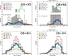 |
Fig. 12. Orbital period (left plots) and V band magnitude or mass (right) distributions of the OB+NS (top) and OB+BH (bottom) binaries resulting from our parameter variations. The predictions from the different population models are shown with differently coloured lines (see legend), where the predictions from the fiducial model are indicated by the hatched histograms with blue thick lines. The population models that produce the same distributions as the fiducial model are not shown in the corresponding plots. In the bottom plots, the SFH-R distributions are very close to the fiducial ones. We show the distributions of the observed SMC BeXBs in the upper panels with grey histograms. The observed orbital periods and V-band magnitudes of the SMC BeXBs are from Haberl & Sturm (2016). |
4. Parameter variations
Predicted populations derived with various different assumptions.
For our SMC population synthesis, we cannot change the underlying stellar evolution models. Therefore, uncertain assumptions in those, in particular concerning the efficiency of mass transfer or the criterion for unstable mass transfer and merger, cannot be varied here. However, we can vary the parameters that enter directly into the population synthesis calculations. Those are related to assumptions on compact object birth kicks, on the time dependence of the star formation rate, on the initial binary parameter distributions, on the lowest rotation velocity of OBe star, and on the upper core mass limit for NS formation. With this idea, we introduce the following population synthesis models, in which only the mentioned parameter differs from the parameters adopted in our fiducial population synthesis calculation.
-
Kick-265: the distribution of NS kick velocities was taken to be the Maxwellian distribution with σ = 265 km s−1 for all types of SNe.
-
Kick-0: All kick velocities were fixed to zero.
-
Kick-BH: BHs produced by fallback of previously ejected material may produce a SN and receive a momentum kick at birth (Janka 2012). We adopted a flat distribution in the range [0, 200] km s−1 for natal kicks imparted to newborn BHs (Kruckow et al. 2018, and Paper II);
-
logPq-flat: we used flat distributions for the initial mass ratios and logarithms of the orbital periods of our binaries.
-
SFH-S: we assumed a star formation history with no star-formation at the present time that increases up to 7 Myrs ago, before which it stays constant (see the upper panel in Fig. 13).
-
SFH-R: we assumed a star formation rate with a recent peak ∼20 − 40 Myrs ago (Rubele et al. 2015, ; see the lower panel in Fig. 13).
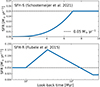
Fig. 13. Star formation history adopted to compute the population models SFH-S (upper panel, Schootemeijer et al. 2021) and SFH-R (lower panel, Rubele et al. 2015), where the dashed line indicates the constant star formation rate of 0.05 M⊙ yr−1 used in the fiducial model.
-
vcrit-0.98: the threshold value of υrot/υcrit for defining OBe stars was taken to be 0.98.
-
vcrit-0.8: the threshold value of υrot/υcrit for defining OBe stars was taken to be 0.8.
-
NS-limit: we assumed all collapsing stellar cores form NSs regardless of their helium core mass.
Below, we discuss the impact of the parameter changes on the different types of stars in the 10 simulated populations. Table 4 lists the numbers for the various types of post-interaction binaries appearing in the different model populations, as well as the number of O type stars and O type stars in pre-interaction binaries. Figure 12 compares the distributions of orbital periods and the intrinsic V-band magnitudes6 of OB stars in OB+cc binaries.
4.1. O stars
Except for Model SFH-S, our synthetic populations always contain just over 1000 O stars. Model SFH-S contains only 444, because in this model the assumed star formation rate in the SMC dropped starting 7 Myr ago. This corresponds roughly to the time spent by a 20 M⊙ model in the O star phase. In Model SFH-R, the star formation rate is equal to that in our fiducial model for the first 10 Myr, such that the number of O stars remains essentially unaffected. A similar inference holds for the number of O stars in pre-interaction binaries.
The number of O stars produced from mergers or accretion is also reduced in Model SFH-S although by a smaller factor, since they originate from smaller initial masses. We obtain somewhat more O star merger and accretion products in Model SFH-R compared to our fiducial population because the star formation rate is elevated for ages above 10 Myrs.
4.2. OBe threshold
Townsend et al. (2004) proposed that most of Be stars are very close to their critical rotation. Following this idea, we assumed in our fiducial population model that a star shows the Be phenomenon when it reaches 0.95υcrit. However, sub-critically rotating Be stars are observed (Rivinius et al. 2013, and references therein). A recent study shows that the mean rotational velocity of Be stars may be only about 0.68υcrit (Dufton et al. 2022). To assess these uncertainties in defining OBe stars, we set the threshold value of υrot/υcrit to be 0.98 and 0.80 in Models υcrit-0.98 and υcrit-0.8, respectively. This threshold value has no repercussion in the model populations other than for the count of OBe versus ordinary OB stars. However, assuming that an OBe disc is required to make an OB star appear as BeXB, the expected number of these systems is influenced.
Our results show that the effects of changing the υrot/υcrit threshold value are only considerable near the high-mass end, where wind braking becomes significant. When the υrot/υcrit threshold is increased from 0.80 to 0.98, the expected number of BH+OBe binaries is decreasing from 194 to 147, while that of predicted NS+OBe binaries changes from 23 to 20. The predicted υrot and υrot/υcrit distributions of the OB stars in OB+cc binaries are provided in Fig. G.7.
4.3. Wolf-Rayet and helium stars
Since to be counted as WR stars our stripped stars need to have luminosities above log L/L⊙ > 5.6 (Sect. 2.4), they originate from stars with initial masses above ∼40 M⊙ (cf. Fig. G.1). The lifetime of 40 M⊙ stars is only 4.5 Myr. Therefore, the number of WR+OB binaries is more than halved in Model SFR-S. It remains unaffected in Model SFR-R.
The adopted initial mass ratio and period distributions in our fiducial model prefer close binaries and high mass ratios (see Eqs. (9) and (8)) in Sect. 2.7, compared to distributions that are flat in log Pi and q. Changing to a flat distribution reduces the number of OB+He-star binaries by ∼10%. This is because the He-star population is dominated by low-mass systems (Table 3), which are formed with relatively low initial orbital periods and high initial mass ratios (Fig. A.1). Wolf-Rayet stars formed in wide binaries and low-mass-ratio binaries are boosted by a flat distribution, increasing the WR+Oe number from 4.0 (fiducial) to 5.2 (Model logPq-flat).
4.4. BH+OB binaries
We see strong changes in the number of predicted BH+OB systems when we change assumptions related to the formation of BHs. When we introduce a BH kick as described above, about 82.3 systems break up, such that their predicted number in the SMC drops by 37%, from 210 to 126 (Model Kick-BH). While this reduces the number of BH+OB binaries with orbital periods of ∼100 d, and that with B star companions (MOB ≲ 15 M⊙), the peaks of the respective distributions remain largely unchanged (Fig. 12). BH kicks produce some eccentric BH binaries with orbital periods of up to ∼40 yr. Assuming that no BHs form of course produces zero BH binaries (Model NS-limit).
In Model SFH-S, the number of BH+OB binaries is reduced from 210 (in the fiducial model) to 195 (by only 7.6%). This reflects the fact that most of our BH binaries stem from progenitors with lifetimes of more than 7 Myr (i.e. from stars below ∼40 M⊙). This is in contrast to our WR stars, which are formed from more massive primaries (Sect. 4.3). Accordingly, Model SFH-R, with a peak in star formation at an age of 30 Myr, enhances the OB+BH population by ∼100, to a total number of 313.
Also the initial binary parameter distributions affect the predicted number of OB+BH binaries. Comparing with the Sana distributions (Sana et al. 2012), a flat distribution in log P has a larger fraction of wide-orbit binaries. Hence, Model logPq-flat predicts more OB+cc binaries in period range of 100–300 days, and less below 20 days, compared to the fiducial model. The total number of BH systems in Model logPq-flat is boosted from 210 to 268.
4.5. NS+OB binaries
In our parameter study, we explore the maximum possible effects. Our Model Kick-265 shows that a Hobbs-kick applied to all NSs destroys almost all NS binaries; only 4.65 would remain in our SMC population. Assuming NSs were born without a birth momentum kick (Model Kick-0), on the other hand, increases their number by more than a factor of 4, with respect to our fiducial model. While both assumptions are not realistic, these experiments show the strong dependence of the expected numbers on the adopted kicks. Fig. 12 shows that the kicks also affect the orbital period distribution. Larger kicks shift the peak of the distribution to larger periods, while smaller kicks shift it to shorter periods.
The peak in the OB star brightness (or mass) distribution is not much affected. The upper right panel of Fig. 12 shows that the most probable OB star mass in OB+NS binaries is about 8-15 M⊙ for all different kick models, while the predicted number is largely different. In addition, different kick velocities can change the age when the OB star fills its Roche lobe during the OB+NS phase, which slightly affects the predicted total number of NS systems (NS binaries + disrupted systems).
In the fiducial model, if a star has a helium core mass MHe, c larger than 6.6 M⊙ at the core helium depletion, we assumed it to produce a BH. This expectation is based on the detailed simulation on the compactness of pre-SN stars (Sukhbold et al. 2018). In order to examine how this assumption affects our NS population, we considered the extreme case (Model NS-limit) that all stars with MHe, c exceeding 6.6 M⊙ produce NSs. While our fiducial model predicts over 200 BH systems, Model NS-limit only predicts 67 NS binaries in total, because momentum kicks are included, and because more mass is ejected by the SN than in the case of BH formation. Still, the number of NS+OB systems with orbital periods between 10 and 300 days is largely enhanced, smoothing out the bi-modality found in the fiducial model (Figs. 10 and 12). Furthermore, the number of massive and bright OB companions to NSs is increased. Their V-band magnitude can reach up to 13 mag (Fig. 12).
Finally, the number of OB+NS binaries is also affected by the adopted star formation history. There may be evidence suggesting a non-constant star formation rate in the recent past. The population of HMXBs in the SMC could infer a peak in star formation rate tens of million years ago (Antoniou et al. 2010, 2019; Ramachandran et al. 2019), which may be questionable (Schootemeijer et al. 2021, and Paper II). Rubele et al. (2015) identify two peaks at ∼30 Myrs and ∼5 Gyrs. Rubele et al. (2018) confirm the existence of the bi-modality, while the recent peak was shifted to recent 10 Myrs. On the other hand, Schootemeijer et al. (2021) find that one needs star formation rate decreases to zero within 7 Myrs to explain the dearth of young massive stars in the SMC. While Model SFH-S has little effect, the star formation history in Model SFH-R was designed to explain the large number of BeXBs found in the SMC. As is shown by the numbers in Table 4, it does its job, and boosts the predicted number of OB+NS binaries by more than a factor of 2. It affects the period and mass distributions very little.
4.6. Runaway stars
In our fiducial model, ∼74 OB runaway stars are formed, due to the disruption of the binary when the compact object forms. Table 4 shows that this number can increase substantially, depending on our assumptions. Larger NS kicks have a relatively small effect, because the NS kicks in our fiducial model already break up ∼75% of the systems. However, adding a BH kick (Model Kick-BH) roughly doubles the number, and producing only NSs and no BHs (Model NS-limit) quadruples it, and it can produce very massive runaway stars.
Notably, each of our broken-up binaries also produces a runaway NS or BH. While those BHs will likely remain undetectable, the NSs may develop into radio pulsars. We refrain here from simulating their population, because this would require us to include a significant number of new parameters, describing the radio emission, time evolution, and space motion of the pulsars (cf. Titus et al. 2020).
5. Comparisons with observations
5.1. O stars and OBe stars
Our fiducial model predicts 1072 O stars in the SMC, which include the O stars in pre- and post-interaction binaries and merger products. As is discussed in Sect. 3.1, this number may exceed the number of observed O stars, because observed counterparts of their early hydrogen-burning evolution are lacking. While a recent drop in the SFR can address this issue (Sect. 4.1), it would lead to a clear underproduction of WR stars (Sect. 5.4). A more fine-tuned SFR may fit the numbers of WR star binaries and O stars simultaneously. The observed fractions of Oe stars and of O stars with evolved companions, compared to all O stars, should be considered as upper limits when compared to our predictions, because the latter include the unobserved, potentially embedded young O stars (Schootemeijer et al. 2021).
Our fiducial population predicts that about 7% of the OB stars should appear as OBe stars. This is much less than the observed fraction (∼20%−30%, Schootemeijer et al. 2022), for which both the predicted and the empirical fractions were computed using the same V-magnitude threshold of 15.8 mag and upper limit of 13.4 mag (corresponding roughly to 9 M⊙ and 23 M⊙, respectively). Most of our post-mass-transfer binaries (> 80%) are expected to contain an OBe star (cf. Fig. 6), and it is insensitive to our adopted threshold in the fraction of critical rotation required for a model to be counted as OBe star (Sect. 4.2). While correcting for embedded stars would reduce this discrepancy, it affects mostly O stars, while the OBe population is dominated by Be stars, so this correction would be small. On the other hand, the discrepancy is smallest for the most massive OBe stars (Fig. 14). Including the O stars with masses above 23 M⊙, our fiducial model shows about 2.1% of O stars to be Oe stars, which implies 22.6 Oe stars out of 1072 O stars. The BLOeM survey has identified 20 Oe stars out of 159 O stars, giving a fraction of 13% (Shenar et al. 2024), implying about 60 Oe stars exist in the SMC with a completeness of 35%. Our parameter variations give a range for the predicted number Oe stars of 16-30 (Table 4).
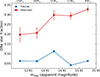 |
Fig. 14. Predicted fraction of OBe stars in our fiducial synthetic SMC population as a function of apparent Gbp magnitude (blue). The OB stars in pre-interaction binaries are included. The observed OBe star fraction is plotted with red (Schootemeijer et al. 2022). On the top we show the averaged evolutionary mass in each bin (Schootemeijer et al. 2022). |
Notably, the wind induced spin-down of rotating O stars is uncertain and could be too strong in our models (Nathaniel et al. 2025). Furthermore, it would be an effective way to boost the number of predicted OBe stars by assuming that the product of MS mergers would be rotating rapidly enough to satisfy our OBe criterion. However, as discussed in Sect. 2.2, it appears more likely that such mergers lose most of their angular momentum in the process, and appear as slow rotators after their thermal relaxation.
Our underprediction of the number of OBe stars is accompanied by a similar underprediction of the number of BeXBs (see below). To account for the large number of observed BeXBs in the SMC, a peak in the SF rate some 30 Myr ago has been proposed, which we explore in our SFH-R population model (cf. Sect. 4.5). In this scenario, also the number of predicted OBe stars is boosted by a factor of 1.7 (Table 4). While this result implies that the past SF history in the SMC may indeed play a role, its deviation from a constant SF rate would need to be more extreme to explain the high number of OBe stars within our fiducial physics assumptions.
It is therefore mandatory to consider variations in the key physics assumptions used in our binary evolution models. The most relevant ones concern the mass transfer efficiency during RLO, and the conditions applied for assuming a binary model will merge during mass transfer. A higher mass transfer efficiency would allow more IMF-preferred low-mass stars to form OBe stars, and a relaxed merger criterion would help more OB binaries to survive the first mass transfer phase and produce OBe stars. Since we cannot vary these assumptions in retrospect in our detailed binary evolution models, we discuss potential consequences qualitatively in Sect. 6. For a more quantitative discussion, we refer to Paper II.
5.2. Be X-ray binaries
There are about 150 HMXB candidates found in the SMC, of which ∼100 are identified to be BeXBs. In 63 BeXBs, the NS spin period has been measured (Haberl & Sturm 2016; Treiber et al. 2025)7. However, our fiducial model only predicts ∼25 OBe+NS binaries (Sect. 4). This discrepancy is similar to that in the number of OBe stars (see above). It may partly be remedied in a similar way.
As for the OBe stars, the SF history may play a role. In our SFH-R population model (cf. Sect. 4.5), the number of predicted BeXBs is more than doubled. Again, we conclude that a mini-starburst ∼20 Myr ago may help to reduce the discrepancy, but that other mechanisms may be worth to consider. Different to the case of the OBe stars, the number of BeXBs cannot be increased through the merger channel.
As is shown in Sect. 4.5, the number of predicted BeXBs can also be boosted by reducing the adopted NS birth kick (by up to a factor of 4.5), or the NS/BH-formation core mass threshold (by about a factor of 2 assuming our fiducial NS kicks; see Table 4). However, these factors are derived from extreme assumptions, which are unlikely to be realized in nature. NS containing BeXBs could also be produced from WD binaries through accretion-indued collapse. However, this evolutionary channel, which requires a common envelope stage and is not included in our synthetic population, works only with main sequence components in the mass range 2…4 M⊙ (Wang & Liu 2020). As such, these systems could only add a minor contribution to the low-mass end of the observed SMC BeXBs distribution (Fig. 12).
On the other hand, our model predicts about 400 OBe stars with He-star and with BH companions, which have no clear observed counterparts (see below). For both cases, the production of X-rays has been suggested (Casares et al. 2014; Langer et al. 2020a). Since the nature of the companion stars in about half of the observed BeXBs is undetermined, alternatives to assuming BHs for them could be considered (cf. Sects. 5.3 and 5.5 below). In addition, the missing of BH companions may also be explained by a different BH formation prescription that makes a large fraction of our predicted BH progenitors undergo SNe and produce NSs instead (e.g. Schneider et al. 2021; Aguilera-Dena et al. 2023).
While our fiducial model produces an insufficient number of BeXBs, their general properties agree rather well with observations. Figure 8 shows that the predicted orbital period range is similar to the observed one. While the predicted long-period tail is absent in the observed distribution, this might be so because the periods of the longest period systems are hardest to measure. Also our shortest-period systems with orbital periods below 10 days have no observed counterparts. This overprediction in the short-period regime is also found in the prediction from the POSYDON code (Rocha et al. 2024). This discrepancy could be related to tidally induced disc truncation. Short-period OB+NS binaries are less eccentric (Fig. 10), and in low-eccentricity binaries the gap between the circumstellar disc and the L1 point is so large that the NS cannot generate strong X-ray emission (Okazaki & Negueruela 2001). The observed supergiant X-ray binary SMC X-1 is close to Roche-lobe filling and has an orbital period of 3.9 days (Rawls et al. 2011; Falanga et al. 2015), which may have evolved from such short-period B(e)+NS binaries.
We also find the predicted mass distribution of the Be stars in BeXBs broadly consistent with the observed distribution (Fig. 12). We expect most OB stars in OB+NS binaries to V-magnitudes brighter than 17.5 mag (spectral types earlier than B3, or masses larger than ∼8 M⊙), which is consistent with the observed spectral types of the SMC BeXBs (McBride et al. 2008). This latest spectral type reflects the minimum mass of a MS star to have a NS companion. The observed distribution shows more stars at the high-mass end (14-15 mag), which may imply that a higher accretion efficiency is required to better reproduce the observed distribution.
We find a bi-modality in our predicted orbital period distribution, which is related to Case A and Case B binaries (Fig. 8). This bi-modality is also visible in the period-eccentricity distribution (Fig. 10). Observationally, Knigge et al. (2011) found two subpopulations of BeXBs, those in close orbits with short NS spin periods and wide orbits with long NS spin periods. We cannot compare directly to their analysis, because our model does not include the NS spin evolution. The observed bimodal feature in NS spin period distribution is suggested to relate to the underlying SN mechanisms (Knigge et al. 2011) or different accretion modes (Cheng et al. 2014; Xu & Li 2019).
As is shown in Fig. 10, observed BeXBs have eccentricity e below 0.4 (Townsend et al. 2004; Coe & Kirk 2015), while we expect half of the population to have eccentricity above that. These predicted high-e binaries also have wide orbit, making the periastron passages of NSs very fast and the corresponding systems hard to be identified as BeXBs. Recently, an extreme case of BeXBs, A0538-66, is observed in the LMC, which has one of the shortest orbital period, 16.6 d, but highest eccentricity, 0.72, of BeXBs (Rajoelimanana et al. 2017; Ducci et al. 2022), marginally covered by our predicted distribution (Fig. 10). This system may have a relatively wide pre-SN orbit, where the mass gainer was spun up by mass transfer but not affected by tides, and the SN explosion has reduced its orbital period to 16.6 d, which requires the kick velocity to have a component directed opposite to the orbital velocity of the NS progenitor.
In the SMC, one B-type star + radio pulsar binary was observed (PSR J0045-7319 Kaspi et al. 1994; Bell et al. 1995). This binary is highly eccentric with an orbital period of 51 days (Fig. 10) but it does not show X-ray emission. According to our models, it could be formed through Case A mass transfer, where tides spins down the B star, whereafter its orbit gets widened due to SN explosion.
5.3. OB+helium star binaries
Our fiducial population model predicts 235 OB+He star binaries to exist currently in the SMC, where the OB star is expected to rotate rapidly in most of them (223). With most of them in rather wide orbits (∼100 d), and the OB star rotating rapidly and dominating the optical spectra, they are difficult to identify observationally (Wellstein et al. 2001; Götberg et al. 2018). About 25 candidates have been been found recently (Drout et al. 2023), but strong biases preclude a solid comparison with our results.
Of the expected OB+He star binaries, we predict ∼32 to contain He stars more massive than ∼3 M⊙ (cf. Table 3). With luminosities exceeding ∼104 L⊙ (Langer 1989), these stars can be expected to emanate a fast wind (Vink 2017; Sander et al. 2020), which could generate X-rays through the collision with the companion star’s wind or disc. Some of the observed BeXBs in the SMC, in particular those with continuous X-ray emission, could thus contain He stars rather than NSs (Langer et al. 2020a). In fact, if the number of OB+He star binaries with massive He stars in our fiducial population would be underestimated by a similar amount as the number of OBe stars or that of BeXBs, we could expect more than 100 OB+He star binaries with He star masses above 3 M⊙. A dearth of He stars due to the delayed expansion of massive stars at low metallicity, as proposed by Hovis-Afflerbach et al. (2025) appears unlikely, as this would also make it harder to explain the large number of OBe stars in the SMC, and the drop of the observed binary fraction in evolved massive SMC stars (Patrick et al. 2025).
5.4. OB+Wolf-Rayet star binaries
There are 12 WR stars observed in the SMC, of which 4 have O star companions and 1 contains a H-deficient WR-type star (Foellmi et al. 2003; Foellmi 2004; Koenigsberger et al. 2014; Hainich et al. 2015; Shenar et al. 2016, 2018; Neugent et al. 2018; Schootemeijer & Langer 2018). From our fiducial population model, we expect 6.7 WR+O binaries in the SMC. All of the observed SMC WR star binaries have orbital periods below 20 d, where we predict 2.6 systems. Considering the Poisson error of the observed sample, our model well reproduces the observed number of WR+O binaries. While our models predict half of them to contain Oe star companions (cf. Table 4), all observed O star companions appear to be moderate rotators (projected velocities comparable or lower than ∼200 km s−1, Shenar et al. 2016, 2018). This confirms a known discrepancy between the observed rotation velocities of O stars in WR binaries and predictions from evolutionary models (Shara et al. 2020), which may suggest that circumstellar discs are easily disrupted by O star winds and radiation. Alternatively, the wind induced spin-down in the evolutionary models is underestimated (also see Nathaniel et al. 2025), or the massive accretors never spin up to critical rotation.
The location of the WR components of the WR binaries in the HR diagram are well reproduced (Fig. 7). The hydrogen-free one, the WO star SMC AB8 (Shenar et al. 2016), is covered by our H-free models with log Teff/K > 5.1 (also see Wang et al. 2019). Notably, a large temperature correction due to the optical depth of the WR wind is not expected for the SMC WR stars (Aguilera-Dena et al. 2022; Sen et al. 2023). Particularly, SMC AB7 is near the H-free region, and observationally this WR stars has the lowest surface hydrogen abundance compared to SMC AB6 and SMC AB3. The WR+WR binary SMC AB5 may have formed through the tidally induced chemically homogeneous evolution in equal-mass binaries (de Mink & Mandel 2016; Marchant et al. 2016). For SMC AB2 and AB4, their cool surface temperatures suggests that they are core-hydrogen burning (Schootemeijer & Langer 2018), core-helium-burning WR stars formed from the initial secondary stars (Pauli et al. 2023).
The agreement of the properties of the four WR+O star binaries with our models is particularly satisfying. Schootemeijer & Langer (2018) measure the slope of the H/He-gradient in the envelope, which affects their effective temperature, in a model-independent way. The result implies a H/He-gradient coincident with that left by the receding convective core during core hydrogen burning, which is indeed what we obtain in our short period binary models, which have orbital periods in the WR+O star binary phase of less than 20 d.
On the other hand, our fiducial population model predicts distributions of the binary properties of WR+O binaries that are much broader than the observed ones. Specifically, we expect 4.2 WR+O binaries with orbital periods above 20 d, while the observed ones all have shorter periods. This is reflected in the distribution of the predicted orbital velocities (bottom panel of Fig. 7). Furthermore, we expect a larger range in WR/O-mass ratios (0.5–1.5; Fig. G.3), while the three objects where this is measured show values near 0.5. Notably, both, WR+O star binaries with long orbital periods, and with less massive companions (possibly B stars) are harder to detect as such due to their orbital velocities (Fig. G.4). However extensive searches in the seven apparently single SMC WR stars have excluded the presence of companions in the long-period or large-mass-ratio part of the parameter space (Foellmi et al. 2003, Schootemeijer et al. 2024; see also Deshmukh et al. 2024 and Dsilva et al. 2020, 2022, 2023 for the Milky Way WR stars). Almeida et al. (2017) have revealed a flatter orbital period distribution in the 30 Doradus region than that assumed in our fiducial model, which would enlarge the discrepancy in the long-period regime between model predictions and observations (cf. Model logPq-flat in Sect. 4).
Even though, with 12 observed WR stars in the SMC, we have to face large statistical errors, their presence strongly disfavours the star formation history (SFH) adopted in our SFH-S-population model. As is shown in Table 4, this model produces 2.9 WR binaries, of which only 1 have an orbital period below 20 d, while four such systems are observed.
5.5. OB+BH binaries
Our fiducial model predicts 210 OB+BH binaries to reside in the SMC. While this number may appear surprisingly large at first, it is not in relation to the number of OB+NS binaries. Based on the large number of BeXBs, the order of magnitude of the OB+NS binaries in the SMC is surely at least 100. Given that, based on the Salpeter-IMF, the birthrate of NSs and BHs is comparable, differences in the number of binaries may come from differences in the lifetime of the OB companion, and from differences in the binary disruption rate. The former favours OB+NS binaries, but only slightly so, since, in our prediction, also the OB+BH binaries are dominated by B star companions (Fig. 12). Contrarily, the disruption rate strongly favours the OB+BH binaries, because 80% of the OB+NS systems are disrupted (see Table 4 for varying the kick-assumptions for BHs). Therefore, independent of strong assumptions, we may expect that the order of magnitudes of the number of OB+NS and of OB+BH binaries in the SMC are similar.
In our fiducial SMC population, we find about 1000 O stars and 40 O+BH binaries. Given that a fraction of the O stars may still be embedded (see Sect. 5.1), we would expect 4.0–6.0% of the observed SMC O stars to have a BH companion. A very similar value has been found from a comparable binary population synthesis study for the LMC (Langer et al. 2020b). So far, no massive BH binarity has been discovered in the SMC. We will therefore, when assessing the observable parameters of OB+BH binaries, compare with the known OB+BH systems found in other galaxies, wary of their metallicity difference.
Five O+BH binaries have been detected, Cyg X-1 in the Milky Way (Miller-Jones et al. 2021), LMC X-1 in the Large Magellanic Cloud (Orosz et al. 2009), M33 X-7 in the M33 (Ramachandran et al. 2022), HD 130298 in the Milky Way (Mahy et al. 2022), and VFTS 243 in the Large Magellanic Cloud (Shenar et al. 2022a). The first three sources are wind-fed X-ray binaries. The recently discovered VFTS 243 and HD 130298 are X-ray quiet and have the relatively long orbital periods (10.1 days and 14.6 days). The Be+BH nature of MWC 656 (Casares et al. 2014) is challenged by new spectral data (Rivinius et al. 2024; Janssens et al. 2023). We included both solutions in Fig. 11. While none of these systems are found at SMC metallicity, the orbital properties of the OB+BH binaries appear to be insensitive to the variation in metallicity (Fig. B.1 in Janssens et al. 2022).
Figure 11 shows that the parameters of the observed BH binaries fall into the regime that is well populated in our fiducial model, and follow the trends with the mass of the OB star. On the other hand, the orbital period distribution of our predicted OB+BH binaries peaks near 100 d, while – in particular when MWC 656 is removed – there are no observed massive BH binaries with orbital periods above 15 d. This could in part be due to an observational bias. Most massive BH binaries have so far been detected due to their X-ray emission, which is expected to be much weaker or absent in wind accreting binaries with orbital periods above ∼10 d (Sen et al. 2021, 2024). Accretion from an OBe disc might produce weak X-ray emission if the MS companion is rapidly rotating and emanates a disc (which occurs less often in the OB+WR progenitor binaries than we expect; cf. Sect. 5.4), as suggested for MWC 656. In fact, it cannot be exclude that some of the observed BeXBs in the SMC host BHs.
Optical spectroscopy, however, can be expected to detect long period OB+BH binaries. In a circular 15 M⊙ + 10 M⊙ OB+BH binary with an orbital period of 100 d, the orbital velocity of the OB star is ∼50 km s−1, which should be easily detectable even with a significant inclination of the orbit. Two long-period OB+BH candidates have been identified in the LMC, whose BH nature needs verification by follow-up observations (Shenar et al. 2022b). Still, recent and ongoing campaigns targeting the Milky Way (Mahy et al. 2022) and the SMC (Bodensteiner et al. 2025) fail to find candidate systems.
Therefore, it is possible that the predicted long-period BH binaries do not exist, or are much rarer than expected. In fact, this would be quite consistent with the apparent absence of long-period WR+OB binaries in the Magellanic clouds (see Sect. 5.4), which are progenitors of OB+BH binaries. It would be an immediate consequence of this scenario that the currently favoured channel to produce merging massive BHs, which involves a common envelope evolution of a massive star with a BH in a wide orbit (Belczynski et al. 2016), would hardly occur in nature. We will discuss implications for the mass transfer physics in massive binaries in Sect. 6.
6. Inferences for mass transfer physics
6.1. Lower mass regime
In Sect. 5, several discrepancies between our model population and the observed populations of massive stars in the SMC have been uncovered. Each of these discrepancies can potentially allow us to suggest improvements to our model assumptions, and may thus be helpful in future binary population synthesis calculations.
Our fiducial model predicts too few OBe stars above ∼9 M⊙. As the OBe star populations is dominated by the lowest mass binaries considered in our study, we may seek to change assumptions made for this mass group. Considering Fig. A.1, we see that it is a prominent feature of the lower mass binary models in our grid that the merger fraction is very high (∼80% at M1, i = 10 M⊙). A straightforward cure to obtain more OBe stars would be fewer systems merging. According to Paper II, this could about double the predicted number of OBe stars. A further increase can be achieved by increasing the mass transfer efficiency, as then more OBe stars are obtained from the more numerous lower-mass stars.
In a similar realm, one might obtain more BeXBs. However, for those, we have to match the lowest Be star mass in BeXBs. For the lowest primary mass to produce NSs of ∼10 M⊙ (Fig. A.1), the lowest Be star mass in BeXBs of ∼8 M⊙ (Fig. 12) implies that for low accretion efficiency (as in our binary models) the lowest secondary mass surviving the mass transfer event is ∼8 M⊙, and binaries with 10 M⊙ primaries and initial mass ratios below 0.8 would merge (also see Rocha et al. 2024). For fully conservative mass transfer, this critical mass ratio could be as low as 0.1.
Schürmann et al. (2024) and Zhao et al. (2024) show that the minimum mass ratio for stable mass transfer depends strongly on the mass transfer efficiency. This is not surprising, since the swelling of the secondary upon accretion is a function of its accretion rate (rather than of the mass transfer rate). Schürmann et al. (Paper II) find that this interdependence fixes the accretion efficiency to ∼50%, leading here to a critical mass ratio of about 0.5. This result is consistent with the recent study by Vinciguerra et al. (2020) based on rapid binary population synthesis of BeXBs. Schürmann et al. (Paper II) find that this can also help to explain the large number of observed OBe stars in the SMC.
While it is satisfactory to find consistent constraints on the mass transfer physics in the considered mass range (M1 ≃ 10 M⊙), the mass transfer physics itself remains not well understood. The large merger fraction and high critical mass ratio in our binary models (Fig. A.1) occur because we deemed all systems to merge, in which the energy input to achieve the required rate of mass loss from the binary exceeds the available photon energy (Sect. 2.1). The required energy input is particularly high for our models, because we assumed that the mass gainer stops accreting once it is spun up, which mostly occurs after very little accretion. Clearly, this assumption cannot hold in the binaries considered here (cf. Langer 2012). However, even with an accretion efficiency of 50%, about 3.5 M⊙ need to be removed from ∼10 M⊙ binaries. When the scenario that this matter is ejected by a photon-driven wind fails, the only other available energy source may be the orbital energy. If this is taped for ejecting the matter, we would expect significant effects on the orbital separations.
6.2. High mass regime
In the high mass regime, the main discrepancies concern not so much the number of objects – though for the OB+BH binaries it could, as none are observed in the SMC (see below). To predict as many as seven OB+WR binaries requires a low merger fraction (cf. Fig. A.2), which is only achieved with a low accretion efficiency (Schürmann et al. 2024). In this respect, out fiducial model appears acceptable.
At high mass, the main concerns are the orbital period distributions. Many massive O star binaries with orbital periods above ∼20 d are found in the LMC (Sana et al. 2013; Mahy et al. 2020) and SMC (Sana et al. 2025), which is reflected in our initial binary period distribution (Eq. 9 in Sect. 2.7). However, there are essentially no OB+WR binaries (with He-burning WR stars) found with such periods (Sect. 5.4). Similarly, even though spectroscopic searches could have identified them, there are so far not any undisputed OB+BH binaries with periods above 20 d found (Sect. 5.5). This situation is in contrast to that in the lower mass regime, where the orbital period distribution of the observed lower-mass counterparts, the OBe X-ray binaries, peaks near 100 d, in agreement with our predictions (Fig. 12). Also, the observed Be+subdwarf binaries often have orbital periods on the order of 50–200 d (Peters et al. 2008, 2013; Mourard et al. 2015; Peters et al. 2016; Wang et al. 2017, 2023).
To explain this, one might assume that long-period O star binaries merge during their mass transfer phase. The stellar type of the merger product is uncertain, and depends on the fraction of the H-rich envelope that is lost in the process. In contrast to the stars in the lower mass regime, the proximity to the Eddington limit of the high mass stars facilitates the ejection of matter from the binary system. For the same reason, however, a merger might be prevented.
Like in the lower mass regime, the physics of mass transfer is not well understood here. Possibly, the progenitors of the apparently single SMC WR stars, which are stars initially more massive than ∼35 M⊙ (Hainich et al. 2015; Schootemeijer et al. 2024), do not require a binary companion to remove their H-rich envelope (Grassitelli et al. 2021; Schootemeijer et al. 2024). However, the absence of long-period evolved massive binaries argues for some of the apparently single WR stars to be the result of a binary merger (cf. Shenar et al. 2023). While long-period WR and BH binaries are harder to detect than short-period ones (except perhaps with Gaia), the possibility that future surveys find such systems cannot be excluded. However, at this time, the chance to obtain merging double-BHs from the common envelope channel appears rather small (Sect. 5.5).
Notably, if we would assume that long-period binaries that would have produced OB+BH systems would merge, the predicted number of OB+BH binaries in the SMC would drop. The fraction depends on the mass transfer physics in the mass range 20–50 M⊙, which is not well constrained by the observed populations of post-interaction binaries. In this mass range, also the fate of massive stars is as yet unclear. While we assumed in our fiducial model that single stars in this mass range form BHs, a fraction of them may explode as SN and form NSs instead (Sect. 2.5).
7. Conclusions
Using a large grid of detailed massive binary evolution models, we have constructed a synthetic massive star population of the SMC. By comparing the number and property distributions of specific subpopulations of post-mass-transfer binaries with corresponding observed SMC populations, we were able to obtain strong constraints on uncertain model assumptions, in particular those used to describe the first mass transfer that occurs in these binaries.
To reproduce the observed OBe stars and OBe X-ray binaries, the majority of the binary stars need to avoid merging during the mass transfer. At the same time, the average mass transfer efficiency needs to be relatively high in the lower mass regime, and low in the high mass regime of the studied binaries. A lack of observed long-period (> 20 d) OB+WR binaries and possibly of OB+BH ones may imply that the observed massive long-period O star binaries merge, which would disfavour the common envelope channel for the production of merging massive BHs. The physical processes that determine the mass budget and the stability or instability of the first mass transfer remain largely undetermined.
The observed populations of evolved massive binaries are still small, in particular in the upper mass range of the investigated binaries. It is therefore desirable to enhance these samples, and thereby obtain tighter constraints, not only for the first phase of mass transfer in these systems, but also to achieve more reliable predictions of the contribution of the isolated binary channel to the observed realm of stellar explosions and gravitational wave sources.
In this formula, all digits are necessary.
Our employed initial orbital period and mass ratio distributions do not deviate strongly from flat distributions in log Pi and qi, such that the area in the summary plots are roughly representatives of the number of systems born in these areas, at the considered initial donor mass. The low-qi binaries have higher weights in population synthesis because of their longer OB+cc lifetimes.
This is expected, since the exponent α in the mass-luminosity relation for MS stars (L ∝ Mα) tends towards α = 1 for high mass (cf. Fig. 17 in Köhler et al. 2015), at which point the timescale of core hydrogen burning becomes independent of mass.
To estimate the intrinsic V-band magnitudes, We adopted the same method as in Schootemeijer et al. (2021). The distance modulus of the SMC is taken to be 18.91 (Hilditch et al. 2005), and we calculated the bolometric correction by using a polynomial fit to MIST values (Dotter 2016; Choi et al. 2016). The contribution of the Be disc in the V band was not accounted for, which is thought to be significant only in redder bands (see Fig. A.16 in Schootemeijer et al. 2022).
Online up-to-date catalogue: https://www.mpe.mpg.de/heg/SMC
While we toke 10% as the threshold value for strong tide, we also performed experiments with 30%, 50%, and 100% and the predicted OBe+cc binaries remain unchanged.
Acknowledgments
The authors thank the referee Bo Wang for the valuable feedback on the manuscript. CW is thankful for the financial support from the CSC scholarship. TS acknowledges support from the Israel Science Foundation (ISF) under grant number 0603225041 and from the European Research Council (ERC) under the European Union’s Horizon 2020 research and innovation programme (grant agreement 101164755/METAL). PM acknowledges support from the FWO senior fellowship number 12ZY523N.
References
- Abbott, B. P., Abbott, R., Abbott, T. D., et al. 2016, Phys. Rev. Lett., 116 [Google Scholar]
- Abbott, R., Abbott, T. D., Acernese, F., et al. 2023, Phys. Rev. X, 13 [Google Scholar]
- Aguilera-Dena, D. R., Langer, N., Antoniadis, J., et al. 2022, A&A, 661, A60 [NASA ADS] [CrossRef] [EDP Sciences] [Google Scholar]
- Aguilera-Dena, D. R., Müller, B., Antoniadis, J., et al. 2023, A&A, 671, A134 [NASA ADS] [CrossRef] [EDP Sciences] [Google Scholar]
- Almeida, L. A., Sana, H., Taylor, W., et al. 2017, A&A, 598, A84 [NASA ADS] [CrossRef] [EDP Sciences] [Google Scholar]
- Antoniou, V., Zezas, A., Drake, J. J., et al. 2019, ApJ, 887, 20 [NASA ADS] [CrossRef] [Google Scholar]
- Antoniou, V., Zezas, A., Hatzidimitriou, D., & Kalogera, V. 2010, ApJ, 716, L140 [NASA ADS] [CrossRef] [Google Scholar]
- Belczynski, K., Kalogera, V., Rasio, F. A., et al. 2008, ApJS, 174, 223 [Google Scholar]
- Belczynski, K., Holz, D. E., Bulik, T., & O’Shaughnessy, R. 2016, Nature, 534, 512 [NASA ADS] [CrossRef] [Google Scholar]
- Bell, J. F., Bessell, M. S., Stappers, B. W., Bailes, M., & Kaspi, V. M. 1995, ApJ, 447, L117 [NASA ADS] [CrossRef] [Google Scholar]
- Blaauw, A. 1961, Bull. Astron. Inst. Netherlands, 15, 265 [NASA ADS] [Google Scholar]
- Bodensteiner, J., Shenar, T., & Sana, H. 2020, A&A, 641, A42 [NASA ADS] [CrossRef] [EDP Sciences] [Google Scholar]
- Bodensteiner, J., Shenar, T., Sana, H., et al. 2025, A&A, 698, A38 [NASA ADS] [CrossRef] [EDP Sciences] [Google Scholar]
- Böhm-Vitense, E. 1958, Zap, 46, 108 [Google Scholar]
- Bonanos, A. Z., Lennon, D. J., Köhlinger, F., et al. 2010, AJ, 140, 416 [NASA ADS] [CrossRef] [Google Scholar]
- Brott, I., de Mink, S. E., Cantiello, M., et al. 2011, A&A, 530, A115 [NASA ADS] [CrossRef] [EDP Sciences] [Google Scholar]
- Brown, A. G. A., Vallenari, A., Prusti, T., et al. 2018, A&A, 616, A1 [NASA ADS] [CrossRef] [EDP Sciences] [Google Scholar]
- Cantiello, M., & Langer, N. 2010, A&A, 521, A9 [NASA ADS] [CrossRef] [EDP Sciences] [Google Scholar]
- Carli, E., Levin, L., Stappers, B. W., et al. 2024, MNRAS, 531, 2835 [Google Scholar]
- Carniani, S., Hainline, K., D’Eugenio, F., et al. 2024, Nature, 633, 318 [CrossRef] [Google Scholar]
- Casares, J., Negueruela, I., Ribó, M., et al. 2014, Nature, 505, 378 [Google Scholar]
- Castro, N., Oey, M. S., Fossati, L., & Langer, N. 2018, ApJ, 868, 57 [NASA ADS] [CrossRef] [Google Scholar]
- Chatzopoulos, E., & Wheeler, J. C. 2012, ApJ, 748, 42 [NASA ADS] [CrossRef] [Google Scholar]
- Cheng, Z. Q., Shao, Y., & Li, X. D. 2014, ApJ, 786, 128 [NASA ADS] [CrossRef] [Google Scholar]
- Choi, J., Dotter, A., Conroy, C., et al. 2016, ApJ, 823, 102 [Google Scholar]
- Coe, M. J., & Kirk, J. 2015, MNRAS, 452, 969 [NASA ADS] [CrossRef] [Google Scholar]
- Coleiro, A., & Chaty, S. 2013, ApJ, 764, 185 [NASA ADS] [CrossRef] [Google Scholar]
- Davies, B., Kudritzki, R.-P., Gazak, Z., et al. 2015, ApJ, 806, 21 [NASA ADS] [CrossRef] [Google Scholar]
- de Burgos, A., Keszthelyi, Z., Simón-Díaz, S., & Urbaneja, M. A. 2024, A&A, 687, L16 [NASA ADS] [CrossRef] [EDP Sciences] [Google Scholar]
- de Grijs, R., & Bono, G. 2015, AJ, 149, 179 [Google Scholar]
- de Mink, S. E., Cantiello, M., Langer, N., et al. 2009, A&A, 497, 243 [NASA ADS] [CrossRef] [EDP Sciences] [Google Scholar]
- de Mink, S. E., & Mandel, I. 2016, MNRAS, 460, 3545 [NASA ADS] [CrossRef] [Google Scholar]
- de Mink, S. E., Pols, O. R., & Hilditch, R. W. 2007, A&A, 467, 1181 [NASA ADS] [CrossRef] [EDP Sciences] [Google Scholar]
- Deshmukh, K., Sana, H., Mérand, A., et al. 2024, A&A, 692, A109 [NASA ADS] [CrossRef] [EDP Sciences] [Google Scholar]
- Detmers, R. G., Langer, N., Podsiadlowski, P., & Izzard, R. G. 2008, A&A, 484, 831 [NASA ADS] [CrossRef] [EDP Sciences] [Google Scholar]
- Doherty, C. L., Gil-Pons, P., Siess, L., Lattanzio, J. C., & Lau, H. H. B. 2015, MNRAS, 446, 2599 [Google Scholar]
- Dotter, A. 2016, ApJS, 222, 8 [Google Scholar]
- Drout, M. R., Götberg, Y., Ludwig, B. A., et al. 2023, Science, 382, 1287 [NASA ADS] [CrossRef] [Google Scholar]
- Dsilva, K., Shenar, T., Sana, H., & Marchant, P. 2020, A&A, 641, A26 [NASA ADS] [CrossRef] [EDP Sciences] [Google Scholar]
- Dsilva, K., Shenar, T., Sana, H., & Marchant, P. 2022, A&A, 664, A93 [NASA ADS] [CrossRef] [EDP Sciences] [Google Scholar]
- Dsilva, K., Shenar, T., Sana, H., & Marchant, P. 2023, A&A, 674, A88 [NASA ADS] [CrossRef] [EDP Sciences] [Google Scholar]
- Ducci, L., Mereghetti, S., Santangelo, A., et al. 2022, A&A, 661, A22 [NASA ADS] [CrossRef] [EDP Sciences] [Google Scholar]
- Dufton, P. L., Lennon, D. J., Villaseñor, J. I., et al. 2022, MNRAS, 512, 3331 [NASA ADS] [CrossRef] [Google Scholar]
- Eddington, A. S. 1929, MNRAS, 90, 54 [Google Scholar]
- Eggleton, P. P. 1983, ApJ, 268, 368 [Google Scholar]
- El-Badry, K., Conroy, C., Quataert, E., et al. 2022, MNRAS, 516, 3602 [NASA ADS] [CrossRef] [Google Scholar]
- El Mellah, I., Bolte, J., Decin, L., Homan, W., & Keppens, R. 2020, A&A, 637, A91 [NASA ADS] [CrossRef] [EDP Sciences] [Google Scholar]
- Eldridge, J. J., & Stanway, E. R. 2022, ARA&A, 60, 455 [NASA ADS] [CrossRef] [Google Scholar]
- Endal, A. S., & Sofia, S. 1978, ApJ, 220, 279 [NASA ADS] [CrossRef] [Google Scholar]
- Ercolino, A., Jin, H., Langer, N., & Dessart, L. 2024, A&A, 685, A58 [NASA ADS] [CrossRef] [EDP Sciences] [Google Scholar]
- Ercolino, A., Jin, H., Langer, N., & Dessart, L. 2025, A&A, 696, A103 [NASA ADS] [CrossRef] [EDP Sciences] [Google Scholar]
- Falanga, M., Bozzo, E., Lutovinov, A., et al. 2015, A&A, 577, A130 [NASA ADS] [CrossRef] [EDP Sciences] [Google Scholar]
- Farag, E., Renzo, M., Farmer, R., Chidester, M. T., & Timmes, F. X. 2022, ApJ, 937, 112 [NASA ADS] [CrossRef] [Google Scholar]
- Farmer, R., Renzo, M., de Mink, S. E., Fishbach, M., & Justham, S. 2020, ApJ, 902, L36 [CrossRef] [Google Scholar]
- Fichtner, Y. A., Grassitelli, L., Romano-Díaz, E., & Porciani, C. 2022, MNRAS, 512, 4573 [NASA ADS] [CrossRef] [Google Scholar]
- Foellmi, C. 2004, A&A, 416, 291 [NASA ADS] [CrossRef] [EDP Sciences] [Google Scholar]
- Foellmi, C., Moffat, A. F. J., & Guerrero, M. A. 2003, MNRAS, 338, 360 [NASA ADS] [CrossRef] [Google Scholar]
- Fortin, F., García, F., Chaty, S., Chassande-Mottin, E., & Simaz Bunzel, A. 2022, A&A, 665, A31 [NASA ADS] [CrossRef] [EDP Sciences] [Google Scholar]
- Fricke, K. 1968, Zap, 68, 317 [Google Scholar]
- Fryer, C. L., Belczynski, K., Wiktorowicz, G., et al. 2012, ApJ, 749, 91 [Google Scholar]
- Gaudin, T. M., Coe, M. J., Kennea, J. A., et al. 2024, MNRAS, 534, 1937 [Google Scholar]
- Ge, H., Webbink, R. F., & Han, Z. 2020, ApJS, 249, 9 [NASA ADS] [CrossRef] [Google Scholar]
- Gilkis, A., Vink, J. S., Eldridge, J. J., & Tout, C. A. 2019, MNRAS, 486, 4451 [CrossRef] [Google Scholar]
- Glebbeek, E., Gaburov, E., Portegies Zwart, S., & Pols, O. R. 2013, MNRAS, 434, 3497 [NASA ADS] [CrossRef] [Google Scholar]
- Golden-Marx, J. B., Oey, M. S., Lamb, J. B., Graus, A. S., & White, A. S. 2016, ApJ, 819, 55 [NASA ADS] [CrossRef] [Google Scholar]
- Goldreich, P., & Schubert, G. 1967, ApJ, 150, 571 [Google Scholar]
- Górski, M., Zgirski, B., Pietrzyński, G., et al. 2020, ApJ, 889, 179 [Google Scholar]
- Götberg, Y., de Mink, S. E., Groh, J. H., et al. 2018, A&A, 615, A78 [NASA ADS] [CrossRef] [EDP Sciences] [Google Scholar]
- Götberg, Y., de Mink, S. E., Groh, J. H., Leitherer, C., & Norman, C. 2019, A&A, 629, A134 [NASA ADS] [CrossRef] [EDP Sciences] [Google Scholar]
- Götberg, Y., Drout, M. R., Ji, A. P., et al. 2023, ApJ, 959, 125 [CrossRef] [Google Scholar]
- Grassitelli, L., Langer, N., Mackey, J., et al. 2021, A&A, 647, A99 [NASA ADS] [CrossRef] [EDP Sciences] [Google Scholar]
- Gräfener, G., Owocki, S. P., Grassitelli, L., & Langer, N. 2017, A&A, 608, A34 [NASA ADS] [CrossRef] [EDP Sciences] [Google Scholar]
- Gunderson, S. J., Huenemoerder, D. P., Torrejón, J. M., et al. 2025, ApJ, 978, 105 [Google Scholar]
- Guo, Y.-L., Wang, B., Chen, W.-C., et al. 2024, MNRAS, 530, 4461 [Google Scholar]
- Haberl, F., & Sturm, R. 2016, A&A, 586, A81 [NASA ADS] [CrossRef] [EDP Sciences] [Google Scholar]
- Hagen, L. M. Z., Siegel, M. H., Hoversten, E. A., et al. 2017, MNRAS, 466, 4540 [NASA ADS] [Google Scholar]
- Hainich, R., Pasemann, D., Todt, H., et al. 2015, A&A, 581, A21 [NASA ADS] [CrossRef] [EDP Sciences] [Google Scholar]
- Hamann, W. R., Koesterke, L., & Wessolowski, U. 1995, A&A, 299, 151 [Google Scholar]
- Harris, J., & Zaritsky, D. 2004, AJ, 127, 1531 [NASA ADS] [CrossRef] [Google Scholar]
- Hastings, B., Wang, C., & Langer, N. 2020, A&A, 633, A165 [NASA ADS] [CrossRef] [EDP Sciences] [Google Scholar]
- Hastings, B., Langer, N., & Puls, J. 2023, A&A, 672, A60 [NASA ADS] [CrossRef] [EDP Sciences] [Google Scholar]
- Heger, A., & Langer, N. 2000, ApJ, 544, 1016 [CrossRef] [Google Scholar]
- Heger, A., & Woosley, S. E. 2002, ApJ, 567, 532 [Google Scholar]
- Helton, J. M., Rieke, G. H., Alberts, S., et al. 2025, Nat. Astron., 9, 729 [Google Scholar]
- Hilditch, R. W., Howarth, I. D., & Harries, T. J. 2005, MNRAS, 357, 304 [NASA ADS] [CrossRef] [Google Scholar]
- Hill, V., Andrievsky, S., & Spite, M. 1995, A&A, 293, 347 [NASA ADS] [Google Scholar]
- Hills, J. G. 1983, ApJ, 267, 322 [NASA ADS] [CrossRef] [Google Scholar]
- Hirai, R., & Mandel, I. 2021, PASA, 38 [Google Scholar]
- Hobbs, G., Lorimer, D. R., Lyne, A. G., & Kramer, M. 2005, MNRAS, 360, 974 [Google Scholar]
- Hovis-Afflerbach, B., Götberg, Y., Schootemeijer, A., et al. 2025, A&A, 697, A239 [NASA ADS] [CrossRef] [EDP Sciences] [Google Scholar]
- Huang, W., Gies, D. R., & McSwain, M. V. 2010, ApJ, 722, 605 [Google Scholar]
- Hurley, J. R., Tout, C. A., & Pols, O. R. 2002, MNRAS, 329, 897 [Google Scholar]
- Hut, P. 1981, A&A, 99, 126 [NASA ADS] [Google Scholar]
- Igoshev, A. P. 2020, MNRAS, 494, 3663 [NASA ADS] [CrossRef] [Google Scholar]
- Janka, H.-T. 2017, ApJ, 837, 84 [Google Scholar]
- Janka, H.-T. 2012, Ann. Rev. Nucl. Part. Sci., 62, 407 [Google Scholar]
- Janssens, S., Shenar, T., Sana, H., et al. 2022, A&A, 658, A129 [NASA ADS] [CrossRef] [EDP Sciences] [Google Scholar]
- Janssens, S., Shenar, T., Degenaar, N., et al. 2023, A&A, 677, L9 [NASA ADS] [CrossRef] [EDP Sciences] [Google Scholar]
- Kaspi, V. M., Johnston, S., Bell, J. F., et al. 1994, ApJ, 423, L43 [Google Scholar]
- Kippenhahn, R., & Weigert, A. 1967, Zap, 65, 251 [Google Scholar]
- Klencki, J., Podsiadlowski, P., Langer, N., et al. 2025, A&A, submitted, [arXiv:2505.08860] [Google Scholar]
- Knigge, C., Coe, M. J., & Podsiadlowski, P. 2011, Nature, 479, 372 [NASA ADS] [CrossRef] [Google Scholar]
- Koenigsberger, G., Morrell, N., Hillier, D. J., et al. 2014, AJ, 148, 62 [Google Scholar]
- Köhler, K., Langer, N., de Koter, A., et al. 2015, A&A, 573, A71 [NASA ADS] [CrossRef] [EDP Sciences] [Google Scholar]
- Korn, A. J., Becker, S. R., Gummersbach, C. A., & Wolf, B. 2000, A&A, 353, 655 [NASA ADS] [Google Scholar]
- Kroupa, P. 2001, MNRAS, 322, 231 [NASA ADS] [CrossRef] [Google Scholar]
- Kruckow, M. U., Tauris, T. M., Langer, N., Kramer, M., & Izzard, R. G. 2018, MNRAS, 481, 1908 [CrossRef] [Google Scholar]
- Lamb, J. B., Oey, M. S., Segura-Cox, D. M., et al. 2016, ApJ, 817, 113 [NASA ADS] [CrossRef] [Google Scholar]
- Langer, N. 1989, A&A, 210, 93 [NASA ADS] [Google Scholar]
- Langer, N. 1991, A&A, 252, 669 [NASA ADS] [Google Scholar]
- Langer, N. 1998, A&A, 329, 551 [NASA ADS] [Google Scholar]
- Langer, N. 2012, ARA&A, 50, 107 [CrossRef] [Google Scholar]
- Langer, N., & Norman, C. A. 2006, ApJ, 638, L63 [Google Scholar]
- Langer, N., Fricke, K. J., & Sugimoto, D. 1983, A&A, 126, 207 [NASA ADS] [Google Scholar]
- Langer, N., Norman, C. A., de Koter, A., et al. 2007, A&A, 475, L19 [NASA ADS] [CrossRef] [EDP Sciences] [Google Scholar]
- Langer, N., Baade, D., Bodensteiner, J., et al. 2020a, A&A, 633, A40 [NASA ADS] [CrossRef] [EDP Sciences] [Google Scholar]
- Langer, N., Schürmann, C., Stoll, K., et al. 2020b, A&A, 638, A39 [NASA ADS] [CrossRef] [EDP Sciences] [Google Scholar]
- Laplace, E., Götberg, Y., de Mink, S. E., Justham, S., & Farmer, R. 2020, A&A, 637, A6 [NASA ADS] [CrossRef] [EDP Sciences] [Google Scholar]
- Ma, X., Hopkins, P. F., Kasen, D., et al. 2016, MNRAS, 459, 3614 [Google Scholar]
- Maeder, A. 1997, A&A, 321, 134 [NASA ADS] [Google Scholar]
- Mahy, L., Sana, H., Abdul-Masih, M., et al. 2020, A&A, 634, A118 [NASA ADS] [CrossRef] [EDP Sciences] [Google Scholar]
- Mahy, L., Sana, H., Shenar, T., et al. 2022, A&A, 664, A159 [NASA ADS] [CrossRef] [EDP Sciences] [Google Scholar]
- Mapelli, M. 2020, Front. Astron. Space Sci., 7, 38 [NASA ADS] [CrossRef] [Google Scholar]
- Mandel, I., & Broekgaarden, F. S. 2022, Liv. Rev. Relat., 25, 1 [Google Scholar]
- Mandel, I., & Müller, B. 2020, MNRAS, 499, 3214 [NASA ADS] [CrossRef] [Google Scholar]
- Marchant, P. 2017, Ph.D. Thesis, https://astro.uni-bonn.de/ nlanger/thesis/pablo.tif [Google Scholar]
- Marchant, P., Langer, N., Podsiadlowski, P., Tauris, T. M., & Moriya, T. J. 2016, A&A, 588, A50 [NASA ADS] [CrossRef] [EDP Sciences] [Google Scholar]
- Marchant, P., Langer, N., Podsiadlowski, P., et al. 2017, A&A, 604, A55 [NASA ADS] [CrossRef] [EDP Sciences] [Google Scholar]
- Marchant, P., Renzo, M., Farmer, R., et al. 2019, ApJ, 882, 36 [Google Scholar]
- Marchant, P., Pappas, K. M. W., Gallegos-Garcia, M., et al. 2021, A&A, 650, A107 [NASA ADS] [CrossRef] [EDP Sciences] [Google Scholar]
- Marino, A., Yang, H. N., Coti Zelati, F., et al. 2025, ApJ, 980, L36 [Google Scholar]
- McBride, V. A., Coe, M. J., Negueruela, I., Schurch, M. P. E., & McGowan, K. E. 2008, MNRAS, 388, 1198 [NASA ADS] [CrossRef] [Google Scholar]
- Menon, A., Langer, N., de Mink, S. E., et al. 2021, MNRAS, 507, 5013 [NASA ADS] [CrossRef] [Google Scholar]
- Miller-Jones, J. C. A., Bahramian, A., Orosz, J. A., et al. 2021, Science, 371, 1046 [Google Scholar]
- Mirabel, I. F. 2017, in New Frontiers in Black Hole Astrophysics, ed. A. Gomboc, IAU Symp., 324, 303 [NASA ADS] [Google Scholar]
- Mokiem, M. R., de Koter, A., Vink, J. S., et al. 2007, A&A, 473, 603 [NASA ADS] [CrossRef] [EDP Sciences] [Google Scholar]
- Mourard, D., Monnier, J. D., Meilland, A., et al. 2015, A&A, 577, A51 [NASA ADS] [CrossRef] [EDP Sciences] [Google Scholar]
- Nagarajan, P., & El-Badry, K. 2025, PASP, 137 [Google Scholar]
- Nathaniel, K., Langer, N., Simón-Díaz, S., et al. 2025, A&A, 702, 13 [Google Scholar]
- Nazé, Y., Rauw, G., Smith, M. A., & Motch, C. 2022, MNRAS, 516, 3366 [CrossRef] [Google Scholar]
- Neugent, K. F., Massey, P., & Morrell, N. 2018, ApJ, 863, 181 [NASA ADS] [CrossRef] [Google Scholar]
- Nieuwenhuijzen, H., & de Jager, C. 1990, A&A, 231, 134 [NASA ADS] [Google Scholar]
- Nomoto, K. 1984, ApJ, 277, 791 [NASA ADS] [CrossRef] [Google Scholar]
- O’Connor, E., & Ott, C. D. 2011, ApJ, 730, 70 [Google Scholar]
- O’Doherty, T. N., Bahramian, A., Miller-Jones, J. C. A., et al. 2023, MNRAS, 521, 2504 [CrossRef] [Google Scholar]
- Okazaki, A. T., & Negueruela, I. 2001, A&A, 377, 161 [NASA ADS] [CrossRef] [EDP Sciences] [Google Scholar]
- Orosz, J. A., Steeghs, D., McClintock, J. E., et al. 2009, ApJ, 697, 573 [NASA ADS] [CrossRef] [Google Scholar]
- Orosz, J. A., McClintock, J. E., Aufdenberg, J. P., et al. 2011, ApJ, 742, 84 [NASA ADS] [CrossRef] [Google Scholar]
- Packet, W. 1981, A&A, 102, 17 [NASA ADS] [Google Scholar]
- Patrick, L. R., Lennon, D. J., Najarro, F., et al. 2025, A&A, 698, A39 [NASA ADS] [CrossRef] [EDP Sciences] [Google Scholar]
- Patton, R. A., & Sukhbold, T. 2020, MNRAS, 499, 2803 [NASA ADS] [CrossRef] [Google Scholar]
- Pauli, D., Oskinova, L. M., Hamann, W. R., et al. 2023, A&A, 673, A40 [NASA ADS] [CrossRef] [EDP Sciences] [Google Scholar]
- Paxton, B., Bildsten, L., Dotter, A., et al. 2011, ApJS, 192, 3 [Google Scholar]
- Paxton, B., Cantiello, M., Arras, P., et al. 2013, ApJS, 208, 4 [Google Scholar]
- Paxton, B., Marchant, P., Schwab, J., et al. 2015, ApJS, 220, 15 [Google Scholar]
- Peters, G. J., Gies, D. R., Grundstrom, E. D., & McSwain, M. V. 2008, ApJ, 686, 1280 [Google Scholar]
- Peters, G. J., Pewett, T. D., Gies, D. R., Touhami, Y. N., & Grundstrom, E. D. 2013, ApJ, 765, 2 [Google Scholar]
- Peters, G. J., Wang, L., Gies, D. R., & Grundstrom, E. D. 2016, ApJ, 828, 47 [Google Scholar]
- Petrovic, J., Langer, N., & van der Hucht, K. A. 2005, A&A, 435, 1013 [NASA ADS] [CrossRef] [EDP Sciences] [Google Scholar]
- Pfahl, E., Rappaport, S., Podsiadlowski, P., & Spruit, H. 2002, ApJ, 574, 364 [Google Scholar]
- Podsiadlowski, P., Langer, N., Poelarends, A. J. T., et al. 2004, ApJ, 612, 1044 [NASA ADS] [CrossRef] [Google Scholar]
- Poelarends, A. J. T., Herwig, F., Langer, N., & Heger, A., 2008, ApJ, 675, 614 [Google Scholar]
- Poelarends, A. J. T., Wurtz, S., Tarka, J., Cole Adams, L., & Hills, S. T. 2017, ApJ, 850, 197 [NASA ADS] [CrossRef] [Google Scholar]
- Pols, O. R. 1994, A&A, 290, 119 [Google Scholar]
- Quast, M., Langer, N., & Tauris, T. M. 2019, A&A, 628, A19 [NASA ADS] [CrossRef] [EDP Sciences] [Google Scholar]
- Rajoelimanana, A. F., Charles, P. A., Meintjes, P. J., et al. 2017, MNRAS, 464, 4133 [NASA ADS] [CrossRef] [Google Scholar]
- Ramachandran, V., Hamann, W. R., Oskinova, L. M., et al. 2019, A&A, 625, A104 [NASA ADS] [CrossRef] [EDP Sciences] [Google Scholar]
- Ramachandran, V., Oskinova, L. M., Hamann, W. R., et al. 2022, A&A, 667, A77 [NASA ADS] [CrossRef] [EDP Sciences] [Google Scholar]
- Rawls, M. L., Orosz, J. A., McClintock, J. E., et al. 2011, ApJ, 730, 25 [NASA ADS] [CrossRef] [Google Scholar]
- Reig, P. 2011, Ap&SS, 332, 1 [Google Scholar]
- Repetto, S., & Nelemans, G. 2015, MNRAS, 453, 3341 [Google Scholar]
- Rivinius, T., Carciofi, A. C., & Martayan, C. 2013, A&ARv, 21, 69 [Google Scholar]
- Rivinius, T., Klement, R., Chojnowski, S. D., et al. 2024, in Massive Stars Near and Far, eds. J. Mackey, J. S. Vink, & N. St-Louis, IAU Symp., 361, 332 [Google Scholar]
- Rocha, K. A., Kalogera, V., Doctor, Z., et al. 2024, ApJ, 971, 133 [Google Scholar]
- Rubele, S., Girardi, L., Kerber, L., et al. 2015, MNRAS, 449, 639 [NASA ADS] [CrossRef] [Google Scholar]
- Rubele, S., Pastorelli, G., Girardi, L., et al. 2018, MNRAS, 478, 5017 [NASA ADS] [CrossRef] [Google Scholar]
- Rubio, A. C., Carciofi, A. C., Bjorkman, J. E., et al. 2025, A&A, 698, A309 [NASA ADS] [CrossRef] [EDP Sciences] [Google Scholar]
- Sana, H., de Mink, S. E., de Koter, A., et al. 2012, Science, 337, 444 [Google Scholar]
- Sana, H., de Koter, A., de Mink, S. E., et al. 2013, A&A, 550, A107 [NASA ADS] [CrossRef] [EDP Sciences] [Google Scholar]
- Sana, H., Shenar, T., Bodensteiner, J., et al. 2025, Nat. Astron., in press [Google Scholar]
- Sander, A. A. C., Vink, J. S., & Hamann, W. R. 2020, MNRAS, 491, 4406 [Google Scholar]
- Sanyal, D., Grassitelli, L., Langer, N., & Bestenlehner, J. M. 2015, A&A, 580, A20 [NASA ADS] [CrossRef] [EDP Sciences] [Google Scholar]
- Sanyal, D., Langer, N., Szécsi, D., -C Yoon, S., & Grassitelli, L. 2017, A&A, 597, A71 [NASA ADS] [CrossRef] [EDP Sciences] [Google Scholar]
- Schneider, F. R. N., Podsiadlowski, P., Langer, N., Castro, N., & Fossati, L. 2016, MNRAS, 457, 2355 [Google Scholar]
- Schneider, F. R. N., Ohlmann, S. T., Podsiadlowski, P., et al. 2019, Nature, 574, 211 [Google Scholar]
- Schneider, F. R. N., Podsiadlowski, P., & Müller, B. 2021, A&A, 645, A5 [NASA ADS] [CrossRef] [EDP Sciences] [Google Scholar]
- Schneider, F. R. N., Podsiadlowski, P., & Laplace, E. 2023, ApJ, 950, L9 [NASA ADS] [CrossRef] [Google Scholar]
- Schootemeijer, A., & Langer, N. 2018, A&A, 611, A75 [NASA ADS] [CrossRef] [EDP Sciences] [Google Scholar]
- Schootemeijer, A., Langer, N., Grin, N. J., & Wang, C. 2019, A&A, 625, A132 [NASA ADS] [CrossRef] [EDP Sciences] [Google Scholar]
- Schootemeijer, A., Langer, N., Lennon, D., et al. 2021, A&A, 646, A106 [NASA ADS] [CrossRef] [EDP Sciences] [Google Scholar]
- Schootemeijer, A., Lennon, D. J., Garcia, M., et al. 2022, A&A, 667, A100 [NASA ADS] [CrossRef] [EDP Sciences] [Google Scholar]
- Schootemeijer, A., Shenar, T., Langer, N., et al. 2024, A&A, 689, A157 [NASA ADS] [CrossRef] [EDP Sciences] [Google Scholar]
- Schürmann, C., & Langer, N. 2024, A&A, 691, A174 [NASA ADS] [CrossRef] [EDP Sciences] [Google Scholar]
- Schürmann, C., Langer, N., Kramer, J. A., et al. 2024, A&A, 690, A282 [NASA ADS] [CrossRef] [EDP Sciences] [Google Scholar]
- Schürmann, C., Xu, X. T., Langer, N., et al. 2025, A&A, 704, A219 [NASA ADS] [CrossRef] [EDP Sciences] [Google Scholar]
- Sciarini, L., Ekström, S., Eggenberger, P., et al. 2024, A&A, 681, L1 [NASA ADS] [CrossRef] [EDP Sciences] [Google Scholar]
- Sen, K., Xu, X. T., Langer, N., et al. 2021, A&A, 652, A138 [NASA ADS] [CrossRef] [EDP Sciences] [Google Scholar]
- Sen, K., Langer, N., Marchant, P., et al. 2022, A&A, 659, A98 [NASA ADS] [CrossRef] [EDP Sciences] [Google Scholar]
- Sen, K., Langer, N., Pauli, D., et al. 2023, A&A, 672, A198 [NASA ADS] [CrossRef] [EDP Sciences] [Google Scholar]
- Sen, K., El Mellah, I., Langer, N., et al. 2024, A&A, 690, A256 [NASA ADS] [CrossRef] [EDP Sciences] [Google Scholar]
- Sepinsky, J. F., Willems, B., Kalogera, V., & Rasio, F. A. 2007, ApJ, 667, 1170 [NASA ADS] [CrossRef] [Google Scholar]
- Shao, Y., & Li, X.-D. 2014, ApJ, 796, 37 [Google Scholar]
- Shao, Y., & Li, X.-D. 2019, ApJ, 885, 151 [NASA ADS] [CrossRef] [Google Scholar]
- Shara, M. M., Crawford, S. M., Vanbeveren, D., et al. 2020, MNRAS, 492, 4430 [NASA ADS] [CrossRef] [Google Scholar]
- Shenar, T., Hainich, R., Todt, H., et al. 2016, A&A, 591, A22 [NASA ADS] [CrossRef] [EDP Sciences] [Google Scholar]
- Shenar, T., Hainich, R., Todt, H., et al. 2018, A&A, 616, A103 [NASA ADS] [CrossRef] [EDP Sciences] [Google Scholar]
- Shenar, T., Gilkis, A., Vink, J. S., Sana, H., & Sander, A. A. C. 2020, A&A, 634, A79 [NASA ADS] [CrossRef] [EDP Sciences] [Google Scholar]
- Shenar, T., Sana, H., Mahy, L., et al. 2022a, Nat. Astron., 6, 1085 [NASA ADS] [CrossRef] [Google Scholar]
- Shenar, T., Sana, H., Mahy, L., et al. 2022b, A&A, 665, A148 [NASA ADS] [CrossRef] [EDP Sciences] [Google Scholar]
- Shenar, T., Wade, G. A., Marchant, P., et al. 2023, Science, 381, 761 [NASA ADS] [CrossRef] [Google Scholar]
- Shenar, T., Bodensteiner, J., Sana, H., et al. 2024, A&A, 690, A289 [NASA ADS] [CrossRef] [EDP Sciences] [Google Scholar]
- Siess, L., & Lebreuilly, U. 2018, A&A, 614, A99 [NASA ADS] [CrossRef] [EDP Sciences] [Google Scholar]
- Soberman, G. E., Phinney, E. S., & van den Heuvel, E. P. J. 1997, A&A, 327, 620 [NASA ADS] [Google Scholar]
- Spruit, H. C. 2002, A&A, 381, 923 [CrossRef] [EDP Sciences] [Google Scholar]
- Sukhbold, T., Ertl, T., Woosley, S. E., Brown, J. M., & Janka, H. T. 2016, ApJ, 821, 38 [NASA ADS] [CrossRef] [Google Scholar]
- Sukhbold, T., Woosley, S. E., & Heger, A. 2018, ApJ, 860, 93 [NASA ADS] [CrossRef] [Google Scholar]
- Takahashi, K. 2018, ApJ, 863, 153 [Google Scholar]
- Tauris, T. M., & van den Heuvel, E. P. J. 2023, Physics of Binary Star Evolution. From Stars to X-ray Binaries and Gravitational Wave Sources (Princeton University Press) [Google Scholar]
- Tauris, T. M., Langer, N., & Podsiadlowski, P. 2015, MNRAS, 451, 2123 [NASA ADS] [CrossRef] [Google Scholar]
- Tauris, T. M., Kramer, M., Freire, P. C. C., et al. 2017, ApJ, 846, 170 [Google Scholar]
- Titus, N., Toonen, S., McBride, V. A., et al. 2020, MNRAS, 494, 500 [Google Scholar]
- Townsend, R. H. D., Owocki, S. P., & Howarth, I. D. 2004, MNRAS, 350, 189 [Google Scholar]
- Townsend, L. J., Coe, M. J., Corbet, R. H. D., & Hill, A. B. 2011, MNRAS, 416, 1556 [NASA ADS] [CrossRef] [Google Scholar]
- Treiber, H., Vasilopoulos, G., Bailyn, C. D., Haberl, F., & Udalski, A. 2025, A&A, 694, A43 [NASA ADS] [CrossRef] [EDP Sciences] [Google Scholar]
- Valli, R., de Mink, S. E., Justham, S., et al. 2025, Science, submitted, [arXiv:2505.08857] [Google Scholar]
- Verbunt, F., Igoshev, A., & Cator, E. 2017, A&A, 608, A57 [NASA ADS] [CrossRef] [EDP Sciences] [Google Scholar]
- Vigna-Gómez, A., Neijssel, C. J., Stevenson, S., et al. 2018, MNRAS, 481, 4009 [Google Scholar]
- Vigna-Gómez, A., Willcox, R., Tamborra, I., et al. 2024, Phys. Rev. Lett., 132 [Google Scholar]
- Vinciguerra, S., Neijssel, C. J., Vigna-Gómez, A., et al. 2020, MNRAS, 498, 4705 [NASA ADS] [CrossRef] [Google Scholar]
- Vink, J. S. 2017, A&A, 607, L8 [NASA ADS] [CrossRef] [EDP Sciences] [Google Scholar]
- Vink, J. S., de Koter, A., & Lamers, H. J. G. L. M. 1999, A&A, 350, 181 [Google Scholar]
- Vink, J. S., de Koter, A., & Lamers, H. J. G. L. M. 2000, A&A, 362, 295 [Google Scholar]
- Vink, J. S., de Koter, A., & Lamers, H. J. G. L. M. 2001, A&A, 369, 574 [NASA ADS] [CrossRef] [EDP Sciences] [Google Scholar]
- Wang, B., & Han, Z. 2010, A&A, 515, A88 [NASA ADS] [CrossRef] [EDP Sciences] [Google Scholar]
- Wang, B., & Liu, D. 2020, Res. Astron. Astrophys., 20, 135 [CrossRef] [Google Scholar]
- Wang, C., Langer, N., Gräfener, G., & Marchant, P. 2019, in High-mass X-ray Binaries: Illuminating the Passage from Massive Binaries to Merging Compact Objects, eds. L. M. Oskinova, E. Bozzo, T. Bulik, & D. R. Gies, IAU Symp., 346, 78 [Google Scholar]
- Wang, L., Gies, D. R., & Peters, G. J. 2017, ApJ, 843, 60 [Google Scholar]
- Wang, C., Langer, N., Schootemeijer, A., et al. 2020, ApJ, 888, L12 [NASA ADS] [CrossRef] [Google Scholar]
- Wang, B., Chen, W.-C., Liu, D.-D., et al. 2021, MNRAS, 506, 4654 [NASA ADS] [CrossRef] [Google Scholar]
- Wang, C., Langer, N., Schootemeijer, A., et al. 2022, Nat. Astron., 6, 480 [NASA ADS] [CrossRef] [Google Scholar]
- Wang, L., Gies, D. R., Peters, G. J., & Han, Z. 2023, AJ, 165, 203 [NASA ADS] [CrossRef] [Google Scholar]
- Wellstein, S., Langer, N., & Braun, H. 2001, A&A, 369, 939 [NASA ADS] [CrossRef] [EDP Sciences] [Google Scholar]
- Woosley, S. E. 2017, ApJ, 836, 244 [Google Scholar]
- Xu, X.-T., & Li, X.-D. 2019, ApJ, 872, 102 [Google Scholar]
- Zapartas, E., de Mink, S. E., Izzard, R. G., et al. 2017, A&A, 601, A29 [NASA ADS] [CrossRef] [EDP Sciences] [Google Scholar]
- Zhao, Z.-Q., Li, Z.-W., Xiao, L., Ge, H.-W., & Han, Z.-W. 2024, MNRAS, 531, L45 [NASA ADS] [CrossRef] [Google Scholar]
- Zorec, J., Frémat, Y., Domiciano de Souza, A., et al. 2016, A&A, 595, A132 [NASA ADS] [CrossRef] [EDP Sciences] [Google Scholar]
Appendix A: Outcomes of our model grid
The outcomes of our detailed binary evolution models with initial primary mass from 5.0 M⊙ to 15.8 M⊙ (Fig. A.1) and from 20 M⊙ to 100 M⊙ (Fig. A.2), where each pixel represents one detailed MESA binary model, and the related evolutionary outcome is coded in colour. For the sake of presentation, a subset of initial primary masses is shown.
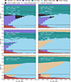 |
Fig. A.1. Outcomes of our detailed binary evolution models. The same as Fig.2 but for initial primary mass 5.0 M⊙, 6.3 M⊙, 7.9 M⊙, 10.0 M⊙, 12.6 M⊙, and 15.8 M⊙ |
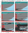 |
Fig. A.2. Outcomes of our detailed binary evolution models. The same as Fig. 2 but for initial primary mass 20.0 M⊙, 28.2 M⊙, 39.8 M⊙, 56.2 M⊙, 79.4 M⊙, and 100.0 M⊙. |
Appendix B: Supernova window
The SN windows, the initial parameter space allowing SNe to occur, play important roles by determining the magnitude of kick velocities. However, the resolution of our SMC model grid is not good enough to distinguish different types of SNe and we therefore adopted the SN windows computed by the ComBinE code (Kruckow et al. 2018, and Paper II) Taking ECSNe as an example, while ECSNe may happen in a very narrow mass range in single star case (Poelarends et al. 2008; Janka 2012), the ECSN window can be broadened by binary interaction (Podsiadlowski et al. 2004; Langer 2012; Shao & Li 2014; Poelarends et al. 2017; Siess & Lebreuilly 2018). However, detailed simulations show that even including mass transfer, it is still narrower than 1 M⊙ (Poelarends et al. 2017; Siess & Lebreuilly 2018). The ZAMS mass window computed by the ComBinE code is about [9.5, 10.2] M⊙. However, around this mass range, the SMC model grid only have three mass slices of 8.9 M⊙, 10 M⊙, and 11.22 M⊙. Instead of interpolating, we simply used our grid points to calculate the systems undergoing ECSNe with a factor accounting for the fraction of ECSNe in each pixel of our model grid. While this could cast uncertainties on our NS populations, it should be a minor effect comparing with merger criterion.
The fraction factor was calculated through the following approach. We used the ComBinE code simulates binaries with a flat distribution for the initial primary mass, M1, i, initial mass ratio, qi, and initial logarithmic orbital period, log Porb, i. Then we calculated the following statistical weight for all ComBinE models,
 (B.1)
(B.1)
where (α, β, γ) = (2.3, 0.1, 0.55) for our fiducial model (the Kroupa IMF and the Sana distribution), and (α, β, γ) = (2.3, 0, 0) for the logPq-flat model. With this statistical weight, we calculated the fraction of different types of SNe in each pixel of our SMC model grid. Taking ECSN as an example, the ECSN fraction, fECSN, was evaluated as
 (B.2)
(B.2)
where N is the total number of ComBinE models inside a given pixel from our MESA model grid, and
 (B.3)
(B.3)
The fractions of other types of SNe were calculated in the same way. In our population synthesis calculations, we used the Monte Carlo method to generate a sample of kick velocities with a size of n for each pre-SN systems, where n × fECSN of the sample were drawn from the kick distribution corresponding to ECSN.
Figure B.1 shows the ECSN fraction for each pixel in our model grid. We see that the ECSN window behaves differently in Case A/B systems. In Case B systems, mass transfer helps the donor star avoid the second dredge-up, which makes ECSNe become possible with relatively low stellar masses. In Case A systems, mass transfer happens when the primary stars are still on the main sequence, which limits the growth of the inner core in the post-MS evolution, and consequently the ZAMS mass window of ECSNe is shifted towards the high-mass end.
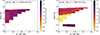 |
Fig. B.1. ECSN fraction on the qi − log Porb,i plane with initial primary mass 8.9 M⊙ and 10 M⊙. |
The ComBinE code like other rapid codes assumes that the envelope of donor star is completely stripped by mass transfer. With this assumption, Case BB or Case BC mass transfer only takes place in tight binaries. However, there could be a considerable fraction of envelope left after mass transfer at low metallicity (Laplace et al. 2020), which allows Case BB or Case BC mass transfer occur in wide binaries (Ercolino et al. 2024, 2025). We find a similar feature in our model grid. The remaining H-rich outer layer helps the core keep growing (Ercolino et al. 2024), which may shift the boundary between NS and WD. The H-rich outer layer can expand to very large radii and trigger the mass transfer from a partially stripped star. Usually, the partially stripped star is less massive than the accretor, making mass transfer widen the orbit. The parameter space of a helium-envelope-stripped SN could be narrowed by this process. In addition, due to the remaining material, stars could explode when they still fill their Roche lobe (Laplace et al. 2020; Ercolino et al. 2024, 2025). The asymmetric structure of pre-SN star may have effects on the kick velocities. We do not expect our predicted NS population to be largely affected by the difference in the physics in ComBinE and MESA.
Appendix C: Envelope inflation
Sanyal et al. (2015) have shown that in massive MS stars the maximum Eddington factor can exceed 1 inside the stars due to the Fe-bump of opacity. Radiation then pushes the envelope to a very large radius, leading to core-hydrogen burning supergiant models. Envelope inflation is sensitive to the treatment of convection and can cause convergence issues in calculation. The LMC binary models adopted in Langer et al. (2020b) cannot handle the effects of envelope inflation well and therefore do not have models with initial primary mass larger than about 40 M⊙. While envelope inflation can be avoided by assuming a more efficient energy transport inside the envelope (the MLT++ option in the MESA code Paxton et al. 2013), we do not see the reason to assume that the traditional mixing length theory becomes invalid (Böhm-Vitense 1958).
Since the inflated envelope is highly convective (Sanyal et al. 2015), Langer et al. (2020b) assume that the mass transfer from an inflated star is unstable. In our SMC models we do find the binaries undergoing envelope inflation reach the OB+BH phase. Above an initial primary mass of 50 M⊙, the effect of envelope inflation becomes more and more significant. As a consequence, the orbital period window of Case A systems significantly widens. With a more efficient convection, the inflated envelope will expend less and fill the Roche lobe at a later time, which could slightly increase the mass of the stripped star. Since there are only 11 OB+BH binaries having initial primary mass above 50 M⊙, we do not expect our result to be largely affected by this uncertainty.
Appendix D: Pair instability
We adopted the mass range and mass ejection of pulsational pair instability (PPI) computed by Marchant et al. (2019). None of our models are massive enough to produce pair-production SNe. Our 100 M⊙ single star model develops a helium core MHe, c of 58.6 M⊙ at the core helium depletion, which is still below the threshold for pair-production SNe (61.1 M⊙Marchant et al. 2019). Our fiducial model predicts 3.95 OB+BH binaries formed through PPI (hereafter PPI OB+BH), of which only 1 is significantly affected by the mass ejection during the PPI (MHe, c > 45 M⊙, Fig. 3). The recently updated 12C(α, γ)16O rate shifts the PPI mass range to a higher values (Farag et al. 2022), which would reduce our predicted number of PPI OB+BH binaries due to the effect of the IMF.
The PPI OB+BH binaries are also affected by the winds of WR stars, which are not well understood (Gräfener et al. 2017). In our binary model, primary stars with initial masses above ∼70 M⊙ can show a hydrogen-free WR star phase, during which the stellar winds reduce the masses of the WR stars. If our model had a weaker WR star wind, the predicted PPI OB+BH binaries would be slightly more eccentric due to a stronger mass ejection, while the total number of the PPI OB+BH binaries would not change. Given that the PPI OB+BH binaries only contribute a very small fraction to our synthetic population, we do not expect our result to be significantly affected by these uncertainties.
Appendix E: Calculations of statistical weights
We assumed the distribution of the initial mass of primary star is described by the initial mass function (IMF), which is fIMF ∝ M1,i−α, and the distributions of initial mass ratio and initial orbital period are fqi ∝ qi−β and flog Porb,i ∝ (log Porb,i)−γ. The predicted number contributed by a binary model Nb with initial parameter (M1,i, qi, log Porb,i) is
 (E.1)
(E.1)
In order to take into account star formation rate, we rewrote Eq. (E.1) into mass fraction form,
 (E.2)
(E.2)
Then from a constant star formation rate (SFR), the predicted number of a OB+cc binary was given by
 (E.3)
(E.3)
where V is the parameter space enclosed by [log Porb, i, log Porb, i + Δ log Porb, i], [qi, qi + Δqi], and [log M1, i, log M1, i + Δlog M1, i], (Δlog M1, i, Δqi, Δ log Porb, i) are the intervals of our model grid, lifetime is the lifetime of the OB+cc phase, and ⟨Mb⟩ is the averaged mass of the binary within the parameter space V weighted by the initial distributions, which is
 (E.4)
(E.4)
Defining statistical weight W as following,
 (E.5)
(E.5)
Eq. (E.3) has the following form
 (E.6)
(E.6)
In order to include non-constant star formation rate, we introduced the factor SFH,
 (E.7)
(E.7)
where the SFR is the function of lookback time, t, which means that t = 0 marks the observed status, ti/f, OB + cc are the binary age of entering/ending OB+cc phase. The observed OB+cc population at t = 0 comes from the star formation starting at t = tf, OB + cc and ending at t = ti, OB + cc. With this, the predicted number of a OB+cc binary with non-constant SFR is given by
 (E.8)
(E.8)
The number of O stars, He stars, and WR stars were computed with the same method except the lifetimes were determined by an effective temperature hotter than 31.6 kK, core helium burning, and core helium burning with a logarithmic luminosity higher than 5.6.
Appendix F: Tides during OB+cc phase
As is mentioned in Sect. 2.1, after the formation of BH or NS, we evolved the secondary as a single star. However, during the OB+cc phase, the OBe star can be spun down by tides. Here we toke into account tidal interaction by considering the synchronization timescale at the beginning of OB+cc phase. If the synchronization timescale is shorter than 10% of the lifetime of OB+cc phase8, we expect in the following OB+cc phase the OB star is rapidly spun down by tides and cannot form OBe stars.
In order to take into account the effect of eccentricity on tides, we introduced a different definition of synchronization timescale, τsync, basing on Hut (1981) and Hurley et al. (2002). The spin evolution of stars induced by tides was given by Hut (1981)
![Mathematical equation: $$ \begin{aligned} \frac{\mathrm{ d\, \Omega _\mathrm{ spin} }}{\mathrm{ d\, t}}=3\left(\frac{k}{T}\right)_\mathrm{rad} \left(\frac{q^2}{r_\mathrm{ g} ^2}\right)\left(\frac{R}{a}\right)^6 \frac{\Omega _\mathrm{ orb} }{(1-e^2)^6} \times \left[f_2(e^2) - (1-e^2)^{3/2}\,f_5(e^2)\frac{\Omega _\mathrm{ spin} }{\Omega _\mathrm{ orb} }\right], \end{aligned} $$](/articles/aa/full_html/2025/12/aa54786-25/aa54786-25-eq23.gif) (F.1)
(F.1)
where Ωorb and Ωspin are the orbital angular velocities and spin angular velocities of the OB star, mass ratio q is Mcc/ MOB, rg is the ratio of gyration radius to stellar radius R, e is eccentricity,
 (F.2)
(F.2)
the numerical factor E2 is
 (F.3)
(F.3)
f2(e2) and f5(e2) are defined by Hut (1981),
 (F.4)
(F.4)
and
 (F.5)
(F.5)
Basing on the above equations, we defined the synchronization timescale τsync as
![Mathematical equation: $$ \begin{aligned} \tau _\mathrm{sync} = \left|{\frac{\Omega _\mathrm{spin} - \Omega _\mathrm{ orb} }{\dot{\Omega }_\mathrm{ spin} } }\right| = \left[ 3 \left(\frac{k}{T}\right)_\mathrm{ rad} \left(\frac{q^2}{r_\mathrm{ g} ^2}\right)\left(\frac{R}{a}\right)^6\right]^{-1} \times \left|{\frac{(1-e^2)^6(\Omega _\mathrm{ spin} - \Omega _\mathrm{ orb} )}{f_2(e^2)\Omega _\mathrm{ orb} - (1-e^2)^{3/2}\,f_5(e^2)\Omega _\mathrm{ spin} }}\right|. \end{aligned} $$](/articles/aa/full_html/2025/12/aa54786-25/aa54786-25-eq28.gif) (F.6)
(F.6)
For circular orbit, e = 0, Eq. (F.6) becomes the widely used form
![Mathematical equation: $$ \begin{aligned} \tau _\mathrm{ sync} (e=0) = \left[ 3 \left(\frac{k}{T}\right)_\mathrm{ rad} \left(\frac{q^2}{r_\mathrm{ g} ^2}\right)\left(\frac{R}{a}\right)^6\right]^{-1}. \end{aligned} $$](/articles/aa/full_html/2025/12/aa54786-25/aa54786-25-eq29.gif) (F.7)
(F.7)
With the above assumption, we find that the tidal interaction during the OB+BH phase is too weak to spin down the OB stars. In our fiducial model, 170.401 OBe+BH binaries are predicted. Without tide, 170.403 OBe+BH binaries are predicted.
Appendix G: Further model details
G.1. Single star models
Figure G.1 presents the evolution of our non-rotating single star models. The evolution begins at the ZAMS point. After the MS phase, a hook appears due to the contraction before the ignition of hydrogen shell. About 50 M⊙, envelope inflation becomes more and more significant, which allows Case A mass transfer to occur in wide binaries. None of these single star models can produce WR stars through self-stripping.
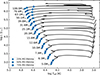 |
Fig. G.1. Evolutionary tracks of our non-interacting models in the Hertzsprung-Russell diagram, with the indicated initial masses. The tracks are terminated when the core helium abundance drops below 10−4. The circles, squares, and diamonds mark the ages of 25%, 50%, and 75% of the MS lifetime. |
G.2. An example of chemically homogeneous evolution model
All of our chemically homogeneous evolution models have a similar evolutionary history. Figure G.2 presents an example. The primary star is spun up by tide and evolves chemically homogeneously. As the primary star does not expand significantly, mass transfer is avoided. During the late hydrogen-burning phase, the primary star reaches the WR star regime, which is not considered in this work. When approaching the core helium ignition, the surface hydrogen rapidly drops to zero due to a enhanced stellar wind near the core hydrogen depletion.
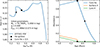 |
Fig. G.2. Example of our chemically homogeneous evolution model, with initial parameters indicated by text. The left panel presents the evolution of the chemically homogeneously evolving star on the Hertzsprung–Russell diagram, where the square and diamond mark helium ignition and the middle of helium burning. The right panel shows the chemical evolution of the chemically homogeneously evolving star as a function of its age. The blue, orange, and green correspond to the evolution of core helium, surface hydrogen, and core hydrogen. |
G.3. Properties of OB+WR binary systems
Figure G.3 presents the OB+WR binaries in the mass ratio MWR/MOB - logarithmic orbital period, log Porb, plane. Most of our OB+WR binaries have a MWR/MOB of 0.7. Below this value, binaries are formed with low initial orbital period and close-to-one initial mass ratio, where the mass gainer can accrete a large amount of mass. The number drop towards high log Porb is related to the initial distribution (cf. Sect. 3.4).
Figure G.4 presents the orbital velocities υorb, WR of the WR stars in the WR+O binaries. The observed SMC WR+O binaries have orbital periods Porb > 20 below 20 days and mass ratio MWR/MO below 0.6, and we accordingly divide our predicted population into three subpopulations, which are featured by Porb > 20 days, Porb < 20 days and MWR/MO > 0.6, and Porb < 20 days and MWR/MO < 0.6. The high-υorb, WR regime is dominated by the low-MWR/MO close WR+O binaries, which is the observed parameter space. Due to the change in mass ratios, the high-MWR/MO short WR+O binaries have lower υorb, WR, which is still above 100 km s−1. Most of our WR stars have an orbital velocity of about 50 km s−1, corresponding to wide systems (Porb > 20).
G.4. Properties of OB+cc binary systems
We further distinguish different modes of mass transfer (Case A or Case B). Case A systems produce the most massive O stars reaching 100 M⊙ and the slowest rotators, while Case B systems produce less massive OB stars and most of them are near-critically rotating (Fig. G.7). Case A systems usually have tight orbits, resulting in strong tidal interaction. As a result they have relative high accretion efficiency according to our rotation-dependent accretion efficiency. The opposite takes place in Case B systems, which results in near-zero accretion efficiency.
G.4.1. Masses and mass ratios
The top panel of Fig. G.5 shows the predicted distribution of MOB. The distribution peaks at ∼10 M⊙, below which stars have a lower chance of forming BHs or NSs. Above 10 M⊙ the number drop is due to the effects of the IMF and lifetime. Both BH systems and NS systems have a minimum companion mass about 6 M⊙ (cf. Sect. 3.3).
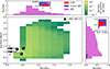 |
Fig. G.3. Predicted distribution of OB+WR binaries in the mass ratio, MWR/MOB, - logarithmic orbital period, log Porb, plane. The number in each pixel is coded in colour. The H-free and CHE WR stars are identified in 1D projection. The observed WR binaries (Foellmi et al. 2003; Foellmi 2004; Koenigsberger et al. 2014; Hainich et al. 2015; Shenar et al. 2016, 2018) are plotted with black. |
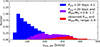 |
Fig. G.4. Predicted distribution of the orbital velocities υorb, WR of the WR stars in the WR+O binaries. Three subpopulations are identified, which are featured by Porb > 20 days (blue), Porb < 20 days and MWR/MO > 0.6 (purple), and Porb < 20 days and MWR/MO < 0.6 (observed region, red). The numbers of WR+O binaries correspond to each subpopulations are indicated by the text in the legend. |
The middle panel of Fig. G.5 shows the predicted distribution of MBH, which is mainly shaped by the IMF (cf. Sect. 3.6). In Case A systems, mass transfer begins when primary stars are still on the MS, which limits the growth of He core. Therefore, BH progenitors in Case A systems trend to have higher initial primary masses than that in Case B systems. Towards the high-mass end, the orbital period window of Case A binaries becomes wider and wider due to the increasing importance of envelope inflation. These wide-orbit Case A systems produce the most massive BHs, which can have fast-rotating companions because of weak tide.
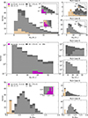 |
Fig. G.5. Top panel: Distributions of OB star masses, MOB, in OB+cc binaries. The types of compact objects are colour-coded (BH: black, NS: brown), and the shaded area is related to the OBe feature. The OB+BH binaries formed from CHE are plotted with purple. The number in the legends is the predicted number of OBe stars and normal OB stars, e.g. ‘Black hole: 170+41’ means 170 BH+OBe binaries and 41 BH+OB binaries. The in-layer plot in the top panel shows the distribution in the range 30 - 100 M⊙ with bin width of 10 M⊙, while the main plot is produced in 6 - 30 M⊙ with bin width of 2 M⊙. The left panel is the distribution of the total population, which is disentangled into Case A systems and Case B systems in the right upper and lower panel, respectively. Middle panel: Distributions of BH masses. Bottom panel: Distributions of mass ratios of OB+cc binaries. |
The bottom panel of Fig. G.5 presents the distribution of mass ratio of OB+cc binaries (q = Mcc/MOB). In our calculations, the mass of NS was fixed to be 1.4 M⊙, while most of their companions have mass around 10 M⊙, leading to a peak in mass ratio at ≃0.1. Since our model predicts all OB stars in OB(e)+NS binaries to be more massive than 6 M⊙, the highest mass ratio of NS systems is about 0.2-0.3.
The mass ratio of OB+BH binaries peaks at ≃0.6-0.7, clearly separated from the NS systems. The drop in numbers towards high mass ratio is due to the increasing fraction of the binaries undergoing unstable mass transfer. The effects of decreasing lifetime cause the number drop towards a low mass ratio. Case A systems contribute the lowest mass ratio ∼0.2 and highest mass ratio ∼1.8, corresponding to close binaries with high accretion efficiency and wide binaries with inflated primary stars, respectively.
G.4.2. Orbital properties
The top panel of Fig. G.6 shows the distribution of orbital periods of OB+cc binaries Porb. Our merger criterion leads to a peak near Porb = 100 days (cf. Sect. 3.6), which is dominated by Case B systems. Case A systems require close orbits, leading to a peak near 7 days. A small fraction of Case A systems have orbital periods above 100 days due to envelope inflation (BH binaries) or SN kick (NS binaries).
The bottom panel of Fig. G.6 shows the distribution of the semi-amplitude of orbital velocities of OB stars, KOB. For BH systems, the KOB distribution peaks at 30–40 km s−1, corresponding to Case B systems. Case A systems peaks at 80–90 km s−1 since them have closer orbits. For NS systems, the OB stars are much more massive than the NSs, making KOB less than 30 km s−1. A few NS binaries have KOB > 200 km s−1 due to their high eccentricity.
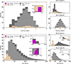 |
Fig. G.6. Top panel: Distribution of logarithmic orbital periods, log Porb, of OB+cc binaries. The colours and legends have the same meaning as in Fig. G.5. Lower panel: Semi-amplitude of orbital velocity of OB stars, KOB. |
G.4.3. Rotation of OB stars
Figure G.7 presents the distribution of rotational velocity υrot of OB stars (top panel), which shows a fast-rotating peak around 600 km s−1 with a slow-rotating tail extended to 100 km s−1. The fast-rotating peak reflect the critical rotation velocities of stars with mass around 10 M⊙. In Case A systems, tidal interaction plays an important role, which makes υrot distributed in 100 − 600 km s−1. We notice that some Case A BH and NS binaries can rotate critically. For BH binaries, these critically rotating systems have inflated primary stars and wide orbit. For NS binaries, the stripped star could not be massive enough to spin down the mass gainer.
We further present the distribution of the ratio of rotational velocity to critical velocity, υrot/υcrit, in the bottom panel of Fig. G.7. Similar with the top panel, the υrot/υcrit ratio shows a fast-rotating peak at 1 with a slow-rotating tail extended to 0.2, corresponding to Case B and Case A systems. In Case B systems, most of binaries have υrot/υcrit > 0.95 as expected, while 18 of them with υrot/υcrit < 0.95 are braked by stellar wind.
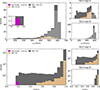 |
Fig. G.7. Distribution of rotation velocities of OB stars, υrot (top), and ratios of rotation velocity to critical velocity, υrot/υcrit, of OB stars (bottom). The colours and legends have the same meaning as in Fig. G.5 |
G.4.4. Surface abundance of OB stars
We present the predicted distribution of surface abundance of OB stars in Fig. G.8. Surface abundance can be enriched through two ways, internal mixing and mass transfer. For He, it is mainly enriched by mass transfer because the strong gradient in mean molecular weight between the core and the envelope prevents the transfer of He. Due to the near-zero accretion efficiency of wide binaries, most of OB stars have He unenriched. When the second mass transfer episode takes place, some accretors rotate sub-critically due to wind braking, allowing their surface He to be slightly enriched. In Case A systems, due to the effect of tidal braking, accretion efficiency can be up to 60%. Consequently, the most enriched star has surface helium mass fraction about 0.5. The unenriched Case A binaries have inflated primary stars.
The distribution of surface nitrogen enhancement factor (surface nitrogen mass fraction divided by initial surface nitrogen mass fraction) is presented in the lower panel of Fig. G.8. Different from helium, surface nitrogen can be enriched by both mixing and mass transfer because CN-equilibrium is reached before the establishment of the strong gradient in mean molecular weight so that nitrogen in core can be transferred throughout envelope. In Case B systems, surface nitrogen is mainly enriched by internal mixing, resulting in an enrichment factor of about 2-3. In Case A systems, the unenriched peak is related to the effect of envelope inflation and mass transfer leads to an enrichment factor of 10 to 15. Hastings et al. (2020) show that the surface abundance of nitrogen is sensitive with initial rotation velocity. An initially fast-rotating star can have its surface nitrogen enriched by a factor of 30. In our models, all secondary stars are initially slow rotators. Hence our results give an lower limit on the nitrogen enhancement.
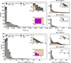 |
Fig. G.8. Distributions of surface mass fraction of 4He X4He, surf (top panel) and the enhancement factor of 14N X14N, surf/ initial X14N, surf (bottom panel) of OB stars. The colours and legends have the same meaning as in Fig. G.5. |
All Tables
Predicted numbers of the pre- and post-interaction MS OB stars in our fiducial synthetic SMC population.
Number of post-MS companions of OB stars in our fiducial synthetic SMC population.
All Figures
|
Fig. 1. Schematic evolution of a massive binary system through the six evolutionary phases considered in this paper: pre-interaction, RLO, stripped envelope star (subdwarf, helium star, or Wolf-Rayet star), compact object, referred to as the compact companion (cc) in a binary system, formation possibly connected with a SN explosion, X-ray silent compact object binary, and HMXB. After the second stage, a fraction of the mass gainers may be fast-rotating and appear as Oe or Be stars, and after NS formation as a OBe X-ray binary. Notably, many systems do not survive the second, fourth, and sixth stage as a binary, i.e. the number of systems evolving from top to bottom is being reduced at these stages. The figure is adapted from Kruckow et al. (2018). |
| In the text | |
|
Fig. 2. Outcome of the first mass transfer phase in our detailed binary evolution models with an initial primary mass of 17.8 M⊙. In this figure, each pixel represents one detailed MESA binary evolution model, and the corresponding evolutionary outcome is colour-coded (see top legend). Here, ‘OB+cc’ (cc= BH, NS, WD) implies that the corresponding model produced an OB+cc phase, with the cc type indicated by the corresponding colour. However, depending on the adopted compact object birth kicks, these systems may also break up. Systems indicated as ‘Upper_mdot_limit’ or ‘MT_max’ are terminated during their first mass transfer phase as the mass transfer rate exceeds limiting values (see text) and a merger is expected, and those indicated as ‘other merger’ undergo L2-overflow in a contact situation. Corresponding plots for different initial donor star masses can be found in Appendix A. |
| In the text | |
|
Fig. 3. Remaining mass, Mrem, after the pulsations triggered by pair instability, as a function of the helium core mass, MHe, c, at core helium depletion. The grey and blue lines correspond to the model data in Marchant et al. (2019) and Eq. (3), respectively. The red line shows the relation Mrem = MHe, c. |
| In the text | |
|
Fig. 4. Predicted distribution of OB stars with a NS (left panel) and BH (right panel) companion in the Hertzsprung–Russell diagram. The green line is the ZAMS, and the black line is the terminal-age main sequence (TAMS). The blue lines represent evolutionary tracks of non-rotating core hydrogen burning single stars, with the indicated initial masses. The dashed red lines show the boundaries of the three groups of stars defined in the main text, i.e. Teff = 31.6 kK, log L/L⊙ = 5, and the MS evolutionary track of a 8.9 M⊙ single star. On top, we label several spectral types at their approximate effective temperature. |
| In the text | |
|
Fig. 5. Pie charts for the predicted numbers of pre-interaction MS OB stars primaries, and of OB stars in different types of post-interaction binaries, divided into three groups, Group 1 (top left; top right provides a zoom-in), Group 2 (lower left), and Group 3 (lower right), based on luminosities and effective temperatures. The considered types of binary stars and the corresponding fractions with respect to the total number within the considered group are indicated by text. The corresponding absolute numbers in each wedges are listed in Table 2. |
| In the text | |
|
Fig. 6. Fractions of different types of post-MS companions of OB stars in our fiducial synthetic binary population relative to all post-MS companions, as a function of the mass of the OB star. For the companions, we distinguish core-helium burning stars (magenta), white dwarfs (blue), NSs (yellow), and BHs (grey). Shading identifies those companions that are paired with an OB star that rotates with more than 95% of its critical rotational velocities. The absolute number of binaries with post-MS companions expected in the SMC for each mass bin is given on top of the bin. The high-mass end (30–100 M⊙) is presented with a wider bin width. |
| In the text | |
|
Fig. 7. Distributions of properties of the predicted SMC OB+WR binary population. The top panel shows the distribution of the predicted position of the WR components in the Hertzsprung Russell diagram (background colours), where the colour indicates the expected number per pixel (see colour bar on the top right). The total number of observed WR star components, or WR binaries, is four. The plots to the right and on top give the 1D-projections of the distribution, with the inset magnifying the WR binaries produced via chemical homogeneous evolution (CHE). The black circles and diamonds represent the WR components of the observed WR binaries, and single WR stars, in the SMC (Foellmi et al. 2003; Foellmi 2004; Koenigsberger et al. 2014; Hainich et al. 2015; Shenar et al. 2016, 2018), where the numbers are related to the identifier, e.g. ‘1’ for ‘SMC AB1’. The dashed blue line is the zero-age main sequence of helium star models (He-ZAMS) with SMC metallicity (Köhler et al. 2015), with the indicated helium star masses. The bottom panel shows the distribution of the predicted WR binaries in the plane of orbital period versus the orbital velocity of the WR component. Here, the black symbols represent the projected orbital velocity semi-amplitudes of the observed WR+O star binaries (circles) and of the WR+WR binary SMC AB5 (diamond). |
| In the text | |
|
Fig. 8. Distributions of the orbital periods of the ∼25 OB+NS binaries in our fiducial synthetic SMC population. Upper left: Predicted period distribution (yellow histogram), where the ∼21 OB+NS binaries in which the OB stars rotates faster than 95% of their critical rotational velocity are indicated by shading (labelled ‘OBe’). The period distribution of observed BeXBs in the SMC (Haberl & Sturm 2016) is plotted as purple line. Upper right: A zoom-in of the upper left panel. The B star + radio pulsar binary J0045-7319 (Bell et al. 1995) and the supergiant X-ray binary SMC X-1 (Rawls et al. 2011; Falanga et al. 2015) are indicated by arrows. Lower left: The same predicted distribution as in the top panels, with the colours indicating which of the systems formed through Case A and Case B mass transfer (blue and orange, respectively), with the corresponding total numbers given in the legend. Lower right: The same predicted distribution as in the top panels, with the colours indicating which type of SN, and therefore which NS kick distribution, was assumed for the different systems [green for electron-capture SN; red for helium-envelope-stripped SN (CCSN-C); purple for hydrogen-envelope-stripped SN (CCSN-He); cf. Sect. 2.6]. The predicted total numbers related to different SN types are given in the legend. |
| In the text | |
|
Fig. 9. Distribution of the eccentricities of our OB+NS model binaries, with the colours indicating which type of SN was assumed for the different systems, as in the bottom right panel of Fig. 8. |
| In the text | |
|
Fig. 10. 2D distribution of the ∼24 OB+NS binaries of our fiducial synthetic SMC population in the orbital period – eccentricity plane. The number in each pixel is colour-coded. The 7 SMC BeXBs with eccentricity measurements (Townsend et al. 2011; Coe & Kirk 2015) are indicated by black diamonds. The B star + radio pulsar binary (Kaspi et al. 1994; Bell et al. 1995) is marked by a black star, the supergiant X-ray binary SMC X-1 by a black triangle (Falanga et al. 2015). |
| In the text | |
|
Fig. 11. Properties of the ∼211 OB+BH binaries in our fiducial synthetic SMC population (cf. Table 3), as function of the mass of the OB star. The three main plots show the 2D number density distributions of the systems, with the OB star mass on the X axis, and BH mass, orbital period, and OB star orbital velocity semi-amplitude on the Y axis, respectively. The number density is colour coded (see colour bar on the top right). The known OB+BH binaries, irrespective of their host galaxy metallicity, are marked by blue symbols, and correspond to MWC 656 (Casares et al. 2014), Cyg X-1 (Miller-Jones et al. 2021), LMC X-1 (Orosz et al. 2009), M33 X-7 (Ramachandran et al. 2022), VFTS 243 (Shenar et al. 2022a), and HD 130298 (Mahy et al. 2022). The BH nature of the secondary star in MWC 656 debated in the literature. The solution by Janssens et al. (2023) is labelled by ‘MWC 656 (new)’ and connected to the solution by Casares et al. (2014) through a red line. The four histograms give the corresponding 1D projections, with shading identifying rapidly rotating OB stars (labelled ‘OBe’), and insets magnifying the small contributions from chemically homogeneous evolution (CHE). The orbital velocity semi-amplitudes for observed systems are calculated using Eq. (11) with the observed masses and orbital periods. The errors are calculated by error propagation. |
| In the text | |
|
Fig. 12. Orbital period (left plots) and V band magnitude or mass (right) distributions of the OB+NS (top) and OB+BH (bottom) binaries resulting from our parameter variations. The predictions from the different population models are shown with differently coloured lines (see legend), where the predictions from the fiducial model are indicated by the hatched histograms with blue thick lines. The population models that produce the same distributions as the fiducial model are not shown in the corresponding plots. In the bottom plots, the SFH-R distributions are very close to the fiducial ones. We show the distributions of the observed SMC BeXBs in the upper panels with grey histograms. The observed orbital periods and V-band magnitudes of the SMC BeXBs are from Haberl & Sturm (2016). |
| In the text | |
|
Fig. 13. Star formation history adopted to compute the population models SFH-S (upper panel, Schootemeijer et al. 2021) and SFH-R (lower panel, Rubele et al. 2015), where the dashed line indicates the constant star formation rate of 0.05 M⊙ yr−1 used in the fiducial model. |
| In the text | |
|
Fig. 14. Predicted fraction of OBe stars in our fiducial synthetic SMC population as a function of apparent Gbp magnitude (blue). The OB stars in pre-interaction binaries are included. The observed OBe star fraction is plotted with red (Schootemeijer et al. 2022). On the top we show the averaged evolutionary mass in each bin (Schootemeijer et al. 2022). |
| In the text | |
|
Fig. A.1. Outcomes of our detailed binary evolution models. The same as Fig.2 but for initial primary mass 5.0 M⊙, 6.3 M⊙, 7.9 M⊙, 10.0 M⊙, 12.6 M⊙, and 15.8 M⊙ |
| In the text | |
|
Fig. A.2. Outcomes of our detailed binary evolution models. The same as Fig. 2 but for initial primary mass 20.0 M⊙, 28.2 M⊙, 39.8 M⊙, 56.2 M⊙, 79.4 M⊙, and 100.0 M⊙. |
| In the text | |
|
Fig. B.1. ECSN fraction on the qi − log Porb,i plane with initial primary mass 8.9 M⊙ and 10 M⊙. |
| In the text | |
|
Fig. G.1. Evolutionary tracks of our non-interacting models in the Hertzsprung-Russell diagram, with the indicated initial masses. The tracks are terminated when the core helium abundance drops below 10−4. The circles, squares, and diamonds mark the ages of 25%, 50%, and 75% of the MS lifetime. |
| In the text | |
|
Fig. G.2. Example of our chemically homogeneous evolution model, with initial parameters indicated by text. The left panel presents the evolution of the chemically homogeneously evolving star on the Hertzsprung–Russell diagram, where the square and diamond mark helium ignition and the middle of helium burning. The right panel shows the chemical evolution of the chemically homogeneously evolving star as a function of its age. The blue, orange, and green correspond to the evolution of core helium, surface hydrogen, and core hydrogen. |
| In the text | |
|
Fig. G.3. Predicted distribution of OB+WR binaries in the mass ratio, MWR/MOB, - logarithmic orbital period, log Porb, plane. The number in each pixel is coded in colour. The H-free and CHE WR stars are identified in 1D projection. The observed WR binaries (Foellmi et al. 2003; Foellmi 2004; Koenigsberger et al. 2014; Hainich et al. 2015; Shenar et al. 2016, 2018) are plotted with black. |
| In the text | |
|
Fig. G.4. Predicted distribution of the orbital velocities υorb, WR of the WR stars in the WR+O binaries. Three subpopulations are identified, which are featured by Porb > 20 days (blue), Porb < 20 days and MWR/MO > 0.6 (purple), and Porb < 20 days and MWR/MO < 0.6 (observed region, red). The numbers of WR+O binaries correspond to each subpopulations are indicated by the text in the legend. |
| In the text | |
|
Fig. G.5. Top panel: Distributions of OB star masses, MOB, in OB+cc binaries. The types of compact objects are colour-coded (BH: black, NS: brown), and the shaded area is related to the OBe feature. The OB+BH binaries formed from CHE are plotted with purple. The number in the legends is the predicted number of OBe stars and normal OB stars, e.g. ‘Black hole: 170+41’ means 170 BH+OBe binaries and 41 BH+OB binaries. The in-layer plot in the top panel shows the distribution in the range 30 - 100 M⊙ with bin width of 10 M⊙, while the main plot is produced in 6 - 30 M⊙ with bin width of 2 M⊙. The left panel is the distribution of the total population, which is disentangled into Case A systems and Case B systems in the right upper and lower panel, respectively. Middle panel: Distributions of BH masses. Bottom panel: Distributions of mass ratios of OB+cc binaries. |
| In the text | |
|
Fig. G.6. Top panel: Distribution of logarithmic orbital periods, log Porb, of OB+cc binaries. The colours and legends have the same meaning as in Fig. G.5. Lower panel: Semi-amplitude of orbital velocity of OB stars, KOB. |
| In the text | |
|
Fig. G.7. Distribution of rotation velocities of OB stars, υrot (top), and ratios of rotation velocity to critical velocity, υrot/υcrit, of OB stars (bottom). The colours and legends have the same meaning as in Fig. G.5 |
| In the text | |
|
Fig. G.8. Distributions of surface mass fraction of 4He X4He, surf (top panel) and the enhancement factor of 14N X14N, surf/ initial X14N, surf (bottom panel) of OB stars. The colours and legends have the same meaning as in Fig. G.5. |
| In the text | |
Current usage metrics show cumulative count of Article Views (full-text article views including HTML views, PDF and ePub downloads, according to the available data) and Abstracts Views on Vision4Press platform.
Data correspond to usage on the plateform after 2015. The current usage metrics is available 48-96 hours after online publication and is updated daily on week days.
Initial download of the metrics may take a while.