| Issue |
A&A
Volume 704, December 2025
|
|
|---|---|---|
| Article Number | A125 | |
| Number of page(s) | 20 | |
| Section | Extragalactic astronomy | |
| DOI | https://doi.org/10.1051/0004-6361/202555556 | |
| Published online | 05 December 2025 | |
Torus feeding and outflow launching in the active nucleus of the Circinus galaxy
1
Leiden Observatory, University of Leiden, PO Box 9513, 2300 RA Leiden, The Netherlands
2
European Southern Observatory, Alonso de Córdova 3107, Vitacura, Santiago, Chile
3
Institute ASTRON, Netherlands Institute for Radio Astronomy, NL-7991 PD Dwingeloo, The Netherlands
4
Instituto de Estudios Astrofísicos, Universidad Diego Portales, Av. Ejírcito Libertador 441, Santiago, Chile
5
School of Astronomy and Space Science, Nanjing University, 163 Xianlin Avenue, Nanjing 210023, People’s Republic of China
6
School of Astronomy and Space Science, Nanjing University, Nanjing 210093, China
7
Key Laboratory of Modern Astronomy and Astrophysics (Nanjing University), Ministry of Education, Nanjing 210093, China
⋆ Corresponding author: This email address is being protected from spambots. You need JavaScript enabled to view it.
Received:
16
May
2025
Accepted:
23
September
2025
Abstract
Context. Most active galactic nuclei (AGNs) are believed to be surrounded by a dusty molecular torus on the parsec scale, which is often embedded within a larger circumnuclear disc (CND). Active galactic nuclei are fuelled by the inward transport of material through these structures and can launch multi-phase outflows that influence the host galaxy through AGN feedback.
Aims. We use the Circinus galaxy as a nearby laboratory to investigate the physical mechanisms responsible for feeding the torus and launching a multi-phase outflow in this Seyfert-type AGN, as these mechanisms remain poorly understood.
Methods. We analysed observations from the Atacama Large Millimeter/submillimeter Array of the Circinus nucleus at angular resolutions down to 13 mas (0.25 pc). We traced dust and the ionised outflow using 86 − 665 GHz continuum emission and studied the morphology and kinematics of the molecular gas using the HCO+(3-2), HCO+(4-3), HCN(3-2), HCN(4-3), and CO(3-2) transitions.
Results. We find that the Circinus CND hosts molecular and dusty spiral arms, two of which connect directly to the torus. We detect inward mass transport along these structures and argue that the non-axisymmetric potential generated by these arms is the mechanism responsible for fuelling the torus. We estimate a feeding rate of 0.3 − 7.5 M⊙ yr−1, implying that over 88% of the inflowing material is expelled in a multi-phase outflow before reaching the accretion disc. The inferred feeding timescale (tfeed, torus = 120 kyr − 2.7 Myr) suggests that variability in AGN activity may be driven by changes in torus feeding. On parsec scales, the ionised outflow is traced by optically thin free-free emission. The outflow is stratified, with a slightly wider opening angle in the molecular phase than in the dusty and ionised components. The ionised outflow is launched or collimated by a warped accretion disc at a radius of r ∼ 0.16 pc, and its geometry requires an anisotropic launching mechanism.
Key words: galaxies: active / galaxies: ISM / galaxies: individual: Circinus / galaxies: kinematics and dynamics / galaxies: nuclei / galaxies: Seyfert
© The Authors 2025
 Open Access article, published by EDP Sciences, under the terms of the Creative Commons Attribution License (https://creativecommons.org/licenses/by/4.0), which permits unrestricted use, distribution, and reproduction in any medium, provided the original work is properly cited.
This article is published in open access under the Subscribe to Open model. This email address is being protected from spambots. You need JavaScript enabled to view it. to support open access publication.
1. Introduction
The Circinus galaxy hosts the nearest Seyfert 2 active galactic nucleus (AGN), located at a distance of ∼4 Mpc (1″ ∼ 20 pc). Active galactic nuclei are powered by the release of gravitational energy from material accreting onto a supermassive black hole (SMBH). This energy is released in the form of X-rays, UV radiation, and multi-phase outflows, including relativistic jets and molecular, dusty, and ionised winds. Through interactions with the surrounding medium, this energy output can profoundly influence the evolution of the host galaxy in a process known as AGN feedback (see e.g. Harrison & Ramos Almeida 2024 and references therein). Understanding the physical mechanisms that fuel and regulate AGN activity is therefore critical for constraining models of coevolution between SMBHs and their host galaxies. Nearby AGNs, such as in the Circinus galaxy, offer a unique laboratory for investigating these mechanisms in detail.
In the inner regions of Circinus, an accretion disc surrounding the SMBH can be traced accurately by H2O megamasers (Greenhill et al. 2003), revealing a significant warp at sub-parsec scales and a SMBH mass of M• = 1.7 × 10⁶ M⊙. Combined with a bolometric luminosity of Lbol = 4 × 1043 erg s−1 (Moorwood et al. 1996), this implies an Eddington ratio of ∼20%. Outside of this accretion disc, AGNs are believed to contain a cold molecular dusty torus that surrounds it and can hide the high-energy radiation that is emitted by the accretion disc (Krolik & Begelman 1986; Antonucci 1993; Urry & Padovani 1995). Due to their small sizes, AGN tori can only be resolved at the highest angular resolutions, such as with the Atacama Large Millimeter/submillimeter Array (ALMA). Such observations yield information about their geometry, chemistry, and dynamics (García-Burillo et al. 2016; Izumi et al. 2018; Combes et al. 2019; Impellizzeri et al. 2019).
Because Circinus is a type 2 Seyfert (Oliva et al. 1994), we observe this torus edge-on (Izumi et al. 2023, hereafter I23; Baba et al. 2024), which means that the broad-line region is obscured from our view. As a result, we observe radiation that has been reprocessed by the structures surrounding the hot inner region of the AGN in the infrared (IR) and sub-millimetre regime (Storchi-Bergmann et al. 1992). In the nucleus, the dominant mid-IR emitting structure is the dusty biconical outflow, which is perpendicular to the maser disc and has a size of ∼2 pc (Tristram et al. 2007; Isbell et al. 2022). The ionised outflow, which is launched from the inner parsec region, is observed as a one-sided outflow cone in [O III] out to ∼400 pc and as a two-sided plume in the radio out to ∼1 kpc (Marconi et al. 1994; Elmouttie et al. 1998). Surrounding these AGN tori, we often find a circumnuclear disc (CND) that consists of cold molecular gas and dust. In the Circinus galaxy, the CND directly surrounds the torus. The torus and CND act as mass reservoirs from which AGNs are fuelled (Combes 2021b).
High-resolution ALMA observations pave the way towards resolving some long-standing questions. From statistical studies of the obscuration fractions in AGNs, we know, for example, that tori must have scale heights of h/r ∼ 1. However, the mechanism that keeps these tori geometrically thick remains unknown. The proposed mechanisms include supernova explosions within the torus (Wada & Norman 2002), radiation pressure from the thin disc (Pier & Krolik 1992), magnetically driven outflows that sweep up obscuring material (Emmering et al. 1992), and the radiation-driven fountain model in which turbulence is injected into the torus by the backflow of the molecular outflow (Wada 2012). Other important open questions include the feeding mechanism that transports material from the CND down to the torus (Combes 2021a) and the launching mechanism of the ionised, dusty, and molecular outflows, which could, for example, be driven by radiation pressure (Dorodnitsyn et al. 2011; Chan & Krolik 2016; Hönig & Kishimoto 2017) or by magnetocentrifugal forces (Vollmer et al. 2018). The aim of this work is to use the Circinus AGN as a laboratory to study torus feeding and outflow launching in a prototypical Seyfert 2 type AGN.
2. Observations and data reduction
2.1. Observations
We obtained data from ALMA band 6 (259 GHz, 1.16 mm) and band 7 (350 GHz, 0.86 mm) of the Circinus nuclear region (project code 2018.1.00581.S, PI: K. Tristram). In band 6, short baseline (beam ∼2 pc) observations – referred to as ‘B6SB’ – were obtained in addition to long baseline data (B6LB, beam ∼0.4 pc). In band 6, we targeted the HCO+(3-2) and HCN(3-2) transitions, while in band 7, we targeted HCO+(4-3), HCN(4-3) and CO(3-2). In addition, we used auxiliary datasets in bands 3 (86 GHz & 99 GHz), band 4 (135 GHz & 147 GHz), band 5 (178 GHz) and band 9 (665 GHz) (project codes 2017.1.00575.S, PI: J. Wang and 2019.1.00013.S, PI: V. Impellizzeri) to investigate the spectral energy distribution (SED). We list observational details in Tables 1 and A.1 for the primary and auxiliary datasets.
Observation and data reduction details of the primary datasets..
2.2. Data reduction
We performed the data reduction using the Common Astronomy Software Applications (CASA, The CASA Team 2022) to produce continuum and molecular emission maps. For band 6 and 7, we applied standard pipeline calibration (version listed in Table 1) using J1424-6807 as the bandpass calibrator and J1427-4206 as the phase and amplitude calibrator. We then applied several rounds of phase self-calibration on the continuum followed by one amplitude calibration – except for the band 7 data due to an insufficient signal-to-noise ratio (S/N). We found that self-calibration increases the S/N by a factor of 9.9, 1.35, and 1.17 in the B6SB, B6LB, and B7 datasets, respectively. After self-calibration, we subtracted the continuum emission using ‘fitorder = 0’ in the ‘imcontsub’ casa task. Since the B6LB and B7 datasets were split into two separate observing epochs, we combined these epochs into a single measurement set using the ‘concat’ task in CASA. We also explored the possibility of combining B6SB with B6LB, but decided not to do this due to an offset of ∼30 mas between the peak of the continuum of B6SB and those of B6LB and B7 (see Sect. 3.4).
We then imaged the datasets using the ‘tclean’ casatask with auto-masking1, velocity bins of 10.2 km s−1 for B6SB and 7.6 km s−1 for B6LB and a cell size of 3 mas. We used Briggs weighting with robust parameters of 0.5 and 2.0 for the continuum and molecular emission maps, respectively, to optimise the S/N and resolution. In addition, we cleaned the B6LB continuum using a robust parameter of -1.0 to image the continuum morphology at a beam size of only 14.3 × 12.2 mas2. After imaging, we applied primary beam correction to all maps, which boosted the flux density by less than one percent at the edge of the image. Lastly, we created moment-zero maps from the molecular line data cubes using the software CARTA (Comrie et al. 2018).
3. Results
3.1. Continuum emission
We present the continuum maps of B6LB and B6SB at 259 GHz in Fig. 1. We do not show the B7 continuum here, since its morphology is very similar to that of B6. An overview of all continuum maps between 86 GHz and 665 GHz is presented in Fig. A.1. The short baseline data of B6 show an unresolved core that is immediately surrounded by a ∼10 pc long elongated component with a position angle (PA) of ∼130°. This direction matches the PA of the dusty outflow on the parsec scale (Stalevski et al. 2019) and the one-sided ionised outflow cone that extends to ∼1 kpc (Marconi et al. 1994; Kakkad et al. 2023). We refer to this as the polar direction, as indicated in Fig. 1. Toward the south-east, we observe an elongated component along this polar axis that extends to a projected distance of ∼8 pc from the AGN. We refer to this structure as the ‘Phoenix’2 (white arrow in Fig. 1). The nuclear core is unresolved with short baselines and shows a flux density of 23.3 mJy but is resolved by the long baseline data in band 6 into a central peak of 14.6 mJy with extended polar structure. Following the levels of the continuum contours inward from ∼10 pc to the unresolved 0.4 pc core, we observe a clockwise rotation. The contours rotate from the polar direction (PA ∼ 130°) in B6SB to a ∼3 pc long horizontal bar (PA ∼ 92°) in B6LB and eventually to the equatorial direction (PA ∼ 45°, as indicated in Fig. 1) at the parsec scale.
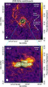 |
Fig. 1. Band 6 short (top) and long (bottom) baseline continuum maps at 259 GHz. Contour levels are drawn at [2, 4, 8, 16, 32, 64, 128, 256, 512, 1024] × rms, where the background rms equals 0.022 mJy/beam in the B6SB map and 0.013 mJy/beam in the B6LB map. The synthesised beam sizes are drawn in the bottom left as filled ellipses, and the cyan cross indicates the AGN position (as defined in Sect. 3.4). The phoenix feature is indicated with a white arrow. The polar and equatorial directions mentioned throughout the text are shown in the upper panel. |
On an arc second scale, we observe the CND which traces an S shape and closely matches the morphology of the molecular CND. To the north-east, we detect a spiral arm that extends out to ∼30 pc and connects to the CND. These extended structures are visible in bands 6, 7, and 9, but are not detected at lower frequencies despite similar sensitivities (see Fig. A.1).
3.2. Molecular line emission
We present the CO(3-2) molecular map zoomed in on the CND in Fig. 2 and show the HCO+(3-2) and HCN(3-2) maps in Fig. 3. In addition, we present the HCO+(4-3), HCN(4-3) and CO(3-2) maps in Fig. A.2. The HCO+(3-2) and HCN(3-2) transitions trace dense molecular gas (ncrit, HCO+(3 − 2) = 1.0 × 106 cm−3 and ncrit, HCN(3 − 2) = 5.7 × 106 cm−3 at Tkin = 50 K, Shirley 2015), while CO(3-2) traces slightly lower-density molecular gas (ncrit, CO(3 − 2) ≈ 1.7 × 104 cm−3 at Tkin = 50 K)3.
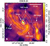 |
Fig. 2. Spiral structures in the CND (as informed by the morphology in Figs. 3 and A.2) overlaid on the band 7 CO(3-2) (νrest = 345.8 GHz) map. The dashed cyan arrow represents the proposed inflow through the NW hook that feeds the torus as discussed in Sect. 4.5. The synthesised beam size is drawn in the bottom left as a filled ellipse, and the cyan cross indicates the AGN position. |
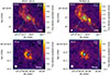 |
Fig. 3. Band 6 HCO+(3-2) (νrest = 267.6 GHz) and HCN(3-2) (νrest = 265.9 GHz) short (top, covering the CND) and long (bottom, showing the resolved torus) baseline moment zero maps. Contour levels are drawn at [ − 16, −8, −4, 2, 4, 8, 16] × rms, where the background rms equals 36, 23, 57 and 28 mJy/beam km/s in the HCO+(3-2) B6SB and B6LB and HCN(3-2) B6SB and B6LB maps, respectively. White contours represent negative flux density values and indicate the position of an absorption hole that coincides with the continuum peak. The L-shape that contains the NW and SW hooks as discussed in the text is drawn as dashed black lines in the top panels. Cyan contours in the top panels indicate the position of the blueshifted emission feature discussed in Sect. 4.5 and represent the −30 km s−1 level in the right panels of Fig. 8. The synthesised beam sizes are drawn in the bottom left as filled ellipses, and the cyan cross indicates the AGN position. |
On a scale of ≳10 pc, the dense molecular gas traces a morphology that is very similar to that of the B6SB continuum, except for the Phoenix, which is absent from the molecular maps. At the centre of the CND, we find the molecular torus, which is viewed almost edge-on (inclination of i ∼ 85° as determined by Baba et al. 2024 and I23). We measure the projected size of the torus to be approximately 120 × 90 mas2 or 2.4 × 1.8 pc2 from the HCO+ disc, which appears slightly more extended than the HCN disc. The emission from this edge-on torus resembles that of an oblate disc with an ‘absorption hole’ at the centre that coincides with the continuum peak, as also described by (I23). In the lower-resolution HCO+(4-3), HCN(4-3) and CO(3-2) maps, we detect a local reduction in surface brightness rather than negative flux density. The emission from the torus disc appears inhomogeneous, being dimmer to the north-west than to the south-east (in all maps, but most apparently in HCO+(3-2)). Both HCN(3-2) and HCO+(3-2) show an emission peak directly to the north-west and decreased emission to the south and north-west.
3.3. Spiral structure in the CND
The molecular tracers in this study reveal a spiral structure in the CND, which we divide into four distinct structures (Fig. 2). South-west of the torus, we observe the ‘SW ridge’, as also described in Tristram et al. (2022, hereafter T22). In the B6LB and B7 maps, this SW ridge is resolved into three ∼4 pc clumps. We only observed the two northernmost clumps in the high-density gas tracers HCN and HCO+, implying that their density is higher than that of the southern clump. To the east, we observe a 20 pc long ridge-like sub-structure within the CND, which we refer to as the ‘eastern ridge’.
Within the central 10 pc surrounding the torus, we observe an L shape in the HCO+(3-2) and HCN(3-2) maps with one side extending to the north of the torus and one side extending to the south-west (dashed black lines in Fig. 3). In the CO(3-2), HCO+(4-3) and HCN(4-3) maps, this structure is resolved into two ‘hook-like’ structures that each consist of an inner straight bar and an outer spiral arm (see Fig. A.2). We refer to these as the ‘NW hook’ and the ‘SW hook’ (as indicated in Fig. 2). Together, these ridges and hooks form a spiral structure in the CND, not too different in morphology from the spiral structures expected at these scales from hydrodynamic simulations (Wada 2012; Wada et al. 2016).
3.4. Astrometry
We find that the location of the peaks in the continuum maps of B6LB (259 GHz) and B7 (350 GHz) are consistent within 3 mas, the size of the imaging cell. Since these are independent measurements, we thus conclude that the continuum peak is located at α = 14h13m09.9473 ± 0.0005s, δ = −65° 20′21.023 ± 0.003″ (ICRS). This uncertainty of 3 mas, which is ≈17% of the B6LB beam size, represents the maximum absolute astrometric precision that can be reached with ALMA using the standard calibration procedure (see Sect. A.9.5 in the ALMA cycle 6 Proposer’s Guide; Andreani et al. 2018). This continuum peak likely coincides with the AGN location, tracing the compact X-ray corona or the innermost part of the accretion disc (see Sect. 4.2), so we refer to this as the ‘AGN position’ throughout this paper. There could be an offset between the kinematic centre (and thus the AGN position) and the continuum peak. However, in Sect. B.2, we show that any such offset is likely smaller than 6 mas. Our AGN position is consistent with T22, who concluded that the AGN is located at α = 14h13m09.942 ± 0.016s, δ = −65° 20′21.03 ± 0.10″. We therefore also confirm the discrepancy already noted by T22 with the astrometry from Greenhill et al. (2003), who found that the kinematic centre lies about 180 mas to the south of our continuum peak at α = 14h13m09.95 ± 0.02s, δ = −65° 20′21.2 ± 0.1″.
For B6SB, we find that the continuum peak is located at α = 14h13m09.942 ± 0.0024s, δ = −65° 20′21.030 ± 0.015″, which is offset ∼30 mas (≈25% of the B6SB beam size) from the location in the B6LB and B7 datasets. We consider the B6LB and B7 continuum peak positions to be more reliable due to their smaller beam size and consistent astrometry.
4. Discussion
4.1. Continuum emission mechanisms
To investigate the continuum emission mechanism, we constructed an SED between 86 GHz (band 3) and 665 GHz (band 9). For this, we first convolved all continuum maps listed in Tables 1 and A.1 to a common beam size of 74.5 × 65.2 mas2 (see Fig. A.1 for an overview of these maps). We then extracted SEDs in three regions: the continuum peak at the AGN position, a circular aperture with a diameter of 300 mas also centred on the AGN, and a smaller circular aperture of 200 mas centred on the continuum peak of the Phoenix structure (as indicated in Fig. 5). We determined the errors of these flux measurements by adding the background rms from an empty region at the edge of each map to the absolute flux error. We also added in quadrature the absolute flux error of 10 % (20% for band 9), as stated in the ALMA technical handbook (Warmels et al. 2018). The resulting SED is presented in Fig. 4 and the flux density measurements are listed in Table A.2. We also show in Fig. 4 lower-resolution nuclear ATCA measurements between 1.5 GHz and 10 GHz from Elmouttie et al. (1998), as there are no high-resolution radio observations available in the literature.
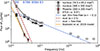 |
Fig. 4. Spectral energy distribution of the Circinus AGN for the three apertures drawn in Fig. 5. Also shown are four ATCA measurements at varying beam sizes (Elmouttie et al. 1998) in white. The dashed lines represent a power-law (Fν ∝ να) fit of the 300 mas nuclear aperture containing both a dust component with α = 3.5 and a free-free component with α = −0.1. We also plot the nuclear dust model by Stalevski et al. (2019) in orange. |
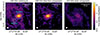 |
Fig. 5. Band 6 (259 GHz) continuum decomposed into a free-free (α = −0.1) and a dust (α = 3.5) component based on pixel-by-pixel SED-fitting. The common beam size between all maps used for these SED fits is drawn in the bottom left as a filled ellipse. In the left figure, we indicate the Phoenix and the two nuclear apertures used to obtain the spectral energy distribution shown in Fig. 4. |
The Phoenix SED resembles a power law that is consistent with pure dust emission (α = [3 − 4] for Fν ∝ να; Hildebrand 1983; Kawamuro et al. 2022). The nucleus shows a power law with a different slope that is consistent with optically thin free-free emission from ionised gas (α = −0.1; Draine 2011). The 300 mas nuclear aperture contains more flux than the central beam, indicating that this free-free component is resolved. We interpret the nuclear emission as free-free radiation rather than synchrotron radiation based on the SED slope and the brightness temperature, which is too low for synchrotron emission (TB ≤ 1.3 × 10³ K; see Sect. B.1 for a discussion on the possible synchrotron contribution from a nuclear jet or the X-ray corona). In B7 and B9, the 300 mas nuclear SED shows a flux density excess compared to the free-free component. As is discussed in T22, this excess is likely caused by thermal emission from cold dust in the equatorial plane surrounding the AGN. This excess cannot be caused by synchrotron radiation from the X-ray corona – as observed in NGC 1068 (Inoue et al. 2020; Mutie et al. 2025) – because we observe no excess at the continuum peak.
To further investigate the morphology of the dust and ionised gas, we decomposed the emission into a dust and a free-free component. We did this for every pixel by performing a least-squares fit that combines two power-law components with α = −0.1 and α = 3.5 for free-free and dust emission, respectively. We plot the equivalent flux density of each component at 259 GHz in Fig. 5. We find that the free-free component traces a nuclear structure that is elongated in the polar direction. The dust component traces a spiral structure similar to that observed in the molecular disc, as well as dust surrounding the AGN in the equatorial direction. From this pixel-based SED decomposition, we find that at 259 GHz, 98% of the flux contained within the 4 × rms contour in Figs. 1 and 6 is free-free emission from nuclear ionised gas.
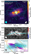 |
Fig. 6. Ionised gas morphology (traced by the 259 GHz continuum) compared to the dusty outflow cone (traced by the mid-IR N-band continuum from Isbell et al. 2022, top panel) and the accretion disc and molecular outflow (traced by the 22 GHz mega-masers from McCallum et al. 2009, middle panel). The B6LB 259 GHz continuum (robust parameter = 0.5) is drawn in the top panel as cyan contours at [4, 8, 16, 32, 64, 128, 256, 512] × rms, with rms = 0.013 mJy/beam. The B6LB and N-band continuum synthesised beam sizes are shown on the bottom left and right, respectively. The middle panel shows the higher resolution (robust parameter = −1) B6LB continuum map with contour levels at [2, 4, 8, 16, 32, 64, 128] × rms, with rms = 0.048 mJy/beam. Overlaid on the middle panel are the 22 GHz maser spots that trace the Keplerian disc (black edge) and the outflow (white edge). The maser spots have a global positional uncertainty of ∼6 mas. The solid cyan lines indicate the fitted outflow trajectories, whereas the dashed cyan lines show these trajectories extrapolated to the maser disc. The orange cross indicates the maser kinematic centre, while the cyan cross indicates the AGN position. The bottom panel shows a schematic representation of the proposed outflow cone geometry. The sketched torus component is based on the B6LB torus morphology in Fig. 3. The grey labels ‘N’ (near) and ‘F’ (far) indicate the respective sides of the warped accretion disc: N marks the near side that is in the line of sight of the AGN, while F corresponds to the far side that is in shadow, as discussed in Sect. 4.2.3. |
The lower resolution ATCA measurements lie near the nuclear α = −0.1 power law when extrapolated from the millimetre (mm) regime towards 1 GHz (as also pointed out by T22). From the inferred electron densities and temperatures (Sect. 4.2), we expect the nuclear free-free emission to become optically thick around ∼3 − 19 GHz (from Eq. 1). Therefore, ATCA measurements contain a significant contribution from nuclear free-free emission but must be dominated by a different emission component at the lowest frequencies (< 3 GHz). This could, for example, be radiation from nuclear star formation (e.g. in the SW ridge; Mueller Sánchez et al. 2006), self-absorbed synchrotron radiation from a weak jet or diffuse synchrotron emission from cosmic-ray electrons (Condon 1992; Mutie et al. 2025). Higher-resolution low-frequency observations are needed to constrain these scenarios.
4.2. Nuclear free-free emission
On sub-parsec to parsec scales, nuclear free-free emission can originate from the compact hot X-ray corona, X-ray heated gas surrounding the accretion disc or from the ionised outflow (Haardt & Maraschi 1991; Palit et al. 2024; Vollmer et al. 2018). The resolved free-free emission on the parsec scale likely traces the ionised outflow because (1) it is orientated along the polar axis, (2) its morphology resembles that of the dust outflow cone, and (3) it is co-spatial with the outflow maser spots (see Fig. 6). The unresolved core, on the other hand, may either be a compact point source (e.g. the X-ray corona) or a disc-like structure, as was observed by Gallimore et al. (2004) in NGC 1068 (component ‘S1’).
The parsec-scale outflow has a brightness temperature of TB ∼ 1 − 40 K at ν = 259 GHz. At this distance from the AGN, we expect the electron temperature to be near the equilibrium photo-ionisation temperature (Wada et al. 2018). We thus assume Te = (0.8−3) × 104 K, which implies an optical depth of τ = −ln[1−(TB/Te)] = (0.33−50) × 10−4. Further assuming a homogeneous electron density, ne, along an optical path of length l = 1 pc, we can estimate ne from (Altenhoff et al. 1960):
 (1)
(1)
which yields ne = (6−46) × 103 cm−3. In the hydrodynamic model of Wada et al. (2018), ionised gas with Te ∼ 104 K and ne ∼ 104 cm−3 is predicted to exist in a wide-angle cone region surrounding the narrow-line region. This electron density is also comparable to the value derived by I23 for the H36α-traced ionised outflow in the Circinus AGN ( ). Assuming Te = 104 K and l = 2 pc as in I23, we find ne = (4.2 − 27)×103 cm−3.
The unresolved core has a much higher antenna temperature4, reaching TA = 1.3 × 10³ K at the highest B6LB resolution (middle panel of Fig. 6). Such a high antenna temperature implies that Te is likely higher than the photo-ionisation temperature because at Te = 104 K, the free-free emission becomes optically thick for ν ≤ 101 GHz, whereas the observed SED slope remains consistent with optically thin emission down to ν = 86 GHz. If, for example, we assume Te ≤ 2 × 10⁴ K, then the implied optical depth at ν = 86 GHz is τ ≥ 0.68, which would reduce the flux density by ≥30% compared to the optically thin case5. No such reduction in flux density is detected at ≥3 σ significance, so this low-temperature scenario is disfavoured. At r < 0.25 pc, strong X-ray heating is instead expected to drive the gas to the Compton equilibrium temperature (Krolik & Begelman 1986). Assuming Te ∼ 6 × 10⁶ K analogous to the S1 region in NGC 1068 (Gallimore et al. 2004) and taking l = 0.25 pc (the beam size), Eq. (1) yields a much higher electron density of ne ∼ 1.3 × 106 cm−3, which is similar to that found by Gallimore et al. (2004) in NGC 1068 (ne ∼ 8 × 105 cm−3). We conclude that the parsec-scale free-free emission and the extended H36α emission trace the ionised outflow at similar density, while the unresolved core represents a distinct, higher-density and temperature component, akin to the S1 region in NGC 1068 (X-ray heated gas in the corona or above the accretion disc).
4.2.1. Ionised outflow
In the top panel of Fig. 6, we compare the parsec-scale outflow traced by the 259 GHz continuum with the dusty outflow cone traced by the mid-IR N-band continuum using the MATISSE interferometer (Isbell et al. 2022). Since the MATISSE measurements lack absolute astrometry, we match the position of the continuum peak in the N-band to the sub-millimetre continuum peak. We find that the N-band morphology is very similar, suggesting that the dusty outflow cone is cospatial with the edge of the ionised outflow cone. Both tracers show a polar extension with a PA of ∼130° and a more compact horizontal bar at PA ∼ 92° surrounding the unresolved continuum peak. We therefore suggest that the clockwise rotation of the contours in our 259 GHz map has the same origin as the horizontal bar in the N-band (Isbell et al. 2022): we predominantly detect one edge of each outflow cone (the W edge of the NW cone and the E edge of the SE cone). Since the emissivity of free-free radiation scales as  (Draine 2011), and given that Te = (0.8 − 3)×104 K, temperature variations alone can account for at most a factor of ∼1.5 in flux density contrast. The observed asymmetry therefore likely reflects a difference in electron density between the two edges of the cone, rather than a temperature difference.
Although the morphology of the N band is essentially point-symmetric6, the extended emission in the B6LB map at r > 1 pc to the north-west is only one-sided. Since the outflow appears point-symmetric in B6SB (Fig. 1 top panel), we conclude that we detect both ionised outflow cones but that the north-western cone is brighter at the parsec scale, making only this cone detectable in the long-baseline map at r > 1 pc. This asymmetry might be the result of slightly denser material in the NW cone. Similarly, I23 detected the ionised outflow as one-sided extended emission towards the north-west in H36α.
In the middle panel of Fig. 6, we compare the B6LB continuum at the highest spatial resolution (14.3 × 12.2 mas2 or 0.29 × 0.24 pc2) with the 22 GHz very long baseline interferometry (VLBI) maser positions of McCallum et al. (2009) (as described in Sect. B.2). At the highest angular resolution, we resolved the horizontal bar into a curved zigzag structure consisting of two linear outer structures with the same orientation as the edge of the dusty outflow cone and an inner unresolved core. We find that the outflow masers extend farther outwards from the polar axis (and closer to the mid-plane) than the 259 GHz and N-band continuum at the northern (southern) side of the eastern (western) outflow edge. This implies a stratification between the ionised outflow and the outflowing maser clumps (blue and purple cones in Fig. 6), with the molecular outflow having a slightly wider opening angle.
4.2.2. Launching or collimation radius
The curved zigzag morphology of the 259 GHz continuum indicates that we resolved the base of the ionised outflow cone for the first time in the Circinus AGN. If we assume that the outflowing material follows straight trajectories after leaving the disc, we can estimate the radius of the base as follows. We fit two straight lines to the outer linear structures (solid cyan lines in Fig. 6) and then extrapolate these trajectories inwards to the maser disc (dashed cyan lines in Fig. 6). We find that they connect to the disc at the edges of the inner warped maser disc section at r ≈ 0.16 pc with half-opening angles of θW ≈ 44° and θE ≈ 29° for the western and eastern trajectories, respectively7. We can interpret this radius in two ways: either as a launching radius or as a collimation radius.
It has previously been suggested that the collimation of AGN outflows is caused by the torus or by a warped accretion disc (Fischer et al. 2013). Since the outer sections of the maser disc (red and blue lines in the bottom panel of Fig. 6) coincide with the edges of the ionisation cones, we suggest that the warped maser disc collimates the ionised outflow before the outflow reaches the torus. This cannot be concluded for the ‘outflow masers’, which trace a cone that is wider than the warped maser disc. This is consistent with the molecular outflow being instead collimated by the torus or these maser clumps tracing molecular torus material that is shocked by the outflow. If the observed geometry is indeed the result of collimation, any mechanism with a launching radius r < 0.16 pc is consistent with our observations.
An alternative interpretation is that we directly observe the launching radius. In the radiation-driven mechanism proposed by Hönig & Kishimoto (2017), the ionised and dusty wind is launched near the dust sublimation radius, which is equal to rsub = 0.05 − 0.2 pc for Circinus (depending on the dust composition and AGN luminosity; Isbell et al. 2023). Our observations are therefore consistent with the outflow mechanism proposed by Hönig & Kishimoto (2017). The assumption of rlaunch = 0.16 pc in Andonie et al. (2022) is also consistent with our result, while rlaunch = 0.53 pc in Vollmer et al. (2018) appears too large.
4.2.3. Anisotropic launching mechanism
In the mid-IR, the asymmetry observed between the edges of the dusty outflow cones has previously been attributed to anisotropic illumination by a tilted inner accretion disc (Tristram et al. 2014), with the W and E edges appearing hotter than the N and S edges due to preferential exposure to the central radiation source (see also Stalevski et al. 2017, 2019). However, our observations suggest a difference in density, rather than temperature, between both edges of the ionisation cone.
This leads us to propose the following explanation. The continuum morphology at 259 GHz shows that the outflow trajectories (cyan lines in Fig. 6) intersect regions located ∼0.1 pc above the outer parts of the warped maser disc. The material located on these near sides of the maser disc (labelled ‘N’ in the bottom panel of Fig. 6) lies in direct sight of the AGN. This material can therefore be efficiently launched either by radiation pressure from the inner accretion disc or entrainment in a wide-angle wind that originates close to the AGN. In contrast, material on the far sides of the maser disc (labelled ’F’) is shielded by the warped optically thick accretion disc. We therefore suggest that we detect an anisotropic wind launching from a warped disc rather than an anisotropic illumination of an otherwise isotropic wind. Unlike the model of Stalevski et al. (2017), our interpretation does not require a tilt of 40° of the inner accretion disc relative to the polar axis within the inner region.
4.3. Nuclear dust emission
To the south-east of the nucleus, we detect the Phoenix feature. Its emission, which extends out in the radial direction to a projected distance of ∼8 pc from the nucleus, is associated with dust as is shown in Sect. 4.1. The phoenix ends in a flux enhancement, where it splits into two ‘wings’. When comparing the morphology of the Phoenix with that of the molecular spiral arms, as is shown in Fig. 7, we find that they trace very different structures. The molecular maps show no structure extending radially outwards from the AGN, and the eastern ridge in the CND does not coincide with the ridge created by the two wings of the Phoenix. We discuss two possible scenarios in the following subsections.
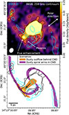 |
Fig. 7. Top panel: Phoenix feature as observed in the B6SB 259 GHz continuum compared to the B7 CO(3-2) molecular tracer (blue contour at 1.0 mJy/beam km/s). We observe a mismatch between the continuum and CO(3-2) morphology, which either implies that the Phoenix feature is associated with a polar outflow perpendicular to the CND or that the inner spiral arm structure traced by dust differs from the molecular spirals. Bottom panel: Illustration of both of these scenarios. The spiral pattern drawn in purple is based on the structure observed in the right panel of Fig. 5. The B6SB 259 GHz continuum contours are drawn at [6, 8] × rms, with rms = 0.022 mJy/beam. |
4.3.1. Outflow scenario
Because of the morphological discrepancy and the polar orientation, we suggest that the Phoenix might not be part of the CND but is instead located behind the disc as part of a dusty outflow (as illustrated in Fig. 7). This dust would not be shielded by the torus, so we expect it to be warmer than the dust in the mid-plane.
At the kiloparsec scale, Elmouttie et al. (1998) discovered a bipolar outflow in the 20 cm radio continuum. The PA of the Phoenix feature (≈135°) differs slightly from that of the SE kiloparsec-scale outflow (≈115°), but it is nearly perpendicular to the PA of the inner tilted maser disc (≈48°) from which it would be launched. It is also almost exactly opposite the direction of the collimated ionised outflow on the NW side (≈320°; Kakkad et al. 2023). Therefore, the Phoenix would be the SE counterpart of the NW outflow. The ∼40 pc-scale warm dust component observed in the mid-IR by Stalevski et al. (2017) has a significantly different PA of ≈100°, meaning that it would have to trace a different (temperature) component than the Phoenix.
The fact that the Phoenix abruptly ends in a flux enhancement and splits into two perpendicular wings could imply that the material slows down and eventually falls back to the disc. This would mean that we would directly detect the dust fountain as proposed by Wada et al. (2016). Such a backflow of dust and gas would add to the turbulent motion in the disc, which is one proposed mechanism to keep the torus geometrically thick. The flux enhancement could then be associated with a collision of the outstreaming column of material onto a dense clump, causing a build-up of material or heating of the dust. A very similar picture of a collimated outflow splitting into two branches due to a dense clump was presented by Kakkad et al. (2023) on the NW side of the Circinus AGN (referred to as the ‘tuning fork’) to explain the morphology in the [O III] cone.
4.3.2. Spiral arm scenario
Another explanation for the mismatch in morphology is that the dusty and molecular arms are simply not cospatial. This offset between dust and molecular gas has been observed at the kiloparsec scale in several spiral galaxies, where this offset results from warm dust that is heated by star formation triggered in the density wave (Patrikeev et al. 2006; Chandar et al. 2017; Vallée 2020). Because a similar offset is also observed to the NW of the CND between the spiral dust arm and the NW molecular hook, a similar offset at the SE side of the CND would be plausible.
4.4. CND kinematics
The material surrounding molecular tori is hypothesised to contain non-circular motions responsible for inflows and outflows, for example, as part of the fountain model introduced by Wada et al. (2016). We are therefore interested in the kinematics of the molecular gas in the Circinus CND. In particular, the spiral structure observed in the CND could induce non-circular motions in the material orbiting the SMBH (Roberts et al. 1979; van de Ven & Fathi 2010). Moment-one maps of the B6SB HCO+(3-2) and HCN(3-2) emission are presented in the left panels of Fig. 8. We find a strong dipole that indicates that the kinematics is dominated by rotation. However, on the basis of the velocity contours, we find that the observed velocity field is not symmetric around the minor and major rotation axes of this dipole. The CND must therefore contain gas motions that deviate significantly from a pure circular rotation around a single rotation axis.
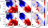 |
Fig. 8. Velocity fields of the CND for HCO+(3-2) (top) and HCN(3-2) (bottom) from the B6SB dataset as observed (left), as modelled using 3DBAROLO (middle) and the residual velocity field that results from subtracting the model from the data (right). The black arrows in the right panels indicate the position of the blue residual feature that coincides with the position of the NW hook. Velocity contour levels are drawn at [ − 75, −50, −25, 0, 25, 50, 75] km s−1. The rest frame velocity is defined relative to Vsys = 441.4 km s−1. Indicated on all maps are the point apertures used to extract the 1D kinematic profiles shown in Fig. 10 using corresponding symbols in white. The synthesised beam sizes are drawn in the bottom left as filled ellipses, and the cyan cross indicates the AGN position. |
To determine whether the observed asymmetry arises from non-circular gas movements or a warp in the disc position angle (PA), we modelled the HCO+(3–2) and HCN(3–2) kinematics using the software 3DBAROLO (Di Teodoro & Fraternali 2015), which fits 3D tilted ring models directly to emission line data cubes. Initially, we only allowed circular motion in the 3DBAROLO model such that any non-circular motion can be investigated from the residual velocity field after subtracting the model from the observed velocity field. We defined 29 tilted concentric rings placed at regular intervals between r = 0.05″ and r = 1.45″ centred on the AGN position. For each ring, we fitted the rotation velocity, Vrot, the dispersion velocity within the disc, Vdisp, the inclination angle, i, the position angle of the major axis on the receding side, PA, and the systemic velocity, Vsys, using χ2 minimisation. We used a pixel-by-pixel normalisation of the surface density, which allowed the model to reproduce the clearly non-symmetric intensity distribution in the Circinus CND. The fitting process was executed in two stages. In the first stage, all free parameters were unconstrained and were fitted to each ring separately. In the second stage, the inclination and position angles were regularised through a radial Bezier function, and the systemic velocity was fixed at the median value of all rings. In addition, we performed an alternative fit in which the radial velocity, Vrad, is included as a free parameter in the model. We discuss this additional fit in Sect. C.3.
The resulting radial parameter profiles are shown in Fig. 9, and the resulting moment-one model and residual velocity fields are shown in Fig. 8. We discuss the major-axis position-velocity (PV) diagram of both the model and the data in Sect. C.1. In general, we find that the fitted parameters and the residual velocity fields are robust against changes in initial parameters. We also find that HCO+(3-2) and HCN(3-2), within the statistical uncertainties, trace the same circular rotation structure in the disc. The systemic velocities are fitted to be 441.9 ± 0.9 km s−1 and 440.8 ± 0.9 km s−1 for the HCO+(3-2) and HCN(3-2) transitions, respectively. We therefore conclude that the average fitted systemic velocity of the CND is equal to Vsys = 441.4 ± 0.7 km s−1, which is consistent with the nominal systemic velocity of 439 ± 2 km s−1 of the galaxy and the nuclear molecular material (Freeman et al. 1977; Curran et al. 1998). We find Vdisp to range between ≈10 km s−1 and ≈23 km s−1 throughout the disc, and the inclination angle and position angle are i = 75 ± 3° and PA = 218 ± 6°. These results are consistent with the kinematic analysis from T22, but have smaller uncertainties.
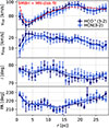 |
Fig. 9. Fitted kinematic and morphological radial parameters of the CND from 3DBAROLO modelling of the HCO+(3-2) and HCN(3-2) transitions in the B6SB dataset. The top two panels show the 3DBAROLO fitting results and the associated uncertainties after the second fitting iteration, while the bottom two panels show the fit results and uncertainties from the first iteration as scatter points with the regularised radial parameter profiles overlaid as solid curves that are used in the second iteration. The SMBH + Miyamoto-Nagai disc rotation curve fit is overlaid in the top panel as a red dashed line. |
The rise in the rotation curve for r < 3 pc (see Fig. 9) indicates a mass concentration near the disc centre. Although the interpretation of these results warrants caution for the inner two rings (since the minor axis is unresolved, as is discussed in Sect. C.1), the observed increase in Vrot and the drop in Vdisp at r < 3 pc are consistent with the higher resolution modelling by I23. Except for the innermost ring, all fitted line-of-sight velocities are higher than would be expected from the Keplerian profile of a M• = (1.7±0.3) × 106 M⊙ SMBH (see Fig. C.1; Greenhill et al. 2003). Approximating with spherical symmetry, the dynamical mass enclosed within radius r is given by: M(r) = rVrot(r)2/G, with G the gravitational constant. Using the fitted rotational velocity of Vrot ≈ 70 km s−1 at r = 2 pc (which encloses the torus structure), we find a dynamical mass of ≈2.6 × 10⁶ M⊙. This implies a dynamical torus mass of ∼9 × 10⁵ M⊙ after subtraction of the SMBH mass8. At larger radii, the rotational velocity increases to ∼90 km s−1 out to a radius of 17 pc, implying that the CND kinematics is dominated by self-gravitation. We model this rotation curve using a 1.7 × 10⁶ M⊙ point mass surrounded by a Miyamoto-Nagai (MN) disc (Miyamoto & Nagai 1975), for which we assume a scale height9 of b/a = 0.22 (with a and b the length and thickness scales of the MN disc) and fit a disc scale length of a = 13.3 ± 0.5 pc and an enclosed disc mass of MMN(r ≤ 28 pc)≡MCND = (3.2±0.2) × 107 M⊙ (see Fig. 9).
Looking at the residuals in the velocity fields (right panels in Fig. 8), we find that large residuals remain after subtraction of the model. This is a clear indication of non-circular motions. The blue residual to the north-west of the SMBH (indicated with a black arrow in Fig. 8) is the strongest and has a magnitude of ∼ − 40 km s−1. In addition, we observe a significant redshift residual in a more extended region to the south-east of the SMBH with a magnitude of ∼20 km s−1. As is discussed in Sect. C.2, these residuals are not caused by improper modelling (e.g. due to the PA being significantly larger in the inner disc than assumed by the model). In Fig. 10, we show four 1D kinematic profiles that we extracted from the point apertures indicated in Fig. 8. We find that the blue and red residuals in the northern and southern apertures are not caused by a secondary blue or red shifted velocity component. Instead, we find that all apertures show an approximately Gaussian profile that is similar to the model but shifted to a different velocity. Therefore, these residuals are the result of motions within the disc itself and not due to an additional molecular outflow that is launched from the disc or material falling back onto the disc.
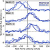 |
Fig. 10. Kinematic 1D profiles of HCO+(3-2) and HCN(3-2) in B6SB extracted from the four point apertures as indicated in Fig. 8 using corresponding markers. We show the data as a step curve and the 3DBAROLO model as dashed curves. The 1D kinematic profiles are normalised by the maximal flux density in the model. The spectra are offset by a term c as indicated by the horizontal dotted lines. |
4.5. Torus feeding through inflow in the CND
The blueshifted emission in the residual maps of Fig. 8, located north-west of the SMBH, originates, at least for the most part, from the structure we identified as the NW hook. This is because in the HCO+(3-2) and HCN(3-2) maps of B6SB, on which the kinematic modelling is based, the blue residual spatially coincides with the NW-arm (cyan contours in Fig. 3). Further confirmation comes from overlaying the blue residual onto the higher-resolution band 7 maps in Figure A.2, where the blue residual again coincides with the NW hook.
Since the NW hook is located on the far side of the CND, we interpret this blueshift as an inflow along the NW hook. We interpret this as an inflow rather than an outflow because (a) the corresponding 1D kinematic profile only shows one blueshifted velocity component from the disc rather than a disc component and an extra blueshifted outflow component (b) the blueshifted emission originates from a structure that morphologically resembles a spiral arm, which would be associated with instabilities within the self-gravitating gaseous disc and (c) the position angle and location of the known outflow, which is tilted towards the west side of the rotation axis (see Figs. 1, 5, 6 and the dusty and ionised outflow as traced by Stalevski et al. 2017; Isbell et al. 2022; Kakkad et al. 2023 and I23), do not match with the position of the blue residual, which is located to the north-east of the rotation axis. Therefore, we conclude that gas is transported inwards along the NW hook, which connects to the approaching side of the torus, thereby feeding the torus.
Following the same logic as for the NW hook, the redshifted feature on the near side of the CND would also be associated with an inflow. Based on the morphology of the residual velocity map, this inflow would be less collimated and smaller in magnitude (∼20 km s−1). Since this redshifted region coincides with the location of the E ridge and the SW hook, these southern spiral structures could be responsible for the angular momentum transfer required for the inward transport of material on this side of the disc. However, in contrast to the inflow motion observed to the NW, this inward motion would be perpendicular to the E ridge rather than along the length of the spiral arm. At the location where the SW hook connects to the torus, we observe no significant velocity residual. This does not imply that there is no inward transport of material on this side of the torus because we are insensitive to a radial inflow at this location (which would be perpendicular to our line of sight).
As an extra check that the observed residuals imply inflow, we performed a second 3DBAROLO fit where we allow the rings to have non-zero axisymmetric radial velocities (see Sect. C.3). We find that the model consistently predicts an inflow in the central region of the CND (r < 15 pc) that increases in velocity towards the SMBH, with a mean magnitude of Vrad ∼ −12 km s−1 between 5 pc and 15 pc (see Fig. C.2). The resulting residuals on the velocity map are similar in shape but have a smaller magnitude than those of the model that fixes Vrad = 0 km s−1 (Fig. C.3). This is not surprising, since we measured a projected inflow velocity of ≈40 km s−1 in the NW hook, which is much faster than the inflow in the axisymmetric inflow model. We therefore conclude that the inflow is not axisymmetric and is dominated by the motions in or near the spiral arms.
Nuclear spirals are known to exist on > 10 pc scales in AGN-bearing galaxies. These are often connected to the CND10 and thought to be responsible for AGN feeding based on the non-axisymmetric potential that they produce (see e.g. Pogge & Martini 2002; Prieto et al. 2005; Combes et al. 2014; Audibert et al. 2019; Combes et al. 2019; Storchi-Bergmann & Schnorr-Müller 2019). Our observations of the Circinus nucleus reveal a case where we observe a clear spiral structure within the CND that connects to a kinematically distinct sub-structure (the torus) and transports material down to the parsec-scale torus. Such a spiral structure in the Circinus CND is not unexpected, since the Toomre-Q parameter is smaller than unity outside r = 1 pc (Toomre 1964; I23), meaning that we expect gravitational instabilities to grow into spiral structures. These bars and spirals then produce negative torques that drive inflow (Buta & Combes 1996; Combes 2021a).
4.5.1. Torus feeding rate
The feeding rate of the torus through the NW hook can be estimated by multiplying the radial inflow velocity by the linear gas mass density in the inner straight bar of the hook. Since the stars in the CND are collisionless, their motion is expected to be decoupled from that of the gas (Schnorr Müller et al. 2011; Schartmann et al. 2017). We thus assume that only the gas contributes to the inflow rate. Because the disc is tilted by i = 76 ± 1° at the point aperture in the NW hook (square marker in Fig. 8), it intersects the CND at a de-projected distance of r = 14 pc. At this aperture, we measure a residual velocity of VLOS, NW = −39 ± 2 km s−1. Assuming that the residual gas motion is purely radial after subtraction of the fitted rotational velocity component, we find a de-projected radial velocity of Vrad, NW = VLOS/(sin i×cos ϕ) = −43 ± 2 km s−1. Here, ϕ = 23° is the angle between the inner bar of the NW hook and the disc minor axis.
It is difficult to determine the gas mass enclosed in the NW hook from the line intensities. This is because, assuming a gas fraction of fgas ∼ 0.5 (Mueller Sánchez et al. 2006; Hicks et al. 2009), the Miyamoto-Nagai disc model predicts a mean face-on column density of NH2 = 4.8 × 1023 cm−2 at r = 14 pc, which makes all observed transitions optically thick11. We therefore have to rely on more rudimentary estimates. Since the width of the SW hook is partially resolved in B7 (see Fig. A.2), we assume a diameter of D ∼ 1 pc for the NW hook, comparable to the B7 beam size. Approximating its shape as a cuboid of side length D = 1 pc, elongated radially along the inner straight bar, and filled with gas at a mean density of nH2 ∼ ncrit, HCO+(3 − 2) = 106 cm−3, we find an inflow rate of
 (2)
(2)
where mH2 = 3.35 × 10⁻²⁷ kg is the mass of a hydrogen molecule. In this toy model, the NW hook has a face-on column density of NH2 = nH2 × D = 3.1 × 1024 cm−2. If we instead set NH2 = 4.8 × 1023 cm−2 equal to the mean column density of the Miyamoto-Nagai disc at r = 14 pc (implying nH2 = 1.5 × 105 cm−3), we find an inflow rate of ṀNW-hook ∼ 0.3 M⊙ yr−1. We can treat this latter value as a lower limit because the gas density in the NW hook is likely higher than the average density throughout the CND.
To determine the total feeding rate of the torus, we also have to consider the mass inflow through the rest of the disc. Since an inflow along the SW hook would be perpendicular to our line of sight, we cannot perform an analogous calculation of ṀSW-hook. However, based on the second 3DBAROLO fit, where Vrad was left as a free parameter to describe the axisymmetric radial velocities in the rings, we can calculate an inflow rate for the entire disc (for details, see Appendix C.4). The resulting radial inflow profile (bottom panel Fig. C.2) is constant at Ṁinflow = 7.5 ± 1.5 M⊙ yr−1 between r = 3 pc and r = 14 pc. As is discussed in Appendix C.4, we expect this total inflow rate to be an overestimate. We therefore constrain the torus feeding rate to Ṁfeed = 0.3−7.5 M⊙ yr−1.
These feeding rates are higher than those reported by I23 for the Circinus AGN, who derived Ṁfeed = 0.20−0.35 M⊙ yr−1 from the redshifted absorption profile described in Sect. 3.2. Our estimates are likely more robust, as Baba et al. (2024) showed that infalling clumps traced by absorption do not necessarily provide a reliable measure for the total mass inflow rate. Furthermore, I23 used rinflow = 0.27 pc in their calculation, whereas Baba et al. (2024) showed that such absorption signatures are more likely to originate at much larger radii in the CND. Our inferred feeding rate also exceeds that obtained in the hydrodynamic simulation by Baba et al. (2024), which yielded a maximum of Ṁfeed ∼ 0.35 at r = 5 pc.
4.5.2. Mass flow and feeding timescales
The Eddington accretion rate of the Circinus AGN is equal to  (for a radiative efficiency of η = 0.1 and an Eddington luminosity of
  , Tristram et al. 2007), which is only 12% of our lower torus feeding limit. This implies that the majority (> 88%) of the incoming mass must be removed from the AGN before reaching the accretion disc and must be expelled to distances beyond r ∼ 14 pc as part of an outflow. Estimates for the ionised and molecular outflows range between Ṁout,ion = 0.01−0.22 M⊙ yr−1 (Fonseca-Faria et al. 2021; Kakkad et al. 2023; I23) and Ṁout,mol = 0.35−12.3 M⊙ yr−1 (Zschaechner et al. 2016), respectively. Our values for the torus feeding rate are thus consistent with those required to sustain accretion and outflow. Although part of the inflow is used for star formation, this is a small fraction of the total mass flow since Esquej et al. (2013) reported a rate of only ṀSFR = 0.13 M⊙ yr−1 within 75 pc of the AGN.
Since we estimated dynamical masses of Mtorus ∼ 9 × 10⁵ M⊙ and MCND = (3.2±0.2) × 107 M⊙, the implied timescales are tfeed, torus = 120 kyr − 2.7 Myr and tdepl, CND = 4.3 − 97 Myr. Assuming a steady state with approximately Ṁfeed ≈ Ṁacc + Ṁoutflow = Ṁdepl, we also expect tdepl, torus ∼ tfeed, torus. Since both the torus and the CND act as mass reservoirs for the AGN, any variation in the activity of the AGN caused by inhomogeneities in the CND would be expected on timescales of ∼tdepl, CND and would be time-smoothed on timescales larger than tdepl, torus. These timescales are similar to those observed for the (de)activation of AGNs, both based on fluctuations in multi-phase outflows (e.g. ∼3 Myr in the Fornax A galaxy, Maccagni et al. 2021) and on radio jets, which typically show AGN activity cycles lasting 1 − 100 Myr (Parma et al. 1999; Brienza et al. 2017; Combes 2021a). This suggests that such fluctuations in AGNs may be directly related to the variability in torus feeding by the CND.
5. Conclusions
In this work, we have used high-resolution (down to 13 mas or 0.25 pc) ALMA observations of the Circinus AGN to investigate the feeding of the molecular torus and the launching of the ionised outflow. We focused on the CND (size ∼50 pc), the torus (size ∼2.4 pc), and the AGN outflows at the parsec scale. We investigated the emission mechanisms and morphology of the continuum radiation between 86 GHz and 665 GHz and studied the morphology and kinematics of the molecular gas using the HCO+(3-2), HCO+(4-3), HCN(3-2), HCN(4-3), and CO(3-2) emission lines. We summarise our findings as follows.
-
At 1 pc ≲ r ≲ 28 pc distance from the nucleus, the millimetre continuum traces thermal emission from cold dust located in the equatorial mid-plane of the CND and the torus. The cold dust in the CND is distributed in two spiral arms. Towards the SE from the nucleus, we detect the Phoenix feature, which we interpret either as warm dust in an outflowing dust fountain or as cold dust in a spiral structure that is offset from the molecular gas spirals in the CND.
-
At the parsec scale, the nuclear millimetre continuum traces optically thin free-free radiation from the ionised outflow. We derive electron densities of the order of ne ∼ 104 cm−3 for Te ∼ 104 K. The ionised outflow cone morphology matches that of the dusty outflow cone but differs from the morphology of the molecular outflow, suggesting a stratification between the molecular outflow (wider opening angle) and the dusty and ionised outflow (smaller opening angle).
-
The millimetre continuum shows an unresolved (≲0.25 pc) central emission peak. We interpret this as optically thin free-free emission from X-ray heated gas in the corona or above the maser disc with ne ∼ 1.3 × 106 cm−3 for Te ∼ 6 × 10⁶ K. We do not detect synchrotron emission from a jet or the corona.
-
We measured the base of the ionised outflow to have a radius of r ≈ 0.16 pc – which is either a collimation or a launching radius – and determined half-opening launch angles of θW ≈ 44° and θE ≈ 29°. We found evidence that the ionised outflow is collimated by the warped accretion disc and that the ionisation cones appear asymmetric due to an anisotropic launching mechanism (rather than anisotropic illumination).
-
The molecular line emission reveals spiral arms in the CND that consist of four distinct sub-structures and differ in position from the dusty spirals. Two of these structures, the NW hook and the SW hook, connect to the torus.
-
We find that the kinematics of the CND is dominated by rotation due to self-gravitation with dynamical masses of MCND = (3.2±0.2) × 107 M⊙ and Mtorus ∼ 9 × 10⁵ M⊙. In addition, we observe non-circular inward motion of the order of 20 − 40 km s−1 that is concentrated in the spiral structure.
-
These inward gas flows suggest that the non-axisymmetric potential generated by the spiral arms is responsible for driving the inflow from the CND down to the parsec-scale torus.
-
We determined the torus feeding rate to be Ṁfeed = 0.3−7.5 M⊙ yr−1, which implies that > 88% of the material that flows towards the torus is expelled in outflows before it reaches the inner accretion disc. These rates imply characteristic feeding timescales of tfeed, torus = 120 kyr − 2.7 Myr and tdepl, CND = 4.3 − 97 Myr, which suggests that the fluctuations in AGN activity often observed on such timescales may be caused by variability in the torus feeding rate.
In summary, we report the first resolved detection of the ionised outflow base in Circinus, unveiling important details about the launching mechanism, and we provide the most detailed kinematic evidence to date for torus feeding at parsec scales through spiral arms that are embedded in the CND. Observations at a similar spatial resolution of other AGNs will be required to confirm if these mechanisms are universal or specific to the Circinus AGN, and higher-resolution observations in the inner parsec of the Circinus nucleus are needed to constrain the launching mechanism.
Data availability
The continuum and molecular moment zero maps presented in Figs. 1, 2, 3 and A.2 as well as an extended version of Table A.2 are available at the CDS via https://cdsarc.cds.unistra.fr/viz-bin/cat/J/A+A/704/A125
We use sidelobethreshold = 3.0, noisethreshold = 5.0, minbeamfrac = 0.3 and lownoisethreshold = 2.0. For continuum imaging, we set negativethreshold = 0.0 and used the Hogbom algorithm. For line imaging, we instead used negativethreshold = 7.0 and multi-scale cleaning.
We name this structure the Phoenix since this protrusion ends in a flux enhancement that resembles a head. At this head, the structure splits into two ‘wings’.
Based on the Einstein A coefficients and collisional rates from the Leiden Atomic and Molecular Database (LAMBDA; Schöier et al. 2005; Yang et al. 2010).
TB represents the intrinsic surface brightness, while TA is the measured surface brightness. In general, TB ≥ TA due to beam dilution.
In the optically thin case, 60% of the flux density in the 86 GHz common beam would correspond to the B6LB unresolved core and 40% to the ionised outflow. The total attenuation thus equals 0.6 × (1−e−τ).
We ascribe the lack of asymmetry in the N-band map from Isbell et al. (2022) to a bias towards point symmetry in the MATISSE imaging since Tristram et al. (2014) found polar asymmetry in the N-band.
As measured from the polar axis, which we assume to be perpendicular to the inner section of the maser disc.
We ignore the mass of the accretion disc, on which Greenhill et al. (2003) placed an upper limit of Macc ≲ 4 × 10⁵ M⊙ within r = 0.4 pc.
Since Vdisp/Vrot ≈ 0.22. We follow the method from Krolik & Begelman 1988, which states that b/a ∼ Vdisp/Vrot in the torus disc. If we, for example, instead choose b/a = 0.1, MCND is reduced by 7%.
In some cases, such as Combes et al. (2019), this disc is referred to as the torus, where it is uncertain if this structure is what obscures the AGN. By that definition, the disc we refer to as the CND could be called the torus, implying that we observe spiral structure within the torus.
Using RADEX (van der Tak et al. 2007), we find τ ≫ 1 for Tgas ≤ 50 K, line widths of 50 km s−1, nH2 = ncrit for each transition and chemical abundances of XCO ∼ 10−4 and XHCN ∼ XHCO+ ∼ 3 × 10⁻⁹ (Viti et al. 2014; Szűcs et al. 2016; Gámez Rosas et al. 2025).
The antenna temperature is equal to the brightness temperature only if a source is resolved.
We note that the inner rings are not relevant for the fitting of the Miyamoto-Nagai model since we fixed the mass of the SMBH, which is the dominant source of gravity at these radii.
Acknowledgments
The authors thank B. Vollmer, C. Ricci, A. Pizzetti, S. Viti, J.W. Isbell, Y. Zhang, J.F. Gallimore, J.J. Butterworth, P.P. van der Werf, F. Fraternali, P.E. Mancera Piña, H.J.A. Röttgering, C.A. Vleugels, N.N. Geesink, R.S. Dullaart, F.J. Ballieux, A. Krämer, W.C. Schrier, B. Goesaert, V. Baeten & D.J. Remmelts for their advice and many helpful discussions. We also thank the anonymous reviewer for the thorough report, which significantly improved the quality of this paper. W.M. Goesaert acknowledges support from ESO and the Leiden University Fund. This paper makes use of the following ALMA data: 2018.1.00581.S, 2017.1.00575.S and 2019.1.00013.S. ALMA is a partnership of ESO (representing its member states), NSF (USA) and NINS (Japan), together with NRC (Canada), MOST and ASIAA (Taiwan), and KASI (Republic of Korea), in cooperation with the Republic of Chile. The Joint ALMA Observatory is operated by ESO, AUI/NRAO and NAOJ.
References
- Altenhoff, W., Mezger, P. G., Wendker, H., & Westerhout, G. 1960, Veröffentlichungen der Univer-sitäts-Sternwarte zu Bonn, 59, 48 [Google Scholar]
- Andonie, C., Ricci, C., Paltani, S., et al. 2022, MNRAS, 511, 5768 [NASA ADS] [CrossRef] [Google Scholar]
- Andreani, P., Carpenter, J., Trigo, M. D., et al. 2018, ALMA Cycle 6 Proposer’s Guide, ALMA Doc. 6.2 v1.0 [Google Scholar]
- Antonucci, R. 1993, ARA&A, 31, 473 [Google Scholar]
- Audibert, A., Combes, F., García-Burillo, S., et al. 2019, A&A, 632, A33 [NASA ADS] [CrossRef] [EDP Sciences] [Google Scholar]
- Baba, S., Wada, K., Izumi, T., Kudoh, Y., & Matsumoto, K. 2024, ApJ, 966, 15 [Google Scholar]
- Beckmann, V., Gehrels, N., Shrader, C. R., & Soldi, S. 2006, ApJ, 638, 642 [NASA ADS] [CrossRef] [Google Scholar]
- Blundell, K. M., & Kuncic, Z. 2007, ApJ, 668, L103 [NASA ADS] [CrossRef] [Google Scholar]
- Brienza, M., Godfrey, L., Morganti, R., et al. 2017, A&A, 606, A98 [NASA ADS] [CrossRef] [EDP Sciences] [Google Scholar]
- Buta, R., & Combes, F. 1996, Fund. Cosmic Phys., 17, 95 [Google Scholar]
- Chan, C.-H., & Krolik, J. H. 2016, ApJ, 825, 67 [NASA ADS] [CrossRef] [Google Scholar]
- Chandar, R., Chien, L.-H., Meidt, S., et al. 2017, ApJ, 845, 78 [NASA ADS] [CrossRef] [Google Scholar]
- Combes, F. 2021a, Active Galactic Nuclei: Fueling and Feedback (Bristol: IOP Publishing) [Google Scholar]
- Combes, F. 2021b, in Galaxy Evolution and Feedback across Different Environments, eds. T. Storchi Bergmann, W. Forman, R. Overzier, & R. Riffel, IAU Symp., 359, 312 [NASA ADS] [Google Scholar]
- Combes, F., García-Burillo, S., Casasola, V., et al. 2014, A&A, 565, A97 [NASA ADS] [CrossRef] [EDP Sciences] [Google Scholar]
- Combes, F., García-Burillo, S., Audibert, A., et al. 2019, A&A, 623, A79 [NASA ADS] [CrossRef] [EDP Sciences] [Google Scholar]
- Comrie, A., Wang, K. S., Hsu, S. C., et al. 2018, CARTA: The Cube Analysis and Rendering Tool for Astronomy (Zenodo) [Google Scholar]
- Condon, J. J. 1992, ARA&A, 30, 575 [Google Scholar]
- Curran, S. J., Johansson, L. E. B., Rydbeck, G., & Booth, R. S. 1998, A&A, 338, 863 [NASA ADS] [Google Scholar]
- Di Teodoro, E. M., & Fraternali, F. 2015, MNRAS, 451, 3021 [Google Scholar]
- Dorodnitsyn, A., Bisnovatyi-Kogan, G. S., & Kallman, T. 2011, ApJ, 741, 29 [Google Scholar]
- Draine, B. T. 2011, Physics of the Interstellar and Intergalactic Medium (Princeton University Press) [Google Scholar]
- Elmouttie, M., Haynes, R. F., Jones, K. L., Sadler, E. M., & Ehle, M. 1998, MNRAS, 297, 1202 [Google Scholar]
- Emmering, R. T., Blandford, R. D., & Shlosman, I. 1992, ApJ, 385, 460 [NASA ADS] [CrossRef] [Google Scholar]
- Esquej, P., Alonso-Herrero, A., González-Martín, O., et al. 2013, ApJ, 780, 86 [Google Scholar]
- Fischer, T. C., Crenshaw, D. M., Kraemer, S. B., & Schmitt, H. R. 2013, ApJS, 209, 1 [Google Scholar]
- Fonseca-Faria, M. A., Rodríguez-Ardila, A., Contini, M., & Reynaldi, V. 2021, MNRAS, 506, 3831 [CrossRef] [Google Scholar]
- Freeman, K. C., Karlsson, B., Lynga, G., et al. 1977, A&A, 55, 445 [NASA ADS] [Google Scholar]
- Gallimore, J. F., Baum, S. A., & O’Dea, C. P. 2004, ApJ, 613, 794 [Google Scholar]
- Gámez Rosas, V., van der Werf, P., Gallimore, J. F., et al. 2025, A&A, 699, A187 [NASA ADS] [CrossRef] [EDP Sciences] [Google Scholar]
- García-Burillo, S., Combes, F., Ramos Almeida, C., et al. 2016, ApJ, 823, L12 [Google Scholar]
- Greenhill, L. J., Booth, R. S., Ellingsen, S. P., et al. 2003, ApJ, 590, 162 [NASA ADS] [CrossRef] [Google Scholar]
- Haardt, F., & Maraschi, L. 1991, ApJ, 380, L51 [Google Scholar]
- Harrison, C. M., & Ramos Almeida, C. 2024, Galaxies, 12, 17 [NASA ADS] [CrossRef] [Google Scholar]
- Hicks, E. K. S., Davies, R. I., Malkan, M. A., et al. 2009, ApJ, 696, 448 [NASA ADS] [CrossRef] [Google Scholar]
- Hildebrand, R. H. 1983, QJRAS, 24, 267 [NASA ADS] [Google Scholar]
- Hönig, S. F., & Kishimoto, M. 2017, ApJ, 838, L20 [Google Scholar]
- Impellizzeri, C. M. V., Gallimore, J. F., Baum, S. A., et al. 2019, ApJ, 884, L28 [NASA ADS] [CrossRef] [Google Scholar]
- Inoue, Y., Khangulyan, D., & Doi, A. 2020, ApJ, 891, L33 [Google Scholar]
- Isbell, J. W., Meisenheimer, K., Pott, J. U., et al. 2022, A&A, 663, A35 [NASA ADS] [CrossRef] [EDP Sciences] [Google Scholar]
- Isbell, J. W., Pott, J. U., Meisenheimer, K., et al. 2023, A&A, 678, A136 [NASA ADS] [CrossRef] [EDP Sciences] [Google Scholar]
- Izumi, T., Wada, K., Fukushige, R., Hamamura, S., & Kohno, K. 2018, ApJ, 867, 48 [NASA ADS] [CrossRef] [Google Scholar]
- Izumi, T., Wada, K., Imanishi, M., et al. 2023, Science, 382, 554 [NASA ADS] [CrossRef] [Google Scholar]
- Kaiser, C. R. 2006, MNRAS, 367, 1083 [NASA ADS] [CrossRef] [Google Scholar]
- Kakkad, D., Stalevski, M., Kishimoto, M., et al. 2023, MNRAS, 519, 5324 [Google Scholar]
- Kawamuro, T., Ricci, C., Imanishi, M., et al. 2022, ApJ, 938, 87 [NASA ADS] [CrossRef] [Google Scholar]
- Krolik, J. H., & Begelman, M. C. 1986, ApJ, 308, L55 [CrossRef] [Google Scholar]
- Krolik, J. H., & Begelman, M. C. 1988, ApJ, 329, 702 [Google Scholar]
- Maccagni, F. M., Serra, P., Gaspari, M., et al. 2021, A&A, 656, A45 [NASA ADS] [CrossRef] [EDP Sciences] [Google Scholar]
- Marconi, A., Moorwood, A. F. M., Origlia, L., & Oliva, E. 1994, The Messenger, 78, 20 [NASA ADS] [Google Scholar]
- McCallum, J. N., Ellingsen, S. P., Lovell, J. E. J., Phillips, C. J., & Reynolds, J. E. 2009, MNRAS, 392, 1339 [Google Scholar]
- Miyamoto, M., & Nagai, R. 1975, PASJ, 27, 533 [NASA ADS] [Google Scholar]
- Moorwood, A. F. M., Lutz, D., Oliva, E., et al. 1996, A&A, 315, L109 [NASA ADS] [Google Scholar]
- Mueller Sánchez, F., Davies, R. I., Eisenhauer, F., et al. 2006, A&A, 454, 481 [CrossRef] [EDP Sciences] [Google Scholar]
- Mutie, I. M., del Palacio, S., & Beswick, R. J. 2025, MNRAS, staf524 [Google Scholar]
- Oliva, E., Salvati, M., Moorwood, A. F. M., & Marconi, A. 1994, A&A, 288, 457 [NASA ADS] [Google Scholar]
- Palit, B., Røzanska, A., Petrucci, P. O., et al. 2024, A&A, 690, A308 [NASA ADS] [CrossRef] [EDP Sciences] [Google Scholar]
- Panessa, F., Baldi, R. D., Laor, A., et al. 2019, Nat. Astron., 3, 387 [Google Scholar]
- Parma, P., Murgia, M., Morganti, R., et al. 1999, A&A, 344, 7 [NASA ADS] [Google Scholar]
- Patrikeev, I., Fletcher, A., Stepanov, R., et al. 2006, A&A, 458, 441 [NASA ADS] [CrossRef] [EDP Sciences] [Google Scholar]
- Pier, E. A., & Krolik, J. H. 1992, ApJ, 399, L23 [Google Scholar]
- Pogge, R. W., & Martini, P. 2002, ApJ, 569, 624 [CrossRef] [Google Scholar]
- Prieto, M. A., Maciejewski, W., & Reunanen, J. 2005, AJ, 130, 1472 [NASA ADS] [CrossRef] [Google Scholar]
- Ricci, C., Chang, C.-S., Kawamuro, T., et al. 2023, ApJ, 952, L28 [NASA ADS] [CrossRef] [Google Scholar]
- Rivers, E., Markowitz, A., & Rothschild, R. 2011, ApJS, 193, 3 [NASA ADS] [CrossRef] [Google Scholar]
- Roberts, W. W., Jr, Huntley, J. M., & van Albada, G. D. 1979, ApJ, 233, 67 [NASA ADS] [CrossRef] [Google Scholar]
- Rybicki, G. B., & Lightman, A. P. 1979, Radiative Processes in Astrophysics (New York: Wiley) [Google Scholar]
- Schartmann, M., Mould, J., Wada, K., et al. 2017, MNRAS, 473, 953 [Google Scholar]
- Schnorr Müller, A., Storchi-Bergmann, T., Riffel, R. A., et al. 2011, MNRAS, 413, 149 [CrossRef] [Google Scholar]
- Schöier, F. L., van der Tak, F. F. S., van Dishoeck, E. F., & Black, J. H. 2005, A&A, 432, 369 [Google Scholar]
- Shirley, Y. L. 2015, PASP, 127, 299 [Google Scholar]
- Shu, X. W., Yaqoob, T., & Wang, J. X. 2011, ApJ, 738, 147 [NASA ADS] [CrossRef] [Google Scholar]
- Stalevski, M., Asmus, D., & Tristram, K. R. W. 2017, MNRAS, 472, 3854 [NASA ADS] [CrossRef] [Google Scholar]
- Stalevski, M., Tristram, K. R. W., & Asmus, D. 2019, MNRAS, 484, 3334 [NASA ADS] [CrossRef] [Google Scholar]
- Storchi-Bergmann, T., & Schnorr-Müller, A. 2019, Nat. Astron., 3, 48 [Google Scholar]
- Storchi-Bergmann, T., Mulchaey, J. S., & Wilson, A. S. 1992, ApJ, 395, L73 [Google Scholar]
- Szűcs, L., Glover, S. C. O., & Klessen, R. S. 2016, MNRAS, 460, 82 [CrossRef] [Google Scholar]
- The CASA Team (Bean, B., et al.) 2022, PASP, 134, 114501 [NASA ADS] [CrossRef] [Google Scholar]
- Toomre, A. 1964, ApJ, 139, 1217 [Google Scholar]
- Tristram, K. R. W., Meisenheimer, K., Jaffe, W., et al. 2007, A&A, 474, 837 [NASA ADS] [CrossRef] [EDP Sciences] [Google Scholar]
- Tristram, K. R. W., Burtscher, L., Jaffe, W., et al. 2014, A&A, 563, A82 [CrossRef] [EDP Sciences] [Google Scholar]
- Tristram, K. R. W., Impellizzeri, C. M. V., Zhang, Z.-Y., et al. 2022, A&A, 664, A142 [NASA ADS] [CrossRef] [EDP Sciences] [Google Scholar]
- Urry, C. M., & Padovani, P. 1995, PASP, 107, 803 [NASA ADS] [CrossRef] [Google Scholar]
- Vallée, J. P. 2020, New Astron., 76, 101337 [CrossRef] [Google Scholar]
- van de Ven, G., & Fathi, K. 2010, ApJ, 723, 767 [NASA ADS] [CrossRef] [Google Scholar]
- van der Tak, F. F. S., Black, J. H., Schöier, F. L., Jansen, D. J., & van Dishoeck, E. F. 2007, A&A, 468, 627 [NASA ADS] [CrossRef] [EDP Sciences] [Google Scholar]
- Viti, S., García-Burillo, S., Fuente, A., et al. 2014, A&A, 570, A28 [NASA ADS] [CrossRef] [EDP Sciences] [Google Scholar]
- Vollmer, B., Schartmann, M., Burtscher, L., et al. 2018, A&A, 615, A164 [NASA ADS] [CrossRef] [EDP Sciences] [Google Scholar]
- Wada, K. 2012, ApJ, 758, 66 [Google Scholar]
- Wada, K., & Norman, C. A. 2002, ApJ, 566, L21 [CrossRef] [Google Scholar]
- Wada, K., Schartmann, M., & Meijerink, R. 2016, ApJ, 828, L19 [Google Scholar]
- Wada, K., Yonekura, K., & Nagao, T. 2018, ApJ, 867, 49 [Google Scholar]
- Warmels, R., Biggs, A., Cortes, P., et al. 2018, ALMA Technical Handbook, ALMA Doc. 6.3, ver. 1.0 [Google Scholar]
- Yang, Y., Wilson, A. S., Matt, G., Terashima, Y., & Greenhill, L. J. 2009, ApJ, 691, 131 [NASA ADS] [CrossRef] [Google Scholar]
- Yang, B., Stancil, P. C., Balakrishnan, N., & Forrey, R. C. 2010, ApJ, 718, 1062 [Google Scholar]
- Zschaechner, L. K., Walter, F., Bolatto, A., et al. 2016, ApJ, 832, 142 [NASA ADS] [CrossRef] [Google Scholar]
Appendix A: Observational details and results
Observation and data reduction details for the auxiliary data..
Continuum flux density measurements used for the SED in Fig. 4.
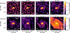 |
Fig. A.1. Continuum maps of the Circinus nucleus at the eight frequencies used for the SED decomposition presented in Sect. 4.1. All maps were convolved to a beam size of 74.5 × 65.2 mas2. We discern two emission components: free-free emission at the nucleus, which is visible in all bands, and dust emission, which is only visible in band 6, 7 and 9. We note that some extended emission is likely missing in the B6LB map because it has an MRS of 375 mas. This is likely also the reason for any discrepancy between this map and the one presented in Fig. 1. The synthesised beam sizes are drawn in the bottom left as filled ellipses, and the background rms values are shown in the bottom right in units of mJy/beam. |
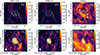 |
Fig. A.2. Band 7 HCO+(4-3) (νrest = 356.7 GHz), HCN(4-3) (νrest = 354.5 GHz), and CO(3-2) (νrest = 345.8 GHz) moment zero maps. We observe spiral structure in the CND that connects to the torus in all three transitions, with the bottom panels showing the inner bars of these hooks. Contour levels are drawn at [1, 2, 4, 8, 16, 32] × 50 mJy/beam km s−1 in the HCO+(4-3) and HCN(4-3) maps and at [1, 2, 4] × 300 mJy/beam km s−1 in the CO(3-2) maps. Cyan contours in the bottom left and middle panels indicate the position of the blueshifted emission feature discussed in Sect. 4.5 and represent the −30 km s−1 level in right panels of Fig. 8 for HCO+(3-2) and HCN(3-2), respectively. The synthesised beam sizes are drawn in the bottom left as filled ellipses, and the cyan cross indicates the AGN position. Indicated on the bottom panels are also the four locations where the 1D kinematic profiles from Fig. 10 were extracted using corresponding symbols in white. To boost the S/N in the moment zero maps, we applied a custom masking algorithm for the HCO+(4-3) and HCN(4-3) maps that conservatively masks out empty regions in the image cube. For CO(3-2), we masked out negative values in the image cube to remove artefacts caused by large scale emission that exceeds the maximal recoverable scale. Since this causes an upward bias in the flux density, the resulting CO(3-2) moment zero map is unsuitable for quantitative flux measurements. |
Appendix B: Continuum analysis
B.1. Possible synchrotron contribution in the mm regime from a jet or the X-ray corona
Based on the SED (Fig. 4), we find no clear evidence for synchrotron emission, which typically follows a power-law slope of α = −0.75 in the optically thin regime and α = 2.5 when optically thick (Rybicki & Lightman 1979). Synchrotron emission from a compact nuclear jet can, however, produce a flat spectrum at millimetre wavelengths, as is commonly observed in AGNs (e.g. Kaiser 2006; Kawamuro et al. 2022). Such emission is characterised by high brightness temperatures, typically TB > 107 K (Panessa et al. 2019). In our highest-resolution map (B6LB; 14.3 × 12.2 mas2), the peak flux density is 1.26 × 10⁻² Jy/beam, corresponding to an antenna temperature of TA = 1.3 × 10³ K. Since the brightness temperature of the resolved emission remains below this peak value, synchrotron radiation is unlikely to dominate there. The central core is unresolved, however, which leaves open the possibility that TB ≫ TA12. A relevant analogue where this central core component is resolved is NGC 1068, which is also known to contain a nuclear jet. In NGC 1068, Gallimore et al. (2004) identified a similar parsec-scale free-free emitting region (component “S1”) with TB = 4 × 10⁶ K that originates near the X-ray-irradiated maser disc. In that case, the free-free component dominates over the synchrotron jet in the mm continuum (Mutie et al. 2025). Since no jet has been observed in Circinus, we expect that any jet contribution in Circinus is even weaker than in NGC 1068. We therefore interpret the unresolved mm-core emission as arising from free-free processes in the X-ray corona or the maser disc, rather than from a nuclear jet (see also Blundell & Kuncic 2007).
In addition to a nuclear jet, X-ray coronae can also contribute to the synchrotron emission observed in AGNs (see e.g. Inoue et al. (2020) and Mutie et al. (2025) in the case of NGC 1068). In fact, based on the empirical correlation between X-ray and mm brightness from Ricci et al. (2023) and the observed X-ray flux of F2 − 10 keV = [1.3 − 2.6]×10−11 erg cm−2 s−1 for the Circinus AGN (Beckmann et al. 2006; Shu et al. 2011; Rivers et al. 2011; Yang et al. 2009), we expect a self-absorbed synchrotron component of F100 GHz = [1.9 − 33] mJy to exist in Circinus that peaks at mm wavelengths. Since we do not observe a peaked synchrotron component in the SED, we conclude that if present, it must be significantly weaker than the free-free component in the unresolved core. We therefore conclude that the nuclear continuum emission is largely dominated by optically thin thermal free-free emission between 86 GHz and 665 GHz and does not contain a significant contribution from synchrotron radiation.
B.2. Matching the VLBI maser astrometry to that of B6LB
The VLBI masers from McCallum et al. (2009) presented in Sect. 4.2.1 have small relative positional uncertainty (∼0.1 mas) but lack absolute astrometry. To solve this, we matched the position of the brightest 22 GHz maser from McCallum et al. (2009) to the astrometry of the brightest 183 GHz maser from S. Venselaar et al. (in prep.), which have almost the same radial velocity (vr,22 GHz = 126.5 km s−1 and vr,183 GHz = 125.4 km s−1) and overall position in the disc and can thus be assumed to belong to the same maser cloud. We then matched the astrometry from S. Venselaar et al. (in prep.) to that of B6LB by aligning the 183 GHz continuum peak to the position of the continuum peak in B6LB. We estimate that the resulting astrometric uncertainty of the maser positions on our B6LB map is ∼6 mas. From the relative maser positions, we can also derive an estimate for the position of the kinematic centre. To do this, we followed the method from Greenhill et al. (2003) by taking the average position of the innermost blueshifted and redshifted 22 GHz masers. We find that the kinematic centre is located 5.3 ± 6.0 mas to the north-west of the continuum peak, which is an insignificant offset within the relative astrometric uncertainty.
Appendix C: Additional kinematic modelling
C.1. Major axis PV diagram
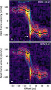 |
Fig. C.1. Position-velocity (PV) diagrams along the major axis for HCO+(3-2) (top, PA = 216°) and HCN(3-2) (bottom, PA = 217°) in the B6SB dataset. The colour map and black contours represent the data, and the cyan contours represent the model. Both sets of contours are drawn at [1, 2, 4, 8]×1.5 mJy/beam. Overlaid on the PV diagrams are also the fitted line-of-sight velocities VLOS = sin(i)×Vrot using cyan circles and the theoretical Keplerian profile of a central SMBH with a mass of M• = 1.7 × 10⁶ M⊙ (Greenhill et al. 2003) using a solid red curve. The size of the torus, which is barely resolved in B6SB, is indicated on the edges of each panel using vertical cyan markers. A white arrow is drawn in both panels to indicate the location of a < − 100 km s−1 blueshifted emission component in the data that is not replicated by the model. The synthesised beam sizes are shown in the bottom left as white bars. |
The major axis PV diagram presented in Fig. C.1 shows that the 3DBAROLO model is generally able to reproduce the kinematics observed in the CND along the major axis. However, within the central parsec, we see that the model is not able to properly reproduce the double-peaked kinematic profile and instead smears into one broad component. This inability is likely due to the inhomogeneous structure of the torus emission, which is unresolved in B6SB. Because 3DBAROLO has no knowledge of spatial emission structure that is smaller than the beam size, it assumes that the inner ring has a homogeneous flux density, which includes both the receding and approaching sides of the torus and portions of the disc that are at systemic velocity. However, we know from the moment zero maps of B6LB (bottom panels in Fig. 3) that this assumption is false and that the regions with a systemic line-of-sight velocity (along the minor axis) are weaker or completely missing due to the central absorption feature, especially in HCN(3-2). Looking at the PV diagrams in Fig. C.1, we see that indeed this gap in the data at systemic velocity is stronger in HCN(3-2) than in HCO+(3-2). We do not expect this discrepancy between the model and the data to have an effect on the modelling of the surrounding CND. Another discrepancy is the blue wing that we observe towards the torus (indicated with a white arrow in Fig. C.1). This blue wing causes an asymmetry in the torus spectrum between both sides of the torus. Its origin remains unclear, but possible reasons may be that we see fast-moving gas clouds that are orbiting the SMBH at the inner edge of the torus or, alternatively, a molecular outflow that is launched near the AGN.
C.2. Sensitivity of residual velocities to model parameters
To test whether the strong residuals described in Sect. 4.4 are the result of improper modelling of (a part of) the disc, we experimented with fixing different model parameters. Changing Vsys shifts the residuals, causing the blue (red) residuals to be stronger when choosing a higher (lower) Vsys. It is impossible to get rid of either the blue or red residuals completely without causing the rest of the disc to show a general residual blue or redshift that implies an improper value of Vsys. Forcing the PA to be 190° instead of 218 ± 6° eliminates the north-western blue and southern red residuals. However, this in turn creates a strong dipole in the residuals along the previously fitted position angle of 218 ± 6° at all radii, indicating that this fails to properly model the dominant rotation of the disc. Changing the inclination also changes the magnitude of the NW blue and S red residuals, with a larger (smaller) inclination angle producing larger (smaller) residuals. However, one needs to force the inclination angle to be i ≤ 50° for the blue and red residuals to become insignificant compared to the other residual velocities in the disc, at which point the expected disc morphology does not match the observed oblateness of the CND. In addition, the inclination would have to differ significantly from the values found by T22 and Curran et al. (1998) (i = 75 ± 5°) at the same spatial scale, Izumi et al. (2018) (i ≈ 70 ± 5°) at the 100 pc scale and by I23 (i ∼ 82°) at the parsec scale, which we consider unrealistic. Lastly, we experimented with only fitting the approaching or receding sides of the CND with 3DBAROLO. We find that the fit is robust against fitting only one side and that, consequently, the observed blue and red residuals do not change significantly. We therefore conclude that the observed velocity residuals are not the result of improper modelling.
C.3. Kinematic modelling with non-zero radial velocity
In order to check whether the 3DBAROLO tilted ring fit favours net inflow within the CND when we allow the model to include radial in- or outflow, we perform a second fit. We use the exact same setup as in Sect. 4.4, except that we leave Vrad as a free parameter with an initial guess of Vrad = 0. The resulting radial parameter profiles, the velocity fields and the 1D kinematic profiles extracted from the four point apertures are presented in Figs. C.2, C.3 and C.4, respectively.
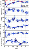 |
Fig. C.2. Same as Fig. 9, but for Vrad left as a free parameter. The fitted radial Vrad profile is shown in the fifth panel, where we define Vrad such that negative (positive) values imply inflow (outflow). In the bottom panel, we show the radial inflow rate that results from multiplying Vrad(r) by the radial mass distribution dMMN(r)/dr of the SMBH + Miyamoto-Nagai disc model (dashed red curve in the top panel, which was fitted to the rotation curve for Vrad = 0, see Sect. 4.5.1). |
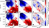 |
Fig. C.3. Same as Fig. 8, but for Vrad left as a free parameter. We find that the velocity residuals become smaller in general, with the blue residual being significantly less pronounced. |
We find that the fitted parameters are in general very similar to those for the initial fit without Vrad (i.e. Vrad = 0), except for the rotation velocities of the inner three rings, which are lower than for Vrad = 0. Since the projected minor axes of these rings are unresolved, we suspect that the model is not able to properly distinguish between Vrot, Vdisp, and Vrad at this inner region. We therefore do not trust these fitting results for the inner rings13. In the bottom panel of Fig. C.2, we show the radial inflow rate. This was calculated using
![Mathematical equation: $$ \begin{aligned} \begin{aligned} \dot{M}_{\mathrm{inflow} }(r) = -V_{\mathrm{rad} }(r)\times \frac{d}{dr}\left[M_{\mathrm{MN} }(r)\right], \end{aligned} \end{aligned} $$](/articles/aa/full_html/2025/12/aa55556-25/aa55556-25-eq7.gif) (C.1)
(C.1)
where MMN(r) is the mass enclosed within radius r in the Miyamoto-Nagai model based on the rotation curve from the 3DBAROLO fit with Vrad = 0.
The residual velocity fields and 1D kinematic profiles (Figs. C.3 and C.4) show that the model where Vrad was left free fits the observed kinematics better. We find that the residuals in the velocity field are significantly smaller (∼25 km s−1 rather than ∼40 km s−1 in the NW hook), and we find that the 1D kinematic profiles are better fitted when leaving Vrad free. However, the blue and red residuals along the NW hook and the E ridge do not disappear completely, and the northern point aperture still shows a significant discrepancy in Fig. C.4. From this, we conclude that the kinematics of the CND is more complex than a simple axisymmetric radial inflow and that the inflow through the spiral structure is faster than the average axisymmetric inflow modelled by 3DBAROLO, meaning that the majority of feeding happens through the spiral arms.
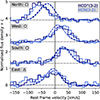 |
Fig. C.4. Same as Fig. 8, but for Vrad left as a free parameter. We find that the model better represents the 1D kinematic profiles at these four positions but that the model is still unable to produce a sufficiently blueshifted profile in the northern point aperture. |
C.4. Mass inflow as a function of radius
The resulting mass inflow profile (bottom panel Fig. C.2) is relatively flat between a radius of r = 3 pc and r = 14 pc at ![Mathematical equation: $ \dot{M}_{\mathrm{inflow}}=V_{\mathrm{rad}}(r)\times d/dr\left[M_{\mathrm{M-N}}(r)\right]\times f_{\mathrm{gas}} = 7.5\pm1.5\,\mathrm{M}_{\odot}\mathrm{yr}^{-1} $](/articles/aa/full_html/2025/12/aa55556-25/aa55556-25-eq8.gif) . The inner two rings show a significantly lower inflow rate. We again do not consider these values trustworthy since the sizes of their projected minor axes are unresolved. We also observe a drop in the inflow rate beyond r ≈ 14 pc. Taken at face value, this could be interpreted as a disruption of the supply of new material outside of this radius or that, assuming steady state, the molecular backflow of the fountain falls back around r ∼ 14 pc, causing the inflow to be larger inside than outside r ∼ 14 pc. We need to be cautious, however, since we also observe that the disc structure becomes more complex at this distance (see Figs. 3 and A.2). Outside of r ∼ 14 pc, larger-scale nuclear arms merge with the CND, which we expect to disrupt the dynamics of the disc. In addition, the ‘SW ridge’ is located around this distance, which contains two distinct velocity components (T22). The 3DBAROLO model is not designed to handle such kinematic complexity. Therefore, we do not consider the mass inflow rates at radii larger than ∼14 pc trustworthy.
. The inner two rings show a significantly lower inflow rate. We again do not consider these values trustworthy since the sizes of their projected minor axes are unresolved. We also observe a drop in the inflow rate beyond r ≈ 14 pc. Taken at face value, this could be interpreted as a disruption of the supply of new material outside of this radius or that, assuming steady state, the molecular backflow of the fountain falls back around r ∼ 14 pc, causing the inflow to be larger inside than outside r ∼ 14 pc. We need to be cautious, however, since we also observe that the disc structure becomes more complex at this distance (see Figs. 3 and A.2). Outside of r ∼ 14 pc, larger-scale nuclear arms merge with the CND, which we expect to disrupt the dynamics of the disc. In addition, the ‘SW ridge’ is located around this distance, which contains two distinct velocity components (T22). The 3DBAROLO model is not designed to handle such kinematic complexity. Therefore, we do not consider the mass inflow rates at radii larger than ∼14 pc trustworthy.
We expect the derived total inflow rates to be an overestimate because the kinematics based on HCO+(3-2) and HCN(3-2) traces high-density gas, which is predominantly concentrated in the spiral arms. When multiplying Vrad by the density of the Miyamoto-Nagai model, which contains all material (high- and low-density gas), we effectively assume that all material is falling in at the same velocity as the high-density gas. This is unlikely, since we observe Vrad to be higher in the denser spiral structures (e.g. Vrad = −43 km s−1 in the NW hook) compared to the disc average (Vrad ∼ −12 km s−1, Sect. C.3). This causes an upward bias in the total inflow rate calculated using Eq. C.1.
All Tables
All Figures
|
Fig. 1. Band 6 short (top) and long (bottom) baseline continuum maps at 259 GHz. Contour levels are drawn at [2, 4, 8, 16, 32, 64, 128, 256, 512, 1024] × rms, where the background rms equals 0.022 mJy/beam in the B6SB map and 0.013 mJy/beam in the B6LB map. The synthesised beam sizes are drawn in the bottom left as filled ellipses, and the cyan cross indicates the AGN position (as defined in Sect. 3.4). The phoenix feature is indicated with a white arrow. The polar and equatorial directions mentioned throughout the text are shown in the upper panel. |
| In the text | |
|
Fig. 2. Spiral structures in the CND (as informed by the morphology in Figs. 3 and A.2) overlaid on the band 7 CO(3-2) (νrest = 345.8 GHz) map. The dashed cyan arrow represents the proposed inflow through the NW hook that feeds the torus as discussed in Sect. 4.5. The synthesised beam size is drawn in the bottom left as a filled ellipse, and the cyan cross indicates the AGN position. |
| In the text | |
|
Fig. 3. Band 6 HCO+(3-2) (νrest = 267.6 GHz) and HCN(3-2) (νrest = 265.9 GHz) short (top, covering the CND) and long (bottom, showing the resolved torus) baseline moment zero maps. Contour levels are drawn at [ − 16, −8, −4, 2, 4, 8, 16] × rms, where the background rms equals 36, 23, 57 and 28 mJy/beam km/s in the HCO+(3-2) B6SB and B6LB and HCN(3-2) B6SB and B6LB maps, respectively. White contours represent negative flux density values and indicate the position of an absorption hole that coincides with the continuum peak. The L-shape that contains the NW and SW hooks as discussed in the text is drawn as dashed black lines in the top panels. Cyan contours in the top panels indicate the position of the blueshifted emission feature discussed in Sect. 4.5 and represent the −30 km s−1 level in the right panels of Fig. 8. The synthesised beam sizes are drawn in the bottom left as filled ellipses, and the cyan cross indicates the AGN position. |
| In the text | |
|
Fig. 4. Spectral energy distribution of the Circinus AGN for the three apertures drawn in Fig. 5. Also shown are four ATCA measurements at varying beam sizes (Elmouttie et al. 1998) in white. The dashed lines represent a power-law (Fν ∝ να) fit of the 300 mas nuclear aperture containing both a dust component with α = 3.5 and a free-free component with α = −0.1. We also plot the nuclear dust model by Stalevski et al. (2019) in orange. |
| In the text | |
|
Fig. 5. Band 6 (259 GHz) continuum decomposed into a free-free (α = −0.1) and a dust (α = 3.5) component based on pixel-by-pixel SED-fitting. The common beam size between all maps used for these SED fits is drawn in the bottom left as a filled ellipse. In the left figure, we indicate the Phoenix and the two nuclear apertures used to obtain the spectral energy distribution shown in Fig. 4. |
| In the text | |
|
Fig. 6. Ionised gas morphology (traced by the 259 GHz continuum) compared to the dusty outflow cone (traced by the mid-IR N-band continuum from Isbell et al. 2022, top panel) and the accretion disc and molecular outflow (traced by the 22 GHz mega-masers from McCallum et al. 2009, middle panel). The B6LB 259 GHz continuum (robust parameter = 0.5) is drawn in the top panel as cyan contours at [4, 8, 16, 32, 64, 128, 256, 512] × rms, with rms = 0.013 mJy/beam. The B6LB and N-band continuum synthesised beam sizes are shown on the bottom left and right, respectively. The middle panel shows the higher resolution (robust parameter = −1) B6LB continuum map with contour levels at [2, 4, 8, 16, 32, 64, 128] × rms, with rms = 0.048 mJy/beam. Overlaid on the middle panel are the 22 GHz maser spots that trace the Keplerian disc (black edge) and the outflow (white edge). The maser spots have a global positional uncertainty of ∼6 mas. The solid cyan lines indicate the fitted outflow trajectories, whereas the dashed cyan lines show these trajectories extrapolated to the maser disc. The orange cross indicates the maser kinematic centre, while the cyan cross indicates the AGN position. The bottom panel shows a schematic representation of the proposed outflow cone geometry. The sketched torus component is based on the B6LB torus morphology in Fig. 3. The grey labels ‘N’ (near) and ‘F’ (far) indicate the respective sides of the warped accretion disc: N marks the near side that is in the line of sight of the AGN, while F corresponds to the far side that is in shadow, as discussed in Sect. 4.2.3. |
| In the text | |
|
Fig. 7. Top panel: Phoenix feature as observed in the B6SB 259 GHz continuum compared to the B7 CO(3-2) molecular tracer (blue contour at 1.0 mJy/beam km/s). We observe a mismatch between the continuum and CO(3-2) morphology, which either implies that the Phoenix feature is associated with a polar outflow perpendicular to the CND or that the inner spiral arm structure traced by dust differs from the molecular spirals. Bottom panel: Illustration of both of these scenarios. The spiral pattern drawn in purple is based on the structure observed in the right panel of Fig. 5. The B6SB 259 GHz continuum contours are drawn at [6, 8] × rms, with rms = 0.022 mJy/beam. |
| In the text | |
|
Fig. 8. Velocity fields of the CND for HCO+(3-2) (top) and HCN(3-2) (bottom) from the B6SB dataset as observed (left), as modelled using 3DBAROLO (middle) and the residual velocity field that results from subtracting the model from the data (right). The black arrows in the right panels indicate the position of the blue residual feature that coincides with the position of the NW hook. Velocity contour levels are drawn at [ − 75, −50, −25, 0, 25, 50, 75] km s−1. The rest frame velocity is defined relative to Vsys = 441.4 km s−1. Indicated on all maps are the point apertures used to extract the 1D kinematic profiles shown in Fig. 10 using corresponding symbols in white. The synthesised beam sizes are drawn in the bottom left as filled ellipses, and the cyan cross indicates the AGN position. |
| In the text | |
|
Fig. 9. Fitted kinematic and morphological radial parameters of the CND from 3DBAROLO modelling of the HCO+(3-2) and HCN(3-2) transitions in the B6SB dataset. The top two panels show the 3DBAROLO fitting results and the associated uncertainties after the second fitting iteration, while the bottom two panels show the fit results and uncertainties from the first iteration as scatter points with the regularised radial parameter profiles overlaid as solid curves that are used in the second iteration. The SMBH + Miyamoto-Nagai disc rotation curve fit is overlaid in the top panel as a red dashed line. |
| In the text | |
|
Fig. 10. Kinematic 1D profiles of HCO+(3-2) and HCN(3-2) in B6SB extracted from the four point apertures as indicated in Fig. 8 using corresponding markers. We show the data as a step curve and the 3DBAROLO model as dashed curves. The 1D kinematic profiles are normalised by the maximal flux density in the model. The spectra are offset by a term c as indicated by the horizontal dotted lines. |
| In the text | |
|
Fig. A.1. Continuum maps of the Circinus nucleus at the eight frequencies used for the SED decomposition presented in Sect. 4.1. All maps were convolved to a beam size of 74.5 × 65.2 mas2. We discern two emission components: free-free emission at the nucleus, which is visible in all bands, and dust emission, which is only visible in band 6, 7 and 9. We note that some extended emission is likely missing in the B6LB map because it has an MRS of 375 mas. This is likely also the reason for any discrepancy between this map and the one presented in Fig. 1. The synthesised beam sizes are drawn in the bottom left as filled ellipses, and the background rms values are shown in the bottom right in units of mJy/beam. |
| In the text | |
|
Fig. A.2. Band 7 HCO+(4-3) (νrest = 356.7 GHz), HCN(4-3) (νrest = 354.5 GHz), and CO(3-2) (νrest = 345.8 GHz) moment zero maps. We observe spiral structure in the CND that connects to the torus in all three transitions, with the bottom panels showing the inner bars of these hooks. Contour levels are drawn at [1, 2, 4, 8, 16, 32] × 50 mJy/beam km s−1 in the HCO+(4-3) and HCN(4-3) maps and at [1, 2, 4] × 300 mJy/beam km s−1 in the CO(3-2) maps. Cyan contours in the bottom left and middle panels indicate the position of the blueshifted emission feature discussed in Sect. 4.5 and represent the −30 km s−1 level in right panels of Fig. 8 for HCO+(3-2) and HCN(3-2), respectively. The synthesised beam sizes are drawn in the bottom left as filled ellipses, and the cyan cross indicates the AGN position. Indicated on the bottom panels are also the four locations where the 1D kinematic profiles from Fig. 10 were extracted using corresponding symbols in white. To boost the S/N in the moment zero maps, we applied a custom masking algorithm for the HCO+(4-3) and HCN(4-3) maps that conservatively masks out empty regions in the image cube. For CO(3-2), we masked out negative values in the image cube to remove artefacts caused by large scale emission that exceeds the maximal recoverable scale. Since this causes an upward bias in the flux density, the resulting CO(3-2) moment zero map is unsuitable for quantitative flux measurements. |
| In the text | |
|
Fig. C.1. Position-velocity (PV) diagrams along the major axis for HCO+(3-2) (top, PA = 216°) and HCN(3-2) (bottom, PA = 217°) in the B6SB dataset. The colour map and black contours represent the data, and the cyan contours represent the model. Both sets of contours are drawn at [1, 2, 4, 8]×1.5 mJy/beam. Overlaid on the PV diagrams are also the fitted line-of-sight velocities VLOS = sin(i)×Vrot using cyan circles and the theoretical Keplerian profile of a central SMBH with a mass of M• = 1.7 × 10⁶ M⊙ (Greenhill et al. 2003) using a solid red curve. The size of the torus, which is barely resolved in B6SB, is indicated on the edges of each panel using vertical cyan markers. A white arrow is drawn in both panels to indicate the location of a < − 100 km s−1 blueshifted emission component in the data that is not replicated by the model. The synthesised beam sizes are shown in the bottom left as white bars. |
| In the text | |
|
Fig. C.2. Same as Fig. 9, but for Vrad left as a free parameter. The fitted radial Vrad profile is shown in the fifth panel, where we define Vrad such that negative (positive) values imply inflow (outflow). In the bottom panel, we show the radial inflow rate that results from multiplying Vrad(r) by the radial mass distribution dMMN(r)/dr of the SMBH + Miyamoto-Nagai disc model (dashed red curve in the top panel, which was fitted to the rotation curve for Vrad = 0, see Sect. 4.5.1). |
| In the text | |
|
Fig. C.3. Same as Fig. 8, but for Vrad left as a free parameter. We find that the velocity residuals become smaller in general, with the blue residual being significantly less pronounced. |
| In the text | |
|
Fig. C.4. Same as Fig. 8, but for Vrad left as a free parameter. We find that the model better represents the 1D kinematic profiles at these four positions but that the model is still unable to produce a sufficiently blueshifted profile in the northern point aperture. |
| In the text | |
Current usage metrics show cumulative count of Article Views (full-text article views including HTML views, PDF and ePub downloads, according to the available data) and Abstracts Views on Vision4Press platform.
Data correspond to usage on the plateform after 2015. The current usage metrics is available 48-96 hours after online publication and is updated daily on week days.
Initial download of the metrics may take a while.