| Issue |
A&A
Volume 704, December 2025
|
|
|---|---|---|
| Article Number | A204 | |
| Number of page(s) | 16 | |
| Section | Stellar structure and evolution | |
| DOI | https://doi.org/10.1051/0004-6361/202556154 | |
| Published online | 10 December 2025 | |
VLTI observations of Orion Belt stars
I. ε Orionis★
1
Charles University, Faculty of Mathematics and Physics, Astronomical Institute, V Holešovičkách 2, CZ-180 00 Praha 8-Trója, Czech Republic
2
European Southern Observatory, Karl-Schwarzschild-Str. 2, D-85748 Garching, Germany
3
Department of Physics and Astronomy, University of North Carolina at Chapel Hill, Chapel Hill, NC 27599, USA
★★ Corresponding author: This email address is being protected from spambots. You need JavaScript enabled to view it.
Received:
27
June
2025
Accepted:
15
October
2025
Abstract
Massive stars play a decisive role in the evolution of the Universe. They are the primary sources of ionising radiation, generating strong stellar winds that affect the interstellar medium. They ultimately end their lives as supernovae, ejecting synthesised, r-process elements.
Key words: techniques: interferometric / stars: massive / stars: individual: Orion Belt / stars: individual: Eps Ori
Based on ESO proposal 112.25JX, PI A. Oplištilová.
© The Authors 2025
 Open Access article, published by EDP Sciences, under the terms of the Creative Commons Attribution License (https://creativecommons.org/licenses/by/4.0), which permits unrestricted use, distribution, and reproduction in any medium, provided the original work is properly cited.
This article is published in open access under the Subscribe to Open model. This email address is being protected from spambots. You need JavaScript enabled to view it. to support open access publication.
1. OB stars in Orion’s Belt
O- and B-type (OB) stars have relatively short lifetimes, lasting only a few million or tens of millions of years, yet they are crucial cosmic engines with a long-lasting influence on the evolution of the Universe. They exert strong feedback on their environment, not only as sources of energy, ionising photons, chemical elements through winds or core-collapse supernova (SN) explosions (Clayton 1983), but also as precursors of neutron stars, black holes, and, consequently, gravitational wave sources (Marchant et al. 2021).
The most likely precursors include overcontact binaries (Almeida et al. 2015), X-ray binaries (Atri et al. 2019), quiescent binaries (Shenar et al. 2022), or pair-instability SNe (Renzo et al. 2022). Various formation channels must be constrained by photonic observations. The distribution of black hole masses (Abbott et al. 2021) indicates a hierarchical merging. This is complicated by ‘kicks’ of the order of 100 km/s, during explosions (Wongwathanarat et al. 2013) or mergers (Shenar et al. 2022). The kicks can be compensated by the escape velocity from nuclear clusters or the escape velocity from multiple systems, where the radial velocities (RVs) of components are comparable to the kick velocities.
One particularly characteristic aspect of massive stars is their multiplicity: 90% of massive, hot OB stars possess at least one stellar companion (Sana et al. 2014; Sota et al. 2014; Maíz Apellániz et al. 2019; Pauwels et al. 2023), which influences their evolution throughout their lives. Yet, some stars remain single (e.g. ε Ori), even though they share the same birth environment with multiple systems. Considering the possible interactions among stars, they might be the result of a more complicated evolutionary process, including mass transfer or mergers resulting from close encounters between stars.
The evolution of massive stars still remains poorly constrained by observations. The primary kind of observation constraining diameters is long-baseline interferometry. While the most massive stars in the Large Magellanic Cloud, such as BAT99-98 with M ≈ 200 M⊙ located in the Tarantula nebula (30 Dor, Hainich et al. 2014; Kalari et al. 2022), are too distant (50 kpc) for interferometric measurements, the Orion OB1 association at about 400 pc from us seems to be a perfect region for the investigation of questions related to the birth of OB stars and their evolution.
The brightest stars in Orion’s Belt, members of the OB1b Orion association, δ Ori, ζ Ori, σ Ori, and ε Ori with individual component masses of up to 35 M⊙ (Hummel et al. 2013; Schaefer et al. 2016; Puebla et al. 2016; Oplištilová et al. 2023) represent massive stars that are accessible to the most advanced optical interferometers. The parallaxes of faint stars surrounding the aforementioned bright stars were measured in Gaia DR3 (Gaia Collaboration 2021); the corresponding distances are all around 0.38 kpc (Oplištilová et al. 2023). It is thus possible to measure their angular separations and angular diameters.
In this first paper, we focus on ε Ori (Alnilam, 46 Ori, HD 37128), which is the largest and brightest star in Orion’s Belt. Based on photometric measurements taken at the Hvar Observatory (Božić & Harmanec 2023), its standard magnitudes are: V = 1.691 mag, B = 1.509 mag, and U = 0.495 mag. In the near-infrared (NIR, the passband of PIONIER), the magnitude is H = 2.07 mag (Ducati 2002a). It is classified as a B0 Ia blue supergiant and represents the only massive single star in Orion’s Belt. Its mass of about 30 M⊙ (Puebla et al. 2016) is similar to the total masses of the other multiple systems in Orion. Also, it has an intense wind (Puebla et al. 2016) and a mass-loss rate of up to ̇M = 5.25 ⋅ 10−6 M⊙ yr−1 (Repolust et al. 2005). It might be the case that ε Ori is a post-mass-transfer object, and represents a future evolved state of multiple stellar systems in Orion. For this reason, we include a brief discussion of the relevant systems, δ, ζ, and σ Ori, to enable a comparison of their masses, radii, spectral types, and so on.
δ Ori (Mintaka, HD 36486, HR 1852/1851) is our closest massive multiple system consisting of five components in total: [(Aa1 + Aa2) + Ab] + (Ca +Cb). The triple star A (O9.5 II + B2 V +B0 IV) has the periods P1 = 5.732436 d, P2 = 55 450 d and the mass 17.8 + 8.5 + 8.7 ≃ 35 M⊙ (Oplištilová et al. 2023). The primary (Aa1) is an unusually evolved O-type star. The star has been studied in a series of papers by Corcoran et al. (2015), Pablo et al. (2015), Nichols et al. (2015), and Shenar et al. (2015). We have already constructed a model of δ Ori A (Oplištilová et al. 2023), based on diverse observational data (photometry, astrometry, radial velocities, eclipse timings, eclipse duration, spectral line profiles, and spectral-energy distribution), with the exception of interferometry, as previous VLTI/AMBER data were not usable. One conclusion from that study was that the compact binary Aa1+Aa2 is a pre-mass-transfer object, while the tertiary seems to be unusually inflated (according to its log g and the HR diagram).
ζ Ori (Alnitak, 50 Ori, HR 1948/1949) consists of four components [((Aa + Ab) + B] + C, also includes a triple star O9.7 Ib + B0.5 IV + B0 III and, in particular, a double-lined spectroscopic binary with the mass 33 + 14 ≃ 47 M⊙ (Hummel et al. 2000). The 2 mag fainter companion Ab with the period P1 ≈ 2687 d, mean separation of 45 mas, and eccentricity e1 = 0.338 was discovered by Hummel et al. (2000). The primary Aa is the only known magnetic O-type supergiant. Tertiary B has a fast rotation of 350 km/s, separation of 2.4 arcsec, period P2 = 1509 yr, and eccentricity e2 = 0.07.
Finally, σ Ori (48 Ori, HD 37468, HR 1931) has six components [(Aa+Ab)+B] + C + D + E of spectral types [(O9.5 V+B0.5 V)+A2V] + B2V + B2V + ?. The triple star has masses of 17 + 13 + 12 ≃ 42 M⊙. Binary A (P1 ≈ 143 d) and component B form a visual pair with P2 ≈ 160 yr. The angular separations of all components are 4.3 mas, 260 mas, 11 arcsec, 13 arcsec, and 42 arcsec, respectively. Unlike δ Ori, the inner orbit of σ Ori is eccentric, while the outer is circular (Schaefer et al. 2016). According to Schaefer et al. (2016), the expected angular diameters are 0.27 and 0.21 mas for Aa and Ab, respectively. The system has already been observed by interferometers such as CHARA/MIRC, NPOI, and VLTI/AMBER; however, the diameters were unresolved.
In 2023, we succeeded with the ESO proposal (Programme ID: 112.25JX) to observe ε, δ, ζ, and σ Ori with the Very Large Telescope Interferometer (VLTI). The main goal was to resolve the angular diameters of individual components to constrain complex models of the stellar systems.
2. Observational data
Hereinafter, we describe the observational datasets, including interferometry from VLTI instruments, spectroscopy from CFHT and CTIO. We also describe the other datasets we used for the modelling ε Ori.
2.1. VLTI/GRAVITY interferometry
In our two runs of Programme ID: 112.25JX, (PI A. Oplištilová, 12 h + 1 h) – in phase 112, running between 1/10/23 and 31/3/24 at Cerro Paranal in northern Chile, we obtained observations of ζ, σ, and δ Ori with the GRAVITY instrument (Eisenhauer et al. 2011; GRAVITY Collaboration 2017) and observations of ε Ori with the PIONIER instrument (Le Bouquin et al. 2011). Both runs were performed in service mode. Such data should enable us to fit stars’ angular diameters and angular positions with up to an accuracy of 10 microarcseconds.
For observations with GRAVITY, we requested 12 concatenations, each including two observing blocks, science target and calibrator (CAL-SCI). Each concatenation lasted 1 h; thus, we obtained observations on four different nights for each target, 12 hours of observations in total. All our three targets were very bright; therefore, we used the auxiliary telescopes (ATs) with the extended configuration, which made these observations possible for the first time. We also permitted observations under the poorest conditions that still allow data acquisition; namely, a seeing of < 1.4 arcsec, variable sky with thin cirrus, and an air mass of 1.6. We chose the spectrometer with a high spectral resolution. The observations (time series) were carried out in single on-axis mode, with automatic fringe tracking, adaptive optics with Coude guiding, and standard calibration. For δ and σ Ori, we set the Wollaston spectrometer out and for ζ Ori, in. Otherwise, the brightest object ζ Ori would be saturating the instrument camera.
We performed the calibration using the EsoReflex GRAVITY pipeline (Freudling et al. 2013). The essence of calibration is to compare the observed visibilities of (partially resolved) calibrators (see Table 1 and Fig. 2), with the theoretical visibilities of the corresponding uniform disk, which is described by
 (1)
(1)
Epochs of interferometric observations and uniform-disk diameters (UDD) of calibrators.
where J1 is the Bessel function of the first order, the square root  corresponds to the length of a baseline, and θ is the angular diameter of the calibrator. The visibility function for a uniform disk is the simplest model, but it is sufficient for the calibration process. The larger the diameter, the faster the visibility drops as a function of the spatial frequency. The comparison of theoretical and observed visibilities is expressed by a transfer function as the ratio of the calibrator’s squared visibilities and theoretical squared visibilities,
 (2)
(2)
The transfer function is used to reduce raw uncalibrated data; the reduced data, V*2, are the ratio of raw data and the transfer function,
 (3)
(3)
For all three objects, we obtained squared visibilities measured on six baselines, covering the wavelength range from 1.95 μm to 2.45 μm. The coverage of measurements in uv-planes for each target is shown in Fig. 1, and examples of reduced squared visibilities, V2, and the corresponding calibrators’ visibilities are in Fig. 2. We also obtained closure phases for four triangles composed of these six baselines. We checked the closure phases of calibrators, which were close to zero as expected, indicating the central symmetry, characteristic of single, unspotted stars.
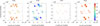 |
Fig. 1. Coverage for interferometric measurements showing the squared visibility V2 vs baselines (u,v) ≡ B/λ in cycles per baseline. Individual panels show four stars in Orion’s Belt (ζ, σ, ε, and δ Ori). For each star, all nights are plotted. Colours correspond to visibility values. |
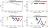 |
Fig. 2. Examples of reduced squared visibilities, V2, of the science targets, ε, δ, ζ, and σ Ori. Measurements are from nights: 20 November 2023, 22 November 2023, 8 January 2024, and 23 November 2023, respectively. Science targets are with obvious signals from companions. For the single star ε Ori, the signal suggests an elongated or non-spherical shape, unlike the calibrator ζ Lep, which exhibits a perfectly spherical shape. Colours correspond to individual baselines. The squared visibilities of calibrators are in Fig. C.3. |
In the case of ζ Ori and its calibrator, we obtained two polarisation directions, P1 and P2, thanks to the Wollaston prism. However, since the object does not have a strong magnetic field, we cannot use the polarimetric data to determine any properties. The Wollaston prism was used just to prevent saturation of this bright target. For more information on the calibration of ζ Ori, we refer to Appendix A.
2.2. VLTI/PIONIER interferometry
With the PIONIER instrument, we proposed a single concatenation composed of three observing blocks (CAL-SCI-CAL) in an extended configuration with ATs. We obtained six interferometric measurements of ε Ori on six baselines, within one hour of observing time. This resulted in a total of 36 squared visibility and 24 closure phase measurements. To obtain this snapshot, we applied for the grism as the disperser for PIONIER. The PIONIER instrument works in the H-band (1.52–1.76) μm, which delivers a better angular resolution than GRAVITY for measuring a single star diameter. The target is very bright; thus, observations could be conducted under relaxed weather constraints: seeing < 1.15 arcsec, variable sky with thin cirrus, and an air mass of 2.0. Again, the observations were obtained with automatic fringe tracking, adaptive optics with Coude guiding, and standard calibration. Data reduction was performed using the Pndrs software (Le Bouquin et al. 2011). The uv-plane coverage is shown in Fig. 1, and the reduced squared visibilities, V2, together with those of the calibrator ζ Lep (Table 1) are shown in Fig. 2.
2.3. CTIO/CHIRON and CFHT Spectroscopy
We obtained four echelle spectra of the spectral range (4504–8900) Å at the Cerro Tololo Inter-American Observatory (CTIO) with the 1.5-m reflector using the highly stable cross-dispersed echelle spectrometer CHIRON. We used the fibre mode with the resolution of R ≈ 25 000. A preliminary reduction to 1D spectra was carried out at CTIO (Tokovinin et al. 2013). We performed rectification using the reSPEFO2 software written by A. Harmanec1.
Additionally, we used four spectra measured by the 3.6-m Canada-France-Hawaii Telescope (CFHT), located near the summit of Mauna Kea on Hawaii. The spectra from the ESPaDOnS instrument cover the region of (3815–6600) Å and have the resolution of 68 000. These archival spectra have relatively low uncertainties in the normalised intensity, less than 0.01, corresponding to photon noise for bright stars. Due to remaining rectification systematics, we added a value of 0.01 to uncertainties.
2.4. Spectral energy distribution (SED)
To compute the SED, we downloaded absolute fluxes from the photometric catalogues in the VizieR tool (Allen et al. 2014). We selected all measurements within the wavelength range of the BSTAR absolute synthetic spectra. Specifically, we obtained measurements between 0.353 and 2.1 μm in the standard Johnson photometric system (Ducati 2002b), along with measurements from Gaia DR3 (Gaia Collaboration 2020) and 2MASS (Cutri et al. 2003). We omitted clear outliers and multiple entries. For measurements without reported uncertainties, we assumed the value of 0.02 mag. Hipparcos measurements were not used due to underestimated systematic uncertainties. The final dataset contained 13 data points see Table A.1.
To compute the reddening, EB − V, for ε Ori, we used the differential photometry measured in October 2006 and February 2024 (2454015.6–2460362.4 HJD) at the Hvar Observatory (Božić & Harmanec 2023); namely, the observed colour index (B − V)0 = −0.192 mag. For the corresponding spectral type B0Ia, the intrinsic colour is (B − V) = − 0.240, according to (Golay 1974) and, consequently, EB − V = 0.05 mag and AV = 0.155 mag, which is in agreement with Fan et al. (2017) and negligible in the infrared (IR).
For the construction of the SED, we also used calibrated UBV photometry from the Hvar differential archive. It contains 21 observations secured in 2006 by Petr Harmanec, Domagoj Ruždjak and Davor Sudar, and 4 observations secured during one night in 2024 by Hrvoje Božić. We used the mean values of all 25 observations, U = 0.479 ± 0.025, B = 1.487 ± 0.034, and V = 1.679 ± 0.018. The SED data were calculated using the wavelengths from Bessell (1939) and calibration fluxes from Wilson et al. (2010). The resulting values of SED are in Table A.1.
2.5. Parallax
As ε Ori is too bright, it saturates Gaia’s detector, designed primarily for stars fainter than G = 6 mag, and its parallax measurements are not reliable. Hipparcos parallaxes were less precise; Perryman et al. (1997) estimated the distance of 412 pc, while van Leeuwen (2007) 606 pc. Instead, in Oplištilová et al. (2023), we used Gaia DR3 parallaxes of the faint stars in the same stellar association (Orion OB1b), as these provide more precise and unbiased distance estimates than those available for the brightest members, which suffer from larger Gaia systematics. This approach yields a more reliable association distance. We assumed that the most massive stars are located close to the median distance (Kuhn et al. 2010, Sect. 9.3). Then the distance of ε Ori should be close to d ≃ 384 pc, which is just intermediate between the other Orion Belt stars, ζ Ori (386 pc) and δ Ori (381 pc).
As a verification, we checked diffuse interstellar bands (DIBs). Their strength depends on the interstellar medium (and not on the spectral type) and is correlated with the colour excess, EB − V, which quantifies the amount of dust and reddening along the line of sight (Friedman et al. 2011). We assumed that the interstellar medium in the direction of ε Ori has similar properties to other stars close on the sky. We used the same methodology as Guinan et al. (2012); we selected two stars (Table 2) that are not in a dusty region according to the WISE map (Baumann et al. 2022) and have both Gaia parallaxes and high-resolution spectra in public archives. Then, we compared the strengths of their DIBs (Fig. 3). The star HD 37140 shows significant DIBs at the distance of (420 ± 9) pc, while HD 36628 shows no DIBs at (242 ± 2) pc. ε Ori presents very low DIBs comparable to HD 37140; thus, we verified that ε Ori is likely located at the distance < 420 pc (see Table 2) and our previous estimate seems to be reasonable.
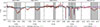 |
Fig. 3. Comparison of DIBs’ intensities for ε Ori and stars which are close on the sky (HD 37140 and HD 36628). The most distant star has the deepest DIBs, while the star with the lowest distance has very weak DIBs. The spectrum of ε Ori also shows weak DIBs, which suggests its distance is lower than 420 pc. The spectra were taken from public archives of CFHT and ESO. |
Distances and reddening of stars that are close to ε Ori on the sky.
Similarly, the colour excess EB − V is closely correlated with the distance. We thus computed EB − V, according to Johnson & Morgan (1953), using U, B, and V magnitudes from Blanco et al. (1970) and Mermilliod (1994), see Table 2. The colour excess of ε Ori is computed in Sect. 2.4. Moreover, according to Green et al. (2019)2, there is a sudden ‘jump’ in reddening in this direction, occurring at a distance of 400 pc.
We conclude that the previous distance estimate of about 600 pc is certainly incorrect. The relation of EB − V, the strengths of DIBs, and distance of ε Ori corresponds to our estimate, (384 ± 8) pc.
3. ε Ori as a single star
We constructed a single-star model of the B0 Ia supergiant ε Ori using PHOEBE23 (Prša et al. 2016; Horvat et al. 2018; Jones et al. 2020; Conroy et al. 2020). PHOEBE2 employs seamless triangular meshes, closely following the generalised Roche potential. Each triangular element of the mesh is assigned local quantities (e.g. temperature, surface gravity, intensity, directional cosine). The total flux is then computed by integrating over visible elements. PHOEBE2 incorporates various stellar atmosphere models, which enables a realistic, self-consistent treatment of limb darkening, gravity darkening, and rotational distortion. It is a powerful tool for solving an inverse problem, constrained by light curves and radial velocity curves, and, recently, it was extended to include interferometry, spectra, and SED.
Grid of almost spherical models for ε Ori assuming a fixed value of v sin i = 70 km s−1.
A new interferometric module in PHOEBE24 (Brož et al. 2025b) enables the computations of interferometric observables, squared visibility (V2), closure phase (argT3), and amplitude (|T3|), by means of the Fourier transform approach. Additionally, a new spectroscopic module (Brož et al. 2025a) utilises interpolations in grids of synthetic spectra, assigning one spectrum to each element. Again, the total spectrum is obtained by integrating over all elements, weighted by appropriate passband intensities. It enables the fitting of detailed spectral line profiles.
3.1. Visibility.
First, we modelled ε Ori as a spherical star with fixed radiative parameters according to Puebla et al. (2016); namely, T = (27 000 ± 500) K and log g = (3.00 ± 0.05) that they estimated by the fitting of line profiles of Hβ, Hγ, Hδ, and Hε. In PHOEBE2, we set the Kurucz atmospheres, but linear limb darkening coefficient c1 = 0.01621 interpolated from van Hamme (1993) tables for comparison purposes (see below). We assumed the distance d ≃ 384 pc, as discussed in Sect. 2.5. We verified the computation of V2 using the independent implementation of Brož (2017). The fit to V2 from PIONIER and the convergence of one free parameter (m) using the simplex method (Nelder & Mead 1965) resulted in exactly the same χVIS2 = 12.1 in both codes (Fig. C.2). The χ2 value is smaller than the number of degrees of freedom ν = N − M = 35, which most likely indicates overestimated uncertainties of PIONIER observations. In fact, previous PIONIER observations were more precise (Pietrzyński et al. 2019). We rescaled the uncertainties down by the factor of 12.1/35 (χ2/(N − M)). For the nominal uncertainties, we used the ones computed by the Pndrs pipeline, which calculates uncertainties of V2 from the frame-to-frame scatter of the raw coherence factor, and then propagates transfer function uncertainties (including calibrator diameter errors) into the final calibrated errors reported in OIFITS outcome of Pndrs pipeline. With these rescaled uncertainties, the best-fit mass is m = (23.5 ± 0.5) M⊙, corresponding to the angular diameter, θ = (0.615 ± 0.007) mas, and physical radius, R = (25.4 ± 0.3) R⊙.
Second, we modelled a rotating, almost spherical star. For simplicity, we used black-body atmospheres to avoid problems with too low log g values, occurring when the star is close to the critical rotation (cf. Fig. 4). Nevertheless, we derived the limb darkening coefficients from the Kurucz atmospheres and set them manually, with a power-law prescription (Prša et al. 2016) of
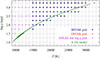 |
Fig. 4. Grids of synthetic spectra BSTAR and OSTAR (Lanz & Hubený 2003, 2007) used in our spectroscopic models. Each spectrum is parametrised by log g and T. To describe also critically rotating stars (cf. green points), it was necessary to compute additional ATLAS spectra (Castelli & Kurucz 2003) for low values of log g and T. |
 (4)
(4)
where c1 = 1.698, c2 = −4.151, c3 = 5.887, c4 = −2.525 are suitable for the temperature, T = 27 000 K and log g = 3.0 (Puebla et al. 2016). We set the bolometric gravity brightening exponent β = 1.0, which corresponds to hot stars (T > 8000 K). The exponent occurs in the implementation of local temperature in PHOEBE2 (von Zeipel 1924; Prša 2011; Prša et al. 2016), expressed as
 (5)
(5)
where g is the local gravitational acceleration. To reveal all possible minima of χ2, we computed a more detailed grid in the inclination of the rotation axis (hereafter only ‘inclination’) i. The orientation of the star is also determined by Ω, longitude of the ascending node (of the equator). We made the parameters m and Ω free, the parameters log g, d, v sin i (and i) fixed, while the dependent parameters Prot, Requiv, and θequiv were constrained by the following relations,
 (6)
(6)
 (7)
(7)
 (8)
(8)
where the value of v sin i was set up to 70 km s−1 (Puebla et al. 2016).
Grid of non-spherical models of ε Ori without a v sin i constraint.
The converged models for fixed values of i are listed in Table 3. Unfortunately, the models were too constrained by the fixed value of vsin i; the χVIS2 dependence on i remained flat over the full range of i. Formally, the lowest χVIS2 value is for the lowest inclination, i = 14 deg. Lower values of i cause problems in the modelling of edges. For the best-fit model, converged from parameters with the lowest χVIS2, we refer to Fig. 5. It is an almost spherical star close to critical rotation, with almost pole-on orientation.
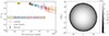 |
Fig. 5. Almost spherical model of ε Ori based on PIONIER observations in H-band with fixed v sin i (Puebla et al. 2016). Left: Squared visibility vs projected baseline B/λ. Right: Corresponding triangular mesh with the passband intensities (greyscale). The model was converged starting with the parameters from Table 3 (bold line). The best-fit was with χVIS2 = 11.23. The free parameters were i = 13.6 deg, m = 20.3 M⊙, Ω = 293.7 deg, Prot = 4.01 d. The fixed parameters were v sin i = 70 km s−1, T = 25 000 K, γ = 25.9 km s−1 and the derived parameters were v = 298 km s−1, Requiv = 22.43 R⊙(derived), Rpole = 22.29 R⊙ (derived), Requ = 22.46 R⊙ (derived), θequiv = 0.543 mas. The star is close to critical rotation and has an almost pole-on orientation in order to decrease projected rotation (cf. v sin i). |
To obtain a model that best corresponds to the measured squared visibilities, we relaxed the v sin i constraint and computed another grid in i, using still only the interferometric data. In this case, there were three free parameters, m, Ω, and Prot. Our results are summarised in Table 4. Fortunately, χVIS2 substantially decreased, from 12.2 down to 6.9, and the best-fit model is again a critically rotating star, seen at an oblique inclination of i = (58 ± 20) deg (see Fig. 6). On the other hand, the nominal projected velocity,  , seems to be too high.
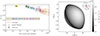 |
Fig. 6. Same as Fig. 5, but with free v sin i. The model was converged starting with the parameters from Table 4. The best fit model was with χVIS2 = 6.928. The free parameters were i = 58.3°, m = 28.0 M⊙, Ω = 301.5 deg, and Prot = 4.26 d. The fixed parameters were T = 27 000 K and γ = 25.9 km s−1. The derived parameters are v sin i = 277 km s−1, v = 325 km s−1, Requiv = 27.37 R⊙, Rpole = 22.29 R⊙, Requ = 33.61 R⊙, θequiv = 0.667 mas, θpole = 0.540 mas, and θequ = 0.814 mas. Again, the star is close to the critical rotation, but with an oblique orientation. This model better explains the visibilities along different baselines B/λ. The meaning of Ω is illustrated. |
3.2. Spectroscopy.
To constrain the radiative parameters, which were only assumed in the previous interferometric models, we used the spectra from CFHT. First, we checked the influence of i, i.e. v sin i, on synthetic line profiles, by computing forward models for the Balmer lines, Hγ, Hδ, Hε, Hζ, and Hη, which are not significantly influenced by the wind (Puebla et al. 2016). We used narrow ranges of wavelengths (±3, ±2.5, ±4, ±5, ±5) Å, respectively, in order to eliminate neighbouring lines. Also, we masked one remaining interstellar calcium line, 3968 Å, near Hε. In PHOEBE2, we set spe_method to ‘integrate’ and the interpolation to nearest-neighbour, to remain within the respective grid (Fig. 4) and prevent excessive extrapolation. Furthermore, we computed additional ATLAS synthetic spectra (Castelli & Kurucz 2003)5 for low values of log g and T, to describe critically rotating stars.
The resulting χSPE2 values for fixed v sin i are listed in Table 3 and for relaxed v sin i in Table 4. The χSPE2 contribution to the total χ2 is more than three orders of magnitude larger than χVIS2 because of the number of measurements. While χSPE2 and χVIS2 are the lowest for i = 14 deg in the models with fixed v sin i, there is a tension between spectra and visibilities for models with relaxed v sin i, which describes the interferometric data much better.
For comparison, we reconverged a model based only on spectroscopy, starting from the parameters with the lowest χSPE2 in Table 4 (bold); again with relaxed v sin i. The best-fit model is shown in Fig. 7, corresponding to χSPE2 = 1797. The free parameters and their resulting values were Prot = 4.535 d, T = 24915 K, and log g = 3.01, i = 21.0 deg. Other parameters were fixed and set according to interferometry. The derived projected velocity, v sin i = 111 km s−1, is substantially lower. A forward model based on parameters from interferometry, with higher v sin i, gives smeared lines, while the observed lines are sharper.
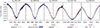 |
Fig. 7. Almost spherical model of ε Ori based on CFHT spectroscopy. Hydrogen Balmer lines were fitted using 1443 data points, excluding Hα and Hβ, which are ‘filled’ by wind-induced emission. An interstellar calcium 3968 Å for Hε was masked. The best fit resulted in χSPE2 = 1770. Free parameters were Prot = 4.551 d, T = 25 037 K, log g = 3.016, i = 21.40 deg, and γ = 25.00 km s−1. Other parameters were fixed and set according to interferometry. The derived parameters were v sin i = 111 km s−1 and v = 305 km s−1. The dotted lines show laboratory wavelengths, while the solid vertical lines indicate the Doppler-shifted line centres, corresponding to the resulting γ. The teal circles denote the points that contributed to χ2 with values greater than 10. This model explains reasonably well the Balmer lines, with a few systematics remaining in Hε, Hη, possibly due to different metal abundances. The temperature was constrained, and log g was slightly adjusted. However, due to the difference in inclination (i = 21 vs 62 deg), the interferometric model would become worse, with χVIS2 = 16.04. The fit of He I lines is given in Fig. C.5. |
3.3. Closure phase.
Unfortunately, even though closure phases are very useful to detect photocentre offsets, the observed amplitude from PIONIER seems to be too high (up to 4 deg) compared to any of our models. Even critically rotating stars, which have the largest differences of polar-to-equatorial temperatures (see Fig. C.4), exhibit synthetic amplitudes less than 0.1 deg (Fig. C.8). Nevertheless, taking into account only the signs and trends of argT3 versus λ, synthetic closure phases should change in the same sense as observed ones, which allowed us to resolve the Ω ambiguity (120 vs 300 deg) in Sect. 3.
3.4. SED.
As an independent check, we computed the PHOEBE2 model for the SED (using again the new module). As synthetic spectra, we used the absolute fluxes from the BSTAR, OSTAR, and ATLAS grids. The observed SED values were discussed in Sect. 2.4. We converged only the effective temperature Teff. Other parameters were fixed according to the model based on interferometry (from Fig. 6). The resulting value was Teff = 24 880 K, which is very close to the value inferred from the fitting of Balmer lines. Our model was in good agreement with the observed SED (see Fig. 8).
3.5. Compromise model.
Finally, we computed 2D χ2 maps to better understand the mutual relations between datasets (see Fig. 9). We always distinguished individual contributions to χ2, namely from interferometry (VIS), spectroscopy (SPE) and SED (SED). In each panel, we were changing only two parameters to get a regular grid, while other parameters are kept fixed. For mapping, we chose the period Prot from 4 d to 20 d with the step of 0.5 d versus the inclination i from 0 deg to 90 deg with the step of 5 deg. Alternatively, we chose the temperature, T, from 21 000 K to 30 000 K with the step of 500 K versus the mass, m, from 21 M⊙ to 32 M⊙ with the step of 0.5 M⊙. We recall here that m is always related to Requiv, as expressed in Eq. (7).
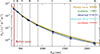 |
Fig. 8. SED model of ε Ori based on data from the Hvar Observatory and Vizier: the monochromatic flux, Fλ, vs wavelength, λ. The best-fit value was χSED2 = 52 with the following parameters: Teff = 24 654 K (fitted), d = 384 pc (fixed), M = 28.43 M⊙ (fixed), and R = 27.45 R⊙ (derived); other parameters were fixed and set according to interferometry. This model served as an independent verification of the temperature from the spectroscopic model. |
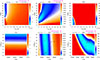 |
Fig. 9. Maps of χ2 for the ε Ori model. We performed 2D mapping of χ2 across different datasets: squared visibilities (VIS), spectral lines of Balmer series (SPE), and spectral energy distribution (SED). We systematically varied two parameters to create a regular grid (Prot vs i in the first row, T vs m in the second row). The remaining parameters were held fixed. The colour scale was adjusted as follows: cyan representing the best fit for a given dataset, blue, the acceptable fits, white, the poor fits, orange, the unacceptable fits, and red, the forbidden regions. In the first row, the fixed parameters are those resulting from the best fit of interferometric data in Fig. 6: d, m, and Ω; other fixed parameters are T = 25 000 K, log g = 3.011, and γ = 25.9 km s−1. The dependent parameters were Requiv and v sin i. In the second row, we set Prot and i according to the best fit in the first row. The individual panels, from the upper left, are as follows: I) the VIS dataset shows a preference for a critically rotating star and i around 45 deg; II) the SPE dataset (H lines) shows a preference for a fast-rotating star, Prot = 5 d, i = 25 deg. The correlation between Prot and i is due to rotation and v sin i; III) the SED dataset also allows a critically or fast-rotating star for i close to 20 deg. However, it is possible to re-fit T, R, or d to achieve improved SED fits in other regions of the parameter space; IV) the VIS dataset shows a flat dependence on temperature and the preferred mass; V) the SPE dataset for H lines demonstrates a weak correlation between T and m, the best fit of T is around 25 000 K; and VI) the SED dataset is strongly correlated between T and m due to the Stefan–Boltzmann law and Eq. (7). The crosses indicate the models from Tables 3 and 4. |
The VIS maps with squared visibility measurements show a preference for a critically rotating, oblate star, seen at an oblique angle (40 to 60 deg). On the other hand, there is a negligible dependence on temperature. A higher mass (28–30 M⊙) is preferred, but this is certainly correlated with the distance via Eq. (8).
The SPE maps with Balmer lines demonstrate that only lower inclinations can appropriately fit the depth and width of spectral lines. There is a weak correlation between the mass and temperature, indicating the appropriate temperature is around 25 000 K, while the mass is not well-constrained.
The SPE maps based on He I lines (Fig. 10) are quite similar. Although there is a correlation of good fits between i and Prot, we see a possible solution for a fast-rotating star, with a similar inclination to that derived from the Balmer lines. Again, the mass and temperature are weakly correlated, indicating the temperature 25 000 K. We note that the fits around 28 000 K resulted in poorer line depths. The SED maps are, of course, strongly influenced by the fixed temperature and mass, but they do show good solutions for a critically rotating star, with a similar inclination as for spectra. The mass and temperature are strongly correlated.
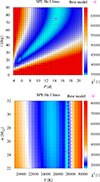 |
Fig. 10. Same as Fig. 9, but for the spectroscopic dataset based on He I lines. Top: SED dataset for He I lines exhibits results very similar to spectroscopy based on Balmer lines. The higher Prot and i values are excluded because of other datasets. Bottom: SED dataset for He I lines, indicating two possible solutions at T = 25 000 K or 27 500 K, due to systematic offsets in some lines. The model with T = 25 000 K fits the depths of He I lines better. The map also shows no preference for mass. |
We conclude that the inclination is the only uncertain parameter, for which the results differ according to interferometry (40 to 60 deg) versus spectroscopy (10 to 30 deg). Other parameters correspond to all three kinds of observations. As a compromise, we prefer the value around 40 deg, which partly explains both the interferometry and the spectroscopy. The resulting parameters of ε Ori are summarised in Table 5.
Resulting parameters of ε Ori based on a compromise among interferometry, spectroscopy, and SED.
3.6. Distance.
Finally, we tested distances of 350 pc and 420 pc (i.e. lower and upper limits from Sect. 2.5). We adjusted parameters of ε Ori using the constraints, Eqs. (6)–(8), in particular, m, Prot, Requiv, and Teff, so that these alternative models are also close to the respective datasets (VIS, SPE, and SED). According to χ2 maps similar to Fig. 9, the first row (Prot vs i) remains essentially unchanged, which would correspond to a poorly constrained distance. However, the second row (Teff, m) shows that these alternative models exhibit even larger tension between individual datasets (see Figs. C.6 and C.7). We thus conclude that there is no improvement and the nominal distance of 384 pc is still the preferred one.
4. Discussion
Our interferometry of ε Ori can be compared to Abeysekara et al. (2020), who performed intensity interferometry in B band. Their limb-darkened angular diameter, θLD = (0.660 ± 0.018) mas, is in perfect agreement with our measurements in H band (Table 5). Moreover, for their baseline T1-T4 (Abeysekara et al. 2020, Fig. 2, u-direction, east-west), approximately corresponding to our baseline A0-J6, their observations of V2 are above their spherical model, indicating a shorter angular size in that direction, which agrees with our non-spherical shape. Our model is also consistent with seminal papers Hanbury-Brown et al. (1974), even though their value of θ = (0.69 ± 0.04) mas was determined using only two baselines, and Code et al. (1976), reporting the bolometric flux of Fobs = (60.2 ± 5.4)⋅10−9 W m−2 and the effective temperature of T = (24 820 ± 920) K. However, as discussed in Sect. 3, the observed closure phases are high (up to 4 deg) compared to our model. This raises the question of what might have been missing in our model.
4.1. Possible binarity.
Such a modest amplitude in closure phases indicates a flux asymmetry with low contrast, up to 4° = 0.07 rad = 7%, in the Johnson:H passband. For this estimate, we assumed a maximally asymmetric object (i.e. a binary) and used the following closure phase approximation,  , where F1, F2 denote the fluxes of the two stars and ϕ the angular scale. Based on this, we estimated the mass of the companion, assuming that it is in the main sequence, up to ∼12 M⊙. To explain the observed dependence on B/λ, the angular scale should be of the order of 0.5 mas, corresponding to ∼40 R⊙. From this, we estimated the orbital period,
  , assuming the total mass ∼30 M⊙; namely, of the same order as the primary. The RV amplitudes for the primary and secondary are of the order of a hundred km s−1, but these could be suppressed by orbit orientation (e.g. for i = 5°, 15 km s−1). In the dataset of Thompson & Morrison (2013), there are RV variations of this order observed in the He I 5876 Å line. However, they are not persistent, and they cannot be phased with a fixed period. Only for one season, Thompson & Morrison (2013) reported a period of about 5 d. In the context of our model, this could correspond to the rotation period of the primary or (even more likely) to the variability of circumstellar material. More information on RV changes are given in Appendix B.
4.2. Wind.
Another asymmetry could be related to wind (Puebla et al. 2016), if the material expelled from ε Ori is not evenly distributed, but concentrated in relatively dense clumps. This phenomenon is especially relevant for hot, massive stars such as B supergiants, O-type stars, or Wolf-Rayet (WR) stars (Puls et al. 2008; Krtička et al. 2021). It is only when clumps are locally optically thick in the Johnson:H passband that they contribute to the respective continuum flux and the closure phase signal observed by PIONIER. Otherwise, wind is observed in the Hα line (Fig. 11), which is highly variable and exhibits a range of morphologies, from a classical P Cygni profile, an inverse P Cygni profile, double emission, to pure emission (see also Thompson & Morrison 2013, Fig. 1). Because of the variability in terms of Hα as well as the intense stellar wind and associated mass loss, we should be cautious when considering ε Ori as a standard for B-type stars (Negueruela et al. 2024).
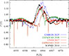 |
Fig. 11. Spectroscopy of ε Ori showing the Hα line profile that is highly variable and can be in several morphologies, like P Cygni profile, inverse P Cygni profile, double emission, or pure emission (Thompson & Morrison 2013). It implies an intense wind (e.g. Puebla et al. 2016) or a decretion disk fed by mass loss from the star. This variable line was not used in our modelling. |
4.3. Disk.
An additional asymmetry might be produced by an unresolved disk, fed by mass loss from the star and partially eclipsed by the star. If this is the source of the double emission sometimes observed in the wings of Hα (Fig. 11), the redshift and the blueshift, Δλ ≃ 6 Å, are interpreted as rotation, Δv = Δλ/λ c = 274 km s−1. This is surprisingly similar to the projected velocity v sin i in our models of ε Ori. Finally, if the star is close to critical rotation, as indicated by the PIONIER observations, we naturally expect an ongoing outflow from the equator.
4.4. Pulsations.
Moreover, ε Ori is close to the β Cep instability region (Paxton et al. 2015) for low-order modes, ℓ = 0, 1, 2 (see Fig. 12). Photometric observations of ε Ori seem to be compatible with typical periods ranging from 0.1 to 0.6 d, and the amplitudes ∼0.1 mag for β Cep variables (Lesh & Aizenman 1978). Such pulsations can enhance mass loss, especially if the star is rotating near its critical velocity. On the other hand, the periodograms for BRITE light curves or for RVs do not exhibit distinct peaks (Krtička & Feldmeier 2018; Thompson & Morrison 2013), so their interpretation is stochastic, episodic activity due to mass loss.
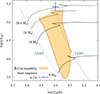 |
Fig. 12. HRD showing the position of ε Ori (blue) in comparison to the β-Cep instability region (ℓ = 0; orange), several evolutionary tracks (black) from Paxton et al. (2015), and evolutionary track for the mass of ε Ori computed by us using the MESA code. Note: the instability was computed only up to 24 M⊙, but the region most likely continues upwards, and the instability also occurs for the luminosity class Ia (log L/L⊙ ≥ 5.3). |
4.5. Stellar evolution.
If we, only for the moment, assumed a standard stellar evolution model for a 28.4 M⊙, rotating star, it would take ∼7.3 My to evolve from the zero-age main sequence (ZAMS) to B0Ia (Ekström et al. 2012; Paxton et al. 2013). This is about 25% longer than for a non-rotating star due to enhanced mixing and homogenised composition. For comparison, there are two groups of low-mass, young stellar objects (YSOs) observed in the vicinity of ε Ori, denoted ‘Orion C’ and ‘Orion D’ (Kounkel et al. 2018). Their ages span from approximately 0.3 to 5.5 My. They were classified as Class II or III, as some are still accreting and associated with translucent gas clouds (Briceño et al. 2005). This implies either that the stellar evolution for ε Ori was non-standard (e.g. with extreme mass loss) or the formation of low- and high-mass stars was not eodem loco et tempore Additionally, both the distance and the systemic velocity of ε Ori (384 pc and 8 km s−1, measured with respect to the local standard of rest) seem to be in the middle, namely, between Orion C and Orion D groups (Kounkel et al. 2018, Fig. 11). This relation might suggest that high-mass stars form either a bit earlier than low-mass stars or elsewhere (Sanhueza et al. 2017; Maud et al. 2018).
5. Conclusions
We obtained and calibrated VLTI/GRAVITY and PIONIER interferometric data for the brightest stars in Orion’s Belt, our closest star-forming region. In this first paper, we modelled the supergiant ε Ori based on VLTI/PIONIER visibility data, CFHT and CTIO spectra, and absolute fluxes. While the models based on interferometry indicate an oblate, critically rotating star, the models based on spectroscopy indicate a fast-rotating, less oblate star. The fast rotation might imply that ε Ori is a merger, for instance, similar to blue supergiants from Menon et al. (2024).
We also discussed the possibility of binarity, based on the asymmetry visible in closure phase data. However, due to the lack of consistent radial velocity variations, we excluded this binary model. We rather attributed the asymmetry to the clumped stellar wind or possibly to a decretion disk. To better constrain its properties, it is necessary to observe ε Ori with a spectro-interferometer such as CHARA/SPICA (Mourard et al. 2024), which is capable of scanning across the Hα line. In a forthcoming second paper, we will focus on the multiple stellar systems in Orion’s Belt.
Acknowledgments
A.O. was supported by GA UK grant no. 113224 of the Grant Agency of Charles University. M.B. was supported by GA ČR grant no. 25-16507S of the Czech Science Foundation. We thank other observers at the Hvar Observatory, Hrvoje Božić, Domagoj Ruždjak, and Davor Sudar for securing data for ε Ori. Thanks are due to an anonymous referee whose constructive feedback helped to improve the paper.
References
- Abbott, R., Abbott, T. D., Abraham, S., et al. 2021, ApJ, 913, L7 [NASA ADS] [CrossRef] [Google Scholar]
- Abeysekara, A. U., Benbow, W., Brill, A., et al. 2020, Nat. Astron., 4, 1164 [NASA ADS] [CrossRef] [Google Scholar]
- Allen, M. G., Ochsenbein, F., Derriere, S., et al. 2014, in Astronomical Data Analysis Software and Systems XXIII, eds. N. Manset, & P. Forshay, ASP Conf. Ser., 485, 219 [NASA ADS] [Google Scholar]
- Almeida, L. A., Sana, H., de Mink, S. E., et al. 2015, ApJ, 812, 102 [Google Scholar]
- Anderson, E., & Francis, C. 2012, Astron. Lett., 38, 331 [Google Scholar]
- Atri, P., Miller-Jones, J. C. A., Bahramian, A., et al. 2019, MNRAS, 489, 3116 [NASA ADS] [CrossRef] [Google Scholar]
- Baumann, M., Boch, T., Pineau, F. X., et al. 2022, in Astronomical Data Analysis Software and Systems XXX, eds. J. E. Ruiz, F. Pierfedereci, & P. Teuben, ASP Conf. Ser., 532, 7 [NASA ADS] [Google Scholar]
- Bessell, M. 1939, in Encyclopedia of Astronomy and Astrophysics, ed. P. Murdin [Google Scholar]
- Blanco, M., Demers, S., & Douglass, G. G. 1970, Photoelectric Catalogue - Magnitudes and Colors or Stars in the U, B, V and Uc, B, V Systems (Washington: United States Government Printing Office (USGPO)) [Google Scholar]
- Božić, H., & Harmanec, P. 2023, Highlights of a half century of the UBV photometry at Hvar [Google Scholar]
- Briceño, C., Calvet, N., Hernández, J., et al. 2005, AJ, 129, 907 [Google Scholar]
- Brož, M. 2017, ApJS, 230, 19 [Google Scholar]
- Brož, M., Prša, A., Conroy, K. E., & Abdul-Masih, M. 2025a, [arXiv:2506.20868] [Google Scholar]
- Brož, M., Prša, A., Conroy, K. E., Oplištilová, A., & Horvat, M. 2025b, [arXiv:2506.20865] [Google Scholar]
- Castelli, F., & Kurucz, R. L. 2003, in Modelling of Stellar Atmospheres, eds. N. Piskunov, W. W. Weiss, & D. F. Gray, IAU Symp., 210, A20 [Google Scholar]
- Clayton, D. D. 1983, Principles of Stellar Evolution and Nucleosynthesis (Chicago: University of Chicago Press) [Google Scholar]
- Code, A. D., Davis, J., Bless, R. C., & Brown, R. H. 1976, ApJ, 203, 417 [NASA ADS] [CrossRef] [Google Scholar]
- Conroy, K. E., Kochoska, A., Hey, D., et al. 2020, ApJS, 250, 34 [Google Scholar]
- Corcoran, M. F., Nichols, J. S., Pablo, H., et al. 2015, ApJ, 809, 132 [NASA ADS] [CrossRef] [Google Scholar]
- Cutri, R. M., Skrutskie, M. F., van Dyk, S., et al. 2003, VizieR Online Data Catalog, II/246 [Google Scholar]
- Cutri, R. M., Wright, E. L., & Conrow, T. 2012, VizieR Online Data Catalog, II/311 [Google Scholar]
- Ducati, J. R. 2002a, VizieR Online Data Catalog: Catalogue of Stellar Photometry in Johnson’s 11-color system., CDS/ADC Collection of Electronic Catalogues, 2237, 0 (2002) [Google Scholar]
- Ducati, J. R. 2002b, VizieR Online Data Catalog, II/237 [Google Scholar]
- Egan, M. P., Price, S. D., Kraemer, K. E., et al. 2003, VizieR Online Data Catalog, V/114 [Google Scholar]
- Eisenhauer, F., Perrin, G., Brandner, W., et al. 2011, The Messenger, 143, 16 [NASA ADS] [Google Scholar]
- Ekström, S., Georgy, C., Eggenberger, P., et al. 2012, A&A, 537, A146 [Google Scholar]
- Fan, H., Welty, D. E., York, D. G., et al. 2017, ApJ, 850, 194 [NASA ADS] [CrossRef] [Google Scholar]
- Freudling, W., Romaniello, M., Bramich, D. M., et al. 2013, A&A, 559, A96 [NASA ADS] [CrossRef] [EDP Sciences] [Google Scholar]
- Friedman, S. D., York, D. G., McCall, B. J., et al. 2011, ApJ, 727, 33 [NASA ADS] [CrossRef] [Google Scholar]
- Gaia Collaboration 2020, VizieR Online Data Catalog, I/350 [Google Scholar]
- Gaia Collaboration (Brown, A. G. A., et al.) 2021, A&A, 649, A1 [NASA ADS] [CrossRef] [EDP Sciences] [Google Scholar]
- Golay, M. 1974, Introduction to Astronomical Photometry (Dordrecht: Reidel) [Google Scholar]
- GRAVITY Collaboration (Abuter, R., et al.) 2017, A&A, 602, A94 [NASA ADS] [CrossRef] [EDP Sciences] [Google Scholar]
- Green, G. M., Schlafly, E., Zucker, C., Speagle, J. S., & Finkbeiner, D. 2019, ApJ, 887, 93 [NASA ADS] [CrossRef] [Google Scholar]
- Guinan, E. F., Mayer, P., Harmanec, P., et al. 2012, A&A, 546, A123 [NASA ADS] [CrossRef] [EDP Sciences] [Google Scholar]
- Hainich, R., Rühling, U., Todt, H., et al. 2014, A&A, 565, A27 [NASA ADS] [CrossRef] [EDP Sciences] [Google Scholar]
- Hanbury-Brown, R., Davis, J., & Allen, L. R. 1974, MNRAS, 167, 121 [NASA ADS] [CrossRef] [Google Scholar]
- Horvat, M., Conroy, K. E., Pablo, H., et al. 2018, ApJS, 237, 26 [Google Scholar]
- Houk, N., & Swift, C. 1999, Michigan Spectral Survey, 5 [Google Scholar]
- Hummel, C. A., White, N. M., Elias, N. M. I., Hajian, A. R., & Nordgren, T. E. 2000, ApJ, 540, L91 [NASA ADS] [CrossRef] [Google Scholar]
- Hummel, C. A., Rivinius, T., Nieva, M. F., et al. 2013, A&A, 554, A52 [NASA ADS] [CrossRef] [EDP Sciences] [Google Scholar]
- Ishihara, D., Onaka, T., Kataza, H., et al. 2010, A&A, 514, A1 [NASA ADS] [CrossRef] [EDP Sciences] [Google Scholar]
- Johnson, H. L., & Morgan, W. W. 1953, ApJ, 117, 313 [NASA ADS] [CrossRef] [Google Scholar]
- Jones, D., Conroy, K. E., Horvat, M., et al. 2020, ApJS, 247, 63 [Google Scholar]
- Kalari, V. M., Horch, E. P., Salinas, R., et al. 2022, ApJ, 935, 162 [NASA ADS] [CrossRef] [Google Scholar]
- Keller, S. C., Schmidt, B. P., Bessell, M. S., et al. 2007, PASA, 24, 1 [NASA ADS] [CrossRef] [Google Scholar]
- Kounkel, M., Covey, K., Suárez, G., et al. 2018, AJ, 156, 84 [NASA ADS] [CrossRef] [Google Scholar]
- Krtička, J., & Feldmeier, A. 2018, A&A, 617, A121 [NASA ADS] [CrossRef] [EDP Sciences] [Google Scholar]
- Krtička, J., Kubát, J., & Krtičková, I. 2021, A&A, 647, A28 [NASA ADS] [CrossRef] [EDP Sciences] [Google Scholar]
- Kuhn, M. A., Getman, K. V., Feigelson, E. D., et al. 2010, ApJ, 725, 2485 [NASA ADS] [CrossRef] [Google Scholar]
- Lanz, T., & Hubený, I. 2003, ApJS, 146, 417 [NASA ADS] [CrossRef] [Google Scholar]
- Lanz, T., & Hubený, I. 2007, ApJS, 169, 83 [CrossRef] [Google Scholar]
- Le Bouquin, J. B., Berger, J. P., Lazareff, B., et al. 2011, A&A, 535, A67 [NASA ADS] [CrossRef] [EDP Sciences] [Google Scholar]
- Lesh, J. R., & Aizenman, M. L. 1978, ARA&A, 16, 215 [NASA ADS] [CrossRef] [Google Scholar]
- Maíz Apellániz, J., Trigueros Páez, E., Negueruela, I., et al. 2019, A&A, 626, A20 [NASA ADS] [CrossRef] [EDP Sciences] [Google Scholar]
- Marchant, P., Pappas, K. M. W., Gallegos-Garcia, M., et al. 2021, A&A, 650, A107 [NASA ADS] [CrossRef] [EDP Sciences] [Google Scholar]
- Maud, L. T., Cesaroni, R., Kumar, M. S. N., et al. 2018, A&A, 620, A31 [NASA ADS] [CrossRef] [EDP Sciences] [Google Scholar]
- Menon, A., Ercolino, A., Urbaneja, M. A., et al. 2024, ApJ, 963, L42 [NASA ADS] [CrossRef] [Google Scholar]
- Mermilliod, J. C. 1994, Bulletin d’Information du Centre de Donnees Stellaires, 45, 3 [Google Scholar]
- Mourard, D., Meilland, A., Ibañez Bustos, R., et al. 2024, in Optical and Infrared Interferometry and Imaging IX, eds. J. Kammerer, S. Sallum, & J. Sanchez-Bermudez, SPIE Conf. Ser., 13095, 1309503 [Google Scholar]
- Negueruela, I., Simón-Díaz, S., de Burgos, A., Casasbuenas, A., & Beck, P. G. 2024, A&A, 690, A176 [NASA ADS] [CrossRef] [EDP Sciences] [Google Scholar]
- Nelder, J. A., & Mead, R. 1965, Comput. J., 7, 308 [Google Scholar]
- Neugebauer, G., Habing, H. J., van Duinen, R., et al. 1984, ApJ, 278, L1 [NASA ADS] [CrossRef] [Google Scholar]
- Nichols, J., Huenemoerder, D. P., Corcoran, M. F., et al. 2015, ApJ, 809, 133 [NASA ADS] [CrossRef] [Google Scholar]
- Oplištilová, A., Mayer, P., Harmanec, P., et al. 2023, A&A, 672, A31 [NASA ADS] [CrossRef] [EDP Sciences] [Google Scholar]
- Pablo, H., Richardson, N. D., Moffat, A. F. J., et al. 2015, ApJ, 809, 134 [NASA ADS] [CrossRef] [Google Scholar]
- Pauwels, T., Reggiani, M., Sana, H., Rainot, A., & Kratter, K. 2023, A&A, 678, A172 [NASA ADS] [CrossRef] [EDP Sciences] [Google Scholar]
- Paxton, B., Cantiello, M., Arras, P., et al. 2013, ApJS, 208, 4 [Google Scholar]
- Paxton, B., Marchant, P., Schwab, J., et al. 2015, ApJS, 220, 15 [Google Scholar]
- Perryman, M. A. C., Lindegren, L., Kovalevsky, J., et al. 1997, A&A, 323, L49 [Google Scholar]
- Pietrzyński, G., Graczyk, D., Gallenne, A., et al. 2019, Nature, 567, 200 [Google Scholar]
- Prša, A. 2011, PHOEBE Scientific Reference, Version 0.30, Villanova University, Department of Astronomy& Astrophysics, accessed: 2025-08-08 [Google Scholar]
- Prša, A., Conroy, K. E., Horvat, M., et al. 2016, ApJS, 227, 29 [Google Scholar]
- Puebla, R. E., Hillier, D. J., Zsargó, J., Cohen, D. H., & Leutenegger, M. A. 2016, MNRAS, 456, 2907 [NASA ADS] [CrossRef] [Google Scholar]
- Puls, J., Vink, J. S., & Najarro, F. 2008, A&A Rev., 16, 209 [NASA ADS] [CrossRef] [Google Scholar]
- Renzo, M., Hendriks, D. D., van Son, L. A. C., & Farmer, R. 2022, Res. Notes Am. Astron. Soc., 6, 25 [Google Scholar]
- Repolust, T., Puls, J., Hanson, M. M., Kudritzki, R. P., & Mokiem, M. R. 2005, A&A, 440, 261 [NASA ADS] [CrossRef] [EDP Sciences] [Google Scholar]
- Sana, H., Le Bouquin, J. B., Lacour, S., et al. 2014, ApJS, 215, 15 [Google Scholar]
- Sanhueza, P., Jackson, J. M., Zhang, Q., et al. 2017, ApJ, 841, 97 [Google Scholar]
- Schaefer, G. H., Hummel, C. A., Gies, D. R., et al. 2016, AJ, 152, 213 [NASA ADS] [CrossRef] [Google Scholar]
- Shenar, T., Oskinova, L., Hamann, W. R., et al. 2015, ApJ, 809, 135 [Google Scholar]
- Shenar, T., Sana, H., Mahy, L., et al. 2022, Nat. Astron., 6, 1085 [NASA ADS] [CrossRef] [Google Scholar]
- Sota, A., Maíz Apellániz, J., Morrell, N. I., et al. 2014, ApJS, 211, 10 [Google Scholar]
- Taniguchi, Y., Kajisawa, M., Kobayashi, M. A. R., et al. 2015, PASJ, 67, 104 [NASA ADS] [Google Scholar]
- Thompson, G. B., & Morrison, N. D. 2013, AJ, 145, 95 [Google Scholar]
- Tokovinin, A., Fischer, D. A., Bonati, M., et al. 2013, PASP, 125, 1336 [NASA ADS] [CrossRef] [Google Scholar]
- van Hamme, W. 1993, AJ, 106, 2096 [Google Scholar]
- van Leeuwen, F. 2007, A&A, 474, 653 [CrossRef] [EDP Sciences] [Google Scholar]
- von Zeipel, H. 1924, MNRAS, 84, 665 [NASA ADS] [CrossRef] [Google Scholar]
- Wilson, R. E., Van Hamme, W., & Terrell, D. 2010, ApJ, 723, 1469 [NASA ADS] [CrossRef] [Google Scholar]
- Wongwathanarat, A., Janka, H. T., & Müller, E. 2013, A&A, 552, A126 [NASA ADS] [CrossRef] [EDP Sciences] [Google Scholar]
Appendix A: Calibrator of ζ Ori: HIP 26108
The most challenging object for the calibration was ζ Ori because the diameter of its calibrator HIP 26108 in the pipeline database (GRAVI_FAINT_CALIBRATORS.fits) was clearly wrong, 1.77718 mas, and the squared visibility was greater than one in several wavelength intervals. Therefore, we determined the diameter of the calibrator based on the absolute flux from the photometric catalogues in the VizieR tool (Allen et al. 2014). We used the standard Johnson photometric system (Ducati 2002b) and measurements from Hipparcos (Anderson & Francis 2012), Gaia DR3 (Gaia Collaboration 2020), 2MASS (Cutri et al. 2003), WISE (Cutri et al. 2012), MSX (Egan et al. 2003), SkyMapper (Keller et al. 2007), Subaru/Suprime (Taniguchi et al. 2015), Akari (Ishihara et al. 2010), and IRAS (Neugebauer et al. 1984). The data covered the spectral range from 0.42 to 23.88 μm. In Table A.1, the SED of ε Ori is summarised.
For SED modelling, we used the reddening value EB − V = 0.014 mag, i.e. extinction AV = 0.0434 mag (Green et al. 2019) 6, and the parallax of (6.2 ± 0.1) mas from Gaia, corresponding to d = (161.1 ± 2.5) pc. Based on the spectral type K4III, we used the temperature T = 3 800 K and log g = 2.0. The fit with the lowest χ2 value (see Fig. A.1) led to the physical radius R = (33.52 ± 0.53) R⊙. We thus recalibrated ζ Ori using the calibrator’s angular diameter, θ = 2R/d = (1.935 ± 0.002) mas.
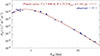 |
Fig. A.1. SED in terms of the monochromatic flux vs wavelength for the calibration star HIP 26108, which was used to determine the correct calibrator’s radius R = (33.52 ± 0.53) R⊙ and recalibrate the visibilities of ζ Ori. |
Absolute monochromatic fluxes for ε Ori.
Appendix B: Radial velocities
Thompson & Morrison (2013) measured RVs of the He I 6678 Å lines on 132 electronic spectra from the Ritter Observatory and found variations ranging from about −10 to +20 km s−1. In an effort to understand the nature of possible RV changes, we measured RVs of various spectral lines available in the high-resolution spectra at our disposal (CFHT, SOPHIE, and CTIO). The RVs were measured in reSPEFO, comparing direct and flipped line profiles on the computer screen. The zero point of the velocity scale was checked via measurements of a selection of telluric lines and also interstellar lines. The results of RV measurements are summarised in Table B.1. It is seen that the individual RVs from spectra taken during a particular observing night agree very well, but there are undoubtedly real RV changes from one observing season to another. We note, however, that the RVs of the He II lines of higher ionisation show little evidence of variability. This seems to contradict the presence of orbital motion in a putative binary system. The observed changes can be caused by some velocity fields in the stellar atmosphere and/or envelope. As Fig. C.1 illustrates, Hβ line shows variable asymmetry due to partial filling of one or another wing by the emission, which also seems to affect, to some extent, the He I 5876 and 6678 Å lines. A more systematic study of the nature of these changes seems desirable. At present, we conclude that the single-star models are preferable.
Individual radial velocities (in km s−1) measured in CFHT, SOPHIE, and CTIO electronic spectra.
Appendix C: Supplementary figures
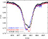 |
Fig. C.1. Hβ line exhibiting variable asymmetry due to partial emission filling in one of the wings. |
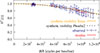 |
Fig. C.2. Spherical non-rotating model of ε Ori based VLTI/PIONIER observations. The squared visibility vs the projected baseline B/λ is plotted for two models, Xitau (Brož 2017) and Phoebe (Brož et al. 2025b). The resulting χVIS2 = 12.1 is the same in both cases. The number of degrees of freedom, ν = N − M = 35. The resulting parameters are m = 23.52 M⊙ (free), d = 384 pc (fixed), T = 27 000 K (fixed according to Puebla et al. 2016), log g = 3.0 (fixed according to Puebla et al. 2016), R = 25.40 R⊙ (derived), θ = 0.615 mas (derived). |
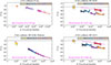 |
Fig. C.3. Examples of raw visibilities of the calibrators for ε, δ, ζ, and σ Ori and the corresponding Bessel functions with the calibrator’s diameters plotted for reference (magenta). Measurements are from nights: 20 November 2023, 22 November 2023, 8 January 2024, and 23 November 2023, respectively. Colours correspond to individual baselines. |
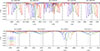 |
Fig. C.4. Synthetic He I and He II line profiles from our spectroscopic model, corresponding to selected triangles with given temperatures and RVs. They demonstrate where lines form in our model. For a fast-rotating star, the pole is substantially hotter than the equator. The central line (RV = 0) corresponds to the pole, other lines originate from the equator (RV ≠ 0). He I and He II lines form at different locations on a fast or critically rotating star due to strong temperature gradients. He I lines have the lowest intensity on the poles, while He II lines have the highest intensity at the poles. He I lines are less intense at the pole, while He II lines are less intense on the equator. The grey points indicate the He I lines for clarity. |
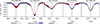 |
Fig. C.5. Same as Fig. 7, but for He I lines. The best-fit spectroscopic model still exhibits systematics (in particular, 4009 and 4026 Å lines). None of these are easy to correct, e.g. by changing T, log g, or metallicity; see also Puebla et al. (2016). |
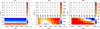 |
Fig. C.6. Same as the second row of Fig. 9, but for the distance of 350 pc, computed on a somewhat coarser grid. Blank regions mark combinations where R > Rcrit; crosses indicate grid points exceeding this limit. PHOEBE2 model also fails very near the critical boundary, which we explored with finer grids. |
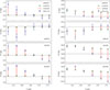 |
Fig. C.8. Model of ε Ori showing a forward computation of the closure phases with fixed parameters from the visibility model (Fig. 6). The observed closure phases reach up to nearly 4 deg, while the synthetic ones are at most 0.15 deg. If we recalibrate the observed closure phases (left column) by multiplying them by scaling factors 1/40, 1/6, 1/100, and 1/18, respectively for each of the triple baselines (right column), we see similar trends in the observed and synthetic closure phases, arg T3 vs B/λ. We used this asymmetry of the flux to set the orientation of the star’s equator, as seen by the observer, Ω (favouring 300 deg over 120 deg). |
All Tables
Epochs of interferometric observations and uniform-disk diameters (UDD) of calibrators.
Grid of almost spherical models for ε Ori assuming a fixed value of v sin i = 70 km s−1.
Resulting parameters of ε Ori based on a compromise among interferometry, spectroscopy, and SED.
Individual radial velocities (in km s−1) measured in CFHT, SOPHIE, and CTIO electronic spectra.
All Figures
|
Fig. 1. Coverage for interferometric measurements showing the squared visibility V2 vs baselines (u,v) ≡ B/λ in cycles per baseline. Individual panels show four stars in Orion’s Belt (ζ, σ, ε, and δ Ori). For each star, all nights are plotted. Colours correspond to visibility values. |
| In the text | |
|
Fig. 2. Examples of reduced squared visibilities, V2, of the science targets, ε, δ, ζ, and σ Ori. Measurements are from nights: 20 November 2023, 22 November 2023, 8 January 2024, and 23 November 2023, respectively. Science targets are with obvious signals from companions. For the single star ε Ori, the signal suggests an elongated or non-spherical shape, unlike the calibrator ζ Lep, which exhibits a perfectly spherical shape. Colours correspond to individual baselines. The squared visibilities of calibrators are in Fig. C.3. |
| In the text | |
|
Fig. 3. Comparison of DIBs’ intensities for ε Ori and stars which are close on the sky (HD 37140 and HD 36628). The most distant star has the deepest DIBs, while the star with the lowest distance has very weak DIBs. The spectrum of ε Ori also shows weak DIBs, which suggests its distance is lower than 420 pc. The spectra were taken from public archives of CFHT and ESO. |
| In the text | |
|
Fig. 4. Grids of synthetic spectra BSTAR and OSTAR (Lanz & Hubený 2003, 2007) used in our spectroscopic models. Each spectrum is parametrised by log g and T. To describe also critically rotating stars (cf. green points), it was necessary to compute additional ATLAS spectra (Castelli & Kurucz 2003) for low values of log g and T. |
| In the text | |
|
Fig. 5. Almost spherical model of ε Ori based on PIONIER observations in H-band with fixed v sin i (Puebla et al. 2016). Left: Squared visibility vs projected baseline B/λ. Right: Corresponding triangular mesh with the passband intensities (greyscale). The model was converged starting with the parameters from Table 3 (bold line). The best-fit was with χVIS2 = 11.23. The free parameters were i = 13.6 deg, m = 20.3 M⊙, Ω = 293.7 deg, Prot = 4.01 d. The fixed parameters were v sin i = 70 km s−1, T = 25 000 K, γ = 25.9 km s−1 and the derived parameters were v = 298 km s−1, Requiv = 22.43 R⊙(derived), Rpole = 22.29 R⊙ (derived), Requ = 22.46 R⊙ (derived), θequiv = 0.543 mas. The star is close to critical rotation and has an almost pole-on orientation in order to decrease projected rotation (cf. v sin i). |
| In the text | |
|
Fig. 6. Same as Fig. 5, but with free v sin i. The model was converged starting with the parameters from Table 4. The best fit model was with χVIS2 = 6.928. The free parameters were i = 58.3°, m = 28.0 M⊙, Ω = 301.5 deg, and Prot = 4.26 d. The fixed parameters were T = 27 000 K and γ = 25.9 km s−1. The derived parameters are v sin i = 277 km s−1, v = 325 km s−1, Requiv = 27.37 R⊙, Rpole = 22.29 R⊙, Requ = 33.61 R⊙, θequiv = 0.667 mas, θpole = 0.540 mas, and θequ = 0.814 mas. Again, the star is close to the critical rotation, but with an oblique orientation. This model better explains the visibilities along different baselines B/λ. The meaning of Ω is illustrated. |
| In the text | |
|
Fig. 7. Almost spherical model of ε Ori based on CFHT spectroscopy. Hydrogen Balmer lines were fitted using 1443 data points, excluding Hα and Hβ, which are ‘filled’ by wind-induced emission. An interstellar calcium 3968 Å for Hε was masked. The best fit resulted in χSPE2 = 1770. Free parameters were Prot = 4.551 d, T = 25 037 K, log g = 3.016, i = 21.40 deg, and γ = 25.00 km s−1. Other parameters were fixed and set according to interferometry. The derived parameters were v sin i = 111 km s−1 and v = 305 km s−1. The dotted lines show laboratory wavelengths, while the solid vertical lines indicate the Doppler-shifted line centres, corresponding to the resulting γ. The teal circles denote the points that contributed to χ2 with values greater than 10. This model explains reasonably well the Balmer lines, with a few systematics remaining in Hε, Hη, possibly due to different metal abundances. The temperature was constrained, and log g was slightly adjusted. However, due to the difference in inclination (i = 21 vs 62 deg), the interferometric model would become worse, with χVIS2 = 16.04. The fit of He I lines is given in Fig. C.5. |
| In the text | |
|
Fig. 8. SED model of ε Ori based on data from the Hvar Observatory and Vizier: the monochromatic flux, Fλ, vs wavelength, λ. The best-fit value was χSED2 = 52 with the following parameters: Teff = 24 654 K (fitted), d = 384 pc (fixed), M = 28.43 M⊙ (fixed), and R = 27.45 R⊙ (derived); other parameters were fixed and set according to interferometry. This model served as an independent verification of the temperature from the spectroscopic model. |
| In the text | |
|
Fig. 9. Maps of χ2 for the ε Ori model. We performed 2D mapping of χ2 across different datasets: squared visibilities (VIS), spectral lines of Balmer series (SPE), and spectral energy distribution (SED). We systematically varied two parameters to create a regular grid (Prot vs i in the first row, T vs m in the second row). The remaining parameters were held fixed. The colour scale was adjusted as follows: cyan representing the best fit for a given dataset, blue, the acceptable fits, white, the poor fits, orange, the unacceptable fits, and red, the forbidden regions. In the first row, the fixed parameters are those resulting from the best fit of interferometric data in Fig. 6: d, m, and Ω; other fixed parameters are T = 25 000 K, log g = 3.011, and γ = 25.9 km s−1. The dependent parameters were Requiv and v sin i. In the second row, we set Prot and i according to the best fit in the first row. The individual panels, from the upper left, are as follows: I) the VIS dataset shows a preference for a critically rotating star and i around 45 deg; II) the SPE dataset (H lines) shows a preference for a fast-rotating star, Prot = 5 d, i = 25 deg. The correlation between Prot and i is due to rotation and v sin i; III) the SED dataset also allows a critically or fast-rotating star for i close to 20 deg. However, it is possible to re-fit T, R, or d to achieve improved SED fits in other regions of the parameter space; IV) the VIS dataset shows a flat dependence on temperature and the preferred mass; V) the SPE dataset for H lines demonstrates a weak correlation between T and m, the best fit of T is around 25 000 K; and VI) the SED dataset is strongly correlated between T and m due to the Stefan–Boltzmann law and Eq. (7). The crosses indicate the models from Tables 3 and 4. |
| In the text | |
|
Fig. 10. Same as Fig. 9, but for the spectroscopic dataset based on He I lines. Top: SED dataset for He I lines exhibits results very similar to spectroscopy based on Balmer lines. The higher Prot and i values are excluded because of other datasets. Bottom: SED dataset for He I lines, indicating two possible solutions at T = 25 000 K or 27 500 K, due to systematic offsets in some lines. The model with T = 25 000 K fits the depths of He I lines better. The map also shows no preference for mass. |
| In the text | |
|
Fig. 11. Spectroscopy of ε Ori showing the Hα line profile that is highly variable and can be in several morphologies, like P Cygni profile, inverse P Cygni profile, double emission, or pure emission (Thompson & Morrison 2013). It implies an intense wind (e.g. Puebla et al. 2016) or a decretion disk fed by mass loss from the star. This variable line was not used in our modelling. |
| In the text | |
|
Fig. 12. HRD showing the position of ε Ori (blue) in comparison to the β-Cep instability region (ℓ = 0; orange), several evolutionary tracks (black) from Paxton et al. (2015), and evolutionary track for the mass of ε Ori computed by us using the MESA code. Note: the instability was computed only up to 24 M⊙, but the region most likely continues upwards, and the instability also occurs for the luminosity class Ia (log L/L⊙ ≥ 5.3). |
| In the text | |
|
Fig. A.1. SED in terms of the monochromatic flux vs wavelength for the calibration star HIP 26108, which was used to determine the correct calibrator’s radius R = (33.52 ± 0.53) R⊙ and recalibrate the visibilities of ζ Ori. |
| In the text | |
|
Fig. C.1. Hβ line exhibiting variable asymmetry due to partial emission filling in one of the wings. |
| In the text | |
|
Fig. C.2. Spherical non-rotating model of ε Ori based VLTI/PIONIER observations. The squared visibility vs the projected baseline B/λ is plotted for two models, Xitau (Brož 2017) and Phoebe (Brož et al. 2025b). The resulting χVIS2 = 12.1 is the same in both cases. The number of degrees of freedom, ν = N − M = 35. The resulting parameters are m = 23.52 M⊙ (free), d = 384 pc (fixed), T = 27 000 K (fixed according to Puebla et al. 2016), log g = 3.0 (fixed according to Puebla et al. 2016), R = 25.40 R⊙ (derived), θ = 0.615 mas (derived). |
| In the text | |
|
Fig. C.3. Examples of raw visibilities of the calibrators for ε, δ, ζ, and σ Ori and the corresponding Bessel functions with the calibrator’s diameters plotted for reference (magenta). Measurements are from nights: 20 November 2023, 22 November 2023, 8 January 2024, and 23 November 2023, respectively. Colours correspond to individual baselines. |
| In the text | |
|
Fig. C.4. Synthetic He I and He II line profiles from our spectroscopic model, corresponding to selected triangles with given temperatures and RVs. They demonstrate where lines form in our model. For a fast-rotating star, the pole is substantially hotter than the equator. The central line (RV = 0) corresponds to the pole, other lines originate from the equator (RV ≠ 0). He I and He II lines form at different locations on a fast or critically rotating star due to strong temperature gradients. He I lines have the lowest intensity on the poles, while He II lines have the highest intensity at the poles. He I lines are less intense at the pole, while He II lines are less intense on the equator. The grey points indicate the He I lines for clarity. |
| In the text | |
|
Fig. C.5. Same as Fig. 7, but for He I lines. The best-fit spectroscopic model still exhibits systematics (in particular, 4009 and 4026 Å lines). None of these are easy to correct, e.g. by changing T, log g, or metallicity; see also Puebla et al. (2016). |
| In the text | |
|
Fig. C.6. Same as the second row of Fig. 9, but for the distance of 350 pc, computed on a somewhat coarser grid. Blank regions mark combinations where R > Rcrit; crosses indicate grid points exceeding this limit. PHOEBE2 model also fails very near the critical boundary, which we explored with finer grids. |
| In the text | |
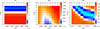 |
Fig. C.7. As Fig. C.6 but for the distance of 420 pc. |
| In the text | |
|
Fig. C.8. Model of ε Ori showing a forward computation of the closure phases with fixed parameters from the visibility model (Fig. 6). The observed closure phases reach up to nearly 4 deg, while the synthetic ones are at most 0.15 deg. If we recalibrate the observed closure phases (left column) by multiplying them by scaling factors 1/40, 1/6, 1/100, and 1/18, respectively for each of the triple baselines (right column), we see similar trends in the observed and synthetic closure phases, arg T3 vs B/λ. We used this asymmetry of the flux to set the orientation of the star’s equator, as seen by the observer, Ω (favouring 300 deg over 120 deg). |
| In the text | |
Current usage metrics show cumulative count of Article Views (full-text article views including HTML views, PDF and ePub downloads, according to the available data) and Abstracts Views on Vision4Press platform.
Data correspond to usage on the plateform after 2015. The current usage metrics is available 48-96 hours after online publication and is updated daily on week days.
Initial download of the metrics may take a while.