| Issue |
A&A
Volume 704, December 2025
|
|
|---|---|---|
| Article Number | A223 | |
| Number of page(s) | 19 | |
| Section | Planets, planetary systems, and small bodies | |
| DOI | https://doi.org/10.1051/0004-6361/202556553 | |
| Published online | 17 December 2025 | |
Knobs and dials of retrieving JWST transmission spectra
II. Impacts of pipeline-level differences on retrieval posteriors
1
Department of Astrophysics, University of Vienna,
Türkenschanzstrasse 17,
1180
Vienna,
Austria
2
Kapteyn Astronomical Institute, University of Groningen,
PO Box 800,
9700 AV
Groningen,
The Netherlands
3
Department of Physics and Astronomy, University College London,
Gower Street,
WC1E 6BT
London,
UK
4
Department of Meteorology and Geophysics, University of Vienna,
Josef-Holaubek-Platz 2,
Vienna,
Austria
★ Corresponding author: This email address is being protected from spambots. You need JavaScript enabled to view it.
Received:
23
July
2025
Accepted:
7
November
2025
Abstract
Context. Since the launch of the James Webb Space Telescope (JWST), observations of exoplanetary atmospheres have experienced a revolution in data quality. As atmospheric parameter inferences heavily depend on the underlying dataset, a re-evaluation of current methodologies is warranted to assess the reliability of these results.
Aims. We investigate the impact of variations in input spectra on atmospheric retrievals for the hot Jupiter WASP-39 b using JWST transit data. Specifically, we analyse the reliability of parameter estimation results from random perturbations of the underlying spectrum, and their sensitivity to the use of three transmission spectra derived from the same observational data.
Methods. Using the NIRSpec PRISM observation from a single transit of WASP-39 b, we performed retrievals with the TauREx framework. As an input baseline, we used a transmission spectrum derived in our work using the Eureka! data reduction pipeline. To investigate the reliability of these retrieval results, we analysed the behaviour of parameter posterior distributions under deviations of this spectrum. To mimic random noise, we performed a set of retrievals on scattered instances of the spectrum produced in this work. We compared this to differences resulting from retrievals based on existing spectra reduced from the same raw observation.
Results. Our analysis identifies three types of parameter posterior distributions: (1) stable, Gaussian distributions for species constrained across the entire spectrum (e.g. H2O and CO2); (2) uniform posteriors with upper bounds for species with weak constraints (e.g. CO and CH4); and (3) unstable, heavy-tailed posteriors for species constrained only by minor spectrum features (e.g. SO2 and C2H2). We find that other parameters, such as the planetary radius and pressure-temperature profile, are stable under spectral perturbations. Conclusions. Parameter posterior distributions are different for atmospheric retrievals performed on independently reduced transmission spectra derived from the same raw data. This makes a robust interpretation difficult, particularly for skewed distributions. Based on this, we advocate for the careful assessment and selection of credible interval sizes to reflect this.
Key words: methods: statistical / techniques: spectroscopic / planets and satellites: atmospheres / planets and satellites: composition
© The Authors 2025
 Open Access article, published by EDP Sciences, under the terms of the Creative Commons Attribution License (https://creativecommons.org/licenses/by/4.0), which permits unrestricted use, distribution, and reproduction in any medium, provided the original work is properly cited.
This article is published in open access under the Subscribe to Open model. This email address is being protected from spambots. You need JavaScript enabled to view it. to support open access publication.
1 Introduction
With the launch of the James Webb Space Telescope (JWST, Gardner et al. 2023), the frontier of exoplanetary sciences has been pushed forward significantly. Among the many advances that JWST has brought are observations of exoplanetary atmospheres of a quality far surpassing those previously available from other observatories. Together with the ever-increasing inventory of known exoplanets, these advancements are starting to enable the inference of population-level planetary parameters (Fu et al. 2025), as well as detailed studies of the atmospheres of individual exoplanets.
One of the most deeply studied exoplanets with JWST is WASP-39 b (Faedi et al. 2011), a Saturn-mass hot Jupiter selected for the early release science (ERS) programme for transiting exoplanets. WASP-39 b has been observed with all four instruments of JWST, which has led to the detection of several atmospheric trace species, such as CO2, H2O, Na, and K (e.g. Ahrer et al. 2023; Alderson et al. 2023; Rustamkulov et al. 2023; Feinstein et al. 2023). It has also led to the first detection of SO2 in the atmosphere of an exoplanet, a product of photochemical processes (Alderson et al. 2023; Tsai et al. 2023; Powell et al. 2024), marking one of the early milestones in exoplan-etary sciences achieved with JWST. However, putting precise constraints on identified atmospheric characteristics has proven to be difficult, as the results of characterisation techniques are sensitive to model setup assumptions and the steps taken in the data reduction process (e.g. Constantinou et al. 2023; Lueber et al. 2024). The jump in data quality with JWST also poses new challenges, which need to be addressed to appropriately adjust the methodology used to infer the atmospheric properties of exoplanets.
The most prevalent technique used to characterise exoplan-etary atmospheres is called atmospheric retrieval. This method has been used to infer atmospheric properties from data of different observational methods, including transmission, emission, and phase curve spectroscopy, as well as direct imaging. We refer readers to Madhusudhan (2019) or Barstow & Heng (2020), for instance, for comprehensive reviews on this topic. With the increased spectral resolution, precision, and wavelength coverage of JWST, the assumptions and approaches used in atmospheric retrievals need to be adjusted in a manner that reflects the increased information content in these state-of-the-art observations.
Atmospheric retrieval is a data-driven inverse modelling technique, and the parameters inferred from it depend on two main factors. One of these is the forward model used to represent the atmospheric observation. In atmospheric retrievals, these models are commonly constructed as 1D vertical slices of the probed atmospheric region, possibly under-representing the inherent 3D nature of a planetary atmosphere (Blecic et al. 2017; Caldas et al. 2019; Espinoza & Jones 2021; Pluriel et al. 2022). Adjusting forward models to properly reflect the information contained in current observational data is a key factor to avoid characterisation biases from oversimplified assumptions (e.g. Changeat et al. 2019; Al-Refaie et al. 2022; Schleich et al. 2024).
The other factor is the underlying observational data on which the parameter estimates of the atmospheric forward model are optimised. Assumptions and techniques applied at different stages of the data reduction process can influence the resulting atmospheric spectrum, propagating into the results of atmospheric characterisation efforts. At the highest level, combining atmospheric spectra from multiple instruments introduces the problem of agreement between mean transit depths. The treatment of these potential offsets between spectra of the same planet can propagate into different conclusions about its atmospheric nature (Madhusudhan et al. 2023; Edwards et al. 2024). When considering individual instruments, assumptions such as temporal and chromatic binning (Morello et al. 2022; Davey et al. 2025), as well as the characterisation of stellar limb darkening (Morello et al. 2017; Keers et al. 2024), act as another source of bias influencing the reliability of atmospheric characterisation results. At the lowest level, individual data reduction pipelines and techniques could introduce disagreements into derived atmospheric spectra, which propagate into atmospheric characterisation results through discrepancies in estimated parameter values (e.g. Mugnai et al. 2024). Being aware of and accounting for all of these sources of bias is imperative when maximising the potential for atmospheric characterisation that JWST is providing to us.
Our goal for this work was to investigate how random and systematic differences in instances of a transmission spectrum propagate into the results of atmospheric retrievals. Firstly, we performed end-to-end data reduction of the NIRSpec PRISM observation of the hot Jupiter WASP-39 b using the open-source pipeline Eureka! (Bell et al. 2022) to derive a transmission spectrum. We performed forward model tuning on the basis of this spectrum and investigated the impact of random data perturbations by applying standardised atmospheric retrievals to scattered instances of this spectrum. We also analysed the results of the atmospheric retrieval achieved on two more transmission spectra of WASP-39 b. These spectra were derived from the same underlying data used in our work, a single-transit observation with the NIRSpec PRISM instrument configuration. Next to the spectrum produced for this work, we considered the Eureka!-derived transmission spectrum presented in Rustamkulov et al. (2023), the first reported transmission spectrum considering the full wavelength range of NIRSpec PRISM and treating partial saturation. Additionally, we used the transmission spectrum presented in Carter & May et al. (2024), which was produced in an effort to homogenise the analysis of all available nearinfrared observations of WASP-39 b. We note that Carter & May et al. (2024) adopted the spectral time series data from Rustamkulov et al. (2023), which was reduced with the FIREFLy pipeline.
System parameters for WASP-39.
2 Observational data
WASP-39 b is a Saturn-mass hot Jupiter (Mp = 0.281 MJ and Rp = 1.279 RJ) orbiting a late G-type star at a period of approximately 4d (Faedi et al. 2011, see Table 1). It is part of the JWST early release science (ERS) programme for transiting exoplanets (PID: 1366, PI: N. Batalha, Co-PIs: J. Bean and K. Stevenson) as a target for transmission spectroscopy. The JWST panchromatic transmission spectroscopy observations of this target include transits observed with all near-infrared (NIR) instruments of JWST. A follow-up observation stipulated by the identification of SO2 in the atmosphere of WASP-39 b (Alderson et al. 2023; Tsai et al. 2023) also added a mid-infrared (MIR) transmission spectrum (Powell et al. 2024). This makes the panchromatic transmission spectrum of WASP-39 b one of the most extensive ones produced by JWST so far.
The dataset we analyse in this work is the singular transit NIRSpec PRISM observation of WASP-39 b, taken on 10 July 2022 (14:05 - 23:38 UT). The raw observational data (noncalibrated Stage 1b, or .uncal-files) were queried from the Mikulski Archive for Space Telescopes (MAST).
2.1 Data reduction
We use the open-source pipeline Eureka! (Bell et al. 2022) to perform end-to-end data reduction on the raw JWST data products. Eureka! acts both as a wrapper for the official jwst pipeline (Bushouse et al. 2024) in its first stages and as a framework to perform light-curve fitting. Eureka! is highly modular, supporting the fine-tuning of data reduction steps to ensure optimal precision in the produced data products. We refer to Appendix D for a detailed description of the data reduction steps taken in this work, and summarise the individual stages below.
The first three stages of Eureka! are concerned with detector-level data processing, as well as calibration and reduction. These stages transform the raw observational data into reduced dynamic light-curves. We perform stages 1 and 2 with mainly default assumptions. For the jump_rejection step in stage 1, we choose a threshold of 10 σ to counteract excessive pixel flagging connected to the low number of groups in each integration (Rustamkulov et al. 2023). To mitigate the effects of 1/f-noise, we perform group-level background subtraction (GLBS) in this stage. The refpix step is omitted in this stage, as there are no reference pixels on the subarray used for this observation (Birkmann et al. 2022). We also omit the flat_field step in stage 2, which did not work as intended at the time of data reduction (e.g. Alderson et al. 2023; Sarkar et al. 2024). In stage 3, we restrict the extracted detector region to x > 160 based on a conservative saturation threshold of 60%. We perform the spectral extraction with a combination of (6,9) for the pixel-width of the aperture and background, respectively.
The final three stages of Eureka! process the dynamic light-curve data and perform light-curve fitting to extract a transmission spectrum. In stage 4, we extract the spectroscopic light-curves at a detector-pixel level. We flag individual channels with a noise level higher than a factor of 1.75 compared to noise-budget simulations as deviations, excluding them from further analysis. The light-curve fitting in stage 5 is done using the batman Python package (Kreidberg 2015). We fit a combined astrophysical and systematics model to each spectroscopic, as well as the integrated white light-curve. We use pre-calculated limb-darkening coefficients from the ExoTiC-LD Python package (Grant & Wakeford 2022). Lastly, we bin the transmission spectrum into fixed groups of 3 pixels. This accounts for the typical instrument resolution element size of 2.2 pixels for NIRSpec (Jakobsen et al. 2022). We show the final transmission spectrum produced in this work in Fig. 1. For clarity, we refer to the transmission spectrum produced in this work as SP-TW (‘Spectrum -This work’) from here onwards.
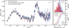 |
Fig. 1 Comparison of transmission spectra used in this work. Data associated with the spectrum produced in this work (SP-TW) are shown in black, while data associated with Rustamkulov et al. (2023) (RU-23) and Carter & May et al. (2024) (CA-24) are shown in red and blue, respectively. (a) Transmission spectra, showing wavelength (in μm) on the x-axis and transit depth (in %) on the y-axis. (b) Residual distribution of RU-23 and CA-24, normalised to the transit depth uncertainty of SP-TW. For display purposes, the residuals are binned in steps of 0.5 σsp-TW. (c) Empirical cumulative distribution functions (eCDF) for the residuals of RU-23 and CA-24. The values of a one-sample K-S test for a standard normal distribution are given in the legend of the figure. In (b) and (c), the black dashed line represents the PDF and CDF of N(0,1), respectively. |
2.2 Panchromatic perturbation of the spectrum
The results of atmospheric retrievals are anchored to the underlying dataset used in the inference process. As these data guide the parameter estimation, in a Bayesian inference framework they are assumed to be the true state. However, the parameter estimates derived from a forward model have a non-uniform dependence on the data points of a transmission spectrum.
One method used to judge the importance of individual spectral data points in the parameter estimation process is a leave-one-out cross-validation (LOO-CV) technique computing the expected log pointwise predictive density (elpdLOO). LOO-CV works by fitting a given model to a dataset with one data point removed (Gelman et al. 2014). In the analysis of pre-JWST data, this method requires of the order of several tens of retrievals, each time performing an atmospheric retrieval while excluding an individual spectral data point. However, for current state-of-the-art data, this requirement would be increased by several orders of magnitude, accounting for the increased resolution and wavelength coverage of JWST. Current applications of LOO-CV make use of the PSIS approximation (Vehtari et al. 2017) to avoid this computational boundary (e.g. Welbanks et al. 2023; Murphy et al. 2025).
Additionally, atmospheric absorbers produce correlated signals within an atmospheric spectrum. A comprehensive investigation of the posterior dependence on the underlying spectrum would also require a validation analysis under all possible combinations of excluded data points. This would be computationally extremely expensive when considering datasets as provided by JWST, with hundreds or thousands of individual data points.
As an initial test of the stability of our retrieval results to perturbations of the underlying data, we therefore opt to produce fully scattered instances of SP-TW (shown in Fig. 1, which we consider to be true). We successively create randomised instances of SP-TW by drawing new transit depth values using a normal distribution N(μtd,λ, σ2td,λ), where μtd,λ and σtd,λ represent the baseline transit depth mean and standard deviation, respectively. We attach the existing transit depth uncertainties, σtd,λ, to these new transit depth values to create scattered instances of SP-TW. While this method is not sensitive to possible correlated noise, it provides insight into the stability of the posterior distributions under deviations following a normal distribution. Considering perturbations from data reduction assumptions, we interpret these scattered instances as deviations following random noise. These spectra are used as input data for the standardised atmospheric retrieval analysis described in Sect. 4.2.
2.3 Existing transmission spectra
While we present our own data reduction results for the transmission spectrum of WASP-39 b from a NIRSpec PRISM observation, previous analyses of the same data exist as well. Using Bayesian inference to estimate model parameters is inherently dependent on the underlying dataset. As recently shown by Mugnai et al. (2024) and Edwards et al. (2024), data-reduction-based variations in transmission spectra from Hubble Space Telescope (HST) observations can affect the derived exoplanet atmospheric properties. This leads to diverging conclusions about individual-and population-level characterisation results. We are conscious of this potential biasing effect when only considering the transmission spectrum produced in this work. We therefore investigate the results of applying the atmospheric retrieval setup described above to existing transmission spectra derived from the same underlying observational data.
Rustamkulov et al. (2023) presented a reduction of the NIR-Spec PRISM observation of WASP-39 b with a specific focus on recovering the signal in the saturated region of the detector. Out of the four different pipeline results presented in their work, we use the Eureka!-based data reduction (referred to as RU-23 from here onwards)1. Compared to the data reduction performed in this work (as described in Appendix D), RU-23 was derived with several different assumptions. A detailed description of these data reduction steps can be found in the ‘Methods’ section of Rustamkulov et al. (2023), but the main differences are listed in Table D.2.
Additionally, a recent study by Carter & May et al. (2024) reanalysed the full range of observations taken with the nearinfrared instruments of JWST as part of the ERS programme. From the results presented in their work, we use the NIRSpec PRISM transmission spectrum at native instrument resolution, derived with fixed limb-darkening coefficients (referred to as CA-24 from here onwards)2. We note that they base their rereduction on the spectroscopic time series from the baseline reduction result presented in Rustamkulov et al. (2023), which was derived with the FIREFLy data reduction pipeline.
We show a comparison between the three spectra used in this work in Fig. 1. In its original form, both RU-23 and CA-24 cover the full wavelength range available to NIRSpec PRISM by treating the saturated part of the spectrum. We constrain RU-23 and CA-24 to the non-saturated wavelength range recovered in our work (approximately 2.2 to 5.3 μm for SP-TW). All three spectra show a closely comparable wavelength-dependent behaviour of the transit depth (left panel of Fig. 1). Two absorption peaks, a broad feature centred at approximately 2.7 μm, and a narrower feature centred at approximately 4.4 μm are identifiable in all three cases. We note that the wavelength maps for all three spectra do not fully coincide. In all three cases, we are comparing transmission spectra not at the native resolution of the detector (pixel-level), but at a resolution binned to account for the resolution element size connected to the dispersion element. Differences in the binning will therefore result in slightly offset wavelength bin centres. To evaluate the differences between the individual spectra, we calculate the point-wise residuals by linearly interpolating RU-23 and CA-24 onto the wavelength map of SP-TW. The resulting residual distributions are shown in the right panels of Fig. 1. Applying a one-sample Kolmogorov-Smirnov (K-S) test to the normalised residual distributions shows that neither of them is consistent with a standard normal distribution. The p-value of the K-S test applied to the residuals of RU-23 can reject the hypothesis of a standard normal distribution at more than 3σ. This can also clearly be seen in the distribution itself, which has a visible offset from 0, and in the associated empirical cumulative distribution function (eCDF), which is clearly shifted from the CDF of a standard normal distribution (panel c of Fig. 1). In the transmission spectrum, this is visible from 2.8 to 3.9 μm, where RU-23 shows smaller transit depth values than both CA-24 and SP-TW. The same test shows that the residuals of CA-24 are non-Gaussian distributed up to a level of 2σ. In the eCDF of the CA-24 residuals, this is visible through tails of larger residuals.
This implies that both spectra show systematic differences compared to the spectrum derived in our work. We note that the differences in transmission spectra are most pronounced at shorter wavelengths. This is a result of the smaller transit depth errors in these regions. In general, the differences in transit depth vanish towards longer wavelengths, as the error-bar size for all spectra increases significantly with wavelength.
3 Methods
To generate atmospheric forward models and perform parameter estimations, we used the fully Bayesian inference framework TauREx (Waldmann et al. 2015; Al-Refaie et al. 2021), specifically TauREx3.1 (Al-Refaie et al. 2022). TauREx has been used to perform atmospheric retrievals on a variety of exo-atmospheric spectra, ranging from hot Jupiters to terrestrial planets, and encompassing transmission, emission, and phase curve spectroscopy (e.g. Tsiaras et al. 2018; Changeat et al. 2021; Edwards et al. 2021; Saba et al. 2022; Edwards & Changeat 2024; Voyer et al. 2025).
To perform parameter estimation with TauREx, we used nested sampling implemented through MultiNest (Feroz et al. 2009; Buchner et al. 2014). In all retrieval cases, we used homogenised values of 700 live points and an error tolerance of 0.5 for the natural logarithm of the evidence.
3.1 Atmospheric retrieval
We defined the extent of the atmospheric pressure domain in our retrievals through 110 layers uniformly distributed within l°g10(P [bar]) ∈ [1; −9], using H2 and He as background gases (in a ratio He/H2 = 0.13). We represented the vertical chemical profiles of molecular species through homogeneous volumemixing ratios (VMRs). As shown in Schleich et al. (2024), in atmospheric retrievals of transmission spectra with a data quality of this observation, using pressure-temperature (p-T) profiles with too few points can introduce a bias in the associated molecular abundances. We therefore chose the p-T profile in our retrievals as a heuristic multipoint profile with four fixed pressure nodes. These pressure nodes were placed at l°g10(p [bar]) ∈ {1, −3, −7, −9).
In the radiative transfer calculations of our forward model, we considered absorption cross-sections from the Exomol project (Tennyson et al. 2020; Chubb et al. 2021), as well as the HITRAN (Gordon et al. 2022) and HITEMP (Rothman et al. 2010) archives. We included collision-induced absorption (CIA) from H2-H2 and H2 - He pairs, as well as Rayleigh scattering as included in TauREx (Cox 2015). We refer to Table A.1 for individual references of the opacity sources. We considered clouds in our atmospheric forward model through a flat-opacity layer at a specific pressure, log10 (pcloud).
During atmospheric retrievals, we performed parameter estimations for the planetary reference radius, Rp, individual molecular VMRs, XVMR, temperature values at individual pressure nodes, Ti, and the cloud-top pressure, pcloud. These parameters, together with their associated priors used in the inference process, are listed in Table 2.
Priors for atmospheric retrievals performed in this work.
Threshold values for evaluating the Bayes factor.
3.2 Model tuning
We tuned our atmospheric forward model by looking for additional molecules as opacity contributions. To do this, we evaluated the performance of a baseline model (containing CO2, CO, H2O, and CH4) against an atmospheric forward model extended by an additional molecular opacity source. We judged model performance and preference on several metrics. These are described in more detail in Appendix B, but their application is summarised below.
We judged model preference on the Bayes factor, Bm0, between the extended model (indexed with m) and the baseline (indexed with 0). Based on the formalism suggested by Kass & Raftery (1995), we considered threshold values of the natural logarithm of the Bayes factor as given in Table 3. Specifically, we considered a molecular contribution as significantly preferred if ln Bm0 > 3 (corresponding to a posterior odds ratio of 20:1 in favour of the extended model to the baseline). We then created an atmospheric forward model containing all molecules that fulfil this Bayes factor criterion. We also performed retrievals of intermediate constructed models, covering all unique combinations of molecules indicated as preferred in the initial step.
While the Bayes factor evaluates the marginalised likelihood of each model, we also assessed model performance based on point estimates to provide comparative metrics. Firstly, we used the corrected Akaike information criterion (cAIC, henceforth referred to as Ψ) for all models run in the tuning process, which is calculated from the maximised likelihood of each model. Within a set of competing models, Ψ is used to determine a relative model preference metric, ∆m = Ψmin - Ψ. Following the prescription of Burnham & Anderson (2004), we assumed that models with ∆m < 2 show considerable support compared to the model defining Ψmin. Secondly, we calculated the reduced χ-square metric,  , connected to each model. Similarly to Ψ,
  is calculated from a point-estimate of the posterior distribution. In this case, we used the median solution.
We point out that, in contrast to the description in Benneke & Seager (2013), we built the molecular parameter space of our model from the bottom up. After identifying initially favoured additional contributions, we then analysed the full parameter space against reduced combinations. For a discussion of this method and the drawbacks associated with it, we refer to Appendix B.
3.3 Parameter estimation results
To evaluate the parameter estimation results from TauREx, we used the weighted trace values inferred by MultiNest. Commonly, parameter estimation results from Bayesian inference networks are reported as credible intervals of sizes equivalent to frequentist confidence intervals. More specifically, this means that, for example, a ‘1 σ' credible interval will contain approximately 68% of the posterior samples. This correlation between the frequentist and Bayesian result statistics holds if the posterior distributions are close to normal distributions. However, posterior distributions produced in Bayesian inference processes can often be asymmetric, or far from normal distributions in other ways, making the relation between σ-equivalent intervals more difficult. Credible intervals from asymmetric posterior distributions also do not allow a simple scaling when derived using 1σ edges. In these cases, considering intervals of the equivalent width of 1σ can induce false confidence in the parameter estimation results. This compounds with limitations on parameter estimation accuracy stemming from current stellar and planetary models used in the characterisation of exoplanet atmospheres (e.g. Rackham et al. 2018; MacDonald et al. 2020) and from current opacity models (e.g. Niraula et al. 2022, 2023), as well as from inherent model uncertainties (Barstow et al. 2020; Nixon et al. 2024).
For the retrievals performed here, we report credible intervals encompassing 95% of the weighted marginalised posterior samples, centred on the posterior distribution median. We refer to this as CCI95 (centred credible interval) henceforth.
4 Results and discussion
We performed iterative atmospheric forward model tuning on the transmission spectrum produced in this work (SP-TW). Our baseline model contains molecular absorption cross-sections for H2O, CO2, CO, and CH4. These species are chosen as major spectrally active C- and O-bearing species in H2-He dominated atmospheres (e.g. Mollière et al. 2022). We then searched for additional molecular absorption by individually adding the species listed in Table A.1 to the forward model, and calculating the Bayes’ factor relative to the baseline model. As additional metrics to analyse model preference, we also considered the corrected Akaike Information criterion (cAIC) and the reduced χ2 value. We provide a detailed description of the model-tuning process in Appendix B, but summarise the final result below.
We find strong preference (i.e. ln Bm0 > 5.0, or a posterior probability of more than 150:1) for models that individually include H2S, SO2, HCN, and C2H2. For an extended model containing all four of these molecules as additional sources of absorption, we find a Bayes’ factor of ln Bm0 = 23.58. We also analyse intermediate model iterations based on all combinations of these four molecules. A full list of all associated model metrics is given in Table B.1. Models containing H2S produce the biggest increase in posterior probability compared to the baseline model. Including H2S also produces the biggest improvement in the value of χ2. When considering all three model preference metrics used in this work, we see that the model containing {H2S, SO2, HCN, C2H2}, and the model containing {H2S, SO2, C2H2} perform on an equivalent level. They show, respectively, a Bayes factor of 23.58 and 24.03 and a χ2 value of 2.66 and 2.63. The value of ∆m between them is 2.70 (in favour of the model containing {H2S, SO2, C2H2}). For this work, we adopt the fully extended model containing molecular absorption contributions from {CO2, CO, H2O, CH4, H2S, SO2, HCN, C2H2} as the fiducial model.
We emphasise that we do not make any claims on the detection or detection significance of atmospheric constituents from our model selection process beyond the posterior probability associated with the Bayes factor. Using σ-values derived from model comparison Bayes factors to report the detection of atmospheric constituents runs the risk of misrepresenting the relative nature of ln Bm0 (Schmidt et al. 2025; Welbanks et al. 2025). In this work, we analysed the impact of transmission spectrum perturbations on parameter posterior distributions derived from atmospheric retrievals. The inclusion of HCN provides an additional point of comparison when performing atmospheric retrievals on the existing transmission spectra of WASP-39 b, which is the reason we chose the fully extended model over the one not containing HCN.
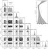 |
Fig. 2 Retrieval results of the fiducial model applied to SP-TW (the spectrum produced in our work), showing the posterior distributions of the molecular mixing ratios. Marginalised posterior distributions (main diagonal) show the parameter estimate median (points) and CCI95 (error bar). The inset plot on the top right shows the median retrieved p-T profile (dashed line) and CCI95 (shaded region). |
4.1 Atmospheric retrieval of SP-TW
In Fig. 2, we show the parameter posterior distributions of the molecular mixing ratios of our fiducial model, as well as the retrieved p-T profile. Figure 3 illustrates the resulting model and uncertainty, as well as the individual opacity contributions based on the finalised model setup. A detailed list of the parameter estimates for all model parameters is given in Table 4.
The main molecules contributing to the transmission spectrum are H2O, CO2, and H2S. H2O shows a broad absorption feature from 2.3 to 3.5 μm, with an inferred mixing ratio of log10(XH2O) ∈ [−1.04, −0.75]. Similarly, CO2 shows a prominent absorption feature centred at 4.4 μm, and a secondary one centred at 2.8 μm. We find log10(XCO2) ∈ [−2.23, −1.86]. In addition to these two constituents, we find a contribution from H2S, with log10(XH2S) ∈ [−2.97, −2.05]. In the spectrum, H2S produces a broad feature from 3.5 to 4.5 μm, and a more narrow feature centred at 2.6 μm. All three of these species are constrained within 0.5dex (for H2O and CO2) and 1dex (for H2S) in the CCI95, indicating that the underlying spectrum provides a significant amount of information to confidently constrain the molecular mixing ratios.
We only find upper limits for the mixing ratios of CO and CH4. This is represented in Fig. 2 by their flat posterior distributions with sharp edges at the estimated upper limits. CO has no significant absorption signature in the wavelength range of SP-TW. Consequently, the corresponding upper limit of the CCI95 (log10(XCO) < -2.74) is a very broad constraint, encompassing most of the prior range. In contrast to this, CH4 has a well-known absorption feature centred at 3.4 μm, within the range of SP-TW. Therefore, the posterior distribution shows a more constraining upper limit of log10(XCH4) < -5.28 in its mixing ratio, given the lack of this feature.
Our fiducial model also includes SO2, C2H2, and HCN. The corresponding parameter estimates are log10(XSO2) ∈ [−10.46, −3.96], log10(XC2H2) ∈ [−9.99, −4.30], and log10(XHCN) ∈ [−11.75, −4.48], respectively. All three of these posterior CCIs are very wide (approximately 5.5 to 7.0 dex), implying that none of these mixing ratios are well constrained beyond upper limits. However, we point out the difference in the shapes of their respective posterior distributions (shown in Fig. 2). Equivalent to CO and CH4, the posterior distribution of HCN represents an upper limit with log10(XHCN) < -4.48, indicated by a distribution that is close to uniform in shape up to this boundary. In contrast to that, the posteriors of SO2 and C2H2 appear to be close to normal distributions. This is reflected by the fact that the median values of log10(XSO2) = 4-.66 and log10(XC2H2) = −4.86 are not centred in the CCI95, but rather skewed towards their upper edge. In these cases, calculating a CCI of width 1σ would provide a wrong sense of confidence in the parameter estimation. In the example of SO2, the equivalent 1σ CCI (expressed in commonly used point estimate and uncertainty values) is  . This would scale the actual lower boundary of the CCI95 to almost 7σ, rather than 2σ, highlighting the importance of properly calculating parameter estimation ranges, rather than scaling apparent σ values.
To contextualise these parameter estimates, we compare the results reported in our work to previously published analyses. We note that the previous works we compare our results to here have all reported retrievals performed with a ‘free’ chemistry approach, enabling a clear comparison of the parameter estimates. Before the launch of JWST, one of the main atmospheric species accessible to transmission spectroscopy performed with HST (the previous state-of-the-art) was H2O. Tsiaras et al. (2018) used two transits of WASP-39 b from HST WFC3 to infer an H2O mixing ratio of log10(XH2O) = −5.94 ± 0.61. In contrast to that, Wakeford et al. (2018) combined HST STIS and WFC3 measurements with Spitzer IRAC and VLT FORS2 data to derive  . Analysing the same dataset, Welbanks et al. (2019) report a prior-dependent value of
  . The H2O mixing ratio reported from our retrievals is in agreement with the latter two, but the range of retrieved abundances from these analyses covers five orders of magnitude, indicating a poor overall agreement on the constraints of the H2O mixing ratio from HST-era observations.
With the advent of JWST, a significantly larger portion of possible atmospheric constituents has become accessible through absorption signatures in the near- and mid-infrared. Constantinou et al. (2023) performed atmospheric retrievals on the cut-off NIRSpec PRISM spectrum of WASP-39 b (JWST Transiting Exoplanet Community Early Release Science Team et al. 2023). From a spectrum derived with Eureka!, they infer a H2O mixing ratio of  . Additionally, they report precise posterior constraints on CO2, SO2, CO, and H2S. Compared to these, the results reported from our retrieval are generally higher by two to three orders of magnitude in the cases of H2O, CO2, and H2S. However, we note that the results reported by Constantinou et al. (2023) also show a variation of approximately 1 dex when considering spectra from different pipelines. The values of SO2 and CO fall within the broad constraints reported from our retrievals. Lueber et al. (2024) studied the information content in the panchromatic transmission spectrum of WASP-39 b. While using the full-range NIRSpec PRISM transmission spectrum presented in Rustamkulov et al. (2023), they find a (cloud-model dependent) value of
  . Similar to Constantinou et al. (2023), they report a much more precise posterior constraint on CO and SO2 than our results suggest, with values of
  and
and  , respectively, which fall within the broad constraints reported from our retrievals. Values for the mixing ratios of CO2 and H2S are smaller by two orders of magnitude compared to our results.
We note that all constraints shown here to contextualise our results were reported as point-estimates with uncertainties equivalent to a 1σ CCI. While we cannot feasibly reproduce the corresponding posterior distributions to derive CCI95 values for a direct comparison, we point out that, especially in cases where the reported uncertainties are asymmetric (such as the H2O mixing ratio from Welbanks et al. 2019), calculating CCI boundaries would be necessary rather than scaling the reported uncertainties. This would potentially result in closer agreement between the here listed results and the parameter estimates from our retrievals.
Lastly, Fig. 2 also illustrates the retrieved p-T profile, represented by the median profile (dashed line) and corresponding CCI95 envelope (shaded area). The temperature values in the middle of the atmospheric pressure domain (given as Tp1 and Tp2 in Table 4) are constrained within approximately 500 K and indicate a close-to isothermal behaviour in this region of the atmosphere. In contrast to that, the temperature nodes at the bottom and top of the atmosphere (Tp0 and Tp3 in Table 4) are less well constrained. The temperature at the top-most pressure node (p = 10−9 bar) has a CCI width of 1500 K (half the prior space). The atmosphere is fully transparent at this pressure level, indicating that there is little information to constrain the temperature of this region. While the thermospheres of hot Jupiters are expected to be heated by the absorption of XUV radiation (Fortney et al. 2021), the retrieval model setup indicates that this temperature increase could be a model degeneracy with the simplified vertical chemical structure (Schleich et al. 2024). The temperature at the bottom-most pressure node (p0 = 10 bar) is even less constrained with a CCI width if 2400 K, encompassing almost the entire prior range. The top of the flat-opacity cloud deck is constrained to log10(pcloud[bar]) < -3.29. Consequently, the lower region of the atmosphere is not accessible in the transmission spectrum of WASP-39 b, resulting in an unconstrained posterior for this temperature node.
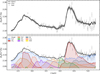 |
Fig. 3 Transmission spectrum with model fit solution from model tuning process. Both panels show wavelength (in μm) on the x-axis against transit depth (in %) on the y-axis, as well as the data points and error bars (grey) from the spectrum produced in this work (SP-TW). (Top) Median model solution (solid black line) and corresponding 95% CCI (shaded area). (Bottom) Contributions of individual molecular opacity sources (colour-coded by molecule) and the flat-opacity cloud deck (dashed grey line). |
Estimated parameters for atmospheric retrievals performed on the spectra used in this work.
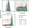 |
Fig. 4 Posterior distributions of select forward model parameters for atmospheric retrievals on scattered instances of SP-TW, showing inferred parameter values (x-axis) against weighted counts (y-axis) in all panels. The parameter posterior distributions are the VMRs of CO2 (top left), CO (top right), and SO2 (bottom right). Marginalised posteriors and CCIs from the initial instance of SP-TW are shown in black, while the results from the scattered instances of SP-TW are colour-coded. |
4.2 Sensitivity to random scatter
As shown in Fig. 2, the posterior distributions of the SO2 and C2H2 mixing ratios have tails towards low abundances. As the parameter inference process in a Bayesian framework is guided by the underlying dataset, this could indicate that the abundances of these molecules are estimated over only a few data points. To test the robustness of the reported parameter estimates to perturbations of the underlying spectrum, we conduct the same homogenised atmospheric retrievals on 10 self-scattered instances of SP-TW. We find that the resulting posterior distributions and derived parameter estimates can be categorised into three types: (1) stable and well constrained, (2) stable and unconstrained, and (3) unstable and skewed. A selection of these is illustrated in Fig. 4. We show a full overview of all marginalised posterior distributions in Fig. C.1. We also list the results from a two-sample K-S test in Table C.1, which compares the marginalised posterior distributions of the scattered instances with the ones from the original instance of SP-TW.
For posterior distributions previously identified as well constrained, we find that the parameter estimates are stable against the perturbations of the spectrum. This is shown in the top left panel of Fig. 4 by the posterior distribution of log10(XCO2). In all cases, the shape of the posterior distribution remains close to being Gaussian, and the CCIs agree with the parameter estimation results retrieved from the baseline instance of SP-TW. This can be explained by the fact that for all stable, well-constrained cases (H2O, CO2, and H2S), the spectral features are mapped onto a broad wavelength range (as can be seen in Fig. 3).
Parameter estimation results identified as upper or lower limits are similarly stable against these perturbations. This is illustrated in the top right panel of Fig. 4 for CO. As it has no significant absorption features in the wavelength range of SP-TW, perturbing the spectrum will have no significant influence on the parameter inference of log10(XCO).
Finally, we find posterior distributions and parameter estimates that are unstable under perturbations of the spectrum. This is shown for SO2 in the bottom left panel of Fig. 4. The mixing ratio parameter estimates of SO2 and C2H2 depend on small regions of the transmission spectrum. Subsequently, scattered instances that influence these regions specifically will produce strong variations in the extent of the associated parameter estimation result. In addition to the tailed posterior distributions described before, in the case of SO2 and C2H2, we find several instances with narrow parameter estimates, mirroring the well constrained mixing ratios of H2O, CO2, and H2S. We also find several instances representing upper limits, with broad ranges for the CCI95 and a centred median. We point out that this behaviour can also, to a lesser extent, be seen in the posterior distributions of CH4. While in its initial instance, the inferred mixing ratio of CH4 is interpreted as an upper limit, we find several instances where the CCI95 resembles the tailed cases we have found for SO2 and C2H2. As CH4 has an absorption feature at 3.4 μm, these instances represent cases where the scattering induces a clearer identification of this feature.
Results from a two-sample K-S test on these distributions indicate that none of the marginalised posteriors share an underlying distribution with the marginalised posteriors from the retrieval performed on the unperturbed SP-TW (Table C.1). However, performing a statistical test on the marginalised posterior distributions neglects information contained in the covariances of these parameters. In reporting atmospheric retrieval results, parameter estimates derived from posterior distributions are the more pertinent conclusions. We find that, even in the unstable cases of SO2, C2H2, and CH4, all CCI95 values agree with the initial results from SP-TW (Fig. C.1). While random perturbations of the input data do not produce disagreement in parameter estimation results, the associated parameter constraints could be overconfidently small. We therefore argue that the assignment of specific VMR values for atmospheric trace species should be interpreted with caution, especially when the credible interval of the parameter posterior is heavily skewed.
4.3 Homogenised atmospheric retrievals on existing transmission spectra
As shown in Fig. 1, the three transmission spectra of WASP-39 b considered in this work show systematic differences. While a random perturbation of SP-TW did not produce disagreement in the resulting atmospheric retrieval results, we now investigate the impact of systematic differences stemming from variations in data reduction assumptions.
As these three spectra were derived from the same underlying raw observation, we assume that they should contain the same information on the nature of the atmosphere of WASP-39 b. Under this assumption, we do not perform additional model tuning on RU-23 and CA-24 (we show a comparison of the values of ln Bm0 derived from retrievals based on each of the three spectra considered in our work in Fig. B.1). Instead, we perform atmospheric retrievals on RU-23 and CA-24 with a homogenised setup from the model tuning on SP-TW. Figure 5 shows a comparison between the parameter posteriors of the molecular mixing ratios and cloud-top pressure for all three retrieval cases, as well as the associated p-T profiles. A comprehensive list of all parameter estimates is given in Table 4.
Generally, all three retrieval cases produce results that agree within the CCI95 values. The mixing ratios of H2O and CO2 are well constrained, with posterior distributions that are close to Gaussian and a parameter estimation range that spans 0.5 to 1 dex. Similarly, the mixing ratios of CO, CH4, and HCN are constrained to upper limits based on the retrieval performed on all three spectra. We note that in the case of RU-23, the upper limit on CH4 is approximately one order of magnitude smaller than in the other two cases. When comparing all three spectra in Fig. 1, RU-23 shows lower transit depths in the region of the methane absorption feature at 3.4 μm, which could explain this reduced upper limit. Additionally, the posterior distribution of CO derived from RU-23 shows a stronger peak towards the upper edge of the parameter estimation range, indicated by the positively shifted median of the posterior distribution.
We find the biggest differences in the molecular mixing ratios previously categorised as unstable, skewed cases (SO2 and C2H2). In the case of C2H2, the tailed posterior from SP-TW is contrasted by two uniform posterior distributions denoting upper limits of log10(XC2H2) < -5.89 and log10(XC2H2) < -5.36 in the case of RU-23 and CA-24, respectively. In the case of SO2, we see the largest variety in posterior behaviour. The skewed posterior distribution from SP-TW is contrasted by an unconstrained mixing ratio in the case of CA-24 (with log10(XSO2) < -4.38), and a much narrower constraint from RU-23 (with log10(XSO2) ∈ [−5.48, −4.57]). For both C2H2 and SO2, all three retrieved parameter estimates are still in agreement in this case, but the behaviour of the associated posterior distributions mirrors the unstable and skewed case identified in the retrievals of the scattered instances of SP-TW (bottom left panel of Fig. 4).
We also find one case of a disagreement in the parameter estimation results, which is the mixing ratio of H2S. For both RU-23 and CA-24, a narrow posterior on its mixing ratio is replaced by a skewed distribution with with log10(XH2S) ∈ [−9.77, −3.15] and with log10(XH2S) ∈ [−9.25, −2.28], respectively. The parameter estimate of H2S from RU-23 does not overlap with the posterior constraints from SP-TW, although the disagreement is smaller than 0.2 dex.
Finally, the retrieved p-T profiles agree between all three cases. The close-to-isothermal structure in the middle of the atmospheric domain is preserved, and all cases struggle to constrain the temperature values at the top and bottom of the atmosphere. We point out that the retrievals of SP-TW and RU-23 indicate a thermal inversion in the upper layers of the atmosphere. The retrieval of CA-24 has a broader posterior of the temperature at the top of the atmosphere, being consistent with both an isothermal behaviour, as well as an increasing temperature profile. The retrieved cloud-top pressure is in close agreement for all three retrievals, which, as a flat-opacity layer, masks regions below the value of pcloud as inaccessible for all three spectra.
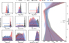 |
Fig. 5 Results of atmospheric retrieval performed on three transmission spectra derived from the same observation. Results achieved with SP-TW (the spectrum produced in our work), as well as with RU-23 and CA-24, are shown in black, red, and blue, respectively. (Left) The grid of smaller panels shows the marginalised posterior distributions of the molecular mixing ratios and cloud-top pressure (Right) Retrieved 4-point pressure temperature profiles, where dashed lines indicate the posterior median, and shaded area the corresponding CCI95. |
4.4 Limitations
The range of reported mixing ratios for the atmospheric constituents of WASP-39 b is very large. An immediate comparison between our results and previous analyses of the NIRSpec PRISM dataset shows higher mixing ratios of the dominant atmospheric trace species from our retrievals (~14% H2O and ~1% CO2). Accounting for previous analyses of HST observations, as well as of observations by the other instruments of JWST, shows instrument- and model-dependent discrepancies as large as five orders of magnitude for these main trace species (e.g. Tsiaras et al. 2018; Wakeford et al. 2018; Lueber et al. 2024). Exoplanet atmospheres are inherently more complex than retrieval models usually account for, reducing a multidimensional problem into a 1D atmospheric slice. In our work, we address the differences in characterisation results stemming from the underlying dataset through a relative result comparison from homogenised atmospheric retrievals. As such, we circumvent the problem of disagreeing results by applying the same model setup to data derived from the same underlying observation. We leave the solution to addressing this tension in results to future work.
We do note that using homogenised atmospheric retrievals on all three spectra overlooks the model-tuning possibility with respect to RU-23 and CA-24. All transmission spectra considered in this work were derived from the same raw data. We therefore make the assumption that the model tuning process is independent of the underlying transmission spectrum. This will not necessarily be the case, as the model-tuning process is guided by the data. As shown in Fig. 1, the spectra show systematic differences, which might propagate into the molecule selection process. While a full comparison to a flexible model-tuning approach is beyond the scope of this work, we note that individualised model setups for SP-TW, RU-23, and CA-24 could produce a smaller range of overlapping molecular constituents. An example of this is the unconstrained nature of the C2H2 posterior distribution in both the case of the RU-23 and CA-24 retrieval.
We also note that our work does not address the importance of individual data reduction steps on the results of atmospheric retrievals. Previous work has reported on the impact of using different data reduction pipelines (e.g. Mugnai et al. 2024; Powell et al. 2024; Davenport et al. 2025). Our work highlights the differences in parameter estimates from spectra independently derived using the same pipeline. Follow-up investigations into the importance of individual steps during data reduction could provide even more insights into the stability of atmospheric retrieval posteriors.
Finally, as the parameter estimation uncertainty represents a subjective choice of the credible interval size, we caution against over-interpreting disagreements on the level of 1σ. As illustrated in Sect. 4.1, skewed posterior distributions will result in much broader directly calculated σ-equivalent CCIs, compared to values scaled from 1σ.
5 Conclusion
Parameter estimation processes in Bayesian inference networks are guided by observational data. In this work, we investigated the impact of data perturbations on the retrieval posteriors of atmospheric parameters from the transmission spectrum of the hot Jupiter WASP-39 b.
We produced a transmission spectrum from a NIRSpec PRISM observation of WASP-39 b, and selected an atmospheric forward model based on this dataset. From a baseline model containing absorption contributions of H2O, CO2, CO, and CH4, we construct a fiducial model with additional contributions from H2S, SO2, C2H2, and HCN. To investigate the reliability of the reported parameter posteriors, we performed homogenised atmospheric retrievals on several additional transmission spectra of WASP-39 b. We performed these retrievals on self-scattered instances of the transmission spectrum produced in our work, which mimics potentially random variations caused by assumptions made during data reduction. We also used two previously published transmission spectra of WASP-39 b, which were derived from the same underlying observation. We find that several forward model parameters (the planetary reference radius, cloud-top pressure, and p-T profile) show no significant variations under the perturbations of the transmission spectrum. The p-T profile is well constrained in the probed region of the atmosphere. The retrieved temperature values at the top and bottom of the atmospheric domain are unconstrained.
In the parameter posteriors of the molecular mixing ratios, we identify three types of behaviour:
Well-constrained posteriors that are close to Gaussian distributions (H2O, CO2, and H2S), resulting in parameter estimates which are stable under the perturbations characterised by the selection of spectra we use.
Posteriors constrained by upper limits (CO and HCN), which result in parameter estimates that are also stable under these perturbations.
Skewed posterior distributions with heavy tails (SO2, C2H2, and CH4), which produce unstable parameter estimates under the cases considered in our work.
When compared to our reference of performing retrievals on the spectrum produced in our work (SP-TW), we find general agreement between the inferred parameter values of atmospheric retrievals performed on different instances of the transmission spectrum of WASP-39 b. However, we emphasise the impact of unstable posterior distributions on the interpretation of these parameter constraints. Heavily skewed parameter posteriors, from which small credible intervals (CIs), such as a 1σ-equivalent, are derived, can provide a misleading sense of accuracy in the inferred values. Directly calculating CIs can reveal these tails clearly and help identify unstable forward model parameters.
Data availability
An online repository with all data products produced and used in this work, as well as supplementary plots, can be found at https://doi.org/10.5281/zenodo.15697940. We also gratefully acknowledge the use of open-source packages for the Python programming language: corner (Foreman-Mackey 2016), matplotlib (Hunter 2007), numpy (Harris et al. 2020), scipy (Virtanen et al. 2020).
Acknowledgements
We would like to thank the anonymous referee for their insightful comments and feedback. S.S. thanks J. Davey for an insightful discussion on error bar asymmetries in atmospheric retrievals, and K. H. Yip for insights on distribution distance metrics. This project was funded by the FGGA Emerging Field Grant 2021. We acknowledge financial support by the University of Vienna and Österreichische Forschungsgemeinschaft (ÖFG). This work is based in part on observations made with the NASA/ESA/CSA James Webb Space Telescope. The data were obtained from the Mikulski Archive for Space Telescopes at the Space Telescope Science Institute, which is operated by the Association of Universities for Research in Astronomy, Inc., under NASA contract NAS 5-03127 for JWST. These observations are associated with program #1366. The authors acknowledge the Transiting Exoplanet Community Early Release Science Program team for developing their observing program with a zero-exclusive-access period. The computational results have been achieved in part using the Austrian Scientific Computing (ASC) infrastructure.
References
- Abel, M., Frommhold, L., Li, X., & Hunt, K. L. C. 2011, J. Phys. Chem. A, 115, 6805 [NASA ADS] [CrossRef] [Google Scholar]
- Abel, M., Frommhold, L., Li, X., & Hunt, K. L. C. 2012, J. Chem. Phys., 136, 044319 [NASA ADS] [CrossRef] [Google Scholar]
- Adam, A. Y., Yachmenev, A., Yurchenko, S. N., & Jensen, P. 2019, J. Phys. Chem. A, 123, 4755 [NASA ADS] [CrossRef] [Google Scholar]
- Ahrer, E.-M., Stevenson, K. B., Mansfield, M., et al. 2023, Nature, 614, 653 [NASA ADS] [CrossRef] [Google Scholar]
- Al-Refaie, A. F., Changeat, Q., Waldmann, I. P., & Tinetti, G. 2021, ApJ, 917, 37 [NASA ADS] [CrossRef] [Google Scholar]
- Al-Refaie, A. F., Changeat, Q., Venot, O., Waldmann, I. P., & Tinetti, G. 2022, ApJ, 932, 123 [NASA ADS] [CrossRef] [Google Scholar]
- Alderson, L., Wakeford, H. R., Alam, M. K., et al. 2023, Nature, 614, 664 [NASA ADS] [CrossRef] [Google Scholar]
- August, P. C., Bean, J. L., Zhang, M., et al. 2023, ApJ, 953, L24 [CrossRef] [Google Scholar]
- Azzam, A. A. A., Tennyson, J., Yurchenko, S. N., & Naumenko, O. V. 2016, MNRAS, 460, 4063 [NASA ADS] [CrossRef] [Google Scholar]
- Barber, R. J., Strange, J. K., Hill, C., et al. 2014, MNRAS, 437, 1828 [CrossRef] [Google Scholar]
- Barstow, J. K., & Heng, K. 2020, Space Sci. Rev., 216, 82 [NASA ADS] [CrossRef] [Google Scholar]
- Barstow, J. K., Changeat, Q., Garland, R., et al. 2020, MNRAS, 493, 4884 [NASA ADS] [CrossRef] [Google Scholar]
- Bell, T. J., Ahrer, E.-M., Brande, J., et al. 2022, JOSS, 7, 4503 [Google Scholar]
- Bell, T. J., Welbanks, L., Schlawin, E., et al. 2023, Nature, 623, 709 [Google Scholar]
- Benneke, B., & Seager, S. 2013, ApJ, 778, 153 [Google Scholar]
- Birkmann, S. M., Ferruit, P., Giardino, G., et al. 2022, A&A, 661, A83 [NASA ADS] [CrossRef] [EDP Sciences] [Google Scholar]
- Blecic, J., Dobbs-Dixon, I., & Greene, T. 2017, ApJ, 848, 127 [NASA ADS] [CrossRef] [Google Scholar]
- Buchner, J., Georgakakis, A., Nandra, K., et al. 2014, A&A, 564, A125 [NASA ADS] [CrossRef] [EDP Sciences] [Google Scholar]
- Burnham, K. P., & Anderson, D. R. 2004, Sociol. Methods Res., 33, 261 [Google Scholar]
- Bushouse, H., Eisenhamer, J., Dencheva, N., et al. 2024, JWST Calibration Pipeline, Zenodo [Google Scholar]
- Caldas, A., Leconte, J., Selsis, F., et al. 2019, A&A, 623, A161 [NASA ADS] [CrossRef] [EDP Sciences] [Google Scholar]
- Carter, A. L., May, E. M., Espinoza, N., et al. 2024, Nat. Astron., 8, 1008 [Google Scholar]
- Changeat, Q., Edwards, B., Waldmann, I. P., & Tinetti, G. 2019, ApJ, 886, 39 [NASA ADS] [CrossRef] [Google Scholar]
- Changeat, Q., Al-Refaie, A. F., Edwards, B., Waldmann, I. P., & Tinetti, G. 2021, ApJ, 913, 73 [NASA ADS] [CrossRef] [Google Scholar]
- Chubb, K. L., Tennyson, J., & Yurchenko, S. N. 2020, MNRAS, 493, 1531 [NASA ADS] [CrossRef] [Google Scholar]
- Chubb, K. L., Rocchetto, M., Yurchenko, S. N., et al. 2021, A&A, 646, A21 [NASA ADS] [CrossRef] [EDP Sciences] [Google Scholar]
- Claret, A. 2000, A&A, 363, 1081 [NASA ADS] [Google Scholar]
- Coles, P. A., Yurchenko, S. N., & Tennyson, J. 2019, MNRAS, 490, 4638 [CrossRef] [Google Scholar]
- Constantinou, S., Madhusudhan, N., & Gandhi, S. 2023, ApJ, 943, L10 [NASA ADS] [CrossRef] [Google Scholar]
- Cox, A. N. 2015, Allen’s Astrophyiscal Quantities (Berlin: Springer) [Google Scholar]
- Davenport, B., Kempton, E. M.-R., Nixon, M. C., et al. 2025, ApJ, 984, L44 [Google Scholar]
- Davey, J. J., Yip, K. H., Al-Refaie, A. F., & Waldmann, I. P. 2025, MNRAS, 536, 2618 [Google Scholar]
- Dyrek, A., Min, M., Decin, L., et al. 2024, Nature, 625, 51 [Google Scholar]
- Edwards, B., & Changeat, Q. 2024, ApJ, 962, L30 [NASA ADS] [CrossRef] [Google Scholar]
- Edwards, B., Changeat, Q., Mori, M., et al. 2021, AJ, 161, 44 [Google Scholar]
- Edwards, B., Tsiaras, A., Changeat, Q., & Yip, K. H. 2024, RAS Techn. Instrum., 3, 415 [Google Scholar]
- Espinoza, N., & Jones, K. 2021, AJ, 162, 165 [NASA ADS] [CrossRef] [Google Scholar]
- Faedi, F., Barros, S. C. C., Anderson, D. R., et al. 2011, A&A, 531, A40 [NASA ADS] [CrossRef] [EDP Sciences] [Google Scholar]
- Feinstein, A. D., Radica, M., Welbanks, L., et al. 2023, Nature, 614, 670 [NASA ADS] [CrossRef] [Google Scholar]
- Feroz, F., Hobson, M. P., & Bridges, M. 2009, MNRAS, 398, 1601 [NASA ADS] [CrossRef] [Google Scholar]
- Fletcher, L. N., Gustafsson, M., & Orton, G. S. 2018, ApJS, 235, 24 [NASA ADS] [CrossRef] [Google Scholar]
- Foreman-Mackey, D. 2016, JOSS, 1, 24 [NASA ADS] [CrossRef] [Google Scholar]
- Foreman-Mackey, D., Hogg, D. W., Lang, D., & Goodman, J. 2013, PASP, 125, 306 [Google Scholar]
- Fortney, J. J., Dawson, R. I., & Komacek, T. D. 2021, JGR Planets, 126, e2020JE006629 [Google Scholar]
- Fu, G., Stevenson, K. B., Sing, D. K., et al. 2025, ApJ, 986, 1 [Google Scholar]
- Gardner, J. P., Mather, J. C., Abbott, R., et al. 2023, PASP, 135, 068001 [NASA ADS] [CrossRef] [Google Scholar]
- Gelman, A., Hwang, J., & Vehtari, A. 2014, Stat. Comput., 24, 997 [Google Scholar]
- Gordon, I. E., Rothman, L. S., Hargreaves, R. J., et al. 2022, JQSRT, 277, 107949 [CrossRef] [Google Scholar]
- Grant, D., & Wakeford, H. R. 2022, Zenodo [Google Scholar]
- Harris, C. R., Millman, K. J., van der Walt, S. J., et al. 2020, Nature, 585, 357 [NASA ADS] [CrossRef] [Google Scholar]
- Horne, K. 1986, PASP, 98, 609 [Google Scholar]
- Hunter, J. D. 2007, Comput. Sci. Eng., 9, 90 [NASA ADS] [CrossRef] [Google Scholar]
- Jakobsen, P., Ferruit, P., de Oliveira, C. A., et al. 2022, A&A, 661, A80 [NASA ADS] [CrossRef] [EDP Sciences] [Google Scholar]
- JWST Transiting Exoplanet Community Early Release Science Team, Ahrer, E.-M., Alderson, L., et al. 2023, Nature, 614, 649 [NASA ADS] [CrossRef] [Google Scholar]
- Kass, R. E., & Raftery, A. E. 1995, J. Am. Stat. Assoc., 90, 773 [Google Scholar]
- Keers, R. E., Shapiro, A. I., Kostogryz, N. M., et al. 2024, ApJ, 977, L7 [Google Scholar]
- Kempton, E. M.-R., Zhang, M., Bean, J. L., et al. 2023, Nature, 620, 67 [NASA ADS] [CrossRef] [Google Scholar]
- Kreidberg, L. 2015, PASP, 127, 1161 [Google Scholar]
- Li, G., Gordon, I. E., Rothman, L. S., et al. 2015, ApJS, 216, 15 [NASA ADS] [CrossRef] [Google Scholar]
- Lueber, A., Novais, A., Fisher, C., & Heng, K. 2024, A&A, 687, A110 [NASA ADS] [CrossRef] [EDP Sciences] [Google Scholar]
- Lustig-Yaeger, J., Fu, G., May, E. M., et al. 2023, Nat. Astron., 1 [Google Scholar]
- MacDonald, R. J., Goyal, J. M., & Lewis, N. K. 2020, ApJ, 893, L43 [NASA ADS] [CrossRef] [Google Scholar]
- Madhusudhan, N. 2019, ARA&A, 57, 617 [NASA ADS] [CrossRef] [Google Scholar]
- Madhusudhan, N., Sarkar, S., Constantinou, S., et al. 2023, ApJ, 956, L13 [NASA ADS] [CrossRef] [Google Scholar]
- Magic, Z., Chiavassa, A., Collet, R., & Asplund, M. 2015, A&A, 573, A90 [NASA ADS] [CrossRef] [EDP Sciences] [Google Scholar]
- Mancini, L., Esposito, M., Covino, E., et al. 2018, A&A, 613, A41 [NASA ADS] [CrossRef] [EDP Sciences] [Google Scholar]
- Mant, B. P., Yachmenev, A., Tennyson, J., & Yurchenko, S. N. 2018, MNRAS, 478, 3220 [NASA ADS] [CrossRef] [Google Scholar]
- Mollière, P., Molyarova, T., Bitsch, B., et al. 2022, ApJ, 934, 74 [CrossRef] [Google Scholar]
- Moran, S. E., Stevenson, K. B., Sing, D. K., et al. 2023, ApJ, 948, L11 [NASA ADS] [CrossRef] [Google Scholar]
- Morello, G., Tsiaras, A., Howarth, I. D., & Homeier, D. 2017, AJ, 154, 111 [NASA ADS] [CrossRef] [Google Scholar]
- Morello, G., Dyrek, A., & Changeat, Q. 2022, MNRAS, 517, 2151 [NASA ADS] [CrossRef] [Google Scholar]
- Mugnai, L. V., Swain, M. R., Estrela, R., & Roudier, G. M. 2024, MNRAS, 531, 35 [Google Scholar]
- Murphy, M. M., Beatty, T. G., Welbanks, L., & Fu, G. 2025, AJ, 169, 286 [Google Scholar]
- Niraula, P., de Wit, J., Gordon, I. E., et al. 2022, Nat. Astron., 6, 1287 [Google Scholar]
- Niraula, P., de Wit, J., Gordon, I. E., Hargreaves, R. J., & Sousa-Silva, C. 2023, ApJ, 950, L17 [NASA ADS] [CrossRef] [Google Scholar]
- Nixon, M. C., Welbanks, L., McGill, P., & Kempton, E. M.-R. 2024, ApJ, 966, 156 [Google Scholar]
- Pluriel, W., Leconte, J., Parmentier, V., et al. 2022, A&A, 658, A42 [NASA ADS] [CrossRef] [EDP Sciences] [Google Scholar]
- Polyansky, O. L., Kyuberis, A. A., Zobov, N. F., et al. 2018, MNRAS, 480, 2597 [NASA ADS] [CrossRef] [Google Scholar]
- Powell, D., Feinstein, A. D., Lee, E. K. H., et al. 2024, Nature, 626, 979 [NASA ADS] [CrossRef] [Google Scholar]
- Rackham, B. V., Apai, D., & Giampapa, M. S. 2018, ApJ, 853, 122 [Google Scholar]
- Rothman, L. S., Gordon, I. E., Barber, R. J., et al. 2010, JQSRT, 111, 2139 [NASA ADS] [CrossRef] [Google Scholar]
- Rustamkulov, Z., Sing, D. K., Mukherjee, S., et al. 2023, Nature, 614, 659 [NASA ADS] [CrossRef] [Google Scholar]
- Saba, A., Tsiaras, A., Morvan, M., et al. 2022, AJ, 164, 2 [NASA ADS] [CrossRef] [Google Scholar]
- Sarkar, S., & Madhusudhan, N. 2021, MNRAS, 508, 433 [Google Scholar]
- Sarkar, S., Madhusudhan, N., Constantinou, S., & Holmberg, M. 2024, MNRAS, 531, 2731 [Google Scholar]
- Schleich, S., Boro Saikia, S., Changeat, Q., et al. 2024, A&A, 690, A336 [NASA ADS] [CrossRef] [EDP Sciences] [Google Scholar]
- Schmidt, S. P., MacDonald, R. J., Tsai, S.-M., et al. 2025, arXiv eprints [arXiv:2501.18477] [Google Scholar]
- Tennyson, J., Yurchenko, S. N., Al-Refaie, A. F., et al. 2020, JQSRT, 255, 107228 [NASA ADS] [CrossRef] [Google Scholar]
- Tsai, S.-M., Lee, E. K. H., Powell, D., et al. 2023, Nature, 617, 483 [CrossRef] [Google Scholar]
- Tsiaras, A., Waldmann, I. P., Zingales, T., et al. 2018, AJ, 155, 156 [NASA ADS] [CrossRef] [Google Scholar]
- Underwood, D. S., Tennyson, J., Yurchenko, S. N., et al. 2016, MNRAS, 459, 3890 [NASA ADS] [CrossRef] [Google Scholar]
- Vehtari, A., Gelman, A., & Gabry, J. 2017, Stat. Comput., 27, 1413 [Google Scholar]
- Virtanen, P., Gommers, R., Oliphant, T. E., et al. 2020, Nat. Methods, 17, 261 [Google Scholar]
- Voyer, M., Changeat, Q., Lagage, P.-O., et al. 2025, ApJ, 982, L38 [Google Scholar]
- Wakeford, H. R., Sing, D. K., Deming, D., et al. 2018, AJ, 155, 29 [Google Scholar]
- Waldmann, I. P., Tinetti, G., Rocchetto, M., et al. 2015, ApJ, 802, 107 [CrossRef] [Google Scholar]
- Welbanks, L., Madhusudhan, N., Allard, N. F., et al. 2019, ApJ, 887, L20 [NASA ADS] [CrossRef] [Google Scholar]
- Welbanks, L., McGill, P., Line, M., & Madhusudhan, N. 2023, AJ, 165, 112 [NASA ADS] [CrossRef] [Google Scholar]
- Welbanks, L., Nixon, M. C., McGill, P., et al. 2025, arXiv eprints [arXiv:2504.21788] [Google Scholar]
- Yurchenko, S. N., Amundsen, D. S., Tennyson, J., & Waldmann, I. P. 2017, A&A, 605, A95 [NASA ADS] [CrossRef] [EDP Sciences] [Google Scholar]
- Yurchenko, S. N., Mellor, T. M., Freedman, R. S., & Tennyson, J. 2020, MNRAS, 496, 5282 [NASA ADS] [CrossRef] [Google Scholar]
We note that multinest reports the maximised log-likelihood values as part of the sampling run summary statistics in [root]summary.txt (Feroz et al. 2009; Buchner et al. 2014).
Appendix A Opacity sources
References for opacity data used in this work.
Appendix B Model tuning process and metrics
The baseline for our atmospheric forward model contains opacity contributions from CIA of H2-H2 and H2-He pairs, Rayleigh scattering of all molecules, a flat-opacity cloud deck, and molecular absorption from H2O, CO2, CO, and CH4. We assign the index 0 to the baseline model, M0. This model is extended through an investigation into model preference under variations of the considered molecular species.
We evaluate the preference of individual models using multiple metrics. Firstly, we consider the Bayes factor, Bm0, between forward models including new molecules, and the baseline model,
 (B.1)
(B.1)
In this equation, E0 and Em represent the Bayesian evidence of the baseline model and the extended model, respectively. We evaluate the natural logarithm of the Bayes factor, ln Bm0, based on the formalism suggested in Kass & Raftery (1995), which compares the posterior odds of two models under the assumption of equal prior odds of the models. The threshold values associated with this are given in Table 3. If an extended forward model shows ln Bm0 > 3 (corresponding to a posterior odds ratio of more than 20:1), we consider it as significant in our selection process and therefore include it in our finalised model setup.
Secondly, we compare the corrected Akaike Information Criterion (cAIC, henceforth referred to as Ψ) values for all models,
 (B.2)
(B.2)
where n is the sample size (number of transmission spectrum data points in our case), K is the number of free parameters (between 9 and 14 for the models we consider), and L̂ is the maximised log-likelihood3. Ψ provides a second-order correction to the standard AIC for small sample sizes (n < 40K, Burnham & Anderson 2004). Like the Bayes factor, the Ψ is a relative metric, but uses a point-estimate (the maximised likelihood) rather than the marginalised likelihood value of each model. In our model ensemble, we evaluate ∆m = Ψmin - Ψi, where Ψmin is the minium cAIC value within the ensemble, and Ψm the cAIC value for the model Mm. Following the prescription of Burnham & Anderson (2004), we judge that models with values of ∆m < 2 have considerable support compared to the model with Ψmin (translating into a likelihood ratio of approximately 1:3).
Lastly, we calculate the reduced χ-square metric,  , connected to each model. As with Ψ,
  represents a model performance metric judged on a point-estimate as a result of the inference process. In our case, we calculate
  for the median model,
 (B.3)
(B.3)
where (Oi, M̄i,  ) represent the measurement, median model value, and variance associated with data point i, n represents the sample size, and ν = n - K the degrees of freedom of a model with K free parameters. Compared to the other two metrics,
  is an absolute metric measuring the weighted sum of square deviations normalised to the number of degrees of freedom for each model. A summary of the individual model tuning metric values used in our work is provided in Table B.1. In total, we run 23 retrievals during the model tuning.
We point out that a bottom-up model parameter space selection stands in contrast to the top-down model tuning process described in Benneke & Seager (2013). Adding contributions to a small baseline model can exacerbate the value of the Bayes factor and lead to the spurious identification of molecules (Welbanks et al. 2025). Our model tuning process starts from a constrained set of molecules based on prior analyses of WASP-39 b (e.g. Tsiaras et al. 2018, Wakeford et al. 2018, JTERS23). We then evaluate necessary changes to the small baseline model. This model extension process does indeed lead to large changes in the Bayes factor (Table B.1). However, we supplement our initial selection by an analysis of the model performance containing all iterations of the molecules selected in the first step. With this, we confirm that a step-by-step extended model is still preferred over the initial baseline to a sufficiently large degree. Additionally, the Bayes factor is also a purely relative metric. The values of ln Bm0 for models 18, 19, 20, and 21 can be compared with model 22 to look at this selection from a top-down view.
The tuning process we perform in our work is also anchored to the dataset on which it is performed. In Fig. B.1, we show the values of ln Bm0 for model cases run on RU-23 and CA-24. We find that, while the relative behaviour of all three Bayes factor cases shows similar increases for the same models, the absolute values of ln Bm0 are significantly smaller for the retrievals performed on CA-24. The overlapping favoured model setup cases based on each of the input spectra share the inclusion of H2S and SO2. Only model comparisons based on SP-TW and RU-23 additionally favour the inclusion of C2H2 and HCN. However, as all three spectra considered in our work are based on the same underlying observation, we assume that they contain the same information about the nature of the atmosphere of WASP-39 b. Therefore, we use the model setup selected from the model tuning performed on SP-TW (model M22) homogeneously in the comparison with retrievals performed on RU-23 and CA-24. A comprehensive list of all values for the evidence of each model, ln E, can be found in the associated online repository.
Model evaluation metrics for the model tuning process based on the SP-TW dataset.
 |
Fig. B.1 Values of the Bayes factor, ln Bm0, for all model setups considered in this work based on the dataset SP-TW (black), RU-23 (red), and CA-24 (blue). All Bayes factors are computed in reference to the baseline model (M0, see also Table B.1). Values of ln Bm0 are cut off for readability, and dotted lines are inserted as visual guides. The grey areas marked in the figure denote, in decreasing opacity, the Bayes factor threshold values given in Table 3. |
Appendix C Comparison of marginalised posteriors from scattered instances of SP-TW
p-value of the K-S statistic for all marginalised posterior distributions from retrievals of scattered instances of SP-TW.
Appendix D Data reduction
To perform end-to-end data reduction, we use the open-source data reduction pipeline Eureka!4 (Bell et al. 2022). Eureka! acts as both a wrapper for the official jwst pipeline (Bushouse et al. 2024), as well as a framework to perform light-curve fitting. It has been used to successfully perform data reduction and spectra extraction on several JWST observations, including the observations conducted during the ERS programme (e.g. Ahrer et al. 2023; Alderson et al. 2023; Feinstein et al. 2023; Rustamkulov et al. 2023), and multiple other exoplanets (e.g. August et al. 2023; Bell et al. 2023; Kempton et al. 2023; Lustig-Yaeger et al. 2023; Moran et al. 2023; Dyrek et al. 2024). Eureka! is also highly modular, supporting the fine-tuning of data reduction steps to ensure optimal precision in the reduced data products.
Stage 1 of Eureka! acts mostly as a wrapper for steps from the official jwst pipeline, which performs ramp-to-slope fitting. Unless otherwise stated, we use the standard steps recommended for this stage, with the version jwst=1.8.2. We deviate from it by using a 10 σ threshold for the jump_rejection step, instead of the more constraining default threshold of 4 σ. As pointed by JWST Transiting Exoplanet Community Early Release Science Team et al. (2023) (referred to as JTERS23 from here onwards) and Rustamkulov et al. (2023), a threshold this small, combined with the small number of groups for this observation, leads to excessive fractions of detector pixels being flagged as outliers. We therefore choose the larger threshold of 10 σ. Additionally, we perform the group-level background subtraction (GLBS) step introduced in Eureka! v0.7, to account for 1/f-noise introduced during the detector read-out (JTERS23). We mask several pixel coordinates by hand that have, in this step and at the time of data reduction, not yet been flagged as bad pixels5. The background region for this step is defined as being outside of y ∈ [5;22]. For the background, we fit a second-order polynomial, with an outlier rejection threshold of 5 σ. We skip the refpix step, as there are no reference pixels in this sub-array of the detector (Birkmann et al. 2022), as well as the gain_scale step, as the relative flux measurements of interest here do not necessitate flux calibration.
Similar to stage 1, stage 2 of Eureka! is primarily a wrapper for the underlying jwst pipeline, which performs additional calibration and unit conversion steps. Notably, we skip the flat_field step, which at the time of our data reduction did not properly work due to incomplete reference files (e.g. Alderson et al. 2023; Sarkar et al. 2024) We also skip the photom (count-rate to flux-density conversion) and extract_1d steps (1D signal extraction), which are not necessary for our purposes.
In stage 3, we constrain the spectral data in the dispersion direction within the range x ∈ [160; 512]. We do this to exclude the saturated lower end of the spectrum. Saturation in the wavelength region was intentionally achieved to increase the signal-to-noise ratio (S/N) for longer wavelengths (JTERS23). We define the saturation threshold conservatively as 60% of the full-well capacity, to avoid potentially strong influences of the detector non-linearity. This is illustrated in Fig. D.1, which shows the mean count-rate after the first and fifth group the observation for detector row 16, which receives the majority of the signal. As visible in this figure, the median signal over all integrations indicates that the columns below y = 160 are above this threshold, which is where we set the lower limit (we note the exception of column 162, which oscillates around our limit and was included in our accepted range for consistency). We perform a double-iteration outlier-rejection step along the time axis with a threshold of 5 σ, and follow the optimal spectral extraction routine included in Eureka!. For this, we use an aperture with a half-width of 6 pixels, centred at row 16, and a background halfwidth of 9 pixels. We find that the best combination is in an effort to keep the spectral aperture half-width as large as possible (Horne 1986), while maximising the overall precision of the spectrum. We construct the spatial profile through the median frame, and perform outlier rejection with thresholds of 10 σ during the construction of the spatial profile, and a 60 σ during the optimal spectral extraction.
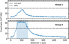 |
Fig. D.1 Median signal for row 16, showing dispersion-direction pixel position on the x-axis, and received signal in DN on the y-axis, for the first (top panel) and fifth (bottom panel) group. The solid black line denotes the full-well value, while the dashed black line marks the 60 % saturation threshold. The blue shaded area indicates the range in dispersion direction that falls above the 60 % saturation threshold. |
Appendix D.1 Extraction of spectroscopic LCs
In stage 4, we restrict the data to wavelengths below 5.3 μm, as the throughput becomes negligible beyond this wavelength regime (Jakobsen et al. 2022). We perform a final round of outlier-rejection in the temporal direction in this stage, using a rolling median from a box-car filter with a width of 100 data points and a rejection threshold of 5 σ, using a maximum of 10 iterations. To identify outliers in the expected precision of the spectroscopic light-curves, we compare the median absolute deviation (MAD) value for each individual light-curve extracted by Eureka! to simulations performed with the JWST Exoplanet Simulator (JexoSim, Sarkar & Madhusudhan 2021). We perform a noise-budget simulation including all noise-sources considered in JexoSim and 10 realisations. We use a simulation setup according to the actual observational parameters, including NIRSpec PRISM instrument setup with five groups per integration and a fixed-bin size of one pixel. System parameters are queried within JexoSim. We then compare the calculated spectroscopic precision for our data reduction with the noise-budget from JexoSim, and flag individual detector-column positions exceeding a threshold of 1.75 times the photon-noise as deviations. These detector-level channels are excluded from further analysis. We show this in Fig. D.2. The integrated whitelight curve is constructed by excluding these flagged detector columns, and performing an additional time-series outlier rejection, using a rolling median with an outlier rejection threshold of 3 σ.
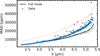 |
Fig. D.2 Spectroscopic light-curve precision, showing wavelength (in μm) on the x-axis, and the median-absolute deviation (MAD, in ppm) on the y-axis. The MAD-values from our data reduction (blue points) are compared to the photon-noise contribution (grey solid line) from a JexoSim simulation. The black solid line shows the corresponding full noise budget, and the grey dashed line represents twice the photon-noise contribution. Individual channels deviating by a factor of 1.75 from the photon-noise contribution (red crosses) are not considered in further analysis. |
To calculate the limb-darkening coefficients corresponding to each spectroscopic, as well as the white-light curve, we use the ExoTiC-LD Python package (Grant & Wakeford 2022) incorporated in Eureka!. We use the stellar parameters given in Table 1, and the Stagger grid of stellar models (Magic et al. 2015).
Appendix D.2 Light-curve fitting
We use a combined astrophysical and systematics model to fit both the pixel-resolution spectroscopic light-curves and the integrated white light-curve resulting from stage 4 of Eureka!. The Python package batman (Kreidberg 2015) is used within Eureka! to calculate transit light-curves, based on a set of astrophysical parameters for the star-planet system through the fraction of blocked stellar flux by the transiting planet. The area of the stellar disk obscured by the transiting planet is determined by the planet radius in units of the host star radius (Rp/R*). The amount of missing flux depends on the projected location of the planet on the stellar disk, and is determined through the time of inferior conjunction (t0), the orbital period (P), the semi-major axis in units of the host star radius (a/R*), as well as the orbital eccentricity (e) and longitude of periastron (w).
An additional influencing factor in the astrophysical transit model is the limb-darkening description. Stellar limb-darkening characterises the intensity gradient of the sky-projected stellar disk. In the case of our fitting routine, we use pre-calculated limb-darkening coefficients from the ExoTiC-LD framework (Grant & Wakeford 2022) corresponding to a 4-parameter non-linear limb-darkening law (Claret 2000). We choose the 4-parameter limb-darkening prescription over the commonly employed quadratic limb-darkening law, which has been shown to introduce biases in the retrieved transit depth (e.g. Morello et al. 2017; Keers et al. 2024). Limb-darkening parameters are calculated for the integrated white-light curve, as well as for the individual spectroscopic light-curves based on the stellar parameters listed in Table 1.
Light-curve fitting parameters
As a model for instrument-dependent systematics, we fit a quadratic global trend with three polynomial coefficients (c0, c1, c2) in time to the median-normalised spectroscopic and integrated white-light curves to produce a combined model. We fit for a total of seven free parameters in the case of the integrated white-light curve. For the spectroscopic light-curves, we fit four free parameters, assuming that the inclination, i, time of inferior conjunction, t0, and scaled semi-major axis, a/R*, are wavelength-independent. These parameters, as well as their associated priors, and the fixed parameters of the astrophysical model are given in Table D.1.
To fit the combined model to each light-curve, we use the Markov chain Monte Carlo (MCMC) sampling algorithm emcee (Foreman-Mackey et al. 2013). In all cases, we run the MCMC chain with 5000 steps using a burn-in phase of 500 steps and 20 walkers. We show the mean auto-correlation time for each spectroscopic channel in Fig. D.3, and find a mean autocorrelation time of approximately 60 steps for the white-light curve fit, which we judge as sufficient for convergence of our MCMC chains (Foreman-Mackey et al. 2013). A summary of the light-curve fitting is shown in Fig. D.4, comparing the 2D, pixelresolution light-curve data to the model fit results and associated fit residuals. Individual columns of increased noise can be seen in the figure, which are flagged as excessively noisy and excluded from the final transmission spectrum.
Appendix D.3 Transmission spectrum binning
To produce the finalised transmission spectrum, we bin the pixel-resolution transit depth values from our spectroscopic light-curve fits using a weighted arithmetic mean (WAM) with a fixed bin size of three,
 (D.1)
(D.1)
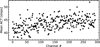 |
Fig. D.3 Convergence of the MCMC chains for each spectroscopic light-curve fit, showing the channel number on the x-axis, and mean auto-correlation time (in number of steps) on the y-axis. We point out that the associated mean autocorrelation time for the white light-curve fit is 60 steps. |
where δ̄ represents the binned transit depth value, which is derived from pixel-resolution transit depth values, δi. The corresponding weights, wi, are defined through the inverse of the associated variance,  . We note that the light-curve fitting determines the transit depth value (as all other parameters in the transit model) through Bayesian inference using MCMC sampling. The reported error bars on δi are defined as mediancentred credible intervals, which are not necessarily symmetric. To calculate the weights, we therefore determine the arithmetic mean of the positive and negative error bars for each transit depth point.
A constant bin size of three pixels accounts for the typically assumed resolution element size of 2.2 pixels for NIRSpec (Jakobsen et al. 2022). We show the finalised transmission spectrum in Fig. D.5, together with the underlying values on a pixel-resolution basis, where flagged pixel-columns (see also Fig. D.2) are marked as red data points, and excluded from the binning process.
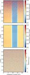 |
Fig. D.4 Data reduction results from Eureka!, showing integration number (equivalent to time) on the x-axis, and wavelength (in μm) on the y-axis. Top: Dynamic light-curve as resulting from stage 4 of Eureka!, with the colour-bar indicating mean-normalised signal. Middle: Combined systematic and astrophysical light-curve fits from stage 5 of Eureka!, with the colour-map representing the same parameters as in the left panel. Bottom: Fit residuals, normalised to the measurement-associated uncertainty. |
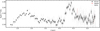 |
Fig. D.5 Transmission spectrum of WASP-39 b produced in this work, showing wavelength (in μm) on the x-axis against transit depth (in %) on the y-axis. Grey data points represent the transit depth values extracted at the pixel-resolution level. Black data points show the finalised transmission spectrum, binned in 3-pixel intervals. Data points marked in red are excluded from this based on Fig. D.2. |
Appendix D.4 Comparison with existing reductions
Table D.2 lists the differences between the data reduction steps applied in this work to derive SP-TW, the Eureka!-ExoTEP data reduction presented in Rustamkulov et al. (2023) to derive RU-23, and the FIREFLy-based data reduction presented in Carter & May et al. (2024) to derive CA-24. Steps not listed are performed with equal assumptions in all three cases.
Main data reduction differences between SP-TW, RU-23, and CA-24.
All Tables
Estimated parameters for atmospheric retrievals performed on the spectra used in this work.
Model evaluation metrics for the model tuning process based on the SP-TW dataset.
p-value of the K-S statistic for all marginalised posterior distributions from retrievals of scattered instances of SP-TW.
All Figures
|
Fig. 1 Comparison of transmission spectra used in this work. Data associated with the spectrum produced in this work (SP-TW) are shown in black, while data associated with Rustamkulov et al. (2023) (RU-23) and Carter & May et al. (2024) (CA-24) are shown in red and blue, respectively. (a) Transmission spectra, showing wavelength (in μm) on the x-axis and transit depth (in %) on the y-axis. (b) Residual distribution of RU-23 and CA-24, normalised to the transit depth uncertainty of SP-TW. For display purposes, the residuals are binned in steps of 0.5 σsp-TW. (c) Empirical cumulative distribution functions (eCDF) for the residuals of RU-23 and CA-24. The values of a one-sample K-S test for a standard normal distribution are given in the legend of the figure. In (b) and (c), the black dashed line represents the PDF and CDF of N(0,1), respectively. |
| In the text | |
|
Fig. 2 Retrieval results of the fiducial model applied to SP-TW (the spectrum produced in our work), showing the posterior distributions of the molecular mixing ratios. Marginalised posterior distributions (main diagonal) show the parameter estimate median (points) and CCI95 (error bar). The inset plot on the top right shows the median retrieved p-T profile (dashed line) and CCI95 (shaded region). |
| In the text | |
|
Fig. 3 Transmission spectrum with model fit solution from model tuning process. Both panels show wavelength (in μm) on the x-axis against transit depth (in %) on the y-axis, as well as the data points and error bars (grey) from the spectrum produced in this work (SP-TW). (Top) Median model solution (solid black line) and corresponding 95% CCI (shaded area). (Bottom) Contributions of individual molecular opacity sources (colour-coded by molecule) and the flat-opacity cloud deck (dashed grey line). |
| In the text | |
|
Fig. 4 Posterior distributions of select forward model parameters for atmospheric retrievals on scattered instances of SP-TW, showing inferred parameter values (x-axis) against weighted counts (y-axis) in all panels. The parameter posterior distributions are the VMRs of CO2 (top left), CO (top right), and SO2 (bottom right). Marginalised posteriors and CCIs from the initial instance of SP-TW are shown in black, while the results from the scattered instances of SP-TW are colour-coded. |
| In the text | |
|
Fig. 5 Results of atmospheric retrieval performed on three transmission spectra derived from the same observation. Results achieved with SP-TW (the spectrum produced in our work), as well as with RU-23 and CA-24, are shown in black, red, and blue, respectively. (Left) The grid of smaller panels shows the marginalised posterior distributions of the molecular mixing ratios and cloud-top pressure (Right) Retrieved 4-point pressure temperature profiles, where dashed lines indicate the posterior median, and shaded area the corresponding CCI95. |
| In the text | |
|
Fig. B.1 Values of the Bayes factor, ln Bm0, for all model setups considered in this work based on the dataset SP-TW (black), RU-23 (red), and CA-24 (blue). All Bayes factors are computed in reference to the baseline model (M0, see also Table B.1). Values of ln Bm0 are cut off for readability, and dotted lines are inserted as visual guides. The grey areas marked in the figure denote, in decreasing opacity, the Bayes factor threshold values given in Table 3. |
| In the text | |
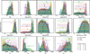 |
Fig. C.1 Same as Fig. 4, but for the marginalised posterior distributions of all parameters. |
| In the text | |
|
Fig. D.1 Median signal for row 16, showing dispersion-direction pixel position on the x-axis, and received signal in DN on the y-axis, for the first (top panel) and fifth (bottom panel) group. The solid black line denotes the full-well value, while the dashed black line marks the 60 % saturation threshold. The blue shaded area indicates the range in dispersion direction that falls above the 60 % saturation threshold. |
| In the text | |
|
Fig. D.2 Spectroscopic light-curve precision, showing wavelength (in μm) on the x-axis, and the median-absolute deviation (MAD, in ppm) on the y-axis. The MAD-values from our data reduction (blue points) are compared to the photon-noise contribution (grey solid line) from a JexoSim simulation. The black solid line shows the corresponding full noise budget, and the grey dashed line represents twice the photon-noise contribution. Individual channels deviating by a factor of 1.75 from the photon-noise contribution (red crosses) are not considered in further analysis. |
| In the text | |
|
Fig. D.3 Convergence of the MCMC chains for each spectroscopic light-curve fit, showing the channel number on the x-axis, and mean auto-correlation time (in number of steps) on the y-axis. We point out that the associated mean autocorrelation time for the white light-curve fit is 60 steps. |
| In the text | |
|
Fig. D.4 Data reduction results from Eureka!, showing integration number (equivalent to time) on the x-axis, and wavelength (in μm) on the y-axis. Top: Dynamic light-curve as resulting from stage 4 of Eureka!, with the colour-bar indicating mean-normalised signal. Middle: Combined systematic and astrophysical light-curve fits from stage 5 of Eureka!, with the colour-map representing the same parameters as in the left panel. Bottom: Fit residuals, normalised to the measurement-associated uncertainty. |
| In the text | |
|
Fig. D.5 Transmission spectrum of WASP-39 b produced in this work, showing wavelength (in μm) on the x-axis against transit depth (in %) on the y-axis. Grey data points represent the transit depth values extracted at the pixel-resolution level. Black data points show the finalised transmission spectrum, binned in 3-pixel intervals. Data points marked in red are excluded from this based on Fig. D.2. |
| In the text | |
Current usage metrics show cumulative count of Article Views (full-text article views including HTML views, PDF and ePub downloads, according to the available data) and Abstracts Views on Vision4Press platform.
Data correspond to usage on the plateform after 2015. The current usage metrics is available 48-96 hours after online publication and is updated daily on week days.
Initial download of the metrics may take a while.