© The Authors 2025

1 Introduction

The stellar mass in low-mass (M_⋆ < 2 M_⊙) stars is set by post-collapse accretion (Lynden-Bell & Pringle 1974; Bertout et al. 1988; Hartmann et al. 1998), with young stellar objects (YSOs) gaining mass by accreting material from the envelope and circumstellar disk. Depending on their spectral energy distributions (SEDs), YSOs can be split into classes from the most embedded protostars (Class 0, I, and Flat Spectrum) to the optically visible pre-main-sequence stars, i.e., Class II and III (see e.g., Greene et al. 1994; André 1995). Although, in the current star formation scenario, the most embedded sources should also be the youngest and the most accreting YSOs, the classification into Classes might not be directly linked to the corresponding evolutionary stage (Enoch et al. 2009).

The accretion luminosity (L_acc) is the parameter that quantifies the energy emitted from the accretion process and play an important role in constraining the evolutionary path of protoplanetary discs. In Class II pre-main sequence stars or Classical T Tauri Stars (CTTSs) the accretion flow from the disk onto the forming star follows the stellar magnetic field lines, as described by the magnetospheric accretion paradigm (Bouvier & Bertout 1986; Hartmann et al. 2016).

The accretion luminosity has been constrained in CTTSs (Valenti et al. 1993; Gullbring et al. 1998; Herczeg & Hillenbrand 2008; Alcalá et al. 2014, 2017; Pittman et al. 2022; Manara et al. 2023, and references therein), where it can be directly measured by modeling the ultraviolet (UV) continuum excess emission (UV excess), generated by the accretion shock, over the stellar photosphere (Calvet & Gullbring 1998; Schneider et al. 2020) and by using empirical correlations between L_acc and U-band excess luminosity (Gullbring et al. 1998; Sicilia-Aguilar et al. 2010). Alternatively, L_acc can be derived using accretion-tracing emission lines (see Fig. 1) and empirical relations between L_acc and the luminosity of the lines (Muzerolle et al. 1998; Herczeg & Hillenbrand 2008; Alcalá et al. 2014, 2017).

Commonly used L_acc − L_line relations are provided in Alcalá et al. (2017). In that work, L_acc was measured adopting the methodologies described in Manara et al. (2013a) namely, by fitting the continuum UV excess. Among other stellar and accretion parameters (see Section 3.1), the procedure yields an estimate of the interstellar extinction, A_V. These A_V values were used to deredden the line fluxes of several accretion tracers (see Fig. 1). The line fluxes were then converted in luminosity, L_line, by adopting a specific distance. This provided a set of L_acc and L_line values for every accretion tracer, from which a relation of the form log(L_acc) = a log(L_line) + b was derived. The sample of CTTSs in Alcalá et al. (2017) is composed by 89 objects in the Lupus star-forming region (hereafter the A17 sample) with spectral types ranging from M8.5 to K0, M_⋆ ~ 0.20–2.15 M_⊙, L_acc ~ 10^−5.4 − 10^−0.25 L_⊙, and L_⋆ ~ 0.003–5.420 L_⊙.

Empirical relations have been used to constrain the accretion luminosity not only on CTTS (e.g., Rugel et al. 2018; Fiorellino et al. 2022a,b; Pouilly et al. 2024), but also on: younger stars classified as protostars (e.g., Fiorellino et al. 2021, 2023; Tychoniec et al. 2024); accreting brown dwarfs (e.g., Whelan et al. 2018; Almendros-Abad et al. 2024); YSOs experiencing episodic accretion, as EXors-like burst (e.g., Singh et al. 2024; Giannini et al. 2024); and even forming-planets (e.g., Haffert et al. 2019; Plunkett et al. 2025; Bowler et al. 2025).

While accurate L_acc measurements must be drawn from data acquired in the widest possible spectral range in the UV, it is important to note that L_acc determinations based on X-shooter data may have the caveat of the spectral range cut at 300 nm (see Fig. 1). The UV Legacy Library of Young Stars as Essential Standards (ULLYSES¹, Roman-Duval et al. 2020) survey is aimed at solving such limitations. ULLYSES utilizes the Hubble Space Telescope (HST) to provide an unprecedented UV spectroscopic library of about 70 CTTSs. The Outflows and Disks around Young Stars: Synergies for the Exploration of Ullyses Spectra (ODYSSEUS², Espaillat et al. 2022) collaboration builds on the ULLYSES survey, utilizing multi-wavelength observations from X-ray to submillimeter in addition to COS and STIS observations, using over 500 HST orbits. The ESO Large Program PENELLOPE³ (Manara et al. 2021) complements the ULLYSES-ODYSSEUS dataset with high-resolution (UVES/ESPRESSO) and flux-calibrated medium-resolution (X-shooter) optical to near-infrared (NIR) spectra from the Very Large Telescope (VLT), contemporaneous to the ULLYSES observations. The ULLYSES-ODYSSEUS-PENELLOPE synergy enables a comprehensive analysis of key accretion and stellar parameters, extinction, and gas kinematics.

The goal of this work is twofold: first, to test whether empirical relation by A17 can be successfully applied to the overall PENELLOPE sample, composed by CTTSs belonging to several star-forming regions; and, second, to compare the empirical relations with those derived from the HST ULLYSES data. We then discuss the applicability of the empirical relations on young accreting objects other than CTTSs.

The paper is structured as follows. In Sect. 2, the samples are described; Section 3 summarizes the methodologies for deriving L_acc for the PENELLOPE and ULLYSES/ODYSSEUS samples, and describe the analysis of the X-shooter data. We also revisit the empirical relations between L_acc and L_line using the ULLYSSES-HST data set, testing the reliability of L_acc estimates obtained through empirical relations by comparing them with values derived from direct UV excess modeling. We then provide an independent method to constrain the A_V of CTTSs using empirical relations, and investigate the possibility for new empirical relations of the Brackett series. Finally, we discuss the results in Sect. 4 and present our conclusions in Sect. 5.

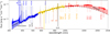Fig. 1 X-shooter spectrum of the CTTS VW Cha. The UVB, VIS and NIR spectra are plotted in blue, yellow, and red, respectively. The UV-excess (blue region), tracing the accretion activity, and the NIR-excess (red region), tracing the presence of an active disk, are highlighted. The black curved dashed line corresponds to a stylized stellar photosphere + continuum veiling. All the accretion tracers for which Alcalá et al. (2017) provided empirical relations are shown in different colors, but not all the lines are labelled in the figure because of limited space. Also Br13, Br11, and Br10 lines are shown. Note: the spectrum starting wavelength was artificially set at ~320 nm for plotting purposes, while the actual UV-cut of X-shooter is at ~300 nm.

2 Data sample

This work analyses the X-shooter spectra from the PENELLOPE project. For a detailed description of the sample and the primary goals of the PENELLOPE observing program, we refer to Manara et al. (2021). We excluded variability monitoring targets, for which dedicated works have already been published (Armeni et al. 2023, 2024; Wendeborn et al. 2024a,b). This results in a sample of 68 YSOs belonging to several star-forming regions: Orion OB1 (8), σOri (3), Chamaeleon I (13), ϵCha (1), ηCha (7), Corona Australis (2), Taurus (8), and Lupus (30), see Table A.1. Among these objects, we have: RECX 5, Lk Ca4, and RXJ0438.6+1546 are Class III YSOs (or weak-line T Tauri stars, WTTSs); AA Tau is a dipper (Bouvier et al. 1999) which lost its regular dipper appearance in 2011 (Bouvier et al. 2013), while its Kepler (K2) light curve from 2017 is dominated by stochastic variability (Cody et al. 2022). The remaining 64 CTTS make up the sample analyzed in this work.

Details on data reduction of the PENELLOPE sample are described in Manara et al. (2021). In a nutshell, the X-shooter data were reduced using a dedicated ESO pipeline (Modigliani et al. 2010), which follows the standard steps including flat, bias, and dark correction, wavelength calibration, spectral rectification, extraction of 1D spectra, and flux calibration using a standard star obtained during the same night. In cases where the signal-to-noise ratio (S/N) of the UVB arm was low (or for resolved binaries) the 1D spectrum was extracted with IRAF⁴. Telluric correction for the VIS and NIR arms was performed using molecfit (Smette et al. 2015; Kausch et al. 2015). Each target was observed first using a set of wide slit (5.0″) in the three arms, leading to a low resolution observation with no slit losses. Then, 1.0″/0.4″/0.4″ wide slits were used for the UVB, VIS, and NIR arms, respectively. The flux calibration was performed by scaling the narrow slits spectra to the wide-slit ones to correct for slit losses. A comparison of the flux calibrated X-Shooter and HST spectra, in the overlapping spectral regions, is shown in Manara et al. (2021). This comparison shows that the flux calibration of the X-shooter spectra is comparable to that of HST. This is important because the precision on the L_acc − L_line relations relies on the precision on L_line determinations; the latter, in turn, depends on the goodness of the flux calibration. All the reduced spectra are publicly available on Zenodo⁵ and on the ESO Phase 3⁶.

The HST data reduction was completed using a custom pipeline at STScI, which was created by the ULLYSES team (Roman-Duval et al. 2025). Details on the data reduction are described in Roman-Duval et al. (2020); Espaillat et al. (2022). We refer to Pittman et al. (2025) for a detail description of the HST sample analysed in this work. For technical reasons, the VLT/X-shooter and HST samples slightly differ in number, resulting in a common sample of 61 sources (see Table 1).

Figure 2 shows the comparison between the log L_acc and M_⋆ distributions of the A17 Lupus, PENELLOPE, and ODYSSEUS samples. The L_acc values were calculated as explained in Sect. 3. The A17 Lupus sample is the only one covering the low-accretion regime down to log L_acc = −5.4, while the ODYSSEUS and PENELLOPE samples are skewed toward higher accretion luminosities, with log L_acc > −4 and log L_acc > −4.5 respectively. The M_⋆ histograms are very alike. We note that the PENELLOPE sample has more sources between 0.6 and 1.0 M_⊙, compared to Lupus and ODYSSEUS samples. We highlight that the ODYSSEUS sample analysed here is a subset of the PENELLOPE catalogue.

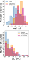Fig. 2 Histograms of accretion luminosity (top) and stellar mass (bottom) for the Lupus sample from (Alcalá et al. 2017, blue), PENELLOPE sample (orange), and ODYSSEUS sample (pink). All histograms are based on the same bin width: 0.5 dex for log Lacc and 0.2 M⊙ for the stellar mass.

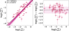Fig. 3 Comparison of Lacc computed using the HST modeling with that from the XS-fit. Left: log $L_{\text{acc\hspace{0.17em}}}^{HST}$ vs. log $L_{\text{acc\hspace{0.17em}}}^{XS}$, the pink line show the best fit, which is linear within the error with its dispersion. Right: differential analysis, the pink region corresponds to the standard deviation of log $L_{\mathrm{a}\mathrm{c}\mathrm{c}}^{HST}$ − log $L_{\mathrm{a}\mathrm{c}\mathrm{c}}^{XS}$, computed as the quadrature sum of the individual errors.

3 Analysis

A major goal of our analysis is to compare the L_acc computed using the hydrogen X-shooter (XS) slab modeling (Manara et al. 2013a) with the multicolumn accretion shock HST model (Pittman et al. 2022), and with those from empirical relations. This process requires:

• a set of L_acc values from both the XS slab modeling (XS-fit) and from the HST multi-columns modeling (HST-fit);

• a derived L_line for every accretion tracer of the PENELLOPE sample;

• empirical relations developed with HST-fit results and comparing to those of the A17 sample;

• L_acc drawn from the L_acc − L_line relations compared with L_acc computed from XS- and HST-fit;

• finally, an investigation of the L_acc validity range of the empirical relations.

Since A_V is a key parameter impacting the L_acc measurement, a further goal is a discussion of the possibility of computing A_V independently, using empirical relations alone. Lastly, since in our sample, several Br series line were detected, we also investigate the possibility of developing new empirical relations in the NIR. The different modelling approaches to determining L_acc and stellar parameters are broadly explained in the PENELLOPE (Manara et al. 2021, Manara et al., in prep.) and ODYSSEUS (Pittman et al. 2022, 2025) papers.

3.1 The X-shooter slab-model

Stellar and accretion parameters were determined using the method originally described by Manara et al. (2013b) and used in the general PENELLOPE papers by Manara et al. (2021). This method has been recently further developed by Claes et al. (2024). Briefly, this approach involves dereddening the observed spectrum across a range of extinction values assuming the reddening law of Cardelli et al. (1989) with R_V = 3.1 and fitting the data with a combination of a photospheric template spectrum and a hydrogen slab model. The slab model, with uniform gas density and temperature, is used to replicate the continuum excess emission observed in the spectrum due to accretion from the disk onto the forming star.

Photospheric templates, from Manara et al. (2013a, 2017), cover spectral types (SpT) from G- to late M-type. A more complete grid of templates is provided in Claes et al. (2024). The integrated flux of the best-fit slab model is used to estimate L_acc, namely, the excess luminosity due to accretion. The SpT gives the T_eff based on the relation by Luhman et al. (2003); Kenyon & Hartmann (1995). The stellar mass is then inferred by interpolating evolutionary tracks from Baraffe et al. (2015) or Siess et al. (2000), depending on the mass.

In this study, we focus extensively on two of the aformentioned parameters: A_V and L_acc, as listed in Table A.1, adopted from Manara et al. (in prep.). The typical error on A_V and L_acc is 0.5 mag and 0.25 dex, respectively, as discussed in A17.

3.2 The HST shock model

Ingleby et al. (2013) introduced an alternative approach to measure the accretion luminosity of CTTSs using the accretion shock model of Calvet & Gullbring (1998). They used multiple accretion columns with varying energy fluxes to account for continuum excesses in the NUV through optical. Recent studies by the ODYSSEUS collaboration (Espaillat et al. 2022; Pittman et al. 2022) applied this method to the first HST observations of the ULLYSES program in Orion OB1b, and it has now been extended to all eight star forming regions in the ULLYSES-PENELLOPE sample by Pittman et al. (2025). Building on the XS-fit parameters as first guess input parameters, Pittman et al. (2022, 2025) derived the extinction and accretion parameters by minimizing the fit to the full 0.2-1.0 μm continuum. We refer to Pittman’s works for a more detailed description of this method.

Pittman et al. (2025) results can be used to compare the XS- and the HST-fit results, as the PENELLOPE X-shooter observations followed-up the ULLYSES-HST observations quasisimultaneously. More in detail, the median time difference between HST and XS data is 1.15 days, while L_acc varies on timescales of days, due to stellar rotation and intrinsic variability. Fig. 3 shows the comparison between the accretion luminosity computed using the HST- and the XS-fit. The left panel shows log $L_{\text{acc\hspace{0.17em}}}^{HST}$ as a function of the log $L_{\text{acc\hspace{0.17em}}}^{XS}$, where log $L_{\text{acc\hspace{0.17em}}}^{HST}$ is measured from the accretion shock model (see Pittman et al. 2025). We performed a linear fit using the hierarchical Bayesian method from Kelly (2007), which accounts for errors on both axes, obtaining $$\log L_{\mathrm{a}\mathrm{c}\mathrm{c}}^{HST}=(0.9\pm 0.1)\log L_{\mathrm{a}\mathrm{c}\mathrm{c}}^{XS}+(0.0\pm 0.2)$$(1)

with a standard deviation σ = 0.2 ± 0.1 and a correlation factor of 0.9. Thus, the best-fit relation between log $L_{\text{acc\hspace{0.17em}}}^{HST}$ and log $L_{\text{acc\hspace{0.17em}}}^{XS}$ is consistent with a one-to-one correlation, indicating that the two estimates are statistically comparable on average. Indeed, for 41% of this sample (26/61) the accretion luminosity computed with the HST- and the XS-fit is in agreement within the error. However, considering individual cases large residuals show-up. The HST-fit method is higher (lower) than the XS-fit method in 24(12) sources, namely, 39%(20%) of the sample. The right panel in Fig. 3 shows the difference of the two accretion luminosity population as a function of the log $L_{\text{acc\hspace{0.17em}}}^{XS}$. The standard deviation of log $L_{\mathrm{a}\mathrm{c}\mathrm{c}}^{HST}$ − log $L_{\mathrm{a}\mathrm{c}\mathrm{c}}^{XS}$ is σ = 0.5. While only nine sources (15%) fall completely outside the 1σ (0.5) region (pink area), eleven additional sources have central values beyond the 1σ range, but still fall within it when uncertainties are taken into account. The observed scatter (σ ~ 0.5 dex) exceeds that expected from formal fitting uncertainties alone (~0.2–0.3 dex), suggesting either underestimated errors or the presence of intrinsic differences between the two methods. We checked how the difference in time between HST and XS observations affected the agreement between the two L_acc measurement (see Appendix B), without finding any significant correlation. Similarly, there is no trend between accretion or stellar parameters and the level of agreement between the two models. Individual discrepancies and a detailed analysis of the large spread in the two distributions will be the focus of a forthcoming paper.

The left panel of Fig. 4 shows the comparison between the A_V values obtained using the HST- and XS-fit. The σ of the distribution is 0.4. The spread is the same for the plot in the right panel, showing the comparison between $A_V^{HST}$ and the extinction computed using empirical relations (see Sect. 3.6).

To investigate whether the scatter in L_acc is driven by differences in A_V, we compared the log L_acc residuals and the A_V residuals. We found a correlation (correlation factor 0.8) between the log L_acc and A_V residuals. This correlation highlights the known degeneracy between L_acc and A_V. We note that a more comprehensive analysis, where the XS spectra are fit fixing $A_V^{HST}$, is something that must be investigated and that we will perform in a forthcoming paper.

Overall, our analysis shows that L_acc derived from HST- and XS-fit are statistically equivalent within the sample. Consequently, we expect empirical relations based on HST data to be statistically equivalent to those from X-shooter.

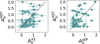Fig. 4 Left: comparison of AV computed using the HST- and XS- modelling. Right: comparison of AV using the HST-fit and the difference method of Sect. 3.6). The dashed line shows the one-to-one relation. The σ in both cases is 0.4.

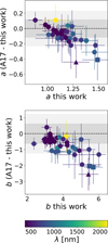Fig. 5 Comparison of the slopes (top) and intercepts (bottom) of the log Lacc − log Llines empirical relations derived in this work with those from Alcalá et al. (2017). The colorbar indicates the corresponding wavelength of each accretion tracer, ranging from UVB (blue) to NIR (yellow). Dark and light gray regions represent agreement within 1σ and 2σ, respectively. Accretion tracers not in agreement within 1σ (2σ) within the error are plotted as squares (triangles).

3.3 Revisiting the L_acc − L_line relations with HST data

Since HST and XS observations were quasi-simultaneous, we used the lines luminosity from the X-shooter PENELLOPE data and the L_acc values drawn from the HST modelling to revisit the L_acc − L_line relationships and compare with the previous A17 X-shooter results. We note, however, that the HST data cover a smaller range in L_acc with respect to the A17 sample.

For the 61 objects observed by both XS and HST, we dereddened the observed PENELLOPE line fluxes (see Appendix C) using extinction values derived from the HST-fit, denoted as $A_V^{HST}$, and we computed their luminosities: L_i = 4πd²F_i, where d is the distance to each source, computed from inverting the parallaxes from Gaia EDR3 (Gaia Collaboration 2021). For each line, i, a best linear fit log $L_{\mathrm{a}\mathrm{c}\mathrm{c}}^i=a_i$ log $L_{\mathrm{a}\mathrm{c}\mathrm{c}}^{HST}+b_i$ was computed as explained in Sect. 3.2. We refer to Appendix D for the details.

Figure 5 shows that the slope and the intercept obtained using the PENELLOPE sample and the HST-fit are consistent within <3σ of those in A17. The color code represents the wavelengths of a certain accretion tracer, as detailed in the colorbar. Dark and light gray regions in the figure represent levels of agreement: dark for 1σ, light for 2σ. We plot accretion tracers whose slope or intercept is not in agreement within 1σ as squares, and within 2σ as triangles. We note that the slope and the intercept for the HeI line at 471.31 nm and for the OI at 844.64 nm do not agree within 2σ and 1σ, respectively, with the previous version. Indeed, these lines are not suggested for calculating L_acc due to the large spread in the distribution and high number of upper limits (i.e., non-detection of these line, see Appendix E of A17 and Figs. D.1 and D.2). The Pa10 slope is in agreement with A17 results, but its intercept slitghly differ. Also this line is not suggested to derive accretion luminosity by A17. For the other accretion tracers, the L_acc − L_line relations drawn from the HST-fit are well consistent with those previously derived from the Lupus sample using the XS-fit by A17. However, we note that both a and b are systematically higher, although consistent, when computed using the HST-sample than in A17. We speculate that this could be related to the fact that the ODYSSEUS sample does not include as many low-mass stars as the Lupus sample (see Fig. 2). To check this, we fitted again A17 log L_acc − log L^line, limiting the L_acc range to the one of our sample (−3.90 ≤ log L_acc ≤ 0.23). Using all HI emission lines, we find that limiting the fit results in both the slope and intercept being lower than the original A17 parameters. More specifically, the mean values of the slope and intercept are lower by 0.1 and 0.6, respectively. We also note that the trend for which higher values of the slope and intercept have larger differences is confirmed even with the limited A17 sample. This suggests that the systematic trend is not simply a product of the sample population.

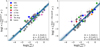Fig. 6 $\log (<L_{\mathrm{a}\mathrm{c}\mathrm{c}}^{lines}>)$ vs. log $L_{\text{acc\hspace{0.17em}}}^{\text{modeling}}$. Colors of the points represent different star-forming regions as described in the legend. The blue line corresponds to our best fit. The dashed black line shows the linear trend as a reference. Left: log < Lacc >lines is computed as the average from the Lacc’s from many lines and using empirical relations by Alcalá et al. (2017) and log $L_{\text{acc\hspace{0.17em}}}^{XS}$ is obtained using the XS-fit method. Right: log < Lacc >lines is computed as the average from the Lacc’s from many lines and using empirical relations obtained in this work and log $L_{\text{acc\hspace{0.17em}}}^{HST}$ is obtained using the HST-fit method.

3.4 L_acc from lines vs. L_acc from modeling

We compared L_acc values derived from direct UV excess modeling (XS- and HST-fit) with those computed indirectly using empirical relations from A17 and this work, respectively (see Sect. 3.3). To ensure consistency, observed fluxes of each accretion tracer were respectively de-reddened using A_V from both XS-fit and HST-fit (Table A.1, applying the Cardelli et al. (1989) extinction law with R_V = 3.1. Line luminosities were then calculated using distances in Table A.1.

For our sample, the $L_{\text{acc\hspace{0.17em}}}^{XS}$ and $L_{\text{acc\hspace{0.17em}}}^{HST}$ values were computed using empirical relations from A17 and our newly derived relations, respectively (Table A.1 for XS; Table 1 for HST). The tabulated log $L_{\mathrm{a}\mathrm{c}\mathrm{c}}^{\text{lines}}$ values are the average of log $L_{\mathrm{a}\mathrm{c}\mathrm{c}}^i$ computed from the several tracers, with errors given as the standard deviation.

Fig. 6 illustrates the log L_acc vs. log $L_{\mathrm{a}\mathrm{c}\mathrm{c}}^{\mathrm{lines}}$ comparison for XS-fit and A17 relations (left panel), and for HST-fit and our relations (right panel). Colors denote star-forming regions. Linear regression fits for both cases, performed as described in Sect. 3.2, show general agreement between UV excess modeled and empirically derived accretion luminosities.

Specifically, the fit for the left panel is: $$\log L_{\mathrm{a}\mathrm{c}\mathrm{c}}^{lines}=(1.0\pm 0.1)\log L_{\mathrm{a}\mathrm{c}\mathrm{c}}^{XS}+(-0.1\pm 0.1)$$(2)

with a standard deviation of 0.02 ± 0.02 and a correlation parameter of 1.0. We found an agreement for the L_acc values within errors for 85% (56/64) of the sources. Of the remainder, 11% (7/64) show higher L_acc up to 0.19 dex via XS-fit, and 4% (3/64) show lower up to 0.37 dex. The log L_acc range differs slightly: −4.49 to 0.17 using the XS-fit, vs. −4.20 to −0.39 using A17 empirical relations.

Similarly, the fit of the right panel is $$\log L_{\mathrm{a}\mathrm{c}\mathrm{c}}^{lines}=(1.0\pm 0.1)\log L_{\mathrm{a}\mathrm{c}\mathrm{c}}^{XS}+(-0.1\pm 0.1)$$(3)

with a standard deviation of 0.05 ± 0.02. 66% (40/61) of the sample shows L_acc agreement within errors. L_acc is higher up to 0.26 dex for 18% (11/61) with HST-fit and lower up to 0.65 dex for 16% (10/61). The log L_acc range is −4.15 to 0.23 when computed using the HST-fit model, vs. −4.15 to 0.65 when computed with corresponding empirical relations.

Using a number of tracers distributed in a wide spectral range improves L_acc estimates (e.g., Rigliaco et al. 2012; Alcalá et al. 2019; Fiorellino et al. 2022a). Thus, we investigated the impact of the Brγ line, our longest-wavelength tracer, which is not always detected (Table A.1). The Brγ line is also known to trace highly accreting CTTS. Repeating the analysis for the subset of sources with detected Brγ only, hereafter referred to as the Brγ-sample, we found no statistical difference in L_acc results, with linear regression fits yielding the same best-fit parameters as Eqs. (2) and (3). Thus, we conclude that in the case of our sample, the L_acc estimate does not depends on the Brγ detection.

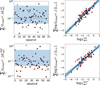Fig. 7 Left panels: fraction of the total luminosity in lines relative to the accretion luminosity, i.e. the continuum excess luminosity. The light blue region corresponds to the range of values found in Alcalá et al. (2014). Right panels: total luminosity from the lines as a function of the log Lacc as indicated in the labels. The blue line in each panel corresponds to our best fit, while the light-blue lines give an indication of the spread of the fit (see Sect. 3.4). The dashed gray lines show the one-to-one relation. Red circled black dots correspond to sources where the Brγ line is detected.

3.5 Continuum excess versus emission in lines

It is interesting to quantify how much energy per unit time is emitted in the continuum relative to that in lines, Σ_iL_lines,i, and whether the Σ_iL_lines,i to L_acc ratio depends on the stellar mass.

We computed the fraction of the total luminosity from the lines, Σ_iL_lines,i, with respect to the accretion luminosity from the continuum excess emission L_acc. For every CTTS, we computed Σ_iL_lines,i as the sum of the luminosity of all the emission lines considered in this work. Fig. 7 shows the results of our analysis. The top panels refer to log $L_{\text{acc\hspace{0.17em}}}^{XS}$ and L_line dereddened using $A_V^{XS}$; while the bottom panels refer to log $L_{\text{acc\hspace{0.17em}}}^{HST}$ and L_line dereddened using $A_V^{HST}$. The blue region on the left panels corresponds to the range of values found for the A17 Lupus sample, i.e. 0.05 < Σ_iL_lines,i/L_acc < 0.55. The range of ratios in our sample is broader than in A17, ranging from 0.01 to 0.69 for ${\mathrm{\Sigma }}_i{L}_{\text{lines}}{}_{{}^{\mathrm{A}17},\mathrm{i}}/L_{\mathrm{a}\mathrm{c}\mathrm{c}}^{XS}$, and from 0.01 to 1.11 for ${\mathrm{\Sigma }}_i{L}_{\text{lines}{}^{\mathrm{T}\mathrm{W}},\mathrm{i}}/L_{\text{acc}}^{HST}$. The panels on the right show Σ_iL_lines,i as a function of accretion luminosity in a log scale. A linear regression fit in this parameter space yields $$\log \left({\mathrm{\Sigma }}_i{L}_{\text{lines\hspace{0.17em}},\mathrm{i}}/{\mathrm{L}}_{\odot }\right)=(0.9\pm 0.1)\times \log \left(L_{\mathrm{a}\mathrm{c}\mathrm{c}}/{\mathrm{L}}_{\odot }\right)-(1.3\pm 0.1)$$(4)

with a correlation factor of 1.0 and σ = 0.14 ± 0.10 for the XS-fit (top right); and $$\log \left({\mathrm{\Sigma }}_i{L}_{\text{lines\hspace{0.17em}},\mathrm{i}}/{\mathrm{L}}_{\odot }\right)=(0.8\pm 0.1)\times \log \left(L_{\mathrm{a}\mathrm{c}\mathrm{c}}/{\mathrm{L}}_{\odot }\right)-(1.5\pm 0.1)$$(5)

with a correlation factor of 0.9 and σ = 0.36 ± 0.16 for the HST-fit (bottom right). This result confirms the correlation between these two quantities, and is consistent with the best fit presented in A17 sample. The fit performed for the Brγ-sample (black dots surrounded by red circles) provides the same results. The dashed lines in the right panels of Fig. 7 show the one-to-one relation. It is interesting to note that the total energy emitted in lines is more similar to that of the continuum at low L_acc values (i.e. tendentially for objects with low masses). However, by plotting log(Σ_i L_lines,i/L_⊙) as a function of the stellar mass, there is no evident correlation.

3.6 Extinction estimates with empirical relations

Previous sections show that empirical relations are a practical tool to compute L_acc. However, these relations can only be applied to the extinction-corrected fluxes. Thus, computing A_V is a key step in measuring L_acc with empirical relations. Our dataset allows us to estimate A_V with a direct modeling of the UV excess, either the XS or the HST fit. However, this is not possible for very noisy UVB data or when the bluest part of the UVB spectrum (λ ≲ 370 nm) is not available. In these cases, the empirical relations can be used to estimate the extinction, provided that a good number of emission line fluxes in the widest possible wavelength range are available.

We adopt three methodologies, independent of the UV excess modelling results, to estimate A_V. These methodologies are based on the assumption that the accretion luminosity, L_acc,i, as derived from different accretion tracers, must be the same for all the lines. Thus, in a plot of log L_acc,i as a function of log λ, the log L_acc,i differences can be minimized with the three adopted methods, yielding a flat log L_acc vs. log λ distribution and the A_V that minimizes the log L_acc,i differences. We used the XS sample only, because we demonstrated that results between XS-fit and HST-fit and their corresponding empirical relations are in agreement and the XS sample contains more sources, enabling a better statistical analysis.

We proceeded as follows: we artificially corrected the observed line fluxes for extinction using a grid of A_V values ranging from 0 to 3 mag, in steps of 0.05 mag. This produces a corresponding grid of line luminosities, which we then used to derive a grid of accretion luminosities (L_acc) through the empirical relations.

The three adopted methods to minimize the $L_{\mathrm{a}\mathrm{c}\mathrm{c}}^{\text{lines}}$ differences as a function of wavelength are:

• weighted coefficient method, $A_V^W$: selecting the A_V that minimizes the slope of the L_acc vs. log λ relation, using 1/Δ log L_acc as the weight of each point;

• unweighted coefficient method, $A_V^{\text{notW}}$: same as the previous method but without weighting for uncertainties;

• difference method, $A_V^{\text{diff}}$: selecting the A_V that minimizes the dispersion among log L_acc values (including their error) derived from different accretion tracers.

The results of these methods are graphically shown in the top panels of Fig. 8: the left and central panels display the coefficient methods with and without weighting, respectively, while the right panels present the difference minimization method. The extinction values derived with the three approaches differ (see Table 1). To evaluate the accuracy of these methods, we compared the derived A_V values with $A_V^{\mathrm{X}\mathrm{S}}$, using it as a benchmark. The distribution of $A_V^{\mathrm{X}\mathrm{S}}$ vs. $A_V^{\text{lines}}$ is broad in all three cases and does not show a clear linear trend. More in detail, the root mean square (rms) deviation between $A_V^{\mathrm{X}\mathrm{S}}$ and A_V is 0.8, 0.5, and 0.4 for the weighted, unweighted, and difference methods, respectively. As anticipated in Sect. 3.2, the result is the same between $A_V^{\mathrm{H}\mathrm{S}\mathrm{T}}$ and $A_V^{\mathrm{d}\mathrm{i}\mathrm{f}\mathrm{f}}$ (see the right panel of Fig. 4).

We computed the line luminosity and accretion luminosity as described in Sect.3.4 using the extinction values provided by the above three minimizing methods. The bottom panels of Fig. 8 show the linear regression performed as described in Sect. 3.2 between the accretion luminosity obtained from the XS-fit and the accretion luminosity obtained from accretion tracers luminosities calculated with the tree different A_V values. The relations found for the three methods are: $$\log L_{\mathrm{a}\mathrm{c}\mathrm{c}}^{lines-W}=(0.8\pm 0.1)\log L_{\mathrm{a}\mathrm{c}\mathrm{c}}^{XS}+(-0.0\pm 0.2)$$(6) $$\log L_{\mathrm{a}\mathrm{c}\mathrm{c}}^{lines-notW}=(0.8\pm 0.1)\log L_{\mathrm{a}\mathrm{c}\mathrm{c}}^{XS}+(-0.6\pm 0.2)$$(7) $$\log L_{\mathrm{a}\mathrm{c}\mathrm{c}}^{lines-diff}=(1.0\pm 0.1)\log L_{\mathrm{a}\mathrm{c}\mathrm{c}}^{XS}+(-0.2\pm 0.1)$$(8)

with a standard deviation of 0.2, 0.1, and 0.1, respectively, and a correlation factor of 0.9 in all three cases. Only the best fit obtained with the difference-method (Eq. (8), low right panel in Fig. 8) is consistent with the one-to-one line within the error. We conclude that the difference-method yields an A_V value which best reproduces the accretion luminosity distribution from the XS modeling.

Appendix E shows the log L_acc vs. log λ plots for the PENELLOPE sample. Those plots show the comparison of the log L_acc when using the $A_V^{XS}$ and $A_V^{diff}$ values to correct the line fluxes for extinction. Fig. 9 shows two examples of these plots. The top panel shows the case of the triples system VW Cha, while the bottom panel shows the case of SO1153 young star. For VW Cha, the difference method and the XS-fit provide consistent results of A_V and L_acc. Thus, the distribution of log L_acc vs. λ is flat in both the cases, as in the 80% of the sources in our sample (see Appendix E). Differently, applying the difference method to SO1153 YSO, we find $A_V^{diff}\ne A_V^{XS}$, this happens in 20% of the sources in our sample. In this case, the log L_acc vs. λ distribution appears flatter when using one of the two methods (XS-fit or difference method), compared to the other. We discuss this further in Sect. 4.

We note that in some sources the Brγ line provides systematically lower (0.5 dex on average) L_acc values with respect to the average drawn from the many other lines. This could be attributed to photospheric line contamination, especially for sources with weak Brγ emission. This aligns with the observation that consistent results are obtained for objects displaying strong Brγ emission in our sample. Furthermore, uncertain K-band flux calibration is a non-negligible potential source of this discrepancy.

To identify the shortest wavelength range that provides A_V values consistent with $A_V^{diff}$, computed using all accretion tracers from the UVB to the NIR, we performed several checks. We analysed if and how much the $A_V^{diff}$ estimate changes considering only UVB tracers (emission lines up to 600 nm), only VIS tracers (emission lines with 600 nm < λ < 900 nm), only NIR tracers (λ > 900 nm), and combination of these bands. For this analysis we selected only the Brγ sample. We found that the difference method fails when using only one band. Contrary, extinction estimates using UVB+VIS bands yield results consistent with the $A_V^{\text{diff}}$. When considering UVB + NIR or VIS + NIR tracers, the $A_V^{\text{diff}}$ is underestimated in 80% of the cases. We believe this is related to the fact that, when detected, the Brγ line often yields log L_acc values lower than those derived from other lines (see Figs. in Appendix E).

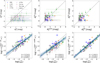Fig. 8 Top panels: comparison between $A_V^{XS}$ and the extinction drawn from the coefficient method without weights (left), the method weighting for the error (central), and the difference method. Lower panels: comparison between average Lacc computed with the three methods and $L_{\mathrm{a}\mathrm{c}\mathrm{c}}^{XS}$. The blue line corresponds to the best fit.

3.7 Brackett series

Similarly to Balmer and Paschen series, the Brackett, Pfund, and Humphreys series lines are believed to trace the accretion process. These lines link the NIR with the mid-infrared (MIR) and far-infrared (FIR) regions and could, in principle, serve as calibrators for the JWST data (Salyk et al. 2013; Rigliaco et al. 2015; Rogers et al. 2024; Tofflemire et al. 2025).

The PENELLOPE sample contains objects where several lines of the Brackett series were detected, differently to the A17 Lupus sample where only two objects were found to display Brackett series lines. In particular, we investigated the correlation between $L_{\text{acc\hspace{0.17em}}}^{XS}$ and L_line among Brackett lines higher than Brγ (Br7), namely, lines from Br8 to Br21.

We measured the line fluxes of these lines as described in Appendix C and computed line luminosities in the same way as for the other permitted lines. We then plot the result of the lines luminosity with the corresponding accretion luminosity, $L_{\mathrm{a}\mathrm{c}\mathrm{c}}^{XS}$ or $L_{\mathrm{a}\mathrm{c}\mathrm{c}}^{HST}$. Figs. F.1 and F.2 in Appendix F show the correlation between log L_acc and log L_{Br line} for a few of these lines. We can appreciate a qualitative correlation, which suggests that these lines trace, indeed the accretion process, but the number of non-detections (upper limits plotted as triangles) is generally high and, in most cases, higher than the detections, making difficult to draw definitive conclusions.

We decided to fit this type of correlation only for diagnostics that have been detected in at least ten sources (i.e., Br10, Br11, and Br13). The fit has been done using the hierarchical bayesian method from Kelly (2007), as described in Sect. 3.2. The best fit of these lines is shown in Table F.1. We note that the correlation factor is between 0.6 and 0.8, suggesting moderate correlation between these Br-series lines and the accretion luminosity. The slope and intercept of the Br13 is in agreement when computed using the PENELLOPE and the ODYSSEUS samples. In contrast, the Br11 and Br10 relation changes significantly when using the two samples. This suggests that, considering the sources in our sample, the Br11 and Br10 relations are not well constrained. In general, we stress that the fit we performed suffers from uncertainties due to the low statistics (N_points = 11 or 12 for the Br13 and Br11 lines), the possible contamination of photospheric lines, and more importantly the modest range amplitude in line luminosity, hence, accretion luminosity.

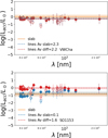Fig. 9 log Lacc as a function of the wavelength for two PENELLOPE CTTSs. Filled (empty) circles are log Lacc values computed using empirical relations, corresponding to suggested (non suggested) lines by Alcalá et al. (2014), while triangles represent upper limits. In red and blue results obtained by dereddening the flux with $A_V^{diff}$ and $A_V^{XS}$ are shown, respectively. Horizontal red and blue dashed lines and regions correspond to mean value and standard deviation of Lacc using $A_V^{diff}$ and $A_V^{XS}$, respectively. The orange solid line shows $L_{\text{acc\hspace{0.17em}}}^{XS}$ with its error bar (orange horizontal region). Top: plot for the multiple system VW Cha, where the extinction and accretion luminosity estimated with the difference method and the XS-fit are in agreement and the log Lacc distributions are flat. Bottom: SO1152 young star, where $A_V^{diff}$ and $A_V^{XS}$ differ by 1.5 mag and the distribution of log Lacc obtained by dereddening the fluxes with $A_V^{diff}$ is flatter than the one obtained using $A_V^{XS}$. The latter increases with the wavelength.

4 Discussion

4.1 Empirical relations for CTTS

Fit results shown in Eqs. (2) and (3) indicate that the relations between log L_acc modeled from UV excess and the corresponding log $L_{\mathrm{a}\mathrm{c}\mathrm{c}}^{\mathrm{lines}}$ is linear, suggesting that empirical relations can generally be used to estimate L_acc. Remarkably, our sample is composed of CTTSs from various star-forming regions, including OB1 and σOri. These regions host both a low-mass population of CTTS and massive O- and B-type stars, which emit intense UV radiation capable of inducing external photoevaporation in CTTS disks (Rigliaco et al. 2009; Maucó et al. 2023, 2025). We also stress that the recent work by Halstead Willett et al. (2025), based on a Bayesian approach to derive L_acc, demonstrates that the log L_acc − log L_line relations of objects in more distant regions like Serpens, IC5146, NGC7000, etc, are in agreement with the previous results by A17. All this shows that the log L_acc − log L_line empirical relations can be applied in a variety of star forming environments (see Fig. 6).

It is, however, important to bear in mind that not all accretion tracers correlating with L_acc are equally reliable for constraining L_acc, due to poor statistics, blending of lines, or contributions from mechanisms like winds, as observed for Hα or the HeI line at 1082.9 nm (this latter line is not included in our analyses because of its complexity, see Edwards et al. 2006). Likewise, H7, HeI FeI, CaII(H), and OI at 777.30 nm are blended with other species and should also be used with caution in computing L_acc. For the remaining accretion tracers, we examined the correlation factor and spread of our empirical relations, with a higher correlation factor and a lower spread indicating a more reliable relation to estimate L_acc. Table D.1 shows that all tracers have correlation factors above between 0.8 and 1.0. However, Fig. 5 shows that the empirical relations revisited with the HST-ULLYSES data, which provide more UV information than X-shooter, are in agreement with previous versions for most tracers. Contrary, the He I at 471.31 nm, the OI at 844.64 nm, and the Pa 10 are not in agreement within 2σ with the A17 relation coefficients. These lines, when used alone, could provide uncertain values of L_acc.

We also emphasize that different lines form in distinct regions within the accretion columns (see for example the review by Hartmann et al. 2016). Narrow components, such as Paschen series lines, generally form in the postshock region near the stellar surface, whereas broad components, such as Balmer series lines, usually form in the pre-shock region. Consequently, different lines may suit specific regions of interest, but characterizing the overall accretion luminosity demands incorporating the highest possible number of lines tracing both pre-shock and post-shock regions.

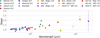Fig. 10 Slopes of empirical relations of Alcalá et al. (2017) sample (filled circles), this work (filled stars), and from the literature (Salyk et al. 2013; Rigliaco et al. 2015; Komarova & Fischer 2020; Rogers et al. 2024; Tofflemire et al. 2025, filled squares), as a function of the wavelength. Error bars are smaller than the symbols when not visible.

4.2 The Brackett series

We also provide Br-series relations for the Br10, Br11, and Br13 lines. The coefficients of the Br13 line obtained using the XS- and the HST-fit are in agreement, while the coefficients of the Br10 and Br11 lines are not. This might be due to the limited line luminosity range of the Br10 and Br11 (−5.2 < log L_Br10 < −3.5, −5.8 < log L_Br11), compared to the wider luminosity range of the Br13 (−7 < log L_Br10 < −3.8). Further investigation of other sources with the same techniques will improve the statistics, providing stronger results.

The tentative slopes of the Br-series that we computed with the PENELLOPE sample are between 1.3 and 1.0, steeper than the optical and NIR slopes, ranging between 0.8 and 1.3 (see Table D.1). Fig. 10 shows the correlation slopes as a function of the wavelength. Different colors trace different elements and specific HI lines as described in the legend. We followed up the analysis by Tofflemire et al. (2025), where a trend in the slope as a function of the energy level of the hydrogen series has been found. These authors have speculated that this type of increasing trend could be due to the fact that hydrogen at different excitation levels come from different physical conditions (such as temperature and density); thus, different lines trace the pre-shock region in different part of the accretion column or the post-shock region.

In the analysis slopes of the empirical relations, we incorporated Pfβ (Salyk et al. 2013), Huβ (Rigliaco et al. 2015), Brα (Komarova & Fischer 2020), Paα and Brβ (Rogers et al. 2024). The increasing trend suggested by Tofflemire et al. (2025) is less convincing when including the latter tracers, since we note a large spread in the distribution, which increases with the wavelength. However, fitting the slopes distribution as a function of their wavelength, we find a correlation factor of 0.9. It must be stressed that, while Tofflemire et al. (2025) compared slopes obtained by computing the accretion luminosity using the XS-fit model from X-shooter data (which can therefore be directly compared to all the slopes up to Br10) other empirical relations have been derived using different approaches to estimate L_acc, and may consequently introduce systematic biases. More specifically, the empirical relations from the literature (Salyk et al. 2013; Rigliaco et al. 2015; Komarova & Fischer 2020) were fitted using L_acc estimates that are not contemporaneous with the line flux measurements. Moreover, the line luminosity ranges used to fit the Pfβ, Hγ, Hβ, and Hα relations are very narrow (e.g., −4.2 < log L_Paβ < −3.2 for Pfβ, and −1.5 < log L_H < 0 for the other H-lines; Salyk et al. 2013; Tofflemire et al. 2025). We also add that the low resolution of Spitzer and the delicate subtraction of H₂O also affect the MIR empirical relations (Baskaran et al., in prep.). Finally, Rogers et al. (2024) analysed a sample of CTTSs in a low-metallicity environment and derived their best-fit relations for Paα and Brβ by computing L_acc indirectly from the Brγ line using the A 17 relation.

All the differences in terms of methodology, sample selection, and luminosity range: (i) contribute to the spread observed in the slope −λ distribution; (ii) affect the uncertainties in the empirical relations themselves, including the slope values. Only simultaneous observations of UV excess and MIR accretion tracers of CTTSs with a suitable luminosity range will enable the determination of accurate empirical relations to link the accretion luminosity to the MIR accretion tracers.

4.3 Considering the A_V estimate

A critical aspect in analyzing accretion values and applying empirical relations is the estimate of A_V. Our results show that different approaches provide different results with a non-negligible spread (0.4–0.5) with no linear trend. Curiously, this is also valid for the extinction provided from two direct modeling of UV excess, namely, the XS-fit and the HST-fit (see Fig. 4). It is possible that the spread in the A_V estimate is at least partially responsible for the spread in the log $L_{\mathrm{a}\mathrm{c}\mathrm{c}}^{HST}$ − log $L_{\mathrm{a}\mathrm{c}\mathrm{c}}^{XS}$ distribution (Fig. 3). We note here that the accretion luminosity from the HST-fit is not necessarily higher than the one provided by the XS-fit, as one would expect (Pittman et al. 2022) given the much extended UV spectral range of HST with respect to X-shooter (Alcalá et al. 2019). The spread in the distribution of both the extinction and the accretion luminosity computed with the XS- and HST-fit suggests intrinsic uncertainty within which it is possible to estimate these parameters, using the PENELLOPE and ODYSSEUS methods.

Among the three different approaches to estimate A_V based on empirical relations, one is more reliable than others (Sect. 3.6). Indeed, the rms between the $A_V^{XS}$ and the extinction calculated by each method is lowest for the difference method (0.4), indicating that $A_V^{diff}$ estimates are the most similar to $A_V^{XS}$. This is also the spread present when comparing $A_V^{diff}$ and $A_V^{XS}$ with $A_V^{HST}$, suggesting 0.4 as a possible estimate of the intrinsic extinction uncertainty.

Eq. (8) shows that using $A_V^{diff}$ to deredden the line fluxes results in a linear correlation between $L_{\mathrm{a}\mathrm{c}\mathrm{c}}^{XS}$ and $L_{\mathrm{a}\mathrm{c}\mathrm{c}}^{\mathrm{lines}}$. This implies that when A_V is computed from observed line fluxes using the difference method, the L_acc derived through A17 empirical relations matches that obtained from the XS-fit. However, we point out that A_V is constrained only when simultaneously observed accretion tracers span a broad wavelength range, ideally from the UVB to the NIR.

We also found that in 80% of our sources (51/64), the L_acc values derived using empirical relations and dereddening the line fluxes with both $A_V^{XS}$ and $A_V^{diff}$ are consistent (see Appendix E). For the remaining 20%, the extinction estimate differs by at least 0.5 mag within the error, where 0.5 mag is the typical error on $A_V^{XS}$ but, on the other hand, very similar to the spread of 0.4 mag that we found when comparing the XS-fit, the HST-fit, and the difference method estimates. In these cases, the slope of the log L_acc distribution as a function of the wavelength is flatter for 5 sources (SO1153, Sz66, Sz76, Sz98, Sz129) when using $A_V^{diff}$ to deredden the fluxes, suggesting this is a best extinction estimate for these objects. On the contrary, for 6 sources (CVSO90, CVSO176, Sz10, CVSO165, Sz130) the same distribution is flatter when using $A_V^{XS}$ to deredden the fluxes, thus $A_V^{XS}$ seems to be the best extinction estimate (see Appendix E).

This analysis confirms that measuring the extinction on YSOs can be challenging, even with the established methods like the XS- or HST-fit. Alternative approaches, using Bayesian methods (Halstead Willett et al. 2025), may yield more reliable results. Instead of providing a single best-fit value with an associated error, Halstead Willett et al. (2025) method treats all stellar and accretion properties as probability distributions. It combines prior information with the observed spectral data to generate a posterior probability distribution for the parameters, using Monte Carlo Markov chain techniques. This approach’s main advantage is its ability to simultaneously explore the entire parameter space of the accretion model, allowing for a more robust characterization of all uncertainties and a direct measurement of the correlations between different parameters, although degeneracies among fit parameters cannot always be removed. Our analysis also demonstrates that it is possible to estimate A_V yielding accretion results in agreement with those of the XS-fit, but using empirical relations alone.

Notably, comparing log $L_{\text{acc\hspace{0.17em}}}^{XS}$ and log $L_{\text{acc\hspace{0.17em}}}^{HST}$ we also find a nonnegligible spread (see Fig. 3). Indeed, L_acc is used to estimate the mass accretion rate (${\dot{M}}_{\text{acc}}$), which plays a key role in constraining the processes responsible for disc evolution in population synthesis models (e.g., Manara et al. 2023). Typically, published studies (e.g., Lodato et al. 2017; Mulders et al. 2017; Tabone et al. 2022; Somigliana et al. 2023) assume a systematic uncertainty on ${\dot{M}}_{\text{acc}}$ of 0.45 dex on the values obtained fitting the UV excess with X-shooter. It would be important to understand whether this assumed uncertainty value is to be revised in light of the differences between log $L_{\text{acc\hspace{0.17em}}}^{HST}$ and log $L_{\text{acc\hspace{0.17em}}}^{XS}$ found combining the HST and X-shooter spectra from ULLYSES and PENELLOPE. Further investigation is needed to understand the reason of the differences observed in this work, and we will discuss this topic in a forthcoming paper.

4.4 Using empirical relations for other types of YSOs and forming-planets

Empirical relations for accretion have been applied not only to CTTSs but also to younger YSOs, including Class I and Flat Spectrum (FS) objects (i.e., Fiorellino et al. 2021, 2023; Delabrosse et al. 2024; Tychoniec et al. 2024), as well as to eruptive YSOs (e.g., Hodapp et al. 2020; Siwak et al. 2023; Singh et al. 2024; Fiorellino et al. 2024; Giannini et al. 2024), to accreting brown dwarfs (e.g., Whelan et al. 2018; Almendros-Abad et al. 2024), and even on planets (e.g., Plunkett et al. 2025; Bowler et al. 2025). However, since these relations were derived for CTTSs, their application to other types of objects, which may accrete through different mechanisms, requires some examination. According to Mendigutía et al. (2015) the empirical relations between log L_acc and log L_line are a direct consequence of the log L_acc − log L_⋆ correlation. Therefore, the log L_acc − log L_line relations are not necessarily related with the physical origin of the lines. However, it is essential to verify this paradigm in YSOs beyond CTTS.

Recent findings by Flores et al. (2024) show that Class I and FS objects have magnetic field comparable to those of Class II YSOs. This suggests that magnetic fields, responsible for accretion on CTTSs, could play the same role also in Class I and FS objects, supporting the use of empirical relations for Class I and FS sources. However, some caveats exist. The first relates to the presence of veiling (r), representing the excess emission above the photosphere. Embedded YSOs, such as Class I and FS, often exhibit high veiling (r ~ 50), unlike CTTS (r < 2). For this reason, it is crucial to take into account the effect of the veiling before applying empirical relations in Class I, FS, or earlier-phase YSOs. Accurate veiling correction is challenging but vital, as it can significantly impact L_acc estimates despite the empirical relations’ accuracy. The second caveat stems from Class I and FS being embedded in their envelopes, thus obscuring their UV and optical emission and limiting their study to longer wavelengths. Paβ and Brγ are commonly used to estimate L_acc, and our results show that all the high accretors in our sample exhibit Paβ and Brγ in emission, providing L_acc luminosity in agreement with other accretion tracers. Thus, assuming Class I and FS are younger than CTTSs and should be high-accretors (log L_acc > −1), the use of NIR empirical relations becomes a powerful tool to constrain accretion luminosity during the protostellar stage. However, using only NIR accretion tracers could underestimate the accretion luminosity (Harsono et al. 2023) because most of the magnetospheric emission is completely blocked from view, and line fluxes are only catching a tiny fraction of L_acc through scattered light on the (less extincted) cavity walls (Delabrosse et al. 2024). Thus, we agree with the conclusion of Delabrosse et al. (2024) that more complex methodologies should be used to constrain L_acc on Class I to fully correct for occultation of the central source, and of the associated NIR emission. This is, for example, the case of the self-consistent approach used in Antoniucci et al. (2008); Fiorellino et al. (2021, 2023), based on empirical relations, integrated with the use of isochrones (or birthline) and bolometric luminosity and veiling measurements. We also highlight that the samples of Class I protostars in both Fiorellino et al. (2023) and Flores et al. (2024) are limited to those with high S/N values, while fainter Class I objects (m_K < 15) have not been analyzed yet.

In the case of episodic accretion, FUors event fall outside magnetospheric accretion (e.g., Audard et al. 2014; Vorobyov & Elbakyan 2020), so empirical relations should not apply. For EXor-like YSOs, however, the spectral features are very similar to CTTSs ones. More in detail, empirical relations can be used to estimate L_acc in the quiescent phase, when EXors accrete similarly to CTTSs, but not during the bursts. Indeed, Cruz-Sáenz de Miera et al. (2023) show that, during the last burst of Ex Lupi, L_acc obtained with the XS-fit is up to one order of magnitude different than the L_acc computed using A17 empirical relations, higher or lower depending on the studied epoch. This result suggests that empirical relations obtained from CTTSs might not be applied to study EXors bursts.

Other cases where empirical relations have been applied are those of brown dwarfs (BDs) and forming planets, whose faintness in the UV often prevents direct UV excess modeling of the data. Mohanty et al. (2005) showed that the CTTS-like accretion paradigm can be extended down to BDs with masses as low as ~15 M_J. This result has been confirmed by numerous other studies, and it is now widely accepted that stars and BDs share a common dominant formation mechanism (see review by Chabrier et al. 2014). Also, Reiners & Basri (2007) directly measured strong magnetic fields in BDs, on the order of kilogauss, demonstrating that BDs can generate fields comparable in strength to those of CTTSs. These results suggest that empirical relations provide reliable accretion luminosity estimates for BDs.

The situation is less clear for giant planets. Direct magnetic field measurements for exoplanets are still lacking, and observations of solar system planets set the maximum field strengths at only a few gauss (4–14 G) (Connerney et al. 2018). However, models suggest that hot Jupiters could have significantly stronger surface magnetic fields. For instance, Cauley et al. (2019) estimated that hot Jupiters could have surface magnetic fields ranging from 20 to 120 G, 10 to 100 times stronger than those observed in the solar system and comparable to CTTS values for the stronger cases. Nevertheless, unlike in CTTSs, magnetic fields are not believed to be the primary driver of accretion in giant planets. Core accretion is thought to proceed without the need for strong magnetic coupling, although magnetic fields may influence the dynamics of the surrounding disk (Turner et al. 2014). Thus, even if forming planets may possess strong magnetic fields, it remains unclear whether a magnetospheric accretion scenario applies. Recent works reported hints of physical conditions compatible with magnetospheric accretion scenario in a few cases (Ringqvist et al. 2023; Viswanath et al. 2024). Due to the limited number of observed accreting planets, a systematic study to probe magnetopheric accretion as the general and main mechanism to build the planetary mass is still missing. Consequently, the reliability of accretion luminosity estimates based on empirical relations in the planetary regime is still uncertain.

4.5 Total energy emitted in lines versus in continuum

In a recent work, Hashimoto & Aoyama (2025) studied 76 brown dwarfs and very-low mass stars by assuming the magnetospheric accretion model, that is, using empirical relations from A17, and the accretion-shock model, namely, using empirical relations from Aoyama et al. (2021) initially created for accreting planets. The difference between the magnetospheric accretion and the accretion-shock model is that the first assumes that accretion tracers such as hydrogen lines primarily come from the accretion flow, while the latter assumes they come from the shock region. They found a bimodal trend between the energy per unit time emitted from the lines E_lines = ΣL_lines,i and the energy per unit time emitted from the continuum, E_cont = L_acc, when using empirical relations from Aoyama et al. (2021), while it confirms the presence of a correlation between E_lines and E_cont, even for very-low mass objects, when using empirical relations from A17. In particular, they found E_lines ~ E_cont for very-low mass objects, while they reported E_cont >> E_lines for the more massive objects (see also Zhou et al. 2021).

In our CTTSs sample, Eqs. (4) and (5) (see also right panels of Fig. 7) indicate the trend that objects with lower L_acc tend to emit energy in lines close to that of the continuum. Given that low-L_acc objects are typically less massive, this raises questions about the behavior of the E_lines/E_cont ratio in progressively less massive objects, such as sub-stellar and planetary-mass objects. The comparison between Hashimoto & Aoyama (2025) and this work results suggests that the trend we note in our sample continues in the very-low mass regime, but according to the analysis by Hashimoto & Aoyama (2025), the trend is different if the shock model is at work in planetary-mass objects. We also note that for lower accretors, the contribution from chromospheric emission could account for a significant fraction of the measured line flux and may explain the trend observed in Fig. 7. To perform a direct comparison between young stars and planetary-mass objects (e.g., from Hashimoto & Aoyama 2025), it would be necessary to subtract this chromospheric contribution from the accretion tracer lines. However, as it is highly challenging to account for this contribution precisely, we emphasize that any such comparison must be interpreted carefully in light of this caveat.

5 Conclusions

In this study, we analyzed 64 X-shooter spectra of CTTSs from the PENELLOPE sample. For 61 of these CTTSs, we also used quasi-contemporaneous HST spectra. We showed that the accretion luminosities derived with the HST-fit and XS-fit methods are statistically consistent, although significant differences can arise for individual objects.

By revisiting the log L_acc−log L_line empirical relations using accretion luminosities computed via HST modeling and the HST-ULLYSES data, we confirmed the robustness of most of the relations derived from X-shooter data. We also conclude that empirical relations are valid for regions in various environments. The spread in the extinction and accretion luminosity values derived with the two approaches suggest the existence of an intrinsic uncertainty in our current estimates of these paramenters.

We also present a “difference method” based on empirical relations as an independent way to constrain extinction in CTTSs. This method yields A_V values comparable to those obtained via the XS-fit, along with a similar distribution of accretion luminosities.

We highlight that for all the high-accretors (13 CTTS), we detected NIR tracers such as Paβ and Brγ, with their fluxes yielding accretion luminosity estimates similar to the XS-fit. For low accretors (log $L_{\mathrm{a}\mathrm{c}\mathrm{c}}^{XS}<-1$) with a Brγ detection (37 CTTSs in our sample), the NIR lines luminosities underestimate the accretion luminosity of 0.5 dex (on avarage) in 51% of the sources (19/37). This suggests that under the assumption of being high-accretors, L_acc can be reliably estimated using Paβ and Brγ. This is particularly useful to constrain L_acc on embedded sources not accessible at UVB or VIS bands, such as Class I YSOs. In general, log L_acc − log L_line empirical relations can be applied to Class I and FS protostars, provided that veiling is accurately measured and multiple accretion tracers are used. Accretion studies of eruptive YSOs, particularly EXor-type objects, can also be investigated with these relations during their quiescent phases, when their accretion resembles that of CTTSs. Similarly, empirical relations provide reliable accretion luminosity estimates for brown dwarfs, while their applicability to accreting planets remains unclear.

Data availability

Table 1 is available at the CDS via https://cdsarc.cds.unistra.fr/viz-bin/cat/J/A+A/704/A42

Acknowledgements

In Memoriam of Will Fischer, a pillar of the PENELLOPE-ODYSSEUS-ULLYSES collaboration and the star formation community. His scientific contributions and friendship will be greatly missed. We thank Dr. G. Inchingolo for his assistance with the graphical design of Fig. 1, and Dr. A. Banzatti, Dr. J. F. Gameiro, and Dr. Gabriel-Dominique Marleau for the interesting discussion and feedback about the results of this work. We also thank the anonymous referee for their work to improve this manuscript. This work has been financially supported by Large Grant INAF-2022 “YSOs Outflows, Disks and Accretion: towards a global framework for the evolution of planet forming systems (YODA)”, by Large Grant INAF-2024 “Spectral Key features of Young stellar objects: Wind-Accretion LinKs Explored in the infraRed (SKYWALKER)”, and by the European Union (ERC, WANDA, 101039452). Views and opinions expressed are however those of the authors only and do not necessarily reflect those of the European Union or the European Research Council Executive Agency. Neither the European Union nor the granting authority can be held responsible for them. This work was supported by HST AR-16129 and benefited from discussions with the ODYSSEUS team, https://sites.bu.edu/odysseus/. This work received funding from the Hungarian NKFIH project No. K-147380; by the NKFIH NKKP grant ADVANCED 149943, the NKFIH excellence grant TKP2021-NKTA-64. Project no. 149943 has been implemented with the support provided by the Ministry of Culture and Innovation of Hungary from the National Research, Development and Innovation Fund, financed under the NKKP ADVANCED funding scheme. E.F. has been partially supported by project AYA2018-RTI-096188-B-I00 from the Spanish Agencia Estatal de Investigación and by Grant Agreement 101004719 of the EU project ORP. J.M.A. acknowledges support from PRIN-MUR 2022 20228JPA3A “The path to star and planet formation in the JWST era (PATH)” funded by NextGeneration EU and by INAF-GoG 2022 “NIR-dark Accretion Outbursts in Massive Young stellar objects (NAOMY)”. E.F. and J.M.A. acknowledge support from the INAF MiniGrant 2023 “Investigating the planet formation: initial conditions through the mass accretion rate on protostars”. C.V.P. acknowledges funding from the NSF Graduate Research Fellowship Program under grant No. DGE-1840990. G.L. acknowledges support from PRIN-MUR 20228JPA3A and from the European Union Next Generation EU, CUP:G53D23000870006.

References

Appendix A Sample

Appendix B HST and X-Shooter quasi-simultaneous observations

Despite efforts to coordinate VLT/X-Shooter and HST observations, the datasets are not always perfectly simultaneous. Looking at the time difference between the XS and HST observations (see Table 1), we find that 38% (23/61) of the sources were observed on the same day, 53% (32/61) within two days, 64% (39/61) within one week, 72% within one month, and 80% (49/61) within one year. Sources with a time separation on the order of a year (or larger) correspond to HST archival observations.

Since Fig. 3 shows some scatter in the distribution, we investigated whether this could be related to the time difference between the XS and HST observations. In principle, due to the intrinsic variability of YSOs and the fact that this is expected to be larger after a few days (e.g., Costigan et al. 2014), targets observed closer in time are expected to yield more consistent log L_acc estimates when derived from the XS or HST fits. Conversely, outliers in the distribution may correspond to targets with larger temporal offsets between the two observations. Nevertheless, Fig. B.1 shows no clear trend between the time separation of the observations and the difference in log L_acc estimates using the XS- and HST-fit. To quantitatively verify this, we re-examined the observed scatter by excluding sources with time lags greater than one week. The recomputed scatter (σ) is 0.46, which remains very similar to the original value of 0.50 that includes all sources. The number of sources falling outside the new 1σ range is now 7, which accounts for approximately 17% of this new sample (39 sources). This is comparable to the 9 sources (about 15%) that fell outside the 1σ range in the original, larger sample (61 sources). We would expect to find the agreement between the two measurements to improve. On one hand, the spread slightly decreases, while, on the other hand, the percentage of “outliers” increases. We interpret this finding as further evidence that temporal variability is not the primary source of the spread in the log $L_{\text{acc\hspace{0.17em}}}^{HST}$ vs. log $L_{\text{acc\hspace{0.17em}}}^{XS}$ distribution. We will investigate other possible sources of this scatter in a forthcoming paper.

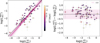Fig. B.1 Comparison of Lacc as in Fig. 3. The colored bar shows the difference in time between XS and HST observations for each target.

Appendix C Measuring the flux of the accretion tracers

The observed flux (F_obs) for the accretion tracers in every CTTS spectrum of the PENELLOPE sample were measured. The procedure was as follows: the local continuum was fitted with a linear function over a wavelength range of Δλ = 2 nm, centered on the emission line’s wavelength λ₀. This range was adjusted, as necessary, based on the line’s intensity and to avoid overlapping emission lines or residual telluric absorption features. The line flux was then obtained by subtracting the local continuum and integrating over the emission line.

The noise of the line was calculated by multiplying the standard deviation of the local continuum (rms) by the wavelength element between two pixels (Δλ), and by the square root of the number of pixels within the wavelength range (N_pix). A line was considered detected if its S/N > 3. For non-detections, upper limits were computed using the following relation, $$F_{line}^{upp}=3\times (\sqrt{N_{pix}}\times rms\times \mathrm{\Delta }\lambda )$$(C.1)

As a reference, we used the same accretion tracers studied in A17. Contrary to the latter, and other previous CTTS X-Shooter samples, PENELLOPE includes several objects in which many lines of the Brackett series have been detected, as the PENELLOPE sample includes a larger number of high accretors with respect to the A17 sample. Hence, we also measured the flux of several of those lines. Observed line fluxes before extinction correction are available on-line on Zenodo⁷.

Appendix D log L_acc vs. log L_line using L_acc from the HST modeling

Figures D.1 and D.2 show the relationships between the accretion luminosity and the line luminosity for several accretion tracers as labelled in each panel.

For each source, we dereddened the observed fluxes of X-Shooter accretion tracers (as listed in Table B.1 of Alcalá et al. 2017) using extinction values derived from the HST-fit (${\mathrm{A}}_V^{HST}$; see Table 1) and applying the Cardelli et al. (1989) extinction law with R_V = 3.1. From the dereddened fluxed, the line luminosity of each accretion tracer was then computed as L_i = 4πd²F_i, where d is the distance of each source as listed in Table A.1.

Each line luminosity was then plotted as a function of the accretion luminosity derived from HST (see Figs. D.1 and D.2) for all the sample. We fit our data by employing the hierarchical Bayesian method from Kelly (2007), which accounts for errors on both axes. To directly compare our results with the ones from A17, we do not include in the fit upper limits. The resulting relation is $$\log L_{\mathrm{a}\mathrm{c}\mathrm{c}}^i=a_i\log L_{\mathrm{a}\mathrm{c}\mathrm{c}}^{HST}+b_i$$(D.1)

where “i” denotes the i-th line. Coefficients are listed in Table D.1.

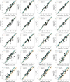Fig. D.1 log Lacc − log Lline and best fit for the Balmer series, the Paschen series and the Brγ line. The blue and orange lines show out best fit and the best fit from Alcalá et al. (2014), respectively. The wavelength in nanometers of each line is shown on the x-axis. Triangles are upper limits.

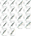Fig. D.2 log Lacc − log Lline and best fit for the helium, calcium, sodium, and oxygen accretion tracers. The blue and orange lines show our best fit and the best fit from Alcalá et al. (2017), respectively. The wavelength in nanometers of each line is shown on the x-axis. Triangles are upper limits.

Appendix E $L_{\text{acc\hspace{0.17em}}}^{\text{lines}}$ as a function of wavelength for the PENELLOPE sample

Figures E.1 to E.4 display the accretion luminosity as a function of the wavelength for every target in the PENELLOPE sample. More in detail, the horizontal orange line represent the log $L_{\text{acc\hspace{0.17em}}}^{XS}$ value; the blue dots correspond to the log $L_{\text{acc\hspace{0.17em}}}^{\text{line,}\mathrm{i}}$ dereddening the fluxes with $A_V^{XS}$ and using the A17 empirical relations and the horizontal blue line is their average value; the red dots correspond to the log $L_{\text{acc\hspace{0.17em}}}^{\text{line,}\mathrm{i}}$ dereddening the fluxes with $A_V^{diff}$ and using the A17 empirical relations and the horizontal red line is their average value.

The sources can be classified into three groups based on plots in Figs. E.1 to E.4. The largest group, comprising 80% (51 out of 64) of our sources, shows an agreement between the three accretion luminosities (see the caption in Fig. E.1) within the errors. For these sources, the extinction value derived from the lines is very similar to the $A_V^{XS}$, and, as a consequence, the different methods for determining L_acc are consistent.

The second group, representing 15% (10 sources), shows a significant difference (up to 1 mag) between $A_V^{diff}$ and $A_V^{XS}$. $L_{\mathrm{a}\mathrm{c}\mathrm{c}}^{XS}$ and $L_{\mathrm{a}\mathrm{c}\mathrm{c}}^{\mathrm{lines}}$ are in agreement within eachother, but $L_{\mathrm{a}\mathrm{c}\mathrm{c}}^{lines-diff}$ is not. These sources include CVSO 90, CVSO 176, SO 1153, IN Cha, Sz 10, Sz 66, Sz 76, Sz 82, Sz 98, and Sz 129. For IN Cha, no accretion tracers are detected in the NIR (λ > 1μm), which suggests that the discrepancy between extinction estimates may result from the limited wavelength coverage of the tracers used. In this case, fitting the log L_acc from the accretion tracers using $A_V^{XS}$ (blue dots) and $A_V^{diff}$ (red dots) shows a flat distribution in both cases, making difficult to determine which extinction estimate is more reliable. For other sources, the NIR accretion tracers are detected, and the slope is flatter in one case. For instance, in CVSO 90, the red dots decrease toward longer wavelengths, while using ${\mathrm{A}}_V^{XS}$ results in a flat slope, suggesting ${\mathrm{A}}_V^{XS}$ is a better extinction estimate for this source. In SO 1153 (CVSO 176, Sz 10 and Sz 82), the red dots are flat, while the blue dots show an increasing (decreasing) trend toward longer wavelengths, indicating ${\mathrm{A}}_V^{diff}$ is more accurate. For Sz 66, Sz 76, Sz 98, and Sz 129, both red and blue dots decrease from UVB to NIR, but the slope is flatter for the red dots, suggesting ${\mathrm{A}}_V^{diff}$ is the better estimate for these sources. We found no difference in stellar or accretion properties between the cases where ${\mathrm{A}}_V^{diff}$ is better and those where ${\mathrm{A}}_V^{XS}$ is better.

The third group includes three sources (5%): CVSO 165, RECX 9, and Sz 130. For these objects $L_{\mathrm{a}\mathrm{c}\mathrm{c}}^{lines}\sim L_{\mathrm{a}\mathrm{c}\mathrm{c}}^{lines-diff}$, but $L_{\text{acc\hspace{0.17em}}}^{XS}$ is different, even though the extinction estimated from the two methods are very similar: $|{\mathrm{A}}_V^{XS}-{\mathrm{A}}_V^{diff}|=(0-0.3)$ mag. For CVSO 165 and Sz 130, the red dots show a decreasing trend from UVB to NIR, while the blue dots remain flat, suggesting that the XS method provides a better extinction estimate. However, this does not fully explain the discrepancy between $L_{\text{acc\hspace{0.17em}}}^{\mathrm{lines}}$ and $L_{\text{acc\hspace{0.17em}}}^{XS}$. The extinction estimate of RECX 9 is consistently 0 mag.

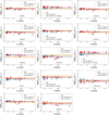Fig. E.1 log Lacc as a function of the wavelength for CTTS in the OB1, σOri, ϵCha and Corona Australis star forming regions. The orange line represents the log $L_{\text{acc\hspace{0.17em}}}^{XS}$ computed using the XS-fit method and its associated extinction value ($A_V^{XS}$). The blue dots show log $L_{\mathrm{a}\mathrm{c}\mathrm{c}}^{\mathrm{lines}}$ (Table A.1) calculated from the accretion tracers using the empirical relations from Alcalá et al. (2014), with fluxes dereddened using $A_V^{XS}$. Similarly, the red dots represent $L_{\text{acc\hspace{0.17em}}}^{line-diff}$, computed from the same accretion tracers but with fluxes dereddened using $A_V^{diff}$ (see Sect. 3.6 and Table 1). The blue and red dashed lines indicate the mean log Lacc values for the accretion tracers log Lacc,i in their respective colors.

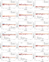Fig. E.2 log Lacc as a function of the wavelength for CTTS in the ηCha and Chamaeleon I star forming regions. Symbols are as in Fig. E.1.

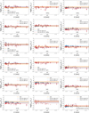Fig. E.3 log Lacc as a function of the wavelength for CTTS in the Taurus Auriga and Lupus star forming regions. Symbols are as in Fig. E.1.

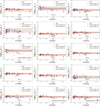Fig. E.4 log Lacc as a function of the wavelength for CTTS in the Lupus star forming region. Symbols are as in Fig. E.1.

Appendix F Plots for the Brackett lines discussed in the text

Figs. F.1 and F.2 shows the L_acc − L_line correlation for some lines of the Brackett series derived using the results of the XS- and HST-fit, respectively. Coefficients of empirical relations are listed in Table F.1 only for lines detected in more than 10 sources.

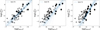Fig. F.1 log Lacc − log Lline and best fit for the Brackett series, using $A_V^{XS}$ to deredden the fluxes.

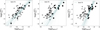Fig. F.2 log Lacc − log Lline and best fit for the Brackett series, using $A_V^{HST}$ to deredden the fluxes.

All Tables

All Figures

Fig. 1 X-shooter spectrum of the CTTS VW Cha. The UVB, VIS and NIR spectra are plotted in blue, yellow, and red, respectively. The UV-excess (blue region), tracing the accretion activity, and the NIR-excess (red region), tracing the presence of an active disk, are highlighted. The black curved dashed line corresponds to a stylized stellar photosphere + continuum veiling. All the accretion tracers for which Alcalá et al. (2017) provided empirical relations are shown in different colors, but not all the lines are labelled in the figure because of limited space. Also Br13, Br11, and Br10 lines are shown. Note: the spectrum starting wavelength was artificially set at ~320 nm for plotting purposes, while the actual UV-cut of X-shooter is at ~300 nm.

In the text

	Fig. 2 Histograms of accretion luminosity (top) and stellar mass (bottom) for the Lupus sample from (Alcalá et al. 2017, blue), PENELLOPE sample (orange), and ODYSSEUS sample (pink). All histograms are based on the same bin width: 0.5 dex for log Lacc and 0.2 M⊙ for the stellar mass.
In the text

Fig. 3 Comparison of Lacc computed using the HST modeling with that from the XS-fit. Left: log $L_{\text{acc\hspace{0.17em}}}^{HST}$ vs. log $L_{\text{acc\hspace{0.17em}}}^{XS}$, the pink line show the best fit, which is linear within the error with its dispersion. Right: differential analysis, the pink region corresponds to the standard deviation of log $L_{\mathrm{a}\mathrm{c}\mathrm{c}}^{HST}$ − log $L_{\mathrm{a}\mathrm{c}\mathrm{c}}^{XS}$, computed as the quadrature sum of the individual errors.

In the text

	Fig. 4 Left: comparison of AV computed using the HST- and XS- modelling. Right: comparison of AV using the HST-fit and the difference method of Sect. 3.6). The dashed line shows the one-to-one relation. The σ in both cases is 0.4.
In the text

Fig. 5 Comparison of the slopes (top) and intercepts (bottom) of the log Lacc − log Llines empirical relations derived in this work with those from Alcalá et al. (2017). The colorbar indicates the corresponding wavelength of each accretion tracer, ranging from UVB (blue) to NIR (yellow). Dark and light gray regions represent agreement within 1σ and 2σ, respectively. Accretion tracers not in agreement within 1σ (2σ) within the error are plotted as squares (triangles).

In the text

Fig. 6 $\log (<L_{\mathrm{a}\mathrm{c}\mathrm{c}}^{lines}>)$ vs. log $L_{\text{acc\hspace{0.17em}}}^{\text{modeling}}$. Colors of the points represent different star-forming regions as described in the legend. The blue line corresponds to our best fit. The dashed black line shows the linear trend as a reference. Left: log < Lacc >lines is computed as the average from the Lacc’s from many lines and using empirical relations by Alcalá et al. (2017) and log $L_{\text{acc\hspace{0.17em}}}^{XS}$ is obtained using the XS-fit method. Right: log < Lacc >lines is computed as the average from the Lacc’s from many lines and using empirical relations obtained in this work and log $L_{\text{acc\hspace{0.17em}}}^{HST}$ is obtained using the HST-fit method.

In the text

Fig. 7 Left panels: fraction of the total luminosity in lines relative to the accretion luminosity, i.e. the continuum excess luminosity. The light blue region corresponds to the range of values found in Alcalá et al. (2014). Right panels: total luminosity from the lines as a function of the log Lacc as indicated in the labels. The blue line in each panel corresponds to our best fit, while the light-blue lines give an indication of the spread of the fit (see Sect. 3.4). The dashed gray lines show the one-to-one relation. Red circled black dots correspond to sources where the Brγ line is detected.

In the text

	Fig. 8 Top panels: comparison between $A_V^{XS}$ and the extinction drawn from the coefficient method without weights (left), the method weighting for the error (central), and the difference method. Lower panels: comparison between average Lacc computed with the three methods and $L_{\mathrm{a}\mathrm{c}\mathrm{c}}^{XS}$. The blue line corresponds to the best fit.
In the text

Fig. 9 log Lacc as a function of the wavelength for two PENELLOPE CTTSs. Filled (empty) circles are log Lacc values computed using empirical relations, corresponding to suggested (non suggested) lines by Alcalá et al. (2014), while triangles represent upper limits. In red and blue results obtained by dereddening the flux with $A_V^{diff}$ and $A_V^{XS}$ are shown, respectively. Horizontal red and blue dashed lines and regions correspond to mean value and standard deviation of Lacc using $A_V^{diff}$ and $A_V^{XS}$, respectively. The orange solid line shows $L_{\text{acc\hspace{0.17em}}}^{XS}$ with its error bar (orange horizontal region). Top: plot for the multiple system VW Cha, where the extinction and accretion luminosity estimated with the difference method and the XS-fit are in agreement and the log Lacc distributions are flat. Bottom: SO1152 young star, where $A_V^{diff}$ and $A_V^{XS}$ differ by 1.5 mag and the distribution of log Lacc obtained by dereddening the fluxes with $A_V^{diff}$ is flatter than the one obtained using $A_V^{XS}$. The latter increases with the wavelength.

In the text

	Fig. 10 Slopes of empirical relations of Alcalá et al. (2017) sample (filled circles), this work (filled stars), and from the literature (Salyk et al. 2013; Rigliaco et al. 2015; Komarova & Fischer 2020; Rogers et al. 2024; Tofflemire et al. 2025, filled squares), as a function of the wavelength. Error bars are smaller than the symbols when not visible.
In the text

	Fig. B.1 Comparison of Lacc as in Fig. 3. The colored bar shows the difference in time between XS and HST observations for each target.
In the text

	Fig. D.1 log Lacc − log Lline and best fit for the Balmer series, the Paschen series and the Brγ line. The blue and orange lines show out best fit and the best fit from Alcalá et al. (2014), respectively. The wavelength in nanometers of each line is shown on the x-axis. Triangles are upper limits.
In the text

	Fig. D.2 log Lacc − log Lline and best fit for the helium, calcium, sodium, and oxygen accretion tracers. The blue and orange lines show our best fit and the best fit from Alcalá et al. (2017), respectively. The wavelength in nanometers of each line is shown on the x-axis. Triangles are upper limits.
In the text

Fig. E.1 log Lacc as a function of the wavelength for CTTS in the OB1, σOri, ϵCha and Corona Australis star forming regions. The orange line represents the log $L_{\text{acc\hspace{0.17em}}}^{XS}$ computed using the XS-fit method and its associated extinction value ($A_V^{XS}$). The blue dots show log $L_{\mathrm{a}\mathrm{c}\mathrm{c}}^{\mathrm{lines}}$ (Table A.1) calculated from the accretion tracers using the empirical relations from Alcalá et al. (2014), with fluxes dereddened using $A_V^{XS}$. Similarly, the red dots represent $L_{\text{acc\hspace{0.17em}}}^{line-diff}$, computed from the same accretion tracers but with fluxes dereddened using $A_V^{diff}$ (see Sect. 3.6 and Table 1). The blue and red dashed lines indicate the mean log Lacc values for the accretion tracers log Lacc,i in their respective colors.

In the text

	Fig. E.2 log Lacc as a function of the wavelength for CTTS in the ηCha and Chamaeleon I star forming regions. Symbols are as in Fig. E.1.
In the text

	Fig. E.3 log Lacc as a function of the wavelength for CTTS in the Taurus Auriga and Lupus star forming regions. Symbols are as in Fig. E.1.
In the text

	Fig. E.4 log Lacc as a function of the wavelength for CTTS in the Lupus star forming region. Symbols are as in Fig. E.1.
In the text

	Fig. F.1 log Lacc − log Lline and best fit for the Brackett series, using $A_V^{XS}$ to deredden the fluxes.
In the text

	Fig. F.2 log Lacc − log Lline and best fit for the Brackett series, using $A_V^{HST}$ to deredden the fluxes.
In the text

References

- Alcalá, J. M., Natta, A., Manara, C. F., et al. 2014, A&A, 561, A2 [NASA ADS] [CrossRef] [EDP Sciences] [Google Scholar]
- Alcalá, J. M., Manara, C. F., Natta, A., et al. 2017, A&A, 600, A20 [NASA ADS] [CrossRef] [EDP Sciences] [Google Scholar]
- Alcalá, J. M., Manara, C. F., France, K., et al. 2019, A&A, 629, A108 [NASA ADS] [CrossRef] [EDP Sciences] [Google Scholar]
- Almendros-Abad, V., Manara, C. F., Testi, L., et al. 2024, A&A, 685, A118 [NASA ADS] [CrossRef] [EDP Sciences] [Google Scholar]
- André, P. 1995, Ap&SS, 224, 29 [CrossRef] [Google Scholar]
- Antoniucci, S., Nisini, B., Giannini, T., & Lorenzetti, D. 2008, A&A, 479, 503 [NASA ADS] [CrossRef] [EDP Sciences] [Google Scholar]
- Aoyama, Y., Marleau, G.-D., Ikoma, M., & Mordasini, C. 2021, ApJ, 917, L30 [CrossRef] [Google Scholar]
- Armeni, A., Stelzer, B., Claes, R. A. B., et al. 2023, A&A, 679, A14 [NASA ADS] [CrossRef] [EDP Sciences] [Google Scholar]
- Armeni, A., Stelzer, B., Frasca, A., et al. 2024, A&A, 690, A225 [NASA ADS] [CrossRef] [EDP Sciences] [Google Scholar]
- Audard, M., Ábrahám, P., Dunham, M. M., et al. 2014, in Protostars and Planets VI, eds. H. Beuther, R. S. Klessen, C. P. Dullemond, & T. Henning (Tucson: University of Arizona Press), 387 [Google Scholar]
- Baraffe, I., Homeier, D., Allard, F., & Chabrier, G. 2015, A&A, 577, A42 [NASA ADS] [CrossRef] [EDP Sciences] [Google Scholar]
- Bertout, C., Basri, G., & Bouvier, J. 1988, ApJ, 330, 350 [Google Scholar]
- Bouvier, J., & Bertout, C. 1986, in Cool Stars, Stellar Systems and the Sun, eds. M. Zeilik & D. M. Gibson (Berlin: Springer-Verlag), 254, 132 [Google Scholar]
- Bouvier, J., Chelli, A., Allain, S., et al. 1999, A&A, 349, 619 [NASA ADS] [Google Scholar]
- Bouvier, J., Grankin, K., Ellerbroek, L. E., Bouy, H., & Barrado, D. 2013, A&A, 557, A77 [NASA ADS] [CrossRef] [EDP Sciences] [Google Scholar]
- Bowler, B. P., Zhou, Y., Biddle, L. I., et al. 2025, AJ, 169, 258 [Google Scholar]
- Calvet, N., & Gullbring, E. 1998, ApJ, 509, 802 [Google Scholar]
- Cardelli, J. A., Clayton, G. C., & Mathis, J. S. 1989, ApJ, 345, 245 [Google Scholar]
- Cauley, P. W., Shkolnik, E. L., Llama, J., & Lanza, A. F. 2019, Nat. Astron., 3, 1128 [NASA ADS] [CrossRef] [Google Scholar]
- Chabrier, G., Johansen, A., Janson, M., & Rafikov, R. 2014, in Protostars and Planets VI, eds. H. Beuther, R. S. Klessen, C. P. Dullemond, & T. Henning (Tucson: University of Arizona Press), 619 [Google Scholar]
- Claes, R. A. B., Campbell-White, J., Manara, C. F., et al. 2024, A&A, 690, A122 [NASA ADS] [CrossRef] [EDP Sciences] [Google Scholar]
- Cody, A. M., Hillenbrand, L. A., & Rebull, L. M. 2022, AJ, 163, 212 [NASA ADS] [CrossRef] [Google Scholar]
- Connerney, J. E. P., Kotsiaros, S., Oliversen, R. J., et al. 2018, Geophys. Res. Lett., 45, 2590 [Google Scholar]
- Costigan, G., Vink, J. S., Scholz, A., Ray, T., & Testi, L. 2014, MNRAS, 440, 3444 [NASA ADS] [CrossRef] [Google Scholar]
- Cruz-Sáenz de Miera, F., Kóspál, Á., Abrahám, P., et al. 2023, A&A, 678, A88 [NASA ADS] [CrossRef] [EDP Sciences] [Google Scholar]
- Delabrosse, V., Dougados, C., Cabrit, S., et al. 2024, A&A, 688, A173 [NASA ADS] [CrossRef] [EDP Sciences] [Google Scholar]
- Edwards, S., Fischer, W., Hillenbrand, L., & Kwan, J. 2006, ApJ, 646, 319 [Google Scholar]
- Enoch, M. L., Evans, Neal J., I., Sargent, A. I., & Glenn, J. 2009, ApJ, 692, 973 [NASA ADS] [CrossRef] [Google Scholar]
- Espaillat, C. C., Herczeg, G. J., Thanathibodee, T., et al. 2022, AJ, 163, 114 [NASA ADS] [CrossRef] [Google Scholar]
- Fiorellino, E., Manara, C. F., Nisini, B., et al. 2021, A&A, 650, A43 [NASA ADS] [CrossRef] [EDP Sciences] [Google Scholar]
- Fiorellino, E., Park, S., Kóspál, Á., & Ábrahám, P. 2022a, ApJ, 928, 81 [Google Scholar]
- Fiorellino, E., Zsidi, G., Kóspál, À., et al. 2022b, ApJ, 938, 93 [NASA ADS] [CrossRef] [Google Scholar]
- Fiorellino, E., Tychoniec, Ł., Cruz-Sáenz de Miera, F., et al. 2023, ApJ, 944, 135 [NASA ADS] [CrossRef] [Google Scholar]
- Fiorellino, E., Ábrahám, P., Kóspál, Á., et al. 2024, A&A, 686, A160 [NASA ADS] [CrossRef] [EDP Sciences] [Google Scholar]
- Flores, C., Connelley, M. S., Reipurth, B., Boogert, A., & Doppmann, G. 2024, ApJ, 972, 149 [NASA ADS] [CrossRef] [Google Scholar]
- Gaia Collaboration (Brown, A. G. A., et al.) 2021, A&A, 650, C3 [EDP Sciences] [Google Scholar]
- Giannini, T., Schisano, E., Nisini, B., et al. 2024, ApJ, 967, 41 [Google Scholar]
- Greene, T. P., Wilking, B. A., Andre, P., Young, E. T., & Lada, C. J. 1994, ApJ, 434, 614 [NASA ADS] [CrossRef] [Google Scholar]
- Gullbring, E., Hartmann, L., Briceño, C., & Calvet, N. 1998, ApJ, 492, 323 [Google Scholar]
- Haffert, S. Y., Bohn, A. J., de Boer, J., et al. 2019, Nat. Astron., 3, 749 [Google Scholar]
- Halstead Willett, L., Ninan, J. P., Mahadevan, S., et al. 2025, arXiv e-prints [arXiv:2501.10500] [Google Scholar]
- Harsono, D., Bjerkeli, P., Ramsey, J. P., et al. 2023, ApJ, 951, L32 [NASA ADS] [CrossRef] [Google Scholar]
- Hartmann, L., Calvet, N., Gullbring, E., & D’Alessio, P. 1998, ApJ, 495, 385 [Google Scholar]
- Hartmann, L., Herczeg, G., & Calvet, N. 2016, ARA&A, 54, 135 [Google Scholar]
- Hashimoto, J., & Aoyama, Y. 2025, AJ, 169, 93 [Google Scholar]
- Herczeg, G. J., & Hillenbrand, L. A. 2008, ApJ, 681, 594 [Google Scholar]
- Hodapp, K. W., Denneau, L., Tucker, M., et al. 2020, AJ, 160, 164 [NASA ADS] [CrossRef] [Google Scholar]
- Ingleby, L., Calvet, N., Herczeg, G., et al. 2013, ApJ, 767, 112 [Google Scholar]
- Kausch, W., Noll, S., Smette, A., et al. 2015, A&A, 576, A78 [NASA ADS] [CrossRef] [EDP Sciences] [Google Scholar]
- Kelly, B. C. 2007, ApJ, 665, 1489 [Google Scholar]
- Kenyon, S. J., & Hartmann, L. 1995, ApJS, 101, 117 [Google Scholar]
- Komarova, O., & Fischer, W. J. 2020, Res. Notes Am. Astron. Soc., 4, 6 [Google Scholar]
- Lodato, G., Scardoni, C. E., Manara, C. F., & Testi, L. 2017, MNRAS, 472, 4700 [NASA ADS] [CrossRef] [Google Scholar]
- Luhman, K. L., Stauffer, J. R., Muench, A. A., et al. 2003, ApJ, 593, 1093 [Google Scholar]
- Lynden-Bell, D., & Pringle, J. E. 1974, MNRAS, 168, 603 [Google Scholar]
- Manara, C. F., Beccari, G., Da Rio, N., et al. 2013a, A&A, 558, A114 [NASA ADS] [CrossRef] [EDP Sciences] [Google Scholar]
- Manara, C. F., Testi, L., Rigliaco, E., et al. 2013b, A&A, 551, A107 [NASA ADS] [CrossRef] [EDP Sciences] [Google Scholar]
- Manara, C. F., Testi, L., Herczeg, G. J., et al. 2017, A&A, 604, A127 [NASA ADS] [CrossRef] [EDP Sciences] [Google Scholar]
- Manara, C. F., Frasca, A., Venuti, L., et al. 2021, A&A, 650, A196 [NASA ADS] [CrossRef] [EDP Sciences] [Google Scholar]
- Manara, C. F., Ansdell, M., Rosotti, G. P., et al. 2023, ASP Conf. Ser., 534, 539 [NASA ADS] [Google Scholar]
- Maucó, K., Manara, C. F., Ansdell, M., et al. 2023, A&A, 679, A82 [NASA ADS] [CrossRef] [EDP Sciences] [Google Scholar]
- Maucó, K., Manara, C. F., Bayo, A., et al. 2025, A&A, 693, A87 [NASA ADS] [CrossRef] [EDP Sciences] [Google Scholar]
- Mendigutía, I., Oudmaijer, R. D., Rigliaco, E., et al. 2015, MNRAS, 452, 2837 [Google Scholar]
- Modigliani, A., Goldoni, P., Royer, F., et al. 2010, SPIE Conf. Ser., 7737, 773728 [Google Scholar]
- Mohanty, S., Basri, G., & Jayawardhana, R. 2005, Astron. Nachr., 326, 891 [Google Scholar]
- Mulders, G. D., Pascucci, I., Manara, C. F., et al. 2017, ApJ, 847, 31 [NASA ADS] [CrossRef] [Google Scholar]
- Muzerolle, J., Hartmann, L., & Calvet, N. 1998, AJ, 116, 2965 [NASA ADS] [CrossRef] [Google Scholar]
- Pittman, C. V., Espaillat, C. C., Robinson, C. E., et al. 2022, AJ, 164, 201 [NASA ADS] [CrossRef] [Google Scholar]
- Pittman, C. V., Espaillat, C. C., Robinson, C. E., et al. 2025, arXiv e-prints [arXiv:2507.01162] [Google Scholar]
- Plunkett, C., Follette, K. B., Marleau, G.-D., & Nielsen, E. L. 2025, AJ, 169, 262 [Google Scholar]
- Pouilly, K., Hahlin, A., Kochukhov, O., Morin, J., & Kóspál, Á. 2024, MNRAS, 528, 6786 [NASA ADS] [CrossRef] [Google Scholar]
- Reiners, A., & Basri, G. 2007, ApJ, 656, 1121 [NASA ADS] [CrossRef] [Google Scholar]
- Rigliaco, E., Natta, A., Randich, S., & Sacco, G. 2009, A&A, 495, L13 [NASA ADS] [CrossRef] [EDP Sciences] [Google Scholar]
- Rigliaco, E., Natta, A., Testi, L., et al. 2012, A&A, 548, A56 [NASA ADS] [CrossRef] [EDP Sciences] [Google Scholar]
- Rigliaco, E., Pascucci, I., Duchene, G., et al. 2015, ApJ, 801, 31 [Google Scholar]
- Ringqvist, S. C., Viswanath, G., Aoyama, Y., et al. 2023, A&A, 669, L12 [NASA ADS] [CrossRef] [EDP Sciences] [Google Scholar]
- Rogers, C., de Marchi, G., & Brandl, B. 2024, A&A, 684, L8 [NASA ADS] [CrossRef] [EDP Sciences] [Google Scholar]
- Roman-Duval, J., Proffitt, C. R., Taylor, J. M., et al. 2020, Res. Notes Am. Astron. Soc., 4, 205 [Google Scholar]
- Roman-Duval, J., Fischer, W. J., Fullerton, A. W., et al. 2025, ApJ, 985, 109 [Google Scholar]
- Rugel, M., Fedele, D., & Herczeg, G. 2018, A&A, 609, A70 [NASA ADS] [CrossRef] [EDP Sciences] [Google Scholar]
- Salyk, C., Herczeg, G. J., Brown, J. M., et al. 2013, ApJ, 769, 21 [CrossRef] [Google Scholar]
- Schneider, P. C., Günther, H. M., & France, K. 2020, Galaxies, 8, 27 [NASA ADS] [CrossRef] [Google Scholar]
- Sicilia-Aguilar, A., Henning, T., & Hartmann, L. W. 2010, ApJ, 710, 597 [Google Scholar]
- Siess, L., Dufour, E., & Forestini, M. 2000, A&A, 358, 593 [Google Scholar]
- Singh, K., Ninan, J. P., Romanova, M. M., et al. 2024, ApJ, 968, 88 [NASA ADS] [CrossRef] [Google Scholar]
- Siwak, M., Hillenbrand, L. A., Kóspál, Á., et al. 2023, MNRAS, 524, 5548 [NASA ADS] [CrossRef] [Google Scholar]
- Smette, A., Sana, H., Noll, S., et al. 2015, A&A, 576, A77 [NASA ADS] [CrossRef] [EDP Sciences] [Google Scholar]
- Somigliana, A., Testi, L., Rosotti, G., et al. 2023, ApJ, 954, L13 [NASA ADS] [CrossRef] [Google Scholar]
- Tabone, B., Rosotti, G. P., Lodato, G., et al. 2022, MNRAS, 512, L74 [NASA ADS] [CrossRef] [Google Scholar]
- Tofflemire, B. M., Manara, C. F., Banzatti, A., et al. 2025, arXiv e-prints [arXiv:2504.08029] [Google Scholar]
- Turner, N. J., Lee, M. H., & Sano, T. 2014, ApJ, 783, 14 [NASA ADS] [CrossRef] [Google Scholar]
- Tychoniec, Ł., van Gelder, M. L., van Dishoeck, E. F., et al. 2024, A&A, 687, A36 [NASA ADS] [CrossRef] [EDP Sciences] [Google Scholar]
- Valenti, J. A., Basri, G., & Johns, C. M. 1993, AJ, 106, 2024 [NASA ADS] [CrossRef] [Google Scholar]
- Viswanath, G., Ringqvist, S. C., Demars, D., et al. 2024, A&A, 691, A64 [NASA ADS] [CrossRef] [EDP Sciences] [Google Scholar]
- Vorobyov, E., & Elbakyan, V. 2020, in Stars and their Variability Observed from Space, eds. C. Neiner, W. W. Weiss, D. Baade, R. E. Griffin, C. C. Lovekin, & A. F. J. Moffat (Vienna: University of Vienna), 363 [Google Scholar]
- Wendeborn, J., Espaillat, C. C., Lopez, S., et al. 2024a, ApJ, 970, 118 [Google Scholar]
- Wendeborn, J., Espaillat, C. C., Thanathibodee, T., et al. 2024b, ApJ, 972, 100 [NASA ADS] [CrossRef] [Google Scholar]
- Whelan, E. T., Riaz, B., & Rouzé, B. 2018, A&A, 610, L19 [NASA ADS] [CrossRef] [EDP Sciences] [Google Scholar]
- Zhou, Y., Bowler, B. P., Wagner, K. R., et al. 2021, AJ, 161, 244 [NASA ADS] [CrossRef] [Google Scholar]
IRAF is distributed by the National Optical Astronomy Observatories, which are operated by the Association of Universities for Research in Astronomy, Inc., under the cooperative agreement with the National Science Foundation. NOAO stopped supporting IRAF, see https://iraf-community.github.io