| Issue |
A&A
Volume 704, December 2025
|
|
|---|---|---|
| Article Number | A75 | |
| Number of page(s) | 12 | |
| Section | The Sun and the Heliosphere | |
| DOI | https://doi.org/10.1051/0004-6361/202556857 | |
| Published online | 28 November 2025 | |
An automated, self-calibration-based pipeline for high-fidelity solar imaging with LOFAR: SIMPL
1
National Centre for Radio Astrophysics, Tata Institute of Fundamental Research, S. P. Pune University Campus, Pune 411007, India
2
ASTRON – The Netherlands Institute for Radio Astronomy, Oude Hoogeveensedijk 4, 7991 PD Dwingeloo, The Netherlands
3
NASA Jack Eddy Fellow, University Corporation for Atmospheric Research, 3090 Center Green Dr, Boulder, CO 80301, USA
4
The Johns Hopkins University Applied Physics Laboratory, 11001 Johns Hopkins Rd, Laurel 20723, USA
⋆ Corresponding author: This email address is being protected from spambots. You need JavaScript enabled to view it.
Received:
14
August
2025
Accepted:
22
September
2025
Abstract
Context. The LOw Frequency ARray (LOFAR) is capable of imaging spectroscopy of the Sun in the 10–240 MHz frequency range, with high spectral, temporal, and spatial resolution. However, the complex and rapidly varying nature of solar radio emission – spanning several orders of magnitude in brightness and further exacerbated by the strong ionospheric phase distortions during daytime observations, poses major challenges for calibration, imaging, and automation.
Aims. We aim to develop a fully automated, high-fidelity imaging pipeline optimised for LOFAR solar observations, capable of handling the intrinsic variability of solar emission and producing science-ready images with minimal human intervention.
Methods. We have built the Solar Imaging Pipeline for LOFAR (SIMPL), which integrates excision of radio-frequency interference (RFI) for the solar-specific scenarios, calibration strategies, and self-calibration. At present, SIMPL processes data from the LOFAR core stations and produces total-intensity solar images, with ongoing developments aimed at enabling full polarimetric imaging and incorporating increasingly distant antennas. The pipeline is designed to enable scalable and uniform processing of large archival datasets.
Results. In terms of performance, SIMPL achieves more than an order of magnitude improvement in imaging dynamic range compared with previous efforts and reliably produces high-quality spectroscopic snapshot images. It has been tested across a wide range of solar conditions. It is currently being employed to process a decade of LOFAR solar observations, providing science-ready Flexible Image Transport System (FITS) images for the community and enabling both comprehensive and novel studies of solar radio phenomena, ranging from quiet Sun emission and faint non-thermal features to active regions and their associated dynamic events, such as transient bursts.
Key words: techniques: interferometric / Sun: corona / Sun: radio radiation
© The Authors 2025
 Open Access article, published by EDP Sciences, under the terms of the Creative Commons Attribution License (https://creativecommons.org/licenses/by/4.0), which permits unrestricted use, distribution, and reproduction in any medium, provided the original work is properly cited.
This article is published in open access under the Subscribe to Open model. This email address is being protected from spambots. You need JavaScript enabled to view it. to support open access publication.
1. Introduction
Imaging the radio Sun with high fidelity is an intrinsically challenging endeavour. The solar corona is a complex, dynamic, and magnetised plasma environment that produces radio emissions across a broad range of angular scales and emission mechanisms. These emission mechanisms give rise to brightness temperatures (TB) that can vary by many orders of magnitude over small time and frequency intervals (e.g. Kansabanik 2022), spanning a vast range of angular scales. At metre wavelengths, for instance, thermal bremsstrahlung from the quiescent Sun typically shows TB ∼ 106 K (e.g. Mercier & Chambe 2015; Oberoi et al. 2017; Vocks et al. 2018). In stark contrast, coherent emission processes, often triggered by flare-accelerated electron beams, can generate extreme type III bursts with TB soaring beyond 1011 K (e.g. Melrose 1989; Saint-Hilaire et al. 2013). Capturing these emissions, which cover an immense dynamic range, is further complicated by their rapid spectro-temporal evolution on sub-second timescales, with fractional bandwidths δν/ν0 ≪ 1 (e.g. Ratcliffe et al. 2014; Clarkson et al. 2023). Consequently, achieving a comprehensive understanding of coronal dynamics necessitates high-fidelity spectroscopic snapshot imaging capable of ‘freezing’ these rapid changes in both time and frequency.
The challenge is exacerbated by the frequent superposition of diverse morphological structures, ranging from intensely bright, compact bursts to faint, diffuse background emissions (e.g. Kansabanik 2022; Dey et al. 2025). Furthermore, the Sun’s extreme flux density compared to typical calibrator sources introduces significant complexities in achieving robust calibration (e.g. Mondal et al. 2019; Kansabanik 2022; Kansabanik et al. 2022). Historically, these limitations, compounded by the capabilities of earlier instruments, meant that radio imaging studies of dynamic solar emission were often restricted to the brightest emission sources at a few discrete frequencies (see numerous examples in McLean & Labrum 1985; Pick & Vilmer 2008; Nindos 2020). Investigations of the much fainter quiet Sun, in contrast, usually necessitated integration times spanning many hours (e.g. Mercier & Chambe 2009; Zhang et al. 2022a). Even with an advanced instrument such as the LOw Frequency ARray (LOFAR; van Haarlem et al. 2013), imaging studies often focused on the brightest events or relied on long integrations.
The advent of new-generation metric radio interferometers, including LOFAR (operating in the 10−90 MHz and 110−240 MHz bands), the Long Wavelength Array at the Owens Valley Radio Observatory (OVRO-LWA; Anderson et al. 2018; Hallinan et al. 2023; 12−85 MHz), and the Murchison Widefield Array (MWA; Tingay et al. 2013; Wayth et al. 2018; 80−300 MHz), driven by enormous advances in digital signal processing and computational power, represents a significant leap in instrumental capabilities. These instruments are exceptionally well-suited for solar imaging with high temporal and spectral resolution at low radio frequencies and are already yielding a wealth of interesting scientific results (e.g. Morosan et al. 2015, 2019; Suresh et al. 2017; Zucca et al. 2018, 2025; McCauley et al. 2019; Mohan et al. 2019; Mondal et al. 2020a,b, 2023; Chhabra et al. 2021; Sharma et al. 2022; Bhunia et al. 2023; Oberoi et al. 2023; Kansabanik et al. 2024; Dey et al. 2025). Dynamic imaging spectroscopy with LOFAR, for example, has begun to reveal previously unseen burst morphologies, such as spatially resolved radio signatures of electron beams in coronal shocks (Zhang et al. 2024) and images of intricate fine structures seen in dynamic spectra associated with type III bursts (Dabrowski et al. 2025). With more than a decade of such LOFAR observations – more than 2200 hours spanning solar cycles 24–25 now archived – the sheer volume of these information-rich data makes manual analysis impractical. A fully automated and robust pipeline is therefore essential for the uniform processing of this extensive dataset and for enabling crucial long-term statistical studies.
In this work, we present the Solar IMaging Pipeline for LOFAR (SIMPL) – a fully automated and robust calibration and imaging pipeline specifically designed for solar radio observations with LOFAR. This pipeline integrates solar-specific radio-frequency interference (RFI) mitigation techniques, tailored calibration strategies, and a self-calibration framework optimised for the Sun’s complex and dynamic emission. Together, these enable the generation of high-fidelity spectroscopic snapshot images, significantly improving the dynamic range and fidelity of LOFAR solar radio images. The pipeline is currently being employed to systematically process over a decade of solar interferometric observations, to provide science-ready FITS files that can be accessed on demand by the broader solar physics community.
The paper is organised as follows. Section 2 provides a brief overview of the LOFAR instrument and its solar observing modes. Section 3 outlines the challenges in calibration and imaging of solar observations at low radio frequencies. In Section 4, we review existing solar imaging pipelines for LOFAR and their limitations. Section 5 presents the algorithmic design of SIMPL. Results demonstrating the pipeline’s performance are shown in Section 6. Section 7 describes the integration of the pipeline into the existing LOFAR processing framework, and finally, Section 8 outlines the directions for future development, followed by conclusions in Section 9.
2. LOFAR
The LOw Frequency ARray (LOFAR) is a state-of-the-art interferometer operating across the 10−240 MHz frequency range. It comprises 38 stations in the Netherlands and 14 international stations across Europe. Of the 38 Dutch stations, 24 are located within ∼2 km at Exloo. This cluster of stations is referred to as the ‘core’. Each station hosts two antenna fields – the low-band antennas (LBAs; 10−90 MHz) and the high-band antennas (HBAs; 110−240 MHz) – each providing data in both orthogonal linear polarisations, with signals digitised and beamformed locally before being streamed to the central correlator in Groningen. In the interferometric mode1, LOFAR provides the following specifications:
-
The instantaneous bandwidth is split into 512 sub-bands via a polyphase filter.
-
Up to 244 sub-bands (≈48 MHz total bandwidth) can be selected and sent to the correlator in 16-bit mode (or 488 sub-bands in 8-bit mode).
-
Each sub-band spans 195.3 kHz or 156.2 kHz (for the 200 MHz or 160 MHz clock, respectively), which can be further channelised (e.g. into 64 channels yielding ∼3 kHz resolution).
-
The minimum integration time is ∼0.16 seconds.
The array allows concurrent observations of multiple sky regions (Broekema et al. 2018) using simultaneous station beams. For solar observations, a strong calibrator source (e.g. Cassiopeia A or Taurus A) is usually observed simultaneously using an independent LOFAR station beam. This approach avoids interrupting the solar observation for separate calibrator scans, as is conventionally done, and instead derives complex antenna gains from the simultaneously observed calibrator that are then applied to the solar beam. Considering only the core stations, 276 baselines are available instantaneously for the LBA and 1128 for the HBA. Instantaneous uv-coverage for a single spectral slice for LOFAR is shown in Figure 1: LBA (a) and HBA (b). Thus, LOFAR provides high time and spectral resolution, along with reasonable instantaneous uv-coverage, giving it the spectroscopic snapshot imaging capability necessary for studying narrowband and transient solar emissions.
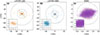 |
Fig. 1. Instantaneous uv-coverage comparison between the LOw Frequency ARray (LOFAR) and the Murchison Widefield Array (MWA). Projected baseline distributions are shown for (a) LOFAR-LBA, (b) LOFAR-HBA, and (c) the MWA Phase-II configuration. Both LOFAR-LBA and HBA exhibit densely clustered cores, providing high sensitivity to large-scale solar structures, complemented by longer remote baselines that enable higher spatial resolution. In contrast, the MWA provides a significantly denser and more uniformly distributed uv-coverage within a compact footprint, facilitating high-fidelity snapshot imaging at moderate resolution (a few arcminutes). Insets in each panel zoom into the central ±2 km region (marked by red squares) to highlight baseline distributions within the core. The dashed black circles indicate radii of 2.5, 5, 10, 20, and 50 km. The number of independent baselines from core antennas is 276 for LOFAR-LBA and 1128 for LOFAR-HBA. For panel c, representing the MWA phase-II configuration, there are 8128 instantaneous baselines within 5 km. |
3. Calibration challenges
The dynamic nature and extremely high flux densities of solar radio emission, described in Section 1, present substantial challenges for its calibration. Strong solar signals, including during quiet times, can contaminate calibrator observations, even when the calibrator is located several degrees away from the Sun. This issue is especially pronounced for wide field of view (FoV) aperture array instruments such as LOFAR. Figure 2 illustrates this problem: the upper panel shows dynamic spectra of the Sun, while the lower panel shows dynamic spectra of the simultaneously observed calibrator source, Cassiopeia A, located 11.4° away using a separate station beam. Signatures of essentially all of the narrow-band, short-lived solar emissions are evident in the dynamic spectra of the calibrator beam, demonstrating significant contamination of the calibrator beam by the solar signal. While contamination of the time-frequency-variable component of the solar emission is easily seen, contamination of the quiet-Sun emission is not visually evident from the dynamic spectrum.
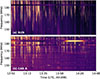 |
Fig. 2. Comparison of dynamic spectra (DS) from the Sun (a) and the calibrator Cassiopeia A (b), observed simultaneously with two separate LOFAR station beams. These DS were generated by averaging visibilities in the 150−500 λ range in the uv-plane to preferentially capture transient, compact structures while suppressing contributions from large-scale quiet Sun emission. Although Cassiopeia A was located 11.4° from the Sun during the observation, its DS shows features that strongly resemble those seen in the solar spectrum, indicating substantial solar contamination in the calibrator field. This highlights the difficulty of obtaining clean calibrator data during solar observing sessions, particularly with wide field of view (FoV) instruments such as LOFAR. |
Minimising this contamination by observing a calibrator much farther away introduces another major calibration difficulty at low radio frequencies, arising from ionospheric effects. The ionosphere introduces spatially and temporally varying phases across the sky, resulting in direction-dependent differential phase errors across the array. For narrow FoV interferometers, this is typically addressed by interleaving observations of the target source with frequent scans of a nearby phase calibrator. However, for solar observations, and with wide FoV instruments – where the Sun overwhelmingly dominates the sky emission – this approach becomes impractical. With LOFAR, an ‘A-team source’ is observed as a calibrator. These are extremely bright radio sources in the northern sky: Cassiopeia A, Cygnus A, Taurus A, and Virgo A. These observations capture the sum of direction-independent instrumental phases and direction-dependent ionospheric phases toward the calibrator. However, the derived phase solutions cannot correct for the (often large) differential phase towards the direction of the Sun, and this uncorrected phase difference can be large enough to significantly degrade image quality.
Figure 3 demonstrates this problem. The left panel shows an image of the calibrator (Virgo A) at a centre frequency of 113 MHz, made using a time and frequency integration of 53 s and 2 MHz, respectively. The image has a dynamic range exceeding 1250 and an rms of 0.08 Jy/beam. The flux density of Virgo A at 150 MHz is 1209 Jy (de Gasperin et al. 2020), comparable to the quiet-Sun flux density at this frequency. The middle panel shows the solar image obtained after applying calibration solutions derived from Virgo A at the same central frequency, with shorter spectral and temporal averaging spans of 1 MHz and 2 s, respectively. Accounting for the differences in spectral and temporal averaging, the expected rms noise level in the solar image – estimated from the measured rms of Virgo A – is 0.58 Jy/beam. The achieved map rms is 4.0 Jy/beam, resulting in an imaging dynamic range of ∼28. Beam gain corrections have not been applied to these images. The right panel shows the image for the same data and time-frequency integration made by SIMPL, which achieves a map rms of 0.5 Jy/beam, leading to an imaging dynamic range exceeding 550. The imaging strategy used by SIMPL is detailed in Section 5.
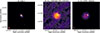 |
Fig. 3. Limitations of applying calibrator-based phase solutions across widely separated sky regions. Left panel: Image of Virgo A obtained using calibration solutions from the calibrator beam, demonstrating excellent fidelity and a dynamic range exceeding 1250 (rms: 0.08 Jy/beam). Middle panel: Solar image obtained by applying calibration solutions derived from the calibrator source Virgo A. The image suffers from significant phase errors, resulting in distorted morphology and a limited dynamic range of ∼28 (rms: 4.0 Jy/beam). Right panel: Solar image produced by the SIMPL pipeline using a self-calibration-based approach, yielding a markedly improved dynamic range of ∼550 (rms: 0.5 Jy/beam). Contours at each panel are drawn at −1%, 1%, 5%, 10%, 20%, 30%, 50%, 70%, and 90% of their respective peaks, with the negative contour shown as dashed yellow lines. The red ellipse in the bottom-left corner of each panel indicates the restoring beam. The comparison underscores the necessity of direction-dependent calibration for accurate high-fidelity solar imaging. |
4. Limitations of the existing LOFAR solar imaging pipelines
The calibration challenges described in Sections 1 and 3 have long posed significant hurdles for solar imaging, including challenges specific to LOFAR. Two notable efforts are commonly used for solar imaging studies with LOFAR: (i) the LOFAR Solar Imaging Pipeline developed by the Leibniz-Institut für Astrophysik Potsdam (AIP) group (Breitling et al. 2015) and (ii) LOFAR-Sun2 (Zhang et al. 2022a), a more recent and modular Python-based pipeline. Both pipelines build on standard tools from the LOFAR imaging ecosystem and rely on calibration solutions from a calibrator source, usually observed simultaneously with the Sun. Neither include solar-specific adaptations in their calibration strategies. Their processing workflow largely follows the procedures used in LOFAR’s standard imaging pipeline3 (van Haarlem et al. 2013), with minor modifications such as skipping automated flagging and source finding. In some cases, calibrator solutions have been manually derived during quiet solar periods when no active emission was evident.
Exclusively calibrator-based approaches often compromise solar imaging quality, particularly during elevated solar activity or significant ionospheric variability (Section 3). Although Breitling et al. (2015) mention optional phase-only self-calibration in their workflow, to the best of our knowledge, it has not been used in subsequent studies employing their pipeline (e.g. Dabrowski et al. 2025; Bröse et al. 2025). This underscores the need for dedicated solar calibration strategies tailored to the unique challenges of low-frequency solar radio interferometry.
5. Algorithm description
The SIMPL pipeline incorporates insights and experience gained from the development of dedicated solar imaging pipelines for the MWA (Mondal et al. 2019; Kansabanik et al. 2022, 2023), which introduced self-calibration strategies that are well suited to compact, centrally condensed arrays. The solar flux density usually drops substantially at longer baselines. Consequently, SIMPL is currently tailored to process solar interferometric data using only the LOFAR core stations and ignores the sparsely sampled remote baselines.
Unlike the MWA, which typically operated with 128 tiles in its phase I (Tingay et al. 2013) and II (Wayth et al. 2018) (and now up to 256 tiles in its phase III), producing 8128 simultaneous independent baselines within 5 km, LOFAR’s compact core provides significantly fewer baselines: 276 for the LBA and 1128 for the HBA within 2 km (Figure 1). The sparser uv-coverage provided by LOFAR, compared to MWA, inherently limits the achievable spectroscopic snapshot imaging dynamic range with LOFAR. Additionally, LOFAR typically observes calibrator sources simultaneously with the Sun (usually one of the A-team sources), while MWA schedules separate nighttime calibrator observations.
To provide an overview, in its current implementation, SIMPL first identifies the optimal time range within the calibrator observation to extract reliable calibration solutions. It then applies only the amplitude component of the antenna gain solutions to the solar data. The phase part of these solutions is derived entirely via self-calibration, using an iterative strategy with progressive baseline inclusion. The solar dataset is segmented into time-frequency chunks, and self-calibration is independently carried out and applied to each segment to account for time and frequency variations of complex gains, dominated primarily by variations in ionospheric phases. Finally, primary beam correction towards the direction of the Sun is applied, followed by the generation of spectroscopic snapshot images at user-defined time and frequency resolutions and intervals. A schematic overview of the processing pipeline is illustrated in Figure 4, with details provided in the following sub-sections.
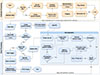 |
Fig. 4. Schematic overview of SIMPL. The flow is divided into three main sections: calibrator processing (orange), solar processing (light blue), and the self-calibration sub-module (darker blue). Calibrator processing identifies an optimal quiet time range for daytime observations, derives antenna gain solutions, and applies only the amplitude part of the gains to solar data. Solar processing operates on time–frequency chunks of the solar measurement set, invoking the self-calibration block to iteratively refine phase (and later amplitude) solutions. An optional higher dynamic range mode estimates differential self-calibration solutions per time and frequency slice. Final steps include primary beam correction and generation of spectroscopic snapshot images. Rounded rectangles denote processing steps, diamonds represent decision points, and dashed rounded rectangles indicate iterative self-calibration loops. |
5.1. Identifying optimal time for calibration from calibrator observation
The presence of solar emission features in the calibrator beam (Figure 2) demonstrates that simultaneous daytime calibrator observations can be severely contaminated by solar emission. The dynamic spectra were generated by averaging visibilities in the 150 − 500 λ range in the uv-plane to preferentially capture transient, compact structures while suppressing contributions from large-scale quiet-Sun emission.
To extract reliable calibration solutions from the daytime calibrator scan, it is essential to identify a time interval that is minimally affected by solar contamination. In SIMPL, we implement a composite score-based algorithm to automatically detect the quietest time window within the dynamic spectrum of the calibrator.
The algorithm is designed to identify a contiguous time segment with minimal statistical variation and minimal transient solar activity. A user-configurable sliding window (SW; default: 30 s) is moved across the time axis, using the available bandwidth, while computing the following statistical metrics:
-
Standard deviation (σ) and median absolute deviation (MAD)
-
Skewness and kurtosis: indicators of non-Gaussianity, with elevated values typically marking impulsive radio bursts
-
Shannon entropy: a measure of information content or randomness within the spectral profile, normalised to account for relative signal scaling.
Each metric is normalised independently using min-max scaling, where for a given metric, M, the normalised value is computed as
 (1)
(1)
and the composite score, z, is then calculated as
 (2)
(2)
The weights w1 to w5 are empirically determined from extensive testing across a large number of datasets and are set to 0.4, 0.4, 0.1, 0.1, and 0.1, respectively. Higher z values indicate stronger contamination. The resulting composite score time series is smoothed using a moving median filter with a window length SW/3 + 1.
A quiet-time threshold is then defined as the 25th percentile of the smoothed composite score distribution. All windows with z below this threshold are considered ‘quiet’, and the longest contiguous quiet segment is selected for calibration. Figure 5 illustrates this procedure, highlighting an example of the identified quiet interval within a calibrator dynamic spectrum severely contaminated by transient solar flux.
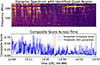 |
Fig. 5. Automated identification of a quiet calibration interval within contaminated calibrator data. The top panel shows the dynamic spectra of a calibrator observation (Cassiopeia A) contaminated by solar emission, with vertical dashed cyan lines marking the start and end of the automatically identified quiet interval. The bottom panel displays the smoothed composite score time series, derived from statistical measures of variability, non-Gaussianity, and entropy across sliding time windows. The horizontal green line marks the 25th percentile threshold used to define ‘quiet’ intervals. The selected segment (between red dashed lines, from 13:48:20 to 13:50:18 UTC) represents the longest continuous window below this threshold and is used for reliable calibration. |
5.2. Calibration using simultaneous calibrator observations
To mitigate solar contamination from calibrator observation, SIMPL first identifies a time interval during which the Sun is quiescent (see Section 5.1). This ensures that the calibration solutions are estimated from a time range of calibrator scan, which is devoid of transient solar contamination. Additionally, to avoid contamination from quiet-Sun emission originating from the extended solar disc, visibilities are restricted to an appropriate uv-range, typically greater than 100 λ.
The calibrator source is first identified and the corresponding model is imported using the Default Preprocessing Pipeline (DP3) (van Diepen et al. 2018) after multiplying with the LOFAR station beam. The raw calibrator dataset is initially flagged for RFI using the tfcrop algorithm within the flagdata task in the Common Astronomy Software Applications package (CASA; CASA Team 2022). Calibration is then performed in three iterations using the CASA task bandpass. After each iteration, automated flagging is performed using the rflag algorithm on the residual visibilities to remove low-level RFIs, followed by recalibration to obtain updated gain solutions.
Due to the direction dependence of ionospheric phases, the complex gain solutions derived from the direction of the calibrator are not the optimal solutions for the solar field. Figure 3 shows an example in which applying the gain solutions determined from the calibrator Virgo A yields a high-fidelity image when applied to it, with a dynamic range exceeding 1250 (left panel). The solar image obtained after applying the same calibration solutions suffers from significant phase errors, resulting in a dynamic range of only ∼28 (middle panel), illustrating that ionospheric conditions differ substantially across different parts of the sky.
To overcome this, SIMPL retains only the amplitude component of the calibrator-derived gain solutions for absolute flux scaling and disregards the phase solutions. The phases are instead derived via self-calibration directly on the solar data, as detailed in Section 5.3. This approach significantly improves image quality: for the same example, a dynamic range of ∼550 is achieved (Figure 3, right panel), along with better morphological fidelity.
5.3. Self-calibration
In standard radio interferometric calibration using calibrator sources, the sky model is well known. The complex direction–independent antenna gains, gp, are determined by minimising the following objective function:
 (3)
(3)
where Vpq are the observed visibilities and  are the model visibilities, with the summation over all baselines formed by antennas p and q. Here, * denotes the complex conjugate, so
  is the complex conjugate of the gain gq. Equation (3) presumes that the sky brightness distribution is accurately known a priori. When this assumption fails, both the gains and the sky model may be treated as free parameters, and Equation (3) generalises to
![Mathematical equation: $$ \begin{aligned} \Phi = \sum _{p,q}\left|\,V_{pq}-g_{p}g_{q}^{*}\, \mathcal{F} \!\left[I^{\mathrm{M} }\right]_{pq}\right|^{2}, \end{aligned} $$](/articles/aa/full_html/2025/12/aa56857-25/aa56857-25-eq6.gif) (4)
(4)
where ℱ denotes the Fourier transform operator and IM is the a priori unknown sky brightness distribution. The system can be solved as long as the number of free parameters describing the sky and the complex antenna gains remains smaller than the number of measured visibilities. In practice, this approximation holds, as the number of measured visibilities is generally much larger than the number of free parameters. This permits the following iterative loop to be executed, minimising Φ, until convergence:
-
Imaging. Apply the best available gain solution to the visibilities and perform an inverse Fourier transform to obtain an image of the sky.
-
Model update. Construct an updated model image IM, using a CLEAN-based deconvolution algorithm (here WSClean Offringa et al. 2014).
-
Convergence test. Quantify the improvement in the image (e.g. through dynamic range). If the change falls below a chosen threshold, exit the loop.
-
Gain solution. With the revised sky model fixed, minimise Equation (4) to derive a new set of complex gains, gp.
-
Repeat. Return to step 1 with the updated gains and iterate until convergence.
The foregoing strategy – often referred to as self-calibration (Cornwell & Wilkinson 1981; Pearson & Readhead 1984) – is now standard for improving the dynamic range of radio interferometric images. Because the objective function is non-linear and non-convex, the algorithm can stagnate in a local minimum if the initial sky model is poor and/or the data are noisy. Providing a realistic starting model is therefore essential to guide the optimisation toward the physically correct solution. Since we did not apply the phases of the solutions obtained from calibrator observation, we used a simple Gaussian model at the phase centre as our initial model. To ensure that this model was consistent with observation, we performed the first iteration using only the baselines for which the Sun remains unresolved. In subsequent iterations, we added baselines with larger uv-distances in steps until the phase-only self-calibration converged, following a similar convergence strategy employed by Kansabanik (2022), Kansabanik et al. (2022). Only when the phase solutions for all antennas were reasonably well constrained was amplitude-phase self-calibration performed. Figure 6 shows an example of dynamic range improvement during self-calibration.
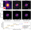 |
Fig. 6. Dynamic range and image quality improvement through self-calibration. The top two panels a–f show the improvement of imaging quality over multiple self-calibration iterations, demonstrated at 112.6 MHz with 1 s time integration and 1 MHz frequency averaging. White contour are drawn at 0.5%, 1%, 5%, 10%, 20%, 30%, 50%, 70%, and 90% of the peak intensity. The dashed yellow contour represents −1% of the peak intensity. The red ellipse in the bottom-left corner of each panel indicates the restoring beam. (a): Initial image (iteration 0), after applying only amplitude solutions from the calibrator and visibilities restricted to uv < 104 λ, allowing a simple Gaussian model to initiate phase-only self-calibration. (b): Image after first phase-only self-calibration using the Gaussian model; dynamic range (DR) improves to 106. (c): Phase-only self-calibration extended to uv < 254 λ for the second iteration further improves DR to 211. (d): After including baselines up to uv < 704 λ at iteration 5, DR increases to 343. (e): Final phase-only iteration with DR = 364. (f): Final image after amplitude-phase self-calibration converges; DR reaches 471. Bottom panel: Dynamic range variations across self-calibration cycles. Each point represents an iteration, and the maximum baseline length used (uvmax) is indicated in the figure. Phase-only calibration steps are shown in blue and yellow, amplitude-phase steps in red. Star markers indicate the best dynamic range achieved in each stage. The improvement in image fidelity through iterative self-calibration is evident. |
5.4. Solar disc alignment through quiet solar time
At low radio frequencies, variations in ionospheric electron density cause the apparent position of the Sun to drift over time and frequency. Self-calibration, while effective in correcting relative gain errors across the array, cannot provide absolute phase information. This process inherently loses absolute positional information on the sky. When self-calibration is applied under these conditions, the combined effect can result in significant misregistration of the Sun in the image plane.
To address this, self-calibration is performed on a short (1−2 s) duration of data during a quiet solar period, when the solar disc is clearly visible. In the initial iteration, a Gaussian model placed at the phase centre is used to ensure that the solar centre aligns with the phase centre. This step helps preserve the correct solar position, allowing the resulting images to be accurately transformed to the helioprojective coordinate system, which is essential for comparing solar radio images to those obtained at other wavebands. The ability to image the solar disc, and hence identify a quiet interval, is critical for correct registration of the radio image. If only a compact feature located away from the disc centre is visible, this method will incorrectly align that feature to the phase centre. The quiet-time selection follows the procedure in Section 5.1, but is applied to a maximum time span of 2 s.
5.5. Flagging solar observations
Flagging solar radio datasets poses a unique challenge: automated flagging algorithms that detect statistical outliers in time and frequency often misidentify genuine solar emissions, such as solar radio bursts, as RFI. This occurs because solar radio bursts are statistically indistinguishable from RFI in the time-frequency phase space. To address this issue, SIMPL implements a flagging strategy based on identifying outliers in the uv-domain independently for each time and frequency slice. This approach is effective even for transient solar radio emissions and has been implemented in the flagger ankflag (Kansabanik et al. 2023). For ease of integration, SIMPL uses a custom implementation inspired by ankflag, optimised for computational efficiency and minimisation of over-flagging. Details are provided below.
The Sun is a spatially complex and time-variable source, resulting in significant variations in visibility amplitudes across the uv-plane. The dominant trend is that the amplitudes at shorter uv-distances (corresponding to large angular scales) are significantly higher than at longer uv-distances. To ensure a meaningful statistical analysis, we performed logarithmic binning in uv-distance. This binning scheme uses finer bins at shorter uv-ranges – where visibility amplitudes are generally higher and vary rapidly – and coarser bins at longer uv-ranges, aligning well with the natural distribution of data density in the uv-plane. The flagging algorithm implemented in SIMPL treats the real and imaginary components of complex visibilities as independent statistical populations. They are analysed separately for each time-frequency slice using identical uv-binning and statistical analysis. Within each uv bin, robust statistical outlier detection is performed using median absolute deviation (MAD) with a deliberately lenient adaptive threshold. This threshold is typically 3 − 5σ, depending on the number of data points in the bin, and progressively increases for bins with fewer data points, e.g. 7.5σ for bins containing fewer than 20 data points. For a dataset X = {x1, x2, …, xn} in each uv-bin, a deviation score d is estimated as
 (5)
(5)
where M is the median(X). Points are flagged if the value of d for the real or imaginary component exceeds the threshold in its respective uv-bin. To prevent over-flagging, if more than 40% of points in any uv-bin are identified for flagging, the algorithm applies a more relaxed threshold (2× the original). If, despite this, the number of points to be flagged remains greater than 40%, no data are flagged for that uv-bin. For bins with more than 30 data points, the median calculation uses a trimmed estimator (removing 5% from each tail) to enhance robustness against contamination. Flagging is performed on the entire solar dataset, independently for each time, frequency, and correlation (XX and YY), on the CORRECTED_DATA column after self-calibration solutions have been applied, with parallel processing across multiple timestamps for faster processing.
This approach allows SIMPL to effectively flag outliers even in the presence of spectrally complex and temporally variable active solar emissions often seen in solar dynamic spectra. Figure 7c shows an example of flagging based on MAD applied to visibilities for a time and frequency slice severely affected by RFI. Panel a shows the image formed (with self-calibration applied) before this flagging. The image has an rms of 13.7 Jy/beam and a dynamic range of 37. Panel b shows the image obtained after flagging followed by self-calibration. The resulting image has an rms of 7.5 Jy/beam and a dynamic range of 74, representing approximately a factor of two improvement.
 |
Fig. 7. uv-domain based flagging on solar visibilites. Panels a and b show solar images at the same frequency and time, before and after SIMPL’s uv-based flagging, respectively. These are at 111.13 MHz with 1 s time integration and 195.3 kHz frequency averaging, and are severely affected by RFI. For panels a and b, white contours are drawn at 5%, 10%, 20%, 30%, 50%, 70%, and 90% of the peak intensity and the dashed yellow contour represents the −5% of the peak intensity. The restoring beam is show in red in the bottom-left corners. Image a exhibits an rms of 13.7 Jy/beam and a dynamic range of 37, while the image b, obtained after outlier flagging followed by another round of self-calibration, shows an improved rms of 7.5 Jy/beam and a dynamic range of 74. Panel c illustrates the corresponding visibility amplitudes as a function of uv-distance. Flagged visibilities (red) were identified as outliers as detailed in Section 5.5. This approach enables effective suppression of corrupted visibilities while preserving genuine solar structure across spatial scales. |
5.6. Spectroscopic snapshot imaging of solar emissions
The visibilities are corrected for beam gains towards the Sun once all preceding calibration steps are completed. This is performed using the everybeam4 module integrated within the DP3 framework. Spectroscopic snapshot imaging is then carried out using WSClean (Offringa et al. 2014). By default, imaging uses a Briggs weighting scheme with a robustness parameter of 0.5, which the user can adjust depending on the desired trade-off between sensitivity and resolution. Additional WSClean parameters have been empirically optimised through extensive testing across a variety of LOFAR solar datasets. Imaging is performed at user-defined time and frequency intervals and integrations, generating high-fidelity spectroscopic snapshot images of dynamic solar emission.
5.7. Optional higher dynamic range mode
In its default configuration, SIMPL partitions the measurement set into user-defined time and frequency chunks. Self-calibration solutions are computed independently for each chunk (using 1−2 s from within that chunk) and applied uniformly within it. A quiet period is preferred to correct for ionospheric refraction (Section 5.4), and longer time chunks increase the likelihood of including a suitably quiet interval. This approach offers ease of implementation, computational efficiency, and generally delivers imaging quality superior to that provided by earlier attempts. However, during periods of high ionospheric activity, calibration solutions can evolve significantly within an individual time chunk, reducing the benefits of this approach. This effect is naturally more pronounced for LBA than for HBA. Under such circumstances, reducing the time chunk size can improve the calibration accuracy and, consequently, the imaging quality.
Ionospheric activity tends to be higher during periods of higher solar activity. Periods of high solar activity require examining longer time chunks to find instances of acceptably low solar activity. Conversely, managing faster ionospheric variations requires working with shorter time chunks. The pipeline (SIMPL) first computes self-calibration solutions from the quietest time data available in a suitably large time chunk and applies them to the entire chunk to determine refractive shifts (Section 5.3). This is followed by optionally estimating self-calibration solutions for each time and frequency slice. Since the initial self-calibration provides a reliable starting model, this differential self-calibration stage bypasses Gaussian modelling and progressive baseline inclusion and starts with phase-only self-calibration, followed by amplitude and phase calibration until convergence is achieved. After convergence, the availability of a reliable model also enables residual-based RFI flagging, further enhancing image quality. Although advantageous for image quality, this approach presents computational challenges.
Figure 8 illustrates the improvement in imaging fidelity achieved through this two-step calibration process. Panel a shows the image obtained after the initial self-calibration using longer time and wider frequency chunks. While the dominant solar emission is well detected, residual phase errors cause elevated noise and degrade the dynamic range. Panel b shows the same time and frequency slice after performing differential self-calibration at full time and frequency resolution. The dynamic range improves by more than a factor of five, and some previously undetectable fainter sources – such as source two – are now clearly visible. This demonstrates the utility of differential self-calibration for capturing the complexity of solar emission morphology in greater detail, even under dynamic ionospheric and solar conditions, without compromising the positional alignment established during initial calibration.
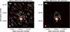 |
Fig. 8. Demonstration of SIMPL’s optional higher dynamic range mode on a LBA dataset. Panel a shows an image of a type II solar radio burst at 77 MHz, obtained with 195.3 kHz frequency averaging and 1 s time integration, following initial self-calibration on longer time and frequency intervals. This image, before differential self-calibration, has a dynamic range (DR) of 86. Panel b shows an image of the same type II burst at the same time and frequency after subsequent differential self-calibration, illustrating significant improvement in imaging fidelity with DR 467. The cyan circle denotes the optical solar disc. Contours are drawn at 1%, 3%, 5%, 10%, 20%, 30%, 50%, 70%, and 90% of the peak intensity. The restoring beam is shown in red in the bottom-left corner of each panel. The enhanced DR has enabled reliable detection of the faint source (marked 2), which is an order of magnitude fainter than source 1. |
6. Results
We implemented the algorithm described in Section 5 within SIMPL and applied it to multiple LOFAR datasets spanning a range of solar conditions to evaluate its performance and robustness. The pipeline is currently configured to operate in two distinct modes: one optimised to maximise imaging quality without regard to computational efficiency, and the other that prioritises faster runtimes by performing self-calibration on fewer time and frequency slices. In this section, we present the results produced by the computationally efficient mode. Figure 9 shows a representative sample of the resulting spectroscopic snapshot images.
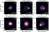 |
Fig. 9. Examples of spectroscopic snapshot images produced by SIMPL in its default mode. All images are generated using 1 s integration and 195.3 kHz frequency averaging, except for panel d, which was integrated over 1 s and 1 MHz. Contours are drawn at 3%, 5%, 10%, 20%, 30%, 50%, 70%, and 90% of the maximum intensity in each image. The red ellipse in the bottom-left corner of each panel indicates the restoring beam, and the dashed cyan circles represent the optical solar disc. Top panels a–c: HBA observations. Panels a and c show examples of noise storm emission. Panel b displays a bright type III radio burst, more than an order of magnitude more intense than the noise storm in panel a. Low-level contours reveal the quiet Sun emission even in the presence of strong radio sources. Bottom panels d–f: LBA observations. Panel d shows a quiet Sun snapshot at 35.64 MHz with a dynamic range of 104. Panels e and f correspond to snapshots immediately before and during a type II burst. The quiet Sun remains visible in the low-level contours, even in panel f, despite the presence of an intense burst. |
Panels a–c display HBA observations, demonstrating SIMPL’s ability to recover diverse solar emission features. In panels a and c, compact sources associated with noise storm activity are visible, with surrounding contours revealing extended quiet-Sun emission. Panel b showcases a strong type III radio burst, where the peak flux density exceeds that of the noise storm event shown in panel a by more than an order of magnitude. The pipeline recovers not only the intense type III burst, but also the noise storm region and the underlying quiet-Sun structure. The dynamic range achieved for HBA datasets routinely exceeds 400 under quiescent conditions and can exceed 1000 during intense radio bursts. The resulting images show well-defined source morphology with minimal imaging artefacts, even in the presence of rapidly evolving emission.
Panels d–f illustrate SIMPL’s performance at lower frequencies using LBA data. Panel d shows a quiet Sun snapshot at 35.64 MHz (integrated over 1 s and 1 MHz), demonstrating a dynamic range of approximately 100, with the 3% contour extending to ∼2.5 R⊙. Snapshot imaging of extended emissions is significantly more challenging than imaging compact sources, particularly with LOFAR LBA, which provides only 276 independent baselines when considering core stations alone. Previous quiet-Sun studies at these frequencies required 2−5 hours of integration (e.g. Zhang et al. 2022a). Panels e and f present 1 s, 195.3 kHz snapshot images capturing the onset of a type II radio burst, and panel e shows the quiet-Sun emission before the event. Despite the bright and structured emission in panel f, the quiet Sun remains visible in the lower contour levels. These examples highlight SIMPL’s ability to observe low-surface-brightness features with high fidelity, even in the presence of much brighter transient events.
Across both HBA and LBA observations, SIMPL consistently delivers high-quality spectroscopic snapshot images, achieving over an order of magnitude improvement in dynamic range compared to approaches that rely solely on calibration solutions obtained towards the calibrator source – used by earlier LOFAR imaging pipelines (Figure 3). The imaging quality is maintained over a wide frequency range (35−190 MHz), varying solar activity levels, and different observing epochs and solar conditions, underscoring the generality and robustness of the approach.
7. Integration in the existing processing framework
The LOFAR Solar and Space Weather key science project has recently undertaken a large-scale effort to reprocess the archival solar observations from LOFAR. In particular, the Incremental Development of LOFAR Space-weather (IDOLS; Zhang et al. 2022b) campaign, which routinely collects continuous solar and ionospheric observations, has led to a substantial increase in data volume, necessitating automated scheduling of the data reduction pipeline to provide higher-level data products without manual intervention. The framework used is called Apertif Task Database for the LOFAR Data Valorization (ATDB-LDV; Vermaas et al. 2019; Bozkurt et al. 2024), which orchestrates data retrieval from the archive, execution of the specified pipeline, and archival of processed data products. The ATDB-LDV framework supports the execution of pipelines described in the Common Workflow Language (CWL5). This structure supports flexible specification of pipeline parameters, execution strategies, and portability. Given SIMPL’s capability to calibrate both HBA and LBA interferometric datasets, we have implemented a CWL specification for the pipeline6, enabling its automatic execution on the LOFAR Solar archive and producing final data products including images and video previews.
8. Future development plans
Although the current implementation of SIMPL is optimised for processing large datasets, several improvements are planned to enhance its performance and functionality. As described in Sections 5.3 and 5.7, SIMPL currently offers two self-calibration modes: the default efficient mode, in which a self-calibration solution is computed only for a single carefully chosen time-frequency patch per chunk and applied to the entire chunk, and an optional mode in which an additional self-calibration solution is computed for each individual time and frequency slice being imaged. The former is computationally lean and delivers good imaging quality except during periods of enhanced ionospheric activity, whereas the latter delivers improved imaging quality, especially under challenging ionospheric conditions, but at significantly higher computational cost. An optimal approach to provide enhanced imaging quality without incurring excessive computational cost is to compute self-calibration solutions over a user-defined time-frequency grid, sufficiently fine to capture ionospheric variations in antenna gains, but much coarser than the imaging time-frequency integrations. Suitably interpolated calibration solutions can then be applied to the entire dataset. We plan to implement this mode as the default configuration in SIMPL as this strategy will retain most of the benefits of per-slice calibration but at a fraction of the associated computational cost.
We also plan to introduce two major new capabilities. While SIMPL represents a significant improvement over previous approaches, its current implementation does not fully exploit LOFAR’s capability in two key respects. First, although LOFAR can provide full polarimetric data, SIMPL is designed to produce only Stokes I (total intensity) images; second, SIMPL uses only the LOFAR core stations within a 2 km region and ignores the remote stations, which offer baselines up to ∼100 km. To extract the most information from the data, we intend to address both these limitations in future developments, as described in the following subsections.
8.1. Polarisation calibration
Full-Stokes calibration at low radio frequencies presents several challenges. Firstly, few bright, polarised calibrator sources are observable during the daytime; even at night, the number of well-characterised polarised sources at low radio frequencies remains small. Additionally, ionospheric Faraday rotation can introduce large and rapidly varying polarisation angle shifts, further complicating calibration.
A promising approach to address has recently been proposed by Kansabanik et al. (2025), who have developed a formalism leveraging the fact that an intrinsically unpolarised sky appears polarised due to instrumental beam polarisation. This induced polarisation can be modelled and used to derive accurate polarisation calibration solutions. We plan to integrate this method into SIMPL, along with solar-specific polarisation calibration strategies similar to those of Kansabanik et al. (2022), to enable spectro-polarimetric snapshot imaging of the Sun with LOFAR.
8.2. Incorporation of remote baselines
High-angular-resolution imaging of solar radio emissions is beginning to reveal the fine-scale structure of active regions and offers new avenues to probe coronal scattering and plasma processes (e.g. Mercier et al. 2015; Mondal et al. 2024, 2025; Morosan et al. 2025). LOFAR, with its remote baselines extending up to ∼100 km, offers immense potential for this science.
The foremost challenge, however, is that the correlated solar flux density decreases substantially even before 1000 λ, becoming extremely low on longer baselines. This limitation is compounded by the higher system temperature during solar observations, which further reduces the signal-to-noise ratio. Another difficulty arises from ionospheric phase variations, which differ significantly across long baselines, as antennas at larger separations sample different ionospheric patches (Lonsdale 2005). The self-calibration strategy implemented in SIMPL–based on iterative inclusion of progressively longer baselines–has proven effective for arrays with dense uv-coverage (Kansabanik 2022). However, applying this approach to LOFAR’s remote baselines is ineffective due to their sparse uv-sampling and the associated spatially variable ionospheric distortions. To address this, we are exploring methods to extend SIMPL beyond the core antennas by constructing reliable initial model of the Sun. One approach involves transferring calibration solutions from nighttime calibrator observations, when ionospheric conditions are more stable. Under favourable circumstances, these transferred solutions can potentially serve as a starting point for subsequent self-calibration. The development and validation of this methodology is currently in progress.
9. Conclusion
We have presented SIMPL, a fully automated, self-calibration-based imaging pipeline developed for LOFAR solar observations. This development was motivated by the need to address the inadequacies of standard calibrator-based approaches arising from the solar contamination of simultaneously observed calibrator sources and the direction-dependent nature of ionospheric phases. The pipeline addresses these issues by combining tailored strategies such as optimal calibrator time identification, uv-based flagging of solar data, and iterative self-calibration with gradual increases in model complexity. This has resulted in an order of magnitude improvement in dynamic range and a corresponding enhancement in imaging fidelity. While the current version of SIMPL focuses on Stokes I imaging and excludes remote baselines, future developments will extend its capabilities to full-polarisation imaging and high-resolution mapping using LOFAR’s remote stations. These additions will substantially improve our ability to probe solar radio phenomena across a broader span of spatial and polarisation phase space.
Despite their well-recognised scientific potential (e.g. Cairns 2004; Oberoi & Kasper 2004), solar radio images remain underutilised by the broader solar physics community. This is largely due to the absence of robust, feature-rich analysis toolkits and the steep learning curve associated with adapting generic radio-interferometric tools for solar applications. The pipeline directly addresses these barriers by delivering reliable high-time- and frequency-resolution spectroscopic snapshot images of the Sun, ready for scientific analysis without requiring specialised expertise in radio interferometry. It is currently being used to process more than a decade of LOFAR solar interferometric observations, producing science-ready FITS images for open access by the community. By lowering the technical barriers, SIMPL encourages broader participation from the solar community and will enable greater integration of solar radio imaging in multi-wavelength studies.
With LOFAR 2.0 on the horizon and the Square Kilometre Array Observatory soon to follow, providing the community access to high-quality, science-ready solar radio imaging is increasingly important. Maximising the scientific return from these upcoming facilities will require active participation from a diverse, global community that transcends traditional disciplinary boundaries, and tools such as SIMPL will be instrumental in achieving this goal.
Data availability
The Solar IMaging Pipeline for LOFAR (SIMPL) is publicly available at https://git.astron.nl/ssw-ksp/simpl
Acknowledgments
S.D., D.O. and D.P. acknowledge support from the Department of Atomic Energy, under project 12-R&D-TFR-5.02-0700. This paper is based on data obtained with the International LOFAR Telescope (ILT). LOFAR (van Haarlem et al. 2013) is the Low Frequency Array designed and constructed by ASTRON. It has observing, data processing, and data storage facilities in several countries, that are owned by various parties (each with their own funding sources), and that are collectively operated by the ILT foundation under a joint scientific policy. The ILT resources have benefitted from the following recent major funding sources: CNRS-INSU, Observatoire de Paris and Université d’Orléans, France; BMBF, MIWF-NRW, MPG, Germany; Science Foundation Ireland (SFI), Department of Business, Enterprise and Innovation (DBEI), Ireland; NWO, The Netherlands; The Science and Technology Facilities Council, UK; Ministry of Science and Higher Education, Poland. We thank the project LOFAR Data Valorization (LDV) [project numbers 2020.031, 2022.033, and 2024.047] of the research programme Computing Time on National Computer Facilities using SPIDER that is (co-)funded by the Dutch Research Council (NWO), hosted by SURF through the call for proposals of Computing Time on National Computer Facilities. We also thank SURF SARA with the project EINF-13633, Science ready products for LOFAR Solar, Heliospheric and ionospheric datasets.
References
- Anderson, M. M., Hallinan, G., Eastwood, M. W., et al. 2018, ApJ, 864, 22 [Google Scholar]
- Bhunia, S., Carley, E. P., Oberoi, D., & Gallagher, P. T. 2023, A&A, 670, A169 [NASA ADS] [CrossRef] [EDP Sciences] [Google Scholar]
- Bozkurt, A., Orru, E., Holties, H., et al. 2024, Proc. SPIE, 13098, 130982P [Google Scholar]
- Breitling, F., Mann, G., Vocks, C., Steinmetz, M., & Strassmeier, K. G. 2015, Astron. Comput., 13, 99 [NASA ADS] [CrossRef] [Google Scholar]
- Broekema, P. C., Mol, J. J. D., Nijboer, R., et al. 2018, Astron. Comput., 23, 180 [NASA ADS] [CrossRef] [Google Scholar]
- Bröse, M., Vocks, C., Warmuth, A., et al. 2025, A&A, 694, A188 [NASA ADS] [CrossRef] [EDP Sciences] [Google Scholar]
- Cairns, I. H. 2004, Planet. Space Sci., 52, 1423 [Google Scholar]
- CASA Team (Bean, B., et al.) 2022, PASP, 134, 114501 [NASA ADS] [CrossRef] [Google Scholar]
- Chhabra, S., Gary, D. E., Hallinan, G., et al. 2021, ApJ, 906, 132 [NASA ADS] [CrossRef] [Google Scholar]
- Clarkson, D. L., Kontar, E. P., Vilmer, N., et al. 2023, ApJ, 946, 33 [NASA ADS] [CrossRef] [Google Scholar]
- Cornwell, T. J., & Wilkinson, P. N. 1981, MNRAS, 196, 1067 [NASA ADS] [Google Scholar]
- Dabrowski, B., Wolowska, A., Vocks, C., et al. 2025, Acta Geophys., 73, 987 [Google Scholar]
- de Gasperin, F., Vink, J., McKean, J. P., et al. 2020, A&A, 635, A150 [NASA ADS] [CrossRef] [EDP Sciences] [Google Scholar]
- Dey, S., Kansabanik, D., Oberoi, D., & Mondal, S. 2025, ApJ, 988, L73 [Google Scholar]
- Hallinan, G., Anderson, M., Isella, A., et al. 2023, Am. Astron. Soc. Meet. Abstr., 241, 451.09 [Google Scholar]
- Kansabanik, D. 2022, Sol. Phys., 297, 122 [Google Scholar]
- Kansabanik, D., Oberoi, D., & Mondal, S. 2022, ApJ, 932, 110 [Google Scholar]
- Kansabanik, D., Bera, A., Oberoi, D., & Mondal, S. 2023, ApJS, 264, 47 [Google Scholar]
- Kansabanik, D., Mondal, S., & Oberoi, D. 2024, ApJ, 968, 55 [Google Scholar]
- Kansabanik, D., Vourlidas, A., Dey, S., Mondal, S., & Oberoi, D. 2025, ApJS, 278, 26 [Google Scholar]
- Lonsdale, C. J. 2005, ASP Conf. Ser., 345, 399 [NASA ADS] [Google Scholar]
- McCauley, P. I., Cairns, I. H., White, S. M., et al. 2019, Sol. Phys., 294, 106 [NASA ADS] [CrossRef] [Google Scholar]
- McLean, D. J., & Labrum, N. R. 1985, Solar Radiophysics: Studies of Emission from the Sun at Metre Wavelengths (Cambridge: Cambridge University Press) [Google Scholar]
- Melrose, D. B. 1989, Sol. Phys., 120, 369 [Google Scholar]
- Mercier, C., & Chambe, G. 2009, ApJ, 700, L137 [Google Scholar]
- Mercier, C., & Chambe, G. 2015, A&A, 583, A101 [NASA ADS] [CrossRef] [EDP Sciences] [Google Scholar]
- Mercier, C., Subramanian, P., Chambe, G., & Janardhan, P. 2015, A&A, 576, A136 [NASA ADS] [CrossRef] [EDP Sciences] [Google Scholar]
- Mohan, A., Mondal, S., Oberoi, D., & Lonsdale, C. J. 2019, ApJ, 875, 98 [NASA ADS] [CrossRef] [Google Scholar]
- Mondal, S., Mohan, A., Oberoi, D., et al. 2019, ApJ, 875, 97 [NASA ADS] [CrossRef] [Google Scholar]
- Mondal, S., Oberoi, D., & Mohan, A. 2020a, ApJ, 895, L39 [NASA ADS] [CrossRef] [Google Scholar]
- Mondal, S., Oberoi, D., & Vourlidas, A. 2020b, ApJ, 893, 28 [NASA ADS] [CrossRef] [Google Scholar]
- Mondal, S., Oberoi, D., Biswas, A., & Kansabanik, D. 2023, ApJ, 953, 4 [Google Scholar]
- Mondal, S., Kansabanik, D., Oberoi, D., & Dey, S. 2024, ApJ, 975, 122 [Google Scholar]
- Mondal, S., Zhang, P., Kansabanik, D., Oberoi, D., & Pearce, G. 2025, Sol. Phys., 300, 109 [Google Scholar]
- Morosan, D. E., Gallagher, P. T., Zucca, P., et al. 2015, A&A, 580, A65 [NASA ADS] [CrossRef] [EDP Sciences] [Google Scholar]
- Morosan, D. E., Carley, E. P., Hayes, L. A., et al. 2019, Nat. Astron., 3, 452 [Google Scholar]
- Morosan, D. E., Jebaraj, I. C., Zhang, P., et al. 2025, A&A, 695, A70 [NASA ADS] [CrossRef] [EDP Sciences] [Google Scholar]
- Nindos, A. 2020, Front. Astron. Space Sci., 7, 57 [NASA ADS] [CrossRef] [Google Scholar]
- Oberoi, D., & Kasper, J. C. 2004, Planet. Space Sci., 52, 1415 [Google Scholar]
- Oberoi, D., Sharma, R., & Rogers, A. E. E. 2017, Sol. Phys., 292, 75 [Google Scholar]
- Oberoi, D., Bisoi, S. K., Sasikumar Raja, K., et al. 2023, JApA, 44, 40 [Google Scholar]
- Offringa, A. R., McKinley, B., Hurley-Walker, N., et al. 2014, MNRAS, 444, 606 [Google Scholar]
- Pearson, T. J., & Readhead, A. C. S. 1984, ARA&A, 22, 97 [Google Scholar]
- Pick, M., & Vilmer, N. 2008, A&ARv, 16, 1 [NASA ADS] [CrossRef] [Google Scholar]
- Ratcliffe, H., Kontar, E. P., & Reid, H. A. S. 2014, A&A, 572, A111 [NASA ADS] [CrossRef] [EDP Sciences] [Google Scholar]
- Saint-Hilaire, P., Vilmer, N., & Kerdraon, A. 2013, ApJ, 762, 60 [NASA ADS] [CrossRef] [Google Scholar]
- Sharma, R., Oberoi, D., Battaglia, M., & Krucker, S. 2022, ApJ, 937, 99 [NASA ADS] [CrossRef] [Google Scholar]
- Suresh, A., Sharma, R., Oberoi, D., et al. 2017, ApJ, 843, 19 [CrossRef] [Google Scholar]
- Tingay, S. J., Oberoi, D., Cairns, I., et al. 2013, J. Phys. Conf. Ser., 440, 012033 [Google Scholar]
- van Diepen, G., Dijkema, T. J., & Offringa, A. 2018, Astrophysics Source Code Library [record ascl:1804.003] [Google Scholar]
- van Haarlem, M. P., Wise, M. W., Gunst, A. W., et al. 2013, A&A, 556, A2 [NASA ADS] [CrossRef] [EDP Sciences] [Google Scholar]
- Vermaas, N., Moss, V., & de Goei, R. 2019, Astronomical Data Analysis Software and Systems XXIX [Google Scholar]
- Vocks, C., Mann, G., Breitling, F., et al. 2018, A&A, 614, A54 [NASA ADS] [CrossRef] [EDP Sciences] [Google Scholar]
- Wayth, R. B., Tingay, S. J., Trott, C. M., et al. 2018, PASA, 35, e033 [NASA ADS] [CrossRef] [Google Scholar]
- Zhang, P., Zucca, P., Kozarev, K., et al. 2022a, ApJ, 932, 17 [CrossRef] [Google Scholar]
- Zhang, P., Zucca, P., Kozarev, K. A., Gallagher, P., & Nedal, M. 2022b, AGU Fall Meeting Abstracts, 2022, SH35E–1844 [Google Scholar]
- Zhang, P., Morosan, D., Kumari, A., & Kilpua, E. 2024, A&A, 683, A123 [NASA ADS] [CrossRef] [EDP Sciences] [Google Scholar]
- Zucca, P., Morosan, D. E., Rouillard, A. P., et al. 2018, A&A, 615, A89 [NASA ADS] [CrossRef] [EDP Sciences] [Google Scholar]
- Zucca, P., Zhang, P., Kozarev, K., et al. 2025, A&A, 703, A271 [NASA ADS] [CrossRef] [EDP Sciences] [Google Scholar]
All Figures
|
Fig. 1. Instantaneous uv-coverage comparison between the LOw Frequency ARray (LOFAR) and the Murchison Widefield Array (MWA). Projected baseline distributions are shown for (a) LOFAR-LBA, (b) LOFAR-HBA, and (c) the MWA Phase-II configuration. Both LOFAR-LBA and HBA exhibit densely clustered cores, providing high sensitivity to large-scale solar structures, complemented by longer remote baselines that enable higher spatial resolution. In contrast, the MWA provides a significantly denser and more uniformly distributed uv-coverage within a compact footprint, facilitating high-fidelity snapshot imaging at moderate resolution (a few arcminutes). Insets in each panel zoom into the central ±2 km region (marked by red squares) to highlight baseline distributions within the core. The dashed black circles indicate radii of 2.5, 5, 10, 20, and 50 km. The number of independent baselines from core antennas is 276 for LOFAR-LBA and 1128 for LOFAR-HBA. For panel c, representing the MWA phase-II configuration, there are 8128 instantaneous baselines within 5 km. |
| In the text | |
|
Fig. 2. Comparison of dynamic spectra (DS) from the Sun (a) and the calibrator Cassiopeia A (b), observed simultaneously with two separate LOFAR station beams. These DS were generated by averaging visibilities in the 150−500 λ range in the uv-plane to preferentially capture transient, compact structures while suppressing contributions from large-scale quiet Sun emission. Although Cassiopeia A was located 11.4° from the Sun during the observation, its DS shows features that strongly resemble those seen in the solar spectrum, indicating substantial solar contamination in the calibrator field. This highlights the difficulty of obtaining clean calibrator data during solar observing sessions, particularly with wide field of view (FoV) instruments such as LOFAR. |
| In the text | |
|
Fig. 3. Limitations of applying calibrator-based phase solutions across widely separated sky regions. Left panel: Image of Virgo A obtained using calibration solutions from the calibrator beam, demonstrating excellent fidelity and a dynamic range exceeding 1250 (rms: 0.08 Jy/beam). Middle panel: Solar image obtained by applying calibration solutions derived from the calibrator source Virgo A. The image suffers from significant phase errors, resulting in distorted morphology and a limited dynamic range of ∼28 (rms: 4.0 Jy/beam). Right panel: Solar image produced by the SIMPL pipeline using a self-calibration-based approach, yielding a markedly improved dynamic range of ∼550 (rms: 0.5 Jy/beam). Contours at each panel are drawn at −1%, 1%, 5%, 10%, 20%, 30%, 50%, 70%, and 90% of their respective peaks, with the negative contour shown as dashed yellow lines. The red ellipse in the bottom-left corner of each panel indicates the restoring beam. The comparison underscores the necessity of direction-dependent calibration for accurate high-fidelity solar imaging. |
| In the text | |
|
Fig. 4. Schematic overview of SIMPL. The flow is divided into three main sections: calibrator processing (orange), solar processing (light blue), and the self-calibration sub-module (darker blue). Calibrator processing identifies an optimal quiet time range for daytime observations, derives antenna gain solutions, and applies only the amplitude part of the gains to solar data. Solar processing operates on time–frequency chunks of the solar measurement set, invoking the self-calibration block to iteratively refine phase (and later amplitude) solutions. An optional higher dynamic range mode estimates differential self-calibration solutions per time and frequency slice. Final steps include primary beam correction and generation of spectroscopic snapshot images. Rounded rectangles denote processing steps, diamonds represent decision points, and dashed rounded rectangles indicate iterative self-calibration loops. |
| In the text | |
|
Fig. 5. Automated identification of a quiet calibration interval within contaminated calibrator data. The top panel shows the dynamic spectra of a calibrator observation (Cassiopeia A) contaminated by solar emission, with vertical dashed cyan lines marking the start and end of the automatically identified quiet interval. The bottom panel displays the smoothed composite score time series, derived from statistical measures of variability, non-Gaussianity, and entropy across sliding time windows. The horizontal green line marks the 25th percentile threshold used to define ‘quiet’ intervals. The selected segment (between red dashed lines, from 13:48:20 to 13:50:18 UTC) represents the longest continuous window below this threshold and is used for reliable calibration. |
| In the text | |
|
Fig. 6. Dynamic range and image quality improvement through self-calibration. The top two panels a–f show the improvement of imaging quality over multiple self-calibration iterations, demonstrated at 112.6 MHz with 1 s time integration and 1 MHz frequency averaging. White contour are drawn at 0.5%, 1%, 5%, 10%, 20%, 30%, 50%, 70%, and 90% of the peak intensity. The dashed yellow contour represents −1% of the peak intensity. The red ellipse in the bottom-left corner of each panel indicates the restoring beam. (a): Initial image (iteration 0), after applying only amplitude solutions from the calibrator and visibilities restricted to uv < 104 λ, allowing a simple Gaussian model to initiate phase-only self-calibration. (b): Image after first phase-only self-calibration using the Gaussian model; dynamic range (DR) improves to 106. (c): Phase-only self-calibration extended to uv < 254 λ for the second iteration further improves DR to 211. (d): After including baselines up to uv < 704 λ at iteration 5, DR increases to 343. (e): Final phase-only iteration with DR = 364. (f): Final image after amplitude-phase self-calibration converges; DR reaches 471. Bottom panel: Dynamic range variations across self-calibration cycles. Each point represents an iteration, and the maximum baseline length used (uvmax) is indicated in the figure. Phase-only calibration steps are shown in blue and yellow, amplitude-phase steps in red. Star markers indicate the best dynamic range achieved in each stage. The improvement in image fidelity through iterative self-calibration is evident. |
| In the text | |
|
Fig. 7. uv-domain based flagging on solar visibilites. Panels a and b show solar images at the same frequency and time, before and after SIMPL’s uv-based flagging, respectively. These are at 111.13 MHz with 1 s time integration and 195.3 kHz frequency averaging, and are severely affected by RFI. For panels a and b, white contours are drawn at 5%, 10%, 20%, 30%, 50%, 70%, and 90% of the peak intensity and the dashed yellow contour represents the −5% of the peak intensity. The restoring beam is show in red in the bottom-left corners. Image a exhibits an rms of 13.7 Jy/beam and a dynamic range of 37, while the image b, obtained after outlier flagging followed by another round of self-calibration, shows an improved rms of 7.5 Jy/beam and a dynamic range of 74. Panel c illustrates the corresponding visibility amplitudes as a function of uv-distance. Flagged visibilities (red) were identified as outliers as detailed in Section 5.5. This approach enables effective suppression of corrupted visibilities while preserving genuine solar structure across spatial scales. |
| In the text | |
|
Fig. 8. Demonstration of SIMPL’s optional higher dynamic range mode on a LBA dataset. Panel a shows an image of a type II solar radio burst at 77 MHz, obtained with 195.3 kHz frequency averaging and 1 s time integration, following initial self-calibration on longer time and frequency intervals. This image, before differential self-calibration, has a dynamic range (DR) of 86. Panel b shows an image of the same type II burst at the same time and frequency after subsequent differential self-calibration, illustrating significant improvement in imaging fidelity with DR 467. The cyan circle denotes the optical solar disc. Contours are drawn at 1%, 3%, 5%, 10%, 20%, 30%, 50%, 70%, and 90% of the peak intensity. The restoring beam is shown in red in the bottom-left corner of each panel. The enhanced DR has enabled reliable detection of the faint source (marked 2), which is an order of magnitude fainter than source 1. |
| In the text | |
|
Fig. 9. Examples of spectroscopic snapshot images produced by SIMPL in its default mode. All images are generated using 1 s integration and 195.3 kHz frequency averaging, except for panel d, which was integrated over 1 s and 1 MHz. Contours are drawn at 3%, 5%, 10%, 20%, 30%, 50%, 70%, and 90% of the maximum intensity in each image. The red ellipse in the bottom-left corner of each panel indicates the restoring beam, and the dashed cyan circles represent the optical solar disc. Top panels a–c: HBA observations. Panels a and c show examples of noise storm emission. Panel b displays a bright type III radio burst, more than an order of magnitude more intense than the noise storm in panel a. Low-level contours reveal the quiet Sun emission even in the presence of strong radio sources. Bottom panels d–f: LBA observations. Panel d shows a quiet Sun snapshot at 35.64 MHz with a dynamic range of 104. Panels e and f correspond to snapshots immediately before and during a type II burst. The quiet Sun remains visible in the low-level contours, even in panel f, despite the presence of an intense burst. |
| In the text | |
Current usage metrics show cumulative count of Article Views (full-text article views including HTML views, PDF and ePub downloads, according to the available data) and Abstracts Views on Vision4Press platform.
Data correspond to usage on the plateform after 2015. The current usage metrics is available 48-96 hours after online publication and is updated daily on week days.
Initial download of the metrics may take a while.