| Issue |
A&A
Volume 704, December 2025
|
|
|---|---|---|
| Article Number | A210 | |
| Number of page(s) | 13 | |
| Section | Extragalactic astronomy | |
| DOI | https://doi.org/10.1051/0004-6361/202557040 | |
| Published online | 10 December 2025 | |
Constraints on dark matter models from the stellar cores observed in ultra-faint dwarf galaxies
Self-interacting dark matter
1
Instituto de Astrofísica de Canarias, La Laguna, Tenerife E-38200, Spain
2
Departamento de Astrofísica, Universidad de La Laguna, Tenerife, Spain
★ Corresponding author: This email address is being protected from spambots. You need JavaScript enabled to view it.
Received:
29
August
2025
Accepted:
6
October
2025
Abstract
It has been proposed that the stellar cores observed in ultra-faint dwarf (UFD) galaxies reflect underlying dark matter (DM) cores that cannot be formed by stellar feedback acting on collisionless cold dark matter (CDM) halos. Assuming this claim is correct, we investigate the constraints that arise if such cores are produced by self-interacting dark matter (SIDM). We derive the range of SIDM cross sections (σ/m) required to reproduce the observed core sizes. These can result from halos in either the core-formation phase (low σ/m) or the core-collapse phase (high σ/m), yielding a wide range of allowed values (∼0.3–200 cm2 g−1) consistent with those reported in the literature for more massive galaxies. We also construct a simple model that relates stellar mass to core radius – two observables likely connected in SIDM. This model reproduces the stellar core sizes and masses in UFDs with σ/m values consistent with the above range. It also predicts a trend of increasing core radius with stellar mass, in agreement with observations of more massive dwarf galaxies. The model’s central DM densities match observations when assuming that the SIDM profile originates from an initial CDM halo that follows the mass–concentration relation. Since stellar feedback is insufficient to form cores in these galaxies, UFDs unbiasedly anchor σ/m at low velocities. If the core-collapse scenario holds (i.e., high σ/m), UFD halos are thermalized on kiloparsec scales, approximately two orders of magnitude larger than the stellar cores. These large thermalization scales could potentially influence substructure formation in more massive systems.
Key words: galaxies: dwarf / galaxies: evolution / galaxies: halos / galaxies: kinematics and dynamics / galaxies: stellar content / dark matter
© The Authors 2025
 Open Access article, published by EDP Sciences, under the terms of the Creative Commons Attribution License (https://creativecommons.org/licenses/by/4.0), which permits unrestricted use, distribution, and reproduction in any medium, provided the original work is properly cited.
This article is published in open access under the Subscribe to Open model. This email address is being protected from spambots. You need JavaScript enabled to view it. to support open access publication.
1. Introduction
The nature of dark matter (DM) remains one of the most pressing open questions in science1. In the standard cosmological model, dark matter (DM) is assumed to be cold and collisionless (CDM), consisting of particles that interact with baryons and with each other solely through gravity. While this model has proven remarkably successful, it is likely an effective approximation of a deeper, more complex reality in which DM exhibits some form of non-gravitational interaction. To advance our understanding, it is therefore crucial to explore potential tensions between CDM predictions and observational data (see this argument in, e.g., Silk 2017; Peebles 2021; Efstathiou 2025).
One notable tension that extends from the well-known core-cusp problem involves the DM distribution in the faintest galaxies. In cosmological simulations, self-gravitating CDM halos develop steep central density profiles, or cusps, which contrast with the approximately constant-density cores observed in many galaxies (e.g., Del Popolo & Le Delliou 2017; Bullock & Boylan-Kolchin 2017; Salucci 2019). According to the standard interpretation, the CDM cusps are transformed into cores through baryonic processes – such as feedback from star formation – that redistribute matter and alter the total mass profile, including the DM component (Governato et al. 2010; Pontzen & Governato 2012). However, the effectiveness of this mechanism depends on the availability of energy from star formation, and it becomes negligible below a stellar mass threshold of roughly 106 M⊙ (e.g., Peñarrubia et al. 2012; Tollet et al. 2016). Ultra-faint dwarf galaxies (UFDs), which have stellar masses well below this limit (e.g., Simon 2019; Battaglia & Nipoti 2022), are therefore expected to retain cuspy DM halos if the DM is CDM. Thus, the detection of DM cores in such systems, as recently reported by Sánchez Almeida et al. (2024a), deepens the core-cusp problem and points toward physics beyond the standard CDM paradigm.
Determining the DM distribution in the tiny UFDs is challenging and remains subject to significant uncertainty. Obtaining detailed kinematic data is difficult, so Sánchez Almeida et al. (2024a)’s recent claim relies instead on the fact that the stellar distributions of UFDs exhibit conspicuous cores. Under a set of defensible assumptions – such as non-tangentially biased velocities and axial symmetry – the Eddington inversion method allows one to demonstrate that a stellar core is physically inconsistent with a cuspy DM profile (An & Evans 2006; Sánchez Almeida et al. 2023, 2024b). This approach, implemented in the tool described by Sánchez Almeida et al. (2025), was applied to the surface density profiles of the six UFDs observed by Richstein et al. (2024), leading to the conclusion that these galaxies likely reside in cored DM potentials. Once alternative explanations – such as stellar feedback – are ruled out, the most compelling interpretation is that the DM departs from the standard CDM behavior.
Many physical models beyond CDM produce DM cores, for example, self-interacting DM (SIDM; Spergel & Steinhardt 2000), fuzzy DM (Schive et al. 2014), self-interacting fuzzy DM (Indjin et al. 2025), warm DM (Bode et al. 2001), Bose-Einstein condensate DM (Delgado & Muñoz Mateo 2023), fermionic DM (Argüelles et al. 2023), and late-time DM decay (Chu & Garcia-Cely 2018). The ease with which cores form is understandable given that cores are characteristic of self-gravitating systems approaching thermodynamic equilibrium (Plastino & Plastino 1993; Binney & Tremaine 2008; Sánchez Almeida 2022). Any physical process leading to the thermalization of the DM halo would develop a central core. What is truly remarkable about the CDM framework is that, due to the absence of non-gravitational interactions, halos fail to reach thermodynamic equilibrium within a Hubble time (tH) and instead retain memory of their initial conditions (e.g., Brown et al. 2020).
Although the formation of cores is a generic prediction, the constraints arising from the presence of DM cores in UFDs depend on the specific physical DM model and therefore need to be analyzed individually for each case. Here, we focus on the constraints applicable to SIDM models, in which DM particles undergo collisions beyond standard two-body gravitational interactions. This new interaction is characterized by a cross section sufficiently large to ensure that the DM halos of UFD galaxies thermalize within tH. SIDM represents the most straightforward conceptual extension of the standard CDM framework, introducing particle collisions that promote thermalization – much like molecular interactions establish thermodynamic equilibrium in the air. The concept was first introduced by Spergel & Steinhardt (2000) and has since gained considerable attention in the literature (e.g., Wandelt et al. 2001; Elbert et al. 2015; Tulin & Yu 2018; Adhikari et al. 2022), partly because self-interactions are a generic prediction of many particle physics DM models involving a hidden sector (e.g., Feng et al. 2009; Buckley & Fox 2010), and partly because of the profound impact that the reality of self-interactions would have in ruling out many popular DM particle candidates (e.g., Sarkar 2018).
The paper is organized as follows: Section 2 uses the scaling relation provided by Outmezguine et al. (2023) to work out the SIDM cross sections able to generate the cores observed in UFDs. They are compared with SIDM cross section estimates from the literature derived using a variety of methods, including gravitational lensing, galaxy cluster collisions, galaxy rotation curves, and dynamical modeling of dwarf galaxies. Section 3 uses the time evolution from cuspy to cored DM profiles, as modeled by Yang et al. (2024), to construct a toy model that relates the stellar core radius to the stellar mass of a galaxy for a given velocity-dependent SIDM cross section. According to this model, the stellar cores in UFDs require cross sections similar to those inferred in Sect. 2. Moreover, the model reproduces the trend of the stellar core radius increasing with stellar mass seen with other, more massive dwarfs from the literature. Cross sections consistent with the observed UFD cores can be small, if the DM halos are in the phase of forming a core, or large, if they are in the core-collapse phase. Both solutions are possible, but the physical mechanism giving rise to the DM distribution in the halo is different. Section 4 shows how only the DM particles forming the core have interacted during the core-formation phase, whereas the rest maintain the original distribution expected from collision-less CDM halos. In the core-collapse phase, however, the whole halo is in thermodynamic equilibrium, and so the stellar cores are tiny compared with the thermalization radii. Section 5 discusses and summarizes the results of the work. Appendices A and C detail the literature on cross sections and other properties of the galaxies used for contextualization, and Appendix B gives the stellar mass versus DM halo mass relation employed in the toy model. Appendix D shows how the stellar distribution observed in UFDs is well reproduced by the halo shape employed in Sect. 3 to construct the toy model.
2. Relating core radius with the SIDM cross section
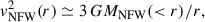
The constraints on the cross sections can be estimated keeping in mind that SIDM halos of all masses and sizes seem to follow the same time evolution once properly normalized to the characteristic timescale for the collision of two DM particles (Balberg et al. 2002; Loeb & Weiner 2011),
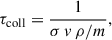 (1)
(1)
where σ, v, ρ, and m stand for the cross section, the relative velocities between DM particles, the characteristic volume density, and the DM particle mass, respectively. The universal behavior has been shown to hold under various assumptions including constant and velocity-dependent cross section (Balberg et al. 2002; Outmezguine et al. 2023; Yang et al. 2024). Figure 1 illustrates this universal time evolution as computed by Yang et al. (2024; Eq. (3.3)) from the N-body numerical simulation by Yang & Yu (2022) with σ = σ(v). The original NFW halos (Navarro et al. 1997) turn to form a core that expands while dropping the central density to a minimum value (Fig. 1a, the dashed lines, and Figs. 1c and 1d, the blue solid lines). From this time on, the DM–DM collisions trigger the core-collapse of the DM halo, which begins to contract; in doing so, its central density increases and it loses part of its core mass (e.g., Elbert et al. 2015; Outmezguine et al. 2023); see the solid lines in Fig. 1a. The scaling between σ and the true timescale driving the evolution of the system has to be found through numerical simulations. In the scanning of initial conditions computed by Outmezguine et al. (2023), they begin from DM halos with NFW profiles characterized by density ρs and length scale rs,
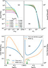 |
Fig. 1. Time evolution of SIDM halos according to Yang et al. (2024). The timescale is parameterized in terms of the core-collapse timescale, tcc – Eqs. (3) and (7). The halos start off as NFW profiles of characteristic density and radius ρs0 and rs0, respectively. (a) Radial density at different timesteps going from almost the initial conditions (tage/tcc = 0) to core-collapse (tage/tcc = 1), including the formation of a maximum core (tage/tcc = tc/tcc ≃ 0.12). Profiles before the maximum core formation (tage ≤ tc) are represented as dashed lines whereas profiles after this core-formation are shown as solid lines. (b) Same profiles as (a) but normalized to the central density and to the core radius defined in Eq. (6). The black bullet symbol indicates the location of the core radius. (c) Time variation of the true core (the blue solid line; rc in Eq. (17)) and of the model core (the orange dashed line; r′c in Eq. (15)). (d) Time variation of the central density (the blue solid line; ρSIDM(0)) and of the characteristic density (the orange dashed line; ρs′ in Eq. (15)). The green arrow in (c) and (d) marks the timescale for maximum core formation. |
 (2)
(2)
which evolve with time due to the DM self-collisions treated as heat conduction. Although initial DM halos may deviate from NFW profiles with somewhat steeper inner power-law slopes (e.g., Tasitsiomi et al. 2004; Delos & White 2023), the evolution of SIDM halos is likely insensitive to these initial conditions because DM particle self-interactions thermalize the distribution, leaving halo properties determined mainly by global quantities such as mass and energy (e.g., Sánchez Almeida 2022, and references therein). The characteristic timescale to reach the smallest density and the largest core radius (hereinafter, core-formation timescale) is found to be
 (3)
(3)
with the symbol C a numerical factor of order one introduced by the conductivity model representing the collisions. On the other hand, vmax is the maximum of the rotational velocity of the original NFW halo and so depends on rs and ρs as
 (4)
(4)
with G the gravitational constant. The SIDM cross section in Eq. (3) is an effective cross section that integrates over the halo characteristic velocities and provides a good approximation to self-scattering during the halo evolution (see Yang & Yu 2022; Outmezguine et al. 2023). To fit our needs, Eq. (3) can be rewritten as
![Mathematical equation: $$ \begin{aligned} t_{c} \simeq 2.5\,\mathrm{Gyr}\, \frac{0.6}{C}\, \frac{10\,\mathrm{cm^2\,g^{-1}}}{\sigma /m}\ \left[\frac{44\,M_\odot \,\mathrm{pc^{-2}}}{\rho _c(t_c)\,r_c(t_c)}\right]^{3/2} \left[\frac{r_c(t_c)}{50\,\mathrm{pc}}\right]^{1/2}, \end{aligned} $$](/articles/aa/full_html/2025/12/aa57040-25/aa57040-25-eq5.gif) (5)
(5)
where rc(tc) is the largest core radius; for the model analyzed by Outmezguine et al. (2023), it is just rc(tc)≃0.45 rs. Here and throughout, the core radius (rc) is implicitly defined as
 (6)
(6)
with ρ(r) the density profile. The symbol ρc(tc) stands for the smallest core density, reached when the radius is largest, which happen to be ρc(tc)≃2.4 ρs. The normalization of ρc(tc) rc(tc) to 44 M⊙ pc−2 was set because this product, for a large range of DM halo masses, has been observed to be approximately constant (Burkert 1995; Donato et al. 2009) with the value used in Eq. (5) (Sánchez Almeida 2025). After the formation of the core, the halo evolves to eventually core collapse (e.g., Binney & Tremaine 2008). The central density increases while the core shrinks to a point where they become similar to the original NFW cusp (Figs. 1c and 1d). According to Fig. 1c and the numerical simulations used to derive Eq. (3), this core-collapse occurs in a timescale on the order of
 (7)
(7)
Using these equations, we were able to estimate the cross section required to produce the cores observed in UFDs. Their halo must have developed a core but not yet have undergone full core-collapse. If tage is the age of such a halo, then the condition imposes
 (8)
(8)
with βage = tage/tH the age relative to the Hubble time. The lower limit in Eq. (8) comes from the assumption that cores are already formed at a time tc/2, which is consistent with the simulations (see Fig. 1a and Sect. 3). Equations (5), (7), and (8) can be combined to yield
 (9)
(9)
where the new symbol σH/m stands for
![Mathematical equation: $$ \begin{aligned} \sigma _H/m = 1.85\,\mathrm{cm^2 g^{-1}}\,\frac{0.6}{C}\, \left[\frac{44\,M_\odot \,\mathrm{pc^{-2}}}{\rho _c(t_c)\,r_c(t_c)}\right]^{3/2} \left[\frac{r_c(t_c)}{50\,\mathrm{pc}}\right]^{1/2}, \end{aligned} $$](/articles/aa/full_html/2025/12/aa57040-25/aa57040-25-eq10.gif) (10)
(10)
which is the cross section required to form the largest core of radius rc with density ρc in a Hubble time tH.
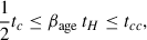
Figure 2 shows the range of cross sections permitted by Eq. (9) given the range of properties of the UFDs analyzed by Sánchez Almeida et al. (2024a). The distribution of the parameter σH/m/βage (gray histogram in Fig. 2) was obtained using a Monte Carlo simulation in which all unknown parameters were varied independently, each drawn from a uniform probability distribution within physically reasonable ranges. In particular, C was varied between 0.5 and 0.8, consistent with values from numerical simulations (e.g., Outmezguine et al. 2023), βage between 0.3 and 0.7, in line with DM halo ages reported in simulations (e.g., Lu et al. 2006; Correa et al. 2015), ρc(tc)rc(tc) between 10 and 100 M⊙ pc−2, as inferred from observations (e.g., Sánchez Almeida 2025), and rc(tc) between 20 and 60 pc, following the observational constraints of Sánchez Almeida et al. (2024a). According to Eq. (9), the cores can be produced with cross sections going from (σH/m/βage)/2, if the halos are forming the core (the blue histogram in Fig. 2), to (σH/m/βage)×8.5, if the halos are approaching core-collapse (the green histogram). Since we did not know whether the UFDs were forming their cores or core-collapsing, we considered the two possibilities to set limits on their cross section. Thus, σ/m has to be in the range
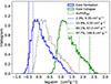 |
Fig. 2. Monte Carlo simulation used to estimate the SIDM cross sections required to account for the DM cores of UFDs. The cross sections depend on a number of poorly constrained parameters (the parameters in Eq. (10)). The Monte Carlo simulations allow us to propagate their uncertainties on σH/m/βage (the gray histogram) and, via Eq. (9), on the cross section σ/m. The blue histogram represents the distribution assuming the UFDs are in the process of forming the core, whereas the green histogram assumes that DM is evolving into the core-collapse phase. The vertical dashed lines mark the 2.3% and 97.7% percentiles used to constrain the range of viable cross sections given in Eq. (11). See the main text for further details. |
 (11)
(11)
which corresponds to the −2 SD (Standard Deviation) limit of the (σH/m/βage)/2 distribution (percentile 2.3%) and the +2 SD limit of the (σH/m/βage)×8.5 distribution (percentile 97.7%; see the dashed lines in Fig. 2). The interval in Eq. (11) can be written as
 (12)
(12)
To assign a velocity to the UFDs (veff) suitable to characterize the cross section, we followed Yang et al. (2024) which proposed
 (13)
(13)
with vmax given by Eq. (4). As in the analysis by Outmezguine et al. (2023) that led to Eq. (3), rc(tc)≃0.45 rs and ρc(tc)≃2.4 ρs; therefore, assuming ρc(tc) rc(tc) and rc(tc), one can determine vmax (Eq. (4)) and thus veff (Eq. (13)). The same Monte Carlo simulation providing the interval in Eq. (11) renders
 (14)
(14)
2.1. Comparison with existing estimates of σ/m
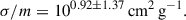
Figure 3 provides a summary of the current constraints and claims on the SIDM cross section found in the literature. The sources are quite diverse and there is no general rule on how σ/m and the velocity are computed from the observational data. We selected these cross sections from the papers that cited the seminal work of Randall et al. (2008), who set an upper limit on σ/m based on the lack of separation between DM and stars in the Bullet Cluster. The individual references are pointed out in Appendix A together with some general remarks on how each cross section was derived.
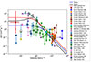 |
Fig. 3. SIDM cross sections found in the literature versus a representative relative velocity of the DM particles in the observed object. See Appendix A for the full references explaining that σ/m and “Velocity” have different meanings in the different works, which may explain part of the scatter. The value provided by the UFDs analyzed in this work is shown with the red circle with error bars. The two times symbols represent the median of the core formation and the core-collapse distributions shown in Fig. 2. The solid lines corresponds to the analytical form in Eq. (18), where σ0/m, w0, w1 = 30 cm2 g−1, 0, 80 km s−1 (the red line), 3 cm2 g−1, 0, 200 km s−1 (the blue line), and 11 cm2 g−1, 60 km s−1, 45 km s−1 (the black line). |
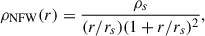
The constraints provided by the UFDs are incorporated into Fig. 3 as a single point, with error bars representing the range of possible cross sections. Specifically, the red circle with error bars at the lowest velocity corresponds to the cross section range given in Eq. (12), and to the velocity range defined by veff in Eq. (14). The two times symbols along the vertical error bar mark the median values of σ/m obtained from the core-formation and core-collapse distributions shown in Fig. 2. Several key conclusions can be drawn from the figure: (1) UFDs align well with the overall trend. (2) Since stellar feedback cannot account for the presence of cores in these systems, UFDs provide a clean anchor point for constraining the velocity-dependent cross section at low velocities. This is in contrast to more luminous dwarf galaxies, where core formation can be significantly influenced by baryonic feedback (see Sect. 1). (3) The observed scatter in cross section values across different galaxies may arise from known but uncorrected biases (such as neglecting baryonic effects) as well as from less well-understood systematics, including variations in the definitions of velocity and cross section. Alternatively, it may reflect intrinsic diversity in galaxy properties, as proposed by, for example, Kamada et al. (2017).
3. Relation between stellar core radius and stellar mass set by SIDM
Two simple direct observables of a galaxy, stellar core radius and stellar mass, have to be related if self-interactions between DM particles are responsible for the core. The relation arises because the halo mass determines the DM densities and relative velocities, which, together with the cross section, govern the degree of halo evolution and thus its core radius (Fig. 1c). With some reasonable assumptions, one can map DM radius and mass to stellar radius and mass. Here we work out a toy model for such a relation under a number of simplifying assumptions as explained below. The relation between these two observables will be used to constraint the SIDM cross section, complementing and checking for consistency the exercise carried out in Sect. 2.
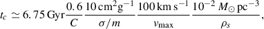
As we explain in Sect. 2 and show in Fig. 1, Yang et al. (2024) provide an analytical approximation for the time evolution of DM halos from initial NFW profiles to cored-collapsed halos. The halos are defined as
![Mathematical equation: $$ \begin{aligned} \rho _{\rm SIDM}(r) = \frac{1}{[(r/r_s^{\prime })^4+(r_c^{\prime }/r_s^{\prime })^4]^{1/4}}\frac{\rho ^{\prime }_s}{(1+r/r_s^{\prime })^2}, \end{aligned} $$](/articles/aa/full_html/2025/12/aa57040-25/aa57040-25-eq15.gif) (15)
(15)
where the free parameters ρ′s, r′s, and r′c depend on the age of the halo relative to the core-collapse timescale (Eq. (7)). Except when r′c = 0, this density presents an inner core of density
 (16)
(16)
When r′c → 0, Eq. (15) describes a NFW profile (Eq. (2)), which is what happens as tage → 0 since r′c → 0 as well. We note that rc′ parameterizes the core properties but is not the core radius (rc) that we employ in Eq. (6), which for the SIDM profile is implicitly defined from the expression
![Mathematical equation: $$ \begin{aligned} 2 r^{\prime }_c/r^{\prime }_s = (1+r_c/r_s^{\prime })^2\,[(r_c/r^{\prime }_s)^4+(r^{\prime }_c/r^{\prime }_s)^4]^{1/4}. \end{aligned} $$](/articles/aa/full_html/2025/12/aa57040-25/aa57040-25-eq17.gif) (17)
(17)
The parameters ρ′s, r′s, and r′c are worked out in Yang et al. (2024), normalized to the value that ρs′ and r′s have at tage = 0, i.e., when ρSIDM was a ρNFW profile of constants ρs and rs (Eq. (2)). Examples are given in Fig. 1a, where profiles before the core-formation time (tage < tc) are shown as dashed lines whereas profiles after core formation are shown using solid lines. Figure 1b shows the same profile as Fig. 1a with different normalization – they are normalized to the central density, Eq. (16), and to the core radius, Eq. (17). Figures 1c and 1c show how these two normalizing parameters vary with the age of the DM halo.
In order to obtain the core radius corresponding to a SIDM density profile with a given halo mass (Mh) and age, one has to assume the properties of the initial NFW halo and the SIDM cross section. For the initial NFW halo, we assumed the halo mass concentration relation from Sorini et al. (2025), but this selection does not significantly impact the results, as we analyze below.
As for the cross section, it varies with velocity (v) as
![Mathematical equation: $$ \begin{aligned} \frac{\sigma }{m}(v)=\frac{\sigma _0}{m}\,\frac{1+w_0^2/w_1^2}{1+\left[v-w_0\right]^2/w_1^2}, \end{aligned} $$](/articles/aa/full_html/2025/12/aa57040-25/aa57040-25-eq18.gif) (18)
(18)
which describes the existence of a resonance of width w1 at v = w0, as expected for some types of SIDM particles (see Tulin et al. 2013; Chu et al. 2019, 2020). More importantly, when w0 → 0 the resonance goes away and Eq. (18) describes the angular average cross section commonly used in the literature and appearing when the interaction between particles occurs through a Yukawa potential (Ibe & Yu 2010; Correa et al. 2022; Tam et al. 2023). The constant σ0/m parameterizes the cross section when v → 0. Examples of σ/m(v) from Eq. (18) are shown as the solid lines in Fig. 3, with the actual σ0/m, w0, and w1 given in the caption. The above assumptions allow the determination of the DM core radius as a function of halo mass, rc(Mh). In order to transform rc(Mh) to the observational plane stellar core radius (r★c) versus stellar mass (M★), two additional assumptions are needed, namely,
 (19)
(19)
and
 (20)
(20)
We consider δ ≃ 1 in Eq. (19) as an ansatz justified by the observation of some UFDs (Sánchez Almeida et al. 2024a), but it can be relaxed easily, as we explore below. The mapping in Eq. (20) is given in Appendix B, and it uses a recipe based on abundance matching for Mh ≳ 1010 M⊙ (Behroozi et al. 2013) and on numerical simulations for 108 M⊙ < Mh ≲ 1010 M⊙ (Kim et al. 2024). Its limitations are also explored below.
The stellar core versus stellar mass relation predicted by Eqs. (15)–(20) is shown in Fig. 4. Each line corresponds to the variation of r★c with M★ when the DM halo mass goes from 107 to 1014 M⊙ given a particular set of parameters. The type of line depends on whether the corresponding profile is in the core-formation phase (tage < tc; dashed line) or in the core-collapse phase (tage > tc; solid line) – note that the type of line sometimes changes as M★ varies. The parameters that define the cross sections are given in the inset (σ0/m, w0, and w1; see Eq. (18)), with the actual velocity dependence represented in Fig. 5 employing the same the color code used Fig. 4. The inset also includes tage, set to two values, tH/2 and tH/3. The blue line has been included to illustrate the impact on the core size of the existence of a resonance at ∼6 km s−1 (Fig. 5); it induces a sudden drop in r★c at around 103 M⊙ (Fig. 4). The figure also includes a number measurements of r★c versus M★ (the symbols) with the UFDs analyzed in this work appearing under the label SA+24 and represented with orange symbols. Figures 4 and 5 clearly shows that these UFD observations are reproduced when σ/m ∼ 0.1 cm2 g−1, if the galaxies were in the core-formation phase (the purple or magenta lines) or σ/m ∼ 300 cm2 g−1, if the galaxies were in the core-collapse phase (the lemon yellow or blue lines). These fact is in fair agreement with the range worked out in Sect. 2 and given in Eqs. (13) and (14). In addition to the UFDs, Fig. (4) displays a number of measurements represented by symbols. These measurements are labeled in the inset, with the equivalence between labels and references specified in Appendix C.
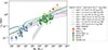 |
Fig. 4. Stellar core radius versus stellar mass as predicted by the simple model presented in Sect. 3. Each line shows the variation in r★c with M★ when the DM halo mass goes from 107 to 1014 M⊙. The type of line depends on whether the corresponding profile is in the core-formation phase (tage < tc; dashed line) or the core-collapse phase (tage > tc; solid line). The parameters that define the cross sections are given in the inset, with the actual velocity dependence represented in Fig. 5 with the same color code employed here. Observations of r★c versus M★ are represented as symbols, each one corresponding to an individual object. The measurements are labeled in the inset, with the UFDs analyzed in this work appearing under the label SA+24. The link between labels and references is specified in Appendix C. The figure also includes the theoretical expectations from stellar feedback on CDM halos from Lazar et al. (2020, the gray band and solid line). |
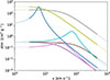 |
Fig. 5. Cross sections used to compute r★c(M★) in Fig. 4. The color code used here and in Fig. 4 is the same. The range of velocities highlighted with thicker lines corresponds to the range of effective velocities (Eq. (13)) when the halo masses go from 107 to 1014 M⊙, as used in Fig. 4. |
Figure 4 also includes the relation expected from stellar-feedback operating on CDM halos, as modeled by Lazar et al. (2020, the gray shaded area representing the scatter with the mean given by the solid line). Note the large discrepancy with observations at M★ < 106 M⊙, which just illustrates the result that stellar feedback does not produce cores in low mass CDM halos (see the arguments in Sect. 1). To transform the actual predictions to the observational plane, Eq. (19) with δ = 1 has been assumed. We note that the stellar feedback sub-grid physic implemented in the numerical simulation used by Lazar et al. (2020, FIRE2; Hopkins et al. 2018) is particularly effective at transferring supernova kinetic energy into the medium (e.g., Mitchell et al. 2020; Pandya et al. 2021) so that other alternative simulations will likely give even smaller cores, enhancing the tension with observations. When M★ > 106 M⊙, the figure suggests that stellar feedback has to be taken into account even if SIDM contributes to the formation of cores, since stellar feedback is present in real galaxies and it can potentially produce cores comparable in size to the observed ones.
Figure 6 provides the central density of the SIDM profiles used in Fig. 4. They are represented versus stellar core radius with the same color code employed in Figs. 4 and 5. The figure also shows a number of observed densities for UFD and dSph (dwarf Spheroidal) galaxies as collected by Silverman et al. (2023, their Fig. 10). The range of central densities observed in UFDs is well covered by the SIDM simulations, both in the core-formation and the core-collapse phase. The increase in the central density with decreasing radius found by Silverman et al. (2023) is consistent with the observation that the product ρDM(0) rc tends to be constant regardless of the DM halo mass, with a value of around 44 M⊙ pc−2 (Burkert 1995; Salucci & Burkert 2000; Kormendy & Freeman 2016; Sánchez Almeida 2025). This value is represented as the red dotted line in Fig. 6, assuming r★c ≃ rc. We note that the relation ρDM(0) rc ≃ const arises from the halo mass–concentration relation found in CDM numerical simulations, under the assumption that the observed cores result from the redistribution of mass from an initial NFW profile (see Sánchez Almeida 2025, and references therein). Consequently, any core density profile that originates from a NFW profile consistent with the mass–concentration relation and reproduces the observed core size will naturally match the observed central DM density. The models presented above and in Sect. 2 are of this kind, which explains why they also successfully recover the central densities.
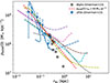 |
Fig. 6. Central density of the SIDM profiles used in Fig. 4 versus the stellar core radius. The color code employed in Figs. 4 and 5 is also used here. As in Fig. 4, the line is dashed or solid depending on whether the corresponding profile is in the core-formation phase (dashed line) or the core-collapse phase (solid line). The figure also includes a number of observed densities for UFDs and dSph collected by Silverman et al. (2023, their Fig. 10). The range of central densities observed in UFDs is covered by the SIDM simulations, both in the core-formation and the core-collapse phase. The increase in the central density with decreasing radius is consistent with the observations that the product central density times the core radius tends to be constant regardless of the DM halo mass, with a value of around 44 M⊙ pc−2. This trend is represented as the dotted red line, assuming rc ≃ r★c. |
Figure 7 explores the impact of the uncertainties in the free parameters that define the toy model. We modified the parameters for two models shown in Figs. 4–6. One of them has large cross section (lemon yellow line) while the other has low cross section (cyan line). They are represented in Fig. 7 with the same color as in Figs. 4–6. The M★ versus Mh relation (Eq. (20)) has a scatter worked out in Appendix B, and this scatter gives rise to the colored bands in Fig. 7 when the extreme M★(Mh) relations are used in the toy model. The impact of the concentration to halo mass relation is analyzed by considering another relation, by Correa et al. (2015, the dotted lines), often used in the literature. The uncertainty in the scaling between stellar and DM core radii (δ in Eq. (19)) just shifts down all the curves according to the value of δ. Neither this effect nor the change of age are included in Fig. 7. Changing the age is formally identical to changing the amplitude of the cross section since tage/tcc depends on the product tage σ0/m (Eqs. (3) and (7)). The effect is already illustrated in Fig. 4. All in all, the differences between r★c in the reference models and in all these alternatives are only around a factor of 2, which is smaller than the effect of changing the parameters that define the cross section (σ0/m, w0, and w1 in Eq. (18)) and smaller than the scatter among the observed galaxies (symbols in Fig. 4).
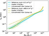 |
Fig. 7. Effect of the uncertainty in various parameters defining the toy model presented in Sect. 3. We use two reference models, one with a high cross section (lemon orange) and one with a low cross section (cyan). They are represented in Figs. 4–6 with the same color. These reference models are drawn with solid lines, whereas the shaded regions show the uncertainties in the stellar mass-to-halo mass relation. The dotted lines employ a different concentration-to-halo mass relation than the toy model. See the main text for further details. |
A few conclusions can be drawn from the inspection of Figs. 4–7: (1) The cross section required to explain the UFDs analyzed in Sect. 2 (the orange symbols) are in a range broadly consistent with Eqs. (11) and (14). (2) This toy model predicts an overall increase in the core size with increasing mass, which is in qualitative agreement with observations. Other models of DM, like Fuzzy DM, do not comply with this observational constraint (e.g., Burkert 2020; Benito et al. 2025). Stellar feedback qualitatively predicts the trend, but quantitatively falls too short to explain the stellar core sizes at M★ < 106 M⊙ (the gray shaded region in Fig. 4). (3) The uncertainty in the free parameters do not change the global trend of the dependence. Just produce an uncertainty in r★c within a factor of 2, which propagates into the value of σ0/m required to explain the observations. (4) The observed scatter is too large for the toy model, even when the uncertainties are considered. The origin of this diversity is unclear but may be due to the difference pathways followed by the different galaxies as advocated by Kamada et al. (2017) or Roberts et al. (2025).
4. Thermalization radius
Sections 2 and 3 show how the cores of UFDs can be produced by a small SIDM cross section, if the halos are in the core-formation phase, or by a large cross sections, if the halos are in the core-collapse phase (Fig. 2). Although the overall halo shape appears similar in the two phases (see Fig. 1b and Yang et al. 2024), the underlying physical processes differ. In the core-formation phase, only the core region is thermalized in the sense that only the DM particles within this inner core region have had enough time to collide and thermalize. Thus, the halo outskirts still reflect the NFW shape from which they originated. On the other hand, in the core-collapse phase, a significant part of the whole halo is thermalized, and its structure reflects the distribution expected in self-gravitating DM halos in thermodynamic equilibrium (see Sect. 1).
To work out the region of the halo that is thermalized in the two cases, we define the thermalization radius, rte, as the radius where
![Mathematical equation: $$ \begin{aligned} t_{\mathrm{age}}\simeq \frac{1}{\rho _{\rm NFW}(r_{te})\,v_{\rm NFW}(r_{te})}\,\frac{1}{[\sigma /m]\left(v_{\rm NFW}(r_{te})\right)}, \end{aligned} $$](/articles/aa/full_html/2025/12/aa57040-25/aa57040-25-eq21.gif) (21)
(21)
which follows from Eq. (1) with ρNFW(r) the NFW profile defined in Eq. (2) and vNFW(r) a representative relative velocity between particles in the halo, taken to be the velocity dispersion. Assuming isotropy for the velocity field, it is  times the radial velocity dispersion, which is approximately the circular velocity in NFW halos (e.g., Łokas & Mamon 2001). Thus,
 (22)
(22)
with
![Mathematical equation: $$ \begin{aligned} M_{\rm NFW}( < r)= 4\pi \rho _s r_s^3\,\left[\ln (1+r/r_s)-\frac{r/r_s}{1+r/r_s}\right]. \end{aligned} $$](/articles/aa/full_html/2025/12/aa57040-25/aa57040-25-eq24.gif) (23)
(23)
We note that the product ρNFW(r) vNFW(r) is a monotonically decreasing function of r so that, according to Eq. (21), the halos are expected to be thermalized inside-out as tage increases. Moreover, since ρNFW(r) vNFW(r)∝r−1/2 when r → 0, Eq. (21) always has solution for any tage provided σ/m.
The cross section to be used in our estimate are the same used everywhere else in the work (Eq. (18)). Therefore, once σ0/m, w0, w1 and mass of the DM halo are set, the thread of assumptions and arguments made in Sect. 3 allows us to compute rte = rte(M★). This function is shown in Fig. 8 for the two extreme cross sections employed in Fig. 7; σ0/m = 0.3 cm2 g−1 and 400 cm2 g−1. When the cross section is small (cyan lines), the thermalization radius (dashed line) and the stellar core radius derived in Sect. 3 (solid line) are similar, in particular, rte ∼ r★c in the region of interest for UFDs where M★ < 106 M⊙. On the contrary, for large cross sections (lemon yellow lines) the thermalization radius is orders of magnitude larger than the stellar core radius (rte ≫ r★c); rte is even larger than the characteristic radius of the NFW (rs), although does not reaches the virial radius (rvir). Both rs and rvir, which are the same for the two cross sections, are shown in Fig. 8 as the dotted red line and the dotted dashed red line, respectively.
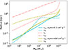 |
Fig. 8. Comparison between the thermalization radius (rte; Eq. (21)) and the stellar core radius (r★c). When the cross section is small (σ0/m = 0.3 cm2 g−1; the cyan lines), then rte and rc are similar, particularly in the region of interest for UFDs, where M★ < 106 M⊙. On the contrary, rte ≫ r★c for large cross sections (σ0/m = 400 cm2 g−1; the lemon yellow lines). For reference, the characteristic radius of the original NFW (rs; the dotted red line) and the virial radius (rvir; the dotted-dashed red line) are included. |
5. Conclusions
Sánchez Almeida et al. (2024a) argued that the stellar cores observed in UFDs reveal underlying DM cores that cannot be created by stellar feedback on collision-less CDM halos. Assuming this is true, we investigated the constraints imposed by such cores if they arise from self-interactions between DM particles (i.e., from SIDM).
The scaling relation from Outmezguine et al. (2023) is used in Sect. 2 to work out the SIDM cross sections able to generate the cores. They are given in Eq. (11) for the typical velocity in Eq. (14) (see the red symbol with error bars in Fig. 3). The observed core sizes can be produced by SIDM halos that are in the core-formation phase (implying a low σ/m) or in the core-collapse phase (implying a high σ/m). The range of possible σ/m values is relatively wide and aligns with those reported in the literature and summarized in Fig. 3. Several conclusions can be drawn from the figure: since stellar feedback cannot account for the presence of cores in these systems, UFDs provide a clean anchor point for constraining the velocity-dependent cross section at low velocities. This is in contrast to more luminous dwarf galaxies, where core formation can be significantly influenced by baryonic feedback. The observed scatter in cross sections for different galaxies may arise from known but uncorrected biases (such as neglecting baryonic effects) as well as from less well-understood systematics, including variations in the definition of velocity and cross section employed by different authors. It may also be real and reflect an intrinsic diversity in galaxy properties.
The exercise carried out in Sect. 2 is complemented in Sect. 3 with a simple model for the expected dependence on stellar mass of the stellar core radius produced by SIDM. The advantage of modeling stellar mass and stellar core radius is that both quantities are relatively easy to observe and should be closely related under SIDM scenarios. Using the time evolution of core SIDM profiles by Yang et al. (2024), we were able to predict core sizes given galaxy masses and ages. According to this model, the stellar cores in UFDs require cross sections similar to the ones inferred in Sect. 2 (see Figs. 4 and 5). Moreover, the modeling reveals a trend of increasing stellar core radius with stellar mass, consistent with the behavior observed in more massive dwarf galaxies. DM of a different nature, such as fuzzy DM, does not satisfy this observational constraint (e.g., Burkert 2020; Benito et al. 2025). Stellar feedback qualitatively predicts the trend but quantitatively falls too short to explain the stellar core sizes at M★ < 106 M⊙ (see the gray shaded region in Fig. 4). We examined the sensitivity of the model predictions to variations in its free parameters, finding no significant impact on the predicted global trends. Variations in the free parameters lead to variations in the stellar core radii by up to a factor of 2, which are smaller than the effect of changing the parameters that define the cross sections and also smaller than the scatter among the observed galaxies (see Fig. 4). The observed scatter is too large to be accounted for by the toy model, even when the uncertainties are considered. As already mentioned, the origin of this diversity (artificial or real) remains to be explained. If real, it may be due to differences in the star-formation histories of the different galaxies (e.g., Kamada et al. 2017; Roberts et al. 2025).
We find that the central DM densities of the SIDM halos in the model are consistent with the observed values, which increase with decreasing core size to yield a ρDM(0) rc that is approximately constant at around 44 M⊙ pc−2 (see Fig. 6). The constancy arises from the halo mass–concentration relation found in CDM numerical simulations, under the assumption that the observed cores result from the redistribution of mass from an initial NFW profile (see Sánchez Almeida 2025, and references therein). Consequently, any core model that originates from an NFW profile consistent with the mass–concentration relation and reproduces the observed core size will naturally match the observed central DM density. The model presented in Sect. 3 is of this kind, which explains why it successfully recovers the central densities.
As mentioned above, cross sections consistent with the observed cores can be found for both SIDM halos in the process of forming a core and halos in the core-collapse phase. While both solutions are possible, the physics giving rise to the SIDM distribution in the halo is different. Only the DM particles forming the core have interacted during the core-formation phase, whereas the rest maintain the original distribution from collision-less CDM halos. In core-collapse, however, the whole halo is in thermodynamic equilibrium. Section 4 demonstrates that, if the DM dark halos in UFDs are core-collapsing, the thermalization radii needed to account for the observed cores are quite large, on the order of 1 kpc for galaxies with M★ < 106 M⊙ (see Fig. 8). Thus, if the DM is self-interacting and has a large cross section within the range found in our work (∼200 cm2 g−1; Eq. (11)), one would expect that the self-interactions smear DM substructure on sub-kiloparsec scales in massive galaxies. Such smearing is expected to manifest in SIDM simulations. Unfortunately, there are very few cosmological simulations that include large SIDM cross sections, and the existing ones (Turner et al. 2021; Correa et al. 2022; Nadler et al. 2023) are focused on the properties of satellites around Milky Way-like galaxies rather than on the analysis of the DM substructure resulting from such extreme SIDM properties. New tailored simulations that accurately trace scales of 1 kpc and smaller are required to address this problem. Such simulations are needed to explore possible observational effects (e.g., the impact of SIDM on the expected galaxy–galaxy lensing signal; Dutra et al. 2025). In addition, these large cross sections may also have some impact on the matter-power spectrum that provides the initial conditions for the galaxies to form and evolve (e.g., Egana-Ugrinovic et al. 2021; Garani et al. 2022), an uncertain issue to be tackled systematically in the future (e.g., Nadler et al. 2025).
The appendices contain several byproducts of our analysis. A stellar-to-halo mass relation, which goes seamlessly from 108 to 1015 M⊙, is worked out in Appendix B. Appendix A provides a literature review of the cross sections proposed to explain observations going from gravitational lensing to galaxy cluster collisions, including the modeling of dwarf galaxies. Appendix D shows how the stellar distribution observed in UFDs is well reproduced by the cored SIDM halo shape employed in this work (ρSIDM, defined in Eq. (15)).
Acknowledgments
I am grateful to Ignacio Trujillo, Claudio Dalla Vecchia, Ethan Nadler, Hai-Bo Yu, Manoj Kaplinghat, Pavel Mancera Piña, Filippo Fraternali, and Jorge Peñarrubia for their valuable comments and discussions on specific aspects of this work. Thanks are also due to Scott Carlsten for providing some of the observational data used in Fig. 4, and to an anonymous referee for suggesting clarifications that strengthened the arguments in the paper. The research is partly funded through grant PID2022-136598NB-C31 (ESTALLIDOS 8) by the Spanish Ministry of Science and Innovation (MCIN/AEI/10.13039/501100011033) and “ERDF A way of making Europe”. The author has been supported by the European Union through the grant “UNDARK” of the Widening participation and spreading excellence programe (project number 101159929).
References
- Adhikari, S., Banerjee, A., Boddy, K. K., et al. 2022, Rev. Mod. Phys., submitted [arXiv:2207.10638] [Google Scholar]
- Adhikari, S., Banerjee, A., Jain, B., Shin, T.-H., & Zhong, Y.-M. 2025, ApJ, 983, 50 [Google Scholar]
- An, J. H., & Evans, N. W. 2006, ApJ, 642, 752 [NASA ADS] [CrossRef] [Google Scholar]
- Ando, S., Hayashi, K., Horigome, S., Ibe, M., & Shirai, S. 2025, arXiv e-prints [arXiv:2503.13650] [Google Scholar]
- Andrade, K. E., Fuson, J., Gad-Nasr, S., et al. 2022, MNRAS, 510, 54 [Google Scholar]
- Argüelles, C. R., Becerra-Vergara, E. A., Rueda, J. A., & Ruffini, R. 2023, Universe, 9, 197 [CrossRef] [Google Scholar]
- Balberg, S., Shapiro, S. L., & Inagaki, S. 2002, ApJ, 568, 475 [CrossRef] [Google Scholar]
- Battaglia, G., & Nipoti, C. 2022, Nat. Astron., 6, 659 [NASA ADS] [CrossRef] [Google Scholar]
- Battaglia, G., Tolstoy, E., Helmi, A., et al. 2006, A&A, 459, 423 [NASA ADS] [CrossRef] [EDP Sciences] [Google Scholar]
- Behroozi, P. S., Wechsler, R. H., & Conroy, C. 2013, ApJ, 770, 57 [NASA ADS] [CrossRef] [Google Scholar]
- Behroozi, P., Wechsler, R. H., Hearin, A. P., & Conroy, C. 2019, MNRAS, 488, 3143 [NASA ADS] [CrossRef] [Google Scholar]
- Benito, M., Hütsi, G., Müürsepp, K., et al. 2025, Phys. Dark Universe, 49, 102010 [Google Scholar]
- Binney, J., & Tremaine, S. 2008, Galactic Dynamics: Second Edition (Princeton University Press) [Google Scholar]
- Bode, P., Ostriker, J. P., & Turok, N. 2001, ApJ, 556, 93 [Google Scholar]
- Bradač, M., Allen, S. W., Treu, T., et al. 2008, ApJ, 687, 959 [CrossRef] [Google Scholar]
- Brown, S. T., McCarthy, I. G., Diemer, B., et al. 2020, MNRAS, 495, 4994 [NASA ADS] [CrossRef] [Google Scholar]
- Buckley, M. R., & Fox, P. J. 2010, Phys. Rev. D, 81, 083522 [CrossRef] [Google Scholar]
- Bullock, J. S., & Boylan-Kolchin, M. 2017, ARA&A, 55, 343 [Google Scholar]
- Burkert, A. 1995, ApJ, 447, L25 [NASA ADS] [Google Scholar]
- Burkert, A. 2020, ApJ, 904, 161 [NASA ADS] [CrossRef] [Google Scholar]
- Carlsten, S. G., Greene, J. E., Beaton, R. L., Danieli, S., & Greco, J. P. 2022, ApJ, 933, 47 [CrossRef] [Google Scholar]
- Chu, X., & Garcia-Cely, C. 2018, JCAP, 2018, 013 [Google Scholar]
- Chu, X., Garcia-Cely, C., & Murayama, H. 2019, Phys. Rev. Lett., 122, 071103 [Google Scholar]
- Chu, X., Garcia-Cely, C., & Murayama, H. 2020, JCAP, 2020, 043 [CrossRef] [Google Scholar]
- Correa, C. A. 2021, MNRAS, 503, 920 [NASA ADS] [CrossRef] [Google Scholar]
- Correa, C. A., Wyithe, J. S. B., Schaye, J., & Duffy, A. R. 2015, MNRAS, 452, 1217 [CrossRef] [Google Scholar]
- Correa, C. A., Schaller, M., Ploeckinger, S., et al. 2022, MNRAS, 517, 3045 [NASA ADS] [CrossRef] [Google Scholar]
- de Boer, T. J. L., & Fraser, M. 2016, A&A, 590, A35 [NASA ADS] [CrossRef] [EDP Sciences] [Google Scholar]
- Del Popolo, A., & Le Delliou, M. 2017, Galaxies, 5, 17 [Google Scholar]
- Delgado, V., & Muñoz Mateo, A. 2023, MNRAS, 518, 4064 [Google Scholar]
- Delos, M. S., & White, S. D. M. 2023, MNRAS, 518, 3509 [Google Scholar]
- Donato, F., Gentile, G., Salucci, P., et al. 2009, MNRAS, 397, 1169 [Google Scholar]
- Drlica-Wagner, A., Bechtol, K., Rykoff, E. S., et al. 2015, ApJ, 813, 109 [Google Scholar]
- Dutra, I., Natarajan, P., & Gilman, D. 2025, ApJ, 978, 38 [Google Scholar]
- Eckert, D., Ettori, S., Robertson, A., et al. 2022, A&A, 666, A41 [NASA ADS] [CrossRef] [EDP Sciences] [Google Scholar]
- Efstathiou, G. 2025, Philos. Trans. R. Soc. Lond. Ser. A, 383, 20240022 [Google Scholar]
- Egana-Ugrinovic, D., Essig, R., Gift, D., & LoVerde, M. 2021, JCAP, 2021, 013 [CrossRef] [Google Scholar]
- Elbert, O. D., Bullock, J. S., Garrison-Kimmel, S., et al. 2015, MNRAS, 453, 29 [NASA ADS] [CrossRef] [Google Scholar]
- Elbert, O. D., Bullock, J. S., Kaplinghat, M., et al. 2018, ApJ, 853, 109 [CrossRef] [Google Scholar]
- Feng, J. L., Kaplinghat, M., Tu, H., & Yu, H.-B. 2009, JCAP, 2009, 004 [CrossRef] [Google Scholar]
- Ferragamo, A., Barrena, R., Rubiño-Martín, J. A., et al. 2021, A&A, 655, A115 [NASA ADS] [CrossRef] [EDP Sciences] [Google Scholar]
- Garani, R., Redi, M., & Tesi, A. 2022, JCAP, 2022, 012 [CrossRef] [Google Scholar]
- Gilman, D., Zhong, Y.-M., & Bovy, J. 2023, Phys. Rev. D, 107, 103008 [NASA ADS] [CrossRef] [Google Scholar]
- Gopika, K., & Desai, S. 2023, Phys. Dark Universe, 42, 101291 [Google Scholar]
- Governato, F., Brook, C., Mayer, L., et al. 2010, Nature, 463, 203 [NASA ADS] [CrossRef] [Google Scholar]
- Harvey, D., Massey, R., Kitching, T., Taylor, A., & Tittley, E. 2015, Science, 347, 1462 [Google Scholar]
- Harvey, D., Robertson, A., Massey, R., & McCarthy, I. G. 2019, MNRAS, 488, 1572 [NASA ADS] [CrossRef] [Google Scholar]
- Hopkins, P. F., Wetzel, A., Kereš, D., et al. 2018, MNRAS, 480, 800 [NASA ADS] [CrossRef] [Google Scholar]
- Ibe, M., & Yu, H.-B. 2010, Phys. Lett. B, 692, 70 [Google Scholar]
- Indjin, M., Liu, I. K., Proukakis, N. P., & Rigopoulos, G. 2025, arXiv e-prints [arXiv:2502.04838] [Google Scholar]
- Into, T., & Portinari, L. 2013, MNRAS, 430, 2715 [Google Scholar]
- Jiang, F., Jiang, Z., Zheng, H., et al. 2025, ApJL, submitted [arXiv:2503.23710] [Google Scholar]
- Kahlhoefer, F., Schmidt-Hoberg, K., Kummer, J., & Sarkar, S. 2015, MNRAS, 452, L54 [CrossRef] [Google Scholar]
- Kamada, A., Kaplinghat, M., Pace, A. B., & Yu, H.-B. 2017, Phys. Rev. Lett., 119, 111102 [Google Scholar]
- Kaplinghat, M., Tulin, S., & Yu, H.-B. 2016, Phys. Rev. Lett., 116, 041302 [NASA ADS] [CrossRef] [Google Scholar]
- Kaplinghat, M., Valli, M., & Yu, H.-B. 2019, MNRAS, 490, 231 [NASA ADS] [CrossRef] [Google Scholar]
- Kim, S. Y., Read, J. I., Rey, M. P., et al. 2024, MNRAS, submitted [arXiv:2408.15214] [Google Scholar]
- Kormendy, J., & Freeman, K. C. 2016, ApJ, 817, 84 [NASA ADS] [CrossRef] [Google Scholar]
- Lazar, A., Bullock, J. S., Boylan-Kolchin, M., et al. 2020, MNRAS, 497, 2393 [NASA ADS] [CrossRef] [Google Scholar]
- Leung, G. Y. C., Leaman, R., van de Ven, G., & Battaglia, G. 2020, MNRAS, 493, 320 [Google Scholar]
- Leung, G. Y. C., Leaman, R., Battaglia, G., et al. 2021, MNRAS, 500, 410 [Google Scholar]
- Loeb, A., & Weiner, N. 2011, Phys. Rev. Lett., 106, 171302 [NASA ADS] [CrossRef] [Google Scholar]
- Łokas, E. L., & Mamon, G. A. 2001, MNRAS, 321, 155 [CrossRef] [Google Scholar]
- Lu, Y., Mo, H. J., Katz, N., & Weinberg, M. D. 2006, MNRAS, 368, 1931 [NASA ADS] [CrossRef] [Google Scholar]
- Mancera Piña, P. E., Golini, G., Trujillo, I., & Montes, M. 2024, A&A, 689, A344 [NASA ADS] [CrossRef] [EDP Sciences] [Google Scholar]
- Martin, N. F., de Jong, J. T. A., & Rix, H.-W. 2008, ApJ, 684, 1075 [NASA ADS] [CrossRef] [Google Scholar]
- Massey, R., Williams, L., Smit, R., et al. 2015, MNRAS, 449, 3393 [Google Scholar]
- Mitchell, P. D., Schaye, J., Bower, R. G., & Crain, R. A. 2020, MNRAS, 494, 3971 [Google Scholar]
- Montes, M., Trujillo, I., Karunakaran, A., et al. 2024, A&A, 681, A15 [NASA ADS] [CrossRef] [EDP Sciences] [Google Scholar]
- Muñoz, R. R., Côté, P., Santana, F. A., et al. 2018, ApJ, 860, 66 [CrossRef] [Google Scholar]
- Nadler, E. O., Yang, D., & Yu, H.-B. 2023, ApJ, 958, L39 [NASA ADS] [CrossRef] [Google Scholar]
- Nadler, E. O., An, R., Yang, D., et al. 2025, ApJ, 986, 129 [Google Scholar]
- Navarro, J. F., Frenk, C. S., & White, S. D. M. 1997, ApJ, 490, 493 [Google Scholar]
- Outmezguine, N. J., Boddy, K. K., Gad-Nasr, S., Kaplinghat, M., & Sagunski, L. 2023, MNRAS, 523, 4786 [NASA ADS] [CrossRef] [Google Scholar]
- Pandya, V., Fielding, D. B., Anglés-Alcázar, D., et al. 2021, MNRAS, 508, 2979 [NASA ADS] [CrossRef] [Google Scholar]
- Peebles, P. J. E. 2021, arXiv e-prints [arXiv:2106.02672] [Google Scholar]
- Peñarrubia, J., Pontzen, A., Walker, M. G., & Koposov, S. E. 2012, ApJ, 759, L42 [CrossRef] [Google Scholar]
- Peter, A. H. G., Rocha, M., Bullock, J. S., & Kaplinghat, M. 2013, MNRAS, 430, 105 [Google Scholar]
- Plastino, A. R., & Plastino, A. 1993, Phys. Lett. A, 174, 384 [NASA ADS] [CrossRef] [Google Scholar]
- Pontzen, A., & Governato, F. 2012, MNRAS, 421, 3464 [NASA ADS] [CrossRef] [Google Scholar]
- Randall, S. W., Markevitch, M., Clowe, D., Gonzalez, A. H., & Bradač, M. 2008, ApJ, 679, 1173 [NASA ADS] [CrossRef] [Google Scholar]
- Read, J. I., Walker, M. G., & Steger, P. 2018, MNRAS, 481, 860 [NASA ADS] [CrossRef] [Google Scholar]
- Richstein, H., Kallivayalil, N., Simon, J. D., et al. 2024, ApJ, 967, 72 [NASA ADS] [CrossRef] [Google Scholar]
- Roberts, M. G., Kaplinghat, M., Valli, M., & Yu, H.-B. 2025, Phys. Rev. D, 111, 103041 [Google Scholar]
- Robertson, A., Harvey, D., Massey, R., et al. 2019, MNRAS, 488, 3646 [NASA ADS] [CrossRef] [Google Scholar]
- Sagunski, L., Gad-Nasr, S., Colquhoun, B., Robertson, A., & Tulin, S. 2021, JCAP, 2021, 024 [CrossRef] [Google Scholar]
- Salucci, P. 2019, A&ARv, 27, 2 [NASA ADS] [CrossRef] [Google Scholar]
- Salucci, P., & Burkert, A. 2000, ApJ, 537, L9 [NASA ADS] [CrossRef] [Google Scholar]
- Sánchez Almeida, J. 2022, Universe, 8, 214 [CrossRef] [Google Scholar]
- Sánchez Almeida, J. 2025, Galaxies, 13, 6 [Google Scholar]
- Sánchez Almeida, J., Trujillo, I., & Plastino, A. R. 2020, A&A, 642, L14 [NASA ADS] [CrossRef] [EDP Sciences] [Google Scholar]
- Sánchez Almeida, J., Plastino, A. R., & Trujillo, I. 2023, ApJ, 954, 153 [CrossRef] [Google Scholar]
- Sánchez Almeida, J., Trujillo, I., & Plastino, A. R. 2024a, ApJ, 973, L15 [Google Scholar]
- Sánchez Almeida, J., Plastino, A. R., & Trujillo, I. 2024b, A&A, 690, A151 [NASA ADS] [CrossRef] [EDP Sciences] [Google Scholar]
- Sánchez Almeida, J., Trujillo, I., Montes, M., & Plastino, A. R. 2025, A&A, 694, A283 [NASA ADS] [CrossRef] [EDP Sciences] [Google Scholar]
- Sarkar, S. 2018, Nat. Astron., 2, 856 [Google Scholar]
- Schive, H.-Y., Chiueh, T., & Broadhurst, T. 2014, Nat. Phys., 10, 496 [NASA ADS] [CrossRef] [Google Scholar]
- Shi, Y., Zhang, Z.-Y., Wang, J., et al. 2021, ApJ, 909, 20 [NASA ADS] [CrossRef] [Google Scholar]
- Shin, T., Jain, B., Adhikari, S., et al. 2021, MNRAS, 507, 5758 [NASA ADS] [CrossRef] [Google Scholar]
- Silk, J. 2017, in 14th International Symposium on Nuclei in the Cosmos (NIC2016), eds. S. Kubono, T. Kajino, S. Nishimura, et al., 010101 [Google Scholar]
- Silverman, M., Bullock, J. S., Kaplinghat, M., Robles, V. H., & Valli, M. 2023, MNRAS, 518, 2418 [Google Scholar]
- Simon, J. D. 2019, ARA&A, 57, 375 [NASA ADS] [CrossRef] [Google Scholar]
- Sorini, D., Bose, S., Pakmor, R., et al. 2025, MNRAS, 536, 728 [Google Scholar]
- Spergel, D. N., & Steinhardt, P. J. 2000, Phys. Rev. Lett., 84, 3760 [NASA ADS] [CrossRef] [Google Scholar]
- Tam, S.-I., Umetsu, K., Robertson, A., & McCarthy, I. G. 2023, ApJ, 953, 169 [CrossRef] [Google Scholar]
- Tasitsiomi, A., Kravtsov, A. V., Gottlöber, S., & Klypin, A. A. 2004, ApJ, 607, 125 [NASA ADS] [CrossRef] [Google Scholar]
- Tian, Y., Umetsu, K., Ko, C.-M., Donahue, M., & Chiu, I. N. 2020, ApJ, 896, 70 [NASA ADS] [CrossRef] [Google Scholar]
- Tollet, E., Macciò, A. V., Dutton, A. A., et al. 2016, MNRAS, 456, 3542 [CrossRef] [Google Scholar]
- Tulin, S., & Yu, H.-B. 2018, Phys. Rep., 730, 1 [Google Scholar]
- Tulin, S., Yu, H.-B., & Zurek, K. M. 2013, Phys. Rev. Lett., 110, 111301 [Google Scholar]
- Turner, H. C., Lovell, M. R., Zavala, J., & Vogelsberger, M. 2021, MNRAS, 505, 5327 [CrossRef] [Google Scholar]
- Vega-Ferrero, J., Dana, J. M., Diego, J. M., et al. 2021, MNRAS, 500, 247 [Google Scholar]
- Wandelt, B. D., Dave, R., Farrar, G. R., et al. 2001, in Sources and Detection of Dark Matter and Dark Energy in the Universe, ed. D. B. Cline, 263 [Google Scholar]
- Yang, D., & Yu, H.-B. 2022, JCAP, 2022, 077 [CrossRef] [Google Scholar]
- Yang, D., Nadler, E. O., Yu, H.-B., & Zhong, Y.-M. 2024, JCAP, 2024, 032 [Google Scholar]
Appendix A: Comments on the references represented in Fig. 3.
Figure 3 was meant to collect a representative set of σ/m values found in the literature. The references were selected from the ∼ 700 papers citing the seminal work where Randall et al. (2008) set an upper limit on σ/m from the lack of separation between DM and stars in the Bullet Cluster. The sources are quite diverse and there is no general rule on how σ/m and velocity are inferred from the observational data. Thus, a significant part of the scatter in Fig. 3 is due to the different analyses of the observational data leading to average cross sections and characteristic velocities. This appendix provides the equivalence between the label given the inset of Fig. 3 and the actual reference, and it also outlines the different meaning for SIDM cross section and typical velocity employed in different works.
- Randall+08: Randall et al. (2008) is the reference work setting an upper limit after the lack of significant separation between stars (from galaxies) and DM (from lensing) in the Bullet Cluster. It is based on comparison with numerical simulations made at the date of publication.
- SA+24: This work. The limits are worked out in Sect. 2, Eqs. (12) and (14), to represent the constraints imposed by the UFDs compiled by Richstein et al. (2024) after the analysis carried out by Sánchez Almeida et al. (2024a).
- Jiang+25: Jiang et al. (2025) explain the formation of Intermediate-Mass Black Holes (IMBHs) from the core collapse of SIDM halos. They successfully reproduce the observed little red dot mass function with σ0/m ∼ 30 cm2 g−1, w0 = 0 km s−1, and w1 ∼ 80 km s−1 (Eq. [18]).
- Robertson+19: Comparing Einstein radii of SIDM simulated galaxy clusters with those observed in the CLASH survey, Robertson et al. (2019) set the upper limit used in the figure.
- Kahl.+15: Explaining with SIDM the separation between stars and DM of a galaxy falling into a galaxy cluster (Massey et al. 2015), Kahlhoefer et al. (2015) need the cross section shown in the figure. The authors also estimate the large velocity of the DM of the falling galaxy relative to the ambient medium.
- Peter+13: Cross section based on comparing the shape of the lensing potentials with the X-ray isophotes of the massive elliptical NGC 720. According to Peter et al. (2013), the observations allow for the cross section employed in the figure. The velocity comes from the virial mass of the galaxy.
- Read+18: The high central density of Draco enabled Read et al. (2018) to set an upper limit on the SIDM cross section. The velocity was taken as the observed velocity dispersion along the line of sight.
- Harvey+19: In SIDM halos, the position of brightest cluster galaxy in a galaxy cluster may be offset with respect to the DM distribution. Harvey et al. (2019) use SIDM cosmological simulations with stellar feedback to set the upper limit to the cross section in Fig. 3. It is based on 10 observed clusters. The velocity comes from the dynamical mass of the clusters.
- Ekert+22: From simulations of galaxy clusters, Eckert et al. (2022) work out a relation between the parameter α of the Einasto profile and the SIDM cross section. The profile observed in 12 massive clusters is consistent with CDM, which allowed them to set the upper limit used in the figure. They also provide the typical relative velocity of the DM particles.
- Gilman+23: Gilman et al. (2023) constrain resonant DM self-interactions with strong gravitational lenses. The diagnostics is based on whether or not the DM halos in the lens have core-collapsed. They set a fairly large upper limit at low velocities.
- Ebert+18: From the comparison of SIDM cosmological numerical simulations with the brightest central galaxy of A2667, Elbert et al. (2018) set the upper limit at large relative velocity included in the figure.
- Adhi.+25: Using the weak-lensing measurements reported by Shin et al. (2021), cosmological N-body simulations, and semi-analytical fluid simulations, Adhikari et al. (2025) set the upper limit shown in the figure. Characteristic velocities are not given. Those in the figure come from the cluster halo masses turned into velocity through Eq. (1) in Ferragamo et al. (2021).
- Gopika+24: Following the singular approach of Eckert et al. (2022), Gopika & Desai (2023) analyze the X-ray DM profiles of 11 relaxed galaxy groups. They give a cross section and upper limits for relative velocities between 200 and 700 km s−1.
- Tam+23: Tam et al. (2023) compare the radial acceleration relation observed in 20 high-mass galaxy clusters by Tian et al. (2020) with SIDM cosmological hydrodynamical simulations. They discard σ/m larger than the limit used in the figure. No characteristic velocity is given but it was estimated from the DM halo mass as we did for Adhikari et al. (2025).
- Andrade+22: Andrade et al. (2022) analyze strongly lensed images of 8 galaxy clusters to measure their DM density profiles. Using their DM central density, they assign the cross section used in the figure, which can also be understood as an upper limit. A characteristic velocity is given in the paper.
- Shi+21: Shi et al. (2021) analyze the rotation of the irregular galaxy AGC 242019, which happens to be consistent with a cuspy NFW DM density profile. This information is used to set the upper limit for the cross section used in the figure. The characteristic velocity is taken form the circular velocity in their Table 2.
- Correa 21: Correa (2021) models the anticorrelation between the central DM densities of dSph satellites of the Milky Way and their pericenter distances observed by Kaplinghat et al. (2019). Using the gravo-thermal fluid formalism to model the subhalo density profiles, the correlation can be reproduced with the values of cross section and velocity employed in the figure.
- Kap.+16: Seminal paper by Kaplinghat et al. (2016) where the DM cores of objects going from dwarf galaxies to clusters of galaxies are interpreted in terms of SIDM. The contribution of baryon feedback is ignored.
- Vega+21: Vega-Ferrero et al. (2021) model the morphology of giant arcs in galaxy clusters using N-body and smoothed-particle hydrodynamics simulations assuming both CDM and SIDM. They conclude that it is not possible to rule out a SIDM cross section as the one defining the upper limit represented in the figure. The velocities is inferred from the DM halo mass with the recipe used for Adhikari et al. (2025).
- Sag.+21: Sagunski et al. (2021) use both lensing signals and stellar dispersions to model eight galaxy groups and seven massive galaxy clusters. They provide two points in our figure, one for groups and another for clusters. Characteristic velocities are estimated from halo masses as done for Adhikari et al. (2025).
- Harvey+15: Harvey et al. (2015) measure the separation between the DM structure and the galaxies in around 30 colliding galaxy clusters. The DM is located via gravitational lensing whereas imaging and X-rays provide the stars and the gas. The lack of separation between DM and stars allowed them to set the upper limit shown in the figure. Velocities come from halo masses as done for Adhikari et al. (2025).
- Bradac+08: Bradač et al. (2008) carry out a work similar to the one for the Bullet cluster by Randall et al. (2008). They analyze a recently identified massive merging galaxy cluster, MACS J0025.4-1222. Lensing provides the DM distribution whereas optical data and X-ray render the distribution of stars and gas, respectively. The total mass distribution is offset from the hot X-ray-emitting gas but aligned with the distribution of galaxies. This is used to set an upper limit to the SIDM cross section used in the figure. Typical velocities are provided by the authors.
- Leung+21: Leung et al. (2021) analyze the isolated dwarf irregular galaxy WLM. Photometric data and the HI rotation curve can be reproduced with the SIDM cross section used in the figure. Its value together with the characteristic relative velocity are taken from their Fig. 8.
- Leung+20: Leung et al. (2020) compare the DM core size of the Fornax dwarf galaxy finding it to be large for CDM but consistent with SIDM, with the cross section used in the figure. As characteristic velocity, Fig. 3 uses the velocity dispersion of the stars along the line of sight.
- Mancera+24: Mancera Piña et al. (2024) fit the rotation curve of the gas-rich ultra-diffuse dwarf AGC 114905 assuming different models of DM, including SIDM. Two different SIDM models fit equality well. Figure 3 uses the cross sections at vmax, which follow from the relation hypothesized by Nadler et al. (2023).
- Ando+25: Ando et al. (2025) fit the radial distribution of velocity dispersions in a number of UFDs and dSph galaxies. Assuming a number of priors for the galaxy properties, they carry out a Bayesian fit that provides a range SIDM cross sections that are favored or discarded. The ones corresponding to velocity independent cross sections (bottom right panels in their Figs. 3 and 4) are represented in Fig. 3. The used velocity is the typical observed velocity dispersion provided in the manuscript.
Appendix B: Stellar mass–halo mass relation
The analysis carried out in Sects. 3 and 4 requires using a stellar mass (M★) to halo mass (Mh) relation since the collisions between DM particles depend on Mh, whereas M★ is the true observable. For massive galaxies, log(Mh/M⊙)≳10.5, we use the well-known relation by Behroozi et al. (2013), which is derived from observations through abundance matching. This range of masses does not include the low-mass regime of interest. Kim et al. (2024) provide this mass regime based on numerical simulations that goes all the way down to log(Mh/M⊙)∼8. Thus, we worked out a piecewise M★ = M★(Mh) relation coinciding with Kim et al. (2024) at low mass (the orange line in Fig. B.1) and with Behroozi et al. (2013) at high mass (the blue line in Fig. B.1). A polynomial seamlessly joins them at log(Mh/M⊙) = 10.976. The full relation, shown as a black dashed line in Fig. B.1, is
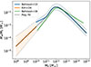 |
Fig. B.1. Piecewise M★ = M★(Mh) used in Sects. 3 and 4 (the dashed lines; Eqs. [B.1] and [B.2]). A polynomial seamlessly joins the relationships worked out by Behroozi et al. (2013, high mass) and by Kim et al. (2024, low mass). For additional details, see Appendix B. |
 (B.1)
(B.1)
with x = (log Mh − 12.3)/1.3,


where all the masses are in M⊙. Error bars for this function are also estimated by joining those provided by Kim et al. (2024, the orange shaded region in Fig. B.1) with those by Behroozi et al. (2013, the blue shaded region in Fig. B.1),
 (B.2)
(B.2)
where ±Δlog M★ are shown as dashed-dotted gray lines in Fig. B.1. These error bars are quite generous and include other M★(Mh) estimates (e.g., Behroozi et al. 2019, represented in Fig. B.1 as a green line).
Appendix C: Details of the observations represented in Fig. 4
The appendix gives the references for the observations plotted in Fig. 4. It also explains how the core radii used originally were matched to the definition employed in the work (Eq. [6]).
- The core radii of the UFDs from Richstein et al. (2024) are computed from the fits by Sánchez Almeida et al. (2024b) to the stellar surface density Σ(R), and assuming that R★c ≃ r★c with Σ(R★c) = Σ(0)/2, an approximation that holds for Schuster-Plummer profiles (see Sánchez Almeida 2022, 2025).
- The galaxy Nube, discovered by Montes et al. (2024), is particularly large for its mass. It has a conspicuously large core. The discoverers give its stellar mass, 4 × 10⁸ M⊙, and its projected core radius, R★c ≃ 6.6 kpc. As for the UFDs, we assumed that R★c ≃ r★c.
- The radii for the 21 classical dwarf satellites of the Milky Way are from the paper by Benito et al. (2025, Table 1) who collected them from the literature (Martin et al. 2008; Drlica-Wagner et al. 2015; Muñoz et al. 2018). Rather than full profiles, the original references provide only effective radii, so the presence of stellar cores is taken for granted. We converted Re to r★c assuming that the central stellar distribution is well reproduced by a Schuster-Plumer profile, for which r★c ≃ 0.565 Re (see Sánchez Almeida 2022, 2025).
- Carlsten et al. (2022) compiled satellites of Milky Way-like galaxies. Their stellar mass follows from integrated photometry as given by Into & Portinari (2013). The core radii are obtained from the analysis by Sánchez Almeida et al. (2024b), where the observed radial surface density profiles are fit using projected polytropes. Polytropes always have cores (e.g., Sánchez Almeida et al. 2020). From these fits, one directly recovers r★c as defined in Eq. (6).
- The dSph galaxy Fornax is represented with the core radius derived from a Plummer profile fit to the observed surface density by Battaglia et al. (2006). The stellar mass comes from de Boer & Fraser (2016).
- The predictions from stellar feedback come from Lazar et al. (2020, Fig.7, right panel). Figure 4 shows the analytic curve they provide ± a factor of 2 as suggested by the scatter in their Fig. 7. These authors use a definition of rc based on core-Einasto profile fits to the numerical profiles. The Fig. 4 in their paper shows that this definition approximately agrees with ours. We note that the stellar feedback sub-grid physic implemented in the used numerical simulation (FIRE2; Hopkins et al. 2018) is particularly strong (e.g., Mitchell et al. 2020; Pandya et al. 2021) so that other simulations will likely give even smaller stellar cores.
Appendix D: Fit to the observed stellar surface density using projected SIDM profiles
The stellar distribution of the six UFDs analyzed in this work follows a well-defined shape shared by all of them; see the symbols in Fig. D.1. This shape is well reproduced by the line-of-sight projection of the SIDM profile assumed by Yang et al. (2024) and used in Sect. 3. The solid magenta line represents the least-squares best fit of the observed points using the profile in Eq. (15) projected along the line of sight to generate surface densities. The fit uses as free parameters ρs′, rs′, and rc′. The best fit yields rc′≃1.1 rs′.
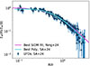 |
Fig. D.1. Observed stellar surface density distribution for the six UFDs analyzed in this work as worked out in Sánchez Almeida et al. (2024a, their Fig. 1). It is well reproduced by the line-of-sight projection of the SIDM profile used in Sect. 3. The magenta line corresponds to the best fit using one such profile. The figure also includes the polynomial fit to Σ★(R) given by Sánchez Almeida et al. (2024a, the solid cyan line). Here R stands for the projected radial distance from the center of the galaxy, and b is a radial scaling factor, different for the different dwarfs, that allows the whole set of dwarfs to collapse to a single shape. |
All Figures
|
Fig. 1. Time evolution of SIDM halos according to Yang et al. (2024). The timescale is parameterized in terms of the core-collapse timescale, tcc – Eqs. (3) and (7). The halos start off as NFW profiles of characteristic density and radius ρs0 and rs0, respectively. (a) Radial density at different timesteps going from almost the initial conditions (tage/tcc = 0) to core-collapse (tage/tcc = 1), including the formation of a maximum core (tage/tcc = tc/tcc ≃ 0.12). Profiles before the maximum core formation (tage ≤ tc) are represented as dashed lines whereas profiles after this core-formation are shown as solid lines. (b) Same profiles as (a) but normalized to the central density and to the core radius defined in Eq. (6). The black bullet symbol indicates the location of the core radius. (c) Time variation of the true core (the blue solid line; rc in Eq. (17)) and of the model core (the orange dashed line; r′c in Eq. (15)). (d) Time variation of the central density (the blue solid line; ρSIDM(0)) and of the characteristic density (the orange dashed line; ρs′ in Eq. (15)). The green arrow in (c) and (d) marks the timescale for maximum core formation. |
| In the text | |
|
Fig. 2. Monte Carlo simulation used to estimate the SIDM cross sections required to account for the DM cores of UFDs. The cross sections depend on a number of poorly constrained parameters (the parameters in Eq. (10)). The Monte Carlo simulations allow us to propagate their uncertainties on σH/m/βage (the gray histogram) and, via Eq. (9), on the cross section σ/m. The blue histogram represents the distribution assuming the UFDs are in the process of forming the core, whereas the green histogram assumes that DM is evolving into the core-collapse phase. The vertical dashed lines mark the 2.3% and 97.7% percentiles used to constrain the range of viable cross sections given in Eq. (11). See the main text for further details. |
| In the text | |
|
Fig. 3. SIDM cross sections found in the literature versus a representative relative velocity of the DM particles in the observed object. See Appendix A for the full references explaining that σ/m and “Velocity” have different meanings in the different works, which may explain part of the scatter. The value provided by the UFDs analyzed in this work is shown with the red circle with error bars. The two times symbols represent the median of the core formation and the core-collapse distributions shown in Fig. 2. The solid lines corresponds to the analytical form in Eq. (18), where σ0/m, w0, w1 = 30 cm2 g−1, 0, 80 km s−1 (the red line), 3 cm2 g−1, 0, 200 km s−1 (the blue line), and 11 cm2 g−1, 60 km s−1, 45 km s−1 (the black line). |
| In the text | |
|
Fig. 4. Stellar core radius versus stellar mass as predicted by the simple model presented in Sect. 3. Each line shows the variation in r★c with M★ when the DM halo mass goes from 107 to 1014 M⊙. The type of line depends on whether the corresponding profile is in the core-formation phase (tage < tc; dashed line) or the core-collapse phase (tage > tc; solid line). The parameters that define the cross sections are given in the inset, with the actual velocity dependence represented in Fig. 5 with the same color code employed here. Observations of r★c versus M★ are represented as symbols, each one corresponding to an individual object. The measurements are labeled in the inset, with the UFDs analyzed in this work appearing under the label SA+24. The link between labels and references is specified in Appendix C. The figure also includes the theoretical expectations from stellar feedback on CDM halos from Lazar et al. (2020, the gray band and solid line). |
| In the text | |
|
Fig. 5. Cross sections used to compute r★c(M★) in Fig. 4. The color code used here and in Fig. 4 is the same. The range of velocities highlighted with thicker lines corresponds to the range of effective velocities (Eq. (13)) when the halo masses go from 107 to 1014 M⊙, as used in Fig. 4. |
| In the text | |
|
Fig. 6. Central density of the SIDM profiles used in Fig. 4 versus the stellar core radius. The color code employed in Figs. 4 and 5 is also used here. As in Fig. 4, the line is dashed or solid depending on whether the corresponding profile is in the core-formation phase (dashed line) or the core-collapse phase (solid line). The figure also includes a number of observed densities for UFDs and dSph collected by Silverman et al. (2023, their Fig. 10). The range of central densities observed in UFDs is covered by the SIDM simulations, both in the core-formation and the core-collapse phase. The increase in the central density with decreasing radius is consistent with the observations that the product central density times the core radius tends to be constant regardless of the DM halo mass, with a value of around 44 M⊙ pc−2. This trend is represented as the dotted red line, assuming rc ≃ r★c. |
| In the text | |
|
Fig. 7. Effect of the uncertainty in various parameters defining the toy model presented in Sect. 3. We use two reference models, one with a high cross section (lemon orange) and one with a low cross section (cyan). They are represented in Figs. 4–6 with the same color. These reference models are drawn with solid lines, whereas the shaded regions show the uncertainties in the stellar mass-to-halo mass relation. The dotted lines employ a different concentration-to-halo mass relation than the toy model. See the main text for further details. |
| In the text | |
|
Fig. 8. Comparison between the thermalization radius (rte; Eq. (21)) and the stellar core radius (r★c). When the cross section is small (σ0/m = 0.3 cm2 g−1; the cyan lines), then rte and rc are similar, particularly in the region of interest for UFDs, where M★ < 106 M⊙. On the contrary, rte ≫ r★c for large cross sections (σ0/m = 400 cm2 g−1; the lemon yellow lines). For reference, the characteristic radius of the original NFW (rs; the dotted red line) and the virial radius (rvir; the dotted-dashed red line) are included. |
| In the text | |
|
Fig. B.1. Piecewise M★ = M★(Mh) used in Sects. 3 and 4 (the dashed lines; Eqs. [B.1] and [B.2]). A polynomial seamlessly joins the relationships worked out by Behroozi et al. (2013, high mass) and by Kim et al. (2024, low mass). For additional details, see Appendix B. |
| In the text | |
|
Fig. D.1. Observed stellar surface density distribution for the six UFDs analyzed in this work as worked out in Sánchez Almeida et al. (2024a, their Fig. 1). It is well reproduced by the line-of-sight projection of the SIDM profile used in Sect. 3. The magenta line corresponds to the best fit using one such profile. The figure also includes the polynomial fit to Σ★(R) given by Sánchez Almeida et al. (2024a, the solid cyan line). Here R stands for the projected radial distance from the center of the galaxy, and b is a radial scaling factor, different for the different dwarfs, that allows the whole set of dwarfs to collapse to a single shape. |
| In the text | |
Current usage metrics show cumulative count of Article Views (full-text article views including HTML views, PDF and ePub downloads, according to the available data) and Abstracts Views on Vision4Press platform.
Data correspond to usage on the plateform after 2015. The current usage metrics is available 48-96 hours after online publication and is updated daily on week days.
Initial download of the metrics may take a while.