| Issue |
A&A
Volume 705, January 2026
|
|
|---|---|---|
| Article Number | A51 | |
| Number of page(s) | 24 | |
| Section | Extragalactic astronomy | |
| DOI | https://doi.org/10.1051/0004-6361/202555306 | |
| Published online | 06 January 2026 | |
NGC 6860, Mrk 915, and MCG -01-24-012
II. Inflowing and outflowing cold molecular gas and the connection with ionized gas in Seyfert galaxies
1
Zentrum für Astronomie der Universität Heidelberg, Astronomisches Rechen-Institut, Mönchhofstr 12-14, D-69120 Heidelberg, Germany
2
Departamento de Astronomia, Universidade Federal do Rio Grande do Sul, IF, CP 15051, 91501-970 Porto Alegre, RS, Brazil
3
Astronomy Department, Universidad de Concepción, Barrio Universitario S/N, Concepción 4030000, Chile
4
Observatorio Astronómico Nacional (OAN-IGN) - Observatorio de Madrid, Alfonso XII, 3, 28014 Madrid, Spain
5
Departamento de Física, CCNE, Universidade Federal de Santa Maria, 97105-900 Santa Maria, RS, Brazil
6
Centro de Astrobiología (CAB), CSIC-INTA, Ctra. de Ajalvir km 4, Torrejón de Ardoz, 28850 Madrid, Spain
7
Finnish Centre for Astronomy with ESO, University of Turku, 20014 Turku, Finland
★ Corresponding author: This email address is being protected from spambots. You need JavaScript enabled to view it.
Received:
25
April
2025
Accepted:
5
November
2025
Abstract
We present a study of the cold molecular gas kinematics in the inner ∼4–7 kpc (projected sizes) of three nearby Seyfert galaxies with active galactic nucleus (AGN) luminosities of ∼1044 erg s−1 using observations of the CO(2–1) emission line obtained with the Atacama Large Millimeter/submillimeter Array (ALMA) at ∼0.5–0.8″ (∼150–400 pc) spatial resolutions. After modeling the CO profiles with multiple Gaussian components, we detected regions with double-peak profiles that exhibit kinematics distinct from the dominant rotational motion. In NGC 6860, a molecular outflow surrounding the bipolar emission of the [O III] ionized gas is observed extending up to Rout ∼ 560 pc from the nucleus. There is evidence of molecular inflows along the stellar bar, although an alternative scenario involving a decoupled rotation in a circumnuclear disk (CND) can also explain the observed kinematics. Mrk 915 shows double-peak CO profiles along one of its spiral arms. Due to the ambiguous orientation of its disk, part of the CO emission can be interpreted as a molecular gas inflow or an outflow reaching Rout ∼ 2.8 kpc. MCG -01-24-012 has double-peak profiles associated with a CND perpendicular to the [O III] bipolar emission. The CO in the CND is rotating while outflowing within Rout ∼ 3 kpc, with the disturbances possibly being caused by the passage of the ionized gas outflow. Overall, the mass inflow rates are larger than the accretion rate needed to produce the observed luminosities, suggesting that only a fraction of the inflowing gas ends up feeding the central black holes. Although we found signatures of AGN feedback on the cold molecular phase, the mass outflow rates of ∼0.09–3 M⊙ yr−1 indicate an overall weak impact at these AGN luminosities. Nonetheless, we may be witnessing the start of the depletion and ejection of the molecular gas reservoir that has accumulated over time.
Key words: ISM: jets and outflows / galaxies: active / galaxies: Seyfert / quasars: individual: NGC 6860 / quasars: individual: Mrk 915 / quasars: individual: MCG -01-24-012
© The Authors 2026
 Open Access article, published by EDP Sciences, under the terms of the Creative Commons Attribution License (https://creativecommons.org/licenses/by/4.0), which permits unrestricted use, distribution, and reproduction in any medium, provided the original work is properly cited.
This article is published in open access under the Subscribe to Open model. This email address is being protected from spambots. You need JavaScript enabled to view it. to support open access publication.
1. Introduction
Among the main physical processes that influence the evolution of galaxies are those occurring in active galactic nuclei (AGNs), which are ignited when matter is accreted into the supermassive black hole (SMBH) at the center of a host galaxy. Depending on the accretion rate, the energy can be released as radiation and winds from the accretion disk (radiative or quasar mode) or jets of highly energized particles (jet or mechanical mode) (Heckman & Best 2014). How effectively this energy couples with the host galaxy’s interstellar medium (ISM) is still a matter of debate. The net effect on the galaxy may lead to a suppression of the local star formation rate (SFR) in some objects (negative feedback, e.g., Wylezalek & Zakamska 2016; Cicone et al. 2014) or an increase in the SFR in others (positive feedback, e.g., Gallagher et al. 2019; Maiolino et al. 2017).
One way to gauge the effect of feedback on the galaxy is to measure the mass outflow rate and its power (Harrison et al. 2018) and understand which aspects influence the accretion processes (Storchi-Bergmann & Schnorr-Müller 2019). Historically, most studies have used ionized gas to search for these feedback effects (e.g., Spence et al. 2018; Dall’Agnol de Oliveira et al. 2021). However, the ionized phase constitutes only part of the gas in the ISM, which emphasizes the necessity of accounting for the impact on other gas phases (Cicone et al. 2018).
An important phase to be studied is the cold molecular gas phase, which experiences temperatures below ∼100 K and is the main ingredient for star formation (Veilleux et al. 2020). If the AGN feedback kinematically disturbs the gas in this phase, the affected molecular content might not meet the physical condition required to form new stars, which can be viewed as a direct impact on the ISM. To quantify that, one can search for signs of disturbances in the cold molecular gas using emission lines that trace the total cold H2 amount, such as the CO(2-1) molecular emission line (Bolatto et al. 2013b).
In the past two decades, evidence of AGN negative feedback in the cold molecular phase has emerged. In luminous sources with AGN bolometric luminosities of LAGN ≳ 1045 erg s−1, barely resolved observations have indicated large mass outflow rates of ∼ 102–103 M⊙ yr−1 (e.g., Feruglio et al. 2010; Cicone et al. 2014). However, in studies using higher spatial resolution data (scales of 10–100 parsecs), the measured effect appears to be lower, with values of ∼ 10–102 M⊙ yr−1 (e.g., Ramos Almeida et al. 2022; García-Burillo et al. 2014). For low- and medium-luminosity objects, LAGN ≲ 1045 erg s−1, a wide range of resolved outflow rates of Ṁmol,out ∼ 0.1–102 M⊙ yr−1 have been reported (e.g., García-Burillo et al. 2014; Oosterloo et al. 2017; Audibert et al. 2019; Alonso-Herrero et al. 2019; Slater et al. 2019; García-Bernete et al. 2021; Dall’Agnol de Oliveira et al. 2023; Alonso Herrero et al. 2023).
This work focuses on the low-luminosity regime by studying the CO(2-1) cold molecular gas kinematics of three nearby Seyfert galaxies: NGC 6860, Mrk 915, and MCG -01-24-012. The paper is organized as follows. Sections 2 and 3 describe the sample, the observations, and the archival data used. The methodology used for the analysis is explained in Sect. 4, with additional details in Appendices A–F. We analyze and discuss each object individually in the Sects. 6 (NGC 6860), 7 (Mrk 915), and 8 (MCG -01-24-012). The general discussion and conclusions are outlined in Sects. 9 and 10. Unless otherwise specified, all velocities are in the kinematic local standard of rest (LSRK). The luminosity distances and angular scales were calculated from the systemic redshift for a H0 = 70 km s−1, ΩM = 0.3 and ΩΛ = 0.7 cosmology.
2. Sample
The three Seyfert galaxies studied here, NGC 6860, Mrk 915 and MCG -01-24-012, have AGN bolometric luminosities in the range of LAGN ∼ 1043.6–1044.8 erg s−1, with redshifts of 0.014 ≲ z ≲ 0.025. These are galaxies with prominent stellar structures, such as spiral arms, rings, and bars. Their hosts have stellar masses in the range of M* ∼ 109.6–1010.3 M⊙, with black hole masses of MBH ∼ 107.1–108.4 M⊙ (see Table 1). A literature review and specific information about each object are provided below. The three galaxies are presented in color-composite images in Fig. 1, where we can observe their local environment.
General information about the sample.
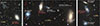 |
Fig. 1. Color-composite images from DESI Legacy Survey Sky Viewer showing the local environment of NGC 6860 (left), Mrk 915 (middle) and MCG -01-24-012 (right), with squares marking the FoV of Figs. 2a, 3a and 4a. The spectroscopic redshifts of the brighter sources correspond to the preferred values from the NASA/IPAC Extragalactic Database. North is up and east is left in this and the remaining figures in the paper. |
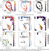 |
Fig. 2. Maps of NGC 6860. (a) Spatial distributions of the CO(2-1) moments maps of the observed spectral profile, with M0 corresponding to the integrated flux, M1 tracing the mean radial velocity, and M2 representing the velocity dispersion of the CO profile. (b) Maps of the parameters of the two Gaussian components fit the CO(2-1) profiles: c1 (top row) and c2 (bottom row). The columns correspond to distributions of the flux (left), the LoS velocity (middle), and the velocity dispersion (right). In the bottom row, contours outline the full CO(2-1) extent (in gray) and the double-peak region (in black). In the bottom-left map, we added dashed lines representing the spiral arms (orange), the stellar bar (yellow), and the ring (sky-blue), as identified in Paper I. The letters A – E in the lower-left panel show the locations of the spaxels used as examples of fits in Fig. 5. For this and all other maps in the paper: North is up and east is left. The coordinates are relative to ALMA millimeter continuum peak (black cross marks, see Table 1), assumed to be to the galactic nucleus. The gray ellipses correspond to the ALMA beam size of the observation. The inclined black dotted line is the major axis of the global kinematic model. |
The relation between the CO(2-1) cold molecular versus [O III]λλ4959,5007 ionized gas flux distributions of these objects were presented in Dall’Agnol de Oliveira et al. (2025, hereafter Paper I). The analysis revealed a spatial anticorrelation between the two gas phases, suggesting local CO depletion caused by AGN feedback.
2.1. NGC 6860
NGC 6860 is a barred spiral (R’)SB(r)b galaxy with both an inner and an outer stellar ring (de Vaucouleurs et al. 1991). The nuclear spectrum was classified as Seyfert 1.5 by Lipari et al. (1993). Nonetheless, Winter & Mushotzky (2010) raised the possibility of it being a changing-look AGN (Matt et al. 2003), given the variability in X-ray flux and shape relative to previous observations (Winter et al. 2008). Variations in the shape of the UV continuum and the H α broad line region (BLR) profile were also observed in the past (Lipari et al. 1993).
There is no bright companion near NGC 6860 (left of Fig. 1). The larger object at small angular distances is the unknown diffuse galaxy LEDA 166191, separated by ∼3.5′. The nearest object with a similar redshift is 2MFGC 15362 (z = 0.01495), located at ∼15′ to the southeast of NGC 6860.
Lipari et al. (1993) presented a detailed analysis for this luminous IR source, using long-slit observations and narrow-band images centered on [O III]λλ4959,5007 (hereafter, just [O III]) and H α+[N II]λλ6548,6583. In the inner stellar ring, the [O III]/(H α+[N II]) excitation map shows values in agreement with stellar-like ionization. Inside the ring, the above line ratio is AGN-like, with the nuclear spectrum showing a broad Hα component, denoting the presence of a BLR. The optical continuum shows old stellar population features in the spectra from regions along the bar, between the ring and the nucleus. In the ring, the spectra are more typical of H II regions.
2.2. Mrk 915
Mrk 915 is a spiral Sa galaxy (Malkan et al. 1998) possessing a variable Seyfert nucleus. It has been classified as type 1.5–1.9, depending on the presence of H α and/or H β BLR components (Goodrich 1995; Bennert et al. 2006; Trippe et al. 2010).
Mrk 915 is part of a triple system, along with other two bright sources (Karachentseva & Karachentsev 2000): MCG -02-57-024 and MCG -02-57-022, separated by angular distances of ∼2′ and 4.3′, respectively (middle of Fig. 1). Moreover, there is another source (LEDA 951231) ∼1′ to the west of Mrk 915. It has long tidal features appearing to extend up to MCG -02-57-022 at southwest. We only found a highly uncertain photometric redshift for this object: zphot = 0.041 ± 0.02 (Zhou et al. 2023, DESI-DR9). Hence, we cannot confirm if this object is part of the system.
Muñoz Marín et al. (2009) presented HST imaging observations in the Near Ultraviolet (NUV) for Mrk 915. The extended NUV flux distribution is probably due to the [Ne IV]λλ3346,3426 emission lines since it is equivalent to the scaled [O III] distribution, although an NUV excess is observed at the nucleus (Muñoz Marín et al. 2009). Therefore, in addition to nuclear activity, a nuclear starburst could also contribute to the NUV excess. However, in this region, the gas line ratios indicate an AGN-like excitation (Bennert et al. 2006), with the optical continuum being consistent with an elliptical galaxy template, indicating a dominant old stellar population (Trippe et al. 2010).
Mrk 915 has multiple X-ray observations (Trippe et al. 2010; Severgnini et al. 2015; Serafinelli et al. 2020). Ballo et al. (2017) identified X-ray variability in intensity, but not in the shape of the continuum. Their models advocates for the presence of warm absorbers, but with the continuum variability being mostly caused by an intrinsic variation in nuclear power.
2.3. MCG -01-24-012
MCG -01-24-012 is a spiral SAB(rs)c galaxy showing both an inner stellar ring and weak bar (de Vaucouleurs et al. 1991). Its nucleus was originally classified as a type 2 AGN (e.g., Véron-Cetty & Véron 2006), but a broad FWHM ∼ 2000 km s−1 component was later detected in the Pa β emission line (e.g., Onori et al. 2017), as well as a weak broad component in the H α line (La Franca et al. 2015). The “hidden” BLR component in the Balmer lines may be a consequence of the optical spectral region being more attenuated relative to the infrared by the material in the host galaxy (e.g., Ricci et al. 2022).
MCG -01-24-012 has two close and bright companion galaxies: MCG -01-24-011 and MCG -01-24-013, separated by angular distances of ∼1.3′ and 2.7′, respectively (see (Fig. 1)). Together, they appear to form a triple system, probably gravitationally bound due to the small differences in redshift.
The X-ray continuum of MCG -01-24-012 has been studied in the past (Malizia et al. 2002; Winter et al. 2009), showing moderate variability (Middei et al. 2021). Besides the Fe Kα 6.4 keV fluorescent emission line, there is an absorption feature detected at ∼7.5 KeV (Malizia et al. 2002). If corresponding to the Fe XXVI Lyα line (rest 6.97 keV), this feature could originate from a powerful nuclear outflow with velocity Vout ∼ 0.06 c (Middei et al. 2021).
3. Observations
We observed our sources using the Atacama Large Millimeter/submillimeter Array (ALMA) during Cycle 6 (ID: 2018.1.00211.S), with one of the spectral windows (SPW) centered on the CO(2-1) emission line (230.538 Hz rest frequency). The final continuum-subtracted cubes have channel widths of Δv ∼ 10.2 km s−1, with a σrms noise at their field-of-view (FoV) centers ranging between ∼0.4 and 0.7 mJy beam−1. The FWHM of the synthesized beams of NGC 6860, Mrk 915, and MCG-01-24-012 are, respectively, 0.41″ × 0.56″ (∼150 pc), 0.78″ × 0.88″ (∼400 pc) and 0.47″ × 0.6″ (∼200 pc). The size of the individual spaxels are 0.076, 0.16, and 0.087″, in the same order.
We also used archival data from the Hubble Space Telescope (HST) and Very Large Array (VLA). The HST FR533N narrow-band images (Schmitt et al. 2003, ID: 8598,), centered on the [O III]λλ4959,5007 emission lines (hereafter [O III]), were used to trace the ionized gas flux distribution. The VLA 8.46 GHz (3.54 cm) radio images (Schmitt et al. 2001, proposal ID: AA226), was used to look for signatures of radio jets. We also collected archival DECam (Dark Energy Camera) g- and z-bands images from the Data Release 10 of the DESI (Dark Energy Spectroscopic Instrument) Legacy Imaging Surveys. Details about observations and reductions of the ALMA and the archival data are given in Paper I.
4. Analysis
4.1. Moments from CO(2-1)
An overview of the spatial distribution and kinematics of the molecular gas can be obtained from the moments of the CO line profiles (as described in Appendix B). Figures 2a, 3a and 4a show the resulting maps of the moments in the first row: for NGC 6860, Mrk 915, and MCG -01-24-012, respectively. The 0-th moment (M0) is the distribution of the line flux, the first moment (M1) is the intensity-weighted mean of the line of sight (LoS) velocity, and the second moment (M2) is the square root of the intensity-weighted mean of the squared velocity dispersion (e.g., Ramakrishnan et al. 2019). M1 traces the projected centroid velocity of the CO clouds inside a given region, while M2 traces the width of the profiles (sensitive to kinematic disturbances). For a line profile perfectly modeled by a single Gaussian, M1 and M2 are the centroid velocity and the velocity dispersion of the gas, respectively.
4.2. Dust attenuation and orientation of the disk
The interpretation of the kinematics will depend on knowing which are the near and far sides of the galaxies’ disks: the orientation relative to the plane of the sky. For this, we assumed that the side where the optical stellar continuum is more attenuated by dust is the near side. This is based on the overall assumption that, close to the photometric minor axis (measured in optical broadband images), the presence of dust lanes is more “noticeable” on the near side of the disk due to the contrast with the background stellar light from the bulge (Iye et al. 2019). We also checked if the resulting orientation agrees with the galaxy having trailing spiral arms. If the molecular gas and stars co-rotate, the CO(2-1) first moment maps (M1) can be used to gauge the sense of rotation of the spiral arms (middle column of Figs. 2a, 3a and 4a). For reference, the photometric major axes of NGC 6860, Mrk 915, and MCG -01-24-012 are 34, 162, and 38° (mean position angles), respectively (Schmitt & Kinney 2000, from broadband B images).
We used the ratio between the DECam g- and z-band images as a proxy for dust attenuation in the host galaxy, since the extinction is stronger at bluer wavelengths (e.g., Mezcua et al. 2015). The results are shown in Fig. C.1. Inspecting these maps, we identified that the near sides of MCG -01-24-012 and NGC 6860 are to the southeast and northwest, respectively. These orientations agree with the galaxies having trailing arms. For Mrk 915, the orientation is ambiguous: while the dust attenuation map indicates that the near side may be to the southeast, a trailing arms scenario implies that the near side of the disk is to the northwest. We discuss this scenario in Appendix C. Both orientations for the Mrk 915’s disk were considered in the analysis done in Sect. 7.
4.3. CO(2-1) emission-line fitting
In all sources, CO(2-1) emission-line profiles show double peaks near the nucleus, typically within a radius of ∼1 kpc, but also in a few locations far from the nucleus. We tentatively attribute the origin of these two peaks as coming from different molecular gas clouds with distinct global kinematics. We modeled the CO profiles with multiple Gaussian components using the PYTHON package IFSCUBE (Ruschel-Dutra et al. 2021). For each spaxel (sizes of 0.08–0.16″ ∼ 20–80 pc), the program returns the Gaussian parameters from the model that minimizes the residuals. The optimization is done by using the Sequential Least Squares Programming (SLSQP) method from SCIPY.MINIMIZE.
To account for the presence of double peaks, each spectrum was fit with two models: a single Gaussian (1g), and two Gaussian curves (2g). Each Gaussian component is characterized by its amplitude (Sν,CO), LoS velocity (vCO), and velocity dispersion (σCO). The velocity-integrated flux (SνΔvCO) in units of Jy km s−1 can be converted to luminosities in units of K km s−1 pc−2 (L′CO) and L⊙ (LCO) by following Solomon et al. (1997, Eqs. 1 and 3).
Gaussian components with a signal-to-noise ratio (S/N) below 3 were discarded. Therefore, 2g models were selected over 1g ones when both Gaussian components (of the 2g model) exceeded the above S/N criterion. Since neighbors’ spaxels are non-independent inside the beam area, isolated spaxels with 2g were also discarded. Examples of CO profile fits are shown in Fig. 5. Maps of the best-fit parameters are displayed in Figs. 2b, 3b and 4b, showing the distributions of the flux, LoS radial velocity, and velocity dispersion of each component. We also generated a grid of spectra in Fig. A.1 (Appendix A), which allows for a comparison of CO profiles inside and outside the identified double-peak regions.
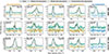 |
Fig. 5. Example of the model multiple Gaussian models fit to the CO(2-1) profiles of individual spaxels (0.076–0.16″ sizes), one row per object. The first four columns (A to D) show examples where two Gaussian components were preferred over a single component, as in the last column (E). The spatial positions (relative to the nucleus) of each spaxel are shown at the top of each panel and are marked in Figs. 2a, 3a and 4a (blue letters in the lower left panels). The lines represent: original data (bluish-green); one Gaussian component models (in blue); two Gaussian models (in orange), along with their individual components (in black dashed). The residuals of both models are shifted downward in the plots. The y-axes are in units of S/N. The horizontal dotted line corresponds to S/N = 3 and is highlighted since this was the threshold used to discard components. |
4.4. Position-velocity diagrams
Figure 6 shows the CO(2-1) position-velocity (PV) diagrams for three orientations: (1) Along the kinematic major axes (see Section 4.5): Position angles (PAs) of 40, −7, and 32°, for NGC 6860, Mrk 915, and MCG -01-24-012, respectively. (2) Along the minor axes, perpendicular to the above orientations. (3) Along a third direction, covering most of the double-peak region: PAs of 16, −36, and 0°, for NGC 6860, Mrk 915, and MCG -01-24-01.
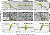 |
Fig. 6. Position-velocity maps for the CO(2-1) of each object for 1″-width pseudo-slits along three different positions: kinematics major and minor axis (first two columns) and along the double-peak (dp) region (last column). We added the individual LoS velocities obtained for the Gaussian components c1 (blue circles) and c2 (orange circles) fit to the spectral profiles. The bluish-green lines correspond to the global rotating disk model fit to the single-peak (sp) region (first three rows in Table 2). For NGC 6860, three models are shown, which were fit using data from the ring (bluish-green line), from the bar (dot-dashed black line), and combining data from both ring and bar (long dashed black line). For MCG -01-24-012, we also added curves from two models fit in the double-peak region, one letting the PA free (short dashed black line) and the other with PA = 0° (dotted black line). |
4.5. Kinematic modeling
In all sources, most of the CO profiles far from the nucleus show narrow single-component profiles. These regions in the M1 moment maps (Figs. 2a, 3a and 4a) display a typical disk rotation pattern and low M2 values (≲15 km s−1), indicating that they might be tracing gas rotating in the galaxy disk.
To verify this, we fit a 2D disk rotation model (Bertola et al. 1991) to the data. More specifically, we fit the LoS velocity distribution map in regions showing only single components dominated by rotation: the LoS velocity map of the c1 component (vc1), excluding the region with double-peak profiles (see detailed description in Appendix D).
The best-fit parameters of the models are displayed in the first three rows of Table 2. Maps of the data, best-fit model, and residuals are shown in Fig. 7 (first three columns), with a zoom-in of the residuals from both components displayed in the last two columns. They are also represented by bluish-green solid lines in the PV diagrams of Fig. 6.
Parameters of the 2D disk models.
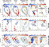 |
Fig. 7. Comparison between the CO(2-1) data obtained from the Gaussian decomposition of the profiles and the rotating 2D disk model (first three rows in Table 2). The first three columns show the distributions of the LoS velocity of the c1-component (vc1), the best-fit rotation model, and the residuals from the fit. The model was fit to the single-peak region of the vc1 data (masked regions not shown). An additional mask was used for the inner regions of NGC 6860, restricting the fit to regions dominated by rotation in the disk. The last two columns are a zoom-in showing residuals of each component (c1 and c2), with the models extended to the double-peak region. The black contours encircle the masked regions with double-peak CO profiles, while the gray contours show the full data extent. The dashed lines identify stellar structures: bars (yellow), spirals (orange), and rings (sky-blue). |
For NGC 6860, the CO data in the bar were also masked during the fit, with only data in the ring being used for the global rotating disk modeling. This was done because the kinematics in the bar and the ring diverge noticeably, with a simple rotating model being unable to account for both dynamics. We note that including the data from the bar in a global fit would not significantly change the results (see the fourth row in Table 2). The last three rows of the table refer to alternative models discussed in Sects. 6.2.2 and 8.2.
4.5.1. Identification of the components in the double-peak region
In the region with double-peak profiles, the origin of the emission of each component (leading to the double peaks) is not known a priori. As a first identification criterion, we assumed that one of them is tracing gas dominated by rotation. Therefore, we named the component with lower absolute residuals relative to the disk model “c1.” We call the other component “c2,” and in principle, it traces the emission from disturbed gas (e.g., from outflows or inflows). Whenever needed, we added a second criterion for selecting c1: we visually selected it to be the one that minimizes the discontinuity in the c1 maps. In some cases, none of the components follow the global disk rotation pattern (e.g., CO along the bar in NGC 6860, as discussed in Sects. 6.2.1 and 6.3). We therefore emphasize that the c1 component does not solely trace gas rotating in the galaxy disk.
4.6. Schematic models
Figure 8 displays schematic models for the three objects. They help visualize the scenarios discussed in Sects. 6–8. We refer to the upper left panels of Figs. 2a, 3a and 4a for more detailed contours comparing the flux distribution of [O III] and CO(2-1).
 |
Fig. 8. Schematic models for our proposed scenarios of NGC 6860, Mrk 915, and MCG -01-24-012. The second row corresponds to a zoom-in in the central regions. Due to the ambiguous orientation of the Mrk 915 disk (see Appendix C), we added both scenarios of spiral arms motion: trailing and leading. The contours represent the flux distribution of: cold molecular gas from CO(2-1) M0 (bluish-green), ionized gas from HST [O III] (reddish-purple), VLA 3.6 cm radio (blue), and the CO double-peak region (black). For a better view, we plotted only a few contour levels and manually cleaned isolated ones. Stellar structures are drawn in dashed lines: spiral arms (in orange), stellar rings (sky-blue), and bars (yellow). The gray “3D” planes correspond to the plane of the global rotating disk model. We also added “3D” bipolar ionized cones to represent possible orientations of these structures. The senses of rotation of the spirals are shown in orange dashed arrows, assuming that they “follow” rotation of the CO. The solid arrows represent the direction of motion of: components c1 (blueish-green) and c2 (black) of the CO(2-1), ionized gas (reddish-purple) and radio-jets (blue), with curved lines representing rotation. We added question marks to represent that we can only confirm the kinematics of the [O III] using resolved integral-field observations, and the same for the possible radio jets that need deeper and higher spatial resolution observations. In the double-peak regions, we added one arrow for each component. In particular, for MCG -01-24-012, we tried to represent that both components are dominated by rotation, with each one having an extra positive/negative radial velocity “kick” due to the CO being disturbed equatorially by the ionized outflow. |
5. Results: Global rotation
The bulk of the cold molecular gas is rotating in a disk, particularly in the outer regions where the profiles are narrower. The mean values of residuals in the single-peak CO region are ∼ 20–30 km s−1, and about ∼10% of the maximum LoS velocities in the regions with highest velocities in the disk model (see third column in Fig. 7). For comparison, using formulas from Lenz & Ayres (1992), we estimated a mean uncertainty in the fit LoS velocities (Gaussian centers) of ∼ 2–3 km s−1, with maximum uncertainties of ∼ 10 km s−1 in regions with low S/N. We believe the latter value better reflects the uncertainties, as it matches the channel widths of the cube. Therefore, the maximum residuals are a factor of about two to three above the uncertainties. This might be a sign that, although our model for the global rotation reproduces well the kinematics in the single-peak regions, local forces also influence the molecular gas. Possible candidates might be local gravitational forces associated with stellar structures, since the CO is mostly observed close to stellar rings, bars, and spirals. Although not shown here, dust lanes might also play a role (König et al. 2014).
However, some regions present prominent distinct kinematics, reaching residual LoS velocity values of up to ∼100 km s−1, as shown by the PV diagrams in Fig. 6. Along the kinematic minor axes, we observe non-zero velocity emission in all sources, which has been used as a signature of non-circular motions (e.g., Ramos Almeida et al. 2022). These regions were better modeled using two Gaussian components (see the individual LoS velocity values (circles), reinforcing that the double-peak region is tracing disturbed CO kinematics. In the following Sections 6–8, we analyze the three sources in our sample individually.
6. Results: NGC 6860
6.1. NGC 6860: CO in the stellar ring
The CO emission in NGC 6860 is observed along its inner stellar ring and bar. In particular, the CO gas kinematics in the ring is dominated by rotation (see Fig. 7).
In addition, at ∼7.6″ to the north of the NGC 6860’s nucleus (in the ring, at the intersection with the bar), there is a region with double-peak CO(2-1) profiles. Both c1 and c2 components present low LoS velocity residuals relative to the disk model: less than ∼20 km s−1 in absolute values (last two columns of Fig. 7). Their residuals seem to follow the pattern of the gas in neighboring spaxels, with its kinematics probably being dominated by rotation. For the CO gas traced by these components, we assumed that: c1 is only rotating, since it its lower relative residuals; c2 is rotating, but suffers a small local gravitational disturbance, probably introduced by the nearby spiral and/or the bar. From now on, we concentrate our analysis on regions closer to the nucleus.
6.2. NGC 6860: CO in the stellar bar
A stellar bar structure, with a position angle PA ∼ 12°, lies within the ring (yellow dashed line in Fig. 2b). Along the inner part of this structure, we can observe CO emission (e.g., top-left panel of Fig. 2b). Below, we discuss two possible scenarios for the kinematics of molecular gas observed along this region.
6.2.1. NGC 6860: Possible inflowing CO clouds in the stellar bar
Along the NGC 6860 bar and inside a 4″ radius (∼ 1 kpc), the CO LoS velocity distribution of the component c1 shows high deviations relative to circular orbits (see Fig. 7), with maximum residuals of ∼ 75 km s−1. Given the negative values on the far side, and mostly positive on the near side, these residuals suggest inflows along the bar.
The presence of molecular inflows along the bar in the inner kiloparsec was already proposed by Lipari et al. (1993). Their hypothesis was based on the possible presence of an ionized gas inflow, concluded after analyzing the velocity residuals of [O III] and H α relative to a rotation disk model fit to the data. However, they assumed the northwest as the near side of the galaxy, but here we could better constrain it to be in the southeast (see Sect. 4.2). Using our disk orientation, these ionized gas residuals should be interpreted as ionized gas outflow.
For a better understanding of the dynamics of NGC 6880, we generated an additional PV diagram in Fig. 9, reproducing the slit configuration of Lipari et al. (1993). We added the LoS values1 from the stellar Ca II K and Na I D absorption lines and ionized gas emission lines [O III] and H α, together with our CO data and its kinematic models. Overall, the stellar and the ionized gas seem to follow the rotation model of CO in the ring. However, in the lower left quadrant, under 5″ of the nucleus (reddish-purple dotted line), the ionized gas shows velocity residuals. These are the residual originally detected by Lipari et al. (1993), which we reinterpret as coming from an ionized outflow (as discussed in the previous paragraph).
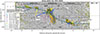 |
Fig. 9. Position-velocity map of NGC 6860, similar to Fig. 6, but for a position angle along the bar and with a slit width of 1.5″, matching the observations from Lipari et al. (1993). We added their observed LoS velocities from the stellar absorption lines of Ca II K (triangles) and Na I D (crosses) in reddish-purple color and the ionized gas emission lines of [O III] (star symbols) and H α (‘x’ markers) in sky blue. |
Assuming a constant gas inflow rate along the bar and an inclination of i = 57.7° (coplanar with the galaxy disk), we obtained a cold molecular mass inflow rates of Ṁmol,in ∼ 0.8–6 M⊙ yr−1 (see Table 3). For an inclination of i = 70°, the Ṁmol,in value would decrease by a factor of ∼ 1.7, while for i = 40°, it would increase by a factor of ∼1.9. The total inflowing molecular gas mass involved in the process is Mmol, in ∼ (1–9) × 107 M⊙, corresponding to volumetric number density of molecular clouds of nmol ∼ 3–30 cm−3. See Appendix E.1, for details on the calculation.
Inflow properties.
This range of nmol values is compatible with the results obtained for diffuse clouds by Luo et al. (2023). The presence of a more diffuse gas in the bar could be a consequence of the bar-induced turbulence and even help to suppress star formation inside the ring (e.g., Khoperskov et al. 2018; Scaloni et al. 2024). And indeed, the [O III]/(H α+[N II]) excitation map from Lipari et al. (1993) indicates AGN-like ionization in this region, without signs of star formation. Another proposed explanation is that the bar creates an inflow of gas, caused by a strong torque that drives the gas directly to the galactic center, where in some cases star formation is enhanced (e.g., Spinoso et al. 2017). However, we note that there is no evidence of nuclear star formation in NGC 6860 (Lipari et al. 1993).
Higher turbulence in the CO can also be induced by shear in the inflowing gas along dust lanes, as observed in the minor merger systems NGC 4194 (König et al. 2013) and NGC 1614 (König et al. 2014). Similarly to NGC 6860, ongoing star formation is not observed in these turbulent regions. However, part of the inflowing material in these two systems – probably associated with the recent galaxy interaction – ends up fueling ongoing star formation in other regions nearby, which does not seem to be the case for NGC 6860. Besides that, as shown in Fig. 1 and pointed out in Sect. 2.1, there is no clear sign of a recent merger in NGC 6860, although deeper broadband imaging observations may reveal a different picture. We cannot discard that part of the inflowing material will not be used to form new stars in the future, or that there is deeply embedded star formation happening in the central region. In Sect. 9.1, we show that only a fraction of the inflowing gas ends up feeding the AGN, and discuss whether we should expect to observe a reservoir of CO accumulating in the nucleus.
6.2.2. NGC 6860: Possible alternative scenario for the CO in the bar of a decoupled disk rotation
There is an alternative scenario to explain the CO kinematics along the bar, within ∼1 kpc from the nucleus: a decoupled rotation from the gas in the ring. This hypothesis was raised because the steep LoS velocities in the PV diagrams (Figs. 6 and 9) seem to be characteristic of a rotation (instead of inflows). Different scenarios have been proposed to explain a decoupled kinematics between the gas in the inner and outer regions, including infalling of new gas material from cosmological filaments and mergers with gas-rich dwarfs (e.g., Thakar & Ryden 1996). In these cases, the decoupled kinematics arise from a misalignment between the disk angular momentum of the gas in the galaxy disk and the arriving material.
To test this, we modeled the gas kinematics in this region with an independent rotating disk model (Bertola et al. 1991), fixing the systemic velocity but leaving the remaining parameters free. And, indeed, a rotating gas model can fit reasonably well the LoS velocities in the bar, as shown by the corresponding parameters maps in Fig. F.1 (in Appendix F) and the dashed-dotted black lines in the PV diagrams (Figs. 6 and 9). The best-fit parameters (see in Table 2) show a similar position angle to that of the ring (PA ∼ 40°), but with the plane of rotation having a higher inclination (i ∼ 69°).
The elongated CO emission distribution in the bar supports an internal inclined disk, although one might argue that this scenario would also require that the major axis be more aligned with the bar (PA ∼ 12°). Another argument against this alternative scenario is that the velocities of the stars and the ionized gas – in the bar – agree with the rotation model of CO in the ring (see Fig. 9). However, stars, ionized, and cold molecular gas do not necessarily need to have the same rotation pattern. The ionized and molecular gas can differ, for example, in the amplitude of the rotation velocity and the dispersion of the velocity (e.g., Levy et al. 2018). In the more pronounced cases, counter-rotation between gas and star is present (e.g., García-Burillo et al. 2000, 2003).
Since we cannot fully discard any of the above scenarios, we considered both explanations for gas in the bar traced by the component c1: inflows or decoupled rotation. Finally, we note that the latter hypothesis could be interpreted as a circumnuclear disk (CND), similar to the one in MCG -01-24-012 (see Sect. 8.2).
6.3. NGC 6860: A molecular outflow encasing the ionized one
There is another CO double-peak region, close to the nucleus and within a ∼1″ radius (see Fig. 2b). This region is located at the intersection between the [O III] bipolar cone and the CO gas distribution. The kinematics of the c1 component in this region is similar to the gas in the single-peak region around it, indicating that it is tracing inflowing gas or the CND motion, depending on the interpretation for the CO in the bar (see Sects. 6.2.1 and 6.2.2). Independent of the interpretation for c1, the emission from the c2 component is likely tracing outflowing molecular clouds: it shows negative residuals relative to the global disk rotation model, which are located at the near side of the disk (see Fig. 7, last column).
These outflowing molecular clouds are located at the border of the [O III] bipolar emission. This elongated ionized gas emission also has evidence of outflows from optical long-slit observations along the east-west direction (Bennert et al. 2006, PA = 85°): the ionized gas has negative LoS velocities at the near side and positive at the far side of the disk. In addition, the line ratios in the nuclear region are AGN-like (Bennert et al. 2006; Lipari et al. 1993). Therefore, in the nuclear region, the ionized gas outflow seems to be partly surrounded by a molecular one, traced by the c2 component in our CO(2-1) data, as represented in the first column of Fig. 8.
This suggests that in NGC 6860 the outflowing molecular clouds can only survive at the borders of the ionized cones, being destroyed closer to the ionization axis. This scenario is similar to what we observed in the Seyfert galaxy NGC 3281 (Dall’Agnol de Oliveira et al. 2023). Other objects presenting outflowing molecular clouds with a similar hour-glass morphology – although sometimes surrounding X-ray cavities or radio lobes – include the Milky Way (e.g., Veena et al. 2023), starburst galaxies (e.g., Bolatto et al. 2013a), radio jets/bubbles (e.g., Morganti et al. 2023; Zanchettin et al. 2023), galaxy clusters (e.g., Russell et al. 2017), and even newborn stars (e.g., Delabrosse et al. 2024; Nagar et al. 1997; Zhang et al. 2019). The existence of such scenarios in quite different astronomical environments suggests that these “onion-like” outflows might be common.
The above hypothesis relies on the assumption that outflows observed in both phases were launched at the same time. Another possible scenario would be that the CO clumps were ejected before, with the ionized gas being launched later and filling the gap left behind by the other phase. In this scenario, one might expect that the cold molecular outflow extent (∼ 1″) should be larger than the ionized one (∼1.3 ″), which does not seem to be the case. However, this is based on the assumption that both phases have the same outflow velocities and inclinations, which is not necessarily true. The opposite case, where the ionized gas had been ejected earlier, can also be considered. Besides that, we cannot discard that we might be missing part of the total molecular outflow content, which might be present in denser (e.g., as traced by HCN molecular lines), hotter phases (e.g., H2 near-infrared lines), and/or other CO isotopes (e.g., 13CO lines). Therefore, even though we favor a scenario where both the ionized and the cold molecular gas are being ejected together, with the latter only surviving at the border of the ionized cone, we cannot fully discard that other scenarios might better explain the observations.
Following Appendix E.2, the total molecular mass of the outflowing clouds in NGC 6860 is Mmol, out ∼ 0.6–5 × 10⁶ M⊙ (see Table 4). This corresponds to ∼0.7% of the total molecular mass in the galaxy observed within a radius of ∼13″. Assuming that outflow is coplanar to the galaxy disk (i = 57.7°), the de-projected maximum velocity and outflow extent are Vout ∼ 140 km s−1 and Rout ∼ 560 pc, respectively, with the molecular mass outflow rate being Ṁmol,out ∼ 0.1–1 M⊙ yr−1. For a different inclination of i = 70° (i = 40°), the Ṁmol,out value would decrease (increase) by a factor of ∼1.7 (∼1.9).
Outflow properties.
7. Results: Mrk 915
7.1. Mrk 915: CO along the spiral arms
The CO emission in Mrk 915 is distributed along its two inner spiral arms, extending up to a ∼15″ radius. Along the northwest spiral arm, we detected double-peak CO profiles in Mrk 915 in three regions spread approximately along a projected line (at PA ∼ −36°), starting at the nucleus and extending up to ∼5″ to the northwest (see Fig. 3b). Both c1 and c2 components in the two inner CO clumps show negative LoS velocities relative to the disk rotation model (middle column in Fig. 3b). Since the absolute LoS velocity residuals values of the c1 component are lower than those of c2 (Fig. 7), we assumed that the c1 component in the double-peak region is tracing gas rotating in the disk.
7.2. Mrk 915: CO in the double-peak region
The interpretation of the kinematics of the component c2 depends on the orientation of the disk, which we already noted is ambiguous (see Appendix C). Schematic models considering the two possible orientations are shown in Fig. 8, including the resulting spiral arms motion: trailing (second column) and leading (third). Independent of the orientation, the LoS velocity residuals are complex, showing negative values closer to the nucleus (covering the two nearest CO clumps under a ∼2.3″ radius) and positive at the farthest clump (at ∼5″ radius).
We chose to ignore the farthest CO cloud in our analysis. The decision was a consequence of the lack of a clear scenario that could properly explain the kinematics of the three c2-clumps in the double-peak region. This could be a consequence of the low S/N spectra of Mrk 915. Deeper observations might allow better modeling of disk rotation, yielding different LoS velocity residual values.
7.2.1. Mrk 915: Possible molecular inflow (leading arms scenario)
We can assume that the near side of the Mrk 915 disk is to the east (from the dust attenuation method, leading to a leading spiral arms scenario). In this case, the origin of the negative residuals of vc2 (from the two inner CO clumps) could be interpreted as coming from inflowing molecular clouds.
Following Appendix E.1, we obtained a molecular mass inflow rate along the one of the spirals of Ṁmol,in ∼ 0.09–0.8 M⊙ yr−1, involving a total molecular mass of Mmol, in ∼ (0.9–8) × 106 M⊙. This corresponds to volumetric number density of nmol ∼ 0.4–3 cm−3, which is an order of magnitude lower than the value obtained for NGC 6860. We assumed an inflow inclination of i = 66.5° (coplanar with the disk), for these calculations. For an inclination of i = 80° (i = 50°), the Ṁmol,in value would decrease (increase) by a factor of ∼2.5 (∼1.9). The same dependence on the inclination applies for mass outflow rate value (see this scenario in Sect. 7.2.2).
Given that Mrk 915 is part of a triple system (see Sect. 2.2 and Fig. 1), the gravitational influence of the two bright companions might have disturbed the gas in the host galaxy disk. If this gravitational influence leads to a significant loss of angular momentum in the gas, we may be currently observing the resulting CO inflow motion. We also note that, since both components are observed along the same LoS in the double-peak region, the “non-rotating” c2 might be tracing out-of-plane gas, which could be a consequence of material flowing from tidal streams of gas from these nearby companions.
7.2.2. Mrk 915: Possible molecular outflow (trailing arms scenario)
On the other hand, if the near side of Mrk 915 is to the west (agreeing with trailing arms), the origin of the c2 emission could be outflowing clouds. The large negative values of vc2 seem to favor this scenario, with mean projected residuals values of ∼ − 220 km s−1 in the nucleus. There is also a small elongation in the 3.6 cm radio, although along another direction (PA ∼ 220°), that could be associated with a radio jet (see Fig. 8). However, contrary to our other two sources, the [O III] emission is not bipolar, which would help identify a possible ionization axis.
Following this scenario (see Appendix E.2, for details), the total cold molecular mass of the outflowing clouds is Mmol, out ∼ 0.8–7 × 10⁶ M⊙, corresponding to 4% of the total mass of the gas in this phase. If we assume an outflow coplanar to the disk (i = 66.5°), we obtain a molecular mass outflow rate of Ṁmol,out ∼ 0.09–0.7 M⊙ yr−1, for an deprojected outflow velocity of Vout ∼ 300 km s−1 and radius of Rout ∼ 2.8 kpc. If we vary the inclination by ∼15°, the Ṁmol,out value would change by a factor of ∼2, analogous to the effect on Ṁmol,in (shown in Sect. 7.2.1).
In the schematic models shown in Fig. 8, we added two [O III] cones aligned with the [O III] emission. They were drawn assuming that the asymmetric [O III] elongation and the 3.6 cm emission radio are possibly tracing two distinct ionization axes, and considering that they could have partly destroyed the molecular gas. Maybe one of the [O III] elongations could be a relic of a previous AGN orientation, possibly associated with a galaxy interaction. In this case, the [O III] flux distribution would be a consequence of two distinct accretion events. Supporting this, we found signs of a possible tidal trail between Mrk 915 and one of its two nearby galaxy companions, as noted in Sect. 2.2 (see Fig. 1). Nonetheless, we emphasize that this is just a speculative scenario, and we do not have strong evidence in favor of it. Resolved integral field observations of the ionized gas should help to clarify the geometry and kinematics of the [O III] emitting gas.
8. Results: MCG -01-24-012
8.1. MCG -01-24-012: CO in the stellar ring and bar
The observed cold molecular gas – as traced by CO(2-1) – is observed along the ring and inside its radius ∼7.5″ (see Figs. 4b and 8). Along the ring, the CO kinematics is dominated by rotation, as shown in the residuals relative to the disk model (Fig. 7).
Unlike NGC 6860, it is not clear whether the bar is affecting the molecular gas kinematics in MGC -01-24-012. The presence of a bar tends to “clean” its vicinity inside the corotational (ring) radius, concentrating the gas close to the bar, the ring, and the nucleus. This might be the case of NGC 6860, which has a more prominent bar, but not of MCG -01-24-012, where the CO emission is observed in regions – inside the ring – that are not cospatial with the bar. For example, the brightest CO structure inside the ring (elongated emission along PA ∼ 0°) is tilted relative to the bar (PA ∼ 115°), being observed extending by ∼1.5″ to the north and the south of the nucleus. Maybe we are witnessing the stellar bar being formed, with its local effects on the gas not well established yet.
8.2. MCG -01-24-012: CO in a circumnuclear disk being disturbed by an ionized outflow?
In the double-peak region, both components show LoS velocity distribution with patterns that seem to follow the overall rotation of the disk (middle maps in Fig. 4b). There are, however, significant residuals in LoS velocities relative to the disk model, with absolute residual values of up to ∼100 km s−1.
To help visualize that, we present, in Fig. 10 (top panel), the LoS velocities as a function of distance (along the major axis of the outer galaxy disk) for each of the CO(2-1)’s components. The LoS radial velocity curve of each component, in the double-peak region, seems typical of gas rotating in a disk but with an additional negative (in vc1) and positive (in vc2) velocity shifts. Their radial profiles seem to differ from those of the gas in the single-peak region at the outer parts. This suggests the presence of a CND with a different orientation/geometry.
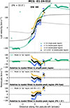 |
Fig. 10. Distribution of the LOS velocity versus the distance along the global kinematic major axis (PA = 32.0°, inside a 0.27″ slit width) of MCG -01-24-012. Values in the single-peak region are shown as blueish-green circles (component c1), while values in the double-peak region are shown as blue (for c1) and orange circles (for c2). The black circles correspond to the average between the LoS velocities of both components (vrot, CND). In the top row, along with the LoS velocity values of each component, we show lines representing models fit to the data. The global disk model, obtained in the single-peak region (see Fig. 7), is shown as a blueish-green line, with the residual shown in the second row. We show two models fit in the CND region (see maps in Fig. F.2, and schematic models in Fig. 11): one with the a free PA parameter (black dashed line, with the residuals in the third row); and another with PA = 0° fixed (black dotted line, with the residuals in the forth row).
|
We can approximately isolate the contribution from the rotation in the double-peak region by averaging the LoS velocities of both components: vrot, CND ∼ (vc1+vc2)/2 (black circles in Fig. 10). Assuming that vrot, CND traces the velocity of the rotation kinematics of the CND, we modeled it using a disk model from Bertola et al. (1991). More specifically, we fit vrot, CND in the double-peak region. The kinematic center was fixed again in the millimeter continuum peak, and the systemic velocity was fixed at the value obtained in the fit done for the single-peak region. The best-fit parameters correspond to a face-on disk geometry (i ∼ 3°). The fourth row of Table 2 displays the parameter values, with Fig. F.2 (first row) showing the corresponding maps.
We observe that this face-on rotating disk model better reproduces the vrot, CND curve compared with the model fit in the single-peak regions, as highlighted by their model residuals Fig. 10 (second and third panels). We sketched a possible scenario for such disk geometry in the first row of Fig. 11: gas previously rotating is disturbed by an ionized outflow, with the energy propagating along this disk (in the north-south direction) and making the CO gas in the CND expand in all directions. The double-peak profile would arise from the simultaneous observation of clumps in the front (with a negative velocity gain in vc1) and the back side of the disk (with positive gain in vc2) (see the lateral view on upper the right panel in Fig. 11).
Nonetheless, it is unclear how a face-on disk could produce the observed CO central flux distribution, which extends along the north-south direction. Additionally, the resulting maximum velocity of the rotation model is unreasonably high: Vmax ∼ 2300 km s−1 (see Table 2). In the last row of Fig. 11 we show another geometry for the CND that could explain the CO flux distribution and the double-peak profiles: an edge-on disk, containing originally rotating molecular clouds, that are outflowing radially – along the CND – due to an almost perpendicular ionized outflow. However, forcing an edge-on disk geometry for the disk (i ∼ 90° and PA ∼ 0°) resulted in a poor fit.
Therefore, we re-fit the data, but fixing only PA at 0°, to better reproduce the CO flux distribution in the CND region. The fit returned an intermediate scenario with an inclination of i = 74 ± 2°. This time, the maximum velocity was lower: Vmax = 270 ± 40 km s−1. Since we fixed PA, the residuals are worse than the model with free PA. The corresponding maps are shown in Fig. F.2 (bottom row), while Fig. 10 shows its velocity radial plot (dotted black line) with the residual of each model being displayed in the last three rows. Since the residuals are more or less aligned with the stellar bar, we question if this stellar structure might also influence the gas in the CND, but we could not answer this with the current data. We point out that the Vmax value is of the order of the maximum velocity found for the CND in NGC 1068, another barred Seyfert galaxy with a previously identified CND (García-Burillo et al. 2019), supporting a similar scenario in MCG -01-012-24.
We conclude that this latter geometry – with PA ∼ 0° and i ∼ 74° (middle row in Fig. 11) – is the best scenario for our observational constraints, as it both produces a rotation curve typical of CNDs and can also explain the flux distribution of the CO emission which is elongated along the north-south direction. Finally, although the CND could be fueling the AGN, we did not find clear evidence of it with current observations, except for the fact that the CND is approximately perpendicular to the ionized gas outflow, as expected for accreting structures around SMBH.
Based on the CND model fit in the double-peak region, we proposed that the CO-emitting gas in the double-peak region was disturbed and partly pushed to the side by the passage of the [O III] ionized outflow, while keeping its bulk rotation motion. This interpretation is consistent with optical, near-infrared, and millimeter observations that report similar line profiles – associated with higher velocity dispersions – in regions outside/perpendicular to the AGN ionization cones and/or radio jets. This has been observed both in the ionized gas (e.g., Venturi et al. 2021; Riffel et al. 2021; Finlez et al. 2018; Lena et al. 2015; Riffel et al. 2014; Couto et al. 2013; Finlez et al. 2018), as well as in both warm (e.g., Riffel et al. 2015; Diniz et al. 2015) and cold molecular gas (e.g., Ramos Almeida et al. 2022; Shimizu et al. 2019; Finlez et al. 2018). Arguing in favor of this scenario, we note that MCG -01-24-012 also presents an elongated radio emission (although barely resolved), almost aligned with the [O III] emission. However, this is only weak evidence of a radio jet. Higher-resolution radio observations are needed to confirm it.
In the CND scenario, the total disturbed molecular mass obtained from CO is Mmol ∼ 3–20 × 107 M⊙, which corresponds to ∼30% of the total cold molecular mass. Assuming an outflow close to the CND plane (i = 74°), the cold molecular mass outflow rate is Ṁmol,out ∼ 0.4–3 M⊙ yr−1. For an different inclination of i = 85° (i = 60°), the Ṁmol,in value would decrease (increase) by a factor of ∼3.3 (∼2.0). We used a de-projected outflow velocity and radius of Vout ∼ 40 km s−1 and Rout ∼ 3 kpc, respectively. See Appendix E.2, for details on the calculation.
9. Discussion: Inflows and outflows
NGC 6860, Mrk 915, and NGC 6860 are part of a larger AGN sample of 13 nearby sources observed with ALMA, as described in Paper I. Analogously to our three objects, in the other ten objects, the bulk of the CO gas is rotating in a disk, with all of them displaying local non-circular motions within a few kiloparsecs (Ramakrishnan et al. 2019; Slater et al. 2019; Finlez et al. 2018; Salvestrini et al. 2020; Dall’Agnol de Oliveira et al. 2023), which could be expected since they were selected for having signs of disturbance in the ionized gas. In our three Seyfert galaxies, the disturbances seem to be related to inflows and outflows in the cold molecular gas, and to the presence of circumnuclear disks.
9.1. Inflows
There is evidence of CO molecular inflows along a bar in NGC 6860 and along a spiral arm in Mrk 915. However, for Mrk 915, the inflow interpretation is only true if we assume a leading spiral arm scenario. Otherwise, it would be consistent with outflows. In these two sources, we might be witnessing the processes responsible for driving material to nuclear regions, which end up feeding the AGN. However, the relative importance of different mechanisms in the feeding process is still debatable. Here, we focus on stellar structures associated with inflows in our sources. We refer to Storchi-Bergmann & Schnorr-Müller (2019) for a review on the subject.
Stellar bars – as in NGC 6860 – have long been proposed to play a significant role in feeding AGN activity and also nuclear star formation (e.g., Shlosman et al. 1989). A few studies claim that AGN are more frequently found in barred systems (e.g., Silva-Lima et al. 2022; Alonso et al. 2013), although the majority seem to discard this hypothesis (e.g., Cheung et al. 2015; Erwin & Sparke 2002; Ho et al. 1997).
Spiral arms – as in Mrk 915 – have been predicted to help drive gas to the central kiloparsec (e.g., Kim et al. 2014), with evidence of higher molecular gas concentration in galaxies with more prominent spirals (e.g., Yu et al. 2022). At smaller scales, ∼10–100 pc, there are plenty of examples of inflows along nuclear spirals in AGN (e.g., Bianchin et al. 2024; Riffel et al. 2013, 2008; Storchi-Bergmann et al. 2007).
Additionally, Mrk 915 is part of a triple system with signs of a warped outer disk, evidencing tidal interactions with nearby objects (see Fig. 1). This is one of the several processes that are typically claimed to play a significant role in triggering nuclear activity (e.g., Araujo et al. 2023; Steffen et al. 2023). It is important to note that not all accreted gas ends up feeding the black hole. For example, the new material might lead to local bursts of star formation (König et al. 2014).
We note that the three Seyfert galaxies show quite a degree of variability in X-rays and the BLR emission lines. The observed molecular inflows – in NGC 6860 and possibly in Mrk 915 (depending on the disk orientation) – may be related to this variability. In the sense that episodes of higher accretion rate may both increase the AGN luminosity and partially block the nuclear radiation, leading to a decrease in the luminosity. Nonetheless, the molecular inflows observed in our sample are probably only responsible for transporting material to the inner ∼100 parsec. And, the short timescales of their X-ray variability are probably associated with episodes of intermittent capture of gas clouds flowing into the central regions (Storchi-Bergmann & Schnorr-Müller 2019).
These CO flows translates to measured cold molecular inflow rate values of Ṁmol,in ∼ 0.8–6 M⊙ yr−1 and 0.09–0.8 M⊙ yr−1 for NGC 6860 and Mrk 915, respectively. We can compare this with published values in the literature for different objects, to evaluate if these are typical values or outliers. The AGN/starburst host Fairall 49 shows rising Ṁmol,in values along a bar, reaching ∼ 5 M⊙ yr−1 (Lelli et al. 2022). They note that this value is consistent with the zoom-in cosmological simulations of quasar fueling from Anglés-Alcázar et al. (2021), although the rate can vary significantly, spanning a range of 0.001–10 M⊙ yr−1. Similarly, Wu et al. (2021) found a ∼ 12 M⊙ yr−1 inflow rate in NGC 3504 along the bar’s dust lanes. In NGC 1365, the inflow rates grow from ∼6 M⊙ yr−1 in the spirals arms to ∼40 M⊙ yr−1 in the bar (Elmegreen et al. 2009). And, in a sample of seven spiral galaxies, most of them barred, Haan et al. (2009) observed inflow rates of ∼0.01–50 M⊙ yr−1. Overall, the inflow rates from our sources do not seem to stand out.
9.2. Outflows
The three Seyfert galaxies show signs of AGN-induced disturbances in the cold molecular gas, but with their own characteristics. In NGC 6860, the CO outflowing clouds seem to surround an [O III] ionized gas outflow. In Mrk 915, the outflow is observed along one of the spirals, although its presence depends on the disk orientation (scenario of trailing spiral arms). In MCG -01-24-012, the disturbance in the CO gas is observed perpendicular to the projected ionization axis, indicating that it propagates equatorially.
The difference in how the molecular gas is disturbed might be a consequence of different ionization axis inclinations relative to the disk (Harrison & Ramos Almeida 2024). Larger angles between the winds and/or jets axes relative to the galaxy disk result in a weaker coupling between the released energy and the gas in the disk (Mukherjee et al. 2018). This is, for example, our proposed scenario for MCG -01-24-012 (see Fig. 1), which might help explain why the spatial anticorrelation between CO and [O III] is less pronounced in this source, when compared with our other two Seyfert galaxies (Paper I). We note that the above considerations might not fully apply if the molecular gas originally lies above the disk.
In NGC 6860 and Mrk 915, only fout ∼ 0.7–4% of the gas (in mass) is outflowing. In MCG -01-24-012, a higher fraction of ∼30% seems to be disturbed, although the bulk kinematics of the gas in this region follows an ordered motion of rotating in a disk, and the outflow velocity is only Vout ∼ 40 km s−1. The corresponding mass outflow rates of our sources are in the range of Ṁmol,out ∼ 0.09–3 M⊙ yr−1. Overall, the Ṁmol,out, fout and outflow velocity (Vout ∼ 40–300 km s−1) values seems to indicate relatively weak AGN feedback on the cold molecular gas. However, as discussed in Paper I, part of the molecular gas is likely being depleted by the energy released by the AGN on the ISM. This information is not covered by Ṁmol,out measurements, although it could also be considered a type of negative feedback.
We can compare Ṁmol,out from our sources with published values from resolved outflow observations. We can divide the reported Ṁmol,out measurements in the literature into two classes: weak/moderate cold molecular outflow, in the range Ṁmol,out ∼ 0.1–10 M⊙ yr−1 (e.g., Oosterloo et al. 2017; Slater et al. 2019; Alonso-Herrero et al. 2019; Dall’Agnol de Oliveira et al. 2023); and strong outflows, with values of 10–102 M⊙ yr−1 (e.g., García-Burillo et al. 2014; Alonso Herrero et al. 2023; García-Bernete et al. 2021; Audibert et al. 2019). Our sample is closer to the first class of weak cold molecular outflows. A broader compilation of Ṁout,mol measurements from the literature, covering 5–6 orders of magnitude in LAGN, have been made by Alonso Herrero et al. (2023, see their Fig. 13)2, showing a positive trend between both quantities. In this compilation, there are about eight objects in the same range of luminosities of our three Seyfert galaxies: LAGN ∼ 1043.6–1044.8 erg s−1. All of the eight objects have Ṁout,mol values higher than our three sources, by factors of ∼2–100 (compared with our maximum value of 3 M⊙ yr−1). This indicates that the AGN feedback in NGC 6860, Mrk 915, and MCG -01-24-012 might be particularly weak, if we assume that our values are not underestimated, or the opposite for the literature values. However, this is only an exploratory comparison. A more comprehensive comparison should consider uncertainties in the measurements of other authors and try to homogenize the methods used to calculate the mass outflow rates, which are know to vary a lot (e.g., Harrison et al. 2018; Dall’Agnol de Oliveira et al. 2021). Such analysis is beyond the scope of this work. In Section 9.4, we list some sources of uncertainties in our measurements.
9.3. Comparing different flow rates
We can compare the measured Ṁmol,in with the mass accretion rates required to feed the AGN Ṁacc = LAGN/(c2 η). By assuming an efficiency of conversion of accreted matter into radiation of η = 0.1 (Frank et al. 2002), and using the mean LAGN value from Table 1, we obtain Ṁacc values of ∼0.009, ∼0.03, and ∼0.07 M⊙ yr−1, for NGC 6860, Mrk 915, and MCG -01-24-012, respectively, with a 0.2 dex uncertainty (from the range in the LAGN values). Focusing on the sources inflows detections, we obtain ratios of Ṁmol,in/Ṁacc ∼ 70–850 (for NGC 6860) and 3–40 times (for Mrk 915, in the leading arms scenario). Hence, the mass inflow rate is larger than the rate required to power the current AGN event in each object. It is important to note that comparing Ṁmol,in, at scales of hundreds parsecs, with Ṁacc, which happens at parsec scales, is not straightforward. The mechanisms involved in driving gas to nuclear regions, leading to a new AGN event, are probably episodic and occur at different timescales compared to larger-scale inflows (Storchi-Bergmann & Schnorr-Müller 2019)
We can also compare the mass accretion rate and the molecular outflow rates. We obtained ratio values of Ṁmol,out/Ṁacc ∼ 9–140, 3–30, and 4–90, for NGC 6860, Mrk 915 (in the trailing arms scenario), and MCG -01-24-012, respectively. The accretion rate being lower than the mass outflow rate is in qualitative agreement with what has been observed for the ionized and hot molecular gas (e.g., Müller-Sánchez et al. 2011; Bianchin et al. 2022; Barbosa et al. 2009; Riffel & Storchi-Bergmann 2011; Schnorr-Müller et al. 2014). If we assume that the AGN feedback is only responsible for the observed disturbances in the CO, this suggests that only a fraction of the outflowing clouds are launched directly by the energy released by the AGN. The remaining outflowing gas might originate from the surrounding ISM, which could have been disturbed and pushed away in the past by the AGN events. Moreover, part of the ejected molecular gas could have been driven by local starbursts. We note, however, that there are no clear signs of a young stellar population close to the disturbed regions in NGC 6860 (Lipari et al. 1993; Bennert et al. 2006) and in Mrk 915 (Trippe et al. 2010; Bennert et al. 2006), as judged from emission line ratios and optical continuum. Mrk 915 seems to have an excess of UV continuum emission, which could be a hint of a nuclear starburst (Muñoz Marín et al. 2009), but a careful modeling of the UV continuum is needed to discard other contributions, such as the AGN continuum, scattered light, and nebular emission. For MCG -01-24-012, we did not find external evidence in favor (or not) of ongoing star formation in the double-peak CO region.
Finally, we can compare the mass inflow and outflow rates. For Mrk 915, the inflow and outflow scenarios are mutually exclusive, making a comparison between them not possible. We therefore only focus on NGC 6860, where the ratio between these values is Ṁmol,out/Ṁmol,in ∼ 0.1. When comparing all the flow rates, we found that ṀaccṀmol,out ≲ Ṁmol,in in this source. Analogously to the comparison between Ṁmol,in and Ṁacc, comparing the Ṁmol,out and Ṁmol,in is not straightforward due to different spatial and temporal scales involved. If we ignore that, the above ratio suggests that part of the infalling CO clouds might be ejected and/or disturbed by the AGN feedback before reaching the nuclear region. We note that this considers only the cold molecular phase traced by CO(2-1) and the impact on it associated with the AGN feedback.
The above discussions raise the question of whether the inflowing cold molecular gas leads to an accumulation of a nuclear reservoir of molecular gas. Besides the fraction that is observed in outflow, part of it might be depleted by the ionized outflow, jets, and/or radiation, as suggested by spatial anticorrelation between CO and the [O III] ionized gas emission within the inner kiloparsec region of these two sources (Dall’Agnol de Oliveira et al. 2025). We believe that we are observing a scenario analogous to the results obtained by García-Burillo et al. (2024). They found evidence that the molecular reservoir builds up over time in the central regions, with higher molecular gas concentrations being observed in more luminous AGN, probably a consequence of higher AGN mass accretion rates. For objects with X-ray luminosities above ∼1041.5 erg s−1 – as our sources – the negative AGN feedback starts to affect the molecular gas nuclear reservoir, decreasing the nuclear concentration. In addition, part of the extra fuel can also be used to form new stars. However, as discussed above, we did not find strong evidence for ongoing nuclear star formation.
9.4. Caveats
Here we list some caveats of our results. Probably the highest source of uncertainty for mass-related measurements is the r21 and αCO factors, used to convert the CO(2-1) flux to H2 masses (see Appendix E, for details), and for which we do not have direct measurements for our sources. Together, the wide range of r21 = 0.8–1.2 and αCO = 0.8–4.3 M⊙ [K km s−1 pc−2]−1 values used in this work introduce an order-of-magnitude uncertainty in molecular mass values. We choose to use such ranges because they cover different physical scenarios. In particular for outflowing CO clouds, αCO values closer to our minimum range have been used in the literature (e.g., Morganti et al. 2015; Dasyra et al. 2016; Ramos Almeida et al. 2022). In addition, direct measurements, using CO rovibrational infrared lines, indicate that the αCO might be even smaller by a factor of up to ∼2 (Pereira-Santaella et al. 2024). In such a case, when dealing with the values presented in this work, one should consider the lower values of the Mmol, out and Ṁmol,out ranges as more reliable measurements.
For simplicity, we assumed that both the inflows and outflows occur at the same plane, with an inclination obtained for the gas rotating in a disk. However, when inflowing and outflowing CO clouds are observed along the same LoS, it is reasonable to suspect that the outflow occurs outside the disk plane. For example, assuming an outflow above the disk in NGC 6860 (inclination > 57.7°), would increase the resulting Rout values while decreasing Vout and Ṁmol,out. By varying the inclinations by Δi ∼ 10–15°, we showed that values of Ṁmol,out (and Ṁmol,in) can vary by a factor of up to ∼3 (see Sects. 6.2.1, 6.3, 7.2.1 and 8.2).
Another source of uncertainty is the definition of outflow velocity, here we calculated from the LoS velocity residuals of the CO component tracing the outflow. Other authors have used different definitions that return higher values of Vout (e.g., Sun et al. 2017; Karouzos et al. 2016; Bischetti et al. 2019). For example, using Vout = v + 2 σ increases Mmol, out by a factor of up to ∼3 in our sources, which is still within the uncertainty associated with the mass. We refer to Harrison et al. (2018), Harrison & Ramos Almeida (2024) for a broader discussion on the different methods and assumptions, such as the outflow geometry, which one can use to calculate mass outflow rates.
Inflows and outflows were identified based on the residuals of the 2D rotating disk models. We tested different scenarios in NGC 6860 and MCG -01-24-012, and we considered the two possible disk orientations for Mrk 915. However, from our analysis, we cannot discard that more complex models might lead to different interpretations of the results.
10. Conclusions
We have analyzed the cold molecular gas distribution and kinematics – as traced by CO(2-1) – in three local Seyfert galaxies observed with ALMA. The high angular resolution of the ALMA observations allowed us to resolve the gas on scales of ∼0.5–0.8″ (∼150–400 pc). Below, we summarize the picture drawn for each object.
10.1. NGC 6860.
The CO emission is observed along a stellar ring and its internal stellar bar. Along the ring, the molecular gas mostly follows the disk rotation. We discussed two scenarios for CO in the bar: a molecular gas inflow along the bar with an inflow rate of Ṁmol,in ∼ 0.8–6 M⊙ yr−1 and a decoupled CND rotating in a different plane from that of the gas in the ring. There is also a molecular gas outflow within Rout ∼ 560 pc from the nucleus surrounding part of the bipolar [O III] ionization cone and outflow and with a mass outflow rate of Ṁmol,out ∼ 0.1–1 M⊙ yr−1.
10.2. Mrk 915.
The cold molecular gas mostly lies along spiral arms, with rotation dominating the kinematics. There is a region with CO double-peak profiles along one of the spiral arms, indicating the presence of two kinematic components. Due to the uncertain orientation of the galaxy’s disk, one of the components could either be tracing an inflowing stream of molecular gas or an outflow, with the galaxy having leading or trailing spiral arms, respectively. In the hypothesis of inflows, the mass inflow rate would be Ṁmol,in ∼ 0.09–0.8 M⊙ yr−1, while in the case of outflow, the mass outflow rate would be Ṁmol,out ∼ 0.09–0.7 M⊙ yr−1 with Rout ∼ 2.8 kpc. The influence of nearby galaxies might play a role in both scenarios. We note that the lower S/N of Mrk 915’s spectra might affect our conclusions. Deeper observations are needed to better model its kinematics.
10.3. MCG -01-24-012.
The cold molecular gas is partly located along a ∼3 kpc (radius) stellar ring, with kinematics dominated by rotation. The CO emission is also observed inside the ring, including along the stellar bar. In the inner kiloparsecs, the CO emission extends almost perpendicularly to the [O III] ionization cone, with an orientation distinct from the outer galaxy disk. We identify this region as a possible CND, with molecular gas outflowing along it, although the kinematics are still dominated by rotation. This effect is probably caused by an ionized gas outflow associated with the bipolar [O III] emission that disturbs the molecular gas and produces an equatorial outflow with Ṁmol,in ∼ 0.4–3 M⊙ yr−1 and Rout ∼ 3 kpc.
Analyzing the results of the three Seyfert galaxies together, we found the following common features:
-
The bulk of the molecular gas rotates in the galaxy disk near stellar structures identified as bars, rings, and spirals. Within ∼0.56–3 kpc, we found disturbances in the molecular gas, as traced by CO double-peak spectral profiles. We showed that these disturbances are associated with CO inflows and outflows and that the gas might be rotating in a different plane as part of a CND, as in the case of MCG -01-24-012 and possibly in NGC 6860.
-
The mass outflow rates are in the range Ṁmol,out ∼ 0.09–3 M⊙ yr−1. This suggests a particular weak negative AGN feedback in the cold molecular gas when compared with other sources with similar AGN luminosities, LAGN ∼ 1044 erg s−1( Ṁmol,out values larger by factors of ∼2–100).
-
Only a fraction of the inflowing molecular clouds ends up feeding the AGN since the inflow rates of NGC 6860 and Mrk 915 (in the trailing arms scenario) are approximately 3–850 times the AGN mass accretion rate.
-
The AGN accretion rate is also not enough to feed the observed CO outflow mass rates, as they are lower by factors of about 3–140. This indicates that the mass outflow rate is due to mass loading of nuclear outflows from molecular gas that has accumulated over time in the circumnuclear region. There is also a possible contribution of nuclear starbursts, although we did not find clear evidence of it in our sources.
Although the measured Ṁmol,out indicates a weak impact in this gas phase, the presence of regions with a CO deficit in our three sources suggests that the AGN feedback might be depleting part of the molecular gas content (Paper I). This is an impact that is not taken into account by Ṁmol,out, but it should receive more attention in future works. In agreement with results from García-Burillo et al. (2024), our sources might be increasing the CO reservoir close to the nucleus, given the measured inflow rates. This buildup then leads to an increase in the AGN mass accretion rate, which increases the AGN total energy output. Given the current AGN luminosity, we might be observing the beginning of the depletion of the nuclear molecular reservoir in our sources.
Approximate values, collected from Fig. 7 of Lipari et al. (1993), using PlotDigitizer: https://plotdigitizer.com
Data from NGC 7172, measured in that work, and Lutz et al. (2020), García-Burillo et al. (2014), Ramos Almeida et al. (2022), Lamperti et al. (2022).
Acknowledgments
This study was financed in part by the Coordenação de Aperfeiçoamento de Pessoal de Nível Superior (CAPES-Brasil, 88887.478902/2020-00, 88887.985730/2024-00). RAR acknowledges the support from Conselho Nacional de Desenvolvimento Científico e Tecnológico (CNPq; Proj. 303450/2022-3, 403398/2023-1, & 441722/2023-7), Fundação de Amparo à pesquisa do Estado do Rio Grande do Sul (FAPERGS; Proj. 21/2551-0002018-0), and CAPES (Proj. 88887.894973/2023-00). This paper makes use of the following ALMA data: ADS/JAO.ALMA#2018.1.00211.S. ALMA is a partnership of ESO (representing its member states), NSF (USA) and NINS (Japan), together with NRC (Canada), MOST and ASIAA (Taiwan), and KASI (Republic of Korea), in cooperation with the Republic of Chile. The Joint ALMA Observatory is operated by ESO, AUI/NRAO and NAOJ. The Legacy Surveys consist of three individual and complementary projects: the Dark Energy Camera Legacy Survey (DECaLS; Proposal ID #2014B-0404; PIs: David Schlegel and Arjun Dey), the Beijing-Arizona Sky Survey (BASS; NOAO Prop. ID #2015A-0801; PIs: Zhou Xu and Xiaohui Fan), and the Mayall z-band Legacy Survey (MzLS; Prop. ID #2016A-0453; PI: Arjun Dey). DECaLS, BASS and MzLS together include data obtained, respectively, at the Blanco telescope, Cerro Tololo Inter-American Observatory, NSF’s NOIRLab; the Bok telescope, Steward Observatory, University of Arizona; and the Mayall telescope, Kitt Peak National Observatory, NOIRLab. Pipeline processing and analyzes of the data were supported by NOIRLab and the Lawrence Berkeley National Laboratory (LBNL). The Legacy Surveys project is honored to be permitted to conduct astronomical research on Iolkam Du’ag (Kitt Peak), a mountain with particular significance to the Tohono O’odham Nation. This research has made use of the NASA/IPAC Extragalactic Database, which is funded by the National Aeronautics and Space Administration and operated by the California Institute of Technology. This work used the color scheme from Wong (2011) in some of the plots to minimize confusion for colorblind viewers. Figure 8 was generated by combining the following software: FREECAD, LIBREOFFICE DRAW and MATPLOTLIB.
References
- Alonso Herrero, A., García-Burillo, S., Pereira-Santaella, M., et al. 2023, A&A, 675, A88 [NASA ADS] [CrossRef] [EDP Sciences] [Google Scholar]
- Alonso, M. S., Coldwell, G., & Lambas, D. G. 2013, A&A, 549, A141 [NASA ADS] [CrossRef] [EDP Sciences] [Google Scholar]
- Alonso-Herrero, A., García-Burillo, S., Pereira-Santaella, M., et al. 2019, A&A, 628, A65 [NASA ADS] [CrossRef] [EDP Sciences] [Google Scholar]
- Anglés-Alcázar, D., Quataert, E., Hopkins, P. F., et al. 2021, ApJ, 917, 53 [CrossRef] [Google Scholar]
- Araujo, B. L. C., Storchi-Bergmann, T., Rembold, S. B., Kaipper, A. L. P., & Dall’Agnol de Oliveira, B. 2023, MNRAS, 522, 5165 [NASA ADS] [CrossRef] [Google Scholar]
- Audibert, A., Combes, F., García-Burillo, S., et al. 2019, A&A, 632, A33 [NASA ADS] [CrossRef] [EDP Sciences] [Google Scholar]
- Ballo, L., Severgnini, P., Della Ceca, R., et al. 2017, MNRAS, 470, 3924 [Google Scholar]
- Barbosa, F. K. B., Storchi-Bergmann, T., Cid Fernandes, R., Winge, C., & Schmitt, H. 2009, MNRAS, 396, 2 [Google Scholar]
- Bennert, N., Jungwiert, B., Komossa, S., Haas, M., & Chini, R. 2006, A&A, 459, 55 [NASA ADS] [CrossRef] [EDP Sciences] [Google Scholar]
- Bertola, F., Bettoni, D., Danziger, J., et al. 1991, ApJ, 373, 369 [Google Scholar]
- Bianchin, M., Riffel, R. A., Storchi-Bergmann, T., et al. 2022, MNRAS, 510, 639 [Google Scholar]
- Bianchin, M., U, V., Song, Y., et al. 2024, ApJ, 965, 103 [NASA ADS] [CrossRef] [Google Scholar]
- Bischetti, M., Maiolino, R., Carniani, S., et al. 2019, A&A, 630, A59 [NASA ADS] [CrossRef] [EDP Sciences] [Google Scholar]
- Bolatto, A. D., Warren, S. R., Leroy, A. K., et al. 2013a, Nature, 499, 450 [Google Scholar]
- Bolatto, A. D., Wolfire, M., & Leroy, A. K. 2013b, ARA&A, 51, 207 [CrossRef] [Google Scholar]
- Braine, J., & Combes, F. 1992, A&A, 264, 433 [NASA ADS] [Google Scholar]
- Byrd, G. G., Freeman, T., & Howard, S. 1993, AJ, 105, 477 [NASA ADS] [CrossRef] [Google Scholar]
- Byrd, G. G., Freeman, T., Howard, S., & Buta, R. J. 2008, AJ, 135, 408 [Google Scholar]
- Cheung, E., Trump, J. R., Athanassoula, E., et al. 2015, MNRAS, 447, 506 [NASA ADS] [CrossRef] [Google Scholar]
- Cicone, C., Maiolino, R., Sturm, E., et al. 2014, A&A, 562, A21 [NASA ADS] [CrossRef] [EDP Sciences] [Google Scholar]
- Cicone, C., Brusa, M., Ramos Almeida, C., et al. 2018, Nat. Astron., 2, 176 [Google Scholar]
- Couto, G. S., Storchi-Bergmann, T., Axon, D. J., et al. 2013, MNRAS, 435, 2982 [Google Scholar]
- Dall’Agnol de Oliveira, B., Storchi-Bergmann, T., Kraemer, S. B., et al. 2021, MNRAS, 504, 3890 [CrossRef] [Google Scholar]
- Dall’Agnol de Oliveira, B., Storchi-Bergmann, T., Morganti, R., Riffel, R. A., & Ramakrishnan, V. 2023, MNRAS, 522, 3753 [CrossRef] [Google Scholar]
- Dall’Agnol de Oliveira, B., Storchi-Bergmann, T., Nagar, N., et al. 2025, A&A, 701, A48 [NASA ADS] [CrossRef] [EDP Sciences] [Google Scholar]
- Dasyra, K. M., Combes, F., Oosterloo, T., et al. 2016, A&A, 595, L7 [NASA ADS] [CrossRef] [EDP Sciences] [Google Scholar]
- de Vaucouleurs, G. 1958, ApJ, 127, 487 [Google Scholar]
- de Vaucouleurs, G., de Vaucouleurs, A., Corwin, H. G. J., et al. 1991, Third Reference Catalogue of Bright Galaxies (New York: Springer) [Google Scholar]
- Delabrosse, V., Dougados, C., Cabrit, S., et al. 2024, A&A, 688, A173 [NASA ADS] [CrossRef] [EDP Sciences] [Google Scholar]
- Di Teodoro, E. M., & Fraternali, F. 2015, MNRAS, 451, 3021 [Google Scholar]
- Diniz, M. R., Riffel, R. A., Storchi-Bergmann, T., & Winge, C. 2015, MNRAS, 453, 1727 [Google Scholar]
- Elmegreen, B. G., Galliano, E., & Alloin, D. 2009, ApJ, 703, 1297 [Google Scholar]
- Erwin, P., & Sparke, L. S. 2002, AJ, 124, 65 [Google Scholar]
- Evans, N. W., & Read, J. C. A. 1998, MNRAS, 300, 106 [Google Scholar]
- Feruglio, C., Maiolino, R., Piconcelli, E., et al. 2010, A&A, 518, L155 [NASA ADS] [CrossRef] [EDP Sciences] [Google Scholar]
- Finlez, C., Nagar, N. M., Storchi-Bergmann, T., et al. 2018, MNRAS, 479, 3892 [Google Scholar]
- Frank, J., King, A., & Raine, D. J. 2002, Accretion Power in Astrophysics, 3rd edn. (UK: Cambridge University Press) [Google Scholar]
- Gallagher, R., Maiolino, R., Belfiore, F., et al. 2019, MNRAS, 485, 3409 [NASA ADS] [CrossRef] [Google Scholar]
- García-Bernete, I., Alonso-Herrero, A., García-Burillo, S., et al. 2021, A&A, 645, A21 [EDP Sciences] [Google Scholar]
- García-Burillo, S., Sempere, M. J., Combes, F., Hunt, L. K., & Neri, R. 2000, A&A, 363, 869 [Google Scholar]
- García-Burillo, S., Combes, F., Hunt, L. K., et al. 2003, A&A, 407, 485 [NASA ADS] [CrossRef] [EDP Sciences] [Google Scholar]
- García-Burillo, S., Combes, F., Usero, A., et al. 2014, A&A, 567, A125 [Google Scholar]
- García-Burillo, S., Combes, F., Ramos Almeida, C., et al. 2019, A&A, 632, A61 [Google Scholar]
- García-Burillo, S., Hicks, E. K. S., Alonso-Herrero, A., et al. 2024, A&A, 689, A347 [NASA ADS] [CrossRef] [EDP Sciences] [Google Scholar]
- Goodrich, R. W. 1995, ApJ, 440, 141 [CrossRef] [Google Scholar]
- Grouchy, R. D., Buta, R., Salo, H., Laurikainen, E., & Speltincx, T. 2008, AJ, 136, 980 [NASA ADS] [CrossRef] [Google Scholar]
- Haan, S., Schinnerer, E., Emsellem, E., et al. 2009, ApJ, 692, 1623 [NASA ADS] [CrossRef] [Google Scholar]
- Harrison, C. M., & Ramos Almeida, C. 2024, Galaxies, 12, 17 [NASA ADS] [CrossRef] [Google Scholar]
- Harrison, C. M., Costa, T., Tadhunter, C. N., et al. 2018, Nat. Astron., 2, 198 [Google Scholar]
- Heckman, T. M., & Best, P. N. 2014, ARA&A, 52, 589 [Google Scholar]
- Hicks, E. K. S., Davies, R. I., Malkan, M. A., et al. 2009, ApJ, 696, 448 [NASA ADS] [CrossRef] [Google Scholar]
- Ho, L. C., Filippenko, A. V., & Sargent, W. L. W. 1997, ApJ, 487, 591 [NASA ADS] [CrossRef] [Google Scholar]
- Iye, M., Tadaki, K.-I., & Fukumoto, H. 2019, ApJ, 886, 133 [Google Scholar]
- Karachentseva, V. E., & Karachentsev, I. D. 2000, Astron. Rep., 44, 501 [NASA ADS] [CrossRef] [Google Scholar]
- Karouzos, M., Woo, J.-H., & Bae, H.-J. 2016, ApJ, 819, 148 [NASA ADS] [CrossRef] [Google Scholar]
- Khoperskov, S., Haywood, M., Di Matteo, P., Lehnert, M. D., & Combes, F. 2018, A&A, 609, A60 [NASA ADS] [CrossRef] [EDP Sciences] [Google Scholar]
- Kim, W.-T., Kim, Y., & Kim, J.-G. 2014, ApJ, 789, 68 [NASA ADS] [CrossRef] [Google Scholar]
- König, S., Aalto, S., Muller, S., Beswick, R. J., & Gallagher, J. S. 2013, A&A, 553, A72 [NASA ADS] [CrossRef] [EDP Sciences] [Google Scholar]
- König, S., Aalto, S., Lindroos, L., et al. 2014, A&A, 569, A6 [NASA ADS] [CrossRef] [EDP Sciences] [Google Scholar]
- La Franca, F., Onori, F., Ricci, F., et al. 2015, MNRAS, 449, 1526 [Google Scholar]
- Lamperti, I., Pereira-Santaella, M., Perna, M., et al. 2022, A&A, 668, A45 [NASA ADS] [CrossRef] [EDP Sciences] [Google Scholar]
- Lelli, F., Davis, T. A., Bureau, M., et al. 2022, MNRAS, 516, 4066 [NASA ADS] [CrossRef] [Google Scholar]
- Lena, D., Robinson, A., Storchi-Bergman, T., et al. 2015, ApJ, 806, 84 [Google Scholar]
- Lenz, D. D., & Ayres, T. R. 1992, PASP, 104, 1104 [NASA ADS] [CrossRef] [Google Scholar]
- Levy, R. C., Bolatto, A. D., Teuben, P., et al. 2018, ApJ, 860, 92 [NASA ADS] [CrossRef] [Google Scholar]
- Lieb, E., Collier, A., & Madigan, A.-M. 2022, MNRAS, 509, 685 [Google Scholar]
- Lipari, S., Tsvetanov, Z., & Macchetto, F. 1993, ApJ, 405, 186 [Google Scholar]
- Luo, G., Zhang, Z.-Y., Bisbas, T. G., et al. 2023, ApJ, 946, 91 [NASA ADS] [CrossRef] [Google Scholar]
- Lutz, D., Sturm, E., Janssen, A., et al. 2020, A&A, 633, A134 [NASA ADS] [CrossRef] [EDP Sciences] [Google Scholar]
- Maiolino, R., Russell, H. R., Fabian, A. C., et al. 2017, Nature, 544, 202 [Google Scholar]
- Malizia, A., Malaguti, G., Bassani, L., et al. 2002, A&A, 394, 801 [NASA ADS] [CrossRef] [EDP Sciences] [Google Scholar]
- Malkan, M. A., Gorjian, V., & Tam, R. 1998, ApJS, 117, 25 [Google Scholar]
- Matt, G., Guainazzi, M., & Maiolino, R. 2003, MNRAS, 342, 422 [NASA ADS] [CrossRef] [Google Scholar]
- Mezcua, M., Prieto, M. A., Fernández-Ontiveros, J. A., et al. 2015, MNRAS, 452, 4128 [NASA ADS] [CrossRef] [Google Scholar]
- Middei, R., Matzeu, G. A., Bianchi, S., et al. 2021, A&A, 647, A102 [NASA ADS] [CrossRef] [EDP Sciences] [Google Scholar]
- Morganti, R., Oosterloo, T., Oonk, J. B. R., Frieswijk, W., & Tadhunter, C. 2015, A&A, 580, A1 [NASA ADS] [CrossRef] [EDP Sciences] [Google Scholar]
- Morganti, R., Murthy, S., Guillard, P., Oosterloo, T., & Garcia-Burillo, S. 2023, Galaxies, 11, 24 [NASA ADS] [CrossRef] [Google Scholar]
- Mukherjee, D., Bicknell, G. V., Wagner, A. Y., Sutherland, R. S., & Silk, J. 2018, MNRAS, 479, 5544 [NASA ADS] [CrossRef] [Google Scholar]
- Müller-Sánchez, F., Prieto, M. A., Hicks, E. K. S., et al. 2011, ApJ, 739, 69 [Google Scholar]
- Muñoz Marín, V. M., Storchi-Bergmann, T., González Delgado, R. M., et al. 2009, MNRAS, 399, 842 [Google Scholar]
- Nagar, N. M., Vogel, S. N., Stone, J. M., & Ostriker, E. C. 1997, ApJ, 482, L195 [Google Scholar]
- Onori, F., La Franca, F., Ricci, F., et al. 2017, MNRAS, 464, 1783 [NASA ADS] [CrossRef] [Google Scholar]
- Oosterloo, T., Raymond Oonk, J. B., Morganti, R., et al. 2017, A&A, 608, A38 [NASA ADS] [CrossRef] [EDP Sciences] [Google Scholar]
- Pereira-Santaella, M., González-Alfonso, E., García-Bernete, I., García-Burillo, S., & Rigopoulou, D. 2024, A&A, 681, A117 [NASA ADS] [CrossRef] [EDP Sciences] [Google Scholar]
- Ramakrishnan, V., Nagar, N. M., Finlez, C., et al. 2019, MNRAS, 487, 444 [Google Scholar]
- Ramos Almeida, C., Bischetti, M., García-Burillo, S., et al. 2022, A&A, 658, A155 [NASA ADS] [CrossRef] [EDP Sciences] [Google Scholar]
- Ricci, F., Treister, E., Bauer, F. E., et al. 2022, ApJS, 261, 8 [NASA ADS] [CrossRef] [Google Scholar]
- Riffel, R. A., & Storchi-Bergmann, T. 2011, MNRAS, 417, 2752 [Google Scholar]
- Riffel, R. A., Storchi-Bergmann, T., Winge, C., et al. 2008, MNRAS, 385, 1129 [CrossRef] [Google Scholar]
- Riffel, R. A., Storchi-Bergmann, T., & Winge, C. 2013, MNRAS, 430, 2249 [Google Scholar]
- Riffel, R. A., Storchi-Bergmann, T., & Riffel, R. 2014, ApJ, 780, L24 [Google Scholar]
- Riffel, R. A., Storchi-Bergmann, T., & Riffel, R. 2015, MNRAS, 451, 3587 [Google Scholar]
- Riffel, R. A., Dors, O. L., Armah, M., et al. 2021, MNRAS, 501, L54 [Google Scholar]
- Ruschel-Dutra, D., Storchi-Bergmann, T., Schnorr-Müller, A., et al. 2021, MNRAS, 507, 74 [NASA ADS] [CrossRef] [Google Scholar]
- Russell, H. R., McDonald, M., McNamara, B. R., et al. 2017, ApJ, 836, 130 [NASA ADS] [CrossRef] [Google Scholar]
- Saintonge, A., & Catinella, B. 2022, ARA&A, 60, 319 [NASA ADS] [CrossRef] [Google Scholar]
- Salvestrini, F., Gruppioni, C., Pozzi, F., et al. 2020, A&A, 641, A151 [NASA ADS] [CrossRef] [EDP Sciences] [Google Scholar]
- Scaloni, L., Rodighiero, G., Enia, A., et al. 2024, A&A, 687, A255 [NASA ADS] [CrossRef] [EDP Sciences] [Google Scholar]
- Schmitt, H. R., & Kinney, A. L. 2000, ApJS, 128, 479 [Google Scholar]
- Schmitt, H. R., Ulvestad, J. S., Antonucci, R. R. J., & Kinney, A. L. 2001, ApJS, 132, 199 [NASA ADS] [CrossRef] [Google Scholar]
- Schmitt, H. R., Donley, J. L., Antonucci, R. R. J., Hutchings, J. B., & Kinney, A. L. 2003, ApJS, 148, 327 [NASA ADS] [CrossRef] [Google Scholar]
- Schnorr-Müller, A., Storchi-Bergmann, T., Nagar, N. M., et al. 2014, MNRAS, 437, 1708 [Google Scholar]
- Sellwood, J. A., & Athanassoula, E. 1986, MNRAS, 221, 195 [NASA ADS] [Google Scholar]
- Serafinelli, R., Severgnini, P., Braito, V., et al. 2020, ApJ, 902, 10 [Google Scholar]
- Severgnini, P., Ballo, L., Braito, V., et al. 2015, MNRAS, 453, 3611 [Google Scholar]
- Shimizu, T. T., Davies, R. I., Lutz, D., et al. 2019, MNRAS, 490, 5860 [Google Scholar]
- Shlosman, I., Frank, J., & Begelman, M. C. 1989, Nature, 338, 45 [Google Scholar]
- Silva-Lima, L. A., Martins, L. P., Coelho, P. R. T., & Gadotti, D. A. 2022, A&A, 661, A105 [NASA ADS] [CrossRef] [EDP Sciences] [Google Scholar]
- Slater, R., Nagar, N. M., Schnorr-Müller, A., et al. 2019, A&A, 621, A83 [NASA ADS] [CrossRef] [EDP Sciences] [Google Scholar]
- Solomon, P. M., Downes, D., Radford, S. J. E., & Barrett, J. W. 1997, ApJ, 478, 144 [NASA ADS] [CrossRef] [Google Scholar]
- Spence, R. A. W., Tadhunter, C. N., Rose, M., & Rodríguez Zaurín, J. 2018, MNRAS, 478, 2438 [NASA ADS] [CrossRef] [Google Scholar]
- Spinoso, D., Bonoli, S., Dotti, M., et al. 2017, MNRAS, 465, 3729 [NASA ADS] [CrossRef] [Google Scholar]
- Steffen, J. L., Fu, H., Brownstein, J. R., et al. 2023, ApJ, 942, 107 [NASA ADS] [CrossRef] [Google Scholar]
- Storchi-Bergmann, T., & Schnorr-Müller, A. 2019, Nat. Astron., 3, 48 [Google Scholar]
- Storchi-Bergmann, T., Dors, O. L., Jr, Riffel, R. A., et al. 2007, ApJ, 670, 959 [Google Scholar]
- Sun, A.-L., Greene, J. E., & Zakamska, N. L. 2017, ApJ, 835, 222 [Google Scholar]
- Thakar, A. R., & Ryden, B. S. 1996, ApJ, 461, 55 [NASA ADS] [CrossRef] [Google Scholar]
- Toomre, A. 1981, in Structure and Evolution of Normal Galaxies, eds. S. M. Fall, & D. Lynden-Bell, 111 [Google Scholar]
- Trippe, M. L., Crenshaw, D. M., Deo, R. P., et al. 2010, ApJ, 725, 1749 [NASA ADS] [CrossRef] [Google Scholar]
- Väisänen, P., Ryder, S., Mattila, S., & Kotilainen, J. 2008, ApJ, 689, L37 [Google Scholar]
- Veena, V. S., Riquelme, D., Kim, W. J., et al. 2023, A&A, 674, L15 [NASA ADS] [CrossRef] [EDP Sciences] [Google Scholar]
- Veilleux, S., Maiolino, R., Bolatto, A. D., & Aalto, S. 2020, A&A Rev., 28, 2 [NASA ADS] [CrossRef] [Google Scholar]
- Venturi, G., Cresci, G., Marconi, A., et al. 2021, A&A, 648, A17 [NASA ADS] [CrossRef] [EDP Sciences] [Google Scholar]
- Véron-Cetty, M. P., & Véron, P. 2006, A&A, 455, 773 [Google Scholar]
- Winter, L. M., & Mushotzky, R. 2010, ApJ, 719, 737 [Google Scholar]
- Winter, L. M., Mushotzky, R. F., Tueller, J., & Markwardt, C. 2008, ApJ, 674, 686 [Google Scholar]
- Winter, L. M., Mushotzky, R. F., Reynolds, C. S., & Tueller, J. 2009, ApJ, 690, 1322 [NASA ADS] [CrossRef] [Google Scholar]
- Wong, B. 2011, Nat. Methods, 8, 441 [Google Scholar]
- Wu, Y.-T., Trejo, A., Espada, D., & Miyamoto, Y. 2021, MNRAS, 504, 3111 [NASA ADS] [CrossRef] [Google Scholar]
- Wylezalek, D., & Zakamska, N. L. 2016, MNRAS, 461, 3724 [NASA ADS] [CrossRef] [Google Scholar]
- Yu, S.-Y., Kalinova, V., Colombo, D., et al. 2022, A&A, 666, A175 [NASA ADS] [CrossRef] [EDP Sciences] [Google Scholar]
- Zanchettin, M. V., Feruglio, C., Massardi, M., et al. 2023, A&A, 679, A88 [NASA ADS] [CrossRef] [EDP Sciences] [Google Scholar]
- Zhang, Y., Arce, H. G., Mardones, D., et al. 2019, ApJ, 883, 1 [NASA ADS] [CrossRef] [Google Scholar]
- Zhou, R., Ferraro, S., White, M., et al. 2023, JCAP, 2023, 097 [CrossRef] [Google Scholar]
Appendix A: Grid of spectra
To help visualize the variation of spectral CO(2-1) profiles over the FoV, we generated a grid of spectra, displayed in Fig. A.1. Each grid spectrum corresponds to the sum of all individual spectra inside square regions, with sides equal to the average between the minor and major axes of FWHMbeam: ∼ 0.5 – 0.8″, corresponding to ∼ 150 – 400 pc.
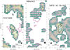 |
Fig. A.1. Grid of the spectra showing the spatial variation of CO(2-1) emission-line profiles of NGC 6860, Mrk 915, and MCG-01-24-012. Each grid spectrum is the sum of all individual spectra inside a region equivalent to the observation beam (gray ellipses). All spectra are normalized for better visualization. The velocity range of the profiles is (-400, 400) km s−1. For reference, the CO flux distribution is shown in the translucent colormap. Overlaid are outer contours from the VLA 3.6 cm radio (in blue) and the smoothed HST [O III] emission (in reddish-purple). We note that the measurements presented on Tables 3 and 4 were calculated from individual spaxels, and not from the integrated spectra presented in these grids. |
Appendix B: Moments and mask
To calculate the moments, we used only pixels that were not masked. These 3D masks were generated reproducing a procedure described in Di Teodoro & Fraternali (2015): first, the original data cubes were smoothed, channel by channel, by convolution with their beam multiplied by a factor of kmult = 2; then, any resulting values below a kcut = 2 σrms cut were masked. For Mrk 915, we used values of kmult = 3 and kmult = 1. Figures 2a, 3a and 4a show that M1 and M2 maps are less extended relative to M0. This happens because we added another constraint: we masked pixels with flux density below 3 σ in the non-convolved data. This was necessary since these M1 and M2 are more affected by pixels with low S/N. The 3D mask was only used to obtain the moments, but a spectrally collapsed 2D version was used in the other analysis as the limit of the CO emission.
Appendix C: Leading spiral arms in Mrk 915?
Figure C.1 displays the maps of the ratio between images in g- and z-bands taken with filters of the Dark Energy Camera. As described in Sect. 4.2, the g / z ratio map was used as a proxy for dust attenuation and to identify the near side of the galaxy disk. More attenuated regions (lower g / z ratio values) are expected to be observed at the near side of the disk. In particular, for Mrk 915, the map presents lower values at the southeast of the nucleus, indicating that the near side of the disk is to the southeast. However, if the stars and CO co-rotate in putative trailing arms, from the CO(2-1) M1 velocity field (Fig. 3a), the near side should be on the west: a contradiction. Is Mrk 915 a rare case of a galaxy with leading arms?
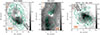 |
Fig. C.1. Maps of the ratio between images obtained at the g- and z-bands (from Dark Energy Camera), used as a proxy for dust attenuation. The CO(2-1) M0 outer contours are overlaid in blueish-green color. The near side of the disk is the southeast and the northwest in NGC 6860, and MCG -01-012-24, respectively. For Mrk 915, the g / z map (middle panel) suggests that the near side of the disk could be in the east, but this would result in Mrk 915 having a rare case of leading arms (see discussion in Sect. C). |
Part of the confusion might originate from the spiral arms and dust lanes being mostly close and along the galaxy’s photometric major axis (instead of the minor axis), making the contrast with the bulge’s light more subtle. Consequently, using dust attenuation to discover the orientation of the disk in Mrk 915 might lead to erroneous conclusions. This strategy also depends on the Mrk 915’s optical continuum having a significant contribution from the bulge’s stellar light, which we could not confirm due to the lack of a bulge-to-disk decomposition in the literature for this object.
If we reverse the orientation – assuming that the near side is to the west – then the arms would be trailing. In this case, the dynamics of the Mrk 915’s spiral arms would follow the expected from most theoretical models (e.g., Evans & Read 1998) and simulations (e.g., Sellwood & Athanassoula 1986), where leading arms are expected to be more unstable, with a posterior decay to a trailing arms motion (Toomre 1981). But we note that long-living leading arms have also been proposed (e.g., Lieb et al. 2022). On the observational side, Iye et al. (2019) found that all objects in a sample of 146 galaxies possess trailing arms, with the authors using the prevalence of dust lanes along the minor axis to identify the near side of the galaxy disk, reproducing the results found by de Vaucouleurs (1958). A rare case of a galaxy with evidence of leading arms is NGC 4622 (Byrd et al. 2008). In that work, the authors suggest that the phenomenon could be a consequence of an encounter with a companion, as reproduced in simulations (e.g., Byrd et al. 1993), which is a scenario that cannot be discarded in Mrk 915 due to the presence of nearby objects (see Fig. 1). Other proposed examples are ESO 297-27 (Grouchy et al. 2008), and IRAS 18293-3134 (Väisänen et al. 2008), both with nearby companions, with the latter one being more similar to Mrk 915 given the absence of outer spirals wound up in the opposite direction from the inner ones.
Since we cannot be sure of the true orientation, we used the observation of stronger dust attenuation to identify the near side of the disk as the default in the figures (near side in the east). Nevertheless, we also consider the opposite orientation in the analysis and discussion of this galaxy.
Appendix D: Disk model fit
We fit the LoS velocity distributions (vc1) using a disk model with circular orbits with velocity (Vc) of the form (Bertola et al. 1991)
 (D.1)
(D.1)
with Vmax being the maximum circular velocity, and p a parameter that governs the shape of the radial velocity profile. For the fit, we also consider that the observed LoS velocity depends on the inclination (i) of the disk, the position angle (PA) of the kinematic major axis, and the systemic velocity of the host galaxy vsys. The kinematic model center was fixed at the ALMA millimeter continuum peak (see Table 1).
Following Bertola et al. (1991), we let p range between 1 (asymptotically flat) and 3/2 (finite total mass). The spatial scale parameter c0 is such that, in r = c0 for p = 1, the circular velocity is Vc(r = c0)∼0.7vmax. Note that the units of the denominator and the “r” in the numerator only cancel out when p = 1. Otherwise, there is an excess of [r]1 − p, where [r] is the unit of distance used during the fit ([r] = ″, in our case). We emphasize that the above velocity function was used to model the velocity field, in order to analyze the velocity residuals, and therefore it should ultimately be considered only an analytical model.
Fig. 7 also shows the best model and the residuals (for both components), while Table 2 lists the best-fit parameter values. The values and uncertainty are the mean and standard deviation, resulting from 100 fits done on the original velocity field – the masked vc1 map (in km s−1) – added by a Gaussian random noise. This noise map was scaled by the cube channel width (in km s−1), which is of the order of the spectral resolution, although larger since we re-binned the data cubes (see Sect. 3). Each fit is done by minimizing the residuals.
Appendix E: Mass outflow and inflow rate
Here, we describe how the outflow and inflow-related quantities were calculated and later displayed in Tables 3 and 4. The cold molecular gas masses (Mmol) were calculated from the velocity-integrated fluxes (SνΔvCO(2 − 1)) using the same method detailed in Paper I. In brief, in each spaxel, SνΔvCO(2 − 1) was derived from the Gaussian profiles fit to the emission lines (Sect. 4.3), and then converted to CO(2-1) luminosities (L′CO(2 − 1), Solomon et al. 1997). The CO(1-0) luminosity was obtained after assuming a ratio of r21 = L′CO(2 − 1)/L′CO(1 − 0) = 0.8 – 1.2, typical of nearby galaxies (Braine & Combes 1992), Finally, Mmol are estimated using a conversion factor of αCO = MH2/L′CO(1 − 0) = 0.8 – 4.3 M⊙ [K km s−1 pc−2]−1, covering a wide range of physical conditions for the clouds, with the αCO limits corresponding to average values obtained for in ultra luminous infrared galaxies and in the Milk Way (Bolatto et al. 2013b).
E.1. Mass inflow rate
Based on Storchi-Bergmann et al. (2007), Riffel et al. (2008), we calculated the mass inflow rate by assuming a constant flow over a cylindrical geometry  , where Vin is the deprojected inflow velocity, A is the cross-section area of an elliptic cylinder, and ρmol is the volumetric mass density of the cold molecular gas inside the cylinder. If we calculate the density inside the cylinder from ρmol = Mmol, in/(h A), the mass inflow rate becomes simply:
 (E.1)
(E.1)
where is h is the projected length of the cylinder, Mmol, in is the molecular mass inside it and Vin is the de-projected inflow absolute velocity.
We can also estimate the average volumetric mass density in the inflows using ρmol = Mmol, in/(hπra rd), where ra is the deprojected major radii of cylinders faces and 2 rd is the disk height, assumed to be 2 rd ∼ 30 pc (Hicks et al. 2009). In addition, the volumetric number density of molecular clouds can be calculated from nmol = ρmol/(1.36 ⋅ 2 mp) ∼ 4 – 30 cm−3, where mp is the proton mass, and 1.36 factor accounts for 36 % contribution from Helium (Saintonge & Catinella 2022).
NGC 6860. Using Eq. E.1 and assuming a constant inflow rate inside the cylindrical geometry (sketch in left panel of Fig. E.1) we found cold molecular mass inflow rates of:  ∼ 0.34 – 2.7 M⊙ yr−1, from the north of the nucleus, at the far side of the disk; and
  ∼ 0.46 – 3.7 M⊙ yr−1, from the south. And integrating from both directions: Ṁmol,in ∼ 0.8 – 6 M⊙ yr−1 (see Table 3), with the large uncertainty being dominated by the uncertainty in the αCO value. These values are obtained assuming an inclination of i = 57.7°, for an inflow coplanar with the disk. In the above calculations, we used as the de-projected inflow velocities values:
  ∼ −90 km s−1 and
  ∼ 90 km s−1 (the superscript number matches the numeration in Fig. E.1). These values correspond to the average of the LoS residuals – relative to the disk model – of the c1-component inside the dashed ellipses of Fig. E.1. After integrating the flux inside these ellipses, we obtained molecular masses of
  ∼ (0.34 – 2.6) × 107 M⊙ and
  ∼ (0.8 – 6.5) × 107 M⊙ in each region, resulting in a total of Mmol, in ∼ (1 – 9) × 107 M⊙. The deprojected cylinder lengths used in the calculation are h(1) ∼ 1.6″∼ 900 pc and h(2) ∼ 2.8″∼ 1.6 kpc.
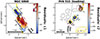 |
Fig. E.1. Geometry of the molecular inflow along the bar (dashed yellow line) in NGC 6860 and along one of the spiral arms in Mrk 915 (assuming that the arms are leading). The yellow elliptic cylinders have heights, h, and areas, A = πrard, where rd is half the height of the disk and ra is the major radius of the face (see inset in the right panel). The superscript numbers identify the regions used in calculations in Sect. E.1. The cylinders are drawn over the LoS residuals of the disk model (as Fig. 7). These residuals associated with components used in the Ṁmol,in calculations: c1 for NGC 6860 and c2 for Mrk 915. The reddish-purple and blue dashed ellipses delimit the regions used to obtain the velocities and masses of the inflows coming from the north and the south in NGC 6860. For Mrk 915, they mark the region of the farthest and the nearest inflowing clumps. |
Using  ∼ 0.29″ ∼ 160 pc and
  ∼ 0.42″ ∼ 240 pc as values for deprojected major radii of cylinders’ faces (see Fig.E.1), we obtained a volumetric mass density in the inflows of ρmol = ∼ 0.2 – 2 M⊙ pc−3. Here, ρmol is the average of the values obtained for the north and the south inflows, which are approximately equal. This corresponds to a volumetric number density of molecular clouds of nmol ∼ 3 – 30 cm−3.
Mrk 915 (leading arms scenario). Applying the Eq. E.1 individually for each inflowing CO clump of Mrk 915 (see sketch in Fig. E.1), we obtained mass inflow rates of: Ṁmol,in ∼  ∼
∼  ∼ 0.09 – 0.8 M⊙ yr−1. Since the inflows come from the same direction, we average the mass inflow rates from both clumps, which have essentially the same value. The inflow de-projected velocities of each clump are
  ∼ −100 km s−1 and
  ∼ −160 km s−1, while the molecular masses are
  ∼ (0.35 – 3.0) × 106 M⊙ and
  ∼ (0.56 – 4.8) × 106 M⊙. Here, we assumed an inflow inclination of i = 66.5° (coplanar with the disk).
For each clump, we considered the values of c2-component inside the blue (farthest clump) and reddish-purple (nearest) dashed ellipses shown in Fig. E.1. We assumed the same geometry for both cylinders: h(3) = h(4) =  =
=  ∼ 0.5″∼ 600 pc, using an inclination of i = 66.5°. The average volumetric mass and number densities are ρmol ∼ 0.03 – 0.2 M⊙ pc−3 and nmol ∼ 0.4 – 3 cm−3, respectively, with the densities being ∼ 2 times higher in the farthest clump.
E.2. Mass outflow rate
By assuming that the mass outflow rate is constant over time, we could calculate it using (Lutz et al. 2020):
 (E.2)
(E.2)
In the equation, Mmol, out is the total outflowing gas mass, and Vout and Rout are the de-projected maximum outflow velocity and extent, respectively.
NGC 6860. The total molecular mass of the outflowing clouds in NGC 6860 is Mmol, out ∼ 0.6 – 5 × 10⁶ M⊙, as obtained from the flux of the component c2 of SνΔvCO(2 − 1),out = 340 ± 6 Jy km s−1, integrated inside a 0.6″ radius (see Table 4). This corresponds to ∼ 0.7 % of the total molecular mass in the galaxy observed within a radius of ∼ 13″. Assuming that the outflow is almost coplanar to the galaxy disk (inclination i = 57.7°), the de-projected maximum velocity and outflow extent are Vout ∼ 140 km s−1 and Rout ∼ 560 pc, respectively. Using this values in Eq. (E.2), we obtained a mass outflow rate of Ṁmol,out ∼ 0.1–1 M⊙ yr−1.
Mrk 915 (trailing arms scenario). Considering only the CO emission from the component c2 with negative LoS residuals (nearest two clumps, see Fig 7), the mass of the outflowing clouds is Mmol, out ∼ 0.8 – 7 × 10⁶ M⊙ (from SνΔvCO(2 − 1),out = 184±4 Jy km s−1), which is ∼ 4 % of the total cold molecular mass. Therefore, using Eq. E.2, the cold molecular gas mass outflow rate is Ṁmol,out ∼ 0.09 – 0.7 M⊙ yr−1, for Vout ∼ 300 km s−1 and Rout ∼ 2.8 kpc (de-projected values), where we assumed an outflow inclination coplanar with the disk (i = 66.5°).
MCG -01-24-012 (CND scenario). The total CO(2-1) flux in the CND double-peak region of MCG -01-24-012 is SνΔvCO(2 − 1),out ∼ 9.22±0.01 Jy km s−1 including the flux of both components. This corresponds to a molecular gas mass of ∼ 3 – 20 × 107 M⊙, representing ∼ 30 % of the total observed cold molecular mass. For a molecular outflow close to plane of the CND (inclination i = 74° in our preferred model), the corresponding mass outflow rate is Ṁmol,out ∼ 0.4 – 3 M⊙ yr−1. To obtain Ṁmol,in, we used Eq. E.2, with a de-projected outflow velocity and extent of Vout ∼ 40 km s−1 and Rout ∼ 3 kpc (∼ 2″), respectively. The Vout corresponds to the mean absolute difference between the velocities of the components relative to our preferred disk model for the CND.
Appendix F: Additional figures
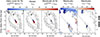 |
Fig. F.1. Similar to Fig. 7, but for the fit done using only the CO data (from component c1) along the stellar bar in NGC 6860. |
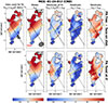 |
Fig. F.2. Similar to Fig. 7 but for the fit done in the region with double-peak profiles of MCG -01-24-012 to model the CND rotation. In the first row, the PA parameter was set free during the fit, which resulted in a face-on disk, while in the second row, we fixed PA at 0°, resulting in a more inclined disk. The data used to fit the disk model corresponds to the average between the LoS velocities of the components c1 and c2 in the double-peak region (black contours). The first three columns show the LoS velocity data, the best-fit rotation model, and the residuals of the fit data. The last two columns correspond to the residuals of each component. The dotted and dashed black lines are the kinematic major axes of the CND models and the global model (Fig. 7). The orange dashed line indicates the position of the stellar bar. |
All Tables
All Figures
|
Fig. 1. Color-composite images from DESI Legacy Survey Sky Viewer showing the local environment of NGC 6860 (left), Mrk 915 (middle) and MCG -01-24-012 (right), with squares marking the FoV of Figs. 2a, 3a and 4a. The spectroscopic redshifts of the brighter sources correspond to the preferred values from the NASA/IPAC Extragalactic Database. North is up and east is left in this and the remaining figures in the paper. |
| In the text | |
|
Fig. 2. Maps of NGC 6860. (a) Spatial distributions of the CO(2-1) moments maps of the observed spectral profile, with M0 corresponding to the integrated flux, M1 tracing the mean radial velocity, and M2 representing the velocity dispersion of the CO profile. (b) Maps of the parameters of the two Gaussian components fit the CO(2-1) profiles: c1 (top row) and c2 (bottom row). The columns correspond to distributions of the flux (left), the LoS velocity (middle), and the velocity dispersion (right). In the bottom row, contours outline the full CO(2-1) extent (in gray) and the double-peak region (in black). In the bottom-left map, we added dashed lines representing the spiral arms (orange), the stellar bar (yellow), and the ring (sky-blue), as identified in Paper I. The letters A – E in the lower-left panel show the locations of the spaxels used as examples of fits in Fig. 5. For this and all other maps in the paper: North is up and east is left. The coordinates are relative to ALMA millimeter continuum peak (black cross marks, see Table 1), assumed to be to the galactic nucleus. The gray ellipses correspond to the ALMA beam size of the observation. The inclined black dotted line is the major axis of the global kinematic model. |
| In the text | |
 |
Fig. 3. Same as Fig. 2, but for Mrk 915. |
| In the text | |
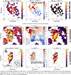 |
Fig. 4. Same as Fig. 2, but for MCG -01-24-012. |
| In the text | |
|
Fig. 5. Example of the model multiple Gaussian models fit to the CO(2-1) profiles of individual spaxels (0.076–0.16″ sizes), one row per object. The first four columns (A to D) show examples where two Gaussian components were preferred over a single component, as in the last column (E). The spatial positions (relative to the nucleus) of each spaxel are shown at the top of each panel and are marked in Figs. 2a, 3a and 4a (blue letters in the lower left panels). The lines represent: original data (bluish-green); one Gaussian component models (in blue); two Gaussian models (in orange), along with their individual components (in black dashed). The residuals of both models are shifted downward in the plots. The y-axes are in units of S/N. The horizontal dotted line corresponds to S/N = 3 and is highlighted since this was the threshold used to discard components. |
| In the text | |
|
Fig. 6. Position-velocity maps for the CO(2-1) of each object for 1″-width pseudo-slits along three different positions: kinematics major and minor axis (first two columns) and along the double-peak (dp) region (last column). We added the individual LoS velocities obtained for the Gaussian components c1 (blue circles) and c2 (orange circles) fit to the spectral profiles. The bluish-green lines correspond to the global rotating disk model fit to the single-peak (sp) region (first three rows in Table 2). For NGC 6860, three models are shown, which were fit using data from the ring (bluish-green line), from the bar (dot-dashed black line), and combining data from both ring and bar (long dashed black line). For MCG -01-24-012, we also added curves from two models fit in the double-peak region, one letting the PA free (short dashed black line) and the other with PA = 0° (dotted black line). |
| In the text | |
|
Fig. 7. Comparison between the CO(2-1) data obtained from the Gaussian decomposition of the profiles and the rotating 2D disk model (first three rows in Table 2). The first three columns show the distributions of the LoS velocity of the c1-component (vc1), the best-fit rotation model, and the residuals from the fit. The model was fit to the single-peak region of the vc1 data (masked regions not shown). An additional mask was used for the inner regions of NGC 6860, restricting the fit to regions dominated by rotation in the disk. The last two columns are a zoom-in showing residuals of each component (c1 and c2), with the models extended to the double-peak region. The black contours encircle the masked regions with double-peak CO profiles, while the gray contours show the full data extent. The dashed lines identify stellar structures: bars (yellow), spirals (orange), and rings (sky-blue). |
| In the text | |
|
Fig. 8. Schematic models for our proposed scenarios of NGC 6860, Mrk 915, and MCG -01-24-012. The second row corresponds to a zoom-in in the central regions. Due to the ambiguous orientation of the Mrk 915 disk (see Appendix C), we added both scenarios of spiral arms motion: trailing and leading. The contours represent the flux distribution of: cold molecular gas from CO(2-1) M0 (bluish-green), ionized gas from HST [O III] (reddish-purple), VLA 3.6 cm radio (blue), and the CO double-peak region (black). For a better view, we plotted only a few contour levels and manually cleaned isolated ones. Stellar structures are drawn in dashed lines: spiral arms (in orange), stellar rings (sky-blue), and bars (yellow). The gray “3D” planes correspond to the plane of the global rotating disk model. We also added “3D” bipolar ionized cones to represent possible orientations of these structures. The senses of rotation of the spirals are shown in orange dashed arrows, assuming that they “follow” rotation of the CO. The solid arrows represent the direction of motion of: components c1 (blueish-green) and c2 (black) of the CO(2-1), ionized gas (reddish-purple) and radio-jets (blue), with curved lines representing rotation. We added question marks to represent that we can only confirm the kinematics of the [O III] using resolved integral-field observations, and the same for the possible radio jets that need deeper and higher spatial resolution observations. In the double-peak regions, we added one arrow for each component. In particular, for MCG -01-24-012, we tried to represent that both components are dominated by rotation, with each one having an extra positive/negative radial velocity “kick” due to the CO being disturbed equatorially by the ionized outflow. |
| In the text | |
|
Fig. 9. Position-velocity map of NGC 6860, similar to Fig. 6, but for a position angle along the bar and with a slit width of 1.5″, matching the observations from Lipari et al. (1993). We added their observed LoS velocities from the stellar absorption lines of Ca II K (triangles) and Na I D (crosses) in reddish-purple color and the ionized gas emission lines of [O III] (star symbols) and H α (‘x’ markers) in sky blue. |
| In the text | |
|
Fig. 10. Distribution of the LOS velocity versus the distance along the global kinematic major axis (PA = 32.0°, inside a 0.27″ slit width) of MCG -01-24-012. Values in the single-peak region are shown as blueish-green circles (component c1), while values in the double-peak region are shown as blue (for c1) and orange circles (for c2). The black circles correspond to the average between the LoS velocities of both components (vrot, CND). In the top row, along with the LoS velocity values of each component, we show lines representing models fit to the data. The global disk model, obtained in the single-peak region (see Fig. 7), is shown as a blueish-green line, with the residual shown in the second row. We show two models fit in the CND region (see maps in Fig. F.2, and schematic models in Fig. 11): one with the a free PA parameter (black dashed line, with the residuals in the third row); and another with PA = 0° fixed (black dotted line, with the residuals in the forth row).
|
||
| In the text | |||
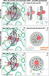 |
Fig. 11. Possible geometries for the CND in MCG -01-24-012. The legend from Fig. 8 also applies here. The left and right columns show the observation and lateral views, respectively. On the right, we added arrows to represent the velocity vectors of the components c1 (blue) and c2 (orange), decomposed in the rotating (bluish-green) and outflowing (black) parts, with diagrams. As in Fig. 8, the orientations of the ionized cones were chosen to try to reproduce the [O III] emission (reddish-purple contours). In the first row, the face-on CND is the result of fitting a rotating disk model with free PA. In this scenario, the CO double peaks would result from expanding clouds perpendicular to the disk. In the last row, we show another way of reproducing the double peaks by assuming an edge-on disk geometry, with the outflow occurring radially along the disk. Our preferred scenario lies between these two geometries, as shown in the middle row. This model is the result of fixing PA at 0° to reproduce the CO flux distribution, which yields an inclination of 74°. |
| In the text | |
|
Fig. A.1. Grid of the spectra showing the spatial variation of CO(2-1) emission-line profiles of NGC 6860, Mrk 915, and MCG-01-24-012. Each grid spectrum is the sum of all individual spectra inside a region equivalent to the observation beam (gray ellipses). All spectra are normalized for better visualization. The velocity range of the profiles is (-400, 400) km s−1. For reference, the CO flux distribution is shown in the translucent colormap. Overlaid are outer contours from the VLA 3.6 cm radio (in blue) and the smoothed HST [O III] emission (in reddish-purple). We note that the measurements presented on Tables 3 and 4 were calculated from individual spaxels, and not from the integrated spectra presented in these grids. |
| In the text | |
|
Fig. C.1. Maps of the ratio between images obtained at the g- and z-bands (from Dark Energy Camera), used as a proxy for dust attenuation. The CO(2-1) M0 outer contours are overlaid in blueish-green color. The near side of the disk is the southeast and the northwest in NGC 6860, and MCG -01-012-24, respectively. For Mrk 915, the g / z map (middle panel) suggests that the near side of the disk could be in the east, but this would result in Mrk 915 having a rare case of leading arms (see discussion in Sect. C). |
| In the text | |
|
Fig. E.1. Geometry of the molecular inflow along the bar (dashed yellow line) in NGC 6860 and along one of the spiral arms in Mrk 915 (assuming that the arms are leading). The yellow elliptic cylinders have heights, h, and areas, A = πrard, where rd is half the height of the disk and ra is the major radius of the face (see inset in the right panel). The superscript numbers identify the regions used in calculations in Sect. E.1. The cylinders are drawn over the LoS residuals of the disk model (as Fig. 7). These residuals associated with components used in the Ṁmol,in calculations: c1 for NGC 6860 and c2 for Mrk 915. The reddish-purple and blue dashed ellipses delimit the regions used to obtain the velocities and masses of the inflows coming from the north and the south in NGC 6860. For Mrk 915, they mark the region of the farthest and the nearest inflowing clumps. |
| In the text | |
|
Fig. F.1. Similar to Fig. 7, but for the fit done using only the CO data (from component c1) along the stellar bar in NGC 6860. |
| In the text | |
|
Fig. F.2. Similar to Fig. 7 but for the fit done in the region with double-peak profiles of MCG -01-24-012 to model the CND rotation. In the first row, the PA parameter was set free during the fit, which resulted in a face-on disk, while in the second row, we fixed PA at 0°, resulting in a more inclined disk. The data used to fit the disk model corresponds to the average between the LoS velocities of the components c1 and c2 in the double-peak region (black contours). The first three columns show the LoS velocity data, the best-fit rotation model, and the residuals of the fit data. The last two columns correspond to the residuals of each component. The dotted and dashed black lines are the kinematic major axes of the CND models and the global model (Fig. 7). The orange dashed line indicates the position of the stellar bar. |
| In the text | |
Current usage metrics show cumulative count of Article Views (full-text article views including HTML views, PDF and ePub downloads, according to the available data) and Abstracts Views on Vision4Press platform.
Data correspond to usage on the plateform after 2015. The current usage metrics is available 48-96 hours after online publication and is updated daily on week days.
Initial download of the metrics may take a while.