| Issue |
A&A
Volume 705, January 2026
|
|
|---|---|---|
| Article Number | A64 | |
| Number of page(s) | 20 | |
| Section | Stellar structure and evolution | |
| DOI | https://doi.org/10.1051/0004-6361/202556074 | |
| Published online | 06 January 2026 | |
Filamentary accretion flows in high-mass star-forming clouds
1
Max-Planck Institut für Astronomie, Königstuhl 17, D-69117 Heidelberg, Germany
2
Fakultät für Physik und Astronomie, Universität Heidelberg, Im Neuenheimer Feld 226, D-69120 Heidelberg, Germany
3
Zentrum für Astronomie der Universität Heidelberg, Albert-Ueberle-Str. 2, D-69120 Heidelberg, Germany
4
Department of Astronomy, Xiamen University (Haiyun Campus), Zengcuo’an West Road, Xiamen, 361995
China
5
UK Astronomy Technology Centre, Royal Observatory, Edinburgh, Blackford Hill, Edinburgh, EH9 3HJ
UK
6
INAF – Osservatorio Astrofisico di Arcetri, Largo Enrico Fermi 5, I-50125 Firenze, Italy
7
INAF – Osservatorio Astronomico di Cagliari, Via della Scienza 5, I-09047 Selargius (CA), Italy
8
Centre for Astrophysics and Planetary Science, University of Kent, Canterbury, CT2 7NH
UK
9
Instituto de Radioastronomía y Astrofísica, Universidad Nacional Autónoma de México, Antigua Carretera a Pátzcuaro 8701, Ex-Hda. San José de la Huerta, 58089 Morelia, Michoacán, México
10
Department of Physics and Astronomy, McMaster University, Hamilton, ON, Canada
★ Corresponding author: This email address is being protected from spambots. You need JavaScript enabled to view it.
Received:
24
June
2025
Accepted:
28
October
2025
Abstract
Context. Filamentary accretion flows as gas-funneling mechanisms are a key aspect in high-mass star formation research. The kinematic properties along these structures are of particular interest.
Aims. This paper focuses on the question of whether gas is transported to dense clumps inside high-mass star-forming regions through filamentary structures, from scales of several parsecs down to the subparsec scale.
Methods. We quantified the gas flows from a scale of up to several parsecs down to the subparsec scale along filamentary structures. For this work the accretion flow mechanisms based on gas kinematic data in the three high-mass star-forming regions G75.78, IRAS21078+5211, and NGC7538 were studied with data obtained from the IRAM 30 m telescope. The analysis was carried out using the surface density derived from 1.2 mm continuum emission and velocity differences estimated from HCO+ (1 − 0) and H13CO+ (1 − 0) molecular line data.
Results. The mass flow behavior of the gas in the vicinity of high-mass star-forming clumps shows characteristic dynamical patterns, for example an increased mass flow rate toward the clumps. We assume that the velocity differences originate from filamentary-gas infall onto the high-mass star-forming clumps; however, the inclination of the filament structures along the line of sight is unknown. Nevertheless, using the velocity differences and mass surface densities, we can estimate the mean flow rates along the filamentary structures with respect to the line of sight and toward the clumps. We quantified the flow rates toward the clumps in a range from about 10−3 M⊙ yr−1 to 10−5 M⊙ yr−1, inferred from clump-centered polar plots. Slight variations in the flow rates along the filamentary structures may be caused by overdensities and velocity gradients along the filaments.
Conclusions. While the initial studies presented here already reveal interesting results such as an increasing mass flow rate toward clumps, the properties of filamentary gas flows from large to small spatial scales, as well as potential variations over the evolutionary sequence, are subject to future studies.
Key words: stars: formation
© The Authors 2026
 Open Access article, published by EDP Sciences, under the terms of the Creative Commons Attribution License (https://creativecommons.org/licenses/by/4.0), which permits unrestricted use, distribution, and reproduction in any medium, provided the original work is properly cited.
This article is published in open access under the Subscribe to Open model.
Open Access funding provided by Max Planck Society.
1. Introduction
Understanding filamentary accretion flows as a central mechanism in high-mass star formation is still an open field of research; many aspects are still unkown (e.g., Hacar et al. 2023; Pineda et al. 2023). Theory provides us with models of cloud-collapse, fragmentation and other processes that lead to filamentary accretion flows in giant molecular clouds (GMCs) and molecular clouds (MCs) (e.g., Smith et al. 2012, 2014, 2016; Vázquez-Semadeni et al. 2019; Padoan et al. 2020; Zhao et al. 2024). The difference between GMCs and MCs is their mass: GMCs are larger and much more massive, exceeding 105 M⊙. In this study we focus on parsec-scale accretion flows from the cloud environment onto the dense high-mass clumps prone to massive cluster formation.
Source parameters from the CORE sample (as listed in Beuther et al. 2018).
The three star-forming regions studied in this paper are G75.78 with the main clump G75.78+0.34 (hereafter G75), IRAS21078+5211 (hereafter IRAS21078), and NGC7538, consisting of NGC7538 IRS1, NGC7538 S, and NGC7538 IRS9. The sources are part of the CORE program (Beuther et al. 2018; Beuther 2020; Gieser et al. 2021; Ahmadi et al. 2023; Beuther et al. 2024). We summarize their main parameters in Table 1. According to their estimated masses and equivalent radii of about 1 pc, we refer to them as clumps throughout this work. They have been subject to studies in the past; young stellar objects (YSOs) and HII1.2ex regions have been observed in all regions (see e.g., Riffel & Lüdke 2014; Moscadelli et al. 2021; Beuther et al. 2022). While the initial aim was to include all CORE regions in this survey, we only obtained data for three of them due to weather conditions during the observing window. All regions would have represented a broader range of mass regimes; this is why IRAS21078 is included in this work despite its lower mass compared to the other two sources.
Filament structures and hubs were studied in other star-forming regions in the past, and velocity gradients along filaments were identified (e.g., Peretto et al. 2013, 2014; Kim et al. 2022; Ma et al. 2023). However, whether the observed velocity differences traced by molecules are signatures of flows inside filament structures is still not entirely clear. In this work we investigate such structures in all three regions in detail and apply a simple mass flow estimation model. The mass flow approach quantifying accretion flows in high-mass star-forming regions has already been outlined and used in previous studies (e.g., Beuther 2020; Wells et al. 2024). On the theoretical side, processes from large to small scales have been modeled and categorized, for example, into inertial infall and subsequent inflow, followed by accretion onto prestellar clumps (e.g., Smith et al. 2012, 2014, 2016; Padoan et al. 2020; Zhao et al. 2024). On the other hand, the formation of filamentary structures inside GMCs and MCs is assumed to be a direct consequence of enhanced anisotropy during cloud collapse and fragmentation, after which the filaments act as channels where gas is funneled onto the prestellar clumps (e.g., Vázquez-Semadeni et al. 2019; Padoan et al. 2020). Most simulations also show that the formation of filaments is a consequence of crossing shocks (Vázquez-Semadeni et al. 2003; Mac Low & Klessen 2004; Krumholz et al. 2005; Hennebelle & Chabrier 2011; Padoan & Nordlund 2011; Federrath & Klessen 2012; Pudritz & Kevlahan 2013). The analysis of the high-mass star-forming MCs in this work generally takes into account scales of several parsecs down to the subparsec scale.
The structure of the paper is as follows. We start by introducing the data in Sect. 2, and also give a brief overview of the reduction process and archival data. We then focus on the mass flow analysis in Sect. 3. We conclude this analysis with a summary and outlook in Section 4.
2. Observation
We present the NIKA2 1.2 mm dust continuum emission maps for all three sources in Fig. 1. The first moment maps (intensity weighted peak velocities) from HCO+ and H13CO+ for the kinematic analysis are shown in Figs. 2 and 3, respectively. We summarize the RMS values for the molecular data in Table 4. Data reduction and analysis have been conducted using the GILDAS1 framework with the subprograms CLASS and GREG.
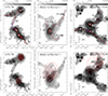 |
Fig. 1. Top row: NIKA2 1.2 mm dust continuum maps (see Beuther et al. 2024) of the star-forming regions showing the clump and filament designations. The red and magenta markers indicate the data points used for the flow rate estimation in Section 3.2. The triangular magenta markers indicate a separate section along a structure. Black contours outline the 1.2 mm continuum, ranging from 3σ to 39σ in steps of 3σ (the RMS values are presented in Table 5). The red contours in the upper panels mark the peak positions of the continuum emission from 20% to 100% in steps of 20%. The designations used in the following refer to clumps and filament structures, filaments are labeled F; CF in G75 is the central filament; CC in IRAS21078 is the central clump. The clumps in NGC7538 are the known objects IRS9, IRS1 and S (e.g., Beuther 2020). G75 S1 is the object G75.78+0.34. We present the clump designations together with their coordinates in Table 3. Bottom row: Same dust-maps, but with red contour lines outlining the HII1.2ex regions at 1.4 GHz (21 cm) (Condon et al. 1998); the contours range from 10% to 100% of the peak emission in steps of 10% (see Table 5 for reference). The positions of the two main exciting sources of the HII1.2ex region in NGC7538, NGC7538 IRS5 and NGC7538 IRS6, are marked in the lower right panel (Puga et al. 2010). |
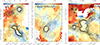 |
Fig. 2. First moment (intensity-weighted peak velocity) maps for the HCO+ (1 − 0) line. The beam size is 27″ (lower left corner). The sources are labeled in each panel. The scale bar indicates the length of 1 parsec in each panel. The contour lines show the 1.2 mm dust continuum ranging from 3σ to 39σ in 3σ steps. |
Overview of the molecular properties for the two molecules presented in this paper.
Clump designations and their coordinates.
Overview of σrms values of the molecular transitions at a spectral resolution of 0.9 km s−1.
2.1. IRAM 30 m EMIR observation
We used three different sets of data for this analysis: The IRAM 30 m spectral line data were observed in 2021 (project ID 121-20) as part of the CORE program (Beuther et al. 2018) with a beam size of 27″ in the 3 mm band. The raw data were calibrated to the main-beam temperature Tmb with a beam efficiency of 76%. The spectral resolution is 0.9 km s−1. We identified the HCO+ line at a frequency of 89.189 GHz in the upper sideband as the J = 1-0 transition, with a Eu/k value of 4.3 K and the H13CO+ emission as J = 1-0 at 86.754 GHz with Eu/k = 4.2 K. We list the molecular properties in Table 2. The moment maps were produced with a lower intensity threshold of 4σ (cf. Table 4). Because we noted some absorption features in the optically thick HCO+ compared to the optically thin H13CO+ (Fig. 5), we also included the latter molecular data in the analysis (Fig. 3).
Peak- and σrms values of the 1.2 mm dust continuum and the 1.4 GHz (21 cm) data (HII1.2ex regions).
We derived dust temperature maps by applying the iterative spectral energy distribution (SED) fitting procedure outlined by Lin et al. (2016), using both Herschel data and the NIKA2 1.2 mm maps. Figure 4 are the temperature maps, Prior to SED fitting, the NIKA2 1.2 mm map was corrected for missing large-scale flux and free–free emission. Large-scale structures were recovered by combining the NIKA2 map with Herschel data in the Fourier domain using the J-comb algorithm (Jiao et al. 2022). The combined map was then convolved to 27″ to match the angular resolution of the free–free emission map, which was derived based on H41α observations (for a detailed explanation, see Gieser et al. 2023, Section 4.2). Finally, the free–free corrected NIKA2 1.2 mm map was obtained by subtracting the free–free contribution from the combined map. Single-component modified blackbody fits were performed pixel by pixel after convolving all maps to a common beam size and regridding to the same pixel scale. In the iterative fitting process (Lin et al. 2016), the final dust temperature maps were obtained at 27″ resolution.
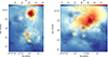 |
Fig. 4. Dust temperature maps of G75 (left panel) and NGC7538 (right panel). Both maps were created using Herschel data (Molinari et al. 2010) and free–free corrected dust continuum emission from the NIKA2 dataset. In the bottom left corner the 27″ beam of the final data product is shown. The black contours outline the free–free corrected 1.2 mm continuum emission at 27″ resolution in logarithmic scale from 5σ to peak value. |
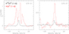 |
Fig. 5. Spectra toward G75 showing molecular emission of HCO+ (1 − 0) (red) and H13CO+ (1 − 0) (black). The left panel shows the emission at the clump position S1 in G75. The right panel shows the spectra for a position along the CF filament in G75 (see upper left panel of Fig. 1). |
2.2. Archival continuum data
We used 1.4 GHz Very Large Array (VLA) data and temperature data from the Herschel infrared Galactic Plane Survey (Hi-GAL; Molinari et al. 2016; Marsh et al. 2017) and the IRAM 30 m NIKA2 1.2 mm dust continuum data (see e.g., Beuther et al. 2024, Sect. 2.1). The underlying dust continuum maps that we used to identify filament-like structures originated from NIKA2 1.2 mm continuum data from the CORE sample, observed with the IRAM 30 m telescope (Beuther et al. 2024) with a beam size of 12″.
Radio continuum data used to probe the HII1.2ex regions were taken from the NRAO VLA Sky Survey (NVSS) 1.4 GHz VLA survey (see e.g., Condon et al. 1998), the peak and σrms values of both the dust continuum data and the HII1.2ex data are presented in Table 5.
3. Results
In Fig. 2 we show the intensity-weighted peak velocities (first moment) for HCO+ (1 − 0) in the three sources, while we present the same for H13CO+ (1 − 0) in Fig. 3. The lower threshold when creating the maps was set to 3σ. We note the interesting patterns: HCO+ (1 − 0) and H13CO+ (1 − 0) display strong velocity differences of up to a few km s−1 in the vicinity of N1 and prominently between S1 and S2 in G75. We also note the gradients next to the central filament (CF) of G75 and north of G75 S1. Inside IRAS21078, velocity differences of about 1 km s−1 cover the extent of the cloud, with a sharp cutoff close to the eastern–southeastern edge (except for H13CO+ (1 − 0), which is spatially confined to the denser regions of the source). In NGC7538, the velocity differences of ∼1 km s−1 can be seen around IRS1 and S (cf. Fig. 1). Only gravitational infall could have produced these velocity differences. Rotating clumps appears an unlikely candidate since the rotation of clouds on parsec scales has not convincingly been observed. The HII1.2ex regions may impact the velocity structure, which can be seen in the bar-like structure in the northwest of NGC7538 (Fig. 2). In G75, the southern HII1.2ex region is located exactly in the middle of clumps S1 and S2 (Fig. 1), and can even increase the gas flow toward the clump. Similar scenarios could happen in IRAS 21078. Hence, while the HII1.2ex regions may have some influence, in the framework of this analysis, we assume that the velocity gradients are dominated by gas flows toward the clumps.
We also note the lack of HCO+ data in the northern part of NGC7538, but HCO+ (1 − 0) emission toward the peak of the HII1.2ex region (cf. Figs. 1, 2 and 3). The HII1.2ex region is excited by the two sources IRS5 and IRS6 with spectral types of O9 and O3 respectively (Puga et al. 2010), and has already photo-dissociated the molecular gas to a large extent (the other two sources have HII1.2ex regions as well, but no lack of molecular emission from the HCO+ (1 − 0) line). The strong and sharp velocity differences of up to about 4 km s−1 along the northwestern filamentary structure in NGC7538 are therefore likely expected to stem from feedback from the HII1.2ex region, and not from gas infall. This assertion is important for the later interpretation of mass flow behavior inside this source.
As shown in Figs. 5, C.5 and C.6, the main isotopolog can be optically thick toward the main emission peaks and may hence show spectra with multiple peaks, whereas the rarer H13CO+ spectra always have Gaussian profiles, which is typical of optically thin lines. We did not estimate absolute optical depths because that was not needed for our analysis. Since we were interested in the peak velocities, we used the H13CO+ first moment maps to study the velocity field. Where H13CO+ is not detected, the optical depth of HCO+ is probably low because it shows single Gaussian profiles. Therefore, at these positions the HCO+ 1st moment maps can represent the velocity structure well.
3.1. Methods: Flow rate estimates
The estimation of the mass flow rate follows the approach used in Beuther 2020 and discussed in more detail in Wells et al. 2024. The filamentary structures are identified in the dust continuum emission and inclination i relative to the observer is considered within the uncertainties discussed below. We can estimate a mass flow rate as
 (1)
(1)
where Σr is the beam-averaged mass surface density along the filamentary structures, Δvr is the velocity difference between a point and the center of measurement (a high-mass star-forming clump) and Δrr a projected distance along the structures and points of measurement. The mass flow rate estimate is a function of i, where tan(i) has to be non-vanishing; the subscript r indicates the real values for the inclined filament structure (for a detailed derivation, see Wells et al. 2024). The surface density can be estimated from the 1.2 mm dust continuum assuming optically thin emission as (Hildebrand 1983; Schuller et al. 2009)
 (2)
(2)
where Fν is the flux density, R the gas-to-dust ratio (150, Draine 2011), Bν the Planck function at the dust temperature TD, κν the dust absorption coefficient (which was set to 0.9 cm2 g−1, as given in Table 1 Col. 5 in Ossenkopf & Henning 1994), μ the mean molecular weight of the interstellar medium (assumed to equal 2.8), mH the mass of the hydrogen atom, and Ω the solid angle. We measured the flux density Fν from the 1.2 mm dust continuum at 250 GHz and considered the dust temperature obtained for G75 and NGC7538 from the Hi-GAL Galactic Plane Survey (Molinari et al. 2016) as mentioned in Sect. 2. As for IRAS21078, the temperature values were set constant to the characteristic value of 20 K, which has to be considered within the error margins. We checked the impact of the constant temperature with a comparison for G75 and NGC7538, where we averaged over the mass flow rates for each section of measurement and took the ratio of the variable temperature data to the constant temperature data. We estimated an average increase in the mass flow rate for the fixed values of about 75%. We note that the difference in temperature close to peak emission near the clumps is higher, and therefore affects the overall mass flow rate to a larger degree. The systematic errors for the measured quantities in Eqs. (1) and (2) were estimated. We assume a velocity uncertainty of 0.5 km s−1, slightly larger than half the velocity resolution. From the SED fitting, each data point was weighted by its measured noise, yielding an average dust temperature uncertainty of 1 K. We also estimated 5% uncertainty for the flux density (typical calibration uncertainty; see Perotto et al. 2020). Regarding the uncertainties of the projected distances to the center, since these are always relative distances within the maps, we assumed an uncertainty of 1 pixel or 5″. All errors were estimated by applying Gaussian error propagation to Eqs. (1) and (2).
3.2. Flows along filaments
For this part of the analysis we conducted the flux density and velocity difference measurements along filamentary structures identified in the dust continuum maps. We plotted the mass flow rate as a function of the distance along the structure (see Figs. 6, 7, 8). The mass flow rate was estimated with the separation Δr as the half beam size of 13.5″ from the kinematic data and the surface density calculated from the flux value taken at one marker position, whereas the velocity difference was always taken relative to the center of the starting point (a clump; see also Section 3.1). All velocity values were taken preferably from H13CO+ emission, and only from HCO+ emission if the former was undetected at the respective position in the map (Fig. 1).
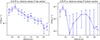 |
Fig. 6. Estimated mass flow rate as a function of the distance along the CF filament structure in G75 (the connecting filament, see red and purple markers in Fig. 1). Left panel: Top section. Right panel: Bottom section. The plots follows the north–south direction from left to right. The velocity differences are taken relative to N1 for the left panel and relative to S1 for the right panel (see annotations). |
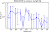 |
Fig. 7. Estimated mass flow rate as a function of the distance along the F-NW filament structure in IRAS21078 (Fig. 1). The graph follows the direction of measurement away from the clump, as indicated by the annotation. |
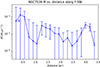 |
Fig. 8. Mass flow rate as a function of the distance along the F-SW filament structure in NGC7538 (Fig. 1). The graph follows the direction of measurement toward the southwest away from S, as indicated by the annotation. |
We chose the main connecting filament in G75 (CF) and the northern and southern halves of the cloud. In IRAS21078, we focused on the three structures that stretch away from the central clump (CC) in northeastern, northwestern, and southwestern direction respectively (Fig. 1). In NGC7538, we picked the northern strip of the cloud, the eastern, and the southwestern structures (Fig. 1). As outlined in the previous section, the data do not directly yield information about the flow direction. Following the picture of dynamical filamentary clouds that collapse and feed star-forming gas clumps (e.g., Myers 2009; Smith et al. 2014, 2016; Vázquez-Semadeni et al. 2019; Padoan et al. 2020) we assume that the flow is always directed toward the clumps. While outflows or expanding HII1.2ex regions might in some region invert the flow direction, for our analysis we assume that the flows are always dominated by accretion flows toward the clumps. Because of this assumption, measurements along structures connecting two clumps were split, where the velocity differences where taken relative to one clump for one half, and relative to the other clump for the other half. This was conducted for CF in G75 and along F-E between IRS9 and S in NGC7538. In order to emphasize this separation, the relevant parts are marked by triangular magenta markers, as seen in Fig. 1. We note that all marker positions were identified by eye. The same holds for the splitting of filaments.
In Fig. 6 we show the mass flow rates along the two halves of CF in G75 (Fig. 1). We can see a characteristic shape of the curve along the structure. While in general the estimated flow rates in this filament decrease with increasing distance to the clump, we note a bump at approximate 2.25–2.75 pc in the plot for the lower part. The same holds for the mass flow rate plot eastward of N2 in G75 (Fig. A.1), where we also observe similar maxima. As for the southern part, the flow rate values from S2 southward show a comparable irregular behavior with increasing distance. As for N2 and S2, we note nearby density enhancements that stand out in the 1.2 mm dust continuum (Fig. 1) and cause a large increase in surface density.
In Fig. 7 we present the estimated mass flow rate along the largest filament structure in IRAS21078, which shows an overall decline in magnitude with increasing distance from the central clump. The mass flow rate does, however, show intriguing peaks at about 0.7, 0.8, and 1.4 pc. We also can see strong depressions at about 0.6 pc and 1.4 pc in Fig. 7.
In Fig. 8 we present the same for the F-SW filament in NGC7538 (cf. Fig. 1), again with declining and peaking mass flow rate estimates along the structure with prominent depressions at about 0.5 to 1.2 pc. All mentioned flow rate increases fall onto the position of overdense sections or minor clumps along filament structures (in comparison to the flow rate graphs with Fig. 1), but at the same time we can also observe velocity gradients in the vicinity of these clumps (see Figs. 2 and 3). The trend of an increasing mass flow rate toward the denser clump sections may therefore be partially associated with an increase in surface density. These sharp maxima along the mass flow rate curve are likely the result of steep velocity differences along the filament.
The mass flow rate estimation along filamentary structures was carried out for all three structures in IRAS21078 (Figs. 7 and A.2) and for the northwestern, eastern, and southwestern structures in NGC7538 (Figs. 8, A.4, A.3). Most of the mass flow plots along filamentary structures show no clear decline in mass flow rate with increasing distance.
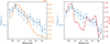 |
Fig. 9. Light blue graph: Mass flow rate as a function of the distance between adjacent points in G75 CF top section (Fig. 1, left panel in Fig. 6). Orange graph, left panel: Surface density along the CF structure top section in G75. Red graph, right panel: Velocity differences along the CF structure top section in G75. |
The important factors contributing to the mass flow rate, the mass surface density Σ and the velocity difference Δv are plotted versus the distance in Figs. 9 and 10 to give a clearer distinction and indicate the more dominant contributor to Ṁ. We can see that the overall shape of the curve is dominated by the surface density for the northern half of the filament and interestingly by the velocity differences for the southern half. Sharp features (i.e., maxima) along the curves stem from strong velocity differences. The possible cause for these velocity differences and the different impacts of the two factors in the top and bottom parts of G75 CF are assessed in Sect. 4.
To be able to compare the correlation of velocity difference and surface density and their impact onto the mass flow rate generally, we plotted the separated factors of Eq. (1) for all major filament structures that we analyze in this sections and present them in Appendix A. Many of the plots show spikes along the curve that either are caused by locally confined overdensities along filaments or steep variations in velocity differences. Most of the curves show a decline in surface density with increasing distance and spikes being caused by Δv (see e.g., Figs. A.7, A.8, A.9, A.10, A.11). In the case of the structure east of N2 in G75, the surface density shows two maxima for two local overdensities (Fig. A.5 and Fig. 1 for reference), but the overall mass flow rate only exhibits a maximum at about 1.7 pc and not at about 0.7 pc, where the velocity difference is low (between 0.2 and 0.3 km s−1 at 0.7 pc compared to about 1 km s−1 at 1.7 pc).
For NGC7538 F-E, the mass flow rate is described by the velocity difference to a large degree (Fig. A.13), whereas a sharp drop in surface density between 0.1 and 0.3 pc does not visibly affect the course of the curve. In the case of the F-NW structure in NGC7538 (Fig. A.11) the HII1.2ex region affects the velocity-distribution of the molecular gas (e.g., Beuther et al. 2022) and thus causing the spikes in the velocity differences, excluding this graph for the accretion-analysis toward IRS1. The same holds for G75 S2 (A.6), where the HII1.2ex region is located nearby between S2 and S1 (see Fig. 1 lower panels). A similar feature appears in the graph for the velocity difference for IRAS21078 F-NE (Fig. A.7), where the sharp maximum at 0.4 pc is located close to the center of the HII1.2ex region (see Fig. 1 bottom panels).
3.3. Flows onto clumps
In order to characterize the gas flow onto the clumps from all directions, the mass flow rates estimated with Eq. (1) are depicted in the form of polar plots for the central massive clumps and star-forming regions to give an intuitive picture of the two-dimensional spatial distribution of mass flow magnitudes. In every polar diagram a red dot is shown as an indicator of the adjacent filament structure. These dots were set by eye. The velocity differences were evaluated by taking the value from one position around the center and subtracting the given velocity value for the center of the clump, similar to our approach along filaments (Section 3.2). The distance Δr in Eq. (1) was set to the half beam size of 13.5″ and the flux values were taken for the same data point as the velocity, in order to be consistent with the previous flow rate approach along the filaments.
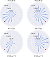 |
Fig. 11. Polar plots showing estimated mass flow rates as a function of the polar angle for the northern clumps in G75 (Fig. 1). Left column: Mass flow rates toward N1, right column: Mass flow rates toward N2. Top panels for the inner circle at 0.36 pc, bottom panels for the outer circle at 0.7 pc. The red dots indicate the direction of the CF filament. |
In this way, the plots always show mass flow rate estimates relative to the center, were 16 individual measurements were conducted (one data point every 22.5 degrees). The radial distances for the measurements were chosen at 20 and 40 arcseconds, resulting in a maximum distance to one clump of about 0.7 pc for G75, 0.52 pc for NGC7538 and 0.29 pc for IRAS21078. Distances farther out exhibit no significant surface density from the dust and are therefore not usable for this polar mass flow rate estimation (cf. Fig. 1).
For this study we investigated prominent clumps of star formation hosted inside the three clouds. The clumps were identified by eye from the dust continuum maps. Their coordinates are given in Table 3. These coordinates were taken from the marker positions toward the clumps (see Fig. 1), which correspond to the peak positions of the dust continuum. For G75, we chose two regions in the northern part of the cloud (N1 and N2, see Fig. 1) and two in the southern part (S1 and S2; see Fig. 1). The two southern clumps are of particular interest since there is a HII1.2ex region between them (see. Fig. 1). In IRAS21078, we evaluated the mass flow behavior at the central part of the cloud (CC; see Fig. 1) and in NGC7538 for IRS1, S, and IRS9 (see Fig. 1). The flow rate estimation around prominent clumps provides further insight into the nature of mass accretion on subparsec scales.
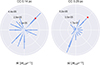 |
Fig. 13. Polar mass flow diagram for the central clump (CC) in IRAS21078 (Fig. 1). Left panel for the inner circle at 0.14 pc; right panel for the outer circle at 0.29 pc. The red dot indicates the direction of the F-NW filament. |
In Fig. 11 we show the flow magnitudes in G75 between 20 and 40 arcseconds spacing for N1 and N2 respectively (cf. Fig. 1). The N1 panel shows a slight orientation toward the filament for both distances, but seems to be more influenced by the eastern direction toward N2 (Fig. 11). The N2 plot depicts a dominating mass flow rate in N1 direction for close proximity, and an increasing contribution from the east for increasing distance. The southern clumps are shown in Fig. 12 without a clear orientation toward CF. Interestingly, S1 shows a strong orientation in mass flow rate magnitude toward S2, and none in direction of CF. S2 on the other hand seems to be primarily influenced from the direction of neighboring S1 and to the west for close proximity. We assume that both S1 and S2 are influenced by the HII1.2ex region in between them (Fig. 1).
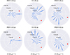 |
Fig. 14. Polar mass flow diagrams for NGC7538 IRS1, S and IRS9 (Fig. 1). Left panels IRS 1, middle panels S and right panels IRS9. Top panels for the inner circle of 0.26 pc; bottom panels for the outer circle at 0.52 pc. Red dots indicate the direction of the F-NW filament (top row for IRS1) and the F-SW filament (bottom row for S). |
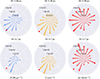 |
Fig. 15. Comparison panels for the clump-centered flow approach. Columns from left to right: Total estimated mass flow rate, surface density and velocity difference for G75 N1 (Fig. 1). Top row: Inner circle at 0.36 pc. Bottom row: Outer circle at 0.7 pc. The red dots indicate adjacent filaments that are assumed to host the potential flow direction. |
The diagram for IRAS21078 is relatively featureless for 0.14 pc distance (Fig. 13), but an increased magnitude of the mass flow rate to the northwest, in the direction of the largest filamentary structure, can be identified. For increasing distance, an influence from the southeastern edge becomes dominant however. The cloud has already been analyzed within the CORE sample and the analysis has shown that it hosts converging flows of material toward its center (Moscadelli et al. 2021). The mass flow direction presented here implies a potential gas infall, but the channeling through the filaments has to be looked at in more detail. Comparing the two-dimensional spatial direction from the mass flow magnitudes in Fig. 13 to the first moment maps in Figs. 2 and 3 shows velocity differences along the structure of HCO+ and H13CO+ prominently in the northwestern direction toward the elongated filament structure. We also note strong HCO+ velocity differences at the southern edge of the cloud (none for H13CO+ because of missing data). This possibly indicates infalling material that is transported laterally onto the structure. The seemingly increasing velocity gradient toward blueshifted gas at more densely packed contour lines of the dust continuum may indicate increasing dynamics due to channeling of the material closer to the center. This is speculative, however, as this assessment largely rests upon the HCO+ and H13CO+ first moment maps alone. One always has to consider the presence of the HII1.2ex regions, which likely cause alterations in potential gravitationally driven infall via feedback processes. This should be noted especially for IRAS21078, where the extent of the HII1.2ex region covers almost the whole source (Fig. 1 lower panel).
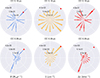 |
Fig. 16. Comparison panels for the clump-centered flow approach. Columns from left to right: Total estimated mass flow rate, surface density and velocity difference for IRAS21078 CC (Fig. 1). Top row: Inner circle at 0.14 pc. Bottom row: Outer circle at 0.29 pc. The red dots indicate adjacent filaments that are assumed to host the potential flow direction. |
For NGC7538, we can see the diagrams for IRS1, S and IRS9 clumps in Fig. 14 (for reference, see Fig. 1). IRS1 shows more extended flow magnitudes toward the west in the direction of the F-NW filament, which declines for increasing distance (about 0.52 pc), but remains the dominant value. This probably can be explained by a strong velocity difference in the H13CO+ data (Fig. 3). S indicates a more prominent flow direction toward the northern IRS1, especially for a 0.52 pc distance. It is interesting to note that S seems to be influenced by IRS1, but not vice versa. Assuming that the northern HII1.2ex region may have triggered the formation of IRS1, this region should be slightly older than S. Hence, influence of IRS1 on S but not the other way round appears plausible. The mass flow magnitude toward S also yields no visible influence from the F-SW filament structure. For IRS9, both distances depict almost the same pattern: the flow rate direction is concentrated to the southern half of the circle; there is a more obvious contribution from the eastern section than from the filament connecting IRS9 with S (Fig. 1).
In order to obtain a more precise overview of the contributors to the mass flow rate (Eq. (1)), we conducted the same separation for Σ and Δv as in Section 3.2. We present the comparison panels for G75 N1 in Fig. 15, for IRAS21078 CC in Fig. 16 and for NGC7538 IRS1 in Fig. 17. The diagrams for all the other clumps are shown in Appendix B.
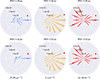 |
Fig. 17. Comparison panels for the clump-centered flow approach. Columns from left to right: Total estimated mass flow rate, surface density and velocity difference for NGC7538 IRS1 (Fig. 1). Top row: Inner circle at 0.26 pc. Bottom row: Outer circle at 0.52 pc. The red dots indicate adjacent filaments that are assumed to host the potential flow direction. |
For the most part, the velocity differences appear to have a more dominant impact on the shape of the polar magnitude-distribution. For clump G75 N1 (Fig. 15), however, the surface density seems to be the strongest contributor. For example, we can see that the strong flow rates in G75 S1 are dominated by the velocity difference toward S2 (Fig. B.2), while the surface density is orientated toward the east and does not align at all with the expected filament direction (red dot) and only to a small degree with the velocity differences. The same holds for S2 toward S1 (Fig. B.3). IRAS21078 CC exhibits one spike in the F-NW direction that clearly stems from the velocity difference due to the close distance (Fig. 16). The same holds for the outer annulus, where the surface density now points in the F-NW direction, but the velocity difference toward the southeast is stronger and thus affects the overall mass flow to a larger degree. This also is visible for NGC7538S (Fig. B.4).
As we summarize in Fig. 18, the peak values for all of the mass flow rates occur in the outer annulus of 40″. This indicates that a larger fraction of mass is transported toward the clumps on a larger scale.
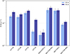 |
Fig. 18. Peak values of the estimated mass flow rate toward clumps. The light blue bars show the values for the 20″ distance, while the dark blue bars show values for the 40″ distance. The error bars show the maximum error of the respective mass flow rate. We note that this chart shows the maximum values of Ṁ alone, and contains no information about the direction from the polar plots. |
4. Discussion, conclusions, and summary
In this paper we analyzed the kinematics of molecular gas in three high-mass star-forming molecular clouds. In order to do this, we estimated the mass flow rates and divided the analysis into mass flows along filamentary structures and flows onto clumps. Both approaches indicate that mass is transported along these structures. Along filamentary cloud structures, we find increasing mass flow magnitudes close to denser regions. The peak values are on the order of 10−3 M⊙ for G75 and 10−5 M⊙ and 10−4 M⊙ for IRAS21078 and NGC7538, respectively. As given in Table 3, we note that IRAS21078 is a lower mass clump which therefore exhibits the lowest overall mass flow rate.
The analysis of the flows onto clumps focused on the interpretation of polar diagrams, that show the orientation of the mass flow rate magnitude toward a clump. In G75, the direction of the strongest mass flow rate indicates a potential feeding of the northern half of the cloud through the central connecting filament structure. Similar patterns appear in NGC7538 for the two clumps IRS1 and S. For IRAS21078, the distribution of the flow rates indicates an infall from the northwestern filament structure, but one has to bear in mind the comparably large errors; however, it appears possible that the infall of material through these channels occurs. This has already been the subject of studies on smaller spatial scales, with similar findings.
The separation of the two main contributors to the mass flow rates into velocity difference and surface density showed interesting patterns for both methods: for the flows along the G75 CF structure, the surface density dictates the overall shape of the curve; on the other hand, spikes are contributed by steep velocity differences. Sharp increases in velocity differences often affect the mass flow curve to a large degree, and the data indicate that they often stem from feedback from the HII1.2ex regions. In the case of the polar diagrams, the orientation of the surface density toward filament structures was sometimes not visible due to a strong velocity difference into a different direction. There are cases however, where the two factors of the mass flow rate equation are more aligned. This is very interesting since an orientated distribution of dust for close proximity might hint at channel or filament structures that serve as a gas funnel. The fact that the larger velocity differences sometimes do not point toward adjacent clumps or in filament direction might be caused by expanding shells from nearby HII1.2ex regions; this very likely is the case for G75 S1 and S2. For the clumps were we also found velocity differences in the filament directions, we can assume that it potentially is accretionally driven through the filaments. For the regions where this behavior does not occur, we can tentatively infer that the HII1.2ex regions are responsible due to feedback processes: this assessment is supported by the fact that all clumps that show flow rate magnitudes in unexpected directions in the polar plots are located close to a HII1.2ex region.
Similar to the assertion of a dominant contributor in the mass flow rate, large flow-magnitude values close to the edge of a cloud (cf. Fig. 14) do not necessarily imply increasing dynamics in the gas flow, but could just be a consequence of the steep gradient in the surface density profile (cf. Eq. (1) and Fig. 1, especially in the vicinity of IRS1 and IRS9 in NGC7538 that are located close to the edge of the 1.2 mm dust emission).
If we assume that the accretion is mainly gravitationally driven close to denser regions (e.g., clumps), the material should fall onto the clumps; driving mechanisms such as turbulence on larger scales have been numerically studied by Padoan et al. 2020, among others. Large-scale infall would precede the fragmentation of the cloud and further collapse of protostars that exceed their individual Jeans mass (Vázquez-Semadeni et al. 2019). In the case of the regions presented here, we find strong indications for feedback processes to be the driving force behind gas dynamics in the clouds. The regions with a HII1.2ex region can differ in their behavior, and the plots indicate that they certainly do. Their influence is strongly noticeable in the disrupted flow behavior and the lack of molecular line data (Fig. 1). For this reason, especially the northwestern part of NGC7538 has to be excluded from the accretion flow assessment in general due to the HII1.2ex region (e.g., Beuther et al. 2022) (see also Sect. 3 and Fig. 1). Filaments appear at the boundaries of HII1.2ex regions in all presented sources with strong indications for increased mass flow. This supports the simulations predicting filament formation at the crossing of shocks (e.g., Pudritz & Kevlahan 2013). We only included the analysis for the HCO+ and H13CO+ molecules in the main section since the other molecules that exhibit a similar spatial distribution (e.g., HCN and H2CO) did not yield additional information in their apparent kinematics.
For further information, see https://www.iram.fr/IRAMFR/GILDAS/
Acknowledgments
This work is based on observations carried out under project number 121-20 with the IRAM 30m telescope. IRAM is supported by INSU/CNRS (France), MPG (Germany) and IGN (Spain). A.P. acknowledges financial support from the UNAM-PAPIIT IG100223 grant, the Sistema Nacional de Investigadores of SECIHTI, and from the SECIHTI project number 86372 of the ‘Ciencia de Frontera 2019’ program, entitled ‘Citlalcóatl: A multiscale study at the new frontier of the formation and early evolution of stars and planetary systems’, México. S.F. acknowledges support from the National Key R&D program of China grant (2025YFE0108200), National Science Foundation of China (12373023, 1213308).
References
- Ahmadi, A., Beuther, H., Bosco, F., et al. 2023, A&A, 677, A171 [NASA ADS] [CrossRef] [EDP Sciences] [Google Scholar]
- Ando, K., Nagayama, T., Omodaka, T., et al. 2011, PASJ, 63, 45 [NASA ADS] [Google Scholar]
- Beuther, H., et al. 2020, A&A, 638, A44 [NASA ADS] [CrossRef] [EDP Sciences] [Google Scholar]
- Beuther, H., Mottram, J. C., Ahmadi, A., et al. 2018, A&A, 617, A100 [NASA ADS] [CrossRef] [EDP Sciences] [Google Scholar]
- Beuther, H., Schneider, N., Simon, R., et al. 2022, A&A, 659, A77 [NASA ADS] [CrossRef] [EDP Sciences] [Google Scholar]
- Beuther, H., Gieser, C., Soler, J. D., et al. 2024, A&A, 682, A81 [NASA ADS] [CrossRef] [EDP Sciences] [Google Scholar]
- Condon, J. J., Cotton, W. D., Greisen, E. W., et al. 1998, AJ, 115, 1693 [Google Scholar]
- Draine, B. T. 2011, Physics of the Interstellar and Intergalactic Medium (Princeton University Press) [Google Scholar]
- Federrath, C., & Klessen, R. S. 2012, ApJ, 761, 156 [Google Scholar]
- Gieser, C., Beuther, H., Semenov, D., et al. 2021, A&A, 648, A66 [EDP Sciences] [Google Scholar]
- Gieser, C., Beuther, H., Semenov, D., et al. 2023, A&A, 674, A160 [NASA ADS] [CrossRef] [EDP Sciences] [Google Scholar]
- Hacar, A., Clark, S. E., Heitsch, F., et al. 2023, in Protostars and Planets VII, eds. S. Inutsuka, Y. Aikawa, T. Muto, K. Tomida, & M. Tamura, ASP Conf. Ser., 534, 153 [NASA ADS] [Google Scholar]
- Hennebelle, P., & Chabrier, G. 2011, ApJ, 743, L29 [Google Scholar]
- Hildebrand, R. H. 1983, QJRAS, 24, 267 [NASA ADS] [Google Scholar]
- Jiao, S., Lin, Y., Shui, X., et al. 2022, Sci. China Phys. Mech. Astron., 65, 299511 [NASA ADS] [CrossRef] [Google Scholar]
- Kim, S., Lee, C. W., Tafalla, M., et al. 2022, ApJ, 940, 112 [NASA ADS] [CrossRef] [Google Scholar]
- Krumholz, M. R., McKee, C. F., & Klein, R. I. 2005, ApJ, 618, L33 [NASA ADS] [CrossRef] [Google Scholar]
- Lin, Y., Liu, H. B., Li, D., et al. 2016, ApJ, 828, 32 [NASA ADS] [CrossRef] [Google Scholar]
- Ma, Y., Zhou, J., Esimbek, J., et al. 2023, A&A, 676, A15 [NASA ADS] [CrossRef] [EDP Sciences] [Google Scholar]
- Mac Low, M.-M., & Klessen, R. S. 2004, Rev. Mod. Phys., 76, 125 [Google Scholar]
- Marsh, K. A., Whitworth, A. P., Lomax, O., et al. 2017, MNRAS, 471, 2730 [Google Scholar]
- Molinari, S., Brand, J., Cesaroni, R., & Palla, F. 1996, A&A, 308, 573 [NASA ADS] [Google Scholar]
- Molinari, S., Swinyard, B., Bally, J., et al. 2010, A&A, 518, L100 [NASA ADS] [CrossRef] [EDP Sciences] [Google Scholar]
- Molinari, S., Schisano, E., Elia, D., et al. 2016, A&A, 591, A149 [NASA ADS] [CrossRef] [EDP Sciences] [Google Scholar]
- Moscadelli, L., Reid, M. J., Menten, K. M., et al. 2009, ApJ, 693, 406 [NASA ADS] [CrossRef] [Google Scholar]
- Moscadelli, L., Beuther, H., Ahmadi, A., et al. 2021, A&A, 647, A114 [EDP Sciences] [Google Scholar]
- Myers, P. C. 2009, ApJ, 700, 1609 [Google Scholar]
- Ossenkopf, V., & Henning, T. 1994, A&A, 291, 943 [NASA ADS] [Google Scholar]
- Padoan, P., & Nordlund, Å. 2011, ApJ, 730, 40 [Google Scholar]
- Padoan, P., Pan, L., Juvela, M., Haugbølle, T., & Nordlund, Å. 2020, ApJ, 900, 82 [NASA ADS] [CrossRef] [Google Scholar]
- Peretto, N., Fuller, G. A., Duarte-Cabral, A., et al. 2013, A&A, 555, A112 [NASA ADS] [CrossRef] [EDP Sciences] [Google Scholar]
- Peretto, N., Fuller, G. A., André, P., et al. 2014, A&A, 561, A83 [NASA ADS] [CrossRef] [EDP Sciences] [Google Scholar]
- Perotto, L., Ponthieu, N., Macías-Pérez, J. F., et al. 2020, A&A, 637, A71 [NASA ADS] [CrossRef] [EDP Sciences] [Google Scholar]
- Pineda, J. E., Arzoumanian, D., Andre, P., et al. 2023, in Protostars and Planets VII, eds. S. Inutsuka, Y. Aikawa, T. Muto, K. Tomida, & M. Tamura, ASP Conf. Ser., 534, 233 [NASA ADS] [Google Scholar]
- Pudritz, R. E., & Kevlahan, N. K. R. 2013, Philos. Trans. R. Soc. London Ser. A, 371, 20120248 [Google Scholar]
- Puga, E., Marín-Franch, A., Najarro, F., et al. 2010, A&A, 517, A2 [NASA ADS] [CrossRef] [EDP Sciences] [Google Scholar]
- Reid, M. J., Menten, K. M., Zheng, X. W., et al. 2009, ApJ, 700, 137 [CrossRef] [Google Scholar]
- Riffel, R. A., & Lüdke, E. 2014, Adv. Astron., 2014, 192513 [Google Scholar]
- Schuller, F., Menten, K. M., Contreras, Y., et al. 2009, A&A, 504, 415 [NASA ADS] [CrossRef] [EDP Sciences] [Google Scholar]
- Shirley, Y. L. 2015, PASP, 127, 299 [Google Scholar]
- Smith, R. J., Shetty, R., Stutz, A. M., & Klessen, R. S. 2012, ApJ, 750, 64 [NASA ADS] [CrossRef] [Google Scholar]
- Smith, R. J., Glover, S. C. O., & Klessen, R. S. 2014, MNRAS, 445, 2900 [Google Scholar]
- Smith, R. J., Glover, S. C. O., Klessen, R. S., & Fuller, G. A. 2016, MNRAS, 455, 3640 [Google Scholar]
- Vázquez-Semadeni, E., Ballesteros-Paredes, J., & Klessen, R. 2003, in Galactic Star Formation Across the Stellar Mass Spectrum, eds. J. M. De Buizer, & N. S. van der Bliek, ASP Conf. Ser., 287, 81 [Google Scholar]
- Vázquez-Semadeni, E., Palau, A., Ballesteros-Paredes, J., Gómez, G. C., & Zamora-Avilés, M. 2019, MNRAS, 490, 3061 [Google Scholar]
- Wells, M. R. A., Beuther, H., Molinari, S., et al. 2024, A&A, 690, A185 [NASA ADS] [CrossRef] [EDP Sciences] [Google Scholar]
- Zhao, B., Pudritz, R. E., Pillsworth, R., Robinson, H., & Wadsley, J. 2024, ApJ, 974, 240 [NASA ADS] [CrossRef] [Google Scholar]
Appendix A: Additional mass flow and comparison graphs (along filaments)
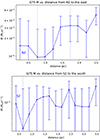 |
Fig. A.1. Top: Estimated mass flow rate as a function of the distance from N2 eastward in G75 (see Fig. 1). The blue graph follows the west–east direction starting at N2 from left to right. The dotted blue lines mark the approximate positions of the density enhancements along the structure. Bottom: Same but for S2. |
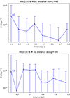 |
Fig. A.2. Top: Mass flow estimates as a function of distance (of adjacent points) along the F-NE filament structure in IRAS21078 (cf. Fig. 1). The direction of measurement is from the clump outward, where CC indicates the starting point. Bottom: The same for F-SW. |
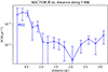 |
Fig. A.3. Mass flow estimates as a function of distance (of adjacent points) along the F-NW filament structure in NGC7538 (cf. Fig. 1). |
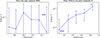 |
Fig. A.4. Mass flow estimates as a function of distance (of adjacent points) along the F-E filament structure in NGC7538. The panels are aligned such that the direction of measurement can be traced directly from Fig. 1. |
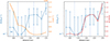 |
Fig. A.5. Light blue graph: Mass flow rate as a function of the distance between adjacent points in G75 from N2 eastward (Fig. 1). Orange graph, left panel: Surface density in G75 from N2 eastward. Red graph, right panel: Velocity differences in G75 from N2 eastward. The dotted blue lines mark the approximate positions of the density enhancements along the structure. |
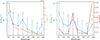 |
Fig. A.7. Light blue graph: Mass flow rate as a function of the distance between adjacent points in IRAS21078 F-NE (Fig. 1). Orange graph, left panel: Surface density along the F-NE-structure in IRAS21078. Red graph, right panel: Velocity differences along the F-NE-structure in IRAS21078. |
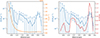 |
Fig. A.10. Light blue graph: Mass flow rate as a function of the distance between adjacent points in NGC7538 F-SW (Fig. 1). Orange graph, left panel: Surface density along the F-SW-structure in NGC7538. Red graph, right panel: Velocity differences along the F-SW-structure in NGC7538. |
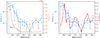 |
Fig. A.11. Same as Fig. A.10 but for NGC7538 F-NW. |
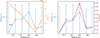 |
Fig. A.12. Same as Fig. A.10 but for NGC7538 F-E (from IRS9 toward the east). |
 |
Fig. A.13. Same as Fig. A.12 but from NGC7538 IRS9 toward S. |
Appendix B: Additional comparison graphs (polar diagrams)
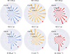 |
Fig. B.1. Comparison panels for the clump-centered flow approach. Columns from left to right: Total estimated mass flow rate, surface density, and velocity difference for G75 N2 (Fig. 1). The red dots indicate adjacent filaments, which are assumed to host the potential flow direction. |
Appendix C: Moment zero maps and emission spectra
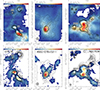 |
Fig. C.1. Top: Moment zero (integrated intensity) maps for the HCO+ (1 − 0) line. The beam size is 27″ (lower left corner). The scale bar indicates the length of 1 parsec in each panel. The contour lines show the 1.2 mm dust continuum ranging from 3σ to 39σ in 3σ steps. Bottom: Same for H13CO+ (1 − 0). |
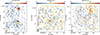 |
Fig. C.2. Moment zero maps of the H41α recombination line tracing the free–free contribution. The black contours outline the free–free corrected 1.2 mm dust continuum (except for IRAS21078) on log-scale starting from 5σ (except for IRAS21078 starting from 3σ) to peak value for reference. For G75 (left panel) and NGC7538 (right panel) the strongest emission fits the contours in the lower panels of Fig. 1; for IRAS21078 (middle panel) there is only noise and no significant contribution from the HII1.2ex region outlined in NVSS. The edges have been set to values of zero in order to eliminate the stripe artifacts from the OTF scanning process. All blank spots represent zero values due to the log-scaling. |
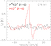 |
Fig. C.3. Molecular emission in G75 N1. Due to the lack of H13CO+ emission close to N1, we widened the search radius from 10″ to 30″. |
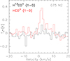 |
Fig. C.4. Molecular emission in G75 N2. |
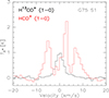 |
Fig. C.5. Molecular emission in G75 S1. |
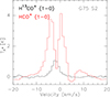 |
Fig. C.6. Molecular emission in G75 S2. |
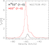 |
Fig. C.7. Molecular emission in NGC7538 IRS1. |
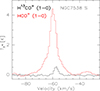 |
Fig. C.8. Molecular emission in NGC7538 S. |
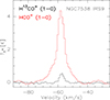 |
Fig. C.9. Molecular emission in NGC7538 IRS9. |
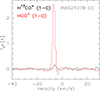 |
Fig. C.10. Molecular emission in IRAS21078 CC. |
All Tables
Overview of the molecular properties for the two molecules presented in this paper.
Overview of σrms values of the molecular transitions at a spectral resolution of 0.9 km s−1.
Peak- and σrms values of the 1.2 mm dust continuum and the 1.4 GHz (21 cm) data (HII1.2ex regions).
All Figures
|
Fig. 1. Top row: NIKA2 1.2 mm dust continuum maps (see Beuther et al. 2024) of the star-forming regions showing the clump and filament designations. The red and magenta markers indicate the data points used for the flow rate estimation in Section 3.2. The triangular magenta markers indicate a separate section along a structure. Black contours outline the 1.2 mm continuum, ranging from 3σ to 39σ in steps of 3σ (the RMS values are presented in Table 5). The red contours in the upper panels mark the peak positions of the continuum emission from 20% to 100% in steps of 20%. The designations used in the following refer to clumps and filament structures, filaments are labeled F; CF in G75 is the central filament; CC in IRAS21078 is the central clump. The clumps in NGC7538 are the known objects IRS9, IRS1 and S (e.g., Beuther 2020). G75 S1 is the object G75.78+0.34. We present the clump designations together with their coordinates in Table 3. Bottom row: Same dust-maps, but with red contour lines outlining the HII1.2ex regions at 1.4 GHz (21 cm) (Condon et al. 1998); the contours range from 10% to 100% of the peak emission in steps of 10% (see Table 5 for reference). The positions of the two main exciting sources of the HII1.2ex region in NGC7538, NGC7538 IRS5 and NGC7538 IRS6, are marked in the lower right panel (Puga et al. 2010). |
| In the text | |
|
Fig. 2. First moment (intensity-weighted peak velocity) maps for the HCO+ (1 − 0) line. The beam size is 27″ (lower left corner). The sources are labeled in each panel. The scale bar indicates the length of 1 parsec in each panel. The contour lines show the 1.2 mm dust continuum ranging from 3σ to 39σ in 3σ steps. |
| In the text | |
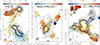 |
Fig. 3. Same as Fig. 2 but for the H13CO+ (1 − 0)-transition. |
| In the text | |
|
Fig. 4. Dust temperature maps of G75 (left panel) and NGC7538 (right panel). Both maps were created using Herschel data (Molinari et al. 2010) and free–free corrected dust continuum emission from the NIKA2 dataset. In the bottom left corner the 27″ beam of the final data product is shown. The black contours outline the free–free corrected 1.2 mm continuum emission at 27″ resolution in logarithmic scale from 5σ to peak value. |
| In the text | |
|
Fig. 5. Spectra toward G75 showing molecular emission of HCO+ (1 − 0) (red) and H13CO+ (1 − 0) (black). The left panel shows the emission at the clump position S1 in G75. The right panel shows the spectra for a position along the CF filament in G75 (see upper left panel of Fig. 1). |
| In the text | |
|
Fig. 6. Estimated mass flow rate as a function of the distance along the CF filament structure in G75 (the connecting filament, see red and purple markers in Fig. 1). Left panel: Top section. Right panel: Bottom section. The plots follows the north–south direction from left to right. The velocity differences are taken relative to N1 for the left panel and relative to S1 for the right panel (see annotations). |
| In the text | |
|
Fig. 7. Estimated mass flow rate as a function of the distance along the F-NW filament structure in IRAS21078 (Fig. 1). The graph follows the direction of measurement away from the clump, as indicated by the annotation. |
| In the text | |
|
Fig. 8. Mass flow rate as a function of the distance along the F-SW filament structure in NGC7538 (Fig. 1). The graph follows the direction of measurement toward the southwest away from S, as indicated by the annotation. |
| In the text | |
|
Fig. 9. Light blue graph: Mass flow rate as a function of the distance between adjacent points in G75 CF top section (Fig. 1, left panel in Fig. 6). Orange graph, left panel: Surface density along the CF structure top section in G75. Red graph, right panel: Velocity differences along the CF structure top section in G75. |
| In the text | |
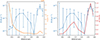 |
Fig. 10. Same as Fig. 9 but for the CF bottom section. |
| In the text | |
|
Fig. 11. Polar plots showing estimated mass flow rates as a function of the polar angle for the northern clumps in G75 (Fig. 1). Left column: Mass flow rates toward N1, right column: Mass flow rates toward N2. Top panels for the inner circle at 0.36 pc, bottom panels for the outer circle at 0.7 pc. The red dots indicate the direction of the CF filament. |
| In the text | |
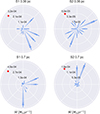 |
Fig. 12. Same as Fig. 11 but for the southern clumps. |
| In the text | |
|
Fig. 13. Polar mass flow diagram for the central clump (CC) in IRAS21078 (Fig. 1). Left panel for the inner circle at 0.14 pc; right panel for the outer circle at 0.29 pc. The red dot indicates the direction of the F-NW filament. |
| In the text | |
|
Fig. 14. Polar mass flow diagrams for NGC7538 IRS1, S and IRS9 (Fig. 1). Left panels IRS 1, middle panels S and right panels IRS9. Top panels for the inner circle of 0.26 pc; bottom panels for the outer circle at 0.52 pc. Red dots indicate the direction of the F-NW filament (top row for IRS1) and the F-SW filament (bottom row for S). |
| In the text | |
|
Fig. 15. Comparison panels for the clump-centered flow approach. Columns from left to right: Total estimated mass flow rate, surface density and velocity difference for G75 N1 (Fig. 1). Top row: Inner circle at 0.36 pc. Bottom row: Outer circle at 0.7 pc. The red dots indicate adjacent filaments that are assumed to host the potential flow direction. |
| In the text | |
|
Fig. 16. Comparison panels for the clump-centered flow approach. Columns from left to right: Total estimated mass flow rate, surface density and velocity difference for IRAS21078 CC (Fig. 1). Top row: Inner circle at 0.14 pc. Bottom row: Outer circle at 0.29 pc. The red dots indicate adjacent filaments that are assumed to host the potential flow direction. |
| In the text | |
|
Fig. 17. Comparison panels for the clump-centered flow approach. Columns from left to right: Total estimated mass flow rate, surface density and velocity difference for NGC7538 IRS1 (Fig. 1). Top row: Inner circle at 0.26 pc. Bottom row: Outer circle at 0.52 pc. The red dots indicate adjacent filaments that are assumed to host the potential flow direction. |
| In the text | |
|
Fig. 18. Peak values of the estimated mass flow rate toward clumps. The light blue bars show the values for the 20″ distance, while the dark blue bars show values for the 40″ distance. The error bars show the maximum error of the respective mass flow rate. We note that this chart shows the maximum values of Ṁ alone, and contains no information about the direction from the polar plots. |
| In the text | |
|
Fig. A.1. Top: Estimated mass flow rate as a function of the distance from N2 eastward in G75 (see Fig. 1). The blue graph follows the west–east direction starting at N2 from left to right. The dotted blue lines mark the approximate positions of the density enhancements along the structure. Bottom: Same but for S2. |
| In the text | |
|
Fig. A.2. Top: Mass flow estimates as a function of distance (of adjacent points) along the F-NE filament structure in IRAS21078 (cf. Fig. 1). The direction of measurement is from the clump outward, where CC indicates the starting point. Bottom: The same for F-SW. |
| In the text | |
|
Fig. A.3. Mass flow estimates as a function of distance (of adjacent points) along the F-NW filament structure in NGC7538 (cf. Fig. 1). |
| In the text | |
|
Fig. A.4. Mass flow estimates as a function of distance (of adjacent points) along the F-E filament structure in NGC7538. The panels are aligned such that the direction of measurement can be traced directly from Fig. 1. |
| In the text | |
|
Fig. A.5. Light blue graph: Mass flow rate as a function of the distance between adjacent points in G75 from N2 eastward (Fig. 1). Orange graph, left panel: Surface density in G75 from N2 eastward. Red graph, right panel: Velocity differences in G75 from N2 eastward. The dotted blue lines mark the approximate positions of the density enhancements along the structure. |
| In the text | |
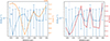 |
Fig. A.6. Same as Fig. A.5 but for S2. |
| In the text | |
|
Fig. A.7. Light blue graph: Mass flow rate as a function of the distance between adjacent points in IRAS21078 F-NE (Fig. 1). Orange graph, left panel: Surface density along the F-NE-structure in IRAS21078. Red graph, right panel: Velocity differences along the F-NE-structure in IRAS21078. |
| In the text | |
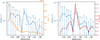 |
Fig. A.8. Same as Fig. A.7 but for IRAS21078 F-NW. |
| In the text | |
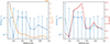 |
Fig. A.9. Same as Fig. A.7 but for IRAS21078 F-SW. |
| In the text | |
|
Fig. A.10. Light blue graph: Mass flow rate as a function of the distance between adjacent points in NGC7538 F-SW (Fig. 1). Orange graph, left panel: Surface density along the F-SW-structure in NGC7538. Red graph, right panel: Velocity differences along the F-SW-structure in NGC7538. |
| In the text | |
|
Fig. A.11. Same as Fig. A.10 but for NGC7538 F-NW. |
| In the text | |
|
Fig. A.12. Same as Fig. A.10 but for NGC7538 F-E (from IRS9 toward the east). |
| In the text | |
|
Fig. A.13. Same as Fig. A.12 but from NGC7538 IRS9 toward S. |
| In the text | |
|
Fig. B.1. Comparison panels for the clump-centered flow approach. Columns from left to right: Total estimated mass flow rate, surface density, and velocity difference for G75 N2 (Fig. 1). The red dots indicate adjacent filaments, which are assumed to host the potential flow direction. |
| In the text | |
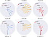 |
Fig. B.2. Same as Fig. B.1 but for G75 S1. |
| In the text | |
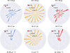 |
Fig. B.3. Same as Fig. B.1 but for G75 S2. |
| In the text | |
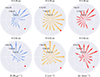 |
Fig. B.4. Same as Fig. B.1 but for NGC7538 S. |
| In the text | |
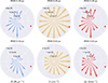 |
Fig. B.5. Same as Fig. B.1 but for NGC7538 IRS9. |
| In the text | |
|
Fig. C.1. Top: Moment zero (integrated intensity) maps for the HCO+ (1 − 0) line. The beam size is 27″ (lower left corner). The scale bar indicates the length of 1 parsec in each panel. The contour lines show the 1.2 mm dust continuum ranging from 3σ to 39σ in 3σ steps. Bottom: Same for H13CO+ (1 − 0). |
| In the text | |
|
Fig. C.2. Moment zero maps of the H41α recombination line tracing the free–free contribution. The black contours outline the free–free corrected 1.2 mm dust continuum (except for IRAS21078) on log-scale starting from 5σ (except for IRAS21078 starting from 3σ) to peak value for reference. For G75 (left panel) and NGC7538 (right panel) the strongest emission fits the contours in the lower panels of Fig. 1; for IRAS21078 (middle panel) there is only noise and no significant contribution from the HII1.2ex region outlined in NVSS. The edges have been set to values of zero in order to eliminate the stripe artifacts from the OTF scanning process. All blank spots represent zero values due to the log-scaling. |
| In the text | |
|
Fig. C.3. Molecular emission in G75 N1. Due to the lack of H13CO+ emission close to N1, we widened the search radius from 10″ to 30″. |
| In the text | |
|
Fig. C.4. Molecular emission in G75 N2. |
| In the text | |
|
Fig. C.5. Molecular emission in G75 S1. |
| In the text | |
|
Fig. C.6. Molecular emission in G75 S2. |
| In the text | |
|
Fig. C.7. Molecular emission in NGC7538 IRS1. |
| In the text | |
|
Fig. C.8. Molecular emission in NGC7538 S. |
| In the text | |
|
Fig. C.9. Molecular emission in NGC7538 IRS9. |
| In the text | |
|
Fig. C.10. Molecular emission in IRAS21078 CC. |
| In the text | |
Current usage metrics show cumulative count of Article Views (full-text article views including HTML views, PDF and ePub downloads, according to the available data) and Abstracts Views on Vision4Press platform.
Data correspond to usage on the plateform after 2015. The current usage metrics is available 48-96 hours after online publication and is updated daily on week days.
Initial download of the metrics may take a while.