| Issue |
A&A
Volume 705, January 2026
|
|
|---|---|---|
| Article Number | A53 | |
| Number of page(s) | 19 | |
| Section | Extragalactic astronomy | |
| DOI | https://doi.org/10.1051/0004-6361/202556147 | |
| Published online | 06 January 2026 | |
MEGADES: MEGARA galaxy disc evolution survey
Ionised gas diagnosis
1
Departamento de Física de la Tierra y Astrofísica, Universidad Complutense de Madrid, E-28040 Madrid, Spain
2
Instituto de Física de Partículas y del Cosmos IPARCOS, Facultad de Ciencias Físicas, Universidad Complutense de Madrid, E-28040 Madrid, Spain
3
Instituto Nacional de Astrofísica, Óptica y Electrónica, Luis Enrique Erro No.1, C.P. 72840 Tonantzintla, Puebla, Mexico
4
Instituto de Astrofísica de Andalucía-CSIC, Glorieta de la Astronomía s/n, 18008 Granada, Spain
5
Universidad Politécnica de Madrid, Madrid, Spain
6
FRACTAL S.L.N.E. C/ Tulipán 2, p13, 1A. E-28231 Las Rozas de Madrid, Spain
★ Corresponding author: This email address is being protected from spambots. You need JavaScript enabled to view it.
Received:
27
June
2025
Accepted:
17
October
2025
Abstract
We present the ionised gas properties and metallicity gradients of the central area of a sample of 43 galaxies using observations obtained by the MEGADES survey. The technical capabilities of MEGARA (Multi-Espectrógrafo en GTC de Alta Resolución para Astronomía) provide us with relatively high spectral (R ∼ 6000) and spatial (0.62″) resolution observations that we used to study the properties of the ionised gas via various methods, including using the classic diagnostic BPT diagrams of its [N II] and [S II] variants. We explore how the diagrams vary as a function of both the radius and velocity dispersion of the Hα line. We also propose a new diagnostic diagram for assessing the relative contributions of active galactic nuclei (AGN), shocks, and H II regions in each spatial region as the ratio between the velocity dispersion of the [N II]λ6584 and Hα lines. A considerable number of regions, regardless of their galactocentric distance, have emission line spectra associated with shocks. This inference follows both from their line ratios, typically characterised by high [N II]λ6584/Hα and intermediate [O III]λ5007/Hβ, and from their position in our diagnostic diagram, where they lie between the areas associated with HII regions and with AGN. The better selection of HII-region-like emission allowed for a robust oxygen abundance determination using the N2 indicator, which we used to measure precise abundance gradients. Most galaxies show negligible metallicity gradients, especially the low-abundance (< 8.37 dex) fast rotators. The mean value of the slope of the metallicity gradients for this subset is 0.005 dex Re−1, with a dispersion of 0.422 dex Re−1. Above 8.37 dex the fast rotators consistently show slightly negative metallicity gradients, with a weak correlation between the slope and the y-intercept. The mean slope of these galaxies is −0.681 dex Re−1, with a dispersion of 0.933 dex Re−1. The overall mean value of the gradients for all galaxies in the MEGADES sample is −0.025 dex Re−1, with a dispersion of 0.766 dex Re−1. We discuss the possible implications of these results regarding the impact of galactic winds on the abundance gradients of galaxies.
Key words: galaxies: ISM / galaxies: star formation
© The Authors 2026
 Open Access article, published by EDP Sciences, under the terms of the Creative Commons Attribution License (https://creativecommons.org/licenses/by/4.0), which permits unrestricted use, distribution, and reproduction in any medium, provided the original work is properly cited.
This article is published in open access under the Subscribe to Open model. This email address is being protected from spambots. You need JavaScript enabled to view it. to support open access publication.
1. Introduction
The emission spectra of galaxies are a treasure trove of information that can be exploited to measure several physical parameters of the interstellar medium (ISM), including the gas density, temperature, ionisation, and abundance. The precise properties of the ISM can be determined with detailed photoionisation models such as Cloudy (Ferland et al. 1998), PyNeb (Luridiana et al. 2015), MAPPINGS (Sutherland et al. 2018), and HCm (Pérez-Montero 2014), which calculate the proper energy balance between atomic species and the energy levels of each species. Most of the time, however, it is far more practical or even only possible to use line emission diagnostics based on strong emission lines, which are easy to measure with significant signal-to-noise ratios (S/Ns; e.g. Kewley & Dopita 2002; Marino et al. 2013; Pilyugin & Grebel 2016; Curti et al. 2017).
These line emission diagnostics have become one of the main tools employed in extragalactic astronomy studies aimed at understanding the physics of galaxies. A multitude of particular diagnostic applications can be used, which provide information on virtually any relevant physical parameter of the ISM of the galaxies (see reviews by Kewley et al. 2019 and Maiolino & Mannucci 2019). One of the most used diagnostics is the Baldwin, Phillips, and Terlevich (BPT) diagram (Baldwin et al. 1981), which is based on the Hα, Hβ, [N II], and [O III] emission lines ([N II] can be substituted by [S II] and [O I] lines). In this diagram, the combination of lines informs the user of the hardness of the ionising spectra acting on the ISM as well as how prevalent shocks are as an ionisation source. The BPT diagram allows for the classification of galaxies (or regions within them) by the origin of the ionisation and, consequently, the emission that is observed, which is tied to physical processes such as star-forming-region-based ionisation by young massive stars, active galactic nucleus (AGN) feedback, or ionisation by old stellar populations. However, it has long been recognised that the original [N II]-based BPT diagram has intrinsic limitations. In particular, objects with composite ionisation or ‘transition’ properties often fall in areas of overlap between star formation and AGN regions, making their classification ambiguous. This is largely due to the sensitivity of the [N II]/Hα ratio to both metallicity and ionisation conditions, which can blur the separation between mechanisms. A more robust approach is therefore to make use of the full set of BPT diagrams, including those based on [S II] and [O I], which respond differently to the metallicity and hardness of the ionising spectrum and thus help disentangle these cases. Recent work has shown that the combined use of all three diagrams significantly reduces the fraction of ambiguous sources and improves the classification of transition objects (e.g. Pérez-Díaz et al. 2021; Oliveira et al. 2024). Despite these improvements, some limitations of BPT diagnostics remain, particularly regarding the identification of weak AGNs. In such cases, contamination from other sources of hard ionising spectra, such as hot low-mass evolved stars (HOLMESs; Binette et al. 1994), can mimic AGN-like emission. This has motivated the development of alternative approaches, among which the WHAN diagram (Cid Fernandes et al. 2011) is one of the most widely used. Its distinguishing feature is the inclusion of the Hα equivalent width (EWHα), which provides an additional discriminant for separating genuine AGN activity from ionisation by evolved stellar populations. In particular, AGNs are expected to show high values of EWHα, which enhances their detectability in this diagnostic.
The ability to detect and measure ionisation via shocks is key to addressing the effects that stellar and AGN feedback have on the host galaxies. The presence of shocks is apparent in the flux ratios of the diverse emission lines in the spectra as well as in the velocity dispersion of the emission lines, which is much wider in the presence of strong shocks. This can be due to additional kinematic components arising from expanding shells or to the higher pressure of the ISM, both arising from mechanical energy input from sources such as supernovae or AGNs (e.g. Ho 2008; Heckman et al. 1990; Veilleux et al. 2001; Ho et al. 2014; Camps-Fariña et al. 2018, 2020). As a result, the velocity dispersion has long been used as a diagnostic for the presence of strong shocks in emission spectra in galaxies, typically those that produce galactic winds such as powerful starbursts (e.g. Rich et al. 2010, 2011) or those produced by AGNs (e.g. D’Agostino et al. 2019). D’Agostino et al. (2019) show that velocity dispersion can act as a differentiating parameter in identifying AGNs, complementing the position of the objects in the BPT diagram such that objects with similar positions can be distinguished. While the presence of very wide velocity dispersion measurements is indicative of strong shocks and therefore of the presence of an AGN, its absence is not indicative of the absence of an AGN, which can present with relatively narrow lines. This is especially the case for weaker AGNs classified as low-ionization nuclear emission-line regions (LINERs; e.g. Cazzoli et al. 2022).
The advent of integral field spectroscopy (IFS) studies has allowed for a transition from studying whole galaxies based on their integrated or central spectra to measuring the spectra of each individual spatial region in a galaxy. Surveys such as SAMI (Croom et al. 2012), CALIFA (Sánchez et al. 2012), and MaNGA (Bundy et al. 2015) thus allow us to extend the aforementioned analysis of galaxy spectra into spatially resolved scales by providing 2D maps of the flux and kinematics of the emission lines as well as gradients and 2D maps of diagnostics and several physical parameters (e.g. Sánchez et al. 2022). One of the most fruitful of these is the study of the metallicity gradients using integral field unit (IFU) data (Vila-Costas & Edmunds 1992; Sánchez et al. 2014; Belfiore et al. 2017), which are important tracers of various physical processes such as mergers (Di Matteo et al. 2009; Rich et al. 2012), gas accretion (Cresci et al. 2010; Sharda et al. 2021), and radial mixing (Sellwood & Binney 2002; Schönrich & Binney 2009).
Spatially mapping diagnostics such as the BPT and WHAN diagrams are especially useful: one of their main applications is determining whether a galaxy hosts an AGN. As such, finding the signature ratios for the presence of an AGN located at the centre and surrounding areas of the galaxy provides a more robust detection. Additionally, spatially mapping the BPT ratios allows conical outflows of shocked gas ionised by the AGN to be detected (e.g. López-Cobá et al. 2019; Mingozzi et al. 2019; Wylezalek et al. 2020). The physical processes by which the ISM is ionised have been extensively studied, but the detailed interplay between the ionising radiation and the multi-phase ISM, as well as the extent to which each ionising source (such as OB stars, AGNs, HOLMESs, etc.) contributes to the overall energy balance is still not completely understood. High-resolution studies that use a diverse array of diagnostics will be key in this respect.
We studied the emission line diagnostics applied to the MEGADES (MEGARA Galaxy Disc Evolution Survey Chamorro-Cazorla et al. 2023) sample observed with the MEGARA (Multi-Espectrógrafo en GTC de Alta Resolución para Astronomía) instrument (Gil de Paz et al. 2018; Carrasco et al. 2018). The unprecedented combination of high spatial and spectral resolution in the IFU spectra allows us to probe the ionisation mechanisms in greater detail than had been possible until now. We also combined the BPT and WHAN diagrams with the velocity dispersion of the emission lines to create a novel method for ionised gas diagnostics, which allows for a robust determination of the origin of the excitation in the emitted light we observe. Our main objective is to present and validate a new diagnostic method that combines classical line-ratio diagrams with the velocity dispersion of the emission lines, enabling a more robust determination of the ionisation mechanisms at play; this is only feasible thanks to the unprecedented spatial and spectral resolution achieved with MEGARA. As a practical application, we also derived metallicity gradients of the MEGADES galaxies to demonstrate the usefulness of the diagnostic in a context of astrophysical relevance, but this is not intended as a comprehensive chemical abundance study.
The paper is structured as follows: In Sect. 2 we present the sample and the data reduction technique, and in Sect. 3 we explain how the emission line fluxes, velocity dispersions, and effective radii were measured. The results and proposed line diagnostics are presented in Sect. 4, and we briefly discuss their implications in Sect. 5.
Throughout this paper we assume a standard Λ cold dark matter universe whose cosmological parameters are H0 = 70 km s−1 Mpc−1, ΩΛ = 0.7, and Ωm = 0.3.
2. Data
All the data employed to conduct the analyses presented in this paper were taken from MEGADES Survey Data Release I (DR1; Chamorro-Cazorla et al. 2023). MEGADES includes data from the central regions of 43 different galaxies observed with the MEGARA instrument configured in its large compact bundle (LCB) mode. This observing mode provides IFS observations using an IFU composed of 567 fibres that form a hexagonal tessellation whose individual size is 0.62 arcsec in diameter. With these fibres we can measure spectra from spatially connected regions of the sky covering a field of view of 12.5 × 11.3 arcsec2. This corresponds to the innermost regions of the galaxies, covering radii from 0.19 up to 3.4 kpc depending on distance. In total, each MEGARA LCB observation delivers 567 individual spectra, one per fibre, sampling these central regions. Figures illustrating the exact field of view covered by MEGARA for each galaxy are provided in the sample presentation paper (Chamorro-Cazorla et al. 2023), to which we refer the reader for a visual representation of the covered area. In addition, the LCB mode has 56 extra fibres spread over 8 different regions in the outermost parts of the multi-object mode unit of the instrument, located at distances between 1.75 and 2.5 arcmin from the centre of the IFU, which allow us to take measurements of the sky background simultaneously with the observations. MEGARA is equipped with 18 volume-phase holographic (VPH) gratings to provide observations with spectral coverage ranging from 3650 Å to 9700 Å with three different spectral resolutions: low (R ∼ 6000), medium (R ∼ 12 000), and high (R ∼20 000).
The observations included in MEGADES DR1 were made using three low-resolution (LR) VPHs: VPH480-LR (LR-B), VPH570-LR (LR-V), and VPH675-LR (LR-R). Relevant information on the characteristics of these gratings is included in Table 1. The combination of the observations of the three gratings allows us to cover a very wide spectral range from ∼4350 Å to 7288 Å. This means that our observations provide us access to the information supplied by several emission lines, from Hβ to the sulphur doublet [S II]λλ6717,6731, including all the information regarding the stellar emission of the galaxies. MEGADES includes galaxies from two previous samples, on the one hand galaxies that are included in the S4G (The Spitzer Survey of Stellar Structure in Galaxies) sample and on the other hand galaxies that are part of the CALIFA (Calar Alto Legacy Integral Field Area Survey) sample. For the galaxies belonging to S4G we have observations obtained with the three LR gratings mentioned above, while for the galaxies belonging to CALIFA, we have observations made with LR-V and LR-R (5166–7288 Å). To illustrate the spectral coverage and the typical appearance of our observations, Fig. 1 shows the integrated spectrum of NGC 3982 obtained by combining the 567 fibres of the MEGARA LCB observation. The figure displays the observations made with the three LR VPHs (LR-B, LR-V, and LR-R). The main emission lines used in this work are clearly visible in the spectrum, serving as the basis for the BPT and WHAN diagnostic analysis in Sect. 4.
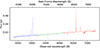 |
Fig. 1. NGC 3982 concatenated spectra observed with the LR-B, LR-V, and LR-R VPHs in blue, green, and red, respectively. Each spectrum was obtained by combining the 567 individual spectra measured simultaneously with the MEGARA LCB IFU. |
MEGARA VPH characteristics.
No reddening correction was applied to the emission-line fluxes, as our analysis relies on relative line ratios involving transitions close in wavelength (e.g. those used in the BPT and WHAN diagrams), which are essentially insensitive to extinction effects. This is a standard practice in emission-line diagnostics (Veilleux & Osterbrock 1987; Dopita et al. 2016) and has been used in recent high-redshift studies (Tripodi et al. 2024).
The MEGADES DR11 provides both the reduced observations and some analyses performed on the stellar component and the interstellar gas component of the galaxies in the sample. The process followed for the reduction of the observations is the standard MEGARA IFU data reduction procedure using the MEGARA data reduction pipeline v0.12.0 (Pascual et al. 2022), as described in the MEGARA Reduction Cookbook (Castillo-Morales et al. 2020)2 and in the sample presentation paper (Chamorro-Cazorla et al. 2023), where the DR1 was first introduced and whose preparation included the data reduction carried out by our team. In this study we made use of those publicly released reduced data products.
3. Analysis
3.1. Emission lines
To perform the analysis of the ionised gas present in the ISM of the galaxies in the MEGADES sample, we used the already reduced and processed data presented in Sect. 2. More specifically, among all the data products generated for the MEGADES DR1, we analysed the files containing the independent fit of each emission line (named [OBJECT]_[VPH]_[SPECTRAL_LINE].fits). These files contain the information of each emission line fitting obtained by applying Gauss-Hermite models. These emission-line fits are obtained by using the megaratool analyze_rss created for this purpose and for other MEGARA emission-line data. More detailed information on the analysis conducted on these spectral features can be found in Chamorro-Cazorla et al. (2023). In particular, the fluxes of the Balmer lines (Hβ and Hα) used throughout this work are corrected for the underlying stellar absorption. This correction was performed by fitting and subtracting the stellar continuum using a full spectral fitting approach, as described in detail in Chamorro-Cazorla et al. (2023). Therefore, the resulting emission line fluxes are free from contamination by the stellar population and suitable for diagnostic analysis.
The broad spectral coverage of the MEGADES observations provides us with information on the ionised gas based on different strong emission lines: Hβ and [O III]λ5007 lines, Hα, [N II]λ6584, and the two [S II] lines, [S II]λ6717 and [S II]λ6731. We detail the definition of the windows set for the emission-line fittings in Table 2.
Line fitting window definitions in the rest frame.
Before starting to analyse the ionised gas emission lines, we wanted to verify to what extent we can be confident in our results. To do so, we checked the limit of the S/N of our data at which our measurements become unreliable. The method used for this verification is based on comparing the measurements of the flux and the line-of-sight velocity dispersion (σ) of two different emission lines produced by the same ion, the same excitation mechanism and starting from the same upper level. For this purpose, we applied this technique to the emission line doublet [O III]λ4959 and [O III]λ5007. Figure 2 shows the relation between the flux (top panel) and the velocity dispersion (bottom panel) measured on both lines as a function of the S/N (per pixel) at the peak of the weakest line ([O III]λ4959) for measurements performed on all data included in the MEGADES survey.
As expected, Fig. 2 shows that the lower the S/N the greater the scatter on the ratio obtained when measuring the flux and velocity dispersion of each of these two lines. To get similar values for σ([O III]λ5007) and σ([O III]λ4959), we had to reach at least a S/N at the peak of the line of S/N > 10. This value is the threshold that we used throughout this work whenever we made use of ionised-gas data.
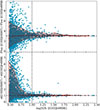 |
Fig. 2. Flux (top panel) and velocity dispersion (bottom panel) ratios of [O III]λ5007 to [O III]λ4959 as a function of the S/N of [O III]λ4959 measured on the peak of the line using all data included in the MEGADES survey. In both cases, the shaded region between the dashed red lines marks the position of the 10th and 90th percentiles. The solid red line indicates the median value of the flux or velocity dispersion ratio at each S/N value. |
Although Galactic extinction correction was not applied to our spectra, the impact of such a correction on our derived line ratios is negligible. Our calculations indicate that the relative extinction affecting the AHα/A[N II]λ6584 ratio is 1.004, while the AHβ/A[O III]λ5007 ratio is affected by a relative extinction of 1.039. The average extinction in the case of our sample of galaxies in the g-band is approximately 0.15 mag, which implies changes in the line ratios of −0.0001 dex for Hα/[N II]λ6584 and −0.0013 dex for Hβ/[O III]λ5007. Based on these results, we can conclude that the relevance of Galactic extinction in the context of nearby-line ratios is not significant.
3.2. Effective radii estimation
To establish comparisons in our estimates of metallicity gradients between the various galaxies in our sample, we estimated the effective radius. This measure allows us to better contextualise the metallicity variations in relation to the physical dimensions of the galaxies. For the estimation of the effective radii of the galaxies in the sample, available in Table A.1, we applied the method based on the asymptotic magnitude estimation described in Cairós et al. (2001) and applied in works such as Gil de Paz et al. (2007). Therefore, we used the brightness profiles of each of the galaxies calculated from their photometric decomposition elliptical isophotes (panel a in Fig. 3) to estimate the cumulative flux at each radius (panel b in Fig. 3) and how it changes as a function of the cumulative flux gradient (panel c in Fig. 3). If we perform a linear fit of the cumulative flux gradient as a function of its gradient, we can use the y-intercept of this fit as the asymptotic magnitude of the galaxy. Once we had this information, to calculate the effective radius of the galaxy we simply located the semi-major axis at which the cumulative flux is equal to the asymptotic magnitude plus 2.5log(2).
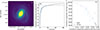 |
Fig. 3. Panel (a): Pan-STARRS g-band image of the galaxy NGC 0718, with the isophotes calculated using Photutils overplotted in white. Panel (b): Cumulative magnitude derived from the previously measured isophotes as a function of the semi-major axis. Blue dots correspond to the integrated magnitude within each isophote, and the dashed black line is a smoothed interpolation of the distribution. The horizontal solid blue line indicates the asymptotic magnitude of the galaxy, and the orange cross marks the semi-major axis at which the cumulative magnitude reaches a value equal to the asymptotic magnitude plus 2.5log(2), corresponding to the effective radius. Panel (c): Cumulative magnitude as a function of the cumulative magnitude gradient. Each blue dot corresponds to a given isophote. The dashed black line shows a linear fit to the data points at the lowest gradients, and the vertical dashed-dotted black line marks the zero gradient. The intercept of the linear fit with the vertical axis is used to estimate the asymptotic magnitude of the galaxy. |
The images we used to perform the photometric decomposition of the MEGADES galaxies come from the Pan-STARRS survey (Chambers et al. 2016). Specifically, we used the g-band cutout images of 250 ″ × 250 ″(1000 × 1000 pixels) in size available at the Pan-STARRS1 Database (Flewelling et al. 2020). It is worth remembering that the field of view of the MEGARA IFU is 12.5 × 11.3 arcsec2, so we can only cover the most central regions of the Pan-STARRS image (50 × 45 pixels).
The photometric analysis has been carried out using the Photutils (Bradley et al. 2023) software package included in Astropy, which is specifically designed to perform this kind of task. The isophote package within Photutils fits different elliptical isophotes to the input data and allows us to obtain a model of the data from these fits based on the iterative method created by Jedrzejewski (1987).
4. Results
4.1. Diagnostic diagrams
Since diagnostic diagrams were first proposed by Baldwin et al. (1981), comparing the flux ratios [O III]λ5007/Hβ versus [N II]λ6584/Hα, BPT diagrams have been very useful for discerning the excitation mechanisms responsible for the ionisation and line emission in the ISM. In the left panel of Fig. 4 we show the results obtained from measuring the aforementioned flux ratios in all the spaxels of the sample (when they meet the quality criteria explained in Sect. 3.1). Different panels in this figure show the evolution of the distribution of the points when plotting these diagrams using spaxels at different galactocentric distances. These cuts at different galactocentric distances (R < 0.25 kpc, 0.25 kpc < R < 0.5 kpc, 0.5 kpc < R < 1 kpc and R > 1 kpc) show that most of the spaxels with emission lines excited by the influence of the central AGN disappear beyond 0.25 kpc. This is not surprising since as we move away from the galactic centre, the influence of the AGN becomes gradually weaker at a rate that depends on the brightness of the AGN itself and the seeing of the observations. At all distances we have regions excited by photoionisation from massive stars and, as we get farther away from the innermost region, it becomes the only existing excitation mechanism. Note that, in principle, the ionisation by the AGN should only reach the broad-line region (BLR) and narrow-line region (NLR), both of which are much more compact that the MEGARA spaxel size for any of our objects. The fact that we find spaxels with AGN-like line ratios beyond the innermost bin in galactocentric distance might be due to contamination coming from extended point-spread function associated with the nuclear (point-like) AGN emission.
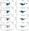 |
Fig. 4. Left panels: [O III]λ5007/Hβ versus [N II]λ6584/Hα BPT diagram of all spaxels in the MEGADES sample for galactocentric distance cuts of (from top to bottom): < 0.25 kpc, between 0.25 and 0.5 kpc, between 0.5 and 1 kpc, and > 1 kpc. The size of each point depends on the S/N measured at the peak of the [N II]λ6584 line. The dashed, dotted, dash-dotted, and solid lines represent the Kewley et al. (2001), Kauffmann et al. (2003), Stasińska et al. (2006), and Espinosa-Ponce et al. (2020) demarcation curves, respectively. Right panels: Relationship between [O III]λ5007/Hβ and the velocity dispersion measured on the Hβ line for the same galactocentric distances shown in the left panels. The size of each point depends on the S/N measured at the peak of the Hβ line. Grey dots in the backgrounds correspond to all points in the sample. |
In the right panels of Fig. 4 we show the velocity dispersion values measured on the Hβ lines (σHβ) and display them against [O III]λ5007/Hβ in order to compare these results with those of the BPT diagrams to their left, for the same cuts in galactocentric distances. As expected, the spaxels with lines showing the greatest velocity dispersion (σHβ > 100 km s−1) appear in the regions with R < 0.25 kpc, the innermost regions, although we find values corresponding to different ionisation mechanisms in this region. This is also related to the influence of the BLR of the AGN. Here we should note that no multi-component decomposition of the Balmer lines was attempted in these innermost regions of AGN-host galaxies, so the Hβ line widths reported are likely intermediate between those of the BLR and NLR, even if these fits were performed adopting a rather flexible Gauss-Hermite functional form. In this diagram we also report on the presence of a U-shape in the [O III]λ5007/Hβ ratio that is particularly noticeable at the innermost regions (R < 0.5 kpc) mainly because the contribution of spaxels with highσ but also high-[O III]λ5007/Hβ ratios. This deviates from the general trend of having spaxels with progressively lower [O III]λ5007/Hβ ratios as σ increases, until we reach the turning point at log(σHβ(km s−1)) ∼ 1.5. The most likely explanation for that trend is that, as σ is higher in regions less affected by the AGN, the contribution of shocks associated with sites of star formation (stellar winds and supernovae) increases; this leads to a larger contribution of these mechanisms to the line emission, and these mechanisms are known to lead to lower ionisation. This naturally boosts lower-ionisation species (and emission lines), such as [N II]λ6584 (see below), but dims higher-ionisation ones, such as [O III]λ5007.
The difference in the number of spaxels between the two panels of Fig. 4 arises because the left-hand panels combine lines observed with different gratings (LR-B for Hβ and [O III]λ5007, LR-R for Hα and [N II]λ6584). In this case only spaxels with information available in both gratings can be used. In addition, the S/N criterion is applied to different lines on each axis, which introduces further differences in the selected sample. Finally, the effective overlap of the IFU fields depends on how well the telescope pointings of the LR-B and LR-R observations are aligned. The pointings are not always perfectly accurate and in some cases the offset can be significant, as discussed in Chamorro-Cazorla et al. (2023). By contrast, the right-hand panels, based solely on LR-B data, is not affected by these limitations and therefore includes more spaxels. In Fig. 5, both axes rely on LR-R lines, so the same spaxels are present in the two panels.
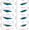 |
Fig. 5. Left panels: [N II]λ6584/Hα versus the equivalent width of the Hα line for different galactocentric distance cuts (from top to bottom): < 0.25 kpc, between 0.25 and 0.5 kpc, between 0.5 and 1 kpc, and > 1 kpc. The dashed line marks the boundary proposed by Stasińska et al. (2006) to distinguish between star-forming regions (labelled SF) and AGNs. The dotted line indicates the boundary established by Kewley et al. (2006) to separate, within the AGN area, Seyferts from LINERs (labelled L). The dash-dotted line separates the region populated by lines produced in RGs proposed by Cid Fernandes et al. (2011). Right panels: [N II]λ6584/Hα versus velocity dispersion of the Hα line for the same galactocentric distance cuts. In all panels, the size of each point depends on the S/N measured at the peak of the [N II]λ6584 line. Grey dots in the background correspond to all points in the sample. |
Another method used to establish the origin of emission lines is the so-called WHAN diagram (Cid Fernandes et al. 2010). This diagram represent [N II]λ6584/Hα versus the equivalent width of Hα (EWHα) and enable us to distinguish regions excited by star formation from those excited by AGN, differentiating Seyfert from LINER zones (or LINER-like zones; see below). The innovative aspect of this classification is the inclusion of regions that have classically been considered low-luminosity AGNs (and, in particular, LINERs) but are better described as presenting LINER-like excitation conditions. According to these authors, this new mechanism occurs in ‘retired galaxies’ (RGs), which are galaxies that have stopped forming stars and whose source of ionisation comes from HOLMESs (Binette et al. 1994; see also the discussions by Singh et al. 2013; Papaderos et al. 2013, and Belfiore et al. 2016 on a similar type of objects, the low-ionisation emission-line regions). It should be noted that studies carried out by Byler et al. (2019) show that the EWHα produced by a population whose ionisation radiation is dominated by post-asymptotic giant branch stars typically varies between 0.1 Å and 2.5 Å, especially at ages over log10(t/yr) ≳ 9.
An important feature of the WHAN diagram is its use of a simple constant threshold in log([N II]λ6584/Hα) to separate star-forming and AGN-like regions. This threshold, typically set at log([N II]λ6584/Hα) = − 0.4 originates from the work of Stasińska et al. (2006), who showed that this ratio alone can effectively classify galaxies into normal star-forming (log([N II]λ6584/Hα) ≤ −0.4), hybrid (−0.4 < log([N II]λ6584/Hα) ≤ −0.2), and AGN-dominated (log([N II]λ6584/Hα) > −0.2) categories. Thus, the WHAN diagram inherits this empirical demarcation, making it particularly useful when other diagnostic lines are unavailable or suffer from low S/N.
We show the WHAN diagram using the observations of the MEGADES sample in Fig. 5 (left panels). We find that the distribution of points in our sample is similar to the one obtained by (Cid Fernandes et al. 2011) using SDSS (Sloan Digital Sky Survey) data (see their Fig. 6). According to this diagram, part of the emitting regions we detect (those with EWHα < 3 Å) come from ionisation by HOLMES. This mechanism is present at practically all galactocentric distances. Although the WHAN and BPT diagrams share a similar criterion in terms of log([N II]λ6584/Hα), the inclusion of EWHα in WHAN leads to differences in the classification of individual spaxels. In particular, we find that ∼95% of the regions identified as AGNs in the BPT diagram using the Stasińska et al. (2006) criterion are also classified as AGNs in the WHAN diagram, highlighting both the consistency and the added diagnostic value of this diagram.
In the right panel of Fig. 5 we present the measurements obtained for [N II]λ6584/Hα ratio versus the Hα velocity dispersion. In this case we observe a clear correlation with larger values of [N II]λ6584/Hα ratio showing larger Hα velocity dispersion. According to the scenario proposed above to explain the U-shape in the [O III]λ5007/Hβ versus σ diagram, this trend could be explain as due to the enhanced contribution of shock-excitation to the emission from low-ionisation species such as [N II]λ6584 at progressively larger σ values.
The fact that the measurement of the ionised-gas velocity dispersion allowed us to identify spaxels affected by (broad) AGN emission, have led us to evaluate the BPT diagrams of our emission-line regions in the MEGADES galaxies as a function of this parameter. Thus, in Fig. 6 we show again the classical BPT diagrams of [O III]λ5007/Hβ versus [N II]λ6584/Hα (left panels) and [O III]λ5007/Hβ versus ([S II]λ6717+[S II]λ6731)/Hα (right panels) but now split in different ranges of σHα, namely σHα < 30 km s−1 (top panels), 30 km s−1 < σHα < 70 km s−1 (middle panels) and σHα > 70 km s−1 (bottom panels).
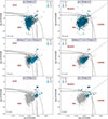 |
Fig. 6. BPT diagrams of [O III]λ5007/Hβ versus [N II]λ6584/Hα (left panel) and [O III]λ5007/Hβ versus ([S II]λ6717+[S II]λ6731)/Hα (right panel). Both panels show the diagrams for three different cuts as a function of the velocity dispersion measured on the Hα line (from top to bottom): < 30 km s−1, between 30 and 70 km s−1, and > 70 km s−1. In the left panel, the dashed, dotted, dash-dotted, and solid lines represent the Kewley et al. (2001), Kauffmann et al. (2003), Stasińska et al. (2006), and Espinosa-Ponce et al. (2020) demarcation curves, respectively. In the right panel, the dashed, dotted, and solid lines represent the Kewley et al. (2001, 2006), and Espinosa-Ponce et al. (2020) demarcation curves, respectively. The size of the points in the left and right panels depends on the S/N measured at the peak of the [N II]λ6584 line and [S II]λ6717, respectively. Grey dots in the backgrounds correspond to all points in the sample. |
Both diagrams show that for lower velocity dispersions (σHα < 30 km s−1) the spaxels are mostly located where the excitation is due to photoionisation by massive stars. For intermediate σHα values (30 km s−1 < σHα < 70 km s−1) we still have a majority of photoionisation-dominated line ratios but they occupy regions closer to the AGN dividing line. Finally, for the highest velocity dispersion values (σHα > 70 km s−1) we find that all spaxels are located in the AGN excitation region for the [N II]λ6584/Hα diagram and in the case of the [S II]λ6717+S II]λ6731 diagram most of them are also located in this region, although this depends on the specific demarcation considered.
The identification of relations between the velocity dispersion of the ionised gas emission lines and the mechanisms driving their excitation is a predictable finding, supported by previous research, as evidenced by the work of D’Agostino et al. (2019). They establish a relation between the velocity dispersion and the way in which the regions of a galaxy are distributed in the BPT diagram (emission line ratio information) in order to define a criterion that enables the determination of the predominant excitation mechanism in each area of the galaxy. However, this criterion is based on a data-dependent method, as the authors themselves mention in the paper, and since they only analyse one galaxy (NGC 1068), we considered it unsuitable to apply it to our sample data. The fact that we included data from 43 different galaxies, each of them with different metallicities and with different spatial resolutions due to their different distances, means that our data may introduce a large scatter in the BPT diagram of the sample, especially along the boundary that divides the excitation mechanisms.
The potential to identify the mechanisms responsible for the excitation of the different components of interstellar gas by measuring their velocity dispersion highlights the need for instruments with high spectral (and spatial) resolution in order to have sufficient resolving power to be able to measure the lines with the lowest velocity dispersion. This study has only been possible thanks to the unique combination of high spatial and spectral resolution of the observations collected with MEGARA.
4.2. Dynamical selection of excitation mechanisms
Due to the fact that the behaviour of the different spaxel-by-spaxel line ratios as a function of line width can be interpreted in terms of the relative contribution of AGNs, shocks, and H II regions photoionisation within each spaxel, we attempted to provide a diagnosis based exclusively on dynamical properties. We first assumed that in many cases more than one mechanism might be at play but that different lines have a different degree of sensitivity to those mechanisms. Thus, while the [N II] lines are very sensitive to low-velocity shocks, narrow Balmer lines are sensitive to all mechanisms (including the NLR of AGNs at intermediate line widths) and very broad Balmer lines are almost exclusively produced in the BLR of AGNs. Therefore, there where different mechanisms at play, the comparison between the line widths of these lines (besides the impact on line ratios described in the previous section) could provide further information, and additional diagnostics, on the nature of the dominant excitation mechanism.
In the left panel of Fig. 7 we have plotted the velocity dispersion measured in the [N II]λ6584 and Hα lines against the velocity dispersion in the Hα line. By doing so, we tried to establish a purely dynamical criterion to distinguish the excitation mechanisms that have led to the appearance of these emission lines.
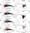 |
Fig. 7. Left panels: Relationship between the measured ratio of velocity dispersions of [N II]λ6584 and Hα lines versus the velocity dispersion on the Hα line for different galactocentric distance cuts. The dashed, dash-dotted, and solid black curves represent lines with a constant broadening with respect to the Hα line of 30, 50, and 70 km s−1, respectively. The dashed orange lines indicate the boundaries between the regions defined by the dynamic selection of excitation mechanisms explained in this section. Right panels: BPT diagram of [O III]λ5007/Hβ versus [N II]λ6584/Hα corresponding to the points falling within each of the regions defined in the left panel. From top to bottom we have the BPT diagram for the lines excited by shocks-like mechanism, photoionisation, and AGNs. The dashed, dotted, dash-dotted, and solid lines represent the Kewley et al. (2001), Kauffmann et al. (2003), Stasińska et al. (2006), and Espinosa-Ponce et al. (2020) demarcation curves, respectively. In both panels blue dots denote lines measured in galaxies classified as Seyfert or LINER (see Table A.1), while the red dots represents the rest of the galaxies. The size of the points depends on the S/N measured at the peak of the [N II]λ6584 line. Grey dots in the backgrounds correspond to all points in the sample. |
The boundaries separating the regions populated by lines excited by (or dominated by) different excitation mechanisms have been selected on the basis of the following criteria. First, the line separating the AGN region from the shock and photoionisation regions has been adopted according to the full width at half maximum lower limit of 200 km s−1 given in Vaona et al. (2012) for lines belonging to the NLR. This, translated into velocity dispersion, implies a σ ∼ 85 km s−1. To add some conservative margin to this limit, we used σHα = 100 km s−1 as the division between the zone of excitation produced by AGNs and the rest of the mechanisms.
For σHα < 100 km s−1, we applied two different criteria. First, for low σHα values, we made a cut at constant σ[N II]λ6584/σHα − 1. This constant value represents regions that would show a [N II]λ6584 line broader than Hα by a constant fraction of the line width of Hα. Then, for σHα > 30 km s−1 we applied a constant (quadratic) broadening in velocity of Δ = 30 km s−1. In Fig. 7 we show the predictions in σ[N II]λ6584/σHα − 1 for such 30 km s−1 broadening but also for 50 and 70 km s−1. These lines correspond to the following equation:
![Mathematical equation: $$ \begin{aligned} \frac{\sigma _{[\mathrm{N}\,ii ]\lambda 6584}}{\sigma _{\mathrm{H}\alpha }} = \sqrt{1 + \left( \frac{\Delta }{\sigma _{\mathrm{H}\alpha }} \right) ^2}. \end{aligned} $$](/articles/aa/full_html/2026/01/aa56147-25/aa56147-25-eq7.gif) (1)
(1)
To verify that the proposed cutoffs do a good job of isolating the different excitation mechanisms, we split the different spaxels by galactocentric distance and included information on the nature of the objects in our sample regarding the nuclear activity as published in the literature. Thus, we plot in blue those spaxels (independently of their galactocentric distance) coming from galaxies that have been identified in the literature as LINER or Seyfert (see Table A.1; taken from the NASA/IPAC Extragalactic Database), and in red spaxels from galaxies spectroscopically classified as H II galaxies, starburst, or star-forming galaxies in general. Given that our observations target the central ∼0.5–3 kpc of our galaxies, when nuclear activity is present, it should play a major role on the ionising properties of our spectra. As such, the Seyfert/LINER classification from the literature already provides a reasonable proxy for assessing whether AGN-related processes dominate the excitation mechanisms in the corresponding spaxels. In summary, the proposed dynamical criterion adopts (from high to low velocity dispersion): (1) a minimum σHα of 100 km s−1 for AGN-dominated (NLR or BLR) spaxels, (2) a (limiting) broadening of Δ = 30 km s−1 for spaxels with Hα line widths below 100 km s−1 but above 30 km s−1, to separate between the spaxels ionised by shocks and UV photons, and (3) a linear offset in σ[N II]λ6584 − σHα that is proportional to σHα in the case of the spaxels with the narrowest lines, i.e. σHα < 30 km s−1.
Applying the criteria described above, we obtain a distribution of points in the BPT diagram as shown in the right-hand panels of Fig. 7. We can see that the dynamic distinction we made separates the different zones quite well from each other. In the left-hand panels, galaxies classified as Seyfert or LINER are distributed within the BPT diagram either in the regions of AGN-excited lines or in the intermediate zones between that region and the emission region of the HII regions. We note that the non-nuclear regions of AGN-host galaxies are expected to have line ratios (and velocity dispersion values) compatible with being ionised by massive stars (see the middle panel).
4.3. Ionised-gas metallicity gradients
The metallicity of ionised-gas can be estimated from several strong–line indicators including the [N II]λ6584/Hα ratio (also called the N2 indicator; see Marino et al. 2013 and references therein). These authors established a relation between the oxygen abundance derived from electron temperature-sensitive lines (namely [O III]λ4363 and [N II]λ5755) and the value of [N II]λ6584/Hα in the ISM of galaxies using measurements mainly from the literature but also from the CALIFA survey. Using this relation we can easily convert our N2 measurements into measurements of the oxygen abundance in the ionised-gas and, therefore, of the overall gas metallicity. However, this relation is only valid when the excitation mechanism that has given rise to the line emission is photoionisation, since the data used for its calibration come from photoionised HII regions in very nearby galaxies, so before calculating abundances it is necessary to discriminate the origin of the lines we are studying. It is also important to note that this calibration carries an intrinsic scatter of about 0.16 dex (Marino et al. 2013), mostly driven by galaxy-to-galaxy variations in the reference sample. Within a given galaxy, spaxels from the same observation are correlated, so this scatter acts essentially as an upper bound on the uncertainty and in practice it affects the absolute zero-point of the gradients more strongly than their relative slopes.
Based on the studies we describe in the previous section (see Fig. 7), we are able to identify the main mechanism that has produced the line emission of the spaxels in our galaxies and therefore derive proper metal abundance in the ionised-gas phase. We can also compare the results obtained when measuring metallicities using all the [N II]λ6584 line ratios available in the sample with those estimated using spaxels whose line emission is produced by photoionisation exclusively. In this section we focus on the radial variation of the metal abundance, including the determination of metallicity gradients, since azimuthal variations are beyond the scope of this paper. Thus, in Fig. 8 we first show the results of the best-fitting oxygen abundance gradients obtained for the galaxy NGC 3982 from our N2 measurements calculated in the two ways, including and excluding line ratios that could be arising from spaxels ionised by mechanisms other than photoionisation. These gradients were calculated by dividing the range of galactocentric distances covered in each observation into ten equal intervals and calculating the median value of the points belonging to each interval. The best fits for all the galaxies in the sample are shown in Appendix B and the results can be found in Table A.1. Hereafter, every time we discuss about photoionised-only spaxels we will be referring those spaxels selected to have their line emission due to UV photons, according to the dynamical criteria defined in Fig. 7.
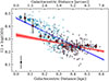 |
Fig. 8. Oxygen abundance (i.e. 12 + log(O/H)) estimations based in the calibration by Marino et al. (2013) as a function of galactocentric distance for the galaxy NGC 3982. Gradients have been derived using the median values estimated for different galactocentric distance intervals. Within each galactocentric distance interval, the median values of the data are represented by blue or red squares. The blue (red) dots represent metallicity measurements obtained from all the spaxels (spaxels whose emission lines originated in star-forming regions; see text). The blue and red bands indicate the results of our Bayesian linear best fits to the data with the same colour coding as for the individual measurements. The dark and light shaded bands correspond to the confidence intervals at 1σ and 2σ levels, respectively. The black dot at the bottom left represents the median error of all the blue points. |
The resulting best-fitting ionised-gas metallicity gradients and central extrapolated metallicities are shown in Fig. 9. This figure also includes information on the kinematic class of the objects analysed. These kinematic classes have been determined based on the work by van de Sande et al. (2017) and, although these results are already available, the full analyses of our application of these criteria to the MEGADES sample data will be published in a forthcoming publication (Chamorro-Cazorla et al., in prep.). To understand this kinematic classification in a simple way, we note that objects classified in classes 1 and 2 are considered slow rotators and objects between classes 3 and 5 are considered fast rotators.
Figure 9 shows that the central abundances of the galaxies in the sample vary between 8 and 8.7 dex in the 12+log(O/H) scale (for comparison, the oxygen abundance in the solar photosphere is 8.69 ± 0.05; Asplund et al. 2009). On the other hand, we see that most of the galaxies show very low or almost null metallicity gradients, especially if we look at the fast rotators with central metallicities below 8.37 dex, with a median value for these gradients of 0.005 dex R and a dispersion of 0.422 dex R
 . Above that value, fast rotators show slightly negative metallicity gradients with some degree of correlation between slope and y-intercept with a median value for the slope of −0.681 dex R
 and a dispersion of 0.933 dex R
 . The median value estimated for all the galaxies included in MEGADES is −0.025 dex R
 with a dispersion of 0.766 dex R
 . To place our results in context, previous work measuring the oxygen abundance in nearby galaxies shows results like those of Sánchez-Menguiano et al. (2016), with median values of the slopes measured in galaxies belonging to the CALIFA sample of −0.07 dex R
 dex R
dex R using the same calibration proposed by Marino et al. (2013) used in this work. It is worth noting here that the data included in the CALIFA sample have observations covering a field of view of 1 arcmin2 while ours stay in much more inner regions of galaxies, as well as having observations of 939 galaxies. We note here that although we show only the marginalised errors in both quantities, these two quantities are correlated for each individual fit in the same direction (Chamorro-Cazorla et al. 2022). However, the wide range in properties (0.7 dex in the case of the central metallicity), much larger than the individual errors, indicate that the correlation found is not only driven by the covariance between the two parameters of each individual fit. Besides, this relatively tight correlation is only found in fast rotators, with slow rotators showing a much larger dispersion in metallicity gradient for a given central metallicity. For the majority of slow rotators the gradients are more pronounced (more negative) than those of the fast-rotators of the same central metallicity, although their most notorious difference is their significantly larger dispersion across this plot.
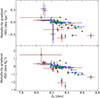 |
Fig. 9. Metallicity gradients of the ionised gas measured for all galaxies in our sample. The orange circles indicate galaxies that were classified as slow rotators (dynamical classes 1 and 2) and cyan squares indicate fast rotators (classes 3 through 5). Top panel: Gradients computed as a function of galactocentric distance (in kpc). Bottom panel: Gradients computed as a function of the effective radius. The x-axis indicates the y-intercept of the linear fit to the metallicity gradient. Each galaxy is represented twice as we include the results of the best fits obtained using both photoionised spaxels (points with red error bars) and all spaxels (points with blue error bars). |
We also see that the error bars for the fits obtained from photoionised-only spaxels are larger than for those obtained using all data, mainly because the former have fewer points to fit and, in many cases, their range of distances for the calculation is significantly reduced. In general, the radial gradients derived correspond to regions that are at galactocentric distances below 2 kpc (see the individual fits in Appendix B).
To show the difference in the best-fitting parameters obtained with the different datasets (photoionised-only and all spaxels), we present them in Fig. 10, colour-coded by their kinematical state. The corresponding frequency distributions for the entire sample are shown along with their medians (marked as dashed lines). We find a long tail of fast rotators towards more positive metallicity gradients and lower central metallicities when computed using photoionised-only spaxels. This tail can create the impression of a correlation between slope and intercept for the fast rotators (cyan squares in Fig. 10). This trend could be mostly driven by the natural degeneracy between the two parameters, since steeper negative slopes are typically associated with higher intercepts, which makes the points distribute along this axis. The effect is accentuated by two outliers with particularly large uncertainties, and once these are excluded the correlation becomes much less evident. Whereas in Fig. 9 the broader dynamic range of the data dominates over such degeneracies, the restricted range in Fig. 10 enhances this impression. Confirming whether a genuine correlation exists would require additional data to improve the statistics.
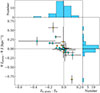 |
Fig. 10. Ionised-gas metallicity gradients computed when photoionised-only spaxels are used versus when all spaxels are used. The difference between y-intercepts is shown on the x-axis, while the difference between slopes is included on the y-axis. Orange circles (cyan squares) represent the results of the fits to our slow (fast) rotators. The dashed lines in the central plot mark the zero position on each axis. The thick dashed lines in the frequency histograms mark the median value of the data on each axis. |
At the same time, when considering the full distribution, the median values of these differences remain very close to zero (−0.003 in the case of abundance and −0.001 in the case of gradient). Thus, the median values of these differences are practically null in both cases.
5. Discussion
In this section we analyse how these results provide some clues as to the relative role of the different mechanisms involved in the evolution of galaxies and, in particular, in shaping their current-day spectrophotometric, chemical, and dynamical properties.
Concerning the diagnosis of ionised gas, the different analyses performed by exploiting BPT diagrams of [O III]λ5007/Hβ versus [N II]λ6584/Hα and [S II]λ6717+[S II]λ6731, together with the study of their radial variations and their relationships with the velocity dispersion of the emission lines that populate them, led us to attempt to differentiate the predominant excitation mechanisms in each spaxel on the basis of a purely dynamical criterion. This criterion, based on the values of the [N II]λ6584 and Hα velocity dispersion and the relation between them, has proved to be quite effective. This criterion, given the importance of properly distinguishing the dominant mechanisms responsible for the ionised gas emission, can save a lot of telescope time in cases where it is not possible to simultaneously observe the spectral ranges [O III]λ5007/Hβ and [N II]λ6584/Hα, as is the case for MEGARA.
Our diagnoses have shown that a large number of spaxels (at any galactocentric distance) have emission-line ratios that indicate the presence of shocks based on both their line ratios (typically high [N II]λ6584/Hα and intermediate [O III]λ5007/Hβ) and their widths (intermediate between photoionisation by massive stars and AGNs, either in the NLR or BLR). In this context, excitation with shocks is naturally associated with the onset of galactic winds. Given the relatively high masses of these objects, these winds would not imply the loss of gas mass, probably not even the escape of chemically enriched outflows into the intergalactic medium, but can certainly produce the redistribution of metals on several-kiloparsec scales (see Christensen et al. 2018). Under this scenario, when a galactic wind is in place, some of the gas is blown into the circumgalactic environment; eventually it falls back into the plane of the galaxy, though not necessarily at the same radii at which the wind was generated. In the case of a nuclear starburst that throws material into the circumgalactic medium that ends up falling into the outer parts of the disc, this material enriches the outer parts and causes the metallicity gradients to flatten (dilute). Another piece of evidence of the presence of galactic winds (neutral in this case) in some of our galaxies is the finding of NaI D absorption with complex kinematics and large equivalent widths (Chamorro-Cazorla et al. 2023). Another mechanism that can produce widespread shocked-like line ratios is the presence of large-scale shocks induced by bars (see e.g. Maciejewski et al. 2002). Note that in these cases, where the gravitational potential has a non-axisymmetric component, we would also expect a flattening in the physical properties of the galaxies (age and metallicity) with galactocentric distance compared to those expected from the perspective of a purely inside-out galaxy formation scenario, at least for a range of galaxy masses (see Zurita et al. 2021, and references therein).
The availability of a dynamical criterion for selecting regions whose line emission arises from photoionisation from massive stars prevents the bias in the ionised-gas metallicity measurements that a selection based purely on line ratios would introduce. Furthermore, the impact of the spaxels dominated by other mechanisms is small, since there is little difference in the ionised-gas metallicity gradients derived with the two datasets (photoionised-only and all spaxels). Besides, given our limited range in galactocentric distance, we expect that such a potential bias would be even less of a problem in works covering the (outer) discs, where emission due to AGNs or shocks (or even from ‘retired’ stellar populations) should be minimal. The correlation found (especially in fast rotators) between central abundances and gradients – gradients becoming increasingly negative as central abundances increase – supports the idea of inside-out formation and the presence of diffusion mechanisms in the sample galaxies (i.e. the redistribution of metals by galactic winds, gas radial transfer by bars, and the contribution of minor mergers). Under this scenario, a metallicity distribution with a certain gradient and central abundance would evolve through radial displacements of gas flattening the gradients and reducing the central abundances. The fact that we find a similar trend in the stellar metallicities indicates that this is not simply due to the gas having been diluted recently with externally accreted pristine gas.
Username: ‘public’, password: ‘6BRLukU55E’.
Acknowledgments
We/IPARCOS acknowledge/s the support from the “Tecnologías avanzadas para la exploración de universo y sus componentes” (PR47/21 TAU) project funded by Comunidad de Madrid, by the Recovery, Transformation and Resilience Plan from the Spanish State, and by NextGenerationEU from the European Union through the Recovery and Resilience Facility. The authors acknowledge the support of AC3, a project funded by the European Union’s Horizon Europe Research and Innovation programme under grant agreement No 101093129. MCC, AGdP, ACM, JG, CCT, JZ, NC and SP acknowledge financial support from the Spanish Ministerio de Ciencia, Innovación y Universidades (MCIU) under the grant RTI2018-096188-B-I00, PID2021-123417OB-I00 and PID2022-138621NB-I00. This research has made use of the NASA/IPAC Extragalactic Database, which is funded by the National Aeronautics and Space Administration and operated by the California Institute of Technology. The Pan-STARRS1 Surveys (PS1) and the PS1 public science archive have been made possible through contributions by the Institute for Astronomy, the University of Hawaii, the Pan-STARRS Project Office, the Max-Planck Society and its participating institutes, the Max Planck Institute for Astronomy, Heidelberg and the Max Planck Institute for Extraterrestrial Physics, Garching, The Johns Hopkins University, Durham University, the University of Edinburgh, the Queen’s University Belfast, the Harvard-Smithsonian Center for Astrophysics, the Las Cumbres Observatory Global Telescope Network Incorporated, the National Central University of Taiwan, the Space Telescope Science Institute, the National Aeronautics and Space Administration under Grant No. NNX08AR22G issued through the Planetary Science Division of the NASA Science Mission Directorate, the National Science Foundation Grant No. AST-1238877, the University of Maryland, Eotvos Lorand University (ELTE), the Los Alamos National Laboratory, and the Gordon and Betty Moore Foundation.
References
- Asplund, M., Grevesse, N., Sauval, A. J., & Scott, P. 2009, ARA&A, 47, 481 [NASA ADS] [CrossRef] [Google Scholar]
- Baldwin, J. A., Phillips, M. M., & Terlevich, R. 1981, PASP, 93, 5 [Google Scholar]
- Belfiore, F., Maiolino, R., Maraston, C., et al. 2016, MNRAS, 461, 3111 [Google Scholar]
- Belfiore, F., Maiolino, R., Tremonti, C., et al. 2017, MNRAS, 469, 151 [Google Scholar]
- Binette, L., Magris, C. G., Stasińska, G., & Bruzual, A. G. 1994, A&A, 292, 13 [NASA ADS] [Google Scholar]
- Bradley, L., Sipőcz, B., Robitaille, T., et al. 2023, https://doi.org/10.5281/zenodo.7946442 [Google Scholar]
- Bundy, K., Bershady, M. A., Law, D. R., et al. 2015, ApJ, 798, 7 [Google Scholar]
- Byler, N., Dalcanton, J. J., Conroy, C., et al. 2019, AJ, 158, 2 [Google Scholar]
- Cairós, L. M., Caon, N., Vílchez, J. M., González-Pérez, J. N., & Muñoz-Tuñón, C. 2001, ApJS, 136, 393 [CrossRef] [Google Scholar]
- Camps-Fariña, A., Raga, A. C., & Noriega-Crespo, A. 2018, A&A, 619, A11 [NASA ADS] [CrossRef] [EDP Sciences] [Google Scholar]
- Camps-Fariña, A., Beckman, J. E., Font, J., et al. 2020, MNRAS, 493, 1434 [Google Scholar]
- Carrasco, E., Gil de Paz, A., Gallego, J., et al. 2018, SPIE Conf. Ser., 10702, 1070216 [NASA ADS] [Google Scholar]
- Castillo-Morales, Á., Pascual, S., & Gil de Paz, A. 2020, https://doi.org/10.5281/zenodo.3932063 [Google Scholar]
- Cazzoli, S., Hermosa Muñoz, L., Márquez, I., et al. 2022, A&A, 664, A135 [NASA ADS] [CrossRef] [EDP Sciences] [Google Scholar]
- Chambers, K. C., Magnier, E. A., Metcalfe, N., et al. 2016, arXiv e-prints [arXiv:1612.05560] [Google Scholar]
- Chamorro-Cazorla, M., Gil de Paz, A., Castillo-Morales, A., et al. 2022, A&A, 657, A95 [NASA ADS] [CrossRef] [EDP Sciences] [Google Scholar]
- Chamorro-Cazorla, M., Gil de Paz, A., Castillo-Morales, Á., et al. 2023, A&A, 670, A117 [NASA ADS] [CrossRef] [EDP Sciences] [Google Scholar]
- Christensen, C. R., Davé, R., Brooks, A., Quinn, T., & Shen, S. 2018, ApJ, 867, 142 [CrossRef] [Google Scholar]
- Cid Fernandes, R., Stasińska, G., Schlickmann, M. S., et al. 2010, MNRAS, 403, 1036 [Google Scholar]
- Cid Fernandes, R., Stasińska, G., Mateus, A., & Vale Asari, N. 2011, MNRAS, 413, 1687 [Google Scholar]
- Cresci, G., Mannucci, F., Maiolino, R., et al. 2010, Nature, 467, 811 [Google Scholar]
- Croom, S. M., Lawrence, J. S., Bland-Hawthorn, J., et al. 2012, MNRAS, 421, 872 [NASA ADS] [Google Scholar]
- Curti, M., Cresci, G., Mannucci, F., et al. 2017, MNRAS, 465, 1384 [Google Scholar]
- D’Agostino, J. J., Kewley, L. J., Groves, B. A., et al. 2019, MNRAS, 485, L38 [CrossRef] [Google Scholar]
- Di Matteo, P., Pipino, A., Lehnert, M. D., Combes, F., & Semelin, B. 2009, A&A, 499, 427 [NASA ADS] [CrossRef] [EDP Sciences] [Google Scholar]
- Dopita, M. A., Kewley, L. J., Sutherland, R. S., & Nicholls, D. C. 2016, Ap&SS, 361, 61 [NASA ADS] [CrossRef] [Google Scholar]
- Espinosa-Ponce, C., Sánchez, S. F., Morisset, C., et al. 2020, MNRAS, 494, 1622 [Google Scholar]
- Ferland, G. J., Korista, K. T., Verner, D. A., et al. 1998, PASP, 110, 761 [Google Scholar]
- Flewelling, H. A., Magnier, E. A., Chambers, K. C., et al. 2020, ApJS, 251, 7 [NASA ADS] [CrossRef] [Google Scholar]
- Gil de Paz, A., Boissier, S., Madore, B. F., et al. 2007, ApJS, 173, 185 [Google Scholar]
- Gil de Paz, A., Carrasco, E., Gallego, J., et al. 2018, SPIE Conf. Ser., 10702, 1070217 [NASA ADS] [Google Scholar]
- Heckman, T. M., Armus, L., & Miley, G. K. 1990, ApJS, 74, 833 [Google Scholar]
- Ho, L. C. 2008, ARA&A, 46, 475 [Google Scholar]
- Ho, I. T., Kewley, L. J., Dopita, M. A., et al. 2014, MNRAS, 444, 3894 [Google Scholar]
- Jedrzejewski, R. I. 1987, MNRAS, 226, 747 [Google Scholar]
- Kauffmann, G., Heckman, T. M., Tremonti, C., et al. 2003, MNRAS, 346, 1055 [Google Scholar]
- Kewley, L. J., & Dopita, M. A. 2002, ApJS, 142, 35 [Google Scholar]
- Kewley, L. J., Dopita, M. A., Sutherland, R. S., Heisler, C. A., & Trevena, J. 2001, ApJ, 556, 121 [Google Scholar]
- Kewley, L. J., Groves, B., Kauffmann, G., & Heckman, T. 2006, MNRAS, 372, 961 [Google Scholar]
- Kewley, L. J., Nicholls, D. C., & Sutherland, R. S. 2019, ARA&A, 57, 511 [Google Scholar]
- López-Cobá, C., Sánchez, S. F., Bland-Hawthorn, J., et al. 2019, MNRAS, 482, 4032 [Google Scholar]
- Luridiana, V., Morisset, C., & Shaw, R. A. 2015, A&A, 573, A42 [NASA ADS] [CrossRef] [EDP Sciences] [Google Scholar]
- Maciejewski, W., Teuben, P. J., Sparke, L. S., & Stone, J. M. 2002, MNRAS, 329, 502 [NASA ADS] [CrossRef] [Google Scholar]
- Maiolino, R., & Mannucci, F. 2019, A&ARv, 27, 3 [Google Scholar]
- Marino, R. A., Rosales-Ortega, F. F., Sánchez, S. F., et al. 2013, A&A, 559, A114 [NASA ADS] [CrossRef] [EDP Sciences] [Google Scholar]
- Mingozzi, M., Cresci, G., Venturi, G., et al. 2019, A&A, 622, A146 [NASA ADS] [CrossRef] [EDP Sciences] [Google Scholar]
- Oliveira, C. B., Dors, O., Zinchenko, I., et al. 2024, PASA, 41, e099 [Google Scholar]
- Papaderos, P., Gomes, J. M., Vílchez, J. M., et al. 2013, A&A, 555, L1 [NASA ADS] [CrossRef] [EDP Sciences] [Google Scholar]
- Pascual, S., Picazo, P., Cardiel, N., Castillo-Morales, A., & Gil de Paz, A. 2022, https://doi.org/10.5281/zenodo.6043992 [Google Scholar]
- Pérez-Díaz, B., Masegosa, J., Márquez, I., & Pérez-Montero, E. 2021, MNRAS, 505, 4289 [CrossRef] [Google Scholar]
- Pérez-Montero, E. 2014, MNRAS, 441, 2663 [CrossRef] [Google Scholar]
- Pilyugin, L. S., & Grebel, E. K. 2016, MNRAS, 457, 3678 [NASA ADS] [CrossRef] [Google Scholar]
- Rich, J. A., Dopita, M. A., Kewley, L. J., & Rupke, D. S. N. 2010, ApJ, 721, 505 [NASA ADS] [CrossRef] [Google Scholar]
- Rich, J. A., Kewley, L. J., & Dopita, M. A. 2011, ApJ, 734, 87 [NASA ADS] [CrossRef] [Google Scholar]
- Rich, J. A., Torrey, P., Kewley, L. J., Dopita, M. A., & Rupke, D. S. N. 2012, ApJ, 753, 5 [NASA ADS] [CrossRef] [Google Scholar]
- Sánchez, S. F., Kennicutt, R. C., Gil de Paz, A., et al. 2012, A&A, 538, A8 [Google Scholar]
- Sánchez, S. F., Rosales-Ortega, F. F., Iglesias-Páramo, J., et al. 2014, A&A, 563, A49 [CrossRef] [EDP Sciences] [Google Scholar]
- Sánchez, S. F., Barrera-Ballesteros, J. K., Lacerda, E., et al. 2022, ApJS, 262, 36 [CrossRef] [Google Scholar]
- Sánchez-Menguiano, L., Sánchez, S. F., Pérez, I., et al. 2016, A&A, 587, A70 [NASA ADS] [CrossRef] [EDP Sciences] [Google Scholar]
- Schönrich, R., & Binney, J. 2009, MNRAS, 396, 203 [Google Scholar]
- Sellwood, J. A., & Binney, J. J. 2002, MNRAS, 336, 785 [Google Scholar]
- Sharda, P., Krumholz, M. R., Wisnioski, E., et al. 2021, MNRAS, 502, 5935 [NASA ADS] [CrossRef] [Google Scholar]
- Singh, R., van de Ven, G., Jahnke, K., et al. 2013, A&A, 558, A43 [NASA ADS] [CrossRef] [EDP Sciences] [Google Scholar]
- Stasińska, G., Cid Fernandes, R., Mateus, A., Sodré, L., & Asari, N. V. 2006, MNRAS, 371, 972 [Google Scholar]
- Sutherland, R., Dopita, M., Binette, L., & Groves, B. 2018, Astrophysics Source Code Library [record ascl:1807.005] [Google Scholar]
- Tripodi, R., D’Eugenio, F., Maiolino, R., et al. 2024, A&A, 692, A184 [NASA ADS] [CrossRef] [EDP Sciences] [Google Scholar]
- van de Sande, J., Bland-Hawthorn, J., Fogarty, L. M. R., et al. 2017, ApJ, 835, 104 [Google Scholar]
- Vaona, L., Ciroi, S., Di Mille, F., et al. 2012, MNRAS, 427, 1266 [NASA ADS] [CrossRef] [Google Scholar]
- Veilleux, S., & Osterbrock, D. E. 1987, ApJS, 63, 295 [Google Scholar]
- Veilleux, S., Shopbell, P. L., & Miller, S. T. 2001, AJ, 121, 198 [NASA ADS] [CrossRef] [Google Scholar]
- Vila-Costas, M. B., & Edmunds, M. G. 1992, MNRAS, 259, 121 [NASA ADS] [CrossRef] [Google Scholar]
- Wylezalek, D., Flores, A. M., Zakamska, N. L., Greene, J. E., & Riffel, R. A. 2020, MNRAS, 492, 4680 [NASA ADS] [CrossRef] [Google Scholar]
- Zurita, A., Florido, E., Bresolin, F., Pérez, I., & Pérez-Montero, E. 2021, MNRAS, 500, 2380 [Google Scholar]
Appendix A: Ionised-Gas Metallicity Gradients for the MEGADES Sample
Results for the ionised-gas metallicity gradients for the MEGADES sample as functions of the effective radius and galactocentric distance.
Appendix B: Gas metallicity gradients plots
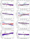 |
Fig. B.1. Oxygen abundance (i.e. 12+log(O/H)) estimations based in the calibration by Marino et al. (2013) as a function of galactocentric distance. Gradients have been derived using the median values estimated for different galactocentric distance intervals. Within each galactocentric distance interval, the median values of the data are represented by blue (red) squares. The blue dots represent metallicity measurements obtained from all the spaxels while the red dots indicate those spaxels where the emission lines are originated in star-forming regions. The blue and red bands indicate the results of our Bayesian linear best fits to the data with the same colour coding as for the individual measurements. The dark and light shaded bands correspond to the confidence intervals at 1-σ and 2-σ levels, respectively. The black dot at the bottom left of the plot represents the median error of all (blue) points. |
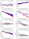 |
Fig. B.1. continued. |
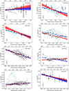 |
Fig. B.1. continued. |
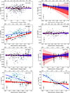 |
Fig. B.1. continued. |
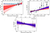 |
Fig. B.1. continued. |
All Tables
Results for the ionised-gas metallicity gradients for the MEGADES sample as functions of the effective radius and galactocentric distance.
All Figures
|
Fig. 1. NGC 3982 concatenated spectra observed with the LR-B, LR-V, and LR-R VPHs in blue, green, and red, respectively. Each spectrum was obtained by combining the 567 individual spectra measured simultaneously with the MEGARA LCB IFU. |
| In the text | |
|
Fig. 2. Flux (top panel) and velocity dispersion (bottom panel) ratios of [O III]λ5007 to [O III]λ4959 as a function of the S/N of [O III]λ4959 measured on the peak of the line using all data included in the MEGADES survey. In both cases, the shaded region between the dashed red lines marks the position of the 10th and 90th percentiles. The solid red line indicates the median value of the flux or velocity dispersion ratio at each S/N value. |
| In the text | |
|
Fig. 3. Panel (a): Pan-STARRS g-band image of the galaxy NGC 0718, with the isophotes calculated using Photutils overplotted in white. Panel (b): Cumulative magnitude derived from the previously measured isophotes as a function of the semi-major axis. Blue dots correspond to the integrated magnitude within each isophote, and the dashed black line is a smoothed interpolation of the distribution. The horizontal solid blue line indicates the asymptotic magnitude of the galaxy, and the orange cross marks the semi-major axis at which the cumulative magnitude reaches a value equal to the asymptotic magnitude plus 2.5log(2), corresponding to the effective radius. Panel (c): Cumulative magnitude as a function of the cumulative magnitude gradient. Each blue dot corresponds to a given isophote. The dashed black line shows a linear fit to the data points at the lowest gradients, and the vertical dashed-dotted black line marks the zero gradient. The intercept of the linear fit with the vertical axis is used to estimate the asymptotic magnitude of the galaxy. |
| In the text | |
|
Fig. 4. Left panels: [O III]λ5007/Hβ versus [N II]λ6584/Hα BPT diagram of all spaxels in the MEGADES sample for galactocentric distance cuts of (from top to bottom): < 0.25 kpc, between 0.25 and 0.5 kpc, between 0.5 and 1 kpc, and > 1 kpc. The size of each point depends on the S/N measured at the peak of the [N II]λ6584 line. The dashed, dotted, dash-dotted, and solid lines represent the Kewley et al. (2001), Kauffmann et al. (2003), Stasińska et al. (2006), and Espinosa-Ponce et al. (2020) demarcation curves, respectively. Right panels: Relationship between [O III]λ5007/Hβ and the velocity dispersion measured on the Hβ line for the same galactocentric distances shown in the left panels. The size of each point depends on the S/N measured at the peak of the Hβ line. Grey dots in the backgrounds correspond to all points in the sample. |
| In the text | |
|
Fig. 5. Left panels: [N II]λ6584/Hα versus the equivalent width of the Hα line for different galactocentric distance cuts (from top to bottom): < 0.25 kpc, between 0.25 and 0.5 kpc, between 0.5 and 1 kpc, and > 1 kpc. The dashed line marks the boundary proposed by Stasińska et al. (2006) to distinguish between star-forming regions (labelled SF) and AGNs. The dotted line indicates the boundary established by Kewley et al. (2006) to separate, within the AGN area, Seyferts from LINERs (labelled L). The dash-dotted line separates the region populated by lines produced in RGs proposed by Cid Fernandes et al. (2011). Right panels: [N II]λ6584/Hα versus velocity dispersion of the Hα line for the same galactocentric distance cuts. In all panels, the size of each point depends on the S/N measured at the peak of the [N II]λ6584 line. Grey dots in the background correspond to all points in the sample. |
| In the text | |
|
Fig. 6. BPT diagrams of [O III]λ5007/Hβ versus [N II]λ6584/Hα (left panel) and [O III]λ5007/Hβ versus ([S II]λ6717+[S II]λ6731)/Hα (right panel). Both panels show the diagrams for three different cuts as a function of the velocity dispersion measured on the Hα line (from top to bottom): < 30 km s−1, between 30 and 70 km s−1, and > 70 km s−1. In the left panel, the dashed, dotted, dash-dotted, and solid lines represent the Kewley et al. (2001), Kauffmann et al. (2003), Stasińska et al. (2006), and Espinosa-Ponce et al. (2020) demarcation curves, respectively. In the right panel, the dashed, dotted, and solid lines represent the Kewley et al. (2001, 2006), and Espinosa-Ponce et al. (2020) demarcation curves, respectively. The size of the points in the left and right panels depends on the S/N measured at the peak of the [N II]λ6584 line and [S II]λ6717, respectively. Grey dots in the backgrounds correspond to all points in the sample. |
| In the text | |
|
Fig. 7. Left panels: Relationship between the measured ratio of velocity dispersions of [N II]λ6584 and Hα lines versus the velocity dispersion on the Hα line for different galactocentric distance cuts. The dashed, dash-dotted, and solid black curves represent lines with a constant broadening with respect to the Hα line of 30, 50, and 70 km s−1, respectively. The dashed orange lines indicate the boundaries between the regions defined by the dynamic selection of excitation mechanisms explained in this section. Right panels: BPT diagram of [O III]λ5007/Hβ versus [N II]λ6584/Hα corresponding to the points falling within each of the regions defined in the left panel. From top to bottom we have the BPT diagram for the lines excited by shocks-like mechanism, photoionisation, and AGNs. The dashed, dotted, dash-dotted, and solid lines represent the Kewley et al. (2001), Kauffmann et al. (2003), Stasińska et al. (2006), and Espinosa-Ponce et al. (2020) demarcation curves, respectively. In both panels blue dots denote lines measured in galaxies classified as Seyfert or LINER (see Table A.1), while the red dots represents the rest of the galaxies. The size of the points depends on the S/N measured at the peak of the [N II]λ6584 line. Grey dots in the backgrounds correspond to all points in the sample. |
| In the text | |
|
Fig. 8. Oxygen abundance (i.e. 12 + log(O/H)) estimations based in the calibration by Marino et al. (2013) as a function of galactocentric distance for the galaxy NGC 3982. Gradients have been derived using the median values estimated for different galactocentric distance intervals. Within each galactocentric distance interval, the median values of the data are represented by blue or red squares. The blue (red) dots represent metallicity measurements obtained from all the spaxels (spaxels whose emission lines originated in star-forming regions; see text). The blue and red bands indicate the results of our Bayesian linear best fits to the data with the same colour coding as for the individual measurements. The dark and light shaded bands correspond to the confidence intervals at 1σ and 2σ levels, respectively. The black dot at the bottom left represents the median error of all the blue points. |
| In the text | |
|
Fig. 9. Metallicity gradients of the ionised gas measured for all galaxies in our sample. The orange circles indicate galaxies that were classified as slow rotators (dynamical classes 1 and 2) and cyan squares indicate fast rotators (classes 3 through 5). Top panel: Gradients computed as a function of galactocentric distance (in kpc). Bottom panel: Gradients computed as a function of the effective radius. The x-axis indicates the y-intercept of the linear fit to the metallicity gradient. Each galaxy is represented twice as we include the results of the best fits obtained using both photoionised spaxels (points with red error bars) and all spaxels (points with blue error bars). |
| In the text | |
|
Fig. 10. Ionised-gas metallicity gradients computed when photoionised-only spaxels are used versus when all spaxels are used. The difference between y-intercepts is shown on the x-axis, while the difference between slopes is included on the y-axis. Orange circles (cyan squares) represent the results of the fits to our slow (fast) rotators. The dashed lines in the central plot mark the zero position on each axis. The thick dashed lines in the frequency histograms mark the median value of the data on each axis. |
| In the text | |
|
Fig. B.1. Oxygen abundance (i.e. 12+log(O/H)) estimations based in the calibration by Marino et al. (2013) as a function of galactocentric distance. Gradients have been derived using the median values estimated for different galactocentric distance intervals. Within each galactocentric distance interval, the median values of the data are represented by blue (red) squares. The blue dots represent metallicity measurements obtained from all the spaxels while the red dots indicate those spaxels where the emission lines are originated in star-forming regions. The blue and red bands indicate the results of our Bayesian linear best fits to the data with the same colour coding as for the individual measurements. The dark and light shaded bands correspond to the confidence intervals at 1-σ and 2-σ levels, respectively. The black dot at the bottom left of the plot represents the median error of all (blue) points. |
| In the text | |
|
Fig. B.1. continued. |
| In the text | |
|
Fig. B.1. continued. |
| In the text | |
|
Fig. B.1. continued. |
| In the text | |
|
Fig. B.1. continued. |
| In the text | |
Current usage metrics show cumulative count of Article Views (full-text article views including HTML views, PDF and ePub downloads, according to the available data) and Abstracts Views on Vision4Press platform.
Data correspond to usage on the plateform after 2015. The current usage metrics is available 48-96 hours after online publication and is updated daily on week days.
Initial download of the metrics may take a while.