| Issue |
A&A
Volume 705, January 2026
|
|
|---|---|---|
| Article Number | A54 | |
| Number of page(s) | 20 | |
| Section | Extragalactic astronomy | |
| DOI | https://doi.org/10.1051/0004-6361/202556217 | |
| Published online | 07 January 2026 | |
Multi-messenger observations of binary neutron star mergers: Synergies between next-generation gravitational wave interferometers and wide-field, high-multiplex spectroscopic facilities
1
LUX, Observatoire de Paris, Université PSL, Sorbonne Université, CNRS, 92190 Meudon, France
2
INAF – Osservatorio Astronomico d’Abruzzo, 64100 Teramo, Italy
3
Gran Sasso Science Institute (GSSI), I-67100 L’Aquila, Italy
4
INFN, Laboratori Nazionali Del Gran Sasso, I-67100 Assergi, Italy
5
National Centre for Nuclear Research, Pasteura 7, PL-02-093 Warsaw, Poland
6
Institute of High Energy Physics – Austrian Academy of Sciences, 1010 Vienna, Austria
7
Institute of Physics, Laboratory of Astrophysics, École Polytechnique Fédérale de Lausanne (EPFL), Observatoire de Sauverny, 1290 Versoix, Switzerland
★ Corresponding author: This email address is being protected from spambots. You need JavaScript enabled to view it.
Received:
2
July
2025
Accepted:
3
October
2025
Abstract
Context. Third-generation gravitational wave (GW) observatories, such as the Einstein Telescope (ET) and Cosmic Explorer (CE), will access a large volume of the Universe, and detect hundreds of thousands of binary neutron star (BNS) mergers, reaching distances beyond z ∼ 3. The unique information revealed by joint GW and electromagnetic (EM) detections can be fully exploited only with a dedicated observing strategy and suitably adapted EM facilities.
Aims. In this work, we explore the impact of integral field and multi-object spectroscopy (IFS and MOS) with the Wide-field Spectroscopic Telescope (WST) on the detection of EM counterparts from BNS detected by next-generation GW observatories.
Methods. We considered populations of BNS mergers assuming different equations of state and mass distributions. We computed the corresponding GW signals for both the ET operating alone and in a network with CE. Kilonova (KN) light curves were assigned using either AT2017gfo-like models or numerical-relativity-informed ones. Gamma-ray burst (GRB) afterglow emission was also included. We considered two main observing strategies: one in synergy with wide-field photometric surveys and a second based on a galaxy-targeted approach, exploiting WST’s high multiplexing capabilities. We also estimated the number of galaxies within the GW error volume. Here, we discuss potential observational challenges and corresponding mitigation strategies.
Results. We find that KNe from BNS mergers can be detected with WST up to z ∼ 0.4 and magnitudes mAB ∼ 25, while GRB afterglows may be observable at higher redshifts, z > 1, for viewing angles of Θview ≲ 15°. We show that Target of Opportunity (ToO) observations aimed at KN detections can be optimally scheduled 12–24 hours after the merger. For GRB afterglows, particularly in cases of a poor localisation in the first minutes after the high-energy detection, WST IFS can play a key role in counterpart identification and position refinement. Our results show that mini-IFUs (fibre bundles) and galaxy catalogues that are complete in redshift up to z ≤ 0.5 will be essential for the efficient identification of EM counterparts. We find that the WST contribution is also valuable for events with good sky localisation because the uncertainties in luminosity distance (even at low redshift) can result in large error volumes containing numerous galaxies to target up to several thousands at z < 0.1 and tens of thousands at z < 0.2 for GW detections of ET in a network with CE. Finally, we underline that events at redshifts of z < 0.3 and with sky localisations better than 10deg2 will be ‘golden’ events for WST, making it become possible for WST to cover all the galaxies in the error volume with a limited number of exposures. We estimate these to range from about ten (ET-alone configuration) to hundreds per year (ET + CE configuration).
Conclusions. The detection and characterisation of EM counterparts of BNS mergers explored by next-generation interferometers will be challenging. Observational strategies and selection criteria should be defined in advance to prioritise events for follow-up among the potentially thousands per year expected from ET and CE. Detecting their EM counterparts will require facilities capable of covering sky regions of tens of deg2, reaching depths of AB > 22, and rapidly gathering the data needed to identify the many candidate sources expected for each event. We have shown that spectroscopic facilities with large fields of view, high sensitivity, and high-multiplexing modes are powerful instruments to successfully exploit the new multi-messenger science opportunities that will be opened up thanks to next-generation GW interferometers.
Key words: gravitational waves / instrumentation: spectrographs / binaries: general / gamma-ray burst: general
© The Authors 2026
 Open Access article, published by EDP Sciences, under the terms of the Creative Commons Attribution License (https://creativecommons.org/licenses/by/4.0), which permits unrestricted use, distribution, and reproduction in any medium, provided the original work is properly cited.
This article is published in open access under the Subscribe to Open model. This email address is being protected from spambots. You need JavaScript enabled to view it. to support open access publication.
1. Introduction
The extraordinary joint detection of gravitational waves (GWs) and light from a binary neutron star system merger (BNS) on 17 August 2017 (Abbott et al. 2017a) initiated the era of GW multi-messenger (MM) astrophysics. That day, GWs from a BNS merger at a luminosity distance of ∼40 Mpc were detected by Advanced Ligo and Virgo detectors, which localised the source within a 28 deg2 credible region (Abbott et al. 2017b). After ∼1.7 seconds a short gamma-ray burst (SGRB) was detected by Fermi and INTEGRAL satellites (Goldstein et al. 2017; Savchenko et al. 2017; Abbott et al. 2017c). This sparked an extensive multi-wavelength EM follow-up campaign: a few hours later, telescopes from all over the world were tiling the GW sky localisation, including galaxy targeted searches. They discovered a faint, fast-evolving optical transient in the galaxy NGC4993 (e.g. Coulter et al. 2017; Lipunov et al. 2017; Soares-Santos et al. 2017; Tanvir et al. 2017; Valenti et al. 2017) whose redshift was consistent with the GW source luminosity distance. Subsequent monitoring of the source light curve and spectrum (e.g. Villar et al. 2017; Nicholl et al. 2017), especially the spectroscopic observations taken with VLT/X-shooter from ∼1.4 days after the GW detection, enabled the classification of the transient as a kilonova (KN; Pian et al. 2017; Smartt et al. 2017), that is, thermal radiation powered by the radioactive decay of r-process heavy elements produced in the neutron-rich ejecta environment, favored by the merger of the two neutron stars (NSs). In addition, from ∼10 days post-merger onwards, a broad-band non-thermal source was detected at the very same position of the KN. Thanks to VLBI proper motion measurements and to radio and X-ray campaigns, it is now known to be the off-axis afterglow produced by the structured jet of SGRB170817A (Mooley et al. 2018, 2022; D’Avanzo et al. 2018; Margutti et al. 2018; Ghirlanda et al. 2019). This plethora of observations confirmed the theoretical hypothesis that at least part of SGRBs originate in BNS mergers. At the same time they raised many questions concerning, for instance, the nature of heavy elements produced in these violent explosions, the population of KN in all its variety, and the link between BNS and SGRBs. Moreover, the study of joint GW-EM detections has implications in various fields: from cosmology, allowing for independent estimates of the Hubble constant to be undertaken (Abbott et al. 2017d; Guidorzi et al. 2017; Hotokezaka et al. 2019; Bulla et al. 2022), to the study of GRB jet structure (e.g. Lazzati et al. 2017; Troja et al. 2018; Lamb et al. 2019; Ghirlanda et al. 2019; Salafia & Ghirlanda 2022). Unfortunately, no analogous opportunity to observe simultaneously these two cosmic messengers has arisen thus far. Before the start of the fourth observing run (O4) of the LIGO/Virgo/KAGRA (LVK) detectors, the expected detection rate of BNS was  yr−1 (Abbott et al. 2020a). Unfortunately, no BNS detection was reported during the O4 run to date.
The situation demonstrates that predicted and effective detection rates of BNS with current GW interferometers are still very low. However, with next-generation GW observatories, such as the Einstein Telescope (ET; Punturo et al. 2010) and Cosmic Explorer (CE; Reitze et al. 2019), they will dramatically increase. With ET alone it will be possible to detect up to ∼105 BNS per year well beyond the Local Universe (Branchesi et al. 2023; Abac et al. 2025). The majority of sky localisation regions of such events will be large and the EM counterparts will be faint. Facilities that combine high sensitivity with wide fields of view (FoVs), such as the Vera Rubin Observatory for photometry, will be indispensable for the research of the EM counterparts. Spectroscopic observations, fundamental to identifying and characterising the counterpart candidates (and therefore to discriminate among them) will likely be the bottle-neck of GW MM science.
In this work, we explored the use of integral field and multi-object spectroscopy (IFS and MOS) for the search and identification of EM counterparts of GW detections from next-generation GW interferometers such as ET. Overall, IFS and MOS offer a significant advantage by enabling the simultaneous acquisition of multiple spectra. An IFS captures a spectrum at each spatial pixel within a two-dimensional (2D) field, enabling simultaneous spatial and spectral coverage over a compact region of the sky. In contrast, MOS acquires spectra from multiple individual targets across a wide FoV in a single exposure, typically using optical fibres.
To date, the best project integrating such facilites is the Wide-field Spectroscopic Telescope (WST; Bacon et al. 2024; Mainieri et al. 2024), a concept study to be realised in the southern hemisphere in the 2040s, overlapping with ET operations. WST will be equipped both with a panoramic IFS, having a FoV that is nine times larger than that of MUSE, 30 000 low-resolution fibres and 2000 high-resolution fibres (MOS). It is envisioned as a dedicated 12-meter-class spectroscopic facility, having time-domain and multi-messenger among the structuring science cases.
We use simulations of BNS detections datasets and corresponding KN and GRB afterglow emission (described in Sect. 2) to explore the observations with WST IFS and MOS (Sect. 3). We study the detectability and characterisations with WST of such EM counterparts, and we investigate how the results depend on the observable and intrinsic properties of the BNS population (Sect. 4). Finally, we discuss different observing strategies, examine potential observational challenges, and explore some selection criteria (Sect. 5). We summarise our results in Sect. 6. Throughout this paper, we assume a flat ΛCDM cosmology with H0 = 67.66 km s−1 Mpc−1, ΩM = 0.3 (Planck Collaboration VI 2020).
2. EM counterparts of BNS mergers detected by ET and CE
To model the KN and SGRB afterglow signals associated with detections of BNS mergers by ET and CE, we considered three different datasets, presented in Sect. 4.3 of Branchesi et al. (2023) (set 1) and in Loffredo et al. (2025) (set 2 and set 3). The KN associated with the GW-detected mergers in set 1 were modelled on the basis of AT2017gfo, the only KN detected in association with GWs so far. Specifically, among the models published in the literature (e.g. Kasen et al. 2017; Perego et al. 2017; Villar et al. 2017), we adopted the KN model from Perego et al. (2017), using the best-fit parameters for AT2017gfo reported in that work. Each KN light curve was then modified to account for the binary inclination angle, luminosity distance, and the resulting cosmological corrections. In this way, we were able to obtain a population of KNe resembling AT2017gfo, but distributed at different distances and observed from different viewing angles. For this reason, hereafter we refer to this set of KN as gfo-like KN sample. Instead, KN light curves associated with BNS mergers in set 2 and 3 were computed on the basis of results from numerical-relativity simulations targeted to GW170817 and GW190425 (Abbott et al. 2020b), the second BNS merger detected by LVK. Additionally, sets 2 and 3 include SGRB afterglow emission. Despite being more model-dependent, sets 2 and 3 account for the expected diversity in KN signals from a population of BNS mergers, which can realistically differ significantly from GW170817. To distinguish these two datasets from the gfo-like KN one, we call hereafter the KN populations following these mergers the theoretical KN sample. Below, we briefly overview the three datasets, whose characteristics are summarised in Table 1. Some additional information is reported in Appendix A and we refer to Branchesi et al. (2023) and Loffredo et al. (2025) for more details. We note that in the literature there is another set of simulations of ET BNS detections, along with their associated KN and afterglow populations, presented in Colombo et al. (2025).
Characteristics of the different simulated datasets used for our study.
2.1. BNS, GW detection, and KN population simulations: Set 1
The starting BNS merger population is documented in Santoliquido et al. (2021) and corresponds to a local merger rate ℛBNS = 365 Gpc−3 yr−1-pagination
(common envelope parameter α = 3), which is compatible with the 90% credible interval of ℛBNS-pagination
∈[10 − 1700] Gpc−3 yr−1 reported in GWTC-3 (Abbott et al. 2023a). From this population, Ronchini et al. (2022) and Branchesi et al. (2023) built a catalogue of one year of BNS mergers, corresponding to 9 × 10⁵ BNS mergers observable by Earth with an ideal instrument. The two NS masses in each binary of the catalogue were assigned by randomly sampling a uniform distribution between 1 and 2.5 M⊙ in agreement with GWTC-3 results (Abbott et al. 2023b). Each NS has a dimensionless tidal deformability sampled from a uniform distribution between 0 and 2000 (Abbott et al. 2023b). All BNS mergers in the catalogue are distributed isotropically in the sky with a random inclination of the orbital plane with respect to the line of sight (LoS). Given this catalogue of BNS mergers, Branchesi et al. (2023) simulated one year of observations by ET operating at full sensitivity (xylophone configuration) in two possible geometries (triangular with 10 km arms and 2L with 15 km arms), assuming 85% uncorrelated duty cycle for each of the nested interferometers in ET. The analysis conducted with GWFish (Dupletsa et al. 2023) produced the detector S/N and source parameters, along with relative errors for each source, including the sky-localisation uncertainty, Ω90, defined as the 90% credible region. Finally, they associated a KN light curve in the ugrizy filters of the Vera Rubin Observatory (Rubin hereafter) with each merger detected with S/N > 8.
Within this sample, we selected all the KN light curves corresponding to mergers detected with S/N > 8 and localised better than 100deg2. The arbitrary cut on the sky localisation was chosen to limit the computation time due to the large number of events and it is based on the unlikeliness that optical telescopes would follow GW events with larger sky localisations.
We notice that this KN modelling, based on a black body approximation, leads to an overestimation of the UV component (Gillanders et al. 2022; Ricigliano et al. 2024). Therefore, when we build rough spectra from the photometry, as outlined in Sect. 3, we correct the overestimation in the UV to correctly reproduce AT2017gfo. All the details of the correction are provided in Appendix A.
2.2. BNS, GW detection and KN population simulations: Sets 2 and 3
The original BNS merger population is reported in Iorio et al. (2023), predicting a local merger rate ℛBNS = 107 Gpc−3 yr−1 (common envelope parameter α = 1). This merger rate is compatible with the 90% credible interval ℛBNS ∈ [10 − 1700] Gpc−3 yr−1 reported in GWTC-3 (Abbott et al. 2023b). Starting from this population, Loffredo et al. (2025) built four catalogues of ten years of BNS mergers up to redshift z = 1, considering two possible NS mass distributions, namely, a Gaussian and a uniform distribution, and two possible NS equations of state (EoSs), namely, APR4 (Akmal et al. 1998; Baym et al. 1971; Douchin & Haensel 2001) and BLh (Bombaci & Logoteta 2018; Logoteta et al. 2021).
The Gaussian mass distribution is centred at 1.33 M⊙ with a standard deviation of 0.09 M⊙ and reproduces the distribution of BNSs in our galaxy (Özel et al. 2012; Kiziltan et al. 2013; Özel & Freire 2016). The uniform distribution ranges between 1.1 M⊙ and a maximum mass Mmax set by the NS EOS. Specifically, the maximum mass is 2.2 M⊙ for the APR4 EOS and 2.1 M⊙ for BLh. For each binary, the dimensionless tidal deformability was assigned by considering the NS mass and EOS. As for set 1, the mergers in the catalogues are distributed isotropically in the sky with a random inclination of the orbital plane. For each catalogue, Loffredo et al. (2025) simulated ten years of observations by ET (xylophone configuration) in two possible geometries (triangular or 2L) operating alone (set 2) or in a network with one CE interferometer (1CE, set 3), providing the parameter estimation performed with GWFish (Dupletsa et al. 2023) and the sky-localisation uncertainty obtained by each GW detector network. Then, they associated KN light curves in the griz filter of Rubin with mergers detected with S/N > 8. The KN modelling assumes an anisotropic KN ejecta with two components of differing opacities, reflecting their different compositions–one being more lanthanide-rich than the other. This leads to a viewing angle dependent color evolution. In addition, prompt collapse to a black hole (BH) affects the color evolution by suppressing the blue polar component. The ejecta properties are computed through numerical relativity-informed fitting formulas. Additionally, the model considers the effect on KN light curves induced by prompt collapse of the merger to black hole (BH), which is more likely for massive and asymmetric binaries.
The model was calibrated to reproduce KN light curves compatible with AT2017gfo for BNS mergers with chirp mass and mass ratio similar to GW170817. However, it also takes into account diverse KN light curves associated with BNS possibly different from GW170817. KN light curves are informed with the properties of the NS EOS, predicting, in general, brighter KN light curves for the BLh EOS compared to the APR4 EOS. As for set 1, the light curves are computed considering cosmological and K corrections. Finally, the catalogues from Loffredo et al. (2025) include the emission from the optical afterglow of short GRBs possibly produced during the mergers. The modelling of the jet is based on SGRB170817A (Ghirlanda et al. 2019) and SGRBs observed so far (Ronchini et al. 2022). The optical afterglow is computed through the Python package afterglowpy (Ryan et al. 2020), using as parameters ϵe = 0.1, p = 2.2, log10ϵB uniformly distributed in the range [ − 4, −2] and n ∈ [0.25, 15] × 10−3 cm−3. This modelling reproduces the observed range of the optical fluxes of short GRBs (Kann et al. 2011). The fraction, fj, of BNS mergers that can produce a GRB is still uncertain. It is specific to the BNS population considered and calibrated to match the observed local SGRB rate. We adopted the SGRB rate from Ghirlanda et al. (2016). For our BNS population sets fj = 0.7, so that a GRB afterglow light curve is assigned to 70% of the BNS mergers in our catalogue.
From these catalogues, we selected all the BNS mergers detected with S/N > 8 and localised better than 100deg2, for ET operating alone, and 40deg2, for ET operating in a network with 1CE, and the associated KN and SGRB afterglow light curves. The smaller threshold used for the network including ET and CE takes into account the larger number of relatively well-localised detections and the limited observational time resources of optical telescopes.
Figure 1 shows the magnitude distribution of the optical counterparts presented in this section (set 2 and set 3) for a 2L configuration) at ∼12 hours post-merger. The brightness of KNe, along with on-axis and slightly off-axis afterglows in our populations, decreases rapidly with increasing distance, and KNe observed to date have sampled only the brightest portion of the total population expected across cosmic time.
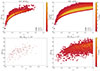 |
Fig. 1. AB magnitude in Rubini filter at ∼12 hours post-merger as a function of redshift for KNe and on-axis (θview < 15°) GRB afterglows following BNS detected by ET as a stand-alone observatory (left panels) and in a network with CE (right panels). The few bright KNe (mAB < 21) in the upper-right panel are not visible due to their low density relative to the bulk of the population, which dominates the color scale. The cross, upwards pointing triangle, and star respectively represent AT2017gfo, and the optical counterparts of GRB 211211A (Rastinejad et al. 2022) and GRB 230307A (Levan et al. 2024), two GRBs followed by a KN, at ∼12 hours after the GRB prompt detection. A Gaussian filter was applied to the data in the top panels and bottom-right one for visualisation purposes. |
3. WST simulations
We performed simulations of WST observations to study the characteristics of the population that is detectable with WST, independently of any detailed operational strategy of WST observations in general, whose preparation and study are among the goals of this work. We provide the definition of detectability with WST (mainly based on a S/N threshold) later in this section. For the purposes of this paper, we did not aim to simulate the KN spectral features, but the rough overall brightness of the continuum. This paper focuses on detectability of the EM counterparts with WST: a detailed analysis of spectral features is beyond the scope of this work.
For set 2 and set 3, Loffredo et al. (2025) outlined an observing strategy to adopt with Rubin to research the EM counterparts. According to this strategy, an event is classified as detectable with Rubin if it is observed in at least one epoch in both g and i filters, with exposures lasting 600 seconds. The observing strategy takes into account for the Observatory footprint and the sources position (RA, Dec) in the sky that are observed from the Chilean site of Cerro Pachón.
Other Rubin strategies for GW counterpart searches (e.g. Margutti et al. 2018; Bianco et al. 2019; Andreoni et al. 2024) typically employ a larger number of filters and shorter exposures (of the order of 30s–180s). They are optimised for the current generation of GW detectors and developed in the context of ToOs interrupting the ongoing LSST survey. The observational strategy considered in Loffredo et al. (2025) is targeted at the 3G GW observatories era, supposing that the LSST survey will be completed.
We adopted a two-filter (g and i) strategy to capture the color evolution of the KN (choosing i over z filter to achieve better depth) and proposed longer exposures of 600 s to detect fainter KNe. To simulate WST detections within set 2 and set 3, we used the subsample of the KN and GRB afterglow populations that would be detectable by Rubin, considering that both WST and Rubin sites should be in the southern hemisphere, as well as the slightly deeper magnitude detectable by Rubin.
The simulations of WST observations were performed with the WST Exposure Time Calculator (ETC)1, properly modified to adapt it to this specific science case. In particular, we added to the Python source code functions to create artificial rough spectra and to analyse different input spectra. With the ETC, we simulated the signal to noise ratio (S/N) per spectel (i.e. spectral pixel) for WST IFS and MOS low-resolution spectrograph (see Table 2) of KN and GRB afterglow emission following the BNS mergers in our samples.
Some characteristics of the WST IFS and MOS channels used in this study.
We used simulated photometric data in Rubin filters of KN and GRB afterglows to build artificial rough spectra of each EM counterpart over time. We started from the simulated AB magnitudes in Rubin filters – g, r, i, and z for the theoretical sample and ugrizy for the gfo-like one (to which we added the contribution of Galactic dust extinction). Then we converted them into observed flux density (er s−1 cm−2 Å−1) at each filter effective wavelength, approximately considered as the medium flux in that filter. Thus, we obtained a dataset of 4 (6) flux density values at 4 (6) different wavelengths for each event at each time step: the fit of these values with a quartic (sextic) polynomial was used as input spectrum of WST simulations. Once we had rough spectra both for the gfo-like KN and theoretical KN samples, we computed the S/N over the best throughput wavelength range of WST IFS and MOS channels. The S/N of MOS was spatially integrated over the fibre aperture (1″ assumed in version 0.31 of the ETC), while for the IFS we used a specific function of the ETC, computing the optimum aperture diameter that maximises the S/N.
We consider an event ‘detectable’ when the average S/N in the selected spectral range exceeds a threshold of 3. We assume a seeing of 0.7″ and an airmass of 1 as observing conditions. These are optimal observing conditions, but a detailed analysis goes beyond the scope of this work. In the sections that follow, we show and discuss the properties of the BNS populations and their detectable counterparts, sampled at approximately 3, 6, 12, 24, 48, and 72 hours (observer frame) after the merger. We consider exposures lasting 1800 s and 3600 s: we present results for 3600 s exposures in the main section and give those for 1800 s in Appendix B.
4. WST-detectable EM counterparts
The results presented in the following sections do not depend on the configuration chosen for ET. Therefore, we decided to show only those based on the simulation of the population detected by the 2L design. Similarly, we did not observe any significant differences in terms of the redshift horizon, median magnitudes, detectability trends over time, or other observable properties relevant to assessing the impact of IFS and MOS with WST, across the four combinations of NS EoS and mass distributions considered. Differences do emerge in the total number of detections, but they are aligned with those already discussed in Loffredo et al. (2025), without introducing additional dependencies. Therefore, we give our results for the BLh EoS and the Gaussian mass distribution only.
4.1. Detectable fraction and best observing time post trigger
The percentage of detectable EM counterparts primarily depends on time elapsed since the merger and the instrument used (with IFS being slightly more performative in this regard with respect to fibres). Figure 2 shows the detectable percentages of gfo-like and theoretical KN as a function of time, using WST fibres. Results for the IFS are shown in Fig. C.1. As expected, KNe become fainter in the g band with respect to the i band at late epochs (see also Fig. C.5); hence, the detectability improves in the redder bands. To maximise the probability of detection, the best time to trigger observations appears to be from about 12 hours to 1 day after the merger, as this is when the highest detectability is achieved, independently of the spectrograph channel and mode. This estimate already accounts for the diversity of KN signals expected from BNS mergers with different neutron star equations of state and masses, leading to a range of ejecta masses and compositions. This includes the effects of the viewing angle on the colour evolution. We also note that observations in the blue channel are preferred only if they start within a few hours after the trigger.
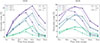 |
Fig. 2. Percentage of gfo-like KNe (left) and theoretical KNe (right) following BNS mergers detected by ET in the 2L configuration that are detectable with WST MOS. Different colors indicate different S/Ns; dashed, dotted, and solid lines correspond to the blue, orange, and red arms of the spectrographs, respectively. The highest detectability occurs approximately 12–24 hours post-merger. The peak time of the detectability reflects the optimal observational window across the full range of ejecta masses, compositions, and inclinations considered in our simulations. |
In Fig. 3, we show the fraction of the WST MOS detectable events at 12 hours after the BNS merger as a function of their magnitude. Results for the IFS are reported in Fig. C.2. With WST, it will be possible to detect KNe having i-band magnitudes as faint as ∼25 with fibres and ∼25.5 with the IFS with one-hour exposures (see Fig. C.3 for the analogous figure for the g band). The bright sources that have not been detected were mainly missed because they were not located in the sky-coverage of VRO and WST, representing nearly 30% of the bright (mag < 22) KN population. In Appendix D we report some details on the comparison of the performances of current MOS facilities, such as 4MOST and WEAVE, and WST.
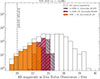 |
Fig. 3. Magnitude distribution in i filter of ET BNS detected over 10 years and their corresponding theoretical KN at ∼12 hours after the merger. The background distribution in white corresponds to the parent BNS + KN population. The colored distributions correspond to the EM counterparts that are detectable with the WST MOS red arm, with different colors corresponding to different S/N intervals. The dashed vertical line indicates the approximate magnitude limit of current MOS facilities, such as 4MOST and WEAVE, for a one-hour exposure. |
4.2. Properties of the KN population detectable at 12 hours post-merger
Here, we present the results at 12 hours post-merger as, on average, this is when the highest detectability is achieved (Fig. 2). Figure 4 shows the redshift distribution of ET BNS events and their corresponding theoretical KNe approximately 12 hours post-merger, along with the distribution of KNe detectable using WST fibres. The detection limit with fibres is around z ∼ 0.35, while the IFS allows for detections up to z ∼ 0.4 (see Fig. C.4 for the redshift distribution using WST IFS).
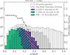 |
Fig. 4. Redshift distribution of ET BNS detected over 10 years and the corresponding theoretical KN at ∼12 hours after the merger. The background distribution in white corresponds to the parent BNS + KN population. The colored distributions correspond to the EM counterparts that are detectable with WST MOS blue or orange or red arm, different colors corresponding to different S/N intervals. EM counterparts detectable with Rubin are shown in grey. Black points refer to the y axis ticks on the right hand side and show the fraction of detectable (S/N > 3) EM counterparts, with no additional information on the S/N range, with respect to Rubin detections. |
A crucial factor that will influence the choice of the observing strategy and the real chances for these electromagnetic counterparts to be observed is the sky-localisation uncertainty, Ω90. The Ω90 value of BNS detected by ET alone rapidly worsens with increasing redshift and covers regions as small as a fraction of deg2, up to the maximum limit of 100deg2 that we imposed. A network including ET and CE benefits from improved sky localisation at higher redshifts and results in a significantly higher number of well localised events at lower redshift (Fig. 5).
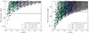 |
Fig. 5. Sky localisation uncertainty as a function of redshift of BNS (white points) detected with ET (left panel) and ET + CE (right panel) over 10 years. Grey points refer to the EM counterparts detectable with Rubin, among which the colored points refer to those that are detectable with WST IFS blue arm at ∼12 hours post-merger. Different colors correspond to different S/N. Percentage reported in the legend refer to the fraction of EM counterparts that are detectable with WST, with respect to those that are detectable with Rubin. The black dashed line represents WST patrol area, 3.1 deg2, where fibres will be positioned. |
The last property we want to explore in this context is the viewing angle, Θview, of the BNS, which is the angle between the BNS angular momentum axis and the LoS. Figure 6 shows the population of BNS detected by ET alone and in a network with CE, highlighting those whose counterparts are detectable with WST. As redshift increases, there is a noticeable absence of edge-on systems. This happens because the S/N of the GW signal is higher for face-on systems compared to edge-on systems with the same intrinsic parameters. Given the spectral range of the best throughput considered for the IFS channel (see Table 2), there is no strong difference in the viewing angle dependence of the detectability for observations in the blue or red bands. This dependence becomes important in the MOS case if its blue and red channels are considered, especially for observations taken after ∼1 day from the GW detection. In this case, the blue channel worsens its efficiency in detecting the EM counterpart of ∼15% compared to the red one, when moving from Θview = 0° to Θview = 45°. The orange channel behaves similarly to the red one.
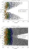 |
Fig. 6. Viewing angle as a function of redshift of theoretical KN following BNS mergers (white points) detected by ET alone (top panel) and ET in a network with CE (bottom panel). Colored points represent WST detections, different colors corresponding to different S/N. The lack in GW detections for edge-on systems is due to GW signal S/N, that is higher for face-on systems with respect to edge-on systems with the same intrinsic parameters. |
When considering ET alone, WST does not detect edge-on systems beyond z ∼ 0.1. However, this limitation is only due to the redshift distribution of the GW-detected BNS population with respect to the viewing angle.
The dependence of sky localisation on the viewing angle is relatively weak for BNS GW detections, although it tends to worsen for edge-on systems due to their lower S/N. Therefore, large FoV and high multiplexing facilities can be necessary for the spectroscopic follow-up independently of the viewing angle of the BNS event (see, however, Sect. 4.3 for the case of well localised on-axis GRB afterglows).
4.3. GRB afterglow contribution
One of the expected EM counterparts from BNS mergers are GRB afterglows (both on- or off-axis). We studied the afterglow detectability by WST, using the afterglow simulations reported in Sect. 2.2. We considered different observing times from 3 hours to 3 days post-merger, for BNS detected by ET in a network with CE. We found that the contribution of the afterglows is mainly limited to on-axis and slightly off-axis systems (Θview < 15°; see Table 3 and Fig. C.6). More than 90% of the events with Θview < 10° have afterglows that outshine the KN and are detectable with WST (see Fig. 7 for the 12 hours and 3 days cases), at any of the considered times. The fraction decreases significantly for larger viewing angles and later observations, becoming null at Θview ∼ 20°.
Percentage of afterglows outshining KNe in different bins of a viewing angle, Θview, at different times post-merger.
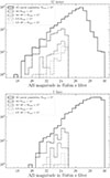 |
Fig. 7. Magnitude distribution in the Rubini filter (with a cut at m = 30) of afterglows produced by BNS mergers with a viewing angle below 15° (solid black line), at ∼12 hours (top panel) and ∼3 days (bottom panel) post-merger. Dashed- and dot-line black histograms correspond to events that are detectable with WST (i.e. where the combined flux of the afterglow and KN has S/N > 3) and for which the afterglow outshines the KN, for Θview < 10° and 10° < Θview < 15°, respectively. Dashed- and dot-line gray histograms represent detectable events where the kilonova dominates over the afterglow, for Θview < 10° and 10° < Θview < 15°, respectively. |
We stress that (in contrast to KN) afterglows with Θview ∼ 15° can be detected by WST (see also Fig. C.6) also for events beyond z = 0.4 (even beyond z = 1). For such cases, the possibility of a detection is optimized by observations starting as soon as possible after the merger, because the optical light curves of on-axis afterglows are initially brighter than KNe and later fade, following a power-law decay. Our simulations show that at 12 hours the fraction of detectable afterglows with Θview ∼ 15° is reduced by half compared to the case of observations starting 3 hours after the merger.
Spectroscopic follow-up with WST is well suited for both on-axis and off-axis systems, albeit with some differences. The use of WST large number of fibres to identify the EM counterpart of an on-axis BNS will not be necessary when the GRB prompt emission has already been detected by satellites capable of detecting and providing rapid precise localisations of GRBs and their afterglows (supposing that such satellites will be operational in the 2040s). However, deploying the IFS on the GRB localisation remains extremely valuable in case of localisations spanning several arcminutes to obtaining spectra of the field, besides those of the counterpart itself. This enables the measurement of redshifts for galaxies in the field, particularly relevant for BNS systems with significant offsets from the centres of their host galaxy (see Sect. 5.2). This facilitates both the identification of the host galaxy and the spectroscopic characterisation of the counterpart itself. For the case of slightly off-axis GRBs and afterglows (θjet < 15°), where a precise enough localisation may not be available, WST high multiplexing capability becomes crucial for identifying the EM counterpart.
5. Observing strategy
We considered two possible observing strategies to adopt with WST to search EM counterparts of BNS GW signals from next generation observatories. We outline them in the following section and we also investigate their feasibility, the possible issues, and the expected outcomes. For both strategies, telescope-level ToOs were considered. The first strategy consists of exploring the GW signal error region with WST alone, performing a galaxy targeted research, possibly covering the peak of the probability regions with the IFS and the remaining area with fibres. The second strategy we considered was to use WST in synergy with optical-NIR photometric observations, targeting the EM counterpart candidates that they will provide.
In this work, we have only considered galaxy selections made on the basis of redshift and not any other additional properties, such as stellar mass and star formation rate (SFR), as this is beyond the scope of our study. We note that despite selections based on high values of stellar mass or SFR have been used for the searches of EM counterparts of BNS detected by LVK, those are not the typical properties of SGRB host galaxies, which actually span different values of star formation rate and stellar mass (Fong & Berger 2013; Berger 2014; D’Avanzo 2015; Nugent et al. 2022).
5.1. Galaxy-targeted research in a stand-alone scenario
In the perspective of performing galaxy-targeted searches of the EM counterparts within the 3D error volume of the GW signal, we aim to give an estimate of the number of galaxies that can be found within such volumes. For this exercise, we supposed that the relevant information on the photometric or spectroscopic redshift of galaxies would be available from previous surveys or from the WST galaxy surveys. We underline the importance of galaxy catalogue completeness to obtain unbiased results.
First, we selected the BNS with z < 0.45, as this corresponds to the detection horizon of the potentially associated KN. We did not apply here any further pre-selection based on which events are detectable with Rubin or WST. Then we estimated the 3D error region of each of them as follows. We consider the differential comoving volume,
 (1)
(1)
where E(z) and DH are defined as
and DA is the angular diameter distance, as defined in Hogg (1999).
We multiplied the differential comoving volume by the uncertainty on the sky localisation of the BNS (2D error area) and we integrated this product over redshift to obtain the 3D error region, which we refer to as the comoving error volume (V; see Fig. 8). The GW analysis provides one value of DL and corresponding error ΔDL for each BNS. To define the bounds of the integral, we converted DL − ΔDL and DL + ΔDL into redshift values (z1 and z2). If ΔDL > DL, we set z1 = 0 as the lower bound. We note that ΔDL depends on the source location in the sky and that, on average, the sky localisation and ΔDL worsen with redshift. However, we stress that large error volumes containing a huge number of galaxies can be found even at low redshift (See Figs. C.8 and C.9).
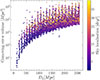 |
Fig. 8. Comoving error volume as a function of GW luminosity distance for each BNS detected by ET in a network with CE at z < 0.45. The color of the points refers to the uncertainty on the sky localisation, according to the color bar on the right. |
To estimate the number of galaxies within the comoving error volume of each BNS, we multiplied this volume by the galaxy number density, computed by integrating the galaxy luminosity function (GLF) in different magnitude intervals. The basic shape of GLF is given, in terms of absolute magnitude, M, as a single Schechter function,
![Mathematical equation: $$ \begin{aligned} \Phi (M) = 0.4 \cdot \ln (10) \cdot \Phi ^{*} \cdot 10^{0.4(\alpha + 1)(M^{*} - M)} \exp \left[-10^{0.4(M^{*}-M)}\right] ,\end{aligned} $$](/articles/aa/full_html/2026/01/aa56217-25/aa56217-25-eq4.gif) (2)
(2)
where M* is the characteristic absolute magnitude, α represents the faint-end slope parameter, and Φ* is a normalisation constant giving the number of galaxies per Mpc3 (Schechter 1976). Here, Φ(M) can be written in terms of the apparent magnitude, m, as
![Mathematical equation: $$ \begin{aligned} \Phi (m)&= 0.4 \cdot \ln (10) \cdot \Phi ^{*} \cdot 10^{0.4(\alpha + 1)(M^{*} - m + 5\log _{10}(D_{\mathrm{L} }) - 5)} \nonumber \\&\quad \times \exp \left[-10^{0.4(M^{*} - m + 5\log _{10}(D_{\mathrm{L} }) - 5)}\right] ,\end{aligned} $$](/articles/aa/full_html/2026/01/aa56217-25/aa56217-25-eq5.gif) (3)
(3)
where DL is the luminosity distance in parsec. We assume that once DL is fixed, Φ(m) gives the number of galaxies per unit apparent magnitude per unit volume [Mpc−3] at that DL, and remains nearly constant in redshift across the comoving error volume. Hence, for each event we integrate Φ(m) over different magnitude intervals. Then, we multiplied the number density of galaxies in each magnitude bin by the comoving error volume. We used the Schechter function parametrisation from Ilbert et al. (2005) for redshifts of 0.05 < z < 0.5.
Figure 9 shows the number of galaxies within the comoving error volume of the BNS detected by ET observing alone and in a network with CE as a function of redshift. The number density is derived from the GLF in the I band. Figure 10 shows the number of galaxies within the comoving error volume of the same events, as a function of sky localisation. Also, if we initially assume that each galaxy will be targeted with ∼1 fibre, we can compare the number of galaxies with the number of WST fibres that can potentially be used. If the 2D error region of the GW event is tiled without overlaps, the portion of the region that can be covered is given by nexposure ⋅ FoVWST, which is ∼nexposure ⋅ 3.1deg2. We assume the optimistic scenario in which we have an entire night of observations (8 hours), so that eight exposures of 1 hour each can be performed. The dashed vertical lines on the plot indicate the size of the sky region that can be covered for an increasing total number of exposures. For each of these vertical lines, a corresponding horizontal line indicates on the y-axis the number of fibres that can potentially be used to target the galaxies within the comoving error volume with WST, which corresponds to nexposure ⋅ 30 000, considering the total number of fibres that are planned for this facility. We note that a subset of events at intermediate distances corresponds to cases with N > 106 galaxies within the comoving error volume. These are primarily systems with viewing angles of Θview < 30°, for which the distance–inclination degeneracy is particularly difficult to break using GW data alone, resulting in large uncertainties on ΔDL (see Fig. C.10). The same figure for BNS detected by ET as a stand-alone observatory is reported in Fig. C.11.
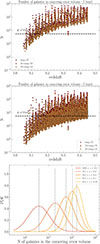 |
Fig. 9. Top: Number of galaxies in the comoving error volume of BNS detected by ET alone (top panel) and in a network with CE (middle panel). Each point corresponds to one GW BNS detection. Different colors correspond to different magnitude intervals. The black dashed line represents the number of WST fibres. Bottom: Probability distribution function of the number of galaxies with apparent I-band magnitude m < 25 that can be found in the comoving error volume of each BNS detected by ET + CE, for different redshift intervals. Dashed vertical lines indicate the mean value around which each Gaussian is centred. |
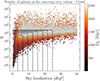 |
Fig. 10. Number of galaxies in the comoving error volume of BNS detected by ET in a network with CE, as a function of their sky localisation. Each point represents one GW BNS detection. The black dashed lines represent an indication of what WST can cover in one night of observations, as described in Sect. 5.1. |
The right balance must be found in the choice of the exposure time to adopt with WST, between long exposures allowing for deeper observations and short exposures allowing for larger regions of the sky to be tiled. Overall, in a stand-alone scenario where WST is used to target galaxies without additional information on EM counterpart candidates from previous photometric observations, shorter (∼30-minute exposures) are preferable. In this framework, the high sensitivity of the IFS can be leveraged to primarily target the peak of the probability distribution within the GW sky localisation and the regions containing extended galaxies.
5.2. Further investigation of size and magnitude of galaxies in the comoving error volume
A galaxy-targeted search is a way to find the EM counterpart from a system gravitationally bounded to its host galaxy. However, there are some feasibility caveats that have to be taken into account, especially for fibre observations concerning the host galaxy sizes, the counterpart brightness, and the counterpart offset from the host galaxy centre.
With the exception of on-axis GRB afterglow detections, which can outshine the host galaxy, the EM counterparts of BNS mergers are typically faint and may be outshined by their host galaxies. Typical magnitudes of galaxies at z < 0.5 (Ilbert et al. 2005), as well as those of the host galaxy of SGRB in the same redshift range reported in the Broad-band Repository for Investigating Gamma-ray burst Host galaxies Traits (BRIGHT, Fong et al. 2022; Nugent et al. 2022) catalogue are brighter than the distribution of the median magnitude of KN and GRB afterglows, following ET BNS. However, these counterparts are not expected to be found at small offsets from their host centre, as also supported by the measured SGRB projected physical offsets. The median value of SGRB offsets is of 1.5 re (where re is the effective radius of the host galaxy; Fong et al. 2022), with more than 60% of those at z < 0.5 lying at > 1re. Considering the host galaxy profiles of the SGRB at z < 0.5 presented in the Fong & Berger (2013) sample, the host galaxy surface brightness at the offsets of the SGRB would be comparable or much fainter than those expected for KN detectable by WST. In such cases, the possibility of identifying the KN spectrum overimposed on the host galaxy one would not be compromised.
However, this situation implies that more fibres should be used for each targeted galaxy in order to cover regions as large as the suitable projected offsets. We refer to this type of fibres displaced in a group configuration as a ‘fibre bundle’. This configuration is not currently included in the WST baseline but is under active consideration within the WST consortium. We emphasise that it would be extremely valuable for this multi-messenger science case. In Fig. 11, we show the distribution of the SGRB offsets from Fong et al. (2022), Nugent et al. (2022) for SGRB at z < 0.5 and some representative fibre bundles, so that we can cover offsets up to ∼5″.
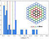 |
Fig. 11. Distribution of the offsets of SGRBs at z < 0.5 from the sample presented in Fong et al. (2022). The dashed colored lines represent the angular size that could potentially be covered by an example fibre bundle configuration, as shown in the sketch in the upper right corner. |
The cases where the EM counterpart explosion site would fall in the same fibre as the host galaxy centre would be especially difficult. This would require a spectral subtraction of the host spectrum, which would ideally have been obtained with WST previously, thanks to the WST survey. We note that the spectral subtraction can also be performed after the transient has faded, by acquiring the host galaxy spectrum within a few weeks of the event. While this approach would not allow for detailed spectroscopic follow-up of the transient itself, it would still enable kilonova detection and redshift measurements for the host. This would have an impact on other science cases, such as the determination of H0. Of course, we note that the galaxies in the regions covered by IFS observations are less affected by these issues.
5.3. The WST golden cases
From Figs. 5 and 9 we can define the golden cases for the WST stand-alone scenario. Up to a redshift of z ∼ 0.3, 0.2 for the ET + CE and ET alone configurations, respectively, it is possible to achieve sky localisations of the GW sources corresponding to a number of galaxies within the comoving error volume of BNS detections that can be easily covered with a few hours of WST observations. This is illustrated in Fig. 12 showing that, at Ω < 10deg2, 3 one-hour WST exposures would cover the relevant number of galaxies for the vast majority of the events (left panel of Fig. 12). For the events with Ω < 1deg2 (right panel of Fig. 12), we find that one exposure is sufficient for almost all the events. By taking into account the use of fibre bundles, the same results are valid up to redshift z ∼ 0.2, 0.1, for the ET + CE and ET alone configurations, respectively, when considering bundles of 20 fibres. The events at z < 0.3 (0.2) with a sky localisation < 10deg2 would be more than 5000 (2000) over the whole sky within 10 years of observations with ET + CE and more than 100 with ET alone.
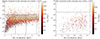 |
Fig. 12. Number of galaxies in the comoving error volume of ET + CE BNS at z < 0.3 with Ω < 10deg2 (left) and Ω < 1deg2 (right). The black dashed lines represent an indication of the potential coverage of WST with three (left panel) and single (right panel) 1 hour exposures, as described in Sect. 5.1. |
We stress that even for the events with small sky localisation regions, the comoving error volume can be large (see Fig. C.8) and the role of WST multiplexing remains crucial for targeting the large number of galaxies within it. As highlighted by Loffredo et al., significant improvements in sky localisation can also be achieved when the ET operates as part of a network with present-day detectors, LIGO, Virgo, KAGRA, and LIGO-India at their design sensitivities. Within a redshift of 0.2, the number of events localised within 10 square degrees is comparable to that obtained when ET is in a network with CE.
5.4. Synergy with optical-NIR photometric observations
The WST can also work in synergy with wide-field optical-NIR photometric facilities such as Rubin, assuming that it will be operational after the end of LSST. We note that up to z ∼ 0.2, almost all KN that are detectable with Rubin are also detectable with both WST IFS and fibres (see Fig. 4). In this framework, Rubin could systematically point to the error regions of BNS detected by ET, performing deep observations and promptly identifying EM counterpart candidates. A substantial number of such candidates is expected to be distributed across the broad 2D localisation regions and spectroscopic data are the key to robustly identify and characterise the true counterpart.
Based on extrapolations from the Zwicky Transient Facility2 (ZTF) results, an average of around 200 new transients per deg2 per night from a single Rubin scan is expected (Julien Peloton, priv. comm.). This estimate refers to transient sources detected in a single visit, without any prior detection history, including objects that might later be classified as known phenomena, such as supernovae (SNe) or tidal disruption events (TDEs) via subsequent observations of the same area.
In case of Rubin observations following a BNS detection, WST could target the transients detected by Rubin, by performing ToO observations to using just a fraction of the total number of fibres. Given the estimated density of ∼200 photometrically detected transients per deg2, approximately 600 fibres would be needed per pointing, considering WST FoV of ∼3.1deg2. This would enable the rapid spectroscopic follow-up necessary for transient identification, while preserving the remaining fibre resources for other science cases.
In this scenario, the IFS would be advantageous for covering the high-density regions of newly discovered transients, coupled with the high-probability areas of the GW signal, and possibly the regions where more extended galaxies are located as well. We note that current transient rate estimates remain highly uncertain. However, the start of LSST operations at Rubin, expected before the end of 2025, will significantly improve our ability to constrain these rates and better inform future observing strategies.
6. Summary and conclusions
In this work, we explore the potential of IFS and MOS capabilities of the WST for the detection, identification, and characterisation of EM counterparts to BNS detected by next-generation GW interferometers. To this end, we used simulations of BNS merger populations, incorporating different neutron star equations of state and mass distributions. We simulated the corresponding GW signals considering both the Δ and 2L ET designs, both for ET alone and in a network with CE. For each detected merger, we assigned a KN light curve based on AT2017gfo (gfo-like KN sample) or numerical relativity-informed models (theoretical KN sample). We also included simulations of GRB afterglow emission.
Rough spectra were constructed from the fit of the simulated photometric data and processed using WST ETC to compute the S/N in both WST IFS and MOS modes. Simulations show that WST can detect KNe up to redshift z ∼ 0.4 and magnitudes mAB ∼ 25. GRB afterglows will primarily contribute for on-axis and slightly off-axis events, up to a viewing angle Θview ∼ 15°, and can be detected up to higher redshifts (beyond z = 1).
In this paper, we discuss two main observing strategies: one with WST in a stand-alone scenario and the other in synergy with large FoV, sensitive photometric facilities, such as Rubin. In this latter case, WST observations will likely use only a fraction of WST fibres, enabling simultaneous WST survey observations. Alternatively, in a stand-alone scenario, with WST, approximately 30 000 fibres and the IFS can be employed in a galaxy-targeted strategy, covering the large number of galaxies in the wide GW error volumes. Improving the completeness of galaxy catalogues with redshift information at z ≤ 0.5 will be essential for optimizing this strategy. This will directly enable targeted observations of galaxies at redshifts consistent with the GW signal’s error volume.
In our analysis, we consider the spatial offset between the EM counterparts and the centre of their host galaxies, as well as their respective brightness. We find that in most cases the EM counterparts will not lie beyond the effective radius of their host galaxies and that the host galaxy surface brightness at the offsets of the EM counterpart would be comparable to or much fainter than the counterpart itself. Mini-IFUs with fibre bundles would be a solution to detect sources with large offsets from the host galaxy centre and allow for the coverage of extended galaxies at low redshift. Based on current offset distributions of KNe and SGRBs from their host centres, not using fibre bundles would likely result in detecting KNe in less than half of the cases. In some cases, the EM counterpart and its host galaxy may appear as superposed point sources. In such scenarios, spectral subtraction using previously acquired host galaxy spectra would be necessary. The acquisition of galaxy spectra up to z ∼ 0.5 as part of WST survey would be a great advantage for effectively performing this kind of subtraction.
Throughout this study, we limited our analysis to ET BNS with sky localisation uncertainties smaller than 100 deg2 (40 deg2 for ET in a network with CE). Even with these constraints, the expected number of events remains substantial, necessitating the development of additional prioritization criteria for optical follow-up. Such criteria should first rely on information extracted from the GW signal, such as the luminosity distance, to exclude events that are too distant to be detected and/or the inclination angle.
We identified a subset of ‘golden’ events for WST follow-up that are at redshifts z < 0.3 and that have sky localisations better than 10 deg2. These events are ideal because they allow for WST to cover all the galaxies in the error volume with a limited number of exposures. We estimated them to be from ∼10 (ET-alone configuration) to hundreds per year (ET + CE configuration). WST contribution is particularly valuable also for well-localised events, because uncertainties in luminosity distance (even at low redshift) can still produce large 3D error volumes containing numerous galaxies to target.
Regardless of whether WST operates in a stand-alone mode or in synergy with other observatories, we find that ToO observations for the research of KNe can begin within 12–24 hours after the GW detection. This changes if GRB prompt gamma-ray emission is detected by high-energy satellites at the same time of GW detection, suggesting an on-axis configuration. In such cases, WST becomes particularly valuable if the GRB localisation is coarse (∼arcminutes): the IFS can be efficiently used to scan the region, refine the position, and promptly identify the EM counterpart. Timely follow-up observations are especially critical for GRB afterglows, which follow rapidly decaying power-law light curves, with observations starting within a few hours after the GRB prompt detection.
In conclusion, the development of the future large FoV, high-sensitivity, IFS, and high-multiplexing facilities should go beyond the more traditional science cases of galaxy survey and stellar population studies. The need to handle the combination of necessary depths, large sky regions, and vast numbers of objects to be targeted makes them a powerful tool in addressing the challenges of the research of EM counterparts of next-generation GW-detected BNS mergers. No existing MOS or IFS facility currently has the sensitivity and multiplexing capabilities required to fully address the BNS multi-messenger science case. The observational strategies are complex. They must be planned well in advance of operations and take full advantage of the information available from the GW signal. Furthermore, to make the best scientific exploitation, such multi-messenger observations not only require the capability to react to alerts with ToO observations, but also the ability to perform a quasi-real-time quick data reduction and analysis so as to alert the community of the EM counterpart detection as soon as possible. This would enable a swift activation of the most appropriate space- and ground-based facilities to perform deeper single-object observations to characterize the evolution of the EM counterpart and its properties. It is clear that the multi-messenger science of the future will need new instruments where this science case is included from the early phases of their development, thereby shaping their specifications and requirements.
Acknowledgments
The authors aknowledge Albino Perego, Andrew J. Levan, Daniele Bjorn Malesani, Jan Harms and Julien Peloton for helpful discussion. S.B. acknowledges support from the Erasmus+ programme. S.B. and S.D.V. acknowledge support by the API Gravitational waves and compact objects of Paris Observatory and by the Programme National des Hautes Energies (PNHE) of CNRS/INSU co-funded by CNRS/IN2P3, CNRS/INP, CEA and CNES. E.L. acknowledges funding by the European Union – NextGenerationEU RFF M4C2 1.1 PRIN 2022 project 2022RJLWHN URKA. M.B. and E.L. acknowledge financial support from the Italian Ministry of University and Research (MUR) for the PRIN grant METE under contract no. 2020KB33TP. U.D. acknowledges Stefano Bagnasco, Federica Legger, Sara Vallero, and the INFN Computing Center of Turin for providing support and computational resources. R.I.A. is funded by the Swiss National Science Foundation through an Eccellenza Professorial Fellowship (award PCEFP2_194638). The authors aknowledge the Astrophysics Centre for Multi-messenger studies in Europe (ACME) funded under the European Union’s Horizon Europe Research and Innovation programme under Grant Agreement No 101131928. The authors aknowledge the Wide-field Spectroscopic Telescope collaboration and the Research Group Ondes Gravitationnelles.
References
- Abac, A., Abramo, R., Albanesi, S., et al. 2025, ArXiv e-prints [arXiv:2503.12263] [Google Scholar]
- Abbott, B. P., Abbott, R., Abbott, T. D., et al. 2017a, ApJ, 848, L12 [Google Scholar]
- Abbott, B. P., Abbott, R., Abbott, T. D., et al. 2017b, Phys. Rev. Lett., 119, 161101 [Google Scholar]
- Abbott, B. P., Abbott, R., Abbott, T. D., et al. 2017c, ApJ, 848, L13 [CrossRef] [Google Scholar]
- Abbott, B. P., Abbott, R., Abbott, T. D., et al. 2017d, Nature, 551, 85 [Google Scholar]
- Abbott, B. P., Abbott, R., Abbott, T. D., et al. 2020a, Liv. Rev. Relat., 23, 3 [NASA ADS] [Google Scholar]
- Abbott, B. P., Abbott, R., Abbott, T. D., et al. 2020b, ApJ, 892, L3 [NASA ADS] [CrossRef] [Google Scholar]
- Abbott, R., Abbott, T. D., Acernese, F., et al. 2023a, Phys. Rev. X, 13, 011048 [NASA ADS] [Google Scholar]
- Abbott, R., Abbott, T. D., Acernese, F., et al. 2023b, Phys. Rev. X, 13, 041039 [Google Scholar]
- Akmal, A., Pandharipande, V. R., & Ravenhall, D. G. 1998, Phys. Rev. C, 58, 1804 [Google Scholar]
- Andreoni, I., Margutti, R., Banovetz, J., et al. 2024, ArXiv e-prints [arXiv:2411.04793] [Google Scholar]
- Antoniadis, J., Freire, P. C. C., Wex, N., et al. 2013, Science, 340, 448 [Google Scholar]
- Bacon, R., Maineiri, V., Randich, S., et al. 2024, ArXiv e-prints [arXiv:2405.12518] [Google Scholar]
- Baym, G., Pethick, C., & Sutherland, P. 1971, ApJ, 170, 299 [NASA ADS] [CrossRef] [Google Scholar]
- Berger, E. 2014, ARA&A, 52, 43 [CrossRef] [Google Scholar]
- Bianco, F. B., Drout, M. R., Graham, M. L., et al. 2019, PASP, 131, 068002 [Google Scholar]
- Bombaci, I., & Logoteta, D. 2018, A&A, 609, A128 [EDP Sciences] [Google Scholar]
- Branchesi, M., Maggiore, M., Alonso, D., et al. 2023, JCAP, 2023, 068 [CrossRef] [Google Scholar]
- Bulla, M., Coughlin, M. W., Dhawan, S., & Dietrich, T. 2022, Universe, 8, 289 [NASA ADS] [CrossRef] [Google Scholar]
- Colombo, A., Sharan Salafia, O., Ghirlanda, G., et al. 2025, A&A, 704, A260 [NASA ADS] [CrossRef] [EDP Sciences] [Google Scholar]
- Coulter, D. A., Foley, R. J., Kilpatrick, C. D., et al. 2017, Science, 358, 1556 [NASA ADS] [CrossRef] [Google Scholar]
- D’Avanzo, P. 2015, J. High Energy Astrophys., 7, 73 [CrossRef] [Google Scholar]
- D’Avanzo, P., Campana, S., Salafia, O. S., et al. 2018, A&A, 613, L1 [NASA ADS] [CrossRef] [EDP Sciences] [Google Scholar]
- de Jong, R. S., Agertz, O., Berbel, A. A., et al. 2019, Messenger, 175, 3 [Google Scholar]
- Douchin, F., & Haensel, P. 2001, A&A, 380, 151 [NASA ADS] [CrossRef] [EDP Sciences] [Google Scholar]
- Dupletsa, U., Harms, J., Banerjee, B., et al. 2023, Astron. Comput., 42, 100671 [NASA ADS] [CrossRef] [Google Scholar]
- Fong, W., & Berger, E. 2013, ApJ, 776, 18 [NASA ADS] [CrossRef] [Google Scholar]
- Fong, W.-F., Nugent, A. E., Dong, Y., et al. 2022, ApJ, 940, 56 [NASA ADS] [CrossRef] [Google Scholar]
- Frohmaier, C., Vincenzi, M., Sullivan, M., et al. 2025, ApJ, 992, 158 [Google Scholar]
- Ghirlanda, G., Salafia, O. S., Pescalli, A., et al. 2016, A&A, 594, A84 [NASA ADS] [CrossRef] [EDP Sciences] [Google Scholar]
- Ghirlanda, G., Salafia, O. S., Paragi, Z., et al. 2019, Science, 363, 968 [NASA ADS] [CrossRef] [Google Scholar]
- Gillanders, J. H., Smartt, S. J., Sim, S. A., Bauswein, A., & Goriely, S. 2022, MNRAS, 515, 631 [NASA ADS] [CrossRef] [Google Scholar]
- Goldstein, A., Veres, P., Burns, E., et al. 2017, ApJ, 848, L14 [CrossRef] [Google Scholar]
- Guidorzi, C., Margutti, R., Brout, D., et al. 2017, ApJ, 851, L36 [NASA ADS] [CrossRef] [Google Scholar]
- Hogg, D. W. 1999, ArXiv e-prints [arXiv:astro-ph/9905116] [Google Scholar]
- Hotokezaka, K., Nakar, E., Gottlieb, O., et al. 2019, Nat. Astron., 3, 940 [NASA ADS] [CrossRef] [Google Scholar]
- Ilbert, O., Tresse, L., Zucca, E., et al. 2005, A&A, 439, 863 [NASA ADS] [CrossRef] [EDP Sciences] [Google Scholar]
- Iorio, G., Mapelli, M., Costa, G., et al. 2023, MNRAS, 524, 426 [NASA ADS] [CrossRef] [Google Scholar]
- Jin, S., Trager, S. C., Dalton, G. B., et al. 2024, MNRAS, 530, 2688 [NASA ADS] [CrossRef] [Google Scholar]
- Kann, D. A., Klose, S., Zhang, B., et al. 2011, ApJ, 734, 96 [NASA ADS] [CrossRef] [Google Scholar]
- Kasen, D., Metzger, B., Barnes, J., Quataert, E., & Ramirez-Ruiz, E. 2017, Nature, 551, 80 [Google Scholar]
- Kiziltan, B., Kottas, A., De Yoreo, M., & Thorsett, S. E. 2013, ApJ, 778, 66 [NASA ADS] [CrossRef] [Google Scholar]
- Lamb, G. P., Lyman, J. D., Levan, A. J., et al. 2019, ApJ, 870, L15 [NASA ADS] [CrossRef] [Google Scholar]
- Lattimer, J. M., & Steiner, A. W. 2014, ApJ, 784, 123 [Google Scholar]
- Lazzati, D., Deich, A., Morsony, B. J., & Workman, J. C. 2017, MNRAS, 471, 1652 [NASA ADS] [CrossRef] [Google Scholar]
- Levan, A. J., Gompertz, B. P., Salafia, O. S., et al. 2024, Nature, 626, 737 [NASA ADS] [CrossRef] [Google Scholar]
- Lipunov, V. M., Gorbovskoy, E., Kornilov, V. G., et al. 2017, ApJ, 850, L1 [NASA ADS] [CrossRef] [Google Scholar]
- Loffredo, E., Hazra, N., Dupletsa, U., et al. 2025, A&A, 697, A36 [NASA ADS] [CrossRef] [EDP Sciences] [Google Scholar]
- Logoteta, D., Perego, A., & Bombaci, I. 2021, A&A, 646, A55 [NASA ADS] [CrossRef] [EDP Sciences] [Google Scholar]
- Mainieri, V., Anderson, R. I., Brinchmann, J., et al. 2024, ArXiv e-prints [arXiv:2403.05398] [Google Scholar]
- Margutti, R., Cowperthwaite, P., Doctor, Z., et al. 2018, ArXiv e-prints [arXiv:1812.04051] [Google Scholar]
- Mooley, K. P., Deller, A. T., Gottlieb, O., et al. 2018, Nature, 561, 355 [Google Scholar]
- Mooley, K. P., Anderson, J., & Lu, W. 2022, Nature, 610, 273 [NASA ADS] [CrossRef] [Google Scholar]
- Nicholl, M., Berger, E., Kasen, D., et al. 2017, ApJ, 848, L18 [NASA ADS] [CrossRef] [Google Scholar]
- Nugent, A. E., Fong, W.-F., Dong, Y., et al. 2022, ApJ, 940, 57 [NASA ADS] [CrossRef] [Google Scholar]
- Oertel, M., Hempel, M., Klähn, T., & Typel, S. 2017, Rev. Mod. Phys., 89, 015007 [Google Scholar]
- Özel, F., & Freire, P. 2016, ARA&A, 54, 401 [Google Scholar]
- Özel, F., Psaltis, D., Narayan, R., & Santos Villarreal, A. 2012, ApJ, 757, 55 [Google Scholar]
- Perego, A., Radice, D., & Bernuzzi, S. 2017, ApJ, 850, L37 [NASA ADS] [CrossRef] [Google Scholar]
- Perego, A., Logoteta, D., Radice, D., et al. 2022, Phys. Rev. Lett., 129, 032701 [NASA ADS] [CrossRef] [Google Scholar]
- Pian, E., D’Avanzo, P., Benetti, S., et al. 2017, Nature, 551, 67 [Google Scholar]
- Planck Collaboration VI. 2020, A&A, 641, A6 [NASA ADS] [CrossRef] [EDP Sciences] [Google Scholar]
- Punturo, M., Abernathy, M., Acernese, F., et al. 2010, CQG, 27, 194002 [NASA ADS] [CrossRef] [Google Scholar]
- Rastinejad, J. C., Gompertz, B. P., Levan, A. J., et al. 2022, Nature, 612, 223 [NASA ADS] [CrossRef] [Google Scholar]
- Reitze, D., Adhikari, R. X., Ballmer, S., et al. 2019, BAAS, 51, 35 [NASA ADS] [Google Scholar]
- Ricigliano, G., Perego, A., Borhanian, S., et al. 2024, MNRAS, 529, 647 [NASA ADS] [CrossRef] [Google Scholar]
- Ronchini, S., Branchesi, M., Oganesyan, G., et al. 2022, A&A, 665, A97 [NASA ADS] [CrossRef] [EDP Sciences] [Google Scholar]
- Ryan, G., van Eerten, H., Piro, L., & Troja, E. 2020, ApJ, 896, 166 [CrossRef] [Google Scholar]
- Salafia, O. S., & Ghirlanda, G. 2022, Galaxies, 10, 93 [NASA ADS] [CrossRef] [Google Scholar]
- Santoliquido, F., Mapelli, M., Giacobbo, N., Bouffanais, Y., & Artale, M. C. 2021, MNRAS, 502, 4877 [NASA ADS] [CrossRef] [Google Scholar]
- Savchenko, V., Ferrigno, C., Kuulkers, E., et al. 2017, ApJ, 848, L15 [NASA ADS] [CrossRef] [Google Scholar]
- Schechter, P. 1976, ApJ, 203, 297 [Google Scholar]
- Smartt, S. J., Chen, T. W., Jerkstrand, A., et al. 2017, Nature, 551, 75 [NASA ADS] [CrossRef] [Google Scholar]
- Soares-Santos, M., Holz, D. E., Annis, J., et al. 2017, ApJ, 848, L16 [CrossRef] [Google Scholar]
- Tanaka, M., Kato, D., Gaigalas, G., & Kawaguchi, K. 2020, MNRAS, 496, 1369 [NASA ADS] [CrossRef] [Google Scholar]
- Tanvir, N. R., Levan, A. J., González-Fernández, C., et al. 2017, ApJ, 848, L27 [CrossRef] [Google Scholar]
- Troja, E., Piro, L., Ryan, G., et al. 2018, MNRAS, 478, L18 [NASA ADS] [CrossRef] [Google Scholar]
- Valenti, S., Sand, D. J., Yang, S., et al. 2017, ApJ, 848, L24 [CrossRef] [Google Scholar]
- Villar, V. A., Guillochon, J., Berger, E., et al. 2017, ApJ, 851, L21 [Google Scholar]
Appendix A: Additional information on the simulated datasets
Appendix A.1: KN modelling of set 1 (gfo-like)
The modelling of AT2017gfo-like KN emission adopts the best-fit parameters from column BFc of Table 1 in Perego et al. (2017). The model comprises three anisotropic ejecta components - dynamical, wind, and secular - each defined by mass m, polar angle θ distribution, root-mean-square (rms) radial speed v, and angle-dependent grey opacity k. The dynamical ejecta has mass mdyn = 0.005 M⊙, distributed as sin2(θ), velocity vdyn = 0.23c, and opacity kdyn = 1cm2g−1 for θ < π/6, increasing to 30cm2g−1 otherwise. The wind ejecta extends to θ < π/3, with mass mw = 0.15mdisc, where mdisc = 0.1 M⊙ is the disc mass; the velocity is vw = 0.067c, and the opacity kw is set to 1 cm2g−1 for θ ≤ π/6, and to 5 cm2g−1 for π/6 < θ ≤ π/3. The secular ejecta has mass ms = 0.20mdisc, velocity vs = 0.04c, and uniform opacity ks = 5cm2g−1 at all latitudes.
Appendix A.2: Correction of the blue band for set 1
The limitations of the black-body approximation in modelling KN emission become evident in the UV band (Gillanders et al. 2022). KN ejecta, which are rich in heavy elements, exhibit strong line blanketing in the UV due to blue photons being absorbed in the opaque ejecta and re-emitted at redder wavelengths. The black-body approximation fails to capture this effect. Moreover, our KN modelling, based on Perego et al. (2017) and Branchesi et al. (2023), assumes grey opacities, thereby neglecting spatial and temporal variations in opacity. This leads to an overestimation of the blue component in the spectrum. In Fig. A.1 we present synthetic spectral continuum of AT2017gfo, computed from the light curve model in Perego et al. (2017) used to construct set 1 (see Sect. 2.1). A luminosity distance of 40 Mpc and a viewing angle of θview = 25° were imposed, consistent with Table 1 in Perego et al. (2017). By comparing Fig. A.1 with AT2017gfo data (e.g. Pian et al. (2017)), it is evident that the synthetic spectra lack the pronounced spectral bump between approximately 4000Å and 5000Å observed in AT2017gfo. This discrepancy is primarily due to an overestimation of the blue component. Moreover, the bump in the synthetic spectrum emerges around 2 days, while the bump of AT2017gfo is at ∼1.44 days, suggesting a ±0.5 day uncertainty in our model’s bump timing.
To mitigate the overestimation of the UV component in our spectra, we devise a correction informed by the findings of Gillanders et al. (2022). Their work used radiative transfer simulations to reproduce the spectra of AT2017gfo during photospheric emission, examining various ejecta compositions and classifying them based on the average electron fraction (Ye). In their Figs. 5 and 6, Gillanders et al. compare the observed 1.4-day spectrum of AT2017gfo with model predictions for different Ye values, along with a continuum spectrum. This continuum, calculated at the same temperature as the best-fit model (Ye = 0.37) but without accounting for ejecta composition, relies on the black-body approximation and, like our model, overpredicts the UV emission.
We extract fluxes corresponding to the continuum and various Ye values (Ye = 0.37a, 0.44a, 0.05b) from Figs. 5 and 6 of Gillanders et al. (2022), denoting them as fλ, c and fλ, Ye, respectively. The continuum and Ye = 0.37a fluxes are represented by the orange and blue lines in Fig. 5, while the Ye = 0.44a and Ye = 0.05b fluxes correspond to the blue and purple lines in Fig. 6, respectively. The difference between the black-body approximation and the radiative transfer simulations is expected to be influenced by the opacity of the ejecta (Tanaka et al. 2020). To quantify this discrepancy in the 3000 Å ≲λ≲ 5000 Å region, we compute the following ratio for each Ye:
 (A.1)
(A.1)
where Ic and IYe are the integrals of the continuum and Ye fluxes over λ, then we have
 (A.2)
(A.2)
We set λmin = 3000 Å. The upper bound λmax depends on Ye: for lanthanide-poor ejecta (Ye > 0.3), we use λmax = 4250 Å, while for lanthanide-rich ejecta (Ye ≤ 0.3), we use λmax = 5000 Å. Figure A.2 shows the computed ratio R as a function of Ye (black crosses). We observe a linear correlation between R and Ye, and a linear fit yields:
 (A.3)
(A.3)
where A = 0.2857 and B = 0.3658, as indicated by the grey dashed line in Fig. A.2. The ratio R serves as a correction factor for adjusting the KN fluxes from Branchesi et al. (2023).
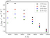 |
Fig. A.1. AT2017gfo-like KN fλ in Rubin filters as function of wavelength (observer frame), computed at four different time instants, assuming luminosity distance of 40 Mpc and viewing angle 25°, in agreement with the value reported in column BFc of Table 1 from Perego et al. 2017 for AT2017gfo. |
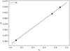 |
Fig. A.2. Ratio of flux integrals R = Ic/IYe as defined in Eq. A.1, calculated using the fluxes extracted from Figs. 5 and 6 of Gillanders et al. 2022. These fluxes correspond to the continuum (orange line in Fig. 5), Ye = 0.37a (blue line in Fig. 5), Ye = 0.44a (blue line in Fig. 6), and Ye = 0.05b (purple line in Fig. 6). The dashed grey line represents the linear fit as detailed in Eq. A.3. |
To implement the correction to the KN fluxes, we first evaluate the KN flux, fλs(ts), in the source frame, where λs and ts represent the emission wavelength and time, respectively. For times between 0.5 and 3 days, when the emission is primarily dominated by the dynamical ejecta, we use the dynamical opacity kdyn to infer the corresponding electron fraction Ye, based on Table 1 of Tanaka et al. (2020). In our model of AT2017gfo-like spectra, kdyn varies with the polar viewing angle (Perego et al. 2017). For viewing angles θv < π/6, we assume kdyn = 1 cm · g−1, yielding Ye = 0.4; for larger angles, we use kdyn = 30 cm · g−1, corresponding to Ye = 0.1.
For ts ≥ 3 days, when the emission is dominated by the secular ejecta, we adopt a secular opacity of ks = 5 cm · g−1, from which we infer Ye = 0.31, again using Table 1 of Tanaka et al. (2020).
Once the appropriate value of Ye has been determined, we compute the correction factor R using Eq. A.3 and apply it to the flux in the source frame. The corrected flux is given by
 (A.4)
(A.4)
We apply this correction up to λs = 4250 Å for Ye > 0.3, and λs = 5000 Å otherwise.
In Fig. A.3, we show the synthetic spectrum computed before and after applying the correction of Eq. A.4 for an AT2017gfo-like event, located at the luminosity distance of 40 Mpc and observed with a 25° viewing angle. Comparing our synthetic spectrum both before and after applying the correction with AT2017gfo data, for example Fig. 4 of Villar et al. (2017), we find that the emission in the u filter (3694 Å) is excessively high before applying the correction (approximately 19 magnitudes two days after the merger), but aligns more closely with the AT2017gfo observation after the correction (approximately 20 magnitudes two days after the merger).
Our method for generating KN spectral continuum is an approximation, mainly because of the limited frequency range, the employment of grey opacities, and the assumption of black-body emission. Even with these limitations, our estimated population of KN spectral curves remains valuable, serving as a critical tool in calibrating the features of next-generation spectroscopic telescopes and evaluating their performance.
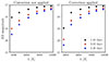 |
Fig. A.3. Our observer frame spectrum of an AT2017gfo-like KN, computed at three distinct time points with an assumed luminosity distance of 40 Mpc and a viewing angle of 25 degrees. The left panel displays the spectrum before applying any correction, while the right panel illustrates the spectrum after applying the flux correction as detailed in Eq. A.4. A comparison with the AT2017gfo observational data, see for example Villar et al. 2017, reveals that the u filter emission (3694 Å) is initially too high. After implementing the correction, the emission aligns more closely with the observational data. |
Appendix A.3: Choice of the EoS for sets 2 and 3
Although both EoSs are consistent with current astrophysical constraints on tidal deformability (from GW170817), as well as on the maximum NS mass and radius (Antoniadis et al. 2013; Lattimer & Steiner 2014; Oertel et al. 2017), they bracket current uncertainties in NS compactness. While predicting similar maximum NS masses, APR4 yields significantly more compact NSs than BLh, leading to systematically smaller ejecta masses, and thus dimmer, faster-fading KN emission, compared to BLh. The two EOSs also differ in the behaviour of the nuclear incompressibility K, which characterises the pressure response of nuclear matter to changes in baryon density. Perego et al. 2022 showed that the value of K at the maximum Tolman– Oppenheimer–Volkoff (TOV) baryon density, together with the maximum TOV mass, influences the mass threshold for prompt collapse to a BH for BNS with arbitrary mass ratios. In our modelling, this leads APR4 to consistently predict lower threshold masses for prompt collapse than BLh, resulting in smaller ejecta masses and fainter, faster-fading KN light curves. We refer the reader to Loffredo et al. (2025) for technical details.
Appendix B: Exposure time
We present in this appendix the same plots reported in Sect. 4, but considering this time 1800s exposures instead of 3600 s ones.
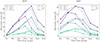
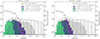
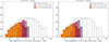
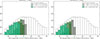
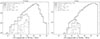
Appendix C: Additional plots
In this appendix we provide supplementary figures related to our analysis. The first set of figures(C.1 to C.4) present the same distributions shown in Sect. 4, but for the WST IFS rather than MOS. Figure C.1 shows the detectability of KNe as a function of time using WST IFS. Figure C.2 displays the i-band magnitude distribution of WST IFS-detectable KNe at 12 hours post-merger, while Fig. C.3 shows the g-band magnitude distribution of WST-detectable KNe for both IFS and MOS modes. Finally, Fig. C.4 illustrates the redshift distribution of WST IFS-detectable KNe at 12 hours post-merger. These figures complement the main text by providing a detailed view of WST IFS performance.
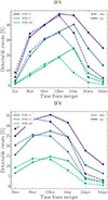 |
Fig. C.1. Percentage of gfo-like KNe (top) and theoretical KNe (bottom) following BNS mergers detected by ET in the 2L configuration that are detectable with WST IFS. Different colors indicate different S/Ns; dashed and solid lines correspond to the blue and red arms of the spectrographs, respectively. The highest detectability occurs approximately 12–24 hours post-merger. |
Figure C.5 shows the magnitude distribution of WST-detectable KNe in Rubing and i filters from 12 to 48 hours post-merger, highlighting how KNe become fainter in the g band relative to the i band at later epochs.
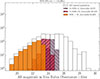 |
Fig. C.2. Magnitude distribution in i filter of ET BNS detected over 10 years and their corresponding theoretical KN at ∼ 12 hours after the merger. The background distribution in white corresponds to the parent BNS+KN population. The colored distributions correspond to the EM counterparts that are detectable with WST IFS red arm, different colors corresponding to different S/N intervals. |
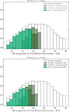 |
Fig. C.3. Magnitude distribution in g filter of ET BNS and corresponding theoretical KN at ∼ 12 hours after the merger. The background distribution in white corresponds to the parent BNS+KN population. The colored distributions correspond to the EM counterparts that are detectable with WST IFS (top panel) and MOS (bottom panel) blue arm, different colors corresponding to different S/N intervals. EM counterparts detectable with Rubin are shown in grey. |
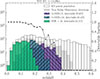 |
Fig. C.4. Redshift distribution of ET BNS detected over 10 years and the corresponding theoretical KN at ∼ 12 hours after the merger. The background distribution in white corresponds to the parent BNS+KN population. The colored distributions correspond to the EM counterparts that are detectable with WST IFS blue or red arm, different colors corresponding to different S/N intervals. EM counterparts detectable with Rubin are shown in grey. Black points refer to the y axis ticks on the right hand side and show the fraction of detectable (S/N > 3) EM counterparts, with no additional information on the S/N range, with respect to Rubin detections. |
Figure C.6 illustrates the contribution of GRB afterglows to WST detections as a function of viewing angle and redshift. While the contribution extends to high redshift (z > 1), it is primarily limited to on-axis and slightly off-axis systems. This trend is further emphasized in Fig. C.7, which shows the viewing angle distribution of WST IFS-detectable events at different times post-merger, separated into two cases: events where the KN outshines the afterglow, predominantly corresponding to off-axis systems, and events where the afterglow dominates over the KN, mainly associated with on-axis or slightly off-axis systems.
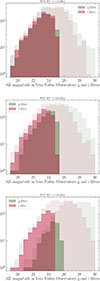 |
Fig. C.5. Magnitude distribution in i and g filters of KNe that are detectable with WST at ∼ 12 (left), 24 (centre) and 48 (right) hours post-merger. The background histograms show the BNS+KN parent population. |
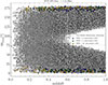 |
Fig. C.6. Viewing angle as a function of redshift of GRB afterglows following BNS mergers (white points) detected by ET in a network with CE. Colored points represent WST detections, different colors corresponding to different S/N. Percentages are given with respect to the number of Rubin detections. |
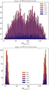 |
Fig. C.7. Viewing angle distribution of the population of events featuring an afterglow, that are detectable with WST IFS red arm, both when the afterglow outshines the KN (bottom) panel and viceversa (top). Different colors refer to different times post-merger. The GW interferometers network includes ET and CE. |
The final set of figures relates to Sect. 5.1, where the galaxy-targeted search is discussed. Figure C.8 shows the distribution of ΔDL and sky localisation regions for ET+CE BNS, illustrating how these quantities increase with luminosity distance and can produce large error volumes even at low redshift. Figure C.9 presents separate plots of the ΔDL and sky localisation distributions for different luminosity distance intervals.
Figure C.10 is similar to Fig. 10, but color-coded by BNS viewing angle. It highlights how on-axis events yield less precise luminosity distance estimates, resulting in larger error volumes that contain a substantial number of galaxies, even when the sky localisation is relatively small.
Figure C.11 shows the same analysis presented in Sect. 5.1 for ET+CE BNS (Fig. 10), this time considering ET-only BNS. It is evident that only a small fraction of ET BNS have all galaxies in the error volume observable with WST within a single night.
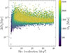 |
Fig. C.8. Uncertainty on the GW luminosity distance as a function of sky localisation for each BNS detected by ET in a network with CE, at z < 0.45. The color of the points is related to the luminosity distance DL of the events as reported in the lateral color bar. |
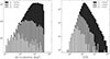 |
Fig. C.9. Distribution of sky localisation (left panel) and uncertainty on DL (right panel) for different values of DL of BNS detected by ET in a network with CE. |
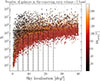 |
Fig. C.10. Number of galaxies in the comoving error volume of BNS at z < 0.45 detected by ET in a network with CE, as a function of their sky localisation. Vertical dashed lines represent the sky area covered for increasing number of exposures. Horizontal dashed lines refer to the corresponding number of WST fibers available within the FoV considered. The color bar refers to the viewing angle Θview. |
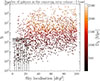 |
Fig. C.11. Number of galaxies in the comoving error volume of BNS at z < 0.45 detected by ET alone, as a function of their sky localisation. Vertical dashed lines represent the sky area covered for increasing number of exposures. Horizontal dashed lines refer to the corresponding number of WST fibers available within the FoV considered. The color bar refers to the GW signal luminosity distance. |
Appendix D: Comparison with current multiplexing facilities
To stress the potential impact of WST relative to current MOS facilities, we estimate the capabilities of the latter in detecting and identifying EM counterparts of BNS mergers observable by ET and CE, using the observing strategies explored in this work. We take as reference the low-resolution spectrographs (LRS) of 4MOST (de Jong et al. 2019) and WEAVE (Jin et al. 2024), which are mounted on 4 m-class telescopes (ESO/VISTA and WHT respectively) and represent current cutting-edge MOS instruments.
The first relevant parameter is the limiting magnitude. These facilities can reach i-band limiting magnitudes of ∼203 in one-hour exposures under observing conditions similar to those assumed in this work, achieving an S/N per Å of ∼10. This magnitude range limits the detectable KN population to events within z ≲ 0.05–0.1 (see Fig. 1). For reference, this limiting magnitude is also shown together with the i-band magnitude distribution of WST-detectable KNe in Fig. 3.
In terms of multiplexing, the 4MOST LRS deploys 1624 fibres (812+812) over a 4.2 deg2 FoV, while WEAVE deploys ∼950 fibres over a ∼3.1 deg2 field. If we consider a galaxy-targeted search with the same assumptions as in Sect. 5.1, but focusing on ET (+ CE) BNS at z < 0.1 and conservatively selecting only galaxies with mAB < 21, we find that, for the majority of the events, tens (a few) exposures would be required to cover all such galaxies within the error volume of this close BNS subpopulation, using the full fibre complement. The fibre apertures are 1.45 arcsec for 4MOST and 1.3 arcsec for WEAVE. WEAVE additionally offers 20 integral-field units (mini-IFUs) of 37 fibres each, whereas 4MOST LRS does not plan fibre bundles; this makes it more challenging to capture offset KNe, which are expected to constitute a significant fraction of the population (See Sect. 5.2).
If these facilities are used in synergy with deep photometric surveys, for example LSST as outlined in the Time Domain Extragalactic Survey (TiDES; Frohmaier et al. 2025), only the brightest events would be targetable in one-hour exposures, and only a fraction of the available fibres would be used for such follow-up. Furthermore, dedicated, real-time telescope-level ToO observations are not envisioned for either facility, making it difficult to apply the tiling strategies discussed in this work.
In summary, current MOS facilities can be useful for detecting and identifying the brightest events at z < 0.1, but will sample only the brightest end of the KN population from ET and CE BNS. Those facilities could be suitable for LVK BNS follow-up. In particular WEAVE mini-IFUs can be especially useful to capture offset KNe and to test the strategy for such configuration in WST optic.
All Tables
Percentage of afterglows outshining KNe in different bins of a viewing angle, Θview, at different times post-merger.
All Figures
|
Fig. 1. AB magnitude in Rubini filter at ∼12 hours post-merger as a function of redshift for KNe and on-axis (θview < 15°) GRB afterglows following BNS detected by ET as a stand-alone observatory (left panels) and in a network with CE (right panels). The few bright KNe (mAB < 21) in the upper-right panel are not visible due to their low density relative to the bulk of the population, which dominates the color scale. The cross, upwards pointing triangle, and star respectively represent AT2017gfo, and the optical counterparts of GRB 211211A (Rastinejad et al. 2022) and GRB 230307A (Levan et al. 2024), two GRBs followed by a KN, at ∼12 hours after the GRB prompt detection. A Gaussian filter was applied to the data in the top panels and bottom-right one for visualisation purposes. |
| In the text | |
|
Fig. 2. Percentage of gfo-like KNe (left) and theoretical KNe (right) following BNS mergers detected by ET in the 2L configuration that are detectable with WST MOS. Different colors indicate different S/Ns; dashed, dotted, and solid lines correspond to the blue, orange, and red arms of the spectrographs, respectively. The highest detectability occurs approximately 12–24 hours post-merger. The peak time of the detectability reflects the optimal observational window across the full range of ejecta masses, compositions, and inclinations considered in our simulations. |
| In the text | |
|
Fig. 3. Magnitude distribution in i filter of ET BNS detected over 10 years and their corresponding theoretical KN at ∼12 hours after the merger. The background distribution in white corresponds to the parent BNS + KN population. The colored distributions correspond to the EM counterparts that are detectable with the WST MOS red arm, with different colors corresponding to different S/N intervals. The dashed vertical line indicates the approximate magnitude limit of current MOS facilities, such as 4MOST and WEAVE, for a one-hour exposure. |
| In the text | |
|
Fig. 4. Redshift distribution of ET BNS detected over 10 years and the corresponding theoretical KN at ∼12 hours after the merger. The background distribution in white corresponds to the parent BNS + KN population. The colored distributions correspond to the EM counterparts that are detectable with WST MOS blue or orange or red arm, different colors corresponding to different S/N intervals. EM counterparts detectable with Rubin are shown in grey. Black points refer to the y axis ticks on the right hand side and show the fraction of detectable (S/N > 3) EM counterparts, with no additional information on the S/N range, with respect to Rubin detections. |
| In the text | |
|
Fig. 5. Sky localisation uncertainty as a function of redshift of BNS (white points) detected with ET (left panel) and ET + CE (right panel) over 10 years. Grey points refer to the EM counterparts detectable with Rubin, among which the colored points refer to those that are detectable with WST IFS blue arm at ∼12 hours post-merger. Different colors correspond to different S/N. Percentage reported in the legend refer to the fraction of EM counterparts that are detectable with WST, with respect to those that are detectable with Rubin. The black dashed line represents WST patrol area, 3.1 deg2, where fibres will be positioned. |
| In the text | |
|
Fig. 6. Viewing angle as a function of redshift of theoretical KN following BNS mergers (white points) detected by ET alone (top panel) and ET in a network with CE (bottom panel). Colored points represent WST detections, different colors corresponding to different S/N. The lack in GW detections for edge-on systems is due to GW signal S/N, that is higher for face-on systems with respect to edge-on systems with the same intrinsic parameters. |
| In the text | |
|
Fig. 7. Magnitude distribution in the Rubini filter (with a cut at m = 30) of afterglows produced by BNS mergers with a viewing angle below 15° (solid black line), at ∼12 hours (top panel) and ∼3 days (bottom panel) post-merger. Dashed- and dot-line black histograms correspond to events that are detectable with WST (i.e. where the combined flux of the afterglow and KN has S/N > 3) and for which the afterglow outshines the KN, for Θview < 10° and 10° < Θview < 15°, respectively. Dashed- and dot-line gray histograms represent detectable events where the kilonova dominates over the afterglow, for Θview < 10° and 10° < Θview < 15°, respectively. |
| In the text | |
|
Fig. 8. Comoving error volume as a function of GW luminosity distance for each BNS detected by ET in a network with CE at z < 0.45. The color of the points refers to the uncertainty on the sky localisation, according to the color bar on the right. |
| In the text | |
|
Fig. 9. Top: Number of galaxies in the comoving error volume of BNS detected by ET alone (top panel) and in a network with CE (middle panel). Each point corresponds to one GW BNS detection. Different colors correspond to different magnitude intervals. The black dashed line represents the number of WST fibres. Bottom: Probability distribution function of the number of galaxies with apparent I-band magnitude m < 25 that can be found in the comoving error volume of each BNS detected by ET + CE, for different redshift intervals. Dashed vertical lines indicate the mean value around which each Gaussian is centred. |
| In the text | |
|
Fig. 10. Number of galaxies in the comoving error volume of BNS detected by ET in a network with CE, as a function of their sky localisation. Each point represents one GW BNS detection. The black dashed lines represent an indication of what WST can cover in one night of observations, as described in Sect. 5.1. |
| In the text | |
|
Fig. 11. Distribution of the offsets of SGRBs at z < 0.5 from the sample presented in Fong et al. (2022). The dashed colored lines represent the angular size that could potentially be covered by an example fibre bundle configuration, as shown in the sketch in the upper right corner. |
| In the text | |
|
Fig. 12. Number of galaxies in the comoving error volume of ET + CE BNS at z < 0.3 with Ω < 10deg2 (left) and Ω < 1deg2 (right). The black dashed lines represent an indication of the potential coverage of WST with three (left panel) and single (right panel) 1 hour exposures, as described in Sect. 5.1. |
| In the text | |
|
Fig. A.1. AT2017gfo-like KN fλ in Rubin filters as function of wavelength (observer frame), computed at four different time instants, assuming luminosity distance of 40 Mpc and viewing angle 25°, in agreement with the value reported in column BFc of Table 1 from Perego et al. 2017 for AT2017gfo. |
| In the text | |
|
Fig. A.2. Ratio of flux integrals R = Ic/IYe as defined in Eq. A.1, calculated using the fluxes extracted from Figs. 5 and 6 of Gillanders et al. 2022. These fluxes correspond to the continuum (orange line in Fig. 5), Ye = 0.37a (blue line in Fig. 5), Ye = 0.44a (blue line in Fig. 6), and Ye = 0.05b (purple line in Fig. 6). The dashed grey line represents the linear fit as detailed in Eq. A.3. |
| In the text | |
|
Fig. A.3. Our observer frame spectrum of an AT2017gfo-like KN, computed at three distinct time points with an assumed luminosity distance of 40 Mpc and a viewing angle of 25 degrees. The left panel displays the spectrum before applying any correction, while the right panel illustrates the spectrum after applying the flux correction as detailed in Eq. A.4. A comparison with the AT2017gfo observational data, see for example Villar et al. 2017, reveals that the u filter emission (3694 Å) is initially too high. After implementing the correction, the emission aligns more closely with the observational data. |
| In the text | |
|
Fig. C.1. Percentage of gfo-like KNe (top) and theoretical KNe (bottom) following BNS mergers detected by ET in the 2L configuration that are detectable with WST IFS. Different colors indicate different S/Ns; dashed and solid lines correspond to the blue and red arms of the spectrographs, respectively. The highest detectability occurs approximately 12–24 hours post-merger. |
| In the text | |
|
Fig. C.2. Magnitude distribution in i filter of ET BNS detected over 10 years and their corresponding theoretical KN at ∼ 12 hours after the merger. The background distribution in white corresponds to the parent BNS+KN population. The colored distributions correspond to the EM counterparts that are detectable with WST IFS red arm, different colors corresponding to different S/N intervals. |
| In the text | |
|
Fig. C.3. Magnitude distribution in g filter of ET BNS and corresponding theoretical KN at ∼ 12 hours after the merger. The background distribution in white corresponds to the parent BNS+KN population. The colored distributions correspond to the EM counterparts that are detectable with WST IFS (top panel) and MOS (bottom panel) blue arm, different colors corresponding to different S/N intervals. EM counterparts detectable with Rubin are shown in grey. |
| In the text | |
|
Fig. C.4. Redshift distribution of ET BNS detected over 10 years and the corresponding theoretical KN at ∼ 12 hours after the merger. The background distribution in white corresponds to the parent BNS+KN population. The colored distributions correspond to the EM counterparts that are detectable with WST IFS blue or red arm, different colors corresponding to different S/N intervals. EM counterparts detectable with Rubin are shown in grey. Black points refer to the y axis ticks on the right hand side and show the fraction of detectable (S/N > 3) EM counterparts, with no additional information on the S/N range, with respect to Rubin detections. |
| In the text | |
|
Fig. C.5. Magnitude distribution in i and g filters of KNe that are detectable with WST at ∼ 12 (left), 24 (centre) and 48 (right) hours post-merger. The background histograms show the BNS+KN parent population. |
| In the text | |
|
Fig. C.6. Viewing angle as a function of redshift of GRB afterglows following BNS mergers (white points) detected by ET in a network with CE. Colored points represent WST detections, different colors corresponding to different S/N. Percentages are given with respect to the number of Rubin detections. |
| In the text | |
|
Fig. C.7. Viewing angle distribution of the population of events featuring an afterglow, that are detectable with WST IFS red arm, both when the afterglow outshines the KN (bottom) panel and viceversa (top). Different colors refer to different times post-merger. The GW interferometers network includes ET and CE. |
| In the text | |
|
Fig. C.8. Uncertainty on the GW luminosity distance as a function of sky localisation for each BNS detected by ET in a network with CE, at z < 0.45. The color of the points is related to the luminosity distance DL of the events as reported in the lateral color bar. |
| In the text | |
|
Fig. C.9. Distribution of sky localisation (left panel) and uncertainty on DL (right panel) for different values of DL of BNS detected by ET in a network with CE. |
| In the text | |
|
Fig. C.10. Number of galaxies in the comoving error volume of BNS at z < 0.45 detected by ET in a network with CE, as a function of their sky localisation. Vertical dashed lines represent the sky area covered for increasing number of exposures. Horizontal dashed lines refer to the corresponding number of WST fibers available within the FoV considered. The color bar refers to the viewing angle Θview. |
| In the text | |
|
Fig. C.11. Number of galaxies in the comoving error volume of BNS at z < 0.45 detected by ET alone, as a function of their sky localisation. Vertical dashed lines represent the sky area covered for increasing number of exposures. Horizontal dashed lines refer to the corresponding number of WST fibers available within the FoV considered. The color bar refers to the GW signal luminosity distance. |
| In the text | |
Current usage metrics show cumulative count of Article Views (full-text article views including HTML views, PDF and ePub downloads, according to the available data) and Abstracts Views on Vision4Press platform.
Data correspond to usage on the plateform after 2015. The current usage metrics is available 48-96 hours after online publication and is updated daily on week days.
Initial download of the metrics may take a while.