| Issue |
A&A
Volume 705, January 2026
|
|
|---|---|---|
| Article Number | A79 | |
| Number of page(s) | 16 | |
| Section | Galactic structure, stellar clusters and populations | |
| DOI | https://doi.org/10.1051/0004-6361/202556268 | |
| Published online | 07 January 2026 | |
Centrally concentrated star formation in young clusters
1
Department of Astronomy, Columbia University,
538 W 120th St.,
New York,
NY
10027,
USA
2
Department of Astrophysics, American Museum of Natural History,
200 Central Park W.,
New York,
NY
10024,
USA
3
Gumarbek Daukeyev Almaty University of Power Engineering and Telecommunications,
126/1 Baytursynuli St.,
Almaty
050000,
Kazakhstan
4
Heriot-Watt University Aktobe Campus, K. Zhubanov Aktobe Regional University,
263 Zhubanov Brothers St.,
Aktobe
030000,
Kazakhstan
5
Physics Department, Nazarbayev University,
53 Kabanbay Batyr Ave.,
Astana
010000,
Kazakhstan
6
Energetic Cosmos Laboratory, Nazarbayev University,
53 Kabanbay Batyr Ave.,
Astana
010000,
Kazakhstan
7
Max Planck Institute for Astrophysics,
Karl-Schwarzschild-Straße 1,
85748
Garching bei München,
Germany
8
Department of Physics and Astronomy, McMaster University,
1280 Main St. W.,
Hamilton,
ON
L8S 4M1,
Canada
9
Department of Physics, Drexel University,
3141 Chestnut St.,
Philadelphia,
PA
19104,
USA
10
Fesenkov Astrophysical Institute,
23 Observatory St.,
050020
Almaty,
Kazakhstan
11
Al-Farabi Kazakh National University,
71 Al-Farabi ave.,
050040
Almaty,
Kazakhstan
★ Corresponding author: This email address is being protected from spambots. You need JavaScript enabled to view it.
Received:
4
July
2025
Accepted:
10
November
2025
Abstract
The study of star cluster evolution necessitates modeling how their density profiles develop from their natal gas distribution. Observational evidence indicates that many star clusters follow a Plummer-like density profile. However, most studies have focused on the phase after gas ejection, neglecting the influence of gas on early dynamical evolution. We investigate the development of star clusters forming within gas clouds, particularly those with a centrally concentrated gas profile. Simulations were conducted using the Torch framework, integrating the FLASH magnetohydrodynamics code into AMUSE. This permitted detailed modeling of star formation, stellar evolution, stellar dynamics, radiative transfer, and gas magnetohydrodynamics. We study the collapse of centrally concentrated, turbulent spheres with a total mass of 2.5 × 10³ M⊙, investigating the effects of varying numerical resolution and star formation scenarios. The free-fall time is shorter at the center than at the edges of the cloud, with a minimum value of 0.55 Myr. The key conclusions from this study are: (1) the final stellar density profile is more centrally concentrated than was analytically predicted, reflecting the role of global gas collapse and feedback; (2) subclusters can initially form even in centrally concentrated gas clouds; (3) gas collapses globally toward the center on the central free-fall timescale, contradicting the assumption in analytical models of local fragmentation and star formation; and (4) the mass of the most massive star formed is directly correlated with the cluster effective radius and inversely correlated with the velocity dispersion, while the duration of star formation correlates with the star formation efficiency.
Key words: magnetohydrodynamics (MHD) / stars: formation / open clusters and associations: general
© The Authors 2026
 Open Access article, published by EDP Sciences, under the terms of the Creative Commons Attribution License (https://creativecommons.org/licenses/by/4.0), which permits unrestricted use, distribution, and reproduction in any medium, provided the original work is properly cited.
This article is published in open access under the Subscribe to Open model. This email address is being protected from spambots. You need JavaScript enabled to view it. to support open access publication.
1 Introduction
Stars form within molecular clouds (MCs), in regions where gas accumulates under the influence of self-gravity (Lada & Lada 2003). Due to the critical role of this process, the formation of star clusters from MCs has been extensively studied via observations (Burki 1978; O’Connell 2004; Kuhn et al. 2015; Motte et al. 2022; Schroetter et al. 2025) and simulations (Lada et al. 1984; Goodwin 1997; Goodwin & Bastian 2006; Baumgardt & Kroupa 2007; Chen & Ko 2009; Pelupessy & Portegies Zwart 2012; Grudić et al. 2018; Shukirgaliyev et al. 2019b; Lewis et al. 2023; Polak et al. 2024). The formation and early evolution of star clusters involve not only the accumulation of gas but also the emergence of filamentary structures (Elmegreen & Scalo 2004; Canning et al. 2014; Alina et al. 2019; Rhea et al. 2025), as well as the influence of stellar feedback mechanisms, including stellar winds (Agertz et al. 2013; Dale et al. 2014; Fierlinger et al. 2016; Härer et al. 2025), radiation pressure (Sales et al. 2014; Rahner et al. 2019; Kim et al. 2018; Dale et al. 2025), and supernova explosions (Hopkins et al. 2012; Rogers & Pittard 2013). Observations of associated gas suggest that the upper limit of the cluster formation timescale is around 10 Myr (e.g., Leisawitz et al. 1989). Emerging clusters are often identified through the detection of H II regions (Heydari-Malayeri et al. 2003; Gusev et al. 2016; Komesh et al. 2024).
While many stars form within embedded clusters, not all clusters survive their early evolution or remain gravitationally bound over long timescales. Observational studies indicate that a significant fraction of clusters disperse within 10-20 Myr, with fewer than 4-7% of those initially embedded in MCs surviving the gas expulsion phase to remain bound (Lada & Lada 2003; Baumgardt & Kroupa 2007). However, clusters with a star formation efficiency (SFE) of 15-20% or higher exhibit a greater probability of long-term survival (Goodwin 1997; Smith et al. 2011; Shukirgaliyev et al. 2017). More recent studies suggest that, under specific initial conditions, clusters may remain bound with SFEs as low as 3-5% (Shukirgaliyev et al. 2021).
Whether a cluster remains bound may be due to the density profile of the MC from which it formed. Chen et al. (2021) suggest that rotating massive clusters, such as globular clusters, originate from centrally concentrated clouds in the early Universe. In particular, globular clusters, especially older and more massive ones, are known to exhibit strong central stellar concentrations (O’Dell 2001). This structure is often well described by the Plummer (1911) profile. Such centrally concentrated stellar profiles are also found in dense young clusters. For example, the Orion Nebula Cluster shows a stellar distribution within the central 0.5 pc that closely matches this profile (Stutz 2018). Beyond the Plummer radius, a, the shape of the cluster appears to be influenced by the surrounding gas filament, illustrating the interplay between the gas morphology and stellar dynamics during early cluster evolution.
Li et al. (2019) used the AREPO hydrodynamics code (Springel 2010) to show that the evolution of MCs, driven by turbulent gas motions, leads to the formation of complex filamentary structures. Turbulent flows compress the gas under the influence of gravity, causing local collapse at filament intersections, where dense clumps form. This hub-filament structure leads to star formation (Myers 2009; Zhang et al. 2024a,b). The resulting stellar subclusters often merge to form a larger stellar cluster. As stellar feedback increases, the surrounding gas either dissipates or collapses further, enhancing the filamentary structure. A subsequent study using AREPO showed that a gas cloud with a sufficiently centrally concentrated profile forms a single massive star cluster at its center, which then begins to accrete gas from the surrounding region (Chen et al. 2021). This accretion-driven formation results in compact central clusters.
The initial gas density profile and the resulting stellar distribution after gas expulsion are critical determinants of cluster survival. Adams (2000) showed that a centrally concentrated stellar distribution substantially increases the likelihood of survival after gas removal. Building on this, Parmentier & Pfalzner (2013) developed a semi-analytical model in which the stellar density profile is steeper than the initial or residual gas profile. In their model, star formation proceeds through local gravitational collapse within the gas clump, with a constant star formation efficiency per free-fall time, εff, while the gas density profile remains fixed over the duration of star formation, tSF. These assumptions naturally produce centrally concentrated stellar configurations, enhancing the long-term gravitational boundedness of the cluster.
Shukirgaliyev et al. (2017) tested the model of Parmentier & Pfalzner (2013) by fitting the post-expulsion stellar distribution to a Plummer (1911) profile at different SFEs. Their approach assumed instantaneous gas expulsion and focused on whether the resulting stellar systems could remain gravitationally bound. They demonstrated that clusters can survive with a global SFE as low as 15%, lowering the critical threshold from the previously suggested 20-30% range (Baumgardt & Kroupa 2007; Smith et al. 2011; Brinkmann et al. 2017). They argued that survival under such extreme, rapid gas-loss conditions implies an even greater likelihood of survival in more gradual, physically realistic scenarios. When evolved, their model clusters closely resemble observed open clusters in the solar neighborhood (Kalambay et al. 2022; Bissekenov et al. 2024a; Ishchenko et al. 2025; Kalambay et al. 2025; Weis et al. 2025).
Gas dynamics significantly affect early cluster evolution. Proszkow & Adams (2009) and Shukirgaliyev et al. (2017) showed that a higher SFE at the moment of gas expulsion leads to a larger fraction of stars remaining gravitationally bound. Additionally, Smith et al. (2011) argued that the local stellar fraction within the half-mass radius is a more accurate predictor of cluster survivability than the global SFE. Gas removal alters the gravitational potential, often resulting in the expansion of the surviving clusters by a factor of 3-4 (Baumgardt & Kroupa 2007). Fall et al. (2010) further showed that the SFE is closely linked to the surface density of protoclusters, highlighting the need to accurately model gas dynamics during formation.
Several recent studies, such as those by Farias et al. (2019) and Farias & Tan (2023), have explored the effects of gradual star formation and gas dispersal using simplified hydrodynamic approaches within turbulent clumps. While these efforts provide valuable insight into the broader evolutionary trends of embedded clusters, our study extends their work by employing a state-of-the-art star formation framework that self-consistently couples gas dynamics, stellar feedback, and gravitational evolution at high resolution.
In our work, we extend the Shukirgaliyev et al. (2017) model by beginning with pure gas and evolving the system during the star formation phase “prior” to gas expulsion, incorporating the dynamical impact of directly modeled gas. We aim to quantify how the evolving gas density influences the cluster’s stellar distribution.
We use the Torch framework (Wall et al. 2019, 2020), which combines magnetohydrodynamics (MHD) and N-body models within the Astrophysical Multipurpose Software Environment (AMUSE; Pelupessy et al. 2013). Modeling gas dynamics in starforming regions requires accurately capturing turbulence, which plays a critical role in regulating gas fragmentation and collapse (Larson 1981; McKee & Ostriker 2007). Achieving a realistic treatment of turbulent gas structures, particularly the formation of dense clumps that initiate star formation, demands high spatial resolution, but this in turn requires significant computational resources.
Previous studies, such as Cournoyer-Cloutier et al. (2023), have employed the Torch framework to investigate the evolution of stellar clusters at high resolution. However, these simulations assumed a larger initial gas mass and included primordial binaries, which significantly increased computational costs and restricted the exploration of a broader parameter space. Unlike Cournoyer-Cloutier et al. (2023), we do not include primordial binaries and instead adopt a more moderate initial gas mass and a simplified setup to allow systematic exploration across different initial conditions.
In this work, we aim to model star cluster formation under controlled and computationally efficient conditions, while still capturing key aspects of gas dynamics and feedback processes. We study how gas evolution influences the dynamical state and structural properties of stellar clusters formed within centrally concentrated environments. In our initial conditions, we implement the gas profile derived by Shukirgaliyev et al. (2017), enabling us to test whether the simulated clusters develop the expected Plummer-like structure after gas removal.
This paper is organized as follows. In Sect. 2, we describe the numerical methods and initial conditions. Sect. 3 presents the simulation results and discusses our findings in the context of previous studies. The limitations of our models are addressed in Sect. 4. Finally, we summarize our conclusions and outline directions for future work in Sect. 5.
2 Method
We used the Torch framework (Wall et al. 2019, 2020) to simulate the formation of star clusters from gas. In this work, we used Torch version 1.0. Torch uses the AMUSE framework (Portegies Zwart et al. 2009; Pelupessy et al. 2013; Portegies Zwart et al. 2013, 2019), for which we used commit 044ca1f7a. In the version used here, AMUSE connects the MHD code FLASH version 4.6.2 (Fryxell et al. 2000; Dubey et al. 2014), the stellar evolution code SeBa (Portegies Zwart & Verbunt 1996; Toonen et al. 2012), the SmallN code (Hut et al. 1995; Portegies Zwart & McMillan 2018), and the fourth-order Hermite N-body dynamics solver ph4 (McMillan et al. 2012). We used Multiples (Portegies Zwart & McMillan 2018) to regularize close binaries and few-body interactions that arise dynamically during the simulation.
FLASH is an adaptive mesh refinement (AMR) grid code. We chose the HLLD Riemann solver (Miyoshi & Kusano 2005) with reconstruction of the third-order piecewise parabolic method (Colella & Woodward 1984).
2.1 Gravity bridge
We coupled the stellar and gaseous components using a variant of the BRIDGE method (Fujii et al. 2007; Portegies Zwart et al. 2020), which provides a Hamiltonian splitting framework to combine different integration schemes. In this approach, the interaction is advanced with a kick-drift-kick sequence: the stars receive a velocity update from the gravitational field of the gas, evolve under their internal N-body dynamics with ph4, and are then updated again by the gas. The gas undergoes an analogous sequence, receiving accelerations from the stars while being evolved hydrodynamically with FLASH. Although the bridge is formally symplectic, the use of a fourth-order Hermite scheme for stars and a second-order solver for gas introduces additional integration errors; however, these remain small for the timestep sizes considered (Wall et al. 2019). Mutual forces are computed consistently by mapping stellar masses onto the AMR grid with a cloud-in-cell scheme and solving for the potential with the FLASH multigrid method (Ricker 2008), ensuring momentum conservation and symmetry in the coupling.
2.2 Stellar feedback
The simulations include stellar feedback from photoionization, far-ultraviolet (far-UV) radiation pressure, and stellar winds, with sources restricted to stars of M > 7 M⊙. Stars with M ≳ 20 M⊙ dominate feedback through ionizing radiation, winds, and supernovae (Haworth et al. 2018), though more recent studies indicate that feedback effects may already become significant at somewhat lower masses, around M ~ 13 M⊙ (Yan et al. 2023).
Radiation transport was handled with the FERVENT module (Baczynski et al. 2015), which follows the ray-tracing algorithm of Wise & Abel (2011) implemented in ENZO. Ionizing photon luminosities and mean photon energies are determined from stellar masses and ages: for stars with T* > 2.75 × 10⁴ K these values are interpolated from the OSTAR2002 grid (Lanz & Hubeny 2003), while for cooler stars they are estimated from blackbody spectra (Stahler & Palla 2004). Heating from ionization is calculated as the difference between photon energies and the ionization potential of hydrogen. Far-UV photons in the range 5.6-13.6 eV are also included, which are absorbed by dust and eject photoelectrons. For lower-mass massive stars (7 ≲ M/M⊙ ≲ 13), the far-UV luminosity approaches that of ionizing radiation. Dust was restricted to gas cooler than 3 × 10⁶ K to avoid unphysical cooling in regions where the grains would have been destroyed (Draine 2011). Stellar winds were implemented using the momentum injection scheme of Wall et al. (2019, 2020), which is inspired by the inversion of the method described in Simpson et al. (2015). For further details on the feedback implementation, see Wall et al. (2020).
Numerical parameters and resolution settings for simulations.
2.3 Mesh refinement
The computational domain has a side length of 13.75 pc. We employed AMR, with a base grid 163 at level 1, and a minimum refinement level of 2. The maximum refinement level, denoted by n, varies between simulations and takes values from 3 to 6 depending on the specific run. For brevity, we refer to the maximum refinement level as simply the “refinement level” throughout the paper. A detailed summary of the simulation parameters is provided in Sect. 2.6.
The AMR grid was refined based on temperature gradients and the local Jeans (1902) length,
![Mathematical equation: \lambda_j = [\pi c_s^2 / (G \rho)]^{1/2},](/articles/aa/full_html/2026/01/aa56268-25/aa56268-25-eq1.png) (1)
(1)
where cs is sound speed, ρ is the gas density, and G is the gravitational constant. Refinement and derefinement are triggered when the Jeans length falls below 12 cell widths and above 24 cell widths, respectively. The temperature-triggered refinement or derefinement occurs when the adapted Löhner (1987) estimator of temperature gradient exceeds 0.98 or drops below 0.6, respectively.
At refinement level n, the maximum number of cells is given by Cellsmax = 16 × 2n−1. The corresponding minimum cell size ∆xmin can be derived from Cellsmax and is listed in Table 1. The minimum allowed resolution in the lower-density outer regions corresponds to 323 grid cells, yielding a maximum cell size of ∆xmax = 0.429pc.
2.4 Sink properties and star formation
Gas collapses on timescales of the free-fall time,
![Mathematical equation: t_{\rm ff} = [3\pi/ (32 G \rho)]^{1/2}.](/articles/aa/full_html/2026/01/aa56268-25/aa56268-25-eq2.png) (2)
(2)
As the density increases, the free-fall time shortens, accelerating the collapse. This makes it challenging to resolve star formation in simulations due to the diminishing timesteps needed to resolve the collapse. To address this, we collected regions of dense gas into sink particles (Bate et al. 1995; Krumholz et al. 2004) using the method implemented in FLASH by Federrath et al. (2010).
We set the sink threshold density ρsink and accretion radius rsink such that, at the minimum cell size ∆xmin, the Jeans length satisfies λj = 6∆xmin = 2rsink, which represents a modified version of the criterion used in Truelove et al. (1997), consistent with the requirement of Heitsch et al. (2001) that, for high refinement levels, the local Jeans length be resolved by at least six grid cells to ensure adequate magnetohydrodynamic support. When the density exceeds ρsink, and the additional boundedness and convergence criteria outlined in Federrath et al. (2010) are met, a sink particle is formed with all the dense gas within rsink. After formation, the sink particle accretes all mass within its accretion radius that exceeds the threshold density. Mass found within overlapping accretion zones accretes to the sink with the closest center of mass (Wall et al. 2019). On each time step, each sink particle is moved to the center of mass of the stars and gas within its radius of accretion (Cournoyer-Cloutier et al. 2021). Sink particles exert gravitational force on gas, stars, and each other through direct summation. New sink particles cannot be created within the accretion radius of an existing sink, which prevents artificial overlap of sinks (Federrath et al. 2010).
Each sink particle on formation was assigned a list of stellar masses randomly drawn using Poisson sampling (Sormani et al. 2017; Wall et al. 2019), with masses sampled from the Kroupa (2002) initial mass function (IMF), ranging from Mmin = 0.08 M⊙ to Mmax = 150 M⊙. Each sink forms the next star in the list as soon as it accumulates enough mass. Thus, the total mass,
 (3)
(3)
is conserved. Despite formation of primordial binaries being implemented in Torch (Cournoyer-Cloutier et al. 2021), no primordial binaries are initialized in these models. Other work by Cournoyer-Cloutier et al. (2021, 2023, 2024) investigates primordial binaries in detail. In particular, Cournoyer-Cloutier et al. (2023) shows that their presence does not affect the overall cluster structure (e.g., size and shape) while star formation is ongoing. In the following, massive stars are defined as stars with M > 7 M⊙.
2.5 Model setup
We adopted a star cluster model based on the centrally concentrated star formation scenario proposed by Parmentier & Pfalzner (2013), in which star formation occurs locally at all positions within the gas clump with a constant efficiency per local free-fall time. This assumption results in a stellar distribution that forms self-consistently while maintaining a constant total density profile (stars plus gas) throughout the star formation process.
Shukirgaliyev et al. (2017) modified this model by requiring the final stellar distribution, ρ*(r), to follow a Plummer (1911) profile
 (4)
(4)
where M* is the total stellar mass and a* is the Plummer radius. Based on the constraint of the constant total density profile,
 (5)
(5)
they recover the corresponding density profile of the residual (unprocessed) gas, ensuring consistency with the original formulation of Parmentier & Pfalzner (2013). The residual gas density profile ρgas is then given by
 (6)
(6)
where k, K1, and K2 are parameters determined by the constant SFE per free-fall time εff and the star formation duration tSF (see Appendix A for further details). This form ensures consistency between the assumed Plummer distribution for the stellar component and the requirement that the sum of stars and gas reproduces the initial gas density profile throughout the star formation process.
We used the assumed total density ρ0 (Eq. (5)) as the initial gas density profile for our simulations, as is shown in Figure 1. This figure also shows the final gas (Eq. (6)) and stellar (Eq. (4)) density profiles derived by Shukirgaliyev et al. (2017) from their assumption of a final Plummer profile, together with the local free-fall time, tff, of the initial gas distribution. The stellar component then forms self-consistently during the simulation.
The initial free-fall time, tff(r), of the gas distribution provides insight into the early dynamical evolution of the system. As is shown in Figure 1, the free-fall time is shorter in the central regions and increases substantially at larger radii, indicating that the gas in the central core collapses much more rapidly than the gas in the outer regions. The minimum free-fall time in the center is tff = 0.55 Myr. We evolve the system for at least 4.5tff with different resolutions, ensuring that the gas within the half-mass radius fully collapses. The free-fall time at the gas half-mass radius is about 2.39 Myr initially.
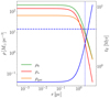 |
Fig. 1 Initial density and free-fall time, teff, of the cluster derived by Shukirgaliyev et al. (2017) as a function of radius. The initial gas density (Eq. (5)) is shown in green, the final stellar density (Eq. (4)) in red, and the final gas density (Eq. (6)) in orange. The initial density profile is used directly in the simulation setup. The free-fall time, tff, of the initial gas density distribution as a function of radius is shown in (solid blue). The horizontal dashed blue line indicates the free-fall time corresponding to the average density, while the vertical dotted blue line marks the half-mass radius, rh, of the initial gas distribution. The local value of tff is shortest in the central regions and increases significantly toward larger radii. |
2.6 Initial conditions
We modeled the collapse of a spherical turbulent gas cloud with a centrally concentrated density profile, embedded in a uniform background medium, and threaded by a weak uniform vertical magnetic field. The cloud has a radius Rsphere = 5.5 pc = 5a*. To choose the cloud density profile, we use an analytic model from Shukirgaliyev et al. (2017) with a stellar mass of M* = 827 M⊙ and 25% SFE, but rescale it to the density profile it had prior to star formation when it was pure gas. This ensures comparability to the structural properties adopted in previous studies (Shukirgaliyev et al. 2017, 2018, 2019b, 2020).
The initial cloud gas mass is Mgas = 2513 M⊙. Our computational box is slightly larger than the spherical cloud of size 5 a* that we initialize. Beyond the cloud ( r > 5.5 pc), we initialize a uniform, initially isothermal background gas at the same temperature Tamb = 20K and density as the surface of the cloud, with zero velocity, to ensure a smooth pressure transition at the boundary and avoid numerical artifacts. For comparison, Shukirgaliyev et al. (2017) measure the global SFE within r < 10a*, as their models exhibit a centrally peaked SFE profile (see Fig. 2 in Shukirgaliyev 2018). Within 10a*, the centrally concentrated stellar profile, which follows approximately ρ* ∝ r−3.3, encloses a total mass (stars + gas) of 3260 M⊙. Truncating the cloud at 5.5 pc and embedding it in this uniform medium increases the total gas mass in the simulation domain to 3597 M⊙, ~10% more than the total mass of gas and stars used in the model by Shukirgaliyev et al. (2017). This approximation has minimal impact on the cloud’s centrally concentrated dynamics. The adopted physical parameters of the cloud are summarized in Table 2.
Within r ≤ Rsphere = 5.5 pc, the cloud is initialized with a turbulent velocity field generated (Wünsch 2015) following a Kolmogorov (1941) velocity spectrum. The surrounding background gas (r > Rsphere) has zero velocity to initialize a static, uniform medium. We set the integrated turbulent virial parameter of the cloud to αvir = 0.5 by setting the cloud’s total turbulent kinetic energy to be half of the total gravitational potential energy. The initial temperature of 20 K defines the thermal internal energy of the gas and the corresponding sound speed, which is independent of the turbulent kinetic energy. Thus, thermal pressure support and turbulent support enter the initial conditions as separate contributions. This approach does not fully balance energies in a centrally concentrated cloud, as higher central density would require stronger turbulent support. However, dissipative processes such as radiative cooling in interstellar clouds prevent sustained virial equilibrium anyway (e.g., Ibáñez-Mejía et al. 2016, 2017; Seifried et al. 2019).We used outflow boundary conditions to allow gas to exit the computational domain, while permitting inflow from boundary regions if the flow was directed inward, preventing unphysical vacuum formation at the edges.
2.7 Models
We performed a series of simulations at different refinement levels to explore the influence of numerical resolution and stochastic IMF sampling on cluster formation. The corresponding numerical parameters for each simulation are listed in Table 1. The refinement level, n, was varied between n = 3 and n = 6, with maximum effective resolutions ranging from 643 to 5123 cells. The minimum cell size, Δxmin, sink accretion radius, rsink, and sink formation threshold, ρsink, were adjusted accordingly to ensure that the local Jeans length was properly resolved. For the lowest-resolution case (n = 3), we conducted ten independent realizations with different random seeds to capture statistical variations resulting from stochastic IMF sampling. The simulation naming convention is nXsY, where X denotes the refinement level and Y specifies the random seed.
Initial physical parameters adopted in the simulations.
3 Results
We now examine what our numerical results reveal about the ultimate structure of the star clusters formed in our simulations.
3.1 Cluster structure
We here compare the density profiles and morphologies of our clusters with the analytically predicted, spherically symmetric, Plummer density profile, ρ*(r), described by Equation (4), with a Plummer radius of a* = 1.1 pc and a total stellar mass of M* = 780 M⊙ (see Fig. 1). We also compare our simulated stellar density profiles with the more general Elson-Fall-Freeman (EFF) profile (Elson et al. 1987), which the Plummer profile is a special case of. Finally, we compare our results with observational data to evaluate their consistency with observed star cluster properties.
The three-dimensional EFF density distribution is given by (Karam & Sills 2022)
 (7)
(7)
where ρ0 is the central density, aeff is the scale radius, and γeff determines the outer slope of the density profile. The Plummer profile corresponds to the special case γeff = 4, while the EFF form allows γeff to vary. We therefore fit both a Plummer profile, with Plummer mass Mpl and scale radius apl as free parameters, and an EFF profile, with ρ0, aeff, and γeff as free parameters, to the simulated stellar distributions to test whether the clusters are consistent with the analytically predicted Plummer profile.
The stellar density profiles of simulated clusters were constructed by binning stellar positions in 20 logarithmically spaced radial shells between the minimum and maximum stellar radii. In each shell, the mean density
 (8)
(8)
where the sum extends over all stars with radii ri ≤ rj < ri+1. Empty bins were excluded from the analysis. The cluster center was determined iteratively by recalculating the mass-weighted centroid while the enclosing radius was reduced by 10% at each step, until fewer than 32 stars remain. This shrinking-sphere procedure yields a robust definition of the cluster center while naturally converging toward the densest subcluster (see e.g., Shukirgaliyev et al. 2017, 2019a,b; Ussipov et al. 2024; Bissekenov et al. 2024a,b, 2025; Ishchenko et al. 2025).
Figure 2 presents the stellar density profiles of the simulated clusters (blue points) at 4tff. The cluster is centered on the densest region, and only the stars within the radius enclosing 95% of the total stellar mass are used for the calculation of the density profile. We compare them with the analytically predicted Plummer profile (dashed orange line) for stellar clusters (shown in Figure 1 and given by Eq. (4)), as well as with the bestfit Plummer (dashed green line) and EFF (dash-dotted magenta line) profiles. The fits are obtained with the curve_fit routine from scipy (Virtanen et al. 2020), which applies the Levenberg-Marquardt algorithm (Levenberg 1944) for nonlinear least squares optimization. To avoid artificial central peaks caused by a few massive stars, the innermost region (0.01-0.2pc, depending on the simulation) was excluded from the fits, and only stars within the radius enclosing 95% of the total stellar mass are used.
This comparison highlights the differences between the evolved stellar systems and the predicted analytic distribution and shows how the Plummer and EFF models capture the structural properties of the clusters. The fitted Plummer and EFF scale radii provide a quantitative measure of the cluster compactness. Some simulations agree well with a Plummer profile (e.g., n3s1, n3s3, n5s1, and n6s1), while others deviate, as indicated by the slope of the density tail in the EFF profile. Nevertheless, the overall structure is reasonably well described by both profiles. With increasing refinement level, the stellar density profiles become smoother and more centrally concentrated, as reflected by the higher densities within 0.1 pc (e.g., comparing n3s1, n4s1, n5s1, and n6s1). Although the analytically predicted Plummer radius is a* = 1.1 pc, the fitted scale radii are systematically smaller, both in apl and in aeff. This shows that the star clusters formed in our models are more compact than predicted. Thus, a centrally concentrated gas distribution under realistic conditions leads to the formation of a more compact stellar cluster than predicted by the analytic model, which assumed local gravitational collapse.
In model n3s3, the snapshot marked by a * is shown 40 kyr earlier than 4tff, because a very massive star of 60 M⊙ forms shortly after this time. At the displayed epoch, however, the dominant feedback arises from an 18 M⊙ star, which controls the gas evolution at that stage. In model n3s7, a 70 M⊙ star forms and the system develops a clear subcluster structure, which prevents meaningful Plummer or EFF fitting. We also note that models n3s6 and n4s1 form subclusters. In cases of subclusters, the profiles are centered on the densest subcluster, so the outer regions may not be fitted correctly.
This conclusion aligns with observations of young clusters such as the Orion Nebula Cluster (ONC). Stutz (2018) derived the stellar mass distribution in the Orion Nebula Cluster primarily from Spitzer-identified YSOs (Megeath et al. 2016), augmented with COUP X-ray data in regions of high nebulosity (Feigelson et al. 2005). They found that the central cluster core (<0.7 pc) contains ~1000-1300 M⊙, surrounded by a more diffuse halo extending to ~2 pc (see their Fig. 4). The inner structure is well fit by a Plummer model with a*~0.36 pc.
3.2 Subcluster formation
Figure 3 shows the stellar distribution and gas density evolution for simulations n3s6, n3s7, and n4s1, which were chosen because they form multiple stellar subclusters. In all cases, the formation of two distinct subclusters is clearly observed. In simulation n4s1, the dynamical interaction between these subclusters becomes particularly evident: initially, the two subclusters form in close proximity and exhibit elongated structures (top row), subsequently merge into a single system (middle row), and later separate again into two subclusters (bottom row). In contrast, in n3s6 and n3s7, the first subcluster forms early around the first massive star (top row), and stellar feedback then disperses the surrounding gas and shifts the dense region spatially (middle row), enabling the later formation of a second subcluster in the displaced gas (bottom row).
These results demonstrate that even in initially centrally concentrated gas clouds, multiple subclusters can emerge depending on the timing and location of massive star formation. This extends the results of Cournoyer-Cloutier et al. (2023) and Polak et al. (2024), who found similar behavior in less centrally concentrated initial gas distributions.
Notably, the formation of multiple stellar subclusters is relatively uncommon in our study: only 3 out of 13 simulations (spanning various refinement levels and random seeds) exhibit clear subcluster formation driven by massive star feedback, whereas the majority evolve into single, merged systems sustained by prolonged central accretion. We identify two distinct pathways for subcluster formation in centrally concentrated clouds: (1) the sequential formation of a secondary stellar subcluster triggered by the displacement of dense gas regions due to feedback from an early massive star, as observed in simulations n3s6 and n3s7; and (2) the near-simultaneous formation of two stellar subclusters in close proximity n4s1. In this case, feedback from massive stars disperses the gas, which reduces the system’s binding energy and halts global collapse. As a result, when the subcluster fall toward the center, they become kinematically dominant and then separate again. This highlights the complex interplay between stellar dynamics, gas accretion, and feedback processes.
At refinement levels n = 4, 5, and 6, two star clusters form at the location of the peak density during the initial stages of the collapse. At n = 5 and n = 6, this occurs at time 1.5 tff (see Fig. 4), and at n = 4, about ~ 200 kyr later. In the cases with n = 5 and 6, the clusters merge (second column), forming a larger cluster that continues to accrete gas toward the center. In contrast, at n = 4, the star clusters first merge and then split again into two clusters. This is probably due to the stronger feedback at n = 4, which is more intense than at higher refinement levels due to the formation of a more massive star. We conclude that star clusters can merge if gas continues accreting at the center for more than a dynamical time and the surrounding gas potential supports the merging process. These results are consistent with the simulation findings reported by Karam & Sills (2024). In summary, our analysis shows that different random initial conditions can lead to variations in the timing and location of massive star formation, sometimes leading to the formation of multiple stellar subclusters.
3.3 Impact of massive stars
In this subsection, we investigate the impact of the most massive stars on SFE and cluster structure. We quantify stellar feedback by measuring the expelled gas mass, Mloss,fb, and examine the dependence of SFE on the duration of star formation, tsf.
In order to examine how stellar feedback depends on the mass of the most massive stars, we focus on the impact of the first massive star that forms with M > 15 M⊙, and examine how it influenced the SFE after 1 Myr. To do this, we chose four simulations with the same resolution, but different random seeds resulting in different maximum stellar masses. We ensured that within the 1 Myr interval between subsequent simulation outputs no more than one massive star was formed. (The one exception is model n3s1, where two massive stars with M > 15 M⊙ appeared; however, this does not contradict our analysis, as this case represents the highest stellar mass considered.) In other cases, where more than one massive star (with M > 15 M⊙) formed within this interval, disentangling their individual contributions would have made the analysis considerably more difficult.
Figure 5 presents snapshots of the gas density and stellar distribution for these four simulations, which are, in order of maximum stellar mass, n3s3, n3s9, n3s4, and n3s1. The left panels correspond to the time of formation of the most massive star with M > 15 M⊙ in each simulation, while the right panels show a time 1 Myr later. For comparison, we highlighted the most massive stars with M > 15 M⊙ to include all stars likely to contribute to feedback.
A comparison of the left and right panels in Figure 5 for each simulation shows how the formation of the most massive stars expels gas differently depending on their individual masses, the values of which are shown in the bottom right corner of each panel. Prior to the formation of the most massive stars, the gas generally collapses toward the center, forming a centrally concentrated star cluster with only limited feedback. Once the most massive stars appear, radiative and mechanical feedback begin to strongly regulate further star formation. Both the formation times of the most massive stars and the corresponding total stellar masses at these times differ (see the time and mass of the star cluster in the bottom right corner of each panel in the first column).
We estimated the feedback during the 1 Myr time interval between the left and right panels of Figure 5 using the following approach. It is well established that stellar feedback expels gas and alters the dynamical evolution of young clusters, while stars may continue to form or be dynamically ejected (Baumgardt & Kroupa 2007; Goodwin 2009). To quantify the gas ejection, we defined the feedback-induced gas mass loss, Mloss,fb, as the difference between the gas mass ejected from the grid and the mass of gas converted into stars within 5.5 pc of the cluster center. We also computed the total stellar mass formed during this period.
Figure 6 shows the stellar mass formed and Mloss,fb for the n3s3, n3s9, n3s4, and n3s1 simulations over the same 1 Myr time interval as the density snapshots shown in Figure 5. As we can see, the stellar mass formed decreases as the mass of the most massive star increases, while Mloss,fb increases. These results indicate that the extremely strong feedback from the most massive stars suppresses subsequent star formation. Star formation does not cease immediately after the onset of feedback; rather, it gradually declines depending on the availability of surrounding gas and the strength of the feedback processes.
Figure 7 shows that the maximum stellar mass, Mmax, correlates with two structural measures - the Plummer radius, apl, and the EFF scale radius, aeff - as well as anti-correlating with the stellar velocity dispersion, σv. Both the structural fits and the velocity dispersion were computed using stars within the radius around the densest region of the cluster that encloses 95% of the total stellar mass, to provide a consistent basis of comparison. The point with aeff = 0.0 was excluded from the fitting, as it does not represent a physical value. These correlations indicate that clusters hosting more massive stars are larger and dynamically colder. Similar trends were seen in less centrally concentrated clusters by Lewis et al. (2023). These trends result primarily from the expulsion of gas in the center of the cluster prior to further star formation by feedback from the most massive star, although dynamical mass segregation can also play a role (Polak et al. 2025; Laverde-Villarreal et al. 2025).
We define a duration of star formation, tsf, as the period from the onset of star formation until the gas mass within the halfmass radius drops below 20% of the total stellar mass. Figure 8 shows the relationship between tsf and the SFE in simulations with n = 3. We see that tsf is positively correlated with SFE. Thus, both the duration of formation and the mass of the most massive stars influence the final SFE of the cluster.
The influence of massive stars and their associated feedback on cluster morphology formation is consistent with the findings of Lewis et al. (2023). However, in their study, a massive star is introduced at the very beginning of cluster evolution, whereas in our simulations, massive stars emerge by chance during the simulation. In contrast, for more massive MCs (e.g., Mcloud ~ 106 M⊙), stellar feedback is generally insufficient to counteract the deep gravitational potential of the cloud (Polak et al. 2024).
Taking into account all the results discussed above, we can answer the question we posed of what controls star formation timing and efficiency. As the mass of the most massive stars increases, stellar feedback becomes stronger, resulting in faster gas expulsion and a more dispersed cluster. Conversely, when the most massive stars are less massive, the gas is removed more gradually, and the resulting cluster remains more centrally concentrated. This trend is quantitatively reflected in the fitted Plummer and EFF radii, which both decrease as the mass of the most massive stars decreases. We note, however, that this conclusion applies to low-mass, low-density clouds such as those considered here; in much more massive systems, feedback from massive stars can be insufficient to halt star formation, so the regulation of efficiency proceeds differently (Polak et al. 2024).
This behavior is consistent with the findings of Chen et al. (2021), who also investigated centrally concentrated gas profiles. However, in their study, the initial gas profile is given by ρ(r) ∝ r−2 and they used an initial gas mass of 8 × 10⁵ M⊙, whereas in our simulations, the gas profile is uniform in the center and follows ρ(r) ∝ r−3.3 beyond the Plummer radius (Shukirgaliyev et al. 2021), with an initial gas mass of ≈ 2.5 × 10³ M⊙.
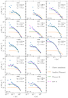 |
Fig. 2 Stellar density profiles at 4tff (blue points) are compared with the analytically predicted Plummer profile for the stellar distribution (dashed orange line), as well as best-fit Plummer (dashed green) and EFF (dash-dotted magenta) models. The mass of the most massive star formed in each simulation is indicated in the lower left corner of each panel. The panel marked with a ★ (n3s3) is shown at a slightly earlier time; see also the text for details on subcluster cases. |
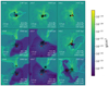 |
Fig. 3 Gas density slices and stellar distribution projections from the n3s6, n3s7, and n4s1 models. In these models subcluster formation occurs. For n3s6 and n3s7: (top row) onset of stellar feedback; (middle row) prior to the formation of the second cluster; (bottom row) after the formation of the second cluster. For n4s1: (top row) two clusters are present; (middle row) clusters merge into a single structure; (bottom row) the system separates again into two clusters. Ionization fronts are indicated by the cyan line. Black dots indicate individual stars, with massive stars shown in red. The symbol size of massive stars is proportional to their mass. Annotations in each panel include: (bottom left) scale bar; (bottom right) mass of the most massive star, total stellar mass within 5.5 pc, and total number of stars; (top left) simulation label; (top right) simulation time. The color scale represents the gas density in grams per cubic centimetre. |
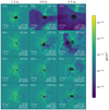 |
Fig. 4 Images of gas density and stellar distribution at different times for different maximum grid resolutions (higher refinement level n corresponds to finer grid resolution). Each row corresponds to a level; each column, to a simulation time (1.5 tff, 3 tff, 4.5 tff). The ionization fronts are marked with cyan lines. Stars are black dots; massive stars are red, with sizes proportional to their masses. In each panel, the notations are as follows: (bottom left) physical scale; (bottom right) the mass of the most massive star, total stellar mass, and number of stars; (top left) model label; (top right) simulation time. The color scale represents the gas density in grams per cubic centimetre. |
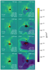 |
Fig. 5 Slices of gas density and projected stellar distribution at the formation time in each model of the most massive star with M > 15 M⊙ (left column), and 1 Myr later (right column), for the n3s3, n3s9, n3s4, and n3s1 simulations. Ionization fronts are indicated by cyan lines. Black dots represent stars, while massive stars are shown in red; massive star symbol sizes are proportional to stellar mass. In n3s1, two most massive stars form: one with 50 M⊙ at 891 kyr (triggering feedback), and a second with 53 M⊙ at 1187 kyr. Annotations in each panel are (bottom left) physical scale; (bottom right) mass of the most massive star, total stellar mass within 5.5 pc, total gas mass within 5.5 pc, and number of stars; (top left) model; (top right) simulation time. The color scale represents the gas density. |
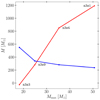 |
Fig. 6 Stellar mass formed in first megayear after formation of most massive star (blue) and the gas mass lost due to feedback Mloss,fb (red) versus the mass of the most massive star for simulations n3s3, n3s9, n3s4, and n3s1. Simulation names are labeled next to each red dot. This is the same interval as in Figure 5. |
3.4 Impact of resolution
In this subsection, we examine how the numerical resolution at the finest refinement level, n, affects the simulation results using the same random seed by comparison of models n3s1, n4s1, n5s1, and n6s1. Figure 9 shows the enclosed mass of stars and gas as a function of cluster radius for different refinement levels n. Higher-resolution simulations exhibit more efficient and centrally concentrated star formation, with stars forming closer to the cluster core compared to lower-resolution runs. This outcome is driven both by the ability of higher-resolution models to resolve higher gas densities, and by the adopted star formation scheme: stars are placed within the sink radius, which decreases as resolution increases. Consequently, higher-resolution simulations naturally favor more compact stellar distributions.
Since the rate of gas recombination is proportional to the square of the density, the ionizing luminosity from stars ionizes a smaller volume of gas at higher densities, thereby reducing the efficiency of the feedback. At the same time, the local free-fall time tff becomes shorter in denser regions, further accelerating central star formation. As a result, for n = 5 and 6 our simulations produce compact clusters with enclosed stellar masses, shown in Figure 9, which are consistent with the observations of Stutz (2018), as is discussed in Sect. 3.1.
Figure 10 shows the star formation rate (SFR) as a function of time. To emphasize differences in the star formation history, we smooth the result using a moving average with a window size of five snapshots, corresponding to ~50 kyr. For refinement level 3, star formation ceases by −1 Myr. In contrast, star formation continues until −1.75 Myr for refinement levels 4 and 5. At refinement level 6, a second star formation burst occurs at around 1.75 Myr, and star formation persists beyond 2 Myr.
Figure 4 shows gas density slices centered on the densest region in the simulations as a function of resolution. This figure shows that in simulations with refinement levels 3 and 4, stellar winds from the most massive stars, with masses M ≳ 24 M⊙, rapidly eject gas shortly after their formation, while efficient ionization by these clusters leads to the development of large ionized regions in their surroundings. In higher-resolution simulations, the threshold for sink formation is larger and the accretion radius is smaller (according to the Jeans criterion). This limits accretion to the densest regions, increasing local recombination rates and increasing the cooling rate in shocked stellar winds. As a result, stellar feedback becomes less efficient, slowing gas dispersal and producing smaller, denser, ionized regions. Refinement levels 5 and 6 can resolve filament- or sheet-like gas structures and localized star formation (see first columns in Fig. 4). These features are absent or poorly resolved in lower-resolution runs, underscoring the importance of both accretion radius and numerical resolution for achieving physical fidelity.
At level 6, the inefficiency of gas ejection and the long duration of star formation can be attributed to several factors. Simulations by Proszkow & Adams (2009) report that some young clusters (even younger than 5 Myr) remain gravitationally bound to the residual gas. Several factors may explain the reduced gas expulsion at high refinement levels: the presence of turbulent gas motions (Krumholz & McKee 2005), insufficient stellar feedback due to a lack of massive stars (Fall et al. 2010; Murray et al. 2010; Dale et al. 2014), or a deep gravitational potential from a highly concentrated gas distribution (Stutz 2018).
As we saw in Figure 10 above, refinement level 3 exhibits a sharp SFR peak and earlier gas dispersal than the other refinement levels, consistent with the results of the simulation by Li et al. (2019). They found that the central 80% of stars tend to form near the SFR peak (see their Fig. 2), typically in the range 0.6-1.4tff, with the peak occurring when about half of the stellar mass has formed. In our case, at refinement levels other than 3, the SFR peak occurs at about 1.1 Myr, but the stellar mass does not reach half of the final cluster mass. This may be due to the strong central concentration of our initial gas, which further collapses toward the center.
In the simulations of Chen et al. (2021), the centrally concentrated gas profile results in the SFR stopping at about 1.5 Myr (see their Fig. 3), and the peak time coincides with this same value. This may be because their MC has a large mass (8 × 10⁵ M⊙), the free-fall time is short, and stellar feedback is not effective due to recombination.
In summary, our results indicate that the total number and mass of stars formed seem to be approaching convergence. However, higher-resolution simulations yield more realistic ionized zones, stellar feedback, gas motion, and accretion flows.
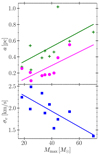 |
Fig. 7 Relationship between the maximum stellar mass (Mmax), the Plummer radius (apl) and the EFF scale radius (aeff) at 4tff, and the velocity dispersion (σv) for simulations at refinement level 3 with different random seeds. All quantities are measured using stars within the radius around the densest region of the cluster that encloses 95% of the total stellar mass. The green line shows a linear fit to apl (plus symbols), given by apl/(1pc) = (0.0091 ± 0.0041)[Mmax/(1 M⊙)] + 0.1608. The magenta line shows a linear fit to aeff (circle symbols), given by aeff/(1 pc) = (0.0084 ± 0.0035)[Mmax/(1 M⊙)] − 0.0437. The blue line shows a linear fit to σv (square symbols), given by σv/(1kms−1) = (−0.017 8 ± 0.0051)[Mmax/(1 M⊙)] + 2.6391. These linear fits are obtained with the linregress function from scipy.stats, which applies ordinary least-squares regression. The upper y-axis corresponds to apl and aeff in parsecs, while the lower y-axis represents σv in km s−1. |
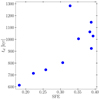 |
Fig. 8 Dependence of the duration of star formation, tsf, on the SFE for simulations performed at refinement level n = 3. Here, tsf is defined as the time interval from the onset of star formation until the gas mass enclosed within the radius containing half of the total stellar mass decreases to less than 20% of the stellar mass. |
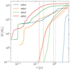 |
Fig. 9 Enclosed mass of the star cluster (solid lines) and of the gas (dashed lines) at 4.5 tff for different resolutions, with the maximum refinement level n given by the first digit of the model names. The half-mass radii of the star clusters at this time are indicated for each resolution by vertical dotted lines. |
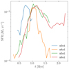 |
Fig. 10 Star formation rate as a function of time for different resolutions, with the maximum refinement level, n, given by the first digit of the model name. Higher-resolution results in more extended and sustained star formation activity. |
4 Model limitations
Several limitations of our modeling approach may influence the results and their interpretation. In this section, we discuss the constraints imposed by limited resolution and computational resources, the assumption of a partially virialized initial cloud, and the omission of a strong initial magnetic field.
Simulations with low refinement levels restrict the ability to resolve fine-scale gas structures, such as filaments or sheets, which are better captured at higher refinement levels. To mitigate this limitation, we also performed complementary simulations at higher-resolutions. At lower refinement levels, larger sink accretion radii (rsink = 0.64 pc for n = 3) allow star formation to occur in less dense regions, artificially enhancing feedback efficiency. By contrast, higher-resolution simulations with smaller sink radii (rsink = 0.08 pc for n = 6) resolve denser gas more accurately and produce more realistic ionized zones (see Section 3.4 for details).
The high computational cost of simulations at refinement levels n = 5 and n = 6 limited the number of realizations we could perform, particularly with different random seeds. At n = 3, we conducted ten realizations (n3s1-10) to capture statistical variations from stochastic IMF sampling, whereas for n = 46, only a single realization was feasible due to computational constraints (Table 1). For example, simulations at refinement levels n = 3, 4, 5, and 6 required approximately 7 days, 45 days, 4 months, and 7 months, respectively. At t = 4.5tff, the total number of grid cells reached 3 × 10⁵, 2 × 10⁶, 9 × 10⁶, and 3 × 10⁷ cells, respectively. Moreover, for n = 6, the simulations could not be run on fewer than 140 computing cores, and toward the end, the code advanced only ~10 kyr every three days.
Figure 11 presents gas density slices centered on the densest regions as a function of resolution. The figure shows that the overall gas dynamics are governed primarily by stellar feedback. Across different refinement levels, the evolution of gas and the onset of star formation proceed in a broadly similar manner, depending mainly on the mass of the most massive stars (compare the ionized regions in models n3s2 versus n4s1, n3s9 versus n5s1, and n3s3 versus n6s1). This suggests that the qualitative results obtained at refinement level n = 3 can be considered robust. Furthermore, subcluster formation occurs not only at n = 3 but also at higher-resolutions, such as n = 4 (model n4s1). In model n3s3, the snapshot indicated by a ★ is shown 40 kyr earlier than 4tff, since a very massive star of 60 M⊙ forms shortly afterward. At the displayed epoch, however, the primary feedback effect arises from an 18 M⊙ star, which governs the gas evolution at that stage.
The deviation of our stellar cluster profiles from analytical models may partly result from only balancing kinetic and gravitational energy globally but not locally (see Sect. 2.6) and from the neglect of strong initial magnetic fields (Hennebelle et al. 2011; Federrath & Klessen 2012; Fontani et al. 2016; Wu et al. 2020). The initial cloud is set up with a virial parameter αvir = 0.5, indicating that the total turbulent kinetic energy is half the gravitational potential energy (Section 2.6). This does not fully capture the energy balance of the initialized clouds, though, since centrally concentrated clouds require stronger central turbulent support to balance their deep gravitational potentials.
A fully virialized cloud could delay global collapse, extend the duration of star formation (tsf), and increase SFE by providing greater support against rapid central collapse. This would likely produce more spatially distributed star formation and less compact stellar clusters. However, unless there were a physical mechanism to drive the turbulence in a centrally concentrated matter, the turbulence would decay in a free-fall time (Mac Low 1999) and the cloud would then evolve without much change.
Indeed, numerical studies have shown that clouds with higher virial parameters undergo more fragmented star formation, leading to the formation of multiple subclusters rather than a single, centrally concentrated cluster (Bonnell et al. 2003; Clark et al. 2005; Federrath & Klessen 2012). In our case, increasing αvir could promote subcluster formation (as is shown in n3s6, n3s7, and n4s1 by Figure 3), yielding stellar density profiles that deviate from the analytical Plummer model ( a* = 1.1 pc) and resemble EFF profiles with variable γeff (Section 3.1). Such conditions would likely increase the fitted scale radii (apl, aeff), producing less compact clusters.
Our simulations neglect the role of strong magnetic fields, which is a significant simplification. Magnetic fields provide additional support against gravitational collapse, influence gas dynamics, and modulate the efficiency of stellar feedback. Previous studies have shown that magnetic fields can reduce the fragmentation of MCs, delay star formation, and alter the morphology of ionized regions (McKee & Ostriker 2007; Padoan & Nordlund 2011; Federrath 2015). Including stronger magnetic fields in our models could therefore lead to reduced star formation rates, larger characteristic scales of stellar clustering, and modified feedback-driven gas expulsion.
In summary, our results are shaped by several key modeling assumptions and constraints. Limited resolution and high computational cost restrict the number of realizations at the highest refinement levels, though comparisons across resolutions suggest that low-resolution runs capture the essential physics of feedback-driven gas dispersal. The assumption of a partially virialized initial cloud likely biases our clusters toward higher central concentrations than might occur in fully virialized systems, where turbulence would delay collapse and promote greater subclustering. Finally, the omission of strong magnetic fields removes an important source of support and regulation of fragmentation, potentially leading to higher star formation rates and more compact stellar structures than would otherwise be expected.
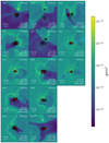 |
Fig. 11 Snapshots of gas density and stellar distribution at 4tff for different maximum grid resolutions. The ionization fronts are marked with cyan lines. Stars are shown as black dots; massive stars are highlighted in red, with sizes proportional to their masses. In each panel, the following notations are used: (bottom left) physical scale; (bottom right) the mass of the most massive star, total stellar mass, and number of stars; (top left) model label; (top right) simulation time. The color scale indicates the gas density in grams per cubic centimetre. The panel for model n3s3, marked with a ★ (simulation time), is shown 40 kyr earlier than 4tff, because a 60 M⊙ star forms shortly afterward; at the displayed time, the feedback is dominated by an 18 M⊙ star. |
5 Conclusion
In this study, we have investigated how massive star formation and gas structure influence the formation and evolution of young star clusters. Using simulations with varying numerical resolution and massive star formation occurrence, we followed the collapse, star formation, and feedback processes to determine their role in regulating cluster properties.
The evolution of our simulations can be summarized as follows: gravitational collapse begins globally toward the center of the cloud, possibly leading to the formation of sub-structures resembling filaments or sheets and the first stars appear at approximately 1tff ; accretion then continues in the central region, fuelling further star formation; this process becomes progressively less efficient as the most massive stars form, marking the onset of stellar feedback. We find the following conclusions.
The gas in the central regions has shorter free-fall times, leading to rapid collapse and intense star formation, while gas in the outer regions has longer free-fall times (see Fig. 1), so it cannot form stars prior to falling in to the center;
As a result, star formation produces rather more centrally concentrated profiles (Fig. 2) predicted from the initial gas distribution by the local collapse theory of Parmentier & Pfalzner (2013);
Stars often form in subclusters along filament- or sheet-like gas structures, even in the highly centralized initial gas distributions studied here. Early-forming massive stars promote the formation of interacting subclusters (see Fig. 3). In some models, the subcluster merge into a single cluster, while in others they survive separately. The evolution of such subclusters in less centrally concentrated gas was described by Cournoyer-Cloutier et al. (2023);
The masses of the most massive stars are critical in determining the strength of stellar feedback and shaping the evolution of young star clusters (Figs. 5-7). This extends the results from Lewis et al. (2023) to more centrally concentrated initial conditions and a range of massive star formation times;
The final SFE is influenced by both the mass of the most massive star formed and the duration of star formation, tsf (see Figs. 5 and 8);
Our convergence study shows that the total number and mass of stars formed appear to be approaching convergence at our highest grid resolutions (Figs. 9 and 10). However, higher grid resolution continues to improve the modeling of ionized zones, stellar feedback, and accretion in dense regions (Fig. 11).
However, these conclusions should be interpreted in light of the limitations of our models, which include assumptions about numerical resolution, cloud virialization, and the absence of strong initial magnetic fields. A detailed discussion of these caveats is provided in Section 4. Addressing these limitations in future work will be crucial for building a more comprehensive picture of star cluster formation in realistic MC environments.
Data availability
All density visualization videos and corresponding snapshot files generated from the simulations and used in this study are publicly available at Zenodo.
Acknowledgements
We thank the anonymous referee for the constructive comments and suggestions that helped improve the clarity and quality of this paper. The authors thank S. Portegies Zwart, S. L. McMillan, E. P. Andersson, and S. M. Appel for scientific discussions and extensive support in our use of the AMUSE and Torch software. This research has been funded by the Science Committee of the Ministry of Science and Higher Education, Republic of Kazakhstan (Grant No. AP19677351). AA acknowledges support from a Bolashaq International Scholarship. M-MML and BP acknowledge support from the US NSF grant AST23-07950. CC-C acknowledges funding from a Canada Graduate Scholarship-Doctoral (CGS D) from NSERC. EA’s work is supported by Nazarbayev University Faculty Development Competitive Research Grant Program (no. 040225FD4713). Some computations presented here were performed on Snellius through the Dutch National Supercomputing Center SURF grants 15220 and 2023/ENW/01498863. M-MML thanks the Institut für Theoretische Astrophysik of Heidelberg University for hospitality during work on this paper.
References
- Adams, F. C. 2000, ApJ, 542, 964 [NASA ADS] [CrossRef] [Google Scholar]
- Agertz, O., Kravtsov, A. V., Leitner, S. N., & Gnedin, N. Y. 2013, ApJ, 770, 25 [NASA ADS] [CrossRef] [Google Scholar]
- Alina, D., Ristorcelli, I., Montier, L., et al. 2019, MNRAS, 485, 2825 [Google Scholar]
- Baczynski, C., Glover, S. C. O., & Klessen, R. S. 2015, MNRAS, 454, 380 [CrossRef] [Google Scholar]
- Bate, M. R., Bonnell, I. A., & Price, N. M. 1995, MNRAS, 277, 362 [Google Scholar]
- Baumgardt, H., & Kroupa, P. 2007, MNRAS, 380, 1589 [NASA ADS] [CrossRef] [Google Scholar]
- Bissekenov, A., Kalambay, M., Abdikamalov, E., et al. 2024a, A&A, 689, A282 [NASA ADS] [CrossRef] [EDP Sciences] [Google Scholar]
- Bissekenov, A., Kalambay, M. T., Abylkairov, Y. S., & Shukirgaliyev, B. T. 2024b, Recent Contrib. Phys., 90, 3 [Google Scholar]
- Bissekenov, A., Pang, X., Kamlah, A., et al. 2025, A&A, 699, A196 [NASA ADS] [CrossRef] [EDP Sciences] [Google Scholar]
- Bonnell, I. A., Bate, M. R., & Vine, S. G. 2003, MNRAS, 343, 413 [NASA ADS] [CrossRef] [Google Scholar]
- Brinkmann, N., Banerjee, S., Motwani, B., & Kroupa, P. 2017, A&A, 600, A49 [NASA ADS] [CrossRef] [EDP Sciences] [Google Scholar]
- Burki, G. 1978, A&A, 62, 159 [Google Scholar]
- Canning, R. E. A., Ryon, J. E., Gallagher, J. S., et al. 2014, MNRAS, 444, 336 [CrossRef] [Google Scholar]
- Chen, H.-C., & Ko, C.-M. 2009, ApJ, 698, 1659 [Google Scholar]
- Chen, Y., Li, H., & Vogelsberger, M. 2021, MNRAS, 502, 6157 [Google Scholar]
- Clark, P. C., Bonnell, I. A., Zinnecker, H., & Bate, M. R. 2005, MNRAS, 359, 809 [NASA ADS] [CrossRef] [Google Scholar]
- Colella, P., & Woodward, P. R. 1984, J. Computai. Phys., 54, 174 [Google Scholar]
- Cournoyer-Cloutier, C., Tran, A., Lewis, S., et al. 2021, MNRAS, 501, 4464 [NASA ADS] [CrossRef] [Google Scholar]
- Cournoyer-Cloutier, C., Sills, A., Harris, W. E., et al. 2023, MNRAS, 521, 1338 [NASA ADS] [CrossRef] [Google Scholar]
- Cournoyer-Cloutier, C., Sills, A., Harris, W. E., et al. 2024, arXiv e-prints [arXiv:2410.07433] [Google Scholar]
- Dale, J. E., Ngoumou, J., Ercolano, B., & Bonnell, I. A. 2014, MNRAS, 442, 694 [Google Scholar]
- Dale, D. A., Graham, G. B., Barnes, A. T., et al. 2025, AJ, 169, 133 [Google Scholar]
- Draine, B. T. 2011, Physics of the Interstellar and Intergalactic Medium (Princeton: Princeton University Press) [Google Scholar]
- Dubey, A., Antypas, K., Calder, A. C., et al. 2014, Int. J. High Performance Comput. Appl., 28, 225 [Google Scholar]
- Elmegreen, B. G., & Scalo, J. 2004, ARA&A, 42, 211 [Google Scholar]
- Elson, R. A. W., Fall, S. M., & Freeman, K. C. 1987, ApJ, 323, 54 [Google Scholar]
- Fall, S. M., Krumholz, M. R., & Matzner, C. D. 2010, ApJ, 710, L142 [NASA ADS] [CrossRef] [Google Scholar]
- Farias, J. P., & Tan, J. C. 2023, MNRAS, 523, 2083 [NASA ADS] [CrossRef] [Google Scholar]
- Farias, J. P., Tan, J. C., & Chatterjee, S. 2019, MNRAS, 483, 4999 [NASA ADS] [CrossRef] [Google Scholar]
- Federrath, C. 2015, MNRAS, 450, 4035 [Google Scholar]
- Federrath, C., & Klessen, R. S. 2012, ApJ, 761, 156 [Google Scholar]
- Federrath, C., Banerjee, R., Clark, P. C., & Klessen, R. S. 2010, ApJ, 713, 269 [NASA ADS] [CrossRef] [Google Scholar]
- Feigelson, E. D., Getman, K., Townsley, L., et al. 2005, ApJS, 160, 379 [Google Scholar]
- Fierlinger, K. M., Burkert, A., Ntormousi, E., et al. 2016, MNRAS, 456, 710 [NASA ADS] [CrossRef] [Google Scholar]
- Fontani, F., Commerçon, B., Giannetti, A., et al. 2016, A&A, 593, L14 [NASA ADS] [CrossRef] [EDP Sciences] [Google Scholar]
- Fryxell, B., Olson, K., Ricker, P., et al. 2000, ApJS, 131, 273 [Google Scholar]
- Fujii, M., Iwasawa, M., Funato, Y., & Makino, J. 2007, PASJ, 59, 1095 [NASA ADS] [Google Scholar]
- Goodwin, S. P. 1997, MNRAS, 284, 785 [Google Scholar]
- Goodwin, S. P. 2009, Ap&SS, 324, 259 [Google Scholar]
- Goodwin, S. P., & Bastian, N. 2006, MNRAS, 373, 752 [Google Scholar]
- Grudic, M. Y., Hopkins, P. F., Faucher-Giguère, C.-A., et al. 2018, MNRAS, 475, 3511 [CrossRef] [Google Scholar]
- Gusev, A. S., Sakhibov, F. K., Piskunov, A. E., et al. 2016, Astron. Astrophys. Trans., 29, 293 [Google Scholar]
- Härer, L., Vieu, T., & Reville, B. 2025, A&A, 698, A6 [NASA ADS] [CrossRef] [EDP Sciences] [Google Scholar]
- Haworth, T. J., Glover, S. C. O., Koepferl, C. M., Bisbas, T. G., & Dale, J. E. 2018, New A Rev., 82, 1 [NASA ADS] [CrossRef] [Google Scholar]
- Heitsch, F., Mac Low, M.-M., & Klessen, R. S. 2001, ApJ, 547, 280 [NASA ADS] [CrossRef] [Google Scholar]
- Hennebelle, P., Commerçon, B., Joos, M., et al. 2011, A&A, 528, A72 [NASA ADS] [CrossRef] [Google Scholar]
- Heydari-Malayeri, M., Charmandaris, V., Deharveng, L., et al. 2003, in IAU Symposium, 212, A Massive Star Odyssey: From Main Sequence to Supernova, eds. K. van der Hucht, A. Herrero, & C. Esteban (San Francisco: Astron. Soc. Pacific), 553 [Google Scholar]
- Hopkins, P. F., Quataert, E., & Murray, N. 2012, MNRAS, 421, 3522 [Google Scholar]
- Hut, P., Makino, J., & McMillan, S. 1995, ApJ, 443, L93 [NASA ADS] [CrossRef] [Google Scholar]
- Ibáñez-Mejía, J. C., Mac Low, M.-M., Klessen, R. S., & Baczynski, C. 2016, ApJ, 824, 41 [Google Scholar]
- Ibáñez-Mejía, J. C., Mac Low, M.-M., Klessen, R. S., & Baczynski, C. 2017, ApJ, 850, 62 [Google Scholar]
- Ishchenko, M., Masliukh, V., Hradov, M., et al. 2025, A&A, 694, A33 [NASA ADS] [CrossRef] [EDP Sciences] [Google Scholar]
- Jeans, J. H. 1902, Roy. Soc. Lond. Phil. Trans. Ser. A, 199, 1 [Google Scholar]
- Kalambay, M. T., Naurzbayeva, A. Z., Otebay, A. B., et al. 2022, Recent Contrib. Phys., 83, 4 [Google Scholar]
- Kalambay, M. T., Otebay, A. B., Nazar, A. B., Assilkhan, A., & Shukirgaliyev, B. T. 2025, Herald Kazakh-British Tech. Univ., 22, 312 [Google Scholar]
- Karam, J., & Sills, A. 2022, MNRAS, 513, 6095 [Google Scholar]
- Karam, J., & Sills, A. 2024, ApJ, 967, 86 [Google Scholar]
- Kim, J.-G., Kim, W.-T., & Ostriker, E. C. 2018, ApJ, 859, 68 [NASA ADS] [CrossRef] [Google Scholar]
- Kolmogorov, A. 1941, Akad. Nauk SSSR Dokl., 30, 301 [Google Scholar]
- Komesh, T., Garay, G., Henkel, C., et al. 2024, ApJ, 967, 15 [Google Scholar]
- Kroupa, P. 2002, Science, 295, 82 [Google Scholar]
- Krumholz, M. R., & McKee, C. F. 2005, ApJ, 630, 250 [Google Scholar]
- Krumholz, M. R., McKee, C. F., & Klein, R. I. 2004, ApJ, 611, 399 [NASA ADS] [CrossRef] [Google Scholar]
- Kuhn, M. A., Feigelson, E. D., Getman, K. V., et al. 2015, ApJ, 812, 131 [NASA ADS] [CrossRef] [Google Scholar]
- Lada, C. J., & Lada, E. A. 2003, ARA&A, 41, 57 [Google Scholar]
- Lada, C. J., Margulis, M., & Dearborn, D. 1984, ApJ, 285, 141 [NASA ADS] [CrossRef] [Google Scholar]
- Lanz, T., & Hubeny, I. 2003, ApJS, 146, 417 [NASA ADS] [CrossRef] [Google Scholar]
- Larson, R. B. 1981, MNRAS, 194, 809 [Google Scholar]
- Laverde-Villarreal, E., Sills, A., Cournoyer-Cloutier, C., & Arias Callejas, V. 2025, ApJ, accepted [arXiv:2507.00815] [Google Scholar]
- Leisawitz, D., Bash, F. N., & Thaddeus, P. 1989, ApJS, 70, 731 [NASA ADS] [CrossRef] [Google Scholar]
- Levenberg, K. 1944, Q. Appl. Math., 2, 164 [Google Scholar]
- Lewis, S. C., McMillan, S. L. W., Mac Low, M.-M., et al. 2023, ApJ, 944, 211 [NASA ADS] [CrossRef] [Google Scholar]
- Li, H., Vogelsberger, M., Marinacci, F., & Gnedin, O. Y. 2019, MNRAS, 487, 364 [NASA ADS] [CrossRef] [Google Scholar]
- Löhner, R. 1987, Comput. Methods Appl. Mech. Eng., 61, 323 [CrossRef] [Google Scholar]
- Mac Low, M.-M. 1999, ApJ, 524, 169 [Google Scholar]
- McKee, C. F., & Ostriker, E. C. 2007, ARA&A, 45, 565 [Google Scholar]
- McMillan, S., Portegies Zwart, S., van Elteren, A., & Whitehead, A. 2012, in Astronomical Society of the Pacific Conference Series, 453, Advances in Computational Astrophysics: Methods, Tools, and Outcome, eds. R. Capuzzo-Dolcetta, M. Limongi, & A. Tornambè, 129 [Google Scholar]
- Megeath, S. T., Gutermuth, R., Muzerolle, J., et al. 2016, AJ, 151, 5 [Google Scholar]
- Miyoshi, T., & Kusano, K. 2005, J. Computat. Phys., 208, 315 [NASA ADS] [CrossRef] [Google Scholar]
- Motte, F., Bontemps, S., Csengeri, T., et al. 2022, A&A, 662, A8 [NASA ADS] [CrossRef] [EDP Sciences] [Google Scholar]
- Murray, N., Quataert, E., & Thompson, T. A. 2010, ApJ, 709, 191 [NASA ADS] [CrossRef] [Google Scholar]
- Myers, P. C. 2009, ApJ, 700, 1609 [Google Scholar]
- O’Connell, R. W. 2004, in Astronomical Society of the Pacific Conference Series, 322, The Formation and Evolution of Massive Young Star Clusters, eds. H. J. G. L. M. Lamers, L. J. Smith, & A. Nota (San Francisco: Astron. Soc. Pacific), 551 [Google Scholar]
- O’Dell, C. R. 2001, ARA&A, 39, 99 [Google Scholar]
- Padoan, P., & Nordlund, Â. 2011, ApJ, 730, 40 [NASA ADS] [CrossRef] [Google Scholar]
- Parmentier, G., & Pfalzner, S. 2013, A&A, 549, A132 [NASA ADS] [CrossRef] [EDP Sciences] [Google Scholar]
- Pelupessy, F. I., & Portegies Zwart, S. 2012, MNRAS, 420, 1503 [NASA ADS] [CrossRef] [Google Scholar]
- Pelupessy, F. I., van Elteren, A., de Vries, N., et al. 2013, A&A, 557, A84 [NASA ADS] [CrossRef] [EDP Sciences] [Google Scholar]
- Plummer, H. C. 1911, MNRAS, 71, 460 [Google Scholar]
- Polak, B., Mac Low, M.-M., Klessen, R. S., et al. 2024, A&A, 690, A94 [NASA ADS] [CrossRef] [EDP Sciences] [Google Scholar]
- Polak, B., Mac Low, M.-M., Klessen, R. S., et al. 2025, A&A, 695, A188 [NASA ADS] [CrossRef] [EDP Sciences] [Google Scholar]
- Portegies Zwart, S., & McMillan, S. 2018, Astrophysical Recipes; The art of AMUSE (IOP Publishing) [Google Scholar]
- Portegies Zwart, S. F., & Verbunt, F. 1996, A&A, 309, 179 [NASA ADS] [Google Scholar]
- Portegies Zwart, S., McMillan, S., Harfst, S., et al. 2009, New A, 14, 369 [NASA ADS] [CrossRef] [Google Scholar]
- Portegies Zwart, S., McMillan, S. L. W., van Elteren, E., Pelupessy, I., & de Vries, N. 2013, Comput. Phys. Commun., 184, 456 [Google Scholar]
- Portegies Zwart, S., van Elteren, A., Pelupessy, I., et al. 2019, AMUSE: the Astrophysical Multipurpose Software Environment [Google Scholar]
- Portegies Zwart, S., Pelupessy, I., Martínez-Barbosa, C., van Elteren, A., & McMillan, S. 2020, Commun. Nonlinear Sci. Numer. Simul., 85, 105240 [Google Scholar]
- Proszkow, E.-M., & Adams, F. C. 2009, ApJS, 185, 486 [NASA ADS] [CrossRef] [Google Scholar]
- Rahner, D., Pellegrini, E. W., Glover, S. C. O., & Klessen, R. S. 2019, MNRAS, 483, 2547 [NASA ADS] [CrossRef] [Google Scholar]
- Rhea, C. L., Hlavacek-Larrondo, J., Gendron-Marsolais, M.-L., et al. 2025, AJ, 169, 203 [Google Scholar]
- Ricker, P. M. 2008, ApJS, 176, 293 [NASA ADS] [CrossRef] [Google Scholar]
- Rogers, H., & Pittard, J. M. 2013, MNRAS, 431, 1337 [CrossRef] [Google Scholar]
- Sales, L. V., Marinacci, F., Springel, V., & Petkova, M. 2014, MNRAS, 439, 2990 [Google Scholar]
- Schroetter, I., Berne, O., Boyden, R., et al. 2025, A MIRI spectroscopic atlas of irradiated disks in Orion, JWST Proposal. Cycle 4, ID. #7534 [Google Scholar]
- Seifried, D., Walch, S., Reissl, S., & Ibáñez-Mejía, J. C. 2019, MNRAS, 482, 2697 [NASA ADS] [CrossRef] [Google Scholar]
- Shukirgaliyev, B. 2018, PhD thesis, Astronomisches Rechen-Institut [Google Scholar]
- Shukirgaliyev, B., Parmentier, G., Berczik, P., & Just, A. 2017, A&A, 605, A119 [NASA ADS] [CrossRef] [EDP Sciences] [Google Scholar]
- Shukirgaliyev, B., Parmentier, G., Just, A., & Berczik, P. 2018, ApJ, 863, 171 [Google Scholar]
- Shukirgaliyev, B., Otebay, A., Just, A., et al. 2019a, Proc. Natl Acad. Sci. Rep. Kazakhstan Phys. Math. Ser., 3, 130 [Google Scholar]
- Shukirgaliyev, B., Parmentier, G., Berczik, P., & Just, A. 2019b, MNRAS, 486, 1045 [NASA ADS] [CrossRef] [Google Scholar]
- Shukirgaliyev, B., Parmentier, G., Berczik, P., & Just, A. 2020, in IAU Symposium, 351, Star Clusters: From the Milky Way to the Early Universe, eds. A. Bragaglia, M. Davies, A. Sills, & E. Vesperini (Cambridge, UK: Cambridge U. Press), 507 [Google Scholar]
- Shukirgaliyev, B., Otebay, A., Sobolenko, M., et al. 2021, A&A, 654, A53 [NASA ADS] [CrossRef] [EDP Sciences] [Google Scholar]
- Simpson, C. M., Bryan, G. L., Hummels, C., & Ostriker, J. P. 2015, ApJ, 809, 69 [NASA ADS] [CrossRef] [Google Scholar]
- Smith, R., Fellhauer, M., Goodwin, S., & Assmann, P. 2011, MNRAS, 414, 3036 [CrossRef] [Google Scholar]
- Sormani, M. C., Treß, R. G., Klessen, R. S., & Glover, S. C. O. 2017, MNRAS, 466, 407 [NASA ADS] [CrossRef] [Google Scholar]
- Springel, V. 2010, MNRAS, 401, 791 [Google Scholar]
- Stahler, S. W., & Palla, F. 2004, The Formation of Stars (Wiley), 865 [Google Scholar]
- Stutz, A. M. 2018, MNRAS, 473, 4890 [NASA ADS] [CrossRef] [Google Scholar]
- Toonen, S., Nelemans, G., & Portegies Zwart, S. 2012, A&A, 546, A70 [NASA ADS] [CrossRef] [EDP Sciences] [Google Scholar]
- Truelove, J. K., Klein, R. I., McKee, C. F., et al. 1997, ApJ, 489, L179 [CrossRef] [Google Scholar]
- Ussipov, N., Akhmetali, A., Zaidyn, M., et al. 2024, Eurasian Phys. Tech. J., 21, 108 [CrossRef] [Google Scholar]
- Virtanen, P., Gommers, R., Oliphant, T. E., et al. 2020, Nat. Methods, 17, 261 [Google Scholar]
- Wall, J. E., McMillan, S. L. W., Mac Low, M.-M., Klessen, R. S., & Portegies Zwart, S. 2019, ApJ, 887, 62 [NASA ADS] [CrossRef] [Google Scholar]
- Wall, J. E., Mac Low, M.-M., McMillan, S. L. W., et al. 2020, ApJ, 904, 192 [Google Scholar]
- Weis, L., West, C., Just, A., et al. 2025, A&A, 703, A47 [NASA ADS] [CrossRef] [EDP Sciences] [Google Scholar]
- Wise, J. H., & Abel, T. 2011, MNRAS, 414, 3458 [NASA ADS] [CrossRef] [Google Scholar]
- Wu, B., Tan, J. C., Christie, D., & Nakamura, F. 2020, ApJ, 891, 168 [Google Scholar]
- Wünsch, R. 2015, Highlights Astron., 16, 614 [Google Scholar]
- Yan, Z., Jerabkova, T., & Kroupa, P. 2023, A&A, 670, A151 [NASA ADS] [CrossRef] [EDP Sciences] [Google Scholar]
- Zhang, W., Zhou, J., Esimbek, J., et al. 2024a, A&A, 688, A99 [NASA ADS] [CrossRef] [EDP Sciences] [Google Scholar]
- Zhang, W., Zhou, J., Esimbek, J., et al. 2024b, ApJS, 275, 7 [Google Scholar]
Appendix A Density profile of unprocessed gas
Parmentier & Pfalzner (2013) proposed a semi-analytical model in which a star cluster is formed from a centrally concentrated spherically symmetric gas cloud with constant SFE per free-fall time εff. The overall density profile ρ0(r) does not change, where r is the distance from the center of the cluster. As stars form, the gas profile ρgas(r, t) and the star profile ρ*(r, t) change depending on the evolution time t, but must satisfy the constraint
 (A.1)
(A.1)
Parmentier & Pfalzner (2013) derive the gas and stellar profile evolution to be
 (A.2)
(A.2)
 (A.3)
(A.3)
where G is the gravitational constant. Shukirgaliyev et al. (2017) rewrote the constraint for a given density profile of the formed star cluster ρ*(r),
 (A.4)
(A.4)
In this formulation, the gas profile ρgas and the total density profile ρ0 depend on the star formation duration tSF and are calculated using Eqs. (A.2) and (A.3), which results in
 (A.5)
(A.5)
where

and

All Tables
All Figures
|
Fig. 1 Initial density and free-fall time, teff, of the cluster derived by Shukirgaliyev et al. (2017) as a function of radius. The initial gas density (Eq. (5)) is shown in green, the final stellar density (Eq. (4)) in red, and the final gas density (Eq. (6)) in orange. The initial density profile is used directly in the simulation setup. The free-fall time, tff, of the initial gas density distribution as a function of radius is shown in (solid blue). The horizontal dashed blue line indicates the free-fall time corresponding to the average density, while the vertical dotted blue line marks the half-mass radius, rh, of the initial gas distribution. The local value of tff is shortest in the central regions and increases significantly toward larger radii. |
| In the text | |
|
Fig. 2 Stellar density profiles at 4tff (blue points) are compared with the analytically predicted Plummer profile for the stellar distribution (dashed orange line), as well as best-fit Plummer (dashed green) and EFF (dash-dotted magenta) models. The mass of the most massive star formed in each simulation is indicated in the lower left corner of each panel. The panel marked with a ★ (n3s3) is shown at a slightly earlier time; see also the text for details on subcluster cases. |
| In the text | |
|
Fig. 3 Gas density slices and stellar distribution projections from the n3s6, n3s7, and n4s1 models. In these models subcluster formation occurs. For n3s6 and n3s7: (top row) onset of stellar feedback; (middle row) prior to the formation of the second cluster; (bottom row) after the formation of the second cluster. For n4s1: (top row) two clusters are present; (middle row) clusters merge into a single structure; (bottom row) the system separates again into two clusters. Ionization fronts are indicated by the cyan line. Black dots indicate individual stars, with massive stars shown in red. The symbol size of massive stars is proportional to their mass. Annotations in each panel include: (bottom left) scale bar; (bottom right) mass of the most massive star, total stellar mass within 5.5 pc, and total number of stars; (top left) simulation label; (top right) simulation time. The color scale represents the gas density in grams per cubic centimetre. |
| In the text | |
|
Fig. 4 Images of gas density and stellar distribution at different times for different maximum grid resolutions (higher refinement level n corresponds to finer grid resolution). Each row corresponds to a level; each column, to a simulation time (1.5 tff, 3 tff, 4.5 tff). The ionization fronts are marked with cyan lines. Stars are black dots; massive stars are red, with sizes proportional to their masses. In each panel, the notations are as follows: (bottom left) physical scale; (bottom right) the mass of the most massive star, total stellar mass, and number of stars; (top left) model label; (top right) simulation time. The color scale represents the gas density in grams per cubic centimetre. |
| In the text | |
|
Fig. 5 Slices of gas density and projected stellar distribution at the formation time in each model of the most massive star with M > 15 M⊙ (left column), and 1 Myr later (right column), for the n3s3, n3s9, n3s4, and n3s1 simulations. Ionization fronts are indicated by cyan lines. Black dots represent stars, while massive stars are shown in red; massive star symbol sizes are proportional to stellar mass. In n3s1, two most massive stars form: one with 50 M⊙ at 891 kyr (triggering feedback), and a second with 53 M⊙ at 1187 kyr. Annotations in each panel are (bottom left) physical scale; (bottom right) mass of the most massive star, total stellar mass within 5.5 pc, total gas mass within 5.5 pc, and number of stars; (top left) model; (top right) simulation time. The color scale represents the gas density. |
| In the text | |
|
Fig. 6 Stellar mass formed in first megayear after formation of most massive star (blue) and the gas mass lost due to feedback Mloss,fb (red) versus the mass of the most massive star for simulations n3s3, n3s9, n3s4, and n3s1. Simulation names are labeled next to each red dot. This is the same interval as in Figure 5. |
| In the text | |
|
Fig. 7 Relationship between the maximum stellar mass (Mmax), the Plummer radius (apl) and the EFF scale radius (aeff) at 4tff, and the velocity dispersion (σv) for simulations at refinement level 3 with different random seeds. All quantities are measured using stars within the radius around the densest region of the cluster that encloses 95% of the total stellar mass. The green line shows a linear fit to apl (plus symbols), given by apl/(1pc) = (0.0091 ± 0.0041)[Mmax/(1 M⊙)] + 0.1608. The magenta line shows a linear fit to aeff (circle symbols), given by aeff/(1 pc) = (0.0084 ± 0.0035)[Mmax/(1 M⊙)] − 0.0437. The blue line shows a linear fit to σv (square symbols), given by σv/(1kms−1) = (−0.017 8 ± 0.0051)[Mmax/(1 M⊙)] + 2.6391. These linear fits are obtained with the linregress function from scipy.stats, which applies ordinary least-squares regression. The upper y-axis corresponds to apl and aeff in parsecs, while the lower y-axis represents σv in km s−1. |
| In the text | |
|
Fig. 8 Dependence of the duration of star formation, tsf, on the SFE for simulations performed at refinement level n = 3. Here, tsf is defined as the time interval from the onset of star formation until the gas mass enclosed within the radius containing half of the total stellar mass decreases to less than 20% of the stellar mass. |
| In the text | |
|
Fig. 9 Enclosed mass of the star cluster (solid lines) and of the gas (dashed lines) at 4.5 tff for different resolutions, with the maximum refinement level n given by the first digit of the model names. The half-mass radii of the star clusters at this time are indicated for each resolution by vertical dotted lines. |
| In the text | |
|
Fig. 10 Star formation rate as a function of time for different resolutions, with the maximum refinement level, n, given by the first digit of the model name. Higher-resolution results in more extended and sustained star formation activity. |
| In the text | |
|
Fig. 11 Snapshots of gas density and stellar distribution at 4tff for different maximum grid resolutions. The ionization fronts are marked with cyan lines. Stars are shown as black dots; massive stars are highlighted in red, with sizes proportional to their masses. In each panel, the following notations are used: (bottom left) physical scale; (bottom right) the mass of the most massive star, total stellar mass, and number of stars; (top left) model label; (top right) simulation time. The color scale indicates the gas density in grams per cubic centimetre. The panel for model n3s3, marked with a ★ (simulation time), is shown 40 kyr earlier than 4tff, because a 60 M⊙ star forms shortly afterward; at the displayed time, the feedback is dominated by an 18 M⊙ star. |
| In the text | |
Current usage metrics show cumulative count of Article Views (full-text article views including HTML views, PDF and ePub downloads, according to the available data) and Abstracts Views on Vision4Press platform.
Data correspond to usage on the plateform after 2015. The current usage metrics is available 48-96 hours after online publication and is updated daily on week days.
Initial download of the metrics may take a while.