| Issue |
A&A
Volume 706, February 2026
|
|
|---|---|---|
| Article Number | A166 | |
| Number of page(s) | 25 | |
| Section | Planets, planetary systems, and small bodies | |
| DOI | https://doi.org/10.1051/0004-6361/202449545 | |
| Published online | 16 February 2026 | |
A super-Earth orbiting the early-M dwarf GJ7★
1
Centro de Astrobiología, CSIC-INTA,
Camino Bajo del Castillo s/n,
28692
Villanueva de la Cañada, Madrid,
Spain
2
Instituto de Astrolísica de Canarias,
Avda. Vía Láctea s/n,
38205
La Laguna, Tenerile,
Spain
3
Dept. Astrolísica, Universidad de La Laguna,
38206
La Laguna, Tenerile,
Spain
4
Instituto de Astrolísica e Ciências do Espaço, Universidade do Porto, CAUP,
Rua das Estrelas,
4150-762
Porto,
Portugal
5
Dept. de Física e Astronomia, Faculdade de Ciências, Universidade do Porto,
Rua Campo Alegre,
4169-007
Porto,
Portugal
6
Observatoire de l’Université de Genève,
51 chemin Pegasi,
1290
Sauverny,
Switzerland
7
Light Bridges S.L.,
Avda. Alcalde Ramírez Bethencourt, 17,
35004
Las Palmas de Gran Canaria,
Spain
8
INAF–Osservatorio Astrofisico di Torino,
Via Osservatorio 20,
10025
Pino Torinese,
Italy
9
INAF–Osservatorio Astronomico di Trieste,
Via G.B. Tiepolo, 11,
34143
Trieste,
Italy
10
IFPU – Institute lor Fundamental Physics ol the Universe,
via Beirut 2,
34151
Trieste,
Italy
11
INFN–National Institute lor Nuclear Physics,
via Valerio 2,
34127
Trieste,
Italy
12
Space Research and Planetary Sciences, Physics Institute, University ol Bern,
Bern,
Switzerland
13
Center lor Space and Habitability, University ol Bern,
Bern,
Switzerland
14
Dept. de Matemática y Física Aplicadas, Univ. Católica de la Santísima Concepción,
Alonso de Rivera
2850,
Concepción,
Chile
15
Centro de Astrolísica do Universidade do Porto,
Rua das Estrelas,
4150-762
Porto,
Portugal
16
Observatoire François-Xavier Bagnoud – OFXB,
3961
Saint-Luc,
Switzerland
★★ Corresponding author: This email address is being protected from spambots. You need JavaScript enabled to view it.
Received:
8
February
2024
Accepted:
17
November
2025
Abstract
We aim to characterize the nearby (23.78 pc), low-mass planetary system GJ7 (TOI-198), which consists of an M0-type star and a terrestrial planet. Using photometric data from three sectors of the Transiting Exoplanet Survey Satellite (TESS) and a follow-up on the planetary transit observed by the Characterizing ExOPlanets Satellite (CHEOPS), along with 87 precise radial velocities obtained with the Echelle SPectrograph lor Rocky Exoplanets and Stable Spectroscopic Observations (ESPRESSO) spectrograph, we confidently confirm the planet and infer its properties. Planet GJ7 b has a mass of Mp = 3.17−0.65+0.64 M⊕ and a radius of Rp = 1.36 ± 0.13 R⊕. It orbits at a distance of a = 0.0675−0.0082+0.0067 au from its host star with an orbital period of P = 10.215213−0.000010+0.000011. We impose a 3σ upper limit on the planetary eccentricity of e ≤ 0.15. These parameters imply that GJ7 b has a high density, ρp = 6.89−2.78+4.27 gcm−3, positioning it within the region of the rocky, Earth-like planets on the mass–radius diagram and interior to the inner edge of the habitable zone around its parent star. Additionally, we find that the host star is a slow rotator and is slightly metal-depleted ([Fe/H] = −0.66 ± 0.10 dex), making GJ7 one of the lew planetary systems accurately characterized in the domain of subsolar iron abundances. TESS photometry does not show additional transit-like features attributable to planets with radii greater than ≈90% that of Earth. The high number of radial velocity measurements enables us to determine that possible transiting and non-transiting planet candidates with masses lower than hall the mass of GJ7 b would have eluded detection in our in-depth study. The stellar activity, although moderate, shows a significant radial velocity amplitude of about 4 ms−1 and poses a challenge lor detecting planets with masses lower than Earth around GJ7.
Key words: planets and satellites: fundamental parameters / planets and satellites: general / planets and satellites: terrestrial planets / stars: low-mass
Based in part on Guaranteed Time Observations collected at the European Southern Observatory under ESO programs 1102.C-0744, 1104.C-0350, 106.21M2, and 108.2254 by the ESPRESSO Consortium.
Currently at Institut de Ciències de l’Espai, CSIC, Barcelona, Spain.
© The Authors 2026
 Open Access article, published by EDP Sciences, under the terms of the Creative Commons Attribution License (https://creativecommons.org/licenses/by/4.0), which permits unrestricted use, distribution, and reproduction in any medium, provided the original work is properly cited.
This article is published in open access under the Subscribe to Open model. This email address is being protected from spambots. You need JavaScript enabled to view it. to support open access publication.
1 Introduction
Despite the identification of over 6 000 exoplanets known in the Galaxy, less than 2% have been confirmed to be rocky, potentially habitable planets. This stands in stark contrast to the high occurrence rate of planets with radii between 0.5 and 1.5 times that of Earth (R⊕) orbiting within the habitable zones of their FGK host stars, which is measured at  based on available space-based photometric observations (Bryson et al. 2021). The confirmation of hundreds to thousands of rocky planets, characterized by weak photometric and spectroscopic signals due to their small radii and low masses, necessitates global efforts and specialized instrumentation with state-of-the-art capabilities. These challenges may be mitigated by focusing observations on small stars. The reduced size and mass of M-type stars allow small planets (R ≤ 2 R⊕) to generate measurable transit depths and Doppler radial velocity (RV) variations using current facilities. The habitable zone is located at shorter orbital periods around M dwarfs compared to solar-type stars, which makes photometric monitoring from both ground and space-based facilities significantly more attainable. Presently, a majority of confirmed rocky, potentially habitable planets orbit cool M dwarfs. One notable example is the TRAPPIST-1 system, which harbors seven Earth-sized planets orbiting the M8-type parent star (Gillon et al. 2017). In recent years, the advent of high-precision spectrographs on large ground-based telescopes, combined with the availability of space-based, high-quality photometric time series featuring excellent cadence, have led to a proliferation in the discovery of temperate terrestrial planets (e.g., Lillo-Box et al. 2020; Demangeon et al. 2021; Ment et al. 2021; Kemmer et al. 2022; Delrez et al. 2022; Dransfield et al. 2024).
However, the current numbers remain insufficient for conducting robust statistical studies that would allow us to uncover the internal structure and atmospheres of the rocky planets along with the processes giving rise to them. In this study, we present a detailed analysis of one nearby (23.78 pc) planetary system, GJ7 (TOI-198), composed of an early-M dwarf host star and a terrestrial planet in a close-in orbit. The atmosphere of the host star is slightly metal-depleted with metallicities determined in the literature ranging between [Fe/H] = −0.36 and −0.90 dex (Gaidos et al. 2014; Kuznetsov et al. 2019). The planet, in a 10.2 d orbit, had been previously validated by Giacalone et al. (2021) and Oddo et al. (2023). Oddo et al. (2023) determined a planetary mass of 4.0 ±1.1 M⊕ and a radius of 1.44 ± 0.08 R⊕. In our study, we improved the precision of the planetary mass derivation by approximately 40%, achieving uncertainties of 21.5% and 9.3% in the planet’s mass and radius, respectively. This improvement allowed us to place the planet accurately on the mass-radius diagram, classifying it as a rocky super-Earth. By doing so, we contribute to expanding the list of known, well-characterized rocky planets within the relatively unexplored low-metallicity regime. This expansion is crucial for establishing connections between planetary properties (e.g., internal structure, composition, and atmospheres), formation and migration mechanisms, the chemistry, and pebble drift occurring in protoplanetary disks (e.g., Santos et al. 2017; Adibekyan et al. 2021; Nielsen et al. 2023; Banzatti et al. 2023).
2 Observations
2.1 Photometry
We used photometric time series obtained with the Transiting Exoplanet Survey Satellite (TESS, Ricker et al. 2015) and the Characterizing ExOPlanets Satellite (CHEOPS, Benz et al. 2021). TESS sectors 2 and 29 and CHEOPS data were presented in Oddo et al. (2023). A brief summary is given next.
GJ7 was observed by TESS in sector 2 (during the Primary Mission) between August 22 and September 20, 2018, and in sectors 29 and 69 (Extended Mission) between August 26 and September 22, 2020, and between August 25 and September 20, 2023, respectively (TESS Input Catalog Identifier 12421862). The analysis of sector 69 is presented in this paper. The target pixel file (TPF) of sector 69 around GJ7 is displayed in Fig. 1, where it is shown that no other bright source is included in the TESS photometric aperture. In all three sectors, the photometry was obtained with a two-minute cadence. Raw data were processed by the Science Processing Operations Center (SPOC, Jenkins et al. 2016), and the products of the reduced data included TPFs and calibrated light curves. The former contained the original CCD 21″-pixel observations from which light curves were extracted whereas the latter consisted of the simple aperture photometry (SAP) fluxes and the pre-search data conditioned simple aperture photometry (PDCSAP) fluxes. The SAP data are typically obtained by summing the calibrated pixels within the TESS optimal photometric aperture; the PDCSAP data correspond to the SAP counts nominally corrected for instrumental variations. The TESS detector bandpass covers the wavelength interval 600–1000 nm and is thought to reduce photon-counting noise and increase the sensitivity to small planets transiting cool, red stars (Ricker et al. 2015).
The final TESS-reduced products went through the SPOC’s Transiting Planet Search module and a data validation report was generated for GJ7 (Jenkins et al. 2016). During the analysis of sector 2 data, a planet candidate with a potential planet-to-star radius ratio of Rp/R∗ = 0.0322 was identified at an orbital period of 20.427 d. Two planetary transits were singled out. This finding was immediately announced as a TESS object of interest (TOI) with the name of TOI-198 via the dedicated Massachusetts Institute of Technology TESS data alerts public website1 on October 4, 2018. As explained in Oddo et al. (2023), the SPOC light curve was later reprocessed, during which a third transit event, noisier than the other two, was identified suggesting that the planet candidate orbital period is ≈10.218 d. The TESS observations of sector 29, with only one additional transit signal identified in the PDCSAP fluxes, did not break the ambiguity in the determination of the true orbital period.
Using a Bayesian framework, Giacalone et al. (2021) calculated the probabilities of various transit-producing scenarios using TESS data. For GJ7, they found that the most likely scenario is that of a planet orbiting the target star. Oddo et al. (2023) presented a more detailed study by including high-spatial resolution images to discard the presence of nearby stars at least out to 1.″2 with no companion as faint as 5–8 mag below the star beyond 0.″1 that might be contaminating the TESS light curve. That GJ7 is a single star was earlier confirmed by the surveys of Lester et al. (2021) and Clark et al. (2022) consisting in speckle interferometry observations (speckle imaging) with a spatial resolution of ∼40 milliarcseconds and a magnitude contrast of 4 and 6–8 mag at separations of 0.″1 and 0.″8, respectively. In addition, Oddo et al. (2023) discussed that the Gaia Early data release 3 (EDR3) RUWE2 parameter is consistent with the single star astrometric model. The survey of Feliz et al. (2021), also based on a detailed analysis of thousands of M-dwarfs located within 100 pc observed by TESS in sectors 1–5, failed to detect the planet candidate in GJ7 because of its orbital period being greater than 9 d.
Oddo et al. (2023) validated GJ7 b via follow-up observations to two planetary transit events with CHEOPS on September 2021 and Las Cumbres Observatory Global Telescope (LCOGT, Brown et al. 2013) on September 14, 2022. On both occasions the transit-like signal was recovered successfully, which allowed Oddo et al. (2023) to confirm the 10.218 d alias as the true orbital period. The authors also included precise RV measurements (see section 2.2) leading to a constraint on the planet mass of 4.0 ± 1.1 M⊕.
For our study of the GJ7 system, we downloaded all TESS light curves from the Mikulski Archive for Space Telescopes (MAST), which is a NASA-funded project. We explored both the SAP and the PDCSAP fluxes. We obtained the CHEOPS light curve, already corrected for all instrumental effects as described by Oddo et al. (2023), from the ExoFOP2 database. We decided not to use the LCOGT data because they are noisier and did not improve the determination of the planetary parameters.
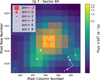 |
Fig. 1 TESS TPF of GJ7 (sector 69). The red boxes represent the aperture mask used to extract the photometry. The white cross on top of the largest red circle illustrates the position of GJ7. Other red circles stand for sources of the Gaia DR3 catalog down to 8 magnitudes fainter than our target. This plot was created with the tpfplotter code (Aller et al. 2020). |
2.2 Spectroscopy
2.2.1 ESPRESSO
GJ7 was observed with the Echelle SPectrograph for Rocky Exoplanets and Stable Spectroscopic Observations (ESPRESSO, Pepe et al. 2021) on 87 different occasions over a total of ≈2.5 yr. In this period, ESPRESSO had two technical interventions: the fiber-link was replaced in June 2019 and the replacement of a calibration lamp occurred immediately after the CoVID-19 startup in mid-December 2020. The former intervention resulted in an increased throughput. We expected the impact to be very small in the RV measurements, particularly for the calibration lamp change. However, for safety, we considered a RV offset between the data taken before and after each intervention. The first ESPRESSO data before the fiber-link upgrade (ESPRESSO18) has five observations between May 21 and June 08, 2019, the second ESPRESSO set of data (ESPRESSO19) between the first and second interventions has 37 observations between July 04, 2019, and January 31, 2020, and the third ESPRESSO group of spectra (ESPRESSO21) has 45 observations between May 14 and December 07, 2021. Out of the total of 87 spectra, 63 are new and were acquired as part of one of the ESPRESSO guaranteed time observations (GTO) subprograms dedicated to the RV follow-up to TESS and Kepler’s second light K2 mission smallsize planetary candidates (<2 R⊕). The other 24 spectra were taken under the European Southern Observatory (ESO) opentime program-id 0103.C-0849 (PI. Astudillo-Defru) and were presented in Fig. 4 by Oddo et al. (2023). When folded in phase with the planetary orbital period, the ESPRESSO data of Oddo et al. (2023) cover less than a quarter of the planetary orbit and are therefore insufficient to determine a robust planetary mass and set a constraint on the orbital ellipticity for GJ7 b.
ESPRESSO is a high-resolution, fiber-fed spectrograph that sends the spectra through two different camera arms, a red and a blue one, onto two distinct detectors covering from 378.2 through 788.2 nm with no gaps in one single shot. It is installed in a temperature and pressure-controlled, vacuum chamber at the Very Large Telescope (VLT) on the Cerro Paranal Observatory (Chile). We used any of the four units of the VLT, the 1″fiber, the high resolution (HR) mode, and a 2×1 binning on the detectors (pixel projection on the sky of 0.″041), all of which yield optical spectra with a resolving power of ≈138 000. The typical exposure time per observing epoch was 900 s or 1200 s, depending on the seeing conditions and observing program. The target was always centered on fiber A while fiber B, which is located at 7″ from fiber A, was used to register the sky background contribution, which was later used during the data reduction process. Given that the faint nature of GJ7 at blue wavelengths, no wavelength calibration source was taken simultaneously on fiber B to avoid any possible photon contamination in the data. This leads to a worse RV precision than the usual ESPRESSO RV accuracy. On average, the S/N of the spectra ranges from 35 to 89 at 550 nm, only the very first observation has a lower S/N of 27 because it was acquired under rather poor conditions of sky transparency. The remaining data were obtained typically with a seeing ≤1.″5 and air masses ≤2.0. The typical seasonal cadence consisted of one RV measurement every few to several days, with occasional nights featuring two measurements. No night binning was applied.
All ESPRESSO raw data were processed with the dedicated pipeline (version 3.0.0 of the data reduction software, DRS) that produces “science-ready” products including (i) wavelength- calibrated spectra corrected for hot pixels, cosmic rays, bias, flat-field, blaze angle, and instrumental response, (ii) the crosscorrelation functions (CCFs) generated by using an M0 spectral type mask, (iii) accurate RVs of the star corrected for the barycentric velocities, and (iv) measurements of various spectral indices that are highly useful to monitor the stellar activity. For a better description of the workflow of the ESPRESSO data reduction pipeline, we refer to Pepe et al. (2021). The CCFs were fit with Gaussian functions to determine the full-width- at-half-maximum (FWHM), the contrast indices, and the RVs (e.g., Baranne et al. 1996). The uncertainties associated with the measured RVs are computed using the algorithms described in Bouchy et al. (2001), which are valid for measurements close to the limit given by photon noise. In this work, we reduced the GTO and Oddo et al. (2023) data in the same manner for consistency. The average error bar of the ESPRESSO individual RVs is 1.13 ms−1 with an associated root mean square (rms) of 0.42 m s−1. This contrasts with the larger dispersion of the RV measurements of 2.87 m s−1. Among the spectral indices, besides the CCF parameters, we also used in this study the bisector velocity span index (BIS, Queloz et al. 2001), the depth of Hα, the depth of sodium doublet (NaD, Díaz et al. 2007), and the Ca II log  indices (Noyes et al. 1984; Lovis et al. 2011; Suárez Mascareño et al. 2015). The DRS also provides the chromospheric Ca II S -index (Noyes et al. 1984). However, we checked that it follows after log
  and thus decided to employ the latter. The whole set of ESPRESSO DRS RVs can be found in Table A.1, while the spectral indices are given in Table A.2 in the Appendix. The considerable gap of about 469 d in the ESPRESSO time series between ESPRESSO19 and ESPRESSO21 coincides with the suspension of science operations at Cerro Paranal Observatory due to the situation caused by the CoVID-19 pandemic and the time needed by the Observatory staff to start up the instrument.
The ESPRESSO DRS RVs were obtained via crosscorrelating the individual spectra against a mask containing the expected position of stellar absorption lines built for the same spectral type as our target (M0) and fitting the resulting CCFs with Gaussian profiles. The mask has different weights for different lines. For M dwarfs, rich in molecular bands, it is also customary to extract the RVs through maximum-likelihood optimization against a high S/N template created by co-adding all available observed spectra of the star (e.g., Howarth et al. 1997), the so-called template-matching technique. A few templatematching implementations are available in the literature (e.g., HARPS-TERRA, Anglada-Escudé & Butler 2012; NAIRA, Astudillo-Defru et al. 2017b; SERVAL, Zechmeister et al. 2018; WOBBLE, Bedell et al. 2019; and SBART, Silva et al. 2022). We used SERVAL to obtain the template-matching RVs of GJ7; the results are given in Table A.1. These measurements have a dispersion of 2.63 ms−1 (only slightly smaller than the ESPRESSO DRS RV dispersion) and a mean error bar of 0.52 ms−1 with an rms of 0.17 ms−1. Because this technique provides RV measurements with associated error bars twice as small as those of the DRS, we employed ESPRESSO SERVAL velocities in what follows.
2.2.2 HARPS
GJ7 was also observed with the High Accuracy Radial Velocity Planets Searcher (HARPS, Mayor et al. 2003) by Astudillo-Defru et al. (2017a) on 11 different occasions over a period of eight days between October 23 and 31, 2007, that is about 12 years before the ESPRESSO campaigns. The HARPS data were used to study the magnetic activity of the star and were not intended to search for planets. Although HARPS RVs were tabulated by Astudillo-Defru et al. (2017a) and Trifonov et al. (2020), we downloaded the HARPS measurements from the Data and Analysis Center for Exoplanets3 database (DACE, Buchschacher et al. 2020), which were obtained from the reduced spectra with the HARPS pipeline version 3.5 and following the crosscorrelation technique. Note that this technique is much more robust for deriving accurate RVs than the template-matching algorithm when the number of available spectra is small. Out of the 11 observations, one was rejected due to a very low quality of the spectrum. The mean error bar of the remaining 10 HARPS RVs in Table A.3 is 4.3 ms−1, about four times larger than that of ESPRESSO (also using the cross-correlation method). The velocity dispersion is 3.8 ms−1, roughly 1 ms−1 higher. It is unclear whether this increased dispersion reflects a more active stellar state in October 2007 or simply results from the larger measurement uncertainties. Due to the limited number of HARPS observations, the large time gap with ESPRESSO data, and their high uncertainties, which give them reduced weight, we excluded the HARPS data from the planetary system analysis in Section 4.
3 Stellar parameters of GJ7 (TOI-198)
3.1 Luminosity, mass, and radius
GJ7 was included in the Radial Velocity Experiment (RAVE, Steinmetz et al. 2020), a magnitude-limited spectroscopic survey of Galactic stars randomly selected in the Southern Hemisphere. However, the reported stellar temperature, surface gravity, and stellar metallicity are strongly discrepant by 3000 K (temperature), a factor of about 1500 (surface gravity), and 0.5 dex (metallicity). This discrepancy is likely due to the fact that our target is near the bright edge of the magnitude range studied in RAVE. GJ7 is actually listed in the catalogs of bright M dwarfs by Lépine & Gaidos (2011) and Frith et al. (2013). We decided to obtain our own stellar parameters using ESPRESSO spectra and all photometry available in the literature.
All ESPRESSO data were combined to produce a high S/N spectrum of GJ7, which was used to derive the stellar parameters (effective temperature – Teff, surface gravity — log g∗, and metallicity – [Fe/H]) of GJ7 by means of the STEPARSyN4 code (Tabernero et al. 2022), a Bayesian spectral synthesis implementation particularly designed to infer the stellar atmospheric parameters of late-type stars following a Markov chain Monte Carlo approach. The complete list of atomic and molecular lines and the grid of model atmospheres employed by STEPARSyN are described in Marfil et al. (2021). We obtained log g∗ = 4.71 ± 0.13 (cms−2), [Fe/H] = −0.66 ± 0.10 dex, and Teff = 3801 ± 32 K. The derived temperature agrees with the expectations for main-sequence M0-type dwarfs (e.g., Rajpurohit et al. 2013). We artificially increased the temperature uncertainty to ±100 K to account for possible systematics because, as described by Marfil et al. (2021), variations of this typical size are seen among the results for the same M-type stars when using different model atmospheres, atomic and molecular data, and radiative transfer code. As an example, we also employed the machine learning tool ODUSSEAS (Antoniadis-Karnavas et al. 2020) based on the measurement of the pseudo equivalent widths of more than 4000 stellar absorption lines to determine the stellar Teff and metallicity, obtaining Teff = 3649 ±94 K and [Fe/H] = −0.43 ± 0.12 dex. Both sets of measurements are compatible at the 2σ level. Interestingly, the atmosphere of GJ7 was also found to be slightly metal-depleted by other groups employing independent data; for example, Kuznetsov et al. (2019) derived [Fe/H] to be between −0.36 and −0.90 dex from HARPS spectra, and Gaidos et al. (2014) measured [Fe/H] = −0.38 dex and Teff = 3735 K from lower resolution spectra. Our adopted stellar parameters are summarized in Table 1.
According to various optical and infrared color–metallicity relations established for a thousand M0–M5 dwarfs by Duque-Arribas et al. (2023), based on Bayesian statistics and Markov chain Monte Carlo techniques, GJ7 has [Fe/H] = −0.64 ± 0.16 dex considering the W1–W2 and the Gaia Bp–Rp colors along the absolute Gaia magnitude. We caution that the Duque-Arribas et al. (2023) work is limited to the interval −0.45 ≤ [Fe/H] ≤ +0.45 dex. The photometric data of GJ7 suggests an iron abundance below the lower limit of this study, which agrees with the spectroscopic results. Several color–magnitude diagrams were produced and are shown in Fig. 2. GJ7 occupies a subluminous position with respect to the solar-metallicity main sequence of field M dwarfs. To build the diagrams, we employed Gaia data release 3 (DR3) photometry and parallax (Gaia Collaboration 2016, 2022) and 2 μm All Sky Survey (2MASS, Skrutskie et al. 2006) data. Figure 2 also displays the location of well-known metal-depleted early- to mid-M dwarfs with metallicities [Fe/H] ≤ −1 dex from the catalog of Leggett et al. (2000). GJ7 lies between the solar-metallicity main sequence and low-metallicity stars, well separated from the young stars of Group 29 (Oh et al. 2017; Luhman 2018), supporting the subsolar metallicity inferred from the ESPRESSO spectrum.
We determined the photometric spectral energy distribution (SED) of GJ7 (TOI-198) illustrated in Fig. 3 by combining all broad-band photometry available from public archives: the Galaxy Evolution Explorer (GALEX, Bianchi et al. 2017) providing near-ultraviolet data, optical photometry from the American Association of Variable Star Observers Photometric All-Sky Survey (APASS, Henden & Munari 2014), the Tycho-2 catalog (Høg et al. 2000), the Catalog of Homogeneous Means in the UBV System (Mermilliod 1997), the Gaia DR3 archive (Gaia Collaboration 2016, 2022), the Sloan Digital Sky Survey (York et al. 2000), near-infrared photometry from 2MASS (Skrutskie et al. 2006), the Deep Near-Infrared Survey of the Southern Sky database (DENIS, Epchtein et al. 1999), and mid-infrared data from the Wide-field Infrared Survey Explorer (WISE, Wright et al. 2010). Observed magnitudes were converted into fluxes by using the zero points given in the Virtual Observatory SED Analyzer tool (VOSA, Bayo et al. 2008), and observed fluxes were transformed into absolute fluxes by employing the Gaia DR3 trigonometric parallax. GJ7’s SED covers wavelengths from ≈0.25 through ≈25 μm. The PHOENIX solar-metallicity model (Husser et al. 2013) with Teff = 3800 K and log g∗ = 5.0 (cm s–2) yields a good match to the photometric observations (see Fig. 3). The steps of these models are 100 K in temperature and 0.5 dex in surface gravity. The photometric results are thus fully compatible with the spectroscopic determinations. At very short wavelengths, GJ7 shows higher fluxes than expected from purely photometric emission, which is a clear signpost of stellar activity. At long wavelengths, there is no evidence of infrared flux excesses up to ≈25 μm. Therefore, GJ7 does not appear to host a warm debris disk.
The stellar bolometric luminosity was obtained by integrating the observed SED (GALEX data, which have a non- photospheric origin in GJ7, were excluded from the integration). The trapezoidal rule was used for approximating the integral. We did not complete the photometric SED below 0.25 μm and above 25 μm because these fluxes contribute less than 1% to the total luminosity for temperatures such as that of GJ7. In addition, this little contribution is typically smaller than the quoted error bar. We obtained L = 0.0328 ± 0.0010 L⊙, where the uncertainty accounts for the errors in distance and all photometry. As a consistency check, the left panel of Fig. 4 was produced where bolometric luminosity is plotted against temperature for field M-type stars of different metallicity: solar abundance stars come from the catalog of Schweitzer et al. (2019) and low- metallicity stars from Kesseli et al. (2019). All stars depicted in Fig. 4 have their temperatures and luminosities measured in a fashion similar to that of GJ7, i.e., Teff values were computed from spectral analysis, and bolometric luminosities were obtained from the integration of the stellar SEDs. The 5 Gyr isochrones taken from the BT-Settl models of Allard et al. (2013) with [Fe/H] between solar and –2 dex are included in Fig. 4. GJ7’s location in the Hertzsprung-Russell diagram is well reproduced by the model with [Fe/H] = –0.5 dex, which agrees with our metallicity derivation using the ESPRESSO spectrum within the quoted errors. Both optical and near-infrared photometry and optical spectroscopy indicate that GJ7 is a star with a small, but measurable, subsolar metallicity.
The star’s radius (R∗) follows the Stefan-Boltzmann law, which states that the radiant thermal energy emitted from a blackbody is directly proportional to the fourth power of its temperature. The stellar luminosity is the total power radiated by the star (approximated by a blackbody); hence,  , where σSB is the Stefan-Boltzmann constant. By using the bolometric luminosity and the spectroscopically derived temperature, we obtained R∗ = 0.418 ± 0.029 R⊙ for GJ7, where the quoted error bar accounts for the luminosity and Teff uncertainties. We measured the stellar mass, M∗, by using the mass-radius relation of Schweitzer et al. (2019, their equation 6), which is based on the compilation of 55 detached, double-lined, doubleeclipsing, main-sequence M dwarf binaries from the literature (young dwarfs were excluded), obtaining M∗ = 0.417 ± 0.045 M⊙, where the error bar is the sum of the dispersion of the empirical relation and the uncertainty directly derived from the error in the stellar radius. The mass of GJ7 can also be independently estimated from the K-band-mass relation given in Mann et al. (2019), based on the analysis of 62 nearby binaries. We obtained M∗ = 0.444 ± 0.024 M⊙, a value that is fully compatible at the 1σ level with our previous derivation. In a conservative approach, we adopted the mass with the larger error bar for the following two reasons: due to the way in which it was obtained, it incorporates all the information of the stellar SED, contrasting with the mass with a small error based only on the K-band luminosity, and a larger error bar considers the dispersion of various stellar mass measurements by different methods, including the comparison with evolution models (see below).
The adopted mass and radius of GJ7 are provided in Table 1 together with the stellar surface gravity directly derived from these parameters, log g∗ = 4.81 ± 0.10 (cm s–2). The agreement at the 1σ level between the spectroscopically derived and luminosity-based log g∗ values adds support to the determination of the stellar parameters of GJ7. We remark that the Schweitzer et al. (2019) relation is valid for solar-metallicity stars. The right panel of Fig. 4 displays the stellar radius against atmospheric metallicity for field M dwarfs. Overplotted are the BT-Settl models of Allard et al. (2013) for different stellar masses between 0.09 and 0.6 M⊙ and a fixed age of 5 Gyr. As shown by the theory, both the stellar mass and the radius become smaller with decreasing metallicity by ≈6% (mass) and ≈3% (radius) for [Fe/H] between solar and −1 dex, masses in the interval 0.25–0.6 M⊙, and ages of Gyr. Although these values are on the order of the quoted mass and radius uncertainties, we decided not to apply any correction to the stellar mass derivation of GJ7 because our target, albeit slightly metal poor, still has a nearsolar metallicity. The radius does not require any correction since it was determined directly from the stellar SED. We highlight that our adopted mass, independent of any evolutionary model, is consistent at the 1σ level with the mass inferred (≈0.45 M⊙) from the BT-Settl models shown in Fig. 4.
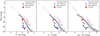 |
Fig. 2 Color-magnitude diagrams displaying the location of GJ7 (TOI-198), the young stellar sequence of Group 29 (Oh et al. 2017; Luhman 2018), the main sequence of M-type stars (Cifuentes et al. 2020), and several confirmed low-metallicity field stars with spectral types M1–M6 from the catalog of Leggett et al. (2000). The dispersion of the main sequence is shown by the gray-shaded area. |
Stellar parameters.
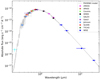 |
Fig. 3 Photometric spectral energy distribution of GJ7 (circles). The PHOENIX solar-metallicity model (Teff = 3800 K, log g∗ = 5.0 cm s−2) is shown by the gray line normalized to the observed fluxes between 0.8 and 1.6 μm (Husser et al. 2013). Photometric error bars are included, although for most of the wavelengths they have the size of the symbol. The horizontal errors account for the effective width of the filters. At short wavelengths, GJ7 exhibits flux excesses with respect to the photospheric emission indicative of some stellar activity, while at the longest wavelengths, there are no obvious infrared flux excesses. Both axes are on a logarithmic scale. |
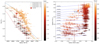 |
Fig. 4 (Left panel): Hertzsprung–Russel diagram of field M-type stars with different metallicities. GJ7 (TOI-198) is depicted by the star symbol. Solar-metallicity stars come from Schweitzer et al. (2019) and low-metallicity stars were collected from Kesseli et al. (2019). Stellar metallicity is color-coded. The 5 Gyr isochrones of the BT-Settl models ([Fe/H] between solar and –2 dex produced by Allard et al. (2013) are depicted by the solid lines. (Right panel): stellar radius versus metallicity. Tracks of constant mass (Allard et al. 2013) are shown by the blue lines. Stellar Teff is color-coded. The stellar radius axis is on a logarithmic scale. |
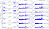 |
Fig. 5 Left: ESPRESSO data (blue dots) and their linear trend (green line). Middle and right columns: GLS periodograms of the original data and data corrected for the linear trend. The vertical red line stands for the orbital period of the transiting planet GJ7 b, while the pink band indicates the most likely rotation period of the parent star. The 0.1%, 5%, and 10% FAP levels are plotted with horizontal orange lines. |
3.2 Rotation period
The rotation period of GJ7 was addressed in the literature by Astudillo-Defru et al. (2017a). These authors employed existing HARPS data of GJ7 to estimate a rotation period of 46 ± 8 d through the Prot—log RHK relationship for M dwarf stars newly derived in their paper. The rotation-activity relation by Suárez Mascareño et al. (2018) predicts a slower rotation period of 62 ± 7 d given the ESPRESSO chromospheric activity level of GJ7 and an amplitude signal between 1 and 2 m s−1 in the RV time series caused by stellar variability.
We used the ESPRESSO activity indicators to measure the true rotation period of the star. In particular, the ESPRESSO CCF FWHM parameter has been used as a reliable indicator of stellar activity (Suárez Mascareño et al. 2020, 2023; Lillo-Box et al. 2021; Faria et al. 2022), although the values of coherence timescale for various activity indicators, including RV, do not always converge to a unique quantity (Barros et al. 2022). Figure 5 (second through seventh panels) shows all of the spectral activity indicators (left column) and their generalized Lomb- Scargle (GLS) periodograms (Zechmeister & Kürster 2009) built between 1.5 and 1500 d (middle column). Because some indices have a linear trend (possibly indicating long-term variability or a cycle of the star), we also computed the GLS periodograms after subtracting a straight line from the original data (right column panels of Fig. 5). With the exception of the Hα index, all indices manifest a forest of peaks between 42 and 56 d, which is above the 0.1% false alarm probability (FAP), that is statistically significant for the CCF FWHM and contrast, log RHK and Na indicators. We attributed this cyclic signal to GJ7’s rotation period. The control bands used to compute the Hα index contain telluric contributions that can introduce undesirable variations, thereby preventing a reliable measurement of the stellar variability.
To better quantify the stellar rotation period and its associated uncertainty, we followed two procedures: the centroid determination of the highest peak of the GLS periodograms after subtraction of the linear trend from the data and a cyclic function fit to the ESPRESSO CCF FWHM observations. Both methods actually converged to the same result. From the periodograms of Fig. 5 produced with the GLS algorithm of the pyAstronomy package (Czesla et al. 2019), we obtained Prot = 47.23 ± 0.15 d (CCF FWHM), 49.90 ± 0.20 d (CCF contrast), 49.86 ± 0.27 d (Na), 49.85 ± 0.18 d (log RHK), and 50.01 ± 0.18 d (differential line width). Following the standard pre-whitening procedure, we removed these strong signals from the datasets by finding the best-fitting amplitude and phase of a sine function with these periodicities and subtracting them from the original indices. We then recalculated the GLS periodograms of the modified data, finding no additional significant peaks with FAP < 0.1%.
For fitting (multiple) sine function(s), we employed the juliet5 tool (Espinoza et al. 2019), which provides nested sampling algorithms allowing a thorough sampling of the parameter space, and performed model comparison via Bayesian evidences. The free parameters are the amplitudes, periods, and phases of the sine waves. We accounted for the large-scale variations of the stellar activity indices by fitting a long-term trend in addition to the sinusoidal model, all of which are fit together. A jitter term was also considered and added in quadrature to the error bars. Uninformative priors were set on all of the parameters (e.g., the rotation period was sampled in the interval 10–100 d), except for the jitter that has a log-uniform prior. We tried models with one (Prot) and two (Prot and Prot/2) sine waves and two different functionals accounting for the long-term trend: polynomials of orders 1 (straight line) and 2 (parabola). We employed a dynamic nested sampling that is implemented in dynesty6 (Speagle 2020), which is recommended for simulations with a large parameter space. To compare the various models, we used the Bayesian log-evidence, log : the more positive the log-evidence, the more preferred the model is. Out of the four possible model combinations (one sine wave and a straight line, two sine waves and a straight line, one sine wave and a parabola, and two sine waves and a parabola), the Bayesian statistics (Trotta 2008) indicates that a single sine wave and a linear trend yield the most optimal solution (Table 2). The corner plot displaying the distribution of the posteriors is shown in Fig. A.1. The preferred model with Prot = 47.19 ± 0.13 d and the ESPRESSO CCF FWHM time series are depicted in Fig. 6. The analysis yielded a relatively high jitter of 3.4 m s−1. The CCF FWHM residuals (illustrated in the bottom panel of the Figure) have an rms = 4.25 m s−1, which is of the same order as the amplitude of the model (4.47 ± 0.64 m s−1) indicating that some more stellar variability not accounted by a simple sinusoidal function is taking place; that is the stellar variability amplitude of GJ7 is not necessarily constant from one rotation cycle to the next. We adopted the weighted mean rotation period of 48.5 ± 1.0 d, where the error bar includes the uncertainty of the rotation period determination after fitting a sine wave to the ESPRESSO CCF FWHM data, and the dispersion of the GLS peaks among the various spectral activity indicators. GJ7’s rotation period is listed in Table 1.
Log-evidence of ESPRESSO CCF FWHM fits.
3.3 Age
The age of GJ7 remains rather uncertain. From its position in the color-magnitude and Hertzsprung-Russell diagrams (Figs. 2 and 4), we could discard young ages because GJ7 is not over luminous with respect to the field sequence of M-type stars. To further reject young ages, we searched for lithium in the atmosphere of the star. Lithium is present in the atmospheres of young, low-mass stars and is rapidly depleted by nuclear reactions in the stellar interiors during the pre-main-sequence phase (Magazzù et al. 1993; Rebolo et al. 1996; Basri 2000). GJ7 neither shows lithium absorption at 6707.82 Å (position of the strong atomic resonance doublet), nor can it be distinguished from CN features absorbing at the same wavelengths, as is illustrated in the bottom panel of Fig. 7. We measured an upper limit on the lithium doublet equivalent width of ~50 mÅ. GJ7 has severely consumed its original photospheric lithium abundance. Using the empirical models of lithium equivalent width versus Teff and age (lithium chronology) of Jeffries et al. (2023, their Fig. 2), we inferred an age >50 Myr for GJ7, which fully agrees with the photometric and kinematics age constraints, although it is not very restrictive.
Additionally, we computed the transverse velocity (vt) and the Galactic space velocities components U, V, and W (given in Table 1) using Gaia DR3 proper motion, parallax, and RV, as well as the prescription of Johnson & Soderblom (1987), which includes the calculation of the space velocities error bars from the uncertainties in the observational quantities. The UVW values are in the directions of the Galactic center, Galactic rotation, and north Galactic pole, respectively. Note that the right-handed system is used and that we do not subtract the solar motion from our calculations. The obtained UVW values are compatible with those published by Reid et al. (1995) and Hawley et al. (1996), although ours have significantly smaller error bars because of the accurate Gaia DR3 distance and proper motion. From its kinematics, GJ7 does not belong to any known young stellar moving group with ages ≤800 Myr (we checked all the groups included in Gagné & Faherty 2018, their Table 1). GJ7 has a total space velocity of vtot = 81.1 ± 0.2 km s−1. Following the kinematic criteria of Nissen (2004) to group stars into the thin disk (vtot ≤ 85 km s−1), thick disk (85 < vtot ≤ 180 km s−1), or halo (vtot > 180 km s−1), GJ7 would lie at the boundary of the thin and thick disk of the Galaxy, which although including stars as old as ∼10 Gyr, has a relatively young component with an age ≥1 Gyr and metallicity close to the solar one (Caloi et al. 1999). From the age–metallicity relation of stars with transverse velocity vt < 120 km s−1 discussed in Sahlholdt et al. (2022) and Stokholm et al. (2023), it is inferred that GJ7’s age could be between 2 and 14 Gyr, with older ages having higher probability. In summary, all total space and transverse velocities indicate a kinematically mature age.
It is known that stellar activity and variability are correlated with age: the smaller the amplitude of variability, the older the star. Barber & Mann (2023) explored this relation using a newly defined excess photometric uncertainty in Gaia DR3 photometry as a proxy for variability. They found that the metrics follow a Skumanich-like relation, scaling as t−0.4, where t is time. From Equation 2 of Barber & Mann (2023) and using the predicted magnitude uncertainty for the brightness and number of Gaia observations of GJ7 in each of the three bands (Riello et al. 2021), we obtained the following excesses: VarG = 0.454 (G band), VarBp = 0.272 (Bp band), and VarRp = 0.265 (Rp band). The activity–age relations of Barber & Mann (2023) are calibrated against known stellar clusters with ages < 2.6 Gyr and are valid for stars with spectral types between A0 and M5 and photometric excesses greater than 0.4. Therefore, from the Gaia Bp and Rp data, it is inferred that GJ7 has a likely age > 2 Gyr while the G band suggests a younger age of  Gyr.
Gyr.
GJ7 shows broad Ca II H and K pho−tospheric absorption lines with considerable structure (top panel of Fig. 7). There is strong chromospheric emission with a weak central absorption in both Ca II lines. The latter likely stems from the dependence of the source function on height in the optically thick chromosphere rather than from actual absorption (Rauscher & Marcy 2006). From the ESPRESSO data, we measured an average index of log RHK = −5.355 dex with a standard deviation of 0.054 dex. The age-RHK relation of Wright et al. (2004, their Equation 15) yields an age of 16 ± 2 Gyr, which we interpreted as GJ7 potentially being as old as the Galactic disk (≈10 Gyr).
We also used the well-established gyrochronology method, the application of relations between stellar rotation and age (e.g., see Barnes 2007), for dating GJ7. Stellar rotation provides a potential age diagnostic that is precise, simple, and applicable to a broad range of low-mass stars. The equatorial rotation period of GJ7 was measured at Prot = 48.5 ± 1 d (see previous section). Using Fig. 11 of Shan et al. (2024) and Fig. 1 of Newton et al. (2016), both of which illustrate well-measured rotation rates as a function of stellar mass, GJ7 lies among the slowest early-M stars of similar mass. This hints at old ages. Recently, various groups (e.g., Rebull et al. 2017; Agüeros et al. 2018; Curtis et al. 2019, 2020; Douglas et al. 2019; Pass et al. 2022; Dungee et al. 2022) have produced empirical gyrochrones, that is tracks displaying the distribution of the measured rotation periods of confirmed stellar members of open clusters as a function of stellar mass (or any other proxy, e.g., color or Teff). So far, these observationally constructed gyrochrones are available in the literature from very young ages (tens of megayears) up to 4 Gyr (Gaidos et al. 2023). The equatorial rotation period of GJ7 is significantly slower by ≈20 d than the median rotation of 3800-K stars of the 4 Gyr old M67 cluster (Dungee et al. 2022), as illustrated in Fig. 8. This result implies that GJ7 is likely older than 4 Gyr. Given the uncertainties, metallicity may not be a major issue because both our target and M67 stars have nearsolar values. Nevertheless, following the analysis by Gaidos et al. (2023), the correction to be applied to the stellar gyrochronology age estimate of GJ7 is on the order of 1 Gyr, which clearly has no impact in our study. Furthermore, according to the study by Bouma et al. (2023), an age uncertainty between 10% and 50% over the first Gyr is expected for low-mass stars and the gyrochronology method; this error is typically larger than any possible correction due to a lower metallicity.
By applying the Skumanich-type spin-down relation t = t0 × (Prot/P0)1/0.62 (Gaidos et al. 2023), where t0 = 4 Gyr and P0 = 28.4 d for Teff = 3800 K stars, we derived a likely age of 9 to 10 Gyr for GJ7. However, a closer inspection of Fig. 8 reveals that other stars of the M67 cluster and GJ7 share a similar temperature and rotation period. It is beyond the scope of this paper to investigate the quality of the M67 data and cluster membership (nonmembership is contaminating the diagram of Fig. 8). Very recently, Engle & Guinan (2023) determined age–rotation relationships for M dwarfs based on stars of known age via cluster membership and companionship to white dwarfs. Using their Eq. 1, which is valid for M0–M2 stars, we derived a likely age of  Gyr for GJ7. After considering the discussion of this section, our conservative approach is to adopt an age ≥ 1 Gyr for GJ7, which is given in Table 1.
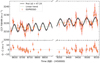 |
Fig. 6 (Top panel) ESPRESSO CCF FWHM (dots) as a function of time, along with the best sinusoidal model (black line) with a rotation period of 47.19 d (linear trend shown by the straight green line). The 1σ uncertainty of the model is depicted by the gray-shaded area. (Bottom panel) Observed minus computed diagram displaying the FWHM residuals. The derived jitter term (thin vertical line) is quadratically added to the nominal errors (thick vertical line). Stellar variability is reasonably well approximated by a sinusoidal function. |
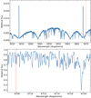 |
Fig. 7 ESPRESSO spectra around Ca II H and K and Hϵ lines (top), and lithium lines (bottom). Hϵ (in emission) and the lithium doublet wavelengths are marked by vertical red lines. The wavelength is in the air system. No clear lithium feature is observed. |
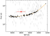 |
Fig. 8 Rotation periods of low-mass stars against Teff. GJ7 is depicted by the red star symbol. The 4 Gyr gyrochone defined in Dungee et al. (2022) is shown by the orange line. The members of the M67 cluster used to define the 4 Gyr gyrochrone are displayed by the black dots, while other cluster members are shown by gray dots. |
4 Planetary system analysis
The ESPRESSO RV time series is illustrated in the top left panel of Fig. 5. The corresponding GLS periodograms obtained for periods in the interval 1.5 to 1500 d have the highest peak at 10.2 d (FAP < 0.1%) coinciding with the planet candidate orbital period. The data folded in phase with this period show a sinusoid-like pattern, although affected by a dispersion remarkably larger (>4×) than the quoted error bars. This finding, fully independent of the photometric time series, strongly confirms the planetary nature of GJ7 b, while indicating some other additional signals hidden in the data. To reveal them, we removed the planetary signal by fitting a sine function to the data and obtained the GLS periodogram of the residuals. A second peak appears at 24.1 d with a FAP level of 1%. This agrees with half the rotation period of the parent star. In a third iteration, we recover a peak at ≈48.4 d with a FAP = 10%. This value is compatible with the stellar rotation cycle. In successive iterations, the GLS periodogram shows no significant peak above FAP = 10%. Therefore, we concluded that the information contained in the ESPRESSO RVs is dominated by the Keplerian signal at 10.218 d and the stellar activity at two preferred timescales, that of the star’s rotation period and its half value.
We combined the TESS and CHEOPS light curves and the ESPRESSO RVs to produce the most precise planetary parameters for GJ7 b. Although the TESS PDCSAP fluxes are recommended because they are corrected for instrumental issues and contamination from other sources, we decided to use the SAP fluxes for the following reasons: to the best of our knowledge there is no other source contaminating the photometric time series and one additional planetary transit is gained in sector 29 (Julian date = 2459112.299) of TESS, as shown in Fig. 9. This transit is not present in the PDCSAP data. In total, there are eight full photometric planetary transits analyzed here: seven were covered by TESS (SAP fluxes) and one full transit observed by CHEOPS.
Because the planet GJ7 b was previously validated, we employed the results of Oddo et al. (2023) to define normal priors on the orbital period and time of periastron passage of the transiting planet with Gaussian distributions. This is fully justified because these parameters are mainly constrained by the light curves, with the RV data adding little information (Kemmer et al. 2020). We removed outlier data points from the light curves by identifying the measurements deviating by more than three times the standard deviation from the median value of chunks with five points. This cleaning process was repeated once (flattened CHEOPS data) and three times (TESS SAP and PDCSAP fluxes). Less than 1.8% (SAP) and 0.5% (PDCSAP) measurements were removed. The CHEOPS data were flattened, as explained in Oddo et al. (2023). To flatten the TESS light curve, we used Gaussian process regressions (GP, Haywood et al. 2014) with an approximate Matern kernel of the form:
![Mathematical equation: ${k_i}\left( {{x_l},{x_m}} \right) = \sigma _i^2\left[ {(1 + 1/){e^{ - (1 - ){s_i}}} + (1 - 1/){e^{ - (1 + ){s_i}}}} \right],$](/articles/aa/full_html/2026/02/aa49545-24/aa49545-24-eq12.png) (1)
where
(1)
where  ,
,  , and ϵ = 0.01. The hyper-parameters ρi and σi were computed according to the celerite7 package (Foreman-Mackey et al. 2017), which provides fast calculations for large datasets. The juliet code for studying the photometric transits uses batman8 (Kreidberg 2015) for treating the transits in the light curves. The TESS and CHEOPS data were jointly modeled with a quadratic law for the stellar limbdarkening effect: we employed the parametrization q1 and q2 defined in Kipping (2013) because it is thought to reduce mutual correlations in the limb-darkening coefficients. The same values were shared by both TESS sectors. For computing q1 and q2, we used the limb-darkening coefficients derived from the Exoplanet Characterization Toolkit9 v1.2.5 by introducing the stellar parameters of Table 1 and the wavelength coverage of the TESS and CHEOPS missions. We employed the ATLAS9 model atmospheres (Kurucz 1979). The coefficients were obtained for TESS and CHEOPS separately, thus deriving q1,TESS = 0.238 ± 0.053, q1,CHEOPS = 0.402 ± 0.074, and q2,TESS = 0.159 ± 0.044, q2,CHEOPS = 0.186 ± 0.039, respectively. For a proper estimation of the error bars of the posteriors, we also set up normal priors on the stellar density, q1, and q2 parameters centered at the calculated values and with widths equal to the associated uncertainties. We also imposed log-uniform priors on the photometric jitters for the TESS and CHEOPS data, although the distribution of the posteriors suggested that the photometric jitter is negligible and has no impact on the final results. The photometric modeling of juliet includes a dilution factor per instrument, which we fixed at 1.0 because there is no nearby stellar source contributing to any of the light curves. We fit the orbital period (P) of the planet, its phase (T0), the impact parameter of the orbit (b), and the planet-to-star radius (Rp/R∗), which is directly related to the transit depth (δ = (Rp/R∗)10). In this first analysis of the light curves, we adopted a null orbital eccentricity. We fed the code with the stellar density by employing the star’s mass and radius of Table 1, which in turn served to derive the scaled semimajor axis (a/R∗) of the planetary candidate. Figure 9 shows the TESS SAP fluxes before and after being flattened. The planetary transits and the photometric GP were modeled together. Note that the photometric GP is a smooth covariance function describing both the stellar activity (particularly in sector 2) and the instrumental signatures.
The RV amplitude of the planet was obtained by simultaneously modeling two very different signals: the Keplerian wave and the stellar activity variability. We set an uninformative prior on the Keplerian amplitude with a uniform distribution. The stellar activity signal was modeled by a GP using two stochastically driven simple harmonic oscillator terms; the secondary term’s period is half the primary one. This GP, as in the celerite package, has the following power spectrum:
 (2)
where Q0 is the quality factor minus one half for the secondary oscillation (corresponding to half of the rotation), δQ is the difference between the quality factors of the first and second oscillations, f is the fractional amplitude of the secondary oscillation compared to the primary (in principle, 0 ≤ f ≤ 1), and σ is the standard deviation of the process. This rotation kernel is well suited to describing the rotation of two or more spots on different locations of the stellar surface. It was successfully used by different authors to model a range of complicated rotationally modulated signals, including wide-amplitude variations of very young stars (e.g., Winters et al. 2019; David et al. 2019; Osborn et al. 2021; Suárez Mascareño et al. 2021). We set a normal prior on Prot by adopting the rotation period of the star tabulated in Table 1. We also considered a jitter term for each of the ESPRESSO datasets together with different RV offsets. The jitter term, which was allowed to vary from a negligible value up to twice the median size of the RV error bars, was later added in quadrature to the nominal error bars of the velocities. The juliet code uses the open-source Python package radvel11 (Fulton et al. 2018) for modeling Keplerian orbits using RV data. The full set of priors is summarized in Table A.4.
(2)
where Q0 is the quality factor minus one half for the secondary oscillation (corresponding to half of the rotation), δQ is the difference between the quality factors of the first and second oscillations, f is the fractional amplitude of the secondary oscillation compared to the primary (in principle, 0 ≤ f ≤ 1), and σ is the standard deviation of the process. This rotation kernel is well suited to describing the rotation of two or more spots on different locations of the stellar surface. It was successfully used by different authors to model a range of complicated rotationally modulated signals, including wide-amplitude variations of very young stars (e.g., Winters et al. 2019; David et al. 2019; Osborn et al. 2021; Suárez Mascareño et al. 2021). We set a normal prior on Prot by adopting the rotation period of the star tabulated in Table 1. We also considered a jitter term for each of the ESPRESSO datasets together with different RV offsets. The jitter term, which was allowed to vary from a negligible value up to twice the median size of the RV error bars, was later added in quadrature to the nominal error bars of the velocities. The juliet code uses the open-source Python package radvel11 (Fulton et al. 2018) for modeling Keplerian orbits using RV data. The full set of priors is summarized in Table A.4.
From the simulations (with 500 live-points), we determined the best-fit values and their associated uncertainties for the model parameters as the median and the 0.16 and 0.84 quantiles of their posterior distributions. The three ESPRESSO RV offsets are compatible within the quoted uncertainties at the 3σ confidence level, thus suggesting no significant instrumental discontinuity induced by the technical interventions on the spectrograph. The final models indicate that the RV jitter is small. We obtained a transit depth of  ,
,  , and T0 = 2458356.37313 ± 0.00089 for a circular orbit. The relative size of GJ7 b is
  , which corresponds to a radius of 1.36 ± 0.13 R⊕ making it a super-Earth companion to GJ7. Figure 10 shows the flattened TESS and CHEOPS light curves folded in phase with the derived orbital period and mid-transit time. Our results are consistent with those of Oddo et al. (2023) but differ significantly in the determination of RV amplitude, the scaled semimajor axis and all other parameters derived from these two, including the planetary mass and transit duration T14. We computed two final models adopting circular and eccentric orbits with the goal of imposing an upper limit on the eccentricity of GJ7 b’s orbital path. The median of the posterior values for the combined photometric and spectroscopic fits are given in Table A.4. In the Appendix, Figure A.4 displays the distribution of the posteriors of the joint photometric and spectroscopic analysis (null eccentricity and TESS SAP fluxes). All distributions are reasonable. The distribution of the posteriors of the impact parameter, b, suggests that the orbital inclination angle is compatible with 90o at the 2σ confidence level.
As mentioned above, for our baseline model, we employed the TESS SAP fluxes to take advantage of the total of seven planetary transits observed by TESS. Nevertheless, for the sake of completeness, we provide the results by using the PDCSAP fluxes in Table A.5 in the Appendix. With the only obvious exception of the GP hyper-parameters of the TESS data, all fitted data are compatible with our baseline models at the 1σ the quoted uncertainties. That is, the inclusion of the photometric transit ofGJ7 b at Julian date of 2459112.299 (TESS sector 29) does not make a major impact in our analysis. We also tested different GP covariance functions to model stellar activity in the analysis. For example, we utilized the quasiperiodic kernel (Haywood et al. 2014; Rajpaul et al. 2015), of which Stock et al. (2023) concluded that modeling the stellar contribution with this kernel improves the planetary detection efficiency and leads to precise planet parameters. The results were compatible with those reported here at the 1σ level.
Table 3 provides the full set of planetary parameters obtained from the baseline models, including the fitted and derived values. Similarly, for comparison purposes, Table A.6 in the Appendix gives the planetary parameters obtained by using the TESS PDC- SAP fluxes. From our analysis and the Bayesian evidence, we concluded that both the circular and the eccentric solutions are undistinguishable. Therefore, we adopted the circular orbit solution because it has fewer variables in the simulations and imposed a 3σ upper limit of e = 0.15 on the eccentricity of GJ7 b’s orbit. Figure 11 shows the ESPRESSO RV time series together with the best fit model and the RV GP. All RV measurements with the Keplerian signal removed from the observations are folded in phase with the derived stellar rotation period at ∼48.5 d in Fig. 12. To build this figure, we used the transiting planet’s mid-transit time T0 as the phase of the modified RVs.
From the analysis, we obtained amplitudes of the GP covariance function of 2–4 ms−1, which coincide with the expectations of stellar activity-induced RV variability for GJ7 (e.g., Suárez Mascareño et al. 2018). As illustrated in Fig. 12, the peak-to-peak RV variations likely due to stellar variability is about 8 m s−1. There is a two-peak pattern in the folded, Keplerian-free RVs, although the dispersion is noticeable. This is quite likely another manifestation of the nonconstant amplitude of the stellar variability over time. The presence of additional planets may also contribute to the RV dispersion (see below).
The Keplerian signal of GJ7 b, that is the ESPRESSO RVs after subtracting the GP covariance function, folded in phase with the planetary orbital period, is displayed in Fig. 13. For completeness, we also performed the joint analysis including ESPRESSO and HARPS velocities. The results remained unchanged because the HARPS precision is insufficient to improve the planet mass determination. Figure A.2 shows all RVs folded in phase with the planetary orbital period. The rms of the ESPRESSO RV residuals is about 0.35 ms−1, which is slightly smaller than the average error bars. This indicates that the degree of overfitting of the spectroscopic data by the employed GP regression, if any, is moderate to small. Therefore, the measured Keplerian amplitude, K, is reliable. The simulations using the PDCSAP fluxes (Table A.5) provide compatible Keplerian amplitudes within the quoted uncertainties. Planet GJ7 b is robustly detected at the 7σ confidence level.
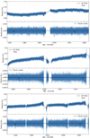 |
Fig. 9 TESS SAP fluxes of GJ7 from sectors 2 (top), 29 (middle), and 69 (bottom). Top: modeled covariance function used to flatten the data (black curves) together with the original SAP fluxes (blue points). Bottom: flattened TESS light curves (blue points) and the location of GJ7 b’s transits (black line) registered by TESS. |
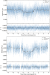 |
Fig. 10 TESS (top) and CHEOPS (bottom) data folded in phase with the planetary orbital period. The white symbols stand for binned data every 51 points (∼ 15 min, TESS) and 19 points (∼19 min, CHEOPS). The black line corresponds to the transit model. Per panel, the bottom, narrower subpanels depict the data residuals. |
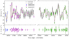 |
Fig. 11 (Top panel) ESPRESSO RV time series (dots), best-fit model (black), and GP model (brown). The gray area stands for the 1σ dispersion of the best solution. (Bottom panel) Observed minus computed residuals. |
GJ7 b (TOI-198 b) planetary parameters from the joint fit.
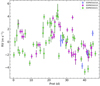 |
Fig. 12 ESPRESSO RVs folded in phase with one stellar rotation period (Keplerian signal removed). |
5 Discussion
The Rocky Worlds Director’s Discretionary Time program of the James Webb and Hubble Space Telescopes (JWST and HST) aims to search for atmospheres on rocky exoplanets orbiting M-dwarfs via secondary eclipse measurements12. GJ7 b (TOI-198 b) has been selected as a target for observations in 2026. Based on the uncertainties in Table 3, the planet’s ephemeris is expected to be accurate to within 2 minutes by mid-2026.
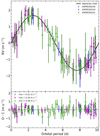 |
Fig. 13 Top panel: ESPRESSO RVs, phase-folded with GJ7 b’s orbital period after removing the stellar activity signal, along with the Kep- lerian model (black curve). Bottom panel: observed-minus-computed residuals. The planet’s mid-transit time (T0) corresponds to half an orbital period. |
5.1 Additional planets in the GJ7 system
The ESPRESSO RV data did not allow us to constrain the presence of companions (either planets or brown dwarfs) with orbital periods longer than a few years. Additionally, stellar activity and rotation usually frustrate the detection of planets using the RV method (see Newton et al. 2016). GJ7 shows variability at the timescales around the rotation period and its half-value with remarkable traces in the spectroscopic data. It is thus not possible to discern the presence of planets with orbital periods around exact multiples of the stellar rotation (e.g., ≈24, ≈48, and ≈96 d) using RV data alone.
From the ESPRESSO measurements, we may safely discard non-eccentric planets orbiting GJ7 with Keplerian amplitudes ≥9 m s−1 (three times the standard deviation of the data) and orbital periods ≤5 yr (twice the time coverage of ESPRESSO) with a high 3σ confidence. This corresponds to companion planets with masses >4 M⊕ at the shortest periods (∼0.3 d), and >60 and >95 M⊕ at ∼1 and 5 yr periods, respectively. The Gaia DR3 RUWE value (1.08) also supports the lack of massive bodies in the system based on the very small statistically significant astrometric acceleration. Figure 14 shows the upper limits at wide orbital separations from GJ7 based on the Hipparcos-Gaia proper motion anomaly as described in Kervella et al. (2022). It is inferred that companions with masses greater than 0.5 MJup are excluded in the separation range 3–10 au.
Regarding smaller orbital separations, the pre-whitening method applied to the ESPRESSO RVs (section 4) did not reveal significant signals hinting at low-amplitude periodic variability except for those attributed to GJ7 b and the stellar rotation. The fourth iteration yielded a RV GLS periodogram where the highest, insignificant peak lies at ∼5.8 d, which may suggest the presence of a second planet in a near 2:1 resonance orbit. We ran simulations to identify the 3σ upper limit on the mass of an hypothetical planet at this orbital period finding Mp ≤ 1.5 M⊕ (i.e., K ≤ 1 m s−1). Further high-precision RV measurements are needed to confirm or reject the 5.8 d signal.
However, if the 5.8 d planet candidate existed and its mass and size were similar to those of GJ7 b, it would be moving around in a non-transiting orbit based on the TESS data. That is, either the putative planet candidate would be smaller in size than GJ7 b, the candidate and GJ7 b would be in misaligned orbits (see, e.g., Bourrier et al. 2021), or both scenarios might occur simultaneously. We ran the box-fitting least squares (BLS) algorithm (Kovács et al. 2002) for the detection of additional periodically transiting planets in the TESS light curve (PDCSAP fluxes). The method is based on a simplified box-shaped model of a strictly periodic transit in which the light curve is phase- folded according to each trial period and binned in phase. We searched for planets with tentative orbital periods between 0.2 and 20 d. In the first iteration, we found the confirmed transiting planet GJ7 b at 10.2 d. The transits were then removed from the time series, and in successive iterations of the BLS algorithm, no other transiting candidate was identified. Considering that GJ7 b’s transit is detected with a significance of 8 σ in the TESS data, we quite likely missed photometric transit features with depths smaller than ≈400 ppm should they have occurred several times during the TESS observations. That is, our photometric data are not sensitive to transiting planets smaller than ≈0.9 R⊕ (size of Venus). For such small planets, the planetary mass–radius relation provided by the pure iron track of Zeng et al. (2019) (ultradense planets) can be used to establish the minimum detectable mass. In our case, this minimum mass is 1.3 M⊕.
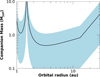 |
Fig. 14 Hipparchos-Gaia proper motion acceleration sensitivity to companions of a given mass (in Jupiter masses) as a function of the orbital semimajor axis (in astronomical units) orbiting GJ7. The solid line denotes the combinations of mass and separation explaining the observed proper motion acceleration at the mean epoch of Gaia DR3, based on the analytical formulation of Kervella et al. (2019) and the observed astrometric acceleration for GJ7 reported by Kervella et al. (2022). The shaded light blue region corresponds to the 1σ uncertainty domain. Both axes are plotted on a logarithmic scale. |
5.2 Metallicity and internal structure of GJ7 b
The super-Earth GJ7 b has a mass of  and is moving around its slightly metal-depleted parent star at a separation of
  au in a circular orbit. The planetary mass error budget is dominated by the uncertainty of the host star’s mass. GJ7 b falls into the category of small, close-in orbit planets. In what follows, we place GJ7 b in context with other known planets. Early studies (e.g., Santos et al. 2004; Fischer & Valenti 2005) established that there is a correlation between the presence of giant planets and the metallicity of their host stars. Massive planets tend to be more frequent around metal-rich stars. This qualitatively supports core accretion models where planets form by the accumulation of dust and ice particles (Ida & Lin 2004) because metals are required for cooling down protoplanetary disks. Recent simulations by pebble accretion (e.g., Nielsen et al. 2023) indicate that the masses of the planets increase on average with increasing stellar metallicity. This correlation was claimed not to be clear for planets smaller than Neptune, that is Rp ≤ 4 R⊕ (Sousa et al. 2008). However, more recent studies (e.g., Adibekyan et al. 2012; Buchhave et al. 2012; Sousa et al. 2019; Zhu 2019; Lu et al. 2020, and references therein) tend to indicate that small planets also seem to present a possible correlation in the stellar metallicity–period–planetary mass diagram where the mass of the planet increases with both stellar metallicity and orbital period. One important conclusion is that small planets form around host stars with a wide range of metallicities, but on average a metallicity close to solar (Buchhave et al. 2012). Figure 15 shows the distribution of planetary radius and density as a function of the metallicity of the host stars. More than 1000 planets with the required information available at the NASA Exoplanet Archive database13 are included. GJ7 b stands out as the planet around one of the most metal-poor parent stars. As illustrated in the bottom panel of Figure 15, where planetary density is shown, GJ7 b extrapolates the still not-so-well-populated tail of low-mass planets toward lower iron abundances, thus supporting Buchhave et al. (2012) statement that terrestrial planets may be formed with no special requirement of enhanced metallicity and challenging models that predict that short-period planets smaller than 2 R⊕ should be rare around early-M dwarfs with metallicity below −0.5 dex (Lu et al. 2020).
Because planets and stars form by accreting material from a surrounding disk, it is reasonable to assume a relationship between their compositions. Adibekyan et al. (2021) studied the iron-to-silicon mass fraction of rocky exoplanets from their masses and radii and compared them with the iron abundance of their host stars, finding a correlation, which they attributed to planet formation processes. To explore the possible impact of the low metallicity in the internal structure of GJ7 b, we built the top panel of Figure 16, where planetary mass is plotted against planetary radius. Only planets with mass and radius constrained to better than 12% are depicted for clarity: data were downloaded from the NASA Exoplanet Archive database and include the mass and radius revision of low-mass planets made by Toledo-Padrón et al. (2020), Luque & Pallé (2022), Lavie et al. (2023), Goffo et al. (2023), and Cadieux et al. (2024). The Figure also includes three interior models produced by Zeng et al. (2019): planetary cores made of pure iron (very high density planets), Earth-like rocky cores (32.5% Fe and 67.5% MgSiO3 by mass), and pure water ice. GJ7 b lies very close to the rocky model and nicely follows the narrow sequence delineated by other planets whose positions are well reproduced by the Earth-like track. In fact, the region around the GJ7 b’s position in the mass–radius diagram of Figure 16 is becoming more and more populated with the advent of powerful RV instruments. However, the dispersion of the small planets’ loci (Rp < 1.8 R⊕) with accurate mass and radius determinations remains small and hints at the fact that all of these rocky planets share a similar internal structure as that of the Earth independently of their different bulk planetary densities and iron abundances of their parent stars (Caballero et al. 2022). If the precision with which planetary radii and masses are known were relaxed by a factor of two, the dispersion would increase potentially leading to the appearance of populations of less dense super-Earths (see Castro-González et al. 2023).
Among the rocky planets, there is one outlier in the top panel of Fig. 16: GJ 367 b, an ultradense planet with a pure iron core that belongs to the super-Mercury category according to Lam et al. (2021) and Goffo et al. (2023). Interestingly, the metallicity of GJ 367 (M3-type star) is solar ([Fe/H] = −0.01 ± 0.12 dex). Therefore, metallicity cannot be the key factor to explain the different bulk densities and internal structure between GJ367 b and, for example, GJ7 b. GJ 367 b is, however, an ultrashort period planet with an orbital period of 7.7 h and an orbital path approximately ten times closer to its parent star than GJ7 b. GJ 367 b might have experienced mantle-stripping giant impacts as it has traditionally been used to explain Mercury’s high core fraction. Recent models, however, can explain these superdense planets by the direct consequence of temperature fluctuations and chemical differentiation in protoplanetary disks (e.g., Johansen & Dorn 2022).
Planet LTT 1445 A b (Winters et al. 2019; Lavie et al. 2023) appears to be less dense than Earth, indicating the presence of a water-rich atmosphere or alternatively a lower iron-mass fraction. The parent star has a slightly low metallicity, similarly to GJ7. Interestingly, LTT 1445 A b’s location is compatible with the theoretical Earth-like composition at 2σ. The planetary mass and radius of LTT 1445 A b shown in Fig. 16 are the most recent ones calculated by Lavie et al. (2023). However, the earlier measurements from Winters et al. (2021) bring the planet next to the Earth-like model in much better agreement with GJ7 b. It seems that the uncertainties associated with the determination of the planetary parameters of LTT 1445 A b are still large. Although chemical abundance is expected to have an impact on the composition of the planets, the top panel of Fig. 16 shows that, with very few exceptions, the smallest planets distribute along the Earth-like model for metallicities [Fe/H] ≥ −0.6 dex. This indicates that either metallicity has little effect and/or iron oxidation in the protoplanetary disks is rather inefficient (Nielsen et al. 2023). Planetary formation and evolution mechanisms, including inward migration processes (e.g., Schlaufman et al. 2010; Lee & Chiang 2017; Pu & Lai 2019; Petrovich et al. 2019; Millholland & Spalding 2020; Venturini et al. 2020), are likely responsible for these internal structure deviations among small and low-mass planets, in agreement with the conclusions made by Luque & Pallé (2022), although these authors did not include any ultradense planet in their study.
To investigate the internal structure of GJ7 b, we performed interior modeling using the ExoMDN code (Baumeister & Tosi 2023)14. This code uses mixture density networks to infer interior compositions, modeling the planet as a four-layer structure comprising an iron core, silicate mantle, water layer, and H/He atmosphere, based on the planetary mass, radius, and equilibrium temperature. The resulting posterior distributions for the mass fraction and thickness of each layer are shown in Fig. A.3. From these results, we estimated GJ7 b’s uncompressed density to be  , computed as the sum of the densities of the core (iron), mantle (silicates), and water layers, each weighted by their respective mass fractions. Its internal structure closely resembles that of Earth: the core mass fraction is slightly higher and the mantle fraction slightly lower, contributing to the higher uncompressed density (Earth’s uncompressed density is 4.4 g cm−3), although both remain consistent with Earth’s values within the error bars.
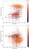 |
Fig. 15 Stellar metallicity [Fe/H] plotted against planetary radius (top) and density (bottom). Over 1000 exoplanets are plotted with their masses (on logarithmic scale) color-coded (darker implies lower planetary mass). These data are taken from the NASA Exoplanet Archive database. GJ7 b is depicted by the red point. The vertical axes are on a logarithmic scale. |
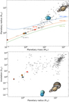 |
Fig. 16 Top: planetary mass–radius diagram, including all known exoplanets with a radius and a mass constrained to a precision better than 12% (gray, open circles). GJ7 b is depicted by the red circle. Interior models of different compositions (Zeng et al. 2019) are shown by the solid colored lines. Two other planets discussed in the text are labeled. Bottom: planetary insolation plotted as a function of planetary radius for the same planets. The eight planets of the Solar System are shown as a reference. All axes are on a logarithmic scale. |
5.3 Habitability
While GJ7 b is rocky, it is possibly not amenable for sustaining Earth-like life on its surface. The bottom panel of Figure 16 depicts the amount of stellar incident flux at the orbital separation of the planets as a function of the planetary radius. According to the models by Kopparapu et al. (2014), which present improved estimates of the boundaries of the habitable zone by updating the group’s previous work of Kopparapu et al. (2013), the habitable zone of GJ7 (where liquid water remains thermodynamically stable on the planet’s surface) lies between 0.15 and 0.36 au after computing the inner and outer edges using the “recent Venus” and maximum greenhouse limit cases. The estimates are based on water-rich planets, 1D and 3D climate models, and corresponding climate transitions that planets undergo at these limits. Although the borderline of the “recent Venus” limit case is believed to be too extreme for life (see next), the study by Yang et al. (2014) indicated that slowly rotating planets can maintain an Earth-like climate at nearly twice the incident flux the Earth receives (2× S⊕), which is actually very close to that of Venus. With an insolation ≈7× S⊕ (Table 3), similar to that of Mercury in the Solar System (see Fig. 16), GJ7 b is closer to the star than the inner edge of the habitable zone as illustrated in Fig. 17 and it is likely too warm.
We also computed the expected equilibrium temperature of the planet ( , Table 3) by adopting pure radiative equilibrium and zero Bond albedo (nonreflective planet). The error bars account for the stellar luminosity error and the uncertainty on the planetary semimajor axis. Following Equation 1 of Kempton et al. (2018), we determined the transmission spectroscopy metric (TSM) to be
  (Table 3). This quantity is proportional to the expected transmission spectroscopy S/N assuming cloud-free atmospheres and 10 h of observing time with the JWST and NIRISS instrument. The TSM is relatively small. The future ANDES spectrograph on the ELT (Palle et al. 2025) may have the necessary capabilities to explore the atmospheric properties of GJ7 b by observing and combining ∼10 planetary transits. According to Batalha et al. (2019), the mass precision achieved for GJ7 b is good enough for initial characterization of the planet’s atmosphere.
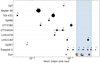 |
Fig. 17 Planetary systems containing terrestrial, transiting, low-mass exoplanets with mass Mp ≤ 4 M⊕ and radius constrained to a precision better than 12% are shown relative to the location of the estimated habitable zone (blue-shaded area, Kopparapu et al. 2014). GJ7 and the Solar System are depicted at the top and bottom, respectively. All planetary systems are scaled to GJ7. The size of the black dots is linearly scaled to the radius of the planets (excluding the Solar System). The semimajor axis errors are plotted, and the x-axis is on a logarithmic scale. |
6 Conclusions
We determined the ephemeris, along with the mass and the radius of the transiting, rocky, temperate planet GJ7 b (TOI- 198 b) using photometry from three TESS sectors, one planetary transit observation with CHEOPS, and 87 precise RV measurements obtained with ESPRESSO over 2.5 yr. There were a total of eight transits covered by TESS and CHEOPS. The results indicate that GJ7 b is a super-Earth with a mass of  and a radius of Rp = 1.36 ± 0.13 R⊕, mov- +0.0067 ing around its parent star at a separation of
  au with an orbital period of
  . The detailed photometric and spectroscopic analysis allowed us to impose a 3σ upper limit on the planetary eccentricity of e ≤ 0.15. No other transiting planet was identified down to approximately 0.9 R⊕ in the photometric light curves with tentative orbital periods between 0.2 and 20 d. While the analysis of the velocities suggested a possible second planet with an orbital period near 5.8 days and a mass lower than that of GJ7 b, the current data did not allow us to confirm it. Further RV measurements are necessary to assess the true nature of this spectroscopic signal. Although the rotation period of the M0-type planet host star is slow and constrained to be Prot = 48.5 ± 1 d, the star shows strong traces of activity with a RV amplitude of ≈4 m s−1, that is 2.5 times the Keplerian signal of GJ7 b. This hampers the detection of planets smaller than 1 M⊕ using the existing spectroscopic data.
For its mass and radius, GJ7 b lies near the Earth-like composition track in the planetary mass–radius diagram, indicating substantial similarity to Earth, whose composition is 32.5% Fe and 67.5% MgSiO3 by mass. This contrasts with the moderately low metallicity of its parent star, which was measured at [Fe/H] = −0.66 ± 0.10 dex, that is about four times less iron than the Sun. GJ7 b stands out as one of the few planets found around metal-poor stars, challenging those models predicting a halt in the formation of low-mass planets at low-metallicities. Although GJ7 b is rocky, it lies closer to its host star than the inner edge of the water-liquid-based definition of the habitable zone, rendering it unlikely to support Earth-like life on its surface. Only high albedo values would make it more favorable to life.
Acknowledgements
This research has made use of the NASA Exoplanet Archive, which is operated by the California Institute of Technology, under contract with the National Aeronautics and Space Administration under the Exoplanet Exploration Program. This research has made use of the tool provided by Gaia DPAC (https://www.cosmos.esa.int/web/gaia/dr3-software-tools) to reproduce (E)DR3 Gaia photometric uncertainties described in the GAIA- C5-TN-UB-JMC-031 technical note using data in Riello et al. (2021). We thank the anonymous referee for his/her helpful suggestions and careful reading of the manuscript. M.R.Z.O. and H.T. acknowledge funding from the Spanish Ministry for Science, Innovation and Universities through projects PID2019-109522GB-C51 and PID2022-137241NB-C42. A.S.M., J.I.G.H., and R.R. acknowledge financial support from the Spanish Ministry of Science, Innovation and Universities project PID2020-117493GB-I00 and from the Government of the Canary Islands project ProID2020010129. N.A-D. acknowledges the support of FONDECYT project 1240916. This work was supported by FCT - Fundaçâo para a Ciência e a Tecnologia through national funds and by FEDER through COMPETE2020 - Programa Operacional Competitividad e Intenacionalizaçâo by these grants: UIDB/04434/2020, UIDP/04434/2020, and 2022.04048.PTDC (Phi in the Sky, DOI 10.54499/2022.04048.PTDC). Co-funded by the European Union (ERC, FIERCE, 101052347). Views and opinions expressed are however those of the authors only and do not necessarily reflect those of the European Union or the European Research Council. Neither the European Union nor the granting authority can be held responsible for them. A.C.-G. is funded by the Spanish Ministry of Science through MCIN/AEI/10.13039/501100011033 grant PID2019-107061GB-C61. C.J.A.P.M. also acknowledges FCT and POCH/FSE (EC) support through Investigator FCT Contract 2021.01214.CEECIND/CP1658/CT0001. J.L.-B. was partly funded by grants LCF/BQ/PI20/11760023, Ramón y Cajal fellowship with code RYC2021- 031640-I, and the Spanish MCIN/AEI/10.13039/501100011033 grant PID2019- 107061GB-C61.
References
- Adibekyan, V. Z., Sousa, S. G., Santos, N. C., et al. 2012, A&A, 545, A32 [NASA ADS] [CrossRef] [EDP Sciences] [Google Scholar]
- Adibekyan, V., Dorn, C., Sousa, S. G., et al. 2021, Science, 374, 330 [NASA ADS] [CrossRef] [Google Scholar]
- Agüeros, M. A., Bowsher, E. C., Bochanski, J. J., et al. 2018, ApJ, 862, 33 [Google Scholar]
- Allard, F., Homeier, D., Freytag, B., Schaffenberger, W., & Rajpurohit, A. S. 2013, Mem. Soc. Astron. Ital. Suppl., 24, 128 [Google Scholar]
- Aller, A., Lillo-Box, J., Jones, D., Miranda, L. F., & Barceló Forteza, S. 2020, A&A, 635, A128 [NASA ADS] [CrossRef] [EDP Sciences] [Google Scholar]
- Anglada-Escudé, G., & Butler, R. P. 2012, ApJS, 200, 15 [Google Scholar]
- Antoniadis-Karnavas, A., Sousa, S. G., Delgado-Mena, E., et al. 2020, A&A, 636, A9 [NASA ADS] [CrossRef] [EDP Sciences] [Google Scholar]
- Astudillo-Defru, N., Delfosse, X., Bonfils, X., et al. 2017a, A&A, 600, A13 [NASA ADS] [CrossRef] [EDP Sciences] [Google Scholar]
- Astudillo-Defru, N., Forveille, T., Bonfils, X., et al. 2017b, A&A, 602, A88 [NASA ADS] [CrossRef] [EDP Sciences] [Google Scholar]
- Banzatti, A., Pontoppidan, K. M., Carr, J. S., et al. 2023, ApJ, 957, L22 [NASA ADS] [CrossRef] [Google Scholar]
- Baranne, A., Queloz, D., Mayor, M., et al. 1996, A&AS, 119, 373 [Google Scholar]
- Barber, M. G., & Mann, A. W. 2023, ApJ, 953, 127 [NASA ADS] [CrossRef] [Google Scholar]
- Barnes, S. A. 2007, ApJ, 669, 1167 [Google Scholar]
- Barros, S. C. C., Demangeon, O. D. S., Alibert, Y., et al. 2022, A&A, 665, A154 [NASA ADS] [CrossRef] [EDP Sciences] [Google Scholar]
- Basri, G. 2000, ARA&A, 38, 485 [Google Scholar]
- Batalha, N. E., Lewis, T., Fortney, J. J., et al. 2019, ApJ, 885, L25 [Google Scholar]
- Baumeister, P., & Tosi, N. 2023, A&A, 676, A106 [NASA ADS] [CrossRef] [EDP Sciences] [Google Scholar]
- Bayo, A., Rodrigo, C., Barrado Y Navascués, D., et al. 2008, A&A, 492, 277 [NASA ADS] [CrossRef] [EDP Sciences] [Google Scholar]
- Bedell, M., Hogg, D. W., Foreman-Mackey, D., Montet, B. T., & Luger, R. 2019, AJ, 158, 164 [Google Scholar]
- Benz, W., Broeg, C., Fortier, A., et al. 2021, Exp. Astron., 51, 109 [Google Scholar]
- Bianchi, L., Shiao, B., & Thilker, D. 2017, ApJS, 230, 24 [Google Scholar]
- Bouchy, F., Pepe, F., & Queloz, D. 2001, A&A, 374, 733 [NASA ADS] [CrossRef] [EDP Sciences] [Google Scholar]
- Bouma, L. G., Palumbo, E. K., & Hillenbrand, L. A. 2023, ApJ, 947, L3 [NASA ADS] [CrossRef] [Google Scholar]
- Bourrier, V., Lovis, C., Cretignier, M., et al. 2021, A&A, 654, A152 [NASA ADS] [CrossRef] [EDP Sciences] [Google Scholar]
- Brown, T. M., Baliber, N., Bianco, F. B., et al. 2013, PASP, 125, 1031 [Google Scholar]
- Bryson, S., Kunimoto, M., Kopparapu, R. K., et al. 2021, AJ, 161, 36 [NASA ADS] [CrossRef] [Google Scholar]
- Buchhave, L. A., Latham, D. W., Johansen, A., et al. 2012, Nature, 486, 375 [NASA ADS] [Google Scholar]
- Buchschacher, N., Alesina, F., & Ségransan, D. 2020, in Astronomical Society of the Pacific Conference Series, 522, Astronomical Data Analysis Software and Systems XXVII, eds. P. Ballester, J. Ibsen, M. Solar, & K. Shortridge, 303 [Google Scholar]
- Caballero, J. A., González-Álvarez, E., Brady, M., et al. 2022, A&A, 665, A120 [NASA ADS] [CrossRef] [EDP Sciences] [Google Scholar]
- Cadieux, C., Plotnykov, M., Doyon, R., et al. 2024, ApJ, 960, L3 [NASA ADS] [CrossRef] [Google Scholar]
- Caloi, V., Cardini, D., D’Antona, F., et al. 1999, A&A, 351, 925 [Google Scholar]
- Castro-González, A., Demangeon, O. D. S., Lillo-Box, J., et al. 2023, A&A, 675, A52 [NASA ADS] [CrossRef] [EDP Sciences] [Google Scholar]
- Cifuentes, C., Caballero, J. A., Cortés-Contreras, M., et al. 2020, A&A, 642, A115 [NASA ADS] [CrossRef] [EDP Sciences] [Google Scholar]
- Clark, C. A., van Belle, G. T., Horch, E. P., et al. 2022, AJ, 164, 33 [NASA ADS] [CrossRef] [Google Scholar]
- Curtis, J. L., Agüeros, M. A., Douglas, S. T., & Meibom, S. 2019, ApJ, 879, 49 [Google Scholar]
- Curtis, J. L., Agüeros, M. A., Matt, S. P., et al. 2020, ApJ, 904, 140 [Google Scholar]
- Czesla, S., Schröter, S., Schneider, C. P., et al. 2019, PyA: Python astronomy-related packages, Astrophysics Source Code Library [record ascl:1906.010] [Google Scholar]
- David, T. J., Petigura, E. A., Luger, R., et al. 2019, ApJ, 885, L12 [Google Scholar]
- Delrez, L., Murray, C. A., Pozuelos, F. J., et al. 2022, A&A, 667, A59 [NASA ADS] [CrossRef] [EDP Sciences] [Google Scholar]
- Demangeon, O. D. S., Zapatero Osorio, M. R., Alibert, Y., et al. 2021, A&A, 653, A41 [NASA ADS] [CrossRef] [EDP Sciences] [Google Scholar]
- Díaz, R. F., Cincunegui, C., & Mauas, P. J. D. 2007, MNRAS, 378, 1007 [Google Scholar]
- Douglas, S. T., Curtis, J. L., Agüeros, M. A., et al. 2019, ApJ, 879, 100 [Google Scholar]
- Dransfield, G., Timmermans, M., Triaud, A. H. M. J., et al. 2024, MNRAS, 527, 35 [Google Scholar]
- Dungee, R., van Saders, J., Gaidos, E., et al. 2022, ApJ, 938, 118 [NASA ADS] [CrossRef] [Google Scholar]
- Duque-Arribas, C., Montes, D., Tabernero, H. M., et al. 2023, ApJ, 944, 106 [NASA ADS] [CrossRef] [Google Scholar]
- Engle, S. G., & Guinan, E. F. 2023, ApJ, 954, L50 [NASA ADS] [CrossRef] [Google Scholar]
- Epchtein, N., Deul, E., Derriere, S., et al. 1999, A&A, 349, 236 [NASA ADS] [Google Scholar]
- Espinoza, N., Kossakowski, D., & Brahm, R. 2019, MNRAS, 490, 2262 [Google Scholar]
- Faria, J. P., Suárez Mascareño, A., Figueira, P., et al. 2022, A&A, 658, A115 [NASA ADS] [CrossRef] [EDP Sciences] [Google Scholar]
- Feliz, D. L., Plavchan, P., Bianco, S. N., et al. 2021, AJ, 161, 247 [Google Scholar]
- Fischer, D. A., & Valenti, J. 2005, ApJ, 622, 1102 [NASA ADS] [CrossRef] [Google Scholar]
- Foreman-Mackey, D., Agol, E., Ambikasaran, S., & Angus, R. 2017, AJ, 154, 220 [Google Scholar]
- Frith, J., Pinfield, D. J., Jones, H. R. A., et al. 2013, MNRAS, 435, 2161 [Google Scholar]
- Fulton, B. J., Petigura, E. A., Blunt, S., & Sinukoff, E. 2018, PASP, 130, 044504 [Google Scholar]
- Gagné, J., & Faherty, J. K. 2018, ApJ, 862, 138 [Google Scholar]
- Gaia Collaboration (Prusti, T., et al.) 2016, A&A, 595, A1 [NASA ADS] [CrossRef] [EDP Sciences] [Google Scholar]
- Gaia Collaboration (Vallenari, A., et al.) 2022, arXiv e-prints [arXiv:2208.00211] [Google Scholar]
- Gaidos, E., Mann, A. W., Lépine, S., et al. 2014, MNRAS, 443, 2561 [Google Scholar]
- Gaidos, E., Claytor, Z., Dungee, R., Ali, A., & Feiden, G. A. 2023, MNRAS, 520, 5283 [Google Scholar]
- Giacalone, S., Dressing, C. D., Jensen, E. L. N., et al. 2021, AJ, 161, 24 [Google Scholar]
- Gillon, M., Triaud, A. H. M. J., Demory, B.-O., et al. 2017, Nature, 542, 456 [NASA ADS] [CrossRef] [Google Scholar]
- Goffo, E., Gandolfi, D., Egger, J. A., et al. 2023, ApJ, 955, L3 [NASA ADS] [CrossRef] [Google Scholar]
- Hawley, S. L., Gizis, J. E., & Reid, I. N. 1996, AJ, 112, 2799 [Google Scholar]
- Haywood, R. D., Collier Cameron, A., Queloz, D., et al. 2014, MNRAS, 443, 2517 [Google Scholar]
- Henden, A., & Munari, U. 2014, Contrib. Astron. Observ. Skalnate Pleso, 43, 518 [NASA ADS] [Google Scholar]
- Høg, E., Fabricius, C., Makarov, V. V., et al. 2000, A&A, 355, L27 [Google Scholar]
- Howarth, I. D., Siebert, K. W., Hussain, G. A. J., & Prinja, R. K. 1997, MNRAS, 284, 265 [NASA ADS] [CrossRef] [Google Scholar]
- Husser, T. O., Wende-von Berg, S., Dreizler, S., et al. 2013, A&A, 553, A6 [NASA ADS] [CrossRef] [EDP Sciences] [Google Scholar]
- Ida, S., & Lin, D. N. C. 2004, ApJ, 604, 388 [Google Scholar]
- Jeffries, R. D., Jackson, R. J., Wright, N. J., et al. 2023, MNRAS, 523, 802 [NASA ADS] [CrossRef] [Google Scholar]
- Jenkins, J. M., Twicken, J. D., McCauliff, S., et al. 2016, SPIE Conf. Ser., 9913, 99133E [Google Scholar]
- Johansen, A., & Dorn, C. 2022, A&A, 662, A19 [NASA ADS] [CrossRef] [EDP Sciences] [Google Scholar]
- Johnson, D. R. H., & Soderblom, D. R. 1987, AJ, 93, 864 [Google Scholar]
- Kemmer, J., Stock, S., Kossakowski, D., et al. 2020, A&A, 642, A236 [EDP Sciences] [Google Scholar]
- Kemmer, J., Dreizler, S., Kossakowski, D., et al. 2022, A&A, 659, A17 [NASA ADS] [CrossRef] [EDP Sciences] [Google Scholar]
- Kempton, E. M. R., Bean, J. L., Louie, D. R., et al. 2018, PASP, 130, 114401 [Google Scholar]
- Kervella, P., Arenou, F., Mignard, F., & Thévenin, F. 2019, A&A, 623, A72 [NASA ADS] [CrossRef] [EDP Sciences] [Google Scholar]
- Kervella, P., Arenou, F., & Thévenin, F. 2022, A&A, 657, A7 [NASA ADS] [CrossRef] [EDP Sciences] [Google Scholar]
- Kesseli, A. Y., Kirkpatrick, J. D., Fajardo-Acosta, S. B., et al. 2019, AJ, 157, 63 [Google Scholar]
- Kipping, D. M. 2013, MNRAS, 435, 2152 [Google Scholar]
- Kopparapu, R. K., Ramirez, R., Kasting, J. F., et al. 2013, ApJ, 765, 131 [NASA ADS] [CrossRef] [Google Scholar]
- Kopparapu, R. K., Ramirez, R. M., SchottelKotte, J., et al. 2014, ApJ, 787, L29 [Google Scholar]
- Kovács, G., Zucker, S., & Mazeh, T. 2002, A&A, 391, 369 [Google Scholar]
- Kreidberg, L. 2015, PASP, 127, 1161 [Google Scholar]
- Kurucz, R. L. 1979, ApJS, 40, 1 [NASA ADS] [CrossRef] [Google Scholar]
- Kuznetsov, M. K., del Burgo, C., Pavlenko, Y. V., & Frith, J. 2019, ApJ, 878, 134 [Google Scholar]
- Lam, K. W. F., Csizmadia, S., Astudillo-Defru, N., et al. 2021, Science, 374, 1271 [NASA ADS] [CrossRef] [Google Scholar]
- Lavie, B., Bouchy, F., Lovis, C., et al. 2023, A&A, 673, A69 [NASA ADS] [CrossRef] [EDP Sciences] [Google Scholar]
- Lee, E. J., & Chiang, E. 2017, ApJ, 842, 40 [Google Scholar]
- Leggett, S. K., Allard, F., Dahn, C., et al. 2000, ApJ, 535, 965 [NASA ADS] [CrossRef] [Google Scholar]
- Lépine, S., & Gaidos, E. 2011, AJ, 142, 138 [Google Scholar]
- Lester, K. V., Matson, R. A., Howell, S. B., et al. 2021, AJ, 162, 75 [NASA ADS] [CrossRef] [Google Scholar]
- Lillo-Box, J., Figueira, P., Leleu, A., et al. 2020, A&A, 642, A121 [NASA ADS] [CrossRef] [EDP Sciences] [Google Scholar]
- Lillo-Box, J., Faria, J. P., Suárez Mascareño, A., et al. 2021, A&A, 654, A60 [NASA ADS] [CrossRef] [EDP Sciences] [Google Scholar]
- Lovis, C., Ségransan, D., Mayor, M., et al. 2011, A&A, 528, A112 [NASA ADS] [CrossRef] [EDP Sciences] [Google Scholar]
- Lu, C. X., Schlaufman, K. C., & Cheng, S. 2020, AJ, 160, 253 [Google Scholar]
- Luhman, K. L. 2018, AJ, 156, 271 [Google Scholar]
- Luque, R., & Pallé, E. 2022, Science, 377, 1211 [NASA ADS] [CrossRef] [Google Scholar]
- Magazzù, A., Martin, E. L., & Rebolo, R. 1993, ApJ, 404, L17 [NASA ADS] [CrossRef] [Google Scholar]
- Mann, A. W., Dupuy, T., Kraus, A. L., et al. 2019, ApJ, 871, 63 [Google Scholar]
- Marfil, E., Tabernero, H. M., Montes, D., et al. 2021, A&A, 656, A162 [NASA ADS] [CrossRef] [EDP Sciences] [Google Scholar]
- Mayor, M., Pepe, F., Queloz, D., et al. 2003, The Messenger, 114, 20 [NASA ADS] [Google Scholar]
- Ment, K., Irwin, J., Charbonneau, D., et al. 2021, AJ, 161, 23 [Google Scholar]
- Mermilliod, J. C. 1997, VizieR Online Data Catalog: II/168 [Google Scholar]
- Millholland, S. C., & Spalding, C. 2020, ApJ, 905, 71 [NASA ADS] [CrossRef] [Google Scholar]
- Newton, E. R., Irwin, J., Charbonneau, D., Berta-Thompson, Z. K., & Dittmann, J. A. 2016, ApJ, 821, L19 [NASA ADS] [CrossRef] [Google Scholar]
- Nielsen, J., Gent, M. R., Bergemann, M., Eitner, P., & Johansen, A. 2023, A&A, 678, A74 [NASA ADS] [CrossRef] [EDP Sciences] [Google Scholar]
- Nissen, P. E. 2004, in Origin and Evolution of the Elements, eds. A. McWilliam, & M. Rauch, 154 [Google Scholar]
- Noyes, R. W., Hartmann, L. W., Baliunas, S. L., Duncan, D. K., & Vaughan, A. H. 1984, ApJ, 279, 763 [Google Scholar]
- Oddo, D., Dragomir, D., Brandeker, A., et al. 2023, AJ, 165, 134 [NASA ADS] [CrossRef] [Google Scholar]
- Oh, S., Price-Whelan, A. M., Hogg, D. W., Morton, T. D., & Spergel, D. N. 2017, AJ, 153, 257 [NASA ADS] [CrossRef] [Google Scholar]
- Osborn, H. P., Armstrong, D. J., Adibekyan, V., et al. 2021, MNRAS, 502, 4842 [NASA ADS] [CrossRef] [Google Scholar]
- Palle, E., Biazzo, K., Bolmont, E., et al. 2025, Exp. Astron., 59, 29 [Google Scholar]
- Pass, E. K., Charbonneau, D., Irwin, J. M., & Winters, J. G. 2022, ApJ, 936, 109 [NASA ADS] [CrossRef] [Google Scholar]
- Pepe, F., Cristiani, S., Rebolo, R., et al. 2021, A&A, 645, A96 [NASA ADS] [CrossRef] [EDP Sciences] [Google Scholar]
- Petrovich, C., Deibert, E., & Wu, Y. 2019, AJ, 157, 180 [NASA ADS] [CrossRef] [Google Scholar]
- Pu, B., & Lai, D. 2019, MNRAS, 488, 3568 [NASA ADS] [CrossRef] [Google Scholar]
- Queloz, D., Henry, G. W., Sivan, J. P., et al. 2001, A&A, 379, 279 [NASA ADS] [CrossRef] [EDP Sciences] [Google Scholar]
- Rajpaul, V., Aigrain, S., Osborne, M. A., Reece, S., & Roberts, S. 2015, MNRAS, 452, 2269 [Google Scholar]
- Rajpurohit, A. S., Reylé, C., Allard, F., et al. 2013, A&A, 556, A15 [NASA ADS] [CrossRef] [EDP Sciences] [Google Scholar]
- Rauscher, E., & Marcy, G. W. 2006, PASP, 118, 617 [NASA ADS] [CrossRef] [Google Scholar]
- Rebolo, R., Martin, E. L., Basri, G., Marcy, G. W., & Zapatero-Osorio, M. R. 1996, ApJ, 469, L53 [NASA ADS] [CrossRef] [Google Scholar]
- Rebull, L. M., Stauffer, J. R., Hillenbrand, L. A., et al. 2017, ApJ, 839, 92 [Google Scholar]
- Reid, I. N., Hawley, S. L., & Gizis, J. E. 1995, AJ, 110, 1838 [Google Scholar]
- Ricker, G. R., Winn, J. N., Vanderspek, R., et al. 2015, J. Astron. Telesc. Instrum. Syst., 1, 014003 [Google Scholar]
- Riello, M., De Angeli, F., Evans, D. W., et al. 2021, A&A, 649, A3 [NASA ADS] [CrossRef] [EDP Sciences] [Google Scholar]
- Sahlholdt, C. L., Feltzing, S., & Feuillet, D. K. 2022, MNRAS, 510, 4669 [NASA ADS] [CrossRef] [Google Scholar]
- Santos, N. C., Israelian, G., & Mayor, M. 2004, A&A, 415, 1153 [NASA ADS] [CrossRef] [EDP Sciences] [Google Scholar]
- Santos, N. C., Adibekyan, V., Dorn, C., et al. 2017, A&A, 608, A94 [NASA ADS] [CrossRef] [EDP Sciences] [Google Scholar]
- Schlaufman, K. C., Lin, D. N. C., & Ida, S. 2010, ApJ, 724, L53 [NASA ADS] [CrossRef] [Google Scholar]
- Schweitzer, A., Passegger, V. M., Cifuentes, C., et al. 2019, A&A, 625, A68 [NASA ADS] [CrossRef] [EDP Sciences] [Google Scholar]
- Shan, Y., Revilla, D., Skrzypinski, S. L., et al. 2024, A&A, 684, A9 [NASA ADS] [CrossRef] [EDP Sciences] [Google Scholar]
- Silva, A. M., Faria, J. P., Santos, N. C., et al. 2022, A&A, 663, A143 [NASA ADS] [CrossRef] [EDP Sciences] [Google Scholar]
- Skrutskie, M. F., Cutri, R. M., Stiening, R., et al. 2006, AJ, 131, 1163 [NASA ADS] [CrossRef] [Google Scholar]
- Sousa, S. G., Santos, N. C., Mayor, M., et al. 2008, A&A, 487, 373 [NASA ADS] [CrossRef] [EDP Sciences] [Google Scholar]
- Sousa, S. G., Adibekyan, V., Santos, N. C., et al. 2019, MNRAS, 485, 3981 [NASA ADS] [CrossRef] [Google Scholar]
- Speagle, J. S. 2020, MNRAS, 493, 3132 [Google Scholar]
- Steinmetz, M., Guiglion, G., McMillan, P. J., et al. 2020, AJ, 160, 83 [NASA ADS] [CrossRef] [Google Scholar]
- Stock, S., Kemmer, J., Kossakowski, D., et al. 2023, A&A, 674, A108 [NASA ADS] [CrossRef] [EDP Sciences] [Google Scholar]
- Stokholm, A., Aguirre Børsen-Koch, V., Stello, D., Hon, M., & Reyes, C. 2023, MNRAS, 524, 1634 [NASA ADS] [CrossRef] [Google Scholar]
- Suárez Mascareño, A., Rebolo, R., González Hernández, J. I., & Esposito, M. 2015, MNRAS, 452, 2745 [Google Scholar]
- Suárez Mascareño, A., Rebolo, R., González Hernández, J. I., et al. 2018, A&A, 612, A89 [NASA ADS] [CrossRef] [EDP Sciences] [Google Scholar]
- Suárez Mascareño, A., Faria, J. P., Figueira, P., et al. 2020, A&A, 639, A77 [Google Scholar]
- Suárez Mascareño, A., Damasso, M., Lodieu, N., et al. 2021, Nat. Astron., 6, 232 [Google Scholar]
- Suárez Mascareño, A., González-Álvarez, E., Zapatero Osorio, M. R., et al. 2023, A&A, 670, A5 [NASA ADS] [CrossRef] [EDP Sciences] [Google Scholar]
- Tabernero, H. M., Marfil, E., Montes, D., & González Hernández, J. I. 2022, A&A, 657, A66 [NASA ADS] [CrossRef] [EDP Sciences] [Google Scholar]
- Toledo-Padrón, B., Lovis, C., Suárez Mascareño, A., et al. 2020, A&A, 641, A92 [Google Scholar]
- Trifonov, T., Tal-Or, L., Zechmeister, M., et al. 2020, A&A, 636, A74 [NASA ADS] [CrossRef] [EDP Sciences] [Google Scholar]
- Trotta, R. 2008, Contemp. Phys., 49, 71 [Google Scholar]
- Venturini, J., Guilera, O. M., Haldemann, J., Ronco, M. P., & Mordasini, C. 2020, A&A, 643, L1 [NASA ADS] [CrossRef] [EDP Sciences] [Google Scholar]
- Winters, J. G., Medina, A. A., Irwin, J. M., et al. 2019, AJ, 158, 152 [Google Scholar]
- Winters, J. G., Charbonneau, D., Henry, T. J., et al. 2021, AJ, 161, 63 [NASA ADS] [CrossRef] [Google Scholar]
- Wright, J. T., Marcy, G. W., Butler, R. P., & Vogt, S. S. 2004, ApJS, 152, 261 [Google Scholar]
- Wright, E. L., Eisenhardt, P. R. M., Mainzer, A. K., et al. 2010, AJ, 140, 1868 [Google Scholar]
- Yang, J., Boué, G., Fabrycky, D. C., & Abbot, D. S. 2014, ApJ, 787, L2 [NASA ADS] [CrossRef] [Google Scholar]
- York, D. G., Adelman, J., Anderson, John E., J., et al. 2000, AJ, 120, 1579 [NASA ADS] [CrossRef] [Google Scholar]
- Zechmeister, M., & Kürster, M. 2009, A&A, 496, 577 [CrossRef] [EDP Sciences] [Google Scholar]
- Zechmeister, M., Reiners, A., Amado, P. J., et al. 2018, A&A, 609, A12 [NASA ADS] [CrossRef] [EDP Sciences] [Google Scholar]
- Zeng, L., Jacobsen, S. B., Sasselov, D. D., et al. 2019, PNAS, 116, 9723 [Google Scholar]
- Zhu, W. 2019, ApJ, 873, 8 [NASA ADS] [CrossRef] [Google Scholar]
RUWE stands for renormalized unit weight error. It is a metric provided in Gaia late releases to assess the quality of the astrometric solution, especially for detecting issues such as binarity or poor model fits.
Available at https://github.com/philippbaumeister/ExoMDN
Appendix A Additional figures and tables
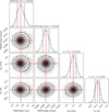 |
Fig. A.1 Distribution of posteriors corresponding to the sinusoidal fit of the ESPRESSO FWHM data. |
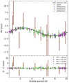 |
Fig. A.2 ESPRESSO and HARPS RVs with the stellar activity signal subtracted and folded in phase with the orbital period of planet GJ7 b. The planet mid-transit time (T0) occurs at half the orbital period. |
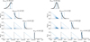 |
Fig. A.3 ExoMDN interior models of GJ7 b displaying the mass fractions of the different layers (left) and thicknesses (right). |
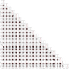 |
Fig. A.4 Distribution of posteriors corresponding to the photometric and spectroscopic solutions for the GJ7 planetary system using TESS SAP fluxes and null eccentricity. |
ESPRESSO radial velocities of GJ7.
ESPRESSO spectral indices.
HARPS radial velocities of GJ7.
Priors adopted for planetary orbit modeling of combined light curves and RV data, along with median values of posterior distributions.
Priors adopted for planetary orbit modeling of combined light curves and RV data, along with median values of posterior distributions, using TESS PDCSAP fluxes.
GJ7 b (TOI-198 b) planetary parameters using PDCSAP fluxes.
All Tables
Priors adopted for planetary orbit modeling of combined light curves and RV data, along with median values of posterior distributions.
Priors adopted for planetary orbit modeling of combined light curves and RV data, along with median values of posterior distributions, using TESS PDCSAP fluxes.
All Figures
|
Fig. 1 TESS TPF of GJ7 (sector 69). The red boxes represent the aperture mask used to extract the photometry. The white cross on top of the largest red circle illustrates the position of GJ7. Other red circles stand for sources of the Gaia DR3 catalog down to 8 magnitudes fainter than our target. This plot was created with the tpfplotter code (Aller et al. 2020). |
| In the text | |
|
Fig. 2 Color-magnitude diagrams displaying the location of GJ7 (TOI-198), the young stellar sequence of Group 29 (Oh et al. 2017; Luhman 2018), the main sequence of M-type stars (Cifuentes et al. 2020), and several confirmed low-metallicity field stars with spectral types M1–M6 from the catalog of Leggett et al. (2000). The dispersion of the main sequence is shown by the gray-shaded area. |
| In the text | |
|
Fig. 3 Photometric spectral energy distribution of GJ7 (circles). The PHOENIX solar-metallicity model (Teff = 3800 K, log g∗ = 5.0 cm s−2) is shown by the gray line normalized to the observed fluxes between 0.8 and 1.6 μm (Husser et al. 2013). Photometric error bars are included, although for most of the wavelengths they have the size of the symbol. The horizontal errors account for the effective width of the filters. At short wavelengths, GJ7 exhibits flux excesses with respect to the photospheric emission indicative of some stellar activity, while at the longest wavelengths, there are no obvious infrared flux excesses. Both axes are on a logarithmic scale. |
| In the text | |
|
Fig. 4 (Left panel): Hertzsprung–Russel diagram of field M-type stars with different metallicities. GJ7 (TOI-198) is depicted by the star symbol. Solar-metallicity stars come from Schweitzer et al. (2019) and low-metallicity stars were collected from Kesseli et al. (2019). Stellar metallicity is color-coded. The 5 Gyr isochrones of the BT-Settl models ([Fe/H] between solar and –2 dex produced by Allard et al. (2013) are depicted by the solid lines. (Right panel): stellar radius versus metallicity. Tracks of constant mass (Allard et al. 2013) are shown by the blue lines. Stellar Teff is color-coded. The stellar radius axis is on a logarithmic scale. |
| In the text | |
|
Fig. 5 Left: ESPRESSO data (blue dots) and their linear trend (green line). Middle and right columns: GLS periodograms of the original data and data corrected for the linear trend. The vertical red line stands for the orbital period of the transiting planet GJ7 b, while the pink band indicates the most likely rotation period of the parent star. The 0.1%, 5%, and 10% FAP levels are plotted with horizontal orange lines. |
| In the text | |
|
Fig. 6 (Top panel) ESPRESSO CCF FWHM (dots) as a function of time, along with the best sinusoidal model (black line) with a rotation period of 47.19 d (linear trend shown by the straight green line). The 1σ uncertainty of the model is depicted by the gray-shaded area. (Bottom panel) Observed minus computed diagram displaying the FWHM residuals. The derived jitter term (thin vertical line) is quadratically added to the nominal errors (thick vertical line). Stellar variability is reasonably well approximated by a sinusoidal function. |
| In the text | |
|
Fig. 7 ESPRESSO spectra around Ca II H and K and Hϵ lines (top), and lithium lines (bottom). Hϵ (in emission) and the lithium doublet wavelengths are marked by vertical red lines. The wavelength is in the air system. No clear lithium feature is observed. |
| In the text | |
|
Fig. 8 Rotation periods of low-mass stars against Teff. GJ7 is depicted by the red star symbol. The 4 Gyr gyrochone defined in Dungee et al. (2022) is shown by the orange line. The members of the M67 cluster used to define the 4 Gyr gyrochrone are displayed by the black dots, while other cluster members are shown by gray dots. |
| In the text | |
|
Fig. 9 TESS SAP fluxes of GJ7 from sectors 2 (top), 29 (middle), and 69 (bottom). Top: modeled covariance function used to flatten the data (black curves) together with the original SAP fluxes (blue points). Bottom: flattened TESS light curves (blue points) and the location of GJ7 b’s transits (black line) registered by TESS. |
| In the text | |
|
Fig. 10 TESS (top) and CHEOPS (bottom) data folded in phase with the planetary orbital period. The white symbols stand for binned data every 51 points (∼ 15 min, TESS) and 19 points (∼19 min, CHEOPS). The black line corresponds to the transit model. Per panel, the bottom, narrower subpanels depict the data residuals. |
| In the text | |
|
Fig. 11 (Top panel) ESPRESSO RV time series (dots), best-fit model (black), and GP model (brown). The gray area stands for the 1σ dispersion of the best solution. (Bottom panel) Observed minus computed residuals. |
| In the text | |
|
Fig. 12 ESPRESSO RVs folded in phase with one stellar rotation period (Keplerian signal removed). |
| In the text | |
|
Fig. 13 Top panel: ESPRESSO RVs, phase-folded with GJ7 b’s orbital period after removing the stellar activity signal, along with the Kep- lerian model (black curve). Bottom panel: observed-minus-computed residuals. The planet’s mid-transit time (T0) corresponds to half an orbital period. |
| In the text | |
|
Fig. 14 Hipparchos-Gaia proper motion acceleration sensitivity to companions of a given mass (in Jupiter masses) as a function of the orbital semimajor axis (in astronomical units) orbiting GJ7. The solid line denotes the combinations of mass and separation explaining the observed proper motion acceleration at the mean epoch of Gaia DR3, based on the analytical formulation of Kervella et al. (2019) and the observed astrometric acceleration for GJ7 reported by Kervella et al. (2022). The shaded light blue region corresponds to the 1σ uncertainty domain. Both axes are plotted on a logarithmic scale. |
| In the text | |
|
Fig. 15 Stellar metallicity [Fe/H] plotted against planetary radius (top) and density (bottom). Over 1000 exoplanets are plotted with their masses (on logarithmic scale) color-coded (darker implies lower planetary mass). These data are taken from the NASA Exoplanet Archive database. GJ7 b is depicted by the red point. The vertical axes are on a logarithmic scale. |
| In the text | |
|
Fig. 16 Top: planetary mass–radius diagram, including all known exoplanets with a radius and a mass constrained to a precision better than 12% (gray, open circles). GJ7 b is depicted by the red circle. Interior models of different compositions (Zeng et al. 2019) are shown by the solid colored lines. Two other planets discussed in the text are labeled. Bottom: planetary insolation plotted as a function of planetary radius for the same planets. The eight planets of the Solar System are shown as a reference. All axes are on a logarithmic scale. |
| In the text | |
|
Fig. 17 Planetary systems containing terrestrial, transiting, low-mass exoplanets with mass Mp ≤ 4 M⊕ and radius constrained to a precision better than 12% are shown relative to the location of the estimated habitable zone (blue-shaded area, Kopparapu et al. 2014). GJ7 and the Solar System are depicted at the top and bottom, respectively. All planetary systems are scaled to GJ7. The size of the black dots is linearly scaled to the radius of the planets (excluding the Solar System). The semimajor axis errors are plotted, and the x-axis is on a logarithmic scale. |
| In the text | |
|
Fig. A.1 Distribution of posteriors corresponding to the sinusoidal fit of the ESPRESSO FWHM data. |
| In the text | |
|
Fig. A.2 ESPRESSO and HARPS RVs with the stellar activity signal subtracted and folded in phase with the orbital period of planet GJ7 b. The planet mid-transit time (T0) occurs at half the orbital period. |
| In the text | |
|
Fig. A.3 ExoMDN interior models of GJ7 b displaying the mass fractions of the different layers (left) and thicknesses (right). |
| In the text | |
|
Fig. A.4 Distribution of posteriors corresponding to the photometric and spectroscopic solutions for the GJ7 planetary system using TESS SAP fluxes and null eccentricity. |
| In the text | |
Current usage metrics show cumulative count of Article Views (full-text article views including HTML views, PDF and ePub downloads, according to the available data) and Abstracts Views on Vision4Press platform.
Data correspond to usage on the plateform after 2015. The current usage metrics is available 48-96 hours after online publication and is updated daily on week days.
Initial download of the metrics may take a while.