| Issue |
A&A
Volume 706, February 2026
|
|
|---|---|---|
| Article Number | A242 | |
| Number of page(s) | 18 | |
| Section | Catalogs and data | |
| DOI | https://doi.org/10.1051/0004-6361/202452293 | |
| Published online | 13 February 2026 | |
Catalog of 13CO clumps from FUGIN in the Milky Way at l = 10°–50°
1
Center for Astronomy and Space Sciences, China Three Gorges University,
Yichang
443000,
China
2
Centre for Astrophysics and Planetary Science, University of Knet,
Canterbury
CT2 7NH,
UK
3
Purple Mountain Observatory, Chinese Academy of Sciences,
Nanjing
210023,
China
4
College of Electrical Engineering and New Energy, China Three Gorges University,
Yichang
443000,
China
★ Corresponding authors: This email address is being protected from spambots. You need JavaScript enabled to view it.
; This email address is being protected from spambots. You need JavaScript enabled to view it.
Received:
18
September
2024
Accepted:
10
December
2025
Abstract
Context. Since stars and star clusters emerge from the gravitational collapse of clumps and cores, studying molecular clumps is fundamental to understanding the processes of star formation. The FOREST Unbiased Galactic Plane Imaging (FUGIN) survey offers insights into the distribution of clumps and physical properties across different environments, aiding in studies of environmental effects, such as the location within the galaxy on star formation.
Aims. This study aims to produce a catalog of clumps from the FUGIN survey to understand the complete mechanism of high-mass star formation in giant molecular clouds (GMCs). We use the catalog to analyze the physical properties of clumps in high-mass star-forming regions, enhancing our understanding of how different environments impact the star-formation process.
Methods. Our process for the detection and verification of 13CO clumps in the FUGIN survey comprised two steps. First, the source extraction code FacetClumps was used to detect as many molecular clump candidates as possible from the FUGIN 13CO data. Second, a trained and validated semi-supervised deep learning model, SS-3D-Clump, was applied to verify these candidates, providing confidence levels for the clumps and filtering out false candidates to enhance the accuracy of the detection results.
Results. The resulting catalog containing 23 150 clumps extracted from the 13CO (J=1–0) data covers the first quadrant (10° ≤ l ≤ 50°, |b| ≤ 1°). By matching with CHIMPS and inheriting the distances of the matched CHIMPS clumps, we found that the sizes of the FUGIN clumps range from 0.1 to 3 pc, demonstrating that the dense structures belong to the clump scale. The catalog achieves an 80% completeness level above 466 K km s−1.
Conclusions. The proposed two-step approach effectively integrates clump detection algorithms with semi-supervised deep learning, achieving an accuracy comparable to manual verification and thereby improving the extraction of clumps from large-scale survey data. The resulting clump catalog enables the analysis of the physical properties of clumps in high-mass star-forming regions, contributing to a better understanding of environmental influences on clump formation and the star formation process.
Key words: molecular data / techniques: image processing / ISM: molecules
© The Authors 2026
 Open Access article, published by EDP Sciences, under the terms of the Creative Commons Attribution License (https://creativecommons.org/licenses/by/4.0), which permits unrestricted use, distribution, and reproduction in any medium, provided the original work is properly cited.
This article is published in open access under the Subscribe to Open model. This email address is being protected from spambots. You need JavaScript enabled to view it. to support open access publication.
1 Introduction
The study of molecular clumps is crucial for advancing theories of star formation since stars and star clusters are formed through the gravitational collapse of these clumps or cores (Krumholz & McKee 2005; Zinnecker & Yorke 2007; Rathborne et al. 2009; Alves de Oliveira et al. 2014; Takekoshi et al. 2019; Rigby et al. 2019; Yoo et al. 2023). Star-forming regions are messy and chaotic environments, with structures existing on many scales (Wurster & Rowan 2023). The entire region is typically referred to as a cloud; dense regions embedded within the cloud are clumps and the very dense regions in the clumps are cores (Alves et al. 2007). The clumps are defined as compact (~1 pc) and dense (~104 H2 cm−3) structures (e.g., Williams et al. 2000; Zhang et al. 2009; Heyer & Dame 2015; Ohashi et al. 2016; Motte et al. 2018; Takekoshi et al. 2019). The mass distribution of clumps provides essential information not only on the mechanisms that influence clump formation, evolution, and destruction (e.g., Rosolowsky 2005; Colombo et al. 2014; Faesi et al. 2016), but also on the crucial factor in constraining theories of star formation (e.g., Alves et al. 2007; Clark et al. 2007; Liu et al. 2022). To determine the role played by environmental effects in the formation and evolution of molecular clumps and how these, in turn, affect star formation, we need to study the properties of clumps in different environments.
Many systematic CO survey projects have focused on the inner and outer Galaxy, such as the Galactic Ring Survey (GRS; Jackson et al. 2006), the CO Heterodyne Inner Milky Way Plane Survey (CHIMPS; Rigby et al. 2016), the Structure, Excitation, and Dynamics of the Inner Galactic Inter-Stellar Medium Survey (SEDIGISM; Schuller et al. 2017), the Milky Way Imaging Scroll Painting Survey (MWISP; Su et al. 2016, 2019), the FOREST Unbiased Galactic Plane Imaging Survey with Nobeyama 45 m telescope (FUGIN; Umemoto et al. 2017), and the Outer Galaxy High-Resolution Survey (OGHReS; Urquhart et al. 2024). These surveys, with their different levels of sensitivity and spatial resolution, can help us to detect the distribution of the molecular component at different scales (Benedettini et al. 2021) from dense clouds and filamentary structures (André et al. 2014) to pre-stellar clumps and young stellar objects.
In the northern inner Galactic plane, GRS (Jackson et al. 2006) covers the region between 18° ≤ l ≤ 55.7° and |b| ≤ 1° in 13CO (J=1–0) at 46″ resolution, providing a benchmark in high-resolution, unbiased spectral imaging. Rathborne et al. (2009) employed the ClumpFind algorithm (Williams et al. 1994) to identify 829 molecular clouds and 6124 clumps, finding that clouds within the 5 kpc ring typically have warmer temperatures, higher column densities, larger areas, and a larger number of clumps. CHIMPS (Rigby et al. 2016) carried out a 13CO and C18O (3–2) survey with the 15-m James Clerk Maxwell Telescope (JCMT), covering a large portion of the GRS survey region (27.8° ≤ l ≤ 46.2° and |b| ≤ 0.5°) with a higher angular resolution of 15″. Based on the CHIMPS 13CO data, Rigby et al. (2019) obtained the first source catalog identified by FellWalker (Berry 2015) and found no significant systematic variations in the physical properties of the sources (e.g., mass, column density, or virial parameter) across the probed range of Galactocentric distances. In the outer Galaxy, OGHReS (Urquhart et al. 2024) is a systematic, high-resolution survey (i.e., θFWHM ≈ 30″) in 12CO (J=2–1) and 13CO (J=2–1), covering the region between 180° ≤ l ≤ 280° and approximately 1° in b. Urquhart et al. (2024) used a subset of the data (250° ≤ l ≤ 280°, −2° ≤ b ≤ 1°) to verify the velocities and distances assigned to the Hi-GAL clumps in this part of the Galaxy (Mège et al. 2021) and to refine their physical properties (Elia et al. 2021), which is crucial for understanding how different environmental conditions affect star formation.
The FOREST Unbiased Galactic Plane Imaging (FUGIN, Umemoto et al. 2017) Survey utilized the Nobeyama 45-meter radio telescope to simultaneously observe the emission spectral lines of three CO isotopologues: 12CO, 13CO, and C18O (J=1–0) in the first quadrant region (10° ≤ l ≤ 50°, |b| ≤ 1°, hereafter QI, shown as the red area in Fig. 1) and the third quadrant region (198° ≤ l ≤ 236°, |b| ≤ 1°, hereafter QIII, shown as the green area in Fig. 1) of the Galaxy. The project achieved 20" angular resolution allows to resolve down to 0.19 pc at 2 kpc distances, which can provide detailed knowledge of the structure and physical properties of the nearest GMCs (Heyer & Dame 2015), ranging from the core scales (~0.1 pc) to cloud scales (10–100 pc). The survey maps areas include the spiral arms (Perseus, Sagittarius, Scutum, and Norma) and star-forming regions (e.g., W31, W33, W39, M16, M17; Beuther et al. 2011; Khan et al. 2022; Kerton et al. 2013; Tremblin et al. 2014; Chen et al. 2021), the bar structure, and the molecular gas ring. It is essential to understand the full mechanism of high-mass star formation in giant molecular clouds (GMCs), particularly by examining the physical properties of cores and clumps in high-mass star-forming regions through large-field surveys (Takekoshi et al. 2019). Comparing these regions, along with the outer Galaxy where the metallicity is much lower (Smartt & Rolleston 1997) and their bar-swept radii, will expand our understanding of the impact of the environment on the star formation process (Eden et al. 2020).
With the progress of Galactic survey projects, various molecular clumps detection algorithms have emerged (Rosolowsky et al. 2008; Berry 2015; Luo et al. 2022; Jiang et al. 2023). The Dendrograms algorithm (Rosolowsky et al. 2008) is well-suited to representing the hierarchical structure of isosurfaces in molecular line data cubes, illustrating variations in topology as contour levels change (Rani et al. 2023). This method has been widely used in conjunction with continuum, atomic hydrogen (HI), and molecular line data (Takekoshi et al. 2019; Nakanishi et al. 2020; Zhang et al. 2021). The FacetClumps algorithm (Jiang et al. 2023) utilizes morphological methods to extract signal regions from raw data and applies the Gaussian facet model (Ji & Haralick 2002) and extremum theory of multivariate functions to locate the centers of clumps. This algorithm enhances the accuracy of region segmentation by dividing signal regions into local areas and subsequently clustering these local regions to the centers of clumps based on connectivity and minimum distance.
A manual confirmation is crucial for the clump candidates obtained using the FacetClumps algorithm noted above to eliminate false positives and ensure the reliability of clump targets in scientific analysis (Rigby et al. 2019). However, large-scale survey projects often yield many clump candidates, making extensive manual verification impractical. Therefore, there is an urgent need for an automated clump verification algorithm to substitute for manual inspection. Luo et al. (2024a) attempted to integrate deep learning into the clump verification process as deep learning has shown outstanding performance in classifying galaxies (Cheng et al. 2020; He et al. 2021), developing the semi-supervised deep clustering algorithm called SS-3D-Clump. The model utilizes a 3D convolutional neural network (3D CNN) to extract features of clumps and classify them using a constrained K-means approach to obtain a pseudo-label. Subsequently, it uses these pseudo labels as supervision to update the weights of SS-3D-Clump. Therefore, SS-3D-Clump can leverage unlabeled samples via a semi-supervised learning to overcome limitations in supervised learning for limited labeled samples and enhance the generalization ability.
This study builds upon the Facet-SS-3D-Clump framework introduced in Luo et al. (2024b), which established a workflow for detecting and verifying 13CO clumps in the MWISP survey. The workflow first uses FacetClumps to identify clump candidates, and then applies SS-3D-Clump for verification. In the present work, we extend the framework by applying it to a broader Galactic region. The paper is organized as follows. Section 2 introduces the observations of FUGIN. Section 3 describes the molecular clump extraction algorithm and the use of SS-3D-Clump to verify clump candidates. In Section 4, we present the catalog containing 23 150 13CO clumps extracted from QI and provide a brief statistical analysis of the spatial distribution of clumps and comparison with CHIMPS clumps. Section 5 presents the conclusion.
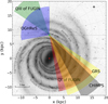 |
Fig. 1 Area of the Galaxy covered by the FUGIN survey. Face-on view of an imaginary Milky Way (credit: R. Hurt, NASA/JPL-Caltech/SSC). The Galactic center (red asterisk) is at (0,0) and the Sun (green filled circle) is at (0, 8.5). |
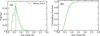 |
Fig. 2 Noise level of the 13CO data. Panel a: histogram of the rms noise levels. Panel b: cumulative distribution of the rms noise levels. |
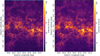 |
Fig. 3 Selected region of the Milky Way (25.25° ≤ b ≤ 26.75°, −1° ≤ l ≤ 1°, and 0 ≤ v ≤ 130 km/s). Left panel displays the integrated map of the S/N data, revealing noticeable horizontal stripes. Right panel shows the result after interpolation, effectively removing the stripes. |
2 Data
2.1 Data introduction
The FUGIN project utilizes the new multi-beam FOREST system, installed on the Nobeyama 45 m telescope to support legacy projects. This four-beam receiver system on the 45 m Telescope is an integrated, dual-polarization, sideband-separating SIS receiver. The four beams are arranged in a 2 × 2 configuration with approximately a 50″ grid, and each beam has angular resolution of around 14″ at 115 GHz. The main beam efficiencies at 86,110, and 115 GHz are 0.56 ± 0.03, 0.45 ± 0.02, and 0.43 ± 0.02, respectively. FUGIN conducts Galactic plane CO observations1 with a 20″ angular resolution for the 12CO and 21″ angular resolution for the 13CO and C18O (J=1–0). The effective velocity resolution is 1.3 km s−1 at 115 GHz. The root mean square (rms) distribution is shown in Fig. 2, and the median noise level for the 13CO spectra is 0.62 K.
2.2 Preprocessing of 13CO data
We first selected a local region in the first quadrant of the Milky Way: 25.25° ≤ l ≤ 26.75°, −1° ≤ b ≤ 1°, and 0 km s−1 ≤ v ≤ 130 km s−1, as shown in Fig. 3. The left panel of Fig. 3 shows the integrated map of the region’s signal-to-noise ratio (S/N) data in velocity. The map reveals noticeable horizontal stripes in the data. The right panel of Fig. 3 displays the result after interpolating the striped data. It can be seen from the map that the stripes have been reduced, although some faint residual patterns remain. As an example, we use a section of data from one velocity channel (see the left panel of Fig. 4), which clearly shows horizontal stripes. The specific processing steps are as follows:
The first step is to apply a threshold of 3×rms to the image to generate a binary map. A horizontal projection (i.e., integration along the Galactic longitude direction) is then performed on this binary map, resulting in the blue curve (shown in Fig. 5).
In the second step, a moving average filter with a fixed window size (9 pixels) is applied to the blue curve to obtain the orange curve. This filter effectively suppresses high-frequency noise while preserving the overall trend of the data by computing the arithmetic mean within the window. Stripe regions are identified based on the peak-valley structures of the two curves; specifically, areas where the orange curve significantly exceeds the blue curve are considered candidate stripe regions, as these correspond to weakened intensity features. These regions are highlighted as blue-shaded areas in Fig. 5 and the final detected stripe regions are mapped back onto the original data, as shown in Fig. 6.
The third step involves using the data surrounding the detected stripe regions to interpolate and fill in the stripes using the cubic spline interpolation algorithm (Ooyama 2002; Karpfinger 2022). The cubic spline method fits a set of piecewise cubic polynomials between data points, ensuring the continuity of the first and second derivatives across segment boundaries, which results in a smooth and natural-looking reconstruction. The final processed result is shown in the right panel of Fig. 4. After processing the striped data in FUGIN, the map of 13CO integrated with velocity from -9 to 128 km s−1 for the FUGIN (Umemoto et al. 2017) in QI is shown in Appendix D (Fig. D.1). It was drawn using the Cube Analysis and Rendering Tool2 for Astronomy (Carta, Angus Comrie et al. 2021).
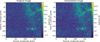 |
Fig. 4 Example illustrating the interpolation of stripes in the data. Left panel shows the original data with stripes. Right panel shows the data after the interpolation processing. |
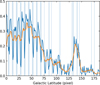 |
Fig. 5 Horizontal projection curve of the original image after binarization is shown, where the blue curve represents the original projection curve, and the orange is the result of applying a moving average to the original curve. The blue shaded areas indicate the regions of stripes in the image. Note: the vertical axis in the figure has no actual physical significance; it only represents the ratio of pixels exceeding 3×rms to the total number of pixels in the horizontal direction. |
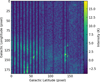 |
Fig. 6 Stripe regions are overlaid onto the original data and for easier observation, the X and Y axes of the image have been swapped. |
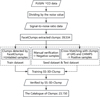 |
Fig. 7 Workflow for obtaining a clumps catalog. |
3 Generation of a 13CO clump catalog from FUGIN
Stars are formed within interstellar molecular clouds, primarily composed of molecular gases. The hierarchical structure of the molecular phase of the ISM can be broadly categorized into three structures: clouds, clumps, and cores (Alves et al. 2007; Wurster & Rowan 2023). Clumps refer to regions of increased density within more giant clouds. They can also be identified as continuous areas in the l–b–v space (where l, b, and v represent Galactic longitude, latitude, and velocity, respectively). Cores are highly dense regions within clumps. They result from the fragmentation of larger clumps and may eventually collapse to form individual stars or star clusters (Blitz & Williams 1999; Bergin & Tafalla 2007). This study defines the compact structure traced by 13CO as a “clump”.
The 13CO clumps detection and verification process of FUGIN is illustrated in Fig. 7, which comprises two major steps. First, FacetClumps (Jiang et al. 2023) was used to detect and obtain molecular clump candidates from FUGIN 13CO data. As mentioned by Medina et al. (2019), it is doubtful that a false detection would randomly appear in the same position in other independent surveys. Therefore, we assumed that any candidate with a counterpart in a published catalog was real. We labeled the candidates matched with clumps in GRS (Rathborne et al. 2009) and CHIMPS (Rigby et al. 2019) as real sources, which then served as the seed set in the training process of SS-3D-Clump (Luo et al. 2024a). Negative samples were obtained through manual verification (see the right panel of Fig. C.1 in Appendix C). Second, the trained and stabilized SS-3D-Clump is applied to verify the candidates, obtaining confidence levels (i.e., predicted probabilities between 0 and 1) for the molecular clumps. After the process above, we obtained a catalog of molecular clumps, including their positions, peak, integrated intensity, and confidence levels associated with the clumps.
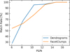 |
Fig. 8 Matching ratios of FacetClumps and Dendrograms in the three regions data as a function of the PS/N of the clumps. The orange curve represents the fraction of FacetClumps that have a corresponding Dendrogram clump, while the blue curve represents the fraction of Dendrogram clumps that have a corresponding FacetClump clump. |
3.1 Clumps extraction
We observed a noticeable and uneven noise level in FUGIN data due to the non-uniform sensitivity of the survey, which could lead to overlooking clumps in regions with noise below the average level and, conversely, misidentifying false clumps as real ones in high-noise areas. Following the approach of Rigby et al. (2016), who conducted source extraction on the CHIMPS survey on S/N data cubes, these were obtained by dividing the observational data by the corresponding noise. We also applied FacetClumps to the S/N data to detect molecular clumps and generate masks. We selected three local regions along the Galactic longitude in QI, spanning different density ranges. Using these three representative regions, we compared and analyzed the detection results of the FacetClumps and Dendrograms algorithms as a benchmark against existing mature algorithms.
Figure 8 shows the matching ratios between the FacetClumps and Dendrogram extractions in the three regions as a function of the peak S/N (PS/N) of the clumps. The matching ratio is defined as the fraction of clumps in one catalog that have at least one spatially overlapping counterpart in the other. Specifically, the orange curve represents the fraction of FacetClumps that have corresponding Dendrogram clumps, while the blue curve represents the fraction of Dendrogram clumps that have corresponding FacetClump clumps. As shown in Fig. 8, when the PS/N of the clumps rises above 12, the matching rate exceeds 90% across the data of three regions with different densities, and the detection results of the two algorithms become consistent. Detailed experiments and results are presented in Appendix A.
FacetClumps3 (Jiang et al. 2023) employs the Gaussian facet model to fit the local surfaces and determine clump centers through the extremum determination theorem of multivariate functions. Based on the identified clump centers, FacetClumps clusters the regions near the centers by considering connectivity and minimum distance, thereby obtaining molecular clumps. Since the detection data is based on S/N data, the background rms equals unity. The parameter Threshold is the minimum intensity used to truncate the signal, defined by its relationship to the background rms and set to 4. Another parameter, SRecursionLBV, is used to determine the minimum area of a region in the spatial direction (SRecursionLB) and the minimum length of a region in the velocity channels (SRecursionV) when a recursion terminates. The parameter breaks down the volume parameter used in other algorithms, such as Dendrograms (Rosolowsky et al. 2008) and FellWalker (Berry 2015), into the minimum area in the spatial direction and the minimum extent in the velocity direction. It helps further eliminate false detections caused by elongated noise, as such noise can still meet the minimum volume parameter criteria. SRecursionLB is set to 25 square pixels, corresponding to an angular size of approximately 0.5 square arcminutes, and SRecursionV is set to 5 pixels, corresponding to a velocity of 3.25 km s−1. The other parameters of FacetClumps are set to the default values of the algorithm.
3.2 The seed dataset and test dataset
There are roughly three methods to obtain high-confidence molecular clumps: (1) using different algorithms to detect the same dataset. Thus, if multiple algorithms detect a target, the probability that this target is real will be high; (2) using different data for validation. Thus, if a molecular clump detected in the 13CO data is also detected in the C18O data, the probability that the corresponding 13CO clump is real will also be high; and (3) by matching with other published catalogs. Thus, if a molecular clump can match with an existing source catalog, the probability that it is real will also be high, as reported in Medina et al. (2019).
This paper adopts the same strategy as in Medina et al. (2019), based on establishing matches with published catalogs to obtain a reliable sample of molecular clumps, which would then be considered a robust sample. We used the topcat4 tool from the Starlink package to match the clump candidates with the clumps in GRS (Rathborne et al. 2009) and CHIMPS (Rigby et al. 2019). The matching was performed based on the centroid positions of the clumps, requiring deviations of less than 1′ in Galactic longitude and latitude and less than 2 km s−1 in velocity. In the overlapping region between FUGIN and GRS, which contains 16 292 FUGIN clumps and 5868 GRS clumps, we have 3242 GRS clumps that were successfully matched with at least one FUGIN counterpart. Between FUGIN and CHIMPS, which have 7171 and 4473 clumps in the overlapping region, respectively, there were 2476 CHIMPS clumps found to have FUGIN counterparts. The strict matching criteria were adopted to ensure a high-confidence sample of molecular clumps for subsequent analysis. Figure 9 shows the results of two matched molecular clumps in CHIMPS and FUGIN. The first column shows two clumps from CHIMPS, while the second column shows the corresponding matched clumps from FUGIN.
To obtain sample of false detections (i.e., incorrectly identified molecular clumps), we first need to identify the clumps that can be confidently regarded as real based on the following criteria: 1. the molecular clumps must first exhibit enhanced intensity in the local region, showing significant intensity peaks on the integrated maps in three directions (Galactic longitude, Galactic latitude, and velocity); and 2. in the spectral line information of the velocity direction, the clump’s average spectrum and peak spectrum must display a Gaussian profile.
Clumps that satisfy these two conditions are considered real by manual verification and the remaining ones are regarded as false detections. For example, Fig. C.1 in Appendix C shows two examples of clumps verified as “true” and as “false.”
We compiled a test dataset containing 2000 true detections and 1000 false detections. The true detections are the ones that were matched with clumps in the GRS and CHIMPS. The false detections were identified through visual inspection and confirmed not to correspond to any real clump structures. Additionally, we separated some samples from the test dataset to form a seed dataset, which includes 300 real and 300 false detections. We note that the test dataset does not participate in the model training. The seed sample set was used to ensure proper model convergence. The primary data used for model training consists of many unlabeled sample data. The model principles and the role of the data will be explained in detail in the next section.
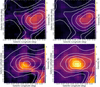 |
Fig. 9 Examples of two matched clumps in CHIMPS and FUGIN are shown. The first column shows two clumps from CHIMPS, while the second column shows the corresponding matched clumps from FUGIN. The contours in the figure are drawn on the intensity map of the FUGIN clumps and overlaid onto the map of the CHIMPS clumps. |
3.3 Verification by SS-3D-Clump
SS-3D-Clump5 is a semi-supervised learning method designed to verify molecular clumps by Luo et al. (2024a). It consists of three main modules: a feature extraction module utilizing a 3D CNN, a pseudo-label acquisition module employing an unsupervised clustering algorithm and a fully connected network (FCN) for label prediction. The input to SS-3D-Clump is a 3D cube with the size set to 30 px × 30 px × 30 px, centered on the clump candidate. Each cube is extracted from the 13CO spectral line data. During training, the model is fed shuffled mini-batches sampled from the full training dataset in each iteration, and the entire dataset is reshuffled at the start of every epoch to enhance generalization. The SS-3D-Clump outputs a confidence value between 0 and 1, indicating the likelihood that a given candidate is a real clump.
From an intuitive perspective, if two clumps share similar physical characteristics, they are expected to remain close in the learned feature space after being processed by a feature extraction model. This means their separation (i.e., feature distance) will be small and their similarity high. The SS-3D-Clump framework is built on this principle. Initially, the trainable parameters of the feature extraction and classification networks in the SS-3D-Clump are randomly initialized and tasked with learning a feature mapping that transforms clump candidates into a high-dimensional space where structurally similar clumps are grouped together. To generate training labels without requiring manual annotation, we adopted an unsupervised strategy using the K-means clustering algorithm (Han et al. 2012; Ay et al. 2023), whose initial cluster centers were determined on the basis of the high-confidence seed samples. In each training iteration, K-means is applied to the extracted features to assign each sample to one of two clusters, interpreted as pseudo-labels. It should be noted that the two clusters obtained by the K-means algorithm are not intended to represent the physical subclasses of molecular clumps. Instead, they provide a fundamental distinction between “normal” and “potentially anomalous” samples, serving as pseudo-labels for the subsequent semi-supervised classification. The number of clusters was empirically determined based on the stability and convergence behavior of the SS-3D-Clump, as increasing the cluster number often resulted in fragmented or unstable groupings without improving the detection accuracy, while simply using two clusters ensured a more stable convergence and consistent classification results.
These pseudo-labels are then used to construct a classification loss function, enabling supervised-style training via backpropagation. During the early stages of training, the model’s feature extraction capability is still under development and the resulting pseudo-labels are often unstable. As training progresses, however, the model gradually learns to represent similar clumps with increasingly similar features, leading to more consistent and accurate cluster assignments. To further guide the convergence process, we introduced a small number of high-confidence “seed” samples with fixed labels to constrain the K-means algorithm (Basu et al. 2002) and accelerate model learning.
Some statistical metrics (Cunha et al. 2024), such as precision (P), recall (R), F1 score (F1), and accuracy (Acc), were used to quantify the performance of SS-3D-Clump in the test dataset. The calculation formulas of R, P, F1, and Acc are as follows:
![Mathematical equation: $\[R=\frac{T P}{T P+F N},\]$](/articles/aa/full_html/2026/02/aa52293-24/aa52293-24-eq1.png) (1)
(1)
![Mathematical equation: $\[P=\frac{T P}{T P+F P},\]$](/articles/aa/full_html/2026/02/aa52293-24/aa52293-24-eq2.png) (2)
(2)
![Mathematical equation: $\[F_1=2 \times \frac{P \times R}{P+R},\]$](/articles/aa/full_html/2026/02/aa52293-24/aa52293-24-eq3.png) (3)
(3)
![Mathematical equation: $\[A c c=\frac{T P+T N}{T P+T N+F P+F N},\]$](/articles/aa/full_html/2026/02/aa52293-24/aa52293-24-eq4.png) (4)
(4)
where TP (true-positive) is the number of sources predicted to be true and actual is true, FP (false-positive) is the number of sources predicted to be true and actual is false, TN (true-negative) is the number of sources predicted to be false and actual is false, and FN (false-negative) is the number of sources predicted to be false and actual is true.
Acc measures the proportion of correct predictions across all classes relative to the total number of predictions. P indicates the proportion of correct predictions for a specific class compared to the total number of predictions for that class, focusing on the quality of positive predictions. R represents the proportion of correct predictions for a specific class relative to that class’s total number of positive cases. Combining P and R yields informative metrics like F1, the harmonic mean of P and R.
Figure 10 shows those evaluation indications of SS-3D-Clump in verifying the samples in the test dataset after each iteration during the training process. As shown from the top two subplots in Fig. 10, the model exhibits high accuracy, but low recall during the first ten training epochs, as the insufficiently trained model tends to classify most samples as negative. As training iterations increase, the recall rate rises sharply while the accuracy decreases slightly. After 30 training iterations, all metrics stabilize, with precision and recall approaching 90% and 95%. It is noteworthy that this level of accuracy is achieved using only seed samples of 300 real and 300 false-positive clumps, indicating that the SS-3D-Clump can find similarities and differences among data through training, enabling it to recognize molecular clumps effectively, even in large-scale training projects with massive sample sizes.
We measured the information shared between two different cluster assignments A and B, each corresponding to a different training epoch, using normalized mutual rnformation (NMI, Caron et al. 2018). In this context, an epoch refers to a complete pass through the training dataset during model optimization. As the SS-3D-Clump model trains, it generates different cluster assignments at each epoch. By computing NMI(A; B) between successive epochs (e.g., A at epoch t − 1 and B at epoch t), we can monitor the evolution of the predicted assignments and assess the convergence and stability of the clustering process. The NMI is calculated as
![Mathematical equation: $\[N M I(A; B)=\frac{M I(A; B)}{\sqrt{H(A) H(B)}},\]$](/articles/aa/full_html/2026/02/aa52293-24/aa52293-24-eq5.png) (5)
(5)
where MI denotes the mutual information and H the entropy. Overall, NMI can be applied to any assignment from the clusters or the true labels. The value of NMI typically falls between 0 and 1, where 1 indicates complete similarity between two clustering results, and 0 signifies no resemblance. Therefore, the NMI curves can be utilized to observe how the performance of SS-3D-Clump changes with increasing number of training epochs, facilitating the optimization of the model training process. The bottom panel in Fig. 10 illustrates the NMI curve changing with the epochs during the training process of SS-3D-Clump, it can be observed that the NMI increases to ~0.98 at the 30th epoch and remains stable thereafter. This indicates that SS-3D-Clump is experiencing fewer reassignments and the clusters are stabilizing.
Utilizing the stabilized SS-3D-Clump model, we verified the candidates detected by FacetClumps by computing their confidence values, which represent the predicted probability that a given candidate is a real molecular clump. As shown in Fig. 11, the receiver operating characteristic (ROC) curve (Rojas et al. 2022; Demianenko et al. 2023) yields an optimal classification threshold of 0.712, with an area under the curve (AUC) of 0.938, indicating that the model effectively distinguishes between clump and non-clump samples. To simplify interpretation while preserving high-confidence selections, we adopted a slightly rounded threshold of 0.7. Candidates with confidence values below this threshold were rejected.
As a result, SS-3D-Clump excluded 16 384 of the 39 534 clump candidates, leaving a final catalog of 23 150 molecular clumps. Figure 12 shows the histograms of clump PS/N values. The green histogram represents the PS/N distribution of clumps obtained by FacetClumps, while the red histogram shows the distribution of PS/N values for clumps excluded by SS-3D-Clump. The blue curve indicates the proportion of clumps retained by SS-3D-Clump as a function of the PS/N. Figure 12 shows that the PS/N of the clumps verified as false by SS-3D-Clump is primarily below 10. Combining this with the results from the algorithm benchmark tests, where detection results of various algorithms converge and show high accuracy when the PS/N exceeds 12 (see Fig. 8), it is evident that SS-3D-Clump is able to effectively exclude false-positive detections. This experiment demonstrates that combining detection algorithms with deep learning-based verification techniques can allow us to achieve results that match the reliability of combining the results from detections made with multiple algorithms. In practical scenarios, this approach enables the detection algorithms to identify as many candidates as possible for high recall rates, while SS-3D-Clump enhances the accuracy of the resulting clump catalog.
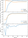 |
Fig. 10 Accuracy and recall metrics of SS-3D-Clump on the test dataset as the epoch of the training process changes. Evolution of cluster reassignments (NMI) in each clustering iteration of SS-3D-Clump. |
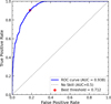 |
Fig. 11 Receiver operating characteristic (ROC) curve of the SS-3D-Clump model. The optimal threshold of 0.712 yields an area under the curve (AUC) of 0.938. |
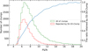 |
Fig. 12 Histogram illustrating the PS/N distribution of clumps molecular clump candidates obtained by Facet-SS-3D-Clump. The green bars represent the distribution of clumps obtained by FacetClumps, while the red bars represent these rejected by SS-3D-Clump. The blue curve indicates the proportion of clumps retained by SS-3D-Clump as a function of the PS/N. |
4 Result
Using the two-step method for detecting and verifying clumps, there were 23 150 13CO clumps extracted from QI of FUGIN, covering the first quadrant region (10° ≤ l ≤ 50°, |b| ≤ 1°). The names, units, symbols, and detailed descriptions of the columns in the molecular clump catalog are provided in Table 1. Following the definition of Berry (2015), we define the intensity-weighted second-moment sizes (or RMS sizes) along each axis as
![Mathematical equation: $\[S_l=\sqrt{\frac{\sum_i I_i\left(l_i-\bar{l}\right)^2}{\sum_i I_i}}, \quad S_b=\sqrt{\frac{\sum_i I_i\left(b_i-\bar{b}\right)^2}{\sum_i I_i}},]$](/articles/aa/full_html/2026/02/aa52293-24/aa52293-24-eq6.png) (6)
(6)
where Ii is the intensity of the voxel, i, while ![Mathematical equation: $\[\bar{l}\]$](/articles/aa/full_html/2026/02/aa52293-24/aa52293-24-eq7.png) and
and ![Mathematical equation: $\[\bar{b}\]$](/articles/aa/full_html/2026/02/aa52293-24/aa52293-24-eq8.png) are the intensity-weighted centroids defined as
are the intensity-weighted centroids defined as
![Mathematical equation: $\[\bar{l}=\frac{\sum_i I_i l_i}{\sum_i I_i}, \quad \bar{b}=\frac{\sum_i I_i b_i}{\sum_i I_i}.\]$](/articles/aa/full_html/2026/02/aa52293-24/aa52293-24-eq9.png) (7)
(7)
For sources with purely Gaussian intensity profiles, this RMS size corresponds to the standard deviation of the Gaussian along the corresponding axis, namely,
![Mathematical equation: $\[I(l) \propto ~\exp \left[-\frac{(l-\bar{l})^2}{2 \sigma_l^2}\right], \quad I(b) \propto ~\exp \left[-\frac{(b-\bar{b})^2}{2 \sigma_b^2}\right],\]$](/articles/aa/full_html/2026/02/aa52293-24/aa52293-24-eq10.png) (8)
(8)
the intensity-weighted RMS sizes reduce exactly to the Gaussian standard deviations. Thus, for purely Gaussian clumps, the RMS sizes directly correspond to the standard deviations of the profiles along each axis.
FUGIN 13CO (J=1–0) clump catalog.
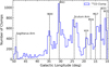 |
Fig. 13 Distribution of 13CO clumps along the Galactic longitude. The dashed line represents the star-forming region or spiral arm in the QI. |
4.1 Galactic distribution
Due to the sparse distribution of molecular gas in the QIII, only a few molecular clumps (167) are detected, we consider exploring the analysis of the outer Galaxy as a separate case study. This would allow for a more detailed investigation by matching the outer Galaxy data with OGHReS (Urquhart et al. 2024) observations to examine star formation metrics. In this study, the spatial analysis is limited to the QI. The longitude distribution of 13CO clumps is shown in Fig. 13, where the dashed lines mark the locations of known star-forming regions or spiral arms within QI. Similarly to Beuther et al. (2012); Molinari et al. (2016), we identify in Fig. 13 prominent features that can be associated with major star-forming complexes or with the tangents of spiral arms. Specifically, the overdensities near l ~ 23° and l ~ 49° correspond to the Scutum and Sagittarius arms, respectively, where the line of sight intersects dense molecular gas and active star-forming regions. This figure reveals clustering of 13CO clumps near the longitude of the star-forming region or spiral arm.
The latitude distribution of clumps in the QI is shown in Fig. 14. In the left panel of this figure, we show the mean and standard deviation of the distribution of clumps along latitude for different longitude intervals. The filled blue circles represent the mean latitude of the clumps within each longitude interval, with error bars indicating the size of their standard deviation. The blue histogram shown in the right panel of Fig. 14 shows the distribution of molecular clumps obtained by Facet-SS-3D-Clump and the blue dashed line indicating the mean value of latitude. The histogram peaks at slightly negative values with a mean value of b = −0.136°. As Molinari et al. (2016) pointed out, this may be attributed to an incorrect assumption about the vertical position of the Sun in the Milky Way. The latitude distribution of molecular clumps exhibits an asymmetrical pattern.
In Fig. 15, we show the centers of clumps in the longitude-velocity (l − v) plane and the relevant sprial arm features (Reid et al. 2014). Dashed lines indicate the near side of the arms and solid lines represent the respective far side. In addition to the correlation between the spiral arms, we also find significant numbers of sources coincident with the Aquila Rift (34°, 11 km s−1) and Aquila Spur (37°, 80 km s−1). The good correlation with these spiral features provides confidence that the detected sources are genuine and that the number of false detections is low.
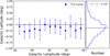 |
Fig. 14 Latitude distribution of clumps in the QI. The left part illustrates the mean and standard deviation of clump distribution along latitude for various longitude intervals. Blue circular points denote the mean latitude within each interval, with error bars representing the standard deviation. The right part shows a latitude distribution of QI clumps, with the blue dashed line indicating the mean latitude. |
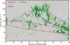 |
Fig. 15 Centers of clumps in the l–v plane are illustrated. The lines indicate the spiral arm loci of Norma, Scutum, and Sagittarius, as well as the smaller Aquila spur and Aquila Rift as estimated by Reid et al. (2014). The near and far sides of the arms are dotted and solid lines, respectively. |
4.2 Comparison with CHIMPS
CHIMPS is a high resolution 13CO and C18O (J=3–2) survey of ~20 square degrees of the first quadrant (θ = 15″ and 27.8° ≤ l ≤ 46.2° and |b| ≤ 0.5°; Rigby et al. 2016). Rigby et al. (2019) obtained the first source catalog consisting of 4999 clumps identified by FellWalker Berry (2015) in the 13CO emission maps. Comparing the CHIMPS sources with the sources extracted from FUGINS provides a benchmark for our method. The selection of CHIMPS over GRS was motivated by two principal considerations. First, the angular resolution of CHIMPS (15″) closely matches that of FUGIN (20″), while GRS exhibits a significantly coarser resolution (46″). This resolution compatibility ensures more reliable one-to-one (or one-to-many) matching between the catalogs, effectively minimizing systematic biases arising from spatial scale mismatches. Second, while both surveys observe the 13CO line, they probe different rotational transitions (J=3–2 for CHIMPS versus J=1–0 for FUGIN). This configuration not only facilitates future investigations of excitation conditions across transitions but also provides unique opportunities to study the physical properties and evolutionary stages of star-forming structures through multi-transition analysis. Consequently, CHIMPS offers both methodological robustness and scientific added value for verifying and expanding upon our results.
Using the matching criteria described in Section 3.3, we obtained 2476 CHIMPS sources with a FUGIN counterpart. The FUGIN catalog for the overlapping CHIMPS region contains 7171 clumps and 5934 FUGIN clumps have corresponding CHIMPS clumps. The observed asymmetry in matched clumps (5934 FUGIN clumps associated with 2476 CHIMPS clumps) reflects a complex interplay between detection thresholds and molecular line properties. The higher S/N threshold used in FUGIN (≥4) preferentially isolates prominent emission peaks, especially within the more diffuse 13CO (J=1–0) line, which is sensitive to cold and extended molecular gas. This tends to fragment extended structures into multiple smaller clumps. In contrast, CHIMPS employs a lower S/N threshold (≥2), allowing for more extended J=3–2 emission to be grouped into single clumps, often merging adjacent substructures into larger ones. Moreover, the J=3–2 line traces warmer and denser regions, typically found in the compact centers of star-forming molecular clouds, which may appear as continuous, larger-scale structures. As a result, many small FUGIN clumps can fall within the extent of a single CHIMPS clump, naturally leading to a one-to-many matching relationship.
It should be noted that the process of cross-matching clumps identified in different transitions is subject to intrinsic physical limitations. The 13CO (J=1–0) transition used in FUGIN primarily traces colder and more diffuse molecular gas, while the 13CO (J=3–2) line observed in CHIMPS is excited under warmer and denser conditions. As a result, some clumps that are clearly detected in the J=1–0 emission might fall below the excitation threshold of the J=3–2 line and vice versa. These differences in excitation temperature, optical depth, and critical density naturally lead to incomplete one-to-one correspondence between the catalogs.
Figure 16 shows the relative deviations in Galactic longitude and latitude between FUGIN clumps that have matched counterparts in CHIMPS. The relative deviation (ε) is defined as
![Mathematical equation: $\[\varepsilon=\frac{d_{c e n}}{d_{s i z e}},\]$](/articles/aa/full_html/2026/02/aa52293-24/aa52293-24-eq12.png) (9)
(9)
where dcen is the distance between the centroids of the matched clumps and dsize is the sum of the size of the matched clumps in Galactic longitude or latitude. The blue and orange bars in Fig. 16 represent the relative deviations of the matched clumps in Galactic longitude and latitude, respectively. The figure shows that most matched clumps (~72%) have a relative deviation of less than 25%.
Figure 17 shows the flux distribution of FUGIN clumps within the CHIMPS region and the flux distribution of clumps matched with CHIMPS. The blue bars represent the flux distribution of FUGIN clumps in the CHIMPS region, while the orange bars represent the flux distribution of clumps with CHIMPS counterparts. As can be seen from the figure, the flux of clumps without a CHIMPS counterpart is primarily concentrated on the left side of the distribution, indicating that these clumps tend to be smaller or less intense.
Based on the matching results, we adopted the distances (d) from the clumps in CHIMPS and calculated the equivalent radii for the clumps in FUGIN. The equivalent radius was defined consistently with the value given in CHIMPS (Rigby et al. 2019), calculated as ![Mathematical equation: $\[R_{\sigma}=d \sqrt{S_{l} S_{b}}\]$](/articles/aa/full_html/2026/02/aa52293-24/aa52293-24-eq13.png) , where d is the distance in parsecs, and Sl and Sb are angular sizes in radians. Here, Sl and Sb represent the intensity-weighted root-mean-square (rms) deviations of voxels from the clump centroid along the Galactic longitude and latitude axes, respectively. Figure 18 shows the equivalent radii of the matched clumps in FUGIN and CHIMPS. The horizontal axis represents the equivalent radii of the clumps in FUGIN, while the vertical axis represents the equivalent radii of the corresponding matched clumps in CHIMPS. As seen in Fig. 18, most clumps in FUGIN have equivalent radii within the range of 0.1–1 pc, with a few exceeding 1 pc but all within 3 pc. It indicates that the dense structures detected in the FUGIN 13CO data primarily correspond to clump-scale structures.
, where d is the distance in parsecs, and Sl and Sb are angular sizes in radians. Here, Sl and Sb represent the intensity-weighted root-mean-square (rms) deviations of voxels from the clump centroid along the Galactic longitude and latitude axes, respectively. Figure 18 shows the equivalent radii of the matched clumps in FUGIN and CHIMPS. The horizontal axis represents the equivalent radii of the clumps in FUGIN, while the vertical axis represents the equivalent radii of the corresponding matched clumps in CHIMPS. As seen in Fig. 18, most clumps in FUGIN have equivalent radii within the range of 0.1–1 pc, with a few exceeding 1 pc but all within 3 pc. It indicates that the dense structures detected in the FUGIN 13CO data primarily correspond to clump-scale structures.
A comparison between the equivalent radii of the matched FUGIN and CHIMPS clumps reveals a power-law relation expressed as ![Mathematical equation: $\[R_{\text {CHIMPS}}=1.17 \times R_{\text {FUGIN}}^{0.91}\]$](/articles/aa/full_html/2026/02/aa52293-24/aa52293-24-eq14.png) , as shown in Fig. 18. The Pearson correlation coefficient between the two sets of radii is 0.60, indicating a moderate positive correlation. This suggests that the sizes of CHIMPS clumps are generally comparable to, but slightly larger than, those in FUGIN, and they tend to scale consistently on average. It should be noted that the two extractions were performed on different 13CO transitions J=3–2 for CHIMPS and J=1–0 for FUGIN. A likely explanation lies in the different detection thresholds: the FellWalker algorithm used for CHIMPS allows voxels with S/N ≥ 2 to be included in a clump, while in FUGIN, a stricter threshold of S/N ≥ 4 is applied. As a result, CHIMPS clumps tend to include more low-intensity surrounding voxels, leading to slightly larger segmented regions.
, as shown in Fig. 18. The Pearson correlation coefficient between the two sets of radii is 0.60, indicating a moderate positive correlation. This suggests that the sizes of CHIMPS clumps are generally comparable to, but slightly larger than, those in FUGIN, and they tend to scale consistently on average. It should be noted that the two extractions were performed on different 13CO transitions J=3–2 for CHIMPS and J=1–0 for FUGIN. A likely explanation lies in the different detection thresholds: the FellWalker algorithm used for CHIMPS allows voxels with S/N ≥ 2 to be included in a clump, while in FUGIN, a stricter threshold of S/N ≥ 4 is applied. As a result, CHIMPS clumps tend to include more low-intensity surrounding voxels, leading to slightly larger segmented regions.
Figure 19 shows the distribution of velocity dispersion for the matched FUGIN-CHIMPS clumps. The velocity dispersion of FUGIN clumps is mainly concentrated between 0.6 and 1.5 km s−1, with the distribution peaking at 0.8 km s−1. Notably, the FUGIN distribution lacks clumps with velocity dispersions below 0.6 km s−1, which are present in the CHIMPS sample. This discrepancy arises from the extraction criteria applied in the FUGIN clump identification process, which require a minimum velocity extent of five consecutive channels (corresponding to 3.25 km s−1) for a clump to be considered. Since the velocity dispersion Δv is defined as the intensity-weighted rms deviation from the centroid in velocity axis, this threshold effectively excludes clumps with narrow linewidths. Assuming a Gaussian line profile with a full width of five channels (approximately 6σ), the minimum Δv would be around 0.504 km s−1, which is consistent with the lower bound observed in the FUGIN distribution. As a result, some low-Δv clumps present in CHIMPS were not recovered in FUGIN due to this velocity constraint.
We also compared the peak intensities of molecular clumps matched between FUGIN and CHIMPS. As shown in Fig. 20, the peak intensities of most FUGIN clumps are stronger than those of CHIMPS clumps, which may be because the excitation conditions for the J = 3 → 2 transition are higher than those for the J = 1 → 0 transition, resulting in lower radiation temperatures. Another noteworthy point is that the scatter plot of the matched FUGIN and CHIMPS clumps exhibits a power-law distribution. The fitted power-law index is 1.82, indicating that as the intensity of the molecular clumps increases, the intensity of the J = 3 → 2 clumps increases more rapidly. The Pearson correlation coefficient between the logarithmic peak intensities of the two datasets is 0.43, indicating a weak to moderate linear correlation in log-log space. The considerable scatter visible in Fig. 20 suggests that this relationship is not tightly constrained, likely reflecting intrinsic physical differences between the tracers: the J = 3 → 2 transition traces warmer and denser gas with higher critical densities, whereas the J = 1 → 0 line is more sensitive to extended, lower-density molecular envelopes.
The FUGIN 13CO (J=1–0) clump catalog presented in this study complements existing large-scale molecular clump catalogs such as GRS (13CO J=1–0) and CHIMPS (13CO J=3–2). With its high-resolution coverage and consistent clump identification criteria applied across the first Galactic quadrant, this catalog provides a valuable resource for investigating environmental variations in molecular clump structure and star formation efficiency in the inner Milky Way. Moreover, the dataset can be directly compared with GRS and CHIMPS to probe excitation conditions, evolutionary stages, and line-ratio diagnostics, thereby facilitating comprehensive multi-transition analyses of Galactic molecular gas. A detailed excitation analysis for the FUGIN and CHIMPS-matched molecular clumps is presented in a separate study.
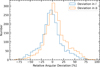 |
Fig. 16 Relative angular deviations of matched clumps in Galactic longitude and latitude. Blue bars represent the deviations in Galactic longitude, while orange bars represent the deviations in Galactic latitude. |
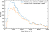 |
Fig. 17 Flux distribution of all FUGIN clumps within the CHIMPS region (blue bars) and the flux distribution of FUGIN clumps matched with CHIMPS (orange bars). |
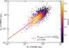 |
Fig. 18 Comparison of the radii of FUGIN clumps matched to CHIMPS clumps. The distances of the FUGIN clumps are set to match these of their corresponding CHIMPS clumps. The red line represents the fitted relationship, with a correlation coefficient of 0.6. The color bar on the right indicates the local density of data points, normalized to unity, meaning that the region with the highest concentration of points has a normalized density of 1. |
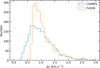 |
Fig. 19 Comparison of Δv of the matched FUGIN-CHIMPS clumps. |
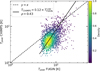 |
Fig. 20 Comparison of Tpeak of the matched FUGIN-CHIMPS clumps. |
5 Conclusion
We utilized Facet-SS-3D-Clump for the detection and verification of molecular clumps in the 13CO data within FUGIN, covering the longitude range 10° ≤ l ≤ 50° and a latitude strip of |b| ≤ 1°. We obtained a catalog containing 23 150 13CO clumps. We summarize our conclusions below.
First, the Facet-SS-3D-Clump workflow leverages a clump detection algorithm combined with semi-supervised deep learning to effectively search for and verify dense structures in large-scale survey projects, achieving accuracy comparable to manual verification and making comprehensive molecular clump surveys feasible. Second, these molecular clumps align well with the star-forming regions and spiral arms, exhibiting a mean Galactic latitude significantly below the midplane, with b = −0.136°. Third, this catalog provides data support for analyzing the physical properties of clumps in high-mass star-forming regions, enhancing our understanding of the role of environmental effects in the formation and evolution of clumps and how different environments impact the star formation process. Finally, the flux completeness limits were presented: the catalog is 80% complete above 466 K km s−1.
Data availability
Full table 1 is available at the CDS via https://cdsarc.cds.unistra.fr/viz-bin/cat/J/A+A/706/A242.
Acknowledgements
This publication makes use of data from FUGIN, the FOREST Unbiased Galactic plane Imaging survey with the Nobeyama 45-m telescope, a legacy project of the Nobeyama 45-m radio telescope. We are grateful to all the members of the FUGIN working group. This work was supported by the National Natural Science Foundation of China (U2031202, 11903083, 11873093, and 12203029). Software: CARTA (Angus Comrie et al. 2021), Astropy (Astropy Collaboration 2013, 2018; Astropy Collaboration 2022), TensorFlow (Abadi et al. 2015), Scikit-Learn (Pedregosa et al. 2011).
References
- Abadi, M., Agarwal, A., Barham, P., et al. 2015, TensorFlow: Large-Scale Machine Learning on Heterogeneous Systems, software available from https://tensorflow.org [Google Scholar]
- Alves, J., Lombardi, M., & Lada, C. J. 2007, A&A, 462, L17 [NASA ADS] [CrossRef] [EDP Sciences] [Google Scholar]
- Alves de Oliveira, C., Schneider, N., Merín, B., et al. 2014, A&A, 568, A98 [NASA ADS] [CrossRef] [EDP Sciences] [Google Scholar]
- André, P., Di Francesco, J., Ward-Thompson, D., et al. 2014, in Protostars and Planets VI, eds. H. Beuther, R. S. Klessen, C. P. Dullemond, & T. Henning, 27 [Google Scholar]
- Angus Comrie, Kuo-Song Wang, Shou-Chieh Hsu, et al. 2021, CARTA: The Cube Analysis and Rendering Tool for Astronomy [Google Scholar]
- Astropy Collaboration (Robitaille, T. P., et al.) 2013, A&A, 558, A33 [NASA ADS] [CrossRef] [EDP Sciences] [Google Scholar]
- Astropy Collaboration (Price-Whelan, A. M., et al.) 2018, AJ, 156, 123 [Google Scholar]
- Astropy Collaboration (Price-Whelan, A. M., et al.) 2022, ApJ, 935, 167 [NASA ADS] [CrossRef] [Google Scholar]
- Ay, M., Özbakır, L., Kulluk, S., et al. 2023, Expert Syst. Appl., 211, 118656 [Google Scholar]
- Basu, S., Banerjee, A., & Mooney, R. J. 2002, in Machine Learning, Proceedings of the Nineteenth International Conference (ICML 2002), University of New South Wales, Sydney, Australia, July 8–12, 2002 [Google Scholar]
- Benedettini, M., Traficante, A., Olmi, L., et al. 2021, A&A, 654, A144 [NASA ADS] [CrossRef] [EDP Sciences] [Google Scholar]
- Bergin, E. A., & Tafalla, M. 2007, ARA&A, 45, 339 [Google Scholar]
- Berry, D. S. 2015, Astron. Comput., 10, 22 [Google Scholar]
- Beuther, H., Linz, H., Henning, T., et al. 2011, A&A, 531, A26 [NASA ADS] [CrossRef] [EDP Sciences] [Google Scholar]
- Beuther, H., Tackenberg, J., Linz, H., et al. 2012, ApJ, 747, 43 [Google Scholar]
- Blitz, L., & Williams, J. P. 1999, The Origin of Stars and Planetary Systems, eds. C. J. Lada & N. D. Kylafis, 540, 3 [Google Scholar]
- Caron, M., Bojanowski, P., Joulin, A., & Douze, M. 2018, in Proceedings of the European Conference on Computer Vision (ECCV) [Google Scholar]
- Chen, Z., Sun, W., Chini, R., et al. 2021, ApJ, 922, 90 [NASA ADS] [CrossRef] [Google Scholar]
- Cheng, T.-Y., Conselice, C. J., Aragón-Salamanca, A., et al. 2020, MNRAS, 493, 4209 [Google Scholar]
- Clark, P. C., Klessen, R. S., & Bonnell, I. A. 2007, MNRAS, 379, 57 [NASA ADS] [CrossRef] [Google Scholar]
- Colombo, D., Hughes, A., Schinnerer, E., et al. 2014, ApJ, 784, 3 [NASA ADS] [CrossRef] [Google Scholar]
- Cunha, P. A. C., Humphrey, A., Brinchmann, J., et al. 2024, A&A, 687, A269 [NASA ADS] [CrossRef] [EDP Sciences] [Google Scholar]
- Demianenko, M., Malanchev, K., Samorodova, E., et al. 2023, A&A, 677, A16 [NASA ADS] [CrossRef] [EDP Sciences] [Google Scholar]
- Eden, D. J., Moore, T. J. T., Currie, M. J., et al. 2020, MNRAS, 498, 5936 [NASA ADS] [CrossRef] [Google Scholar]
- Elia, D., Merello, M., Molinari, S., et al. 2021, MNRAS, 504, 2742 [NASA ADS] [CrossRef] [Google Scholar]
- Faesi, C. M., Lada, C. J., & Forbrich, J. 2016, ApJ, 821, 125 [NASA ADS] [CrossRef] [Google Scholar]
- Han, J., Kamber, M., & Pei, J. 2012, in Data Mining, third edn., eds. J. Han, M. Kamber, & J. Pei, The Morgan Kaufmann Series in Data Management Systems (Boston: Morgan Kaufmann), 497 [Google Scholar]
- He, Z., Qiu, B., Luo, A. L., et al. 2021, MNRAS, 508, 2039 [NASA ADS] [CrossRef] [Google Scholar]
- Heyer, M., & Dame, T. 2015, ARA&A, 53, 583 [NASA ADS] [CrossRef] [Google Scholar]
- Jackson, J. M., Rathborne, J. M., Shah, R. Y., et al. 2006, ApJS, 163, 145 [NASA ADS] [CrossRef] [Google Scholar]
- Ji, Q., & Haralick, R. M. 2002, Pattern Recognit., 35, 689 [Google Scholar]
- Jiang, Y., Chen, Z., Zheng, S., et al. 2023, ApJS, 267, 32 [NASA ADS] [CrossRef] [Google Scholar]
- Karpfinger, C. 2022, Polynomial and Spline Interpolation (Berlin, Heidelberg: Springer Berlin Heidelberg), 311 [Google Scholar]
- Kerton, C. R., Arvidsson, K., & Alexander, M. J. 2013, AJ, 145, 78 [Google Scholar]
- Khan, S., Pandian, J. D., Lal, D. V., et al. 2022, A&A, 664, A140 [NASA ADS] [CrossRef] [EDP Sciences] [Google Scholar]
- Krumholz, M. R., & McKee, C. F. 2005, ApJ, 630, 250 [Google Scholar]
- Liu, L., Bureau, M., Li, G.-X., et al. 2022, MNRAS, 517, 632 [NASA ADS] [CrossRef] [Google Scholar]
- Luo, X., Zheng, S., Huang, Y., et al. 2022, Res. Astron. Astrophys., 22, 015003 [CrossRef] [Google Scholar]
- Luo, X., Zheng, S., Jiang, Z., et al. 2024a, A&A, 683, A104 [NASA ADS] [CrossRef] [EDP Sciences] [Google Scholar]
- Luo, X., Zheng, S., Jiang, Z., et al. 2024b, Res. Astron. Astrophys., 24, 055018 [Google Scholar]
- Medina, S. N. X., Urquhart, J. S., Dzib, S. A., et al. 2019, A&A, 627, A175 [NASA ADS] [CrossRef] [EDP Sciences] [Google Scholar]
- Mège, P., Russeil, D., Zavagno, A., et al. 2021, A&A, 646, A74 [NASA ADS] [CrossRef] [EDP Sciences] [Google Scholar]
- Molinari, S., Schisano, E., Elia, D., et al. 2016, A&A, 591, A149 [NASA ADS] [CrossRef] [EDP Sciences] [Google Scholar]
- Motte, F., Bontemps, S., & Louvet, F. 2018, ARA&A, 56, 41 [NASA ADS] [CrossRef] [Google Scholar]
- Nakanishi, H., Fujita, S., Tachihara, K., et al. 2020, PASJ, 72, 43 [CrossRef] [Google Scholar]
- Ohashi, S., Sanhueza, P., Chen, H.-R. V., et al. 2016, ApJ, 833, 209 [NASA ADS] [CrossRef] [Google Scholar]
- Ooyama, K. V. 2002, Monthly Weather Rev., 130, 2392 [Google Scholar]
- Pedregosa, F., Varoquaux, G., Gramfort, A., et al. 2011, J. Mach. Learn. Res., 12, 2825 [Google Scholar]
- Rani, R., Moore, T. J. T., Eden, D. J., et al. 2023, MNRAS, 523, 1832 [NASA ADS] [CrossRef] [Google Scholar]
- Rathborne, J. M., Johnson, A. M., Jackson, J. M., Shah, R. Y., & Simon, R. 2009, ApJS, 182, 131 [NASA ADS] [CrossRef] [Google Scholar]
- Reid, M. J., Menten, K. M., Brunthaler, A., et al. 2014, ApJ, 783, 130 [Google Scholar]
- Rigby, A. J., Moore, T. J. T., Plume, R., et al. 2016, MNRAS, 456, 2885 [NASA ADS] [CrossRef] [Google Scholar]
- Rigby, A. J., Moore, T. J. T., Eden, D. J., et al. 2019, A&A, 632, A58 [NASA ADS] [CrossRef] [EDP Sciences] [Google Scholar]
- Rojas, K., Savary, E., Clément, B., et al. 2022, A&A, 668, A73 [NASA ADS] [CrossRef] [EDP Sciences] [Google Scholar]
- Rosolowsky, E. 2005, PASP, 117, 1403 [NASA ADS] [CrossRef] [Google Scholar]
- Rosolowsky, E. W., Pineda, J. E., Kauffmann, J., & Goodman, A. A. 2008, ApJ, 679, 1338 [Google Scholar]
- Schuller, F., Csengeri, T., Urquhart, J. S., et al. 2017, A&A, 601, A124 [NASA ADS] [CrossRef] [EDP Sciences] [Google Scholar]
- Smartt, S. J., & Rolleston, W. R. J. 1997, ApJ, 481, L47 [Google Scholar]
- Su, Y., Sun, Y., Li, C., et al. 2016, ApJ, 828, 59 [Google Scholar]
- Su, Y., Yang, J., Zhang, S., et al. 2019, ApJS, 240, 9 [Google Scholar]
- Takekoshi, T., Fujita, S., Nishimura, A., et al. 2019, ApJ, 883, 156 [NASA ADS] [CrossRef] [Google Scholar]
- Tremblin, P., Schneider, N., Minier, V., et al. 2014, A&A, 564, A106 [NASA ADS] [CrossRef] [EDP Sciences] [Google Scholar]
- Umemoto, T., Minamidani, T., Kuno, N., et al. 2017, PASJ, 69, 78 [Google Scholar]
- Urquhart, J. S., König, C., Colombo, D., et al. 2024, MNRAS, 528, 4746 [Google Scholar]
- Williams, J. P., de Geus, E. J., & Blitz, L. 1994, ApJ, 428, 693 [Google Scholar]
- Williams, J. P., Blitz, L., & McKee, C. F. 2000, in Protostars and Planets IV, eds. V. Mannings, A. P. Boss, & S. S. Russell, 97 [Google Scholar]
- Wurster, J., & Rowan, C. 2023, MNRAS, 523, 3025 [NASA ADS] [CrossRef] [Google Scholar]
- Yoo, H., Lee, C. W., Chung, E. J., et al. 2023, ApJ, 957, 94 [Google Scholar]
- Zhang, Q., Wang, Y., Pillai, T., & Rathborne, J. 2009, ApJ, 696, 268 [Google Scholar]
- Zhang, S., Zavagno, A., López-Sepulcre, A., et al. 2021, A&A, 646, A25 [NASA ADS] [CrossRef] [EDP Sciences] [Google Scholar]
- Zinnecker, H., & Yorke, H. W. 2007, ARA&A, 45, 481 [Google Scholar]
Appendix A Comparison with Dendrograms
As a benchmark against existing mature algorithms, three local regions along the Galactic longitude in QI, spanning different density ranges, were selected to compare and analyze the detection results of the FacetClumps and Dendrograms algorithms. Three selected regions are centered at Galactic longitudes 12°, 28°, and 44°, each covering an area of one square degree. The first region spans a Galactic longitude range of 11.5 to 12.5°, a Galactic latitude range of -0.87 to 0.13°, and a velocity range of -10 to 80 km s−1 (hereafter called Cell_12). The second region: 27.65° ≤ l ≤ 28.65°, −0.6° ≤ b ≤ 0.4°, and 12 km s−1 ≤ v ≤ 112 km s−1 (hereafter called Cell_28). The third region: 43.65° ≤ l ≤ 44.65°, −0.46° ≤ b ≤ 0.54°, and 0 km s−1 ≤ v ≤ 100 km s−1 (hereafter called Cell_44). Figure A.1 shows the intensity information for Cell_12, Cell_28, and Cell_44 in the top, middle, and bottom panels, respectively. For each cell, the first, second, and third columns display the integrated intensity maps projected along the velocity, Galactic latitude and Galactic longitude axes, respectively.
Dendrograms (Rosolowsky et al. 2008) algorithm implemented in astrodendro6 is an abstraction of the changing topology of the isosurfaces as a function of contour level. It uses a tree diagram to describe hierarchical structures over various scales in a 2D or 3D datacube (Zhang et al. 2021). The results return two types of structures: leaves, which have no substructure, and branches, which can split into multiple branches or leaves. The algorithm has two main parameters: Tmin and ΔT. The parameter Tmin represents the minimum data value to be considered, and is set to 4. The parameter ΔT defines the required contrast for a leaf to be identified as an independent clump and a value of ΔT = 1 is used, implying that a clump must have a peak intensity of at least 5. The other parameter is the minimum volume parameter (Vmin = 125), which ensures that the retained clumps have a minimum pixel volume. The above parameter settings are all configured for S/N data and are consistent with the parameters used in FacetClumps (see detail in Section 3.1). FacetClumps detected 463, 317, and 128 clumps in Cell_12, Cell_28, and Cell_44, respectively, while Dendrograms detected 318, 198, and 88 clumps.
We matched the detection results of FacetClumps and Dendrograms, taking into account the region and intensity information of the clumps. The specific matching criterion was considered a match when the sum of intensities in the overlapping region accounted for 25% of the sum of intensities within the clump regions detected by each algorithm. We did not use the intersection-over-union (IoU) as the matching standard because different algorithms may produce varying segmentations of the same data and detect different numbers of clumps. For example, in the first rows of Fig. A.3, Dendrograms detected one clump, while FacetClumps detected two. If IoU were used, one of the clumps detected by FacetClumps (marked by a yellow line) would have a low IoU, even though both algorithms detected this clump. Table A.1 provides detailed information on the detection and matching results of the two algorithms across the three regions. We defined a matching ratio, the ratio of matches between the two algorithms to each algorithm’s total number of detections. This ratio represents the matching ratio for the corresponding algorithm. By comparing the detection and matching results across different regions, it can be observed that as the data density decreases, the detection results of the two algorithms become more consistent.
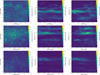 |
Fig. A.1 The information for Cell_12, Cell_28, and Cell_44 are shown in the top, middle, and bottom panels, respectively. The first, second, and third columns show the integrated maps for these regions in Galactic longitude, Galactic latitude, and velocity directions. |
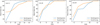 |
Fig. A.2 Matching ratios of FacetClumps and Dendrograms for Cell_12, Cell_28, and Cell_44 in the left, middle, and right subplots, respectively, as a function of the PS/N of the clumps. |
The detailed information on the detection and matching results of the two algorithms across the three regions.
Table A.1 presents the overall matching results of the two algorithms across the three regions. Clumps with higher intensities are more likely to be detected by both algorithms. To investigate this effect quantitatively, we grouped the clumps by their PS/N values and calculated the corresponding detection and matching statistics. As shown in Fig. A.2, the left, middle, and right subplots display the matching rates of FacetClumps and Dendrograms for Cell_12, Cell_28, and Cell_44 as a function of the PS/N of the clumps, respectively. As shown in Fig. A.2, when the PS/N of the clumps rises above 10, the matching rate exceeds 90% across the data of three regions with different densities, and the detection results of the two algorithms become consistent. When the matching rate of both algorithms reaches 100%, it indicates that the detection results of the two algorithms are fully consistent in terms of coverage, with every clump detected by one algorithm having at least one corresponding match in the other, and no clumps left unmatched.
As shown in Fig. A.2, in the Cell_12 data, when the PS/N exceeds 15, the matching rates of both algorithms reach 100%, indicating that all clumps above this threshold are matched between the two algorithms. In the Cell_28 and Cell_44 data, this occurs at approximately PS/N > 11. We then counted the clumps in these three regions that met these PS/N conditions. FacetClumps detected 65 clumps across these regions, while Dendrograms detected 45. The experimental results suggest that FacetClumps detects slightly more clumps than Dendrograms. One possible reason, as illustrated in the first row of Fig. A.3, is that the results detected by Dendrograms are more extended, potentially including multiple local peaks. At the same time, FacetClumps is more compact, enabling the detection of some of these local peaks.
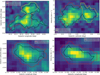 |
Fig. A.3 Examples of detection and matching results between FacetClumps and Dendrograms: The first row shows the matching result of two clumps detected by FacetClumps and one detected by Dendrograms. The left subplot displays the velocity-integrated map of the subregion containing the detected clumps, with the black line marking the boundary of the clump detected by Dendrograms and the red and yellow lines marking the boundaries of the two clumps detected by FacetClumps. The right subplot is similar, except the integration is along the Galactic longitude. The second row shows the matching result of one clump detected by each algorithm, with the rest of the details consistent with the first row. |
Appendix B Completeness Test
The completeness limit refers to the total flux or mass above which an algorithm can detect a clump at a certain level. To quantify the completeness of the extracted clumps, we conducted extensive synthesis data experiments by injecting simulated clumps into the 13CO (J = 1–0) data in FUGIN. The simulated clumps had randomly assigned axis sizes and peak intensities within specified ranges: the peak intensity ranged from 1.5 to 15 K, the velocity-axis size ranged from 1 to 4 pixels, and the spatial size (in Galactic longitude and latitude) ranged from 2 to 6 pixels. These simulated clumps were randomly injected into the FUGIN data, with the constraint being to avoid overlap with another clump.
The recovery fraction as a function of the integrated flux density in different latitude intervals in QI is shown in Fig. B.1. From Fig. B.1, the completeness curves decrease sharply when the flux of clumps is lower than 500 K km s−1 in different latitude intervals. When the completeness reaches 80%, the total flux of clumps is approximately 466 K km s−1 in the QI (black line).
In Fig. B.2, the dashed line represents the completeness limit as a function of Galactic latitude. Meanwhile, the histogram shows the distribution of missed simulated clumps in each Galactic latitude bin. From Fig. B.2, it can be observed that within the Galactic longitude range of 10° to 36°, the flux corresponding to 80% completeness remains around 500 K km s−1, significantly higher than the 200 K km s−1 in the 36° to 50°. It implies that in the 10° to 36°, only larger and brighter molecular clumps can be detected. It can be explained by the fact that numerous star-forming regions within the 10° to 36° lead to a higher data volume and density of molecular clumps, as depicted in Fig. 13.
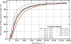 |
Fig. B.1 Completeness fractions as a function of flux density in different Galactic latitude intervals within QI, corresponding to molecular clumps in the extracted catalog with statistically the same sizes. The Galactic latitude range from 10° to 50° is divided into 5-degree bins. The bold black curve represents the completeness curve throughout the entire QI region. |
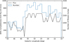 |
Fig. B.2 Eighty percent completeness limits in flux density for a population of clumps with the same distribution of sizes as the one extracted by FacetClumps as a function of Galactic longitude. |
Appendix C Manual Verification
A small portion of the clumps was manually verified according to the criteria described in Section 3.2 to obtain accurate labels for clump samples. To illustrate the differences between true and false clumps, Fig. C.1 presents two representative examples. The top set corresponds to a true molecular clump, while the bottom set shows a false detection. For each case, the first row displays integrated maps along the velocity, Galactic latitude and Galactic longitude axes. The second row shows the same projections, but only retaining emission within the clump boundary to highlight its morphology. The third row shows the clump’s average spectrum, with the red vertical line indicating the centroid velocity and the shaded region representing the velocity range.
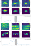 |
Fig. C.1 Example of a true (top) and false (bottom) molecular clump. Each example includes integrated maps (first row), masked maps retaining the clump region (second row), and the clump’s average spectrum (third row), with red lines marking centroid velocity, and the shaded area indicating the velocity range. |
Appendix D The maps of the FUGIN 13CO data
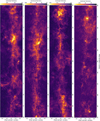 |
Fig. D.1 Integrated intensity maps of the 13CO data over the velocity range -9 to 128 km s−1. A S/N threshold of 2 was applied before integration, and pixels below this threshold were masked. |
All Tables
The detailed information on the detection and matching results of the two algorithms across the three regions.
All Figures
|
Fig. 1 Area of the Galaxy covered by the FUGIN survey. Face-on view of an imaginary Milky Way (credit: R. Hurt, NASA/JPL-Caltech/SSC). The Galactic center (red asterisk) is at (0,0) and the Sun (green filled circle) is at (0, 8.5). |
| In the text | |
|
Fig. 2 Noise level of the 13CO data. Panel a: histogram of the rms noise levels. Panel b: cumulative distribution of the rms noise levels. |
| In the text | |
|
Fig. 3 Selected region of the Milky Way (25.25° ≤ b ≤ 26.75°, −1° ≤ l ≤ 1°, and 0 ≤ v ≤ 130 km/s). Left panel displays the integrated map of the S/N data, revealing noticeable horizontal stripes. Right panel shows the result after interpolation, effectively removing the stripes. |
| In the text | |
|
Fig. 4 Example illustrating the interpolation of stripes in the data. Left panel shows the original data with stripes. Right panel shows the data after the interpolation processing. |
| In the text | |
|
Fig. 5 Horizontal projection curve of the original image after binarization is shown, where the blue curve represents the original projection curve, and the orange is the result of applying a moving average to the original curve. The blue shaded areas indicate the regions of stripes in the image. Note: the vertical axis in the figure has no actual physical significance; it only represents the ratio of pixels exceeding 3×rms to the total number of pixels in the horizontal direction. |
| In the text | |
|
Fig. 6 Stripe regions are overlaid onto the original data and for easier observation, the X and Y axes of the image have been swapped. |
| In the text | |
|
Fig. 7 Workflow for obtaining a clumps catalog. |
| In the text | |
|
Fig. 8 Matching ratios of FacetClumps and Dendrograms in the three regions data as a function of the PS/N of the clumps. The orange curve represents the fraction of FacetClumps that have a corresponding Dendrogram clump, while the blue curve represents the fraction of Dendrogram clumps that have a corresponding FacetClump clump. |
| In the text | |
|
Fig. 9 Examples of two matched clumps in CHIMPS and FUGIN are shown. The first column shows two clumps from CHIMPS, while the second column shows the corresponding matched clumps from FUGIN. The contours in the figure are drawn on the intensity map of the FUGIN clumps and overlaid onto the map of the CHIMPS clumps. |
| In the text | |
|
Fig. 10 Accuracy and recall metrics of SS-3D-Clump on the test dataset as the epoch of the training process changes. Evolution of cluster reassignments (NMI) in each clustering iteration of SS-3D-Clump. |
| In the text | |
|
Fig. 11 Receiver operating characteristic (ROC) curve of the SS-3D-Clump model. The optimal threshold of 0.712 yields an area under the curve (AUC) of 0.938. |
| In the text | |
|
Fig. 12 Histogram illustrating the PS/N distribution of clumps molecular clump candidates obtained by Facet-SS-3D-Clump. The green bars represent the distribution of clumps obtained by FacetClumps, while the red bars represent these rejected by SS-3D-Clump. The blue curve indicates the proportion of clumps retained by SS-3D-Clump as a function of the PS/N. |
| In the text | |
|
Fig. 13 Distribution of 13CO clumps along the Galactic longitude. The dashed line represents the star-forming region or spiral arm in the QI. |
| In the text | |
|
Fig. 14 Latitude distribution of clumps in the QI. The left part illustrates the mean and standard deviation of clump distribution along latitude for various longitude intervals. Blue circular points denote the mean latitude within each interval, with error bars representing the standard deviation. The right part shows a latitude distribution of QI clumps, with the blue dashed line indicating the mean latitude. |
| In the text | |
|
Fig. 15 Centers of clumps in the l–v plane are illustrated. The lines indicate the spiral arm loci of Norma, Scutum, and Sagittarius, as well as the smaller Aquila spur and Aquila Rift as estimated by Reid et al. (2014). The near and far sides of the arms are dotted and solid lines, respectively. |
| In the text | |
|
Fig. 16 Relative angular deviations of matched clumps in Galactic longitude and latitude. Blue bars represent the deviations in Galactic longitude, while orange bars represent the deviations in Galactic latitude. |
| In the text | |
|
Fig. 17 Flux distribution of all FUGIN clumps within the CHIMPS region (blue bars) and the flux distribution of FUGIN clumps matched with CHIMPS (orange bars). |
| In the text | |
|
Fig. 18 Comparison of the radii of FUGIN clumps matched to CHIMPS clumps. The distances of the FUGIN clumps are set to match these of their corresponding CHIMPS clumps. The red line represents the fitted relationship, with a correlation coefficient of 0.6. The color bar on the right indicates the local density of data points, normalized to unity, meaning that the region with the highest concentration of points has a normalized density of 1. |
| In the text | |
|
Fig. 19 Comparison of Δv of the matched FUGIN-CHIMPS clumps. |
| In the text | |
|
Fig. 20 Comparison of Tpeak of the matched FUGIN-CHIMPS clumps. |
| In the text | |
|
Fig. A.1 The information for Cell_12, Cell_28, and Cell_44 are shown in the top, middle, and bottom panels, respectively. The first, second, and third columns show the integrated maps for these regions in Galactic longitude, Galactic latitude, and velocity directions. |
| In the text | |
|
Fig. A.2 Matching ratios of FacetClumps and Dendrograms for Cell_12, Cell_28, and Cell_44 in the left, middle, and right subplots, respectively, as a function of the PS/N of the clumps. |
| In the text | |
|
Fig. A.3 Examples of detection and matching results between FacetClumps and Dendrograms: The first row shows the matching result of two clumps detected by FacetClumps and one detected by Dendrograms. The left subplot displays the velocity-integrated map of the subregion containing the detected clumps, with the black line marking the boundary of the clump detected by Dendrograms and the red and yellow lines marking the boundaries of the two clumps detected by FacetClumps. The right subplot is similar, except the integration is along the Galactic longitude. The second row shows the matching result of one clump detected by each algorithm, with the rest of the details consistent with the first row. |
| In the text | |
|
Fig. B.1 Completeness fractions as a function of flux density in different Galactic latitude intervals within QI, corresponding to molecular clumps in the extracted catalog with statistically the same sizes. The Galactic latitude range from 10° to 50° is divided into 5-degree bins. The bold black curve represents the completeness curve throughout the entire QI region. |
| In the text | |
|
Fig. B.2 Eighty percent completeness limits in flux density for a population of clumps with the same distribution of sizes as the one extracted by FacetClumps as a function of Galactic longitude. |
| In the text | |
|
Fig. C.1 Example of a true (top) and false (bottom) molecular clump. Each example includes integrated maps (first row), masked maps retaining the clump region (second row), and the clump’s average spectrum (third row), with red lines marking centroid velocity, and the shaded area indicating the velocity range. |
| In the text | |
|
Fig. D.1 Integrated intensity maps of the 13CO data over the velocity range -9 to 128 km s−1. A S/N threshold of 2 was applied before integration, and pixels below this threshold were masked. |
| In the text | |
Current usage metrics show cumulative count of Article Views (full-text article views including HTML views, PDF and ePub downloads, according to the available data) and Abstracts Views on Vision4Press platform.
Data correspond to usage on the plateform after 2015. The current usage metrics is available 48-96 hours after online publication and is updated daily on week days.
Initial download of the metrics may take a while.