| Issue |
A&A
Volume 706, February 2026
|
|
|---|---|---|
| Article Number | A236 | |
| Number of page(s) | 15 | |
| Section | Extragalactic astronomy | |
| DOI | https://doi.org/10.1051/0004-6361/202452831 | |
| Published online | 13 February 2026 | |
A deep ALMA Band 3 survey of HDFS/MUSE3D
Survey description and initial results
1
Joint ALMA Observatory Alonso de Córdova 3107 Vitacura 763-0355 Santiago, Chile
2
European Southern Observatory, Alonso de Córdova 3107 Vitacura Casilla 19001 Santiago de Chile, Chile
3
Instituto de Estudios Astrofísicos, Facultad de Ingeniería y 455 Ciencias, Universidad Diego Portales Av. Ejército Libertador 441 Santiago Chile
4
European Southern Observatory Karl-Schwarzschild-Str. 2 85748 Garching Germany
5
National Radio Astronomy Observatory 520 Edgemont Road Charlottesville VA, 22903 USA
★ Corresponding author: This email address is being protected from spambots. You need JavaScript enabled to view it.
Received:
31
October
2024
Accepted:
19
November
2025
Abstract
Context. After more than 10 years of ALMA operations, the community interest in conducting deep extra-galactic millimetre surveys resulted in varying strategic compromises between areal size and map depth to survey the sky. The current bias leans towards a galaxy population found in the field or towards rich starbursty proto-cluster groups, which are both tendentiously surveyed at coarse spatial resolutions.
Aims. We describe a survey that addresses these biases. A deep 3 mm survey was conducted with ALMA at long baselines in a 1 × 1 arcmin2 region in the Hubble Deep Field South (HDFS) that was also covered by the Multi Unit Spectroscopic Explorer (MUSE) in order to assess resolved molecular gas properties in galaxies in group environments at z > 1.
Methods. ALMA observations comprising a four-pointing mosaic with a single band 3 (3 mm) spectral tuning were conducted to cover CO transitions from different groups identified by MUSE. This work consists of a total effective on-source time of 61 hours in configurations with baselines up to 15 km.
Results. The final dataset yields an angular resolution of 0.15″–0.2″ (depending on the imaging weights) and maximum recoverable scales of 1″–2″. The final continuum map reaches an unprecedented sensitivity of RMS ∼ 2 μJy/beam, which allowed us to detect three sources at 3 mm (only one of which with multi-wavelength counterparts from the rest-frame UV to radio). Moreover, we detected six line emitters associated with CO J = 2 − 1 at zspec = 1.284, one of which was not previously detected by MUSE, and none of which was detected in 3 mm continuum. The inter-stellar medium gas masses range from ∼2 × 10⁹ to ∼9 × 10¹⁰ M⊙ (adopting αCO = 4 M⊙/(K.km/s.pc2), including helium). This galaxy group is quite diverse overall, and no two galaxies are alike. Some are clearly offset physically with respect to Hubble imaging that traces the rest-frame ultra-violet emission. We also derived cosmic molecular gas mass densities using this sample as a reference for group environments and found that their densities are similar to that of the galaxy population found in field environments.
Key words: ISM: kinematics and dynamics / ISM: molecules / galaxies: general / galaxies: groups: general / galaxies: ISM
© The Authors 2026
 Open Access article, published by EDP Sciences, under the terms of the Creative Commons Attribution License (https://creativecommons.org/licenses/by/4.0), which permits unrestricted use, distribution, and reproduction in any medium, provided the original work is properly cited.
This article is published in open access under the Subscribe to Open model. This email address is being protected from spambots. You need JavaScript enabled to view it. to support open access publication.
1. Introduction
The advent of the Atacama Large (sub-)Millimetre Array (ALMA; Brown et al. 2004; Cortes et al. 2025) enabled the community to conduct multiple deep extra-galactic surveys at unprecedented angular resolution and sensitivity with which the inter-stellar medium (ISM) gas in galaxies in the early Universe was studied (Hatsukade et al. 2016; Walter et al. 2016; Dunlop et al. 2017; Franco et al. 2018; Hatsukade et al. 2018; Hill et al. 2024). Different groups gave priority to either survey depth or size, but ALMA brought another capability to the table that revolutionised our knowledge of the molecular gas content until cosmic noon and beyond (z ≳ 2). By planning deep fields to be covered at multiple frequency setups (the so-called spectral scans) in different ALMA bands, the community was able to blindly detect the faint dust and molecular gas emissions from galaxy populations while simultaneously determining their distance (e.g., Walter et al. 2016). This resulted in exquisite galaxy samples with which the carbon monoxide (CO) luminosity functions, and by extension, molecular gas (H2) mass functions, were determined (Decarli et al. 2016, 2019; Riechers et al. 2019; Lenkić et al. 2020). Although this was expected based on relations such as the Schmidt-Kennicutt law (Schmidt 1959; Kennicutt 1998), the community finally saw, for the first time, that the cosmological evolution of H2 mass density (ρH2) is indeed closely followed by the density evolution of the star formation rate (Decarli et al. 2016, 2019; Magnelli et al. 2020; Walter et al. 2020), which both peak around 10 Gyr ago (z ∼ 2; the so-called cosmic noon).
For practical reasons, all these surveys are detection experiments in nature. They were conducted with compact configurations in order to avoid resolving out extended emission. As a result, the spatial resolutions of these surveys are planned to be of arcsecond scales. Moreover, because they are blind surveys within known extra-galactic fields, the underlying bias of these samples was towards field galaxy populations. It is now well known, however, that the group environment plays a major role in the evolution of galaxies (Fujita 2004; Vulcani et al. 2015, 2017; Bianconi et al. 2018). The surveys conducted by ALMA that targeted galaxy groups are clearly biased towards rich proto-clusters (e.g., Miller et al. 2018; Oteo et al. 2018), where extremely starbursting galaxies lie close to each other (≪1 Mpc). On the other hand, ALMA surveys towards peaks in the cosmic infrared background (e.g., Kneissl et al. 2019; Hill et al. 2025) also showed groups of main-sequence galaxies with extreme star-forming rates (see also Miller et al. 2018; Oteo et al. 2018). In order to change this trend, we conducted a 1 × 1 arcmin2 deep single-tuning survey at sub-arcsecond scales with ALMA to target two galaxy groups identified at zspec = 1.284 and 4.699 in a deep survey (27 h on source; Bacon et al. 2015, B15) conducted with the Multi Unit Spectroscopic Explorer (MUSE; Bacon et al. 2010) on the European Southern Observatory Very Large Telescope (European Southern Observatory 1998).
The structure of this paper is as follows: Section 2 describes the field selection, the choice of spatial and spectral coverage, the observational strategy, and the resulting survey properties. The initial results are presented in Section 3, with a characterisation of the survey depth, the achieved angular and maximum recovered scales, and a first characterisation of the line and continuum emitters in the field. We present our concluding remarks in Section 4. Throughout this work, we adopt a flat cosmology with the following parameters1: H0 = 67.66 km s−1 Mpc−1, ΩΛ = 0.69, and ΩM = 0.31 (Planck Collaboration VI 2020).
2. Observations
2.1. Field selection
We used the ALMA Observatory Project2 2022.A.00034.S (PI B. Dent), which conducted band 3 long-baseline extremely deep observations towards the Hubble Deep Field South (HDFS; Ferguson et al. 2000). In this field, galaxy group environments were historically studied, and it comprises two patches of sky surveyed by the Hubble Space Telescope (HST). One of these patches lies towards a known quasar (J2233-6033 at zspec = 2.25), and the other is a deep survey of a blank field westward of the quasar. This blank field was later covered by a MUSE-3D 1 arcmin × 1 arcmin footprint (Bacon et al. 2015). It comprises 27 h of on-source integration that results in a limit of the emission-line surface brightness of σ = 1 × 10⁻¹⁹ erg s−1 cm−2 arcsec−2 and in a point-source emission line 5σ level of 3 × 10⁻¹⁹ erg s−1 cm−2 (within an aperture of 1 arcsec). These survey specifications allowed numerous galaxy groups to be identified at different epochs of the Universe (Bacon et al. 2015), and as a result, these groups were considered potential targets of this ALMA survey.
2.2. Choice of the spatial and spectral coverage
In order to cover the 1 arcmin × 1 arcmin MUSE 3D survey region in ALMA band 3, a mosaic comprising four pointings was observed. Figure 1 shows the ALMA coverage compared with the coverage from the HDFS (background grey map3; Ferguson et al. 2000) and MUSE3D (blue region). Table 1 provides the absolute positions of the four observed pointings.
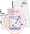 |
Fig. 1. Comparison of the ALMA coverage (red isocontours at primary beam attenuation levels of 0.8, 0.6, 0.4, and 0.2) with those of HDFS (WFPC2/F814W; background grey map) and MUSE3D (1 × 1 arcmin2 blue region). The blue stars and circles indicate the positions of the group members at zspec = 1.284 and 4.699, respectively (two of the high-redshift members lie too close to each other for their two circles to be distinguished). The HDFS imaging was aligned with Gaia-DR3 reference (Gaia Collaboration 2023) making use of three stars in the field (black diamonds) at RA, Dec = 22:32:50.513, −60:34:00.94 (used for the MUSE Slow Guiding System); 22:32:56.999, −60:34:05.82 (brightest star in the field); and 22:32:50.513, −60:32:18.83. The image is oriented such that north is up, and west is to the right. |
Adopted coordinates for the ALMA mosaic pointing.
The ALMA spectral tuning was set to the frequency division mode (FDM) setup in band 3 with four 1.875 GHz wide spectral windows (SPWs; i.e. a total continuum bandwidth of 7.464 GHz). The SPWs are centred at 87.00, 88.86, 99.06, and 100.93 GHz (νLO1 = 93.96 GHz; λ = 3.2 mm). Each SPW has 240 channels with an effective spectral resolution of 8.197 MHz (∼24 km/s at 100.93 GHz). Table 2 summarises the coverage of potential transitions from MUSE-identified galaxy groups by the single spectral setup of our observations. The tuning was chosen such that CO transitions were optimally covered towards two galaxy groups identified by MUSE. Specifically, the CO (2-1) and (5-4) transitions of the groups identified by Bacon et al. (2015) at z = 1.284 (nine members) and 4.699 (six members) were redshifted to the highest-frequency SPW in the dataset (Figure 2). Moreover, [CI] (3P1 − 3P0) at z = 4.699 is redshifted to the lowest-frequency SPW. Nevertheless, different transitions of other galaxy groups might also be covered by the other SPWs, but the observation setup is not ideal for either of the two additional groups. Either the long-baseline configurations might resolve out extended emission from the members of the zspec = 0.172 group, or the systemic velocity uncertainty of the members within the zspec = 3.013 group combined with the velocity spread of the group causes the CO transitions to fall outside our spectral coverage. In the end, we were only able to identify CO emission from the members of the group at zspec = 1.284, as detailed below.
Covered galaxy groups identified by MUSE.
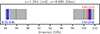 |
Fig. 2. Spectral tuning used in the survey, chosen to target the transitions CO (2-1) and (5-4) towards the two galaxy groups identified by the MUSE 3D survey at z = 1.284 and 4.699, with nine and six reported members, respectively (the vertical lines correspond to each member). For the z = 4.699 group, the [CI] (1-0) transition is also covered. |
2.3. Observing strategy and calibration
The observations were carried out from 2023 September 05th to 2023 November 30th. During this period, the 12 m array was reconfigured to cover ALMA configurations C-9 to C-7 (see Cortes et al. 2022, for ALMA technical details). During the period between 2023 October 30th and 2023 November 27th, the array was in a hybrid configuration, between C-8 and C-7, which we refer to as C-7hybrid (or C-7h) throughout. Table 3 lists the number of execution blocks (EBs) in each distinct configuration, and further detail is given in Appendix A.
Summary of the ALMA scheduling EBs per configuration.
The phase calibration for our science target was made with the quasar J2239-5701 (3.6 deg away) with a cycle time of 54 s that was unchanged during the period within which the project was observed. The check source was J2207-5346 (5.4 deg away from J2239-5701). Finally, in each execution, the bandpass and flux calibration made use of a single calibrator source (J2357-5311 or J2258-2758).
Each execution was expected to run for 1.8 h (∼50 min on-source). Overall, the total of 70 observing executions at ALMA resulted into 61 h of effective time on-source, distributed over the four pointings. The data were calibrated with the ALMA pipeline version 2022.2.0.68 (Hunter et al. 2023) and CASA 6.4.1.12 (CASA Team 2022), which took the equivalent of 48 days of single-cluster-node continuous computing time to process. Appendix A provides more detailed information on each of the considered EBs.
2.4. Survey depth and noise properties
Since observations were executed in a range of configurations, we assessed the survey noise properties on a subset of 47 EBs with common baseline ranges (from 70 − 90 m to 8.3 km) to avoid the contribution from additional baseline coverage (namely at > 8.3 km scales). We first determined the noise RMS on a per-EB basis, and we then sorted it accordingly. The sensitivity assessment was then performed on continuum maps with an incremental number of EBs of 1, 2, 4, 8, 16, 32, and 47 EBs (starting from the lowest-noise EB and gradually adding the next EBs in line). We only created dirty maps (without deconvolution) using natural weighting (i.e. no image weights were applied, which resulted in highest sensitivity) with the same pixel and image size. Figure 3 shows the sensitivity as a function of time on-source (TOS) and compares it with the expectation from the radiometric equation (see Equation (9.8) in Section 9.2.1 in Cortes et al. 2025, lower region bound) and the ALMA sensitivity calculator4 (upper region bound). The noise expectation from the latter is slightly higher (+10%) than the former. The natural-weighted map combining 47 EBs reaches RMS = 1.7 μJy/beam, and the final continuum map combining all observed 70 EBs reaches RMS = 1.4 μJy/beam. The map created by the standard ALMA pipeline with robust parameter equal to 0.5 reaches 1.9 μJy/beam.
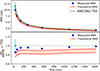 |
Fig. 3. Sensitivity (noise RMS) as a function of integration time as measured in a sensitivity-ordered sub-sample of 47 EBs with a fixed range of baseline length. The upper plot shows the measured image RMS (blue squares) and the theoretical RMS expected from the radiometric equation and ALMA sensitivity calculator (red shaded region) vs. TOS. The cyan datapoint with the error bar shows the median RMS and the standard deviation of the per-EB continuum map RMS values. The solid green curve shows the expected RMS decrease from this median datapoint with a simple scaling by the square root of the exposure time. The lower plot shows the same information normalised by the solid green curve in the upper plot. |
2.5. Angular scales
The continuum-synthesised beam obtained by combining data over all spectral windows and imaging with Briggs weighting (robust = 0.5; Briggs 1995) is 0.13″ × 0.15″ at PA = 33 deg. At zspec = 1.284 and 4.699, this implies intrinsic spatial scales of 1.2 kpc and 0.9 kpc, respectively. Throughout this paper, we also make reference to data cubes and continuum maps imaged with natural weighting, which results in a larger synthesised beam of 0.22″ × 0.19″ at PA = 49 deg in the continuum map. Natural weighting is preferred because in addition to its higher sensitivity, it is also more desirable for a detection in the angular scale range.
When several configurations are covered regardless of tailored observing times (see Section 7.8 of Cortes et al. 2022), as in the case of our dataset, the best possible baseline length distribution (BLD) for the most Gaussian beam shape is not achieved. An analysis using the tools developed by Petry et al. (2024) showed that the achieved BLD deviated from an ideal shape for the same angular resolution of ∼0.12″ and a maximum recoverable scale of 1″. Figure 4 (left panel) shows that the observed BLD (blue) has an excess sensitivity at the shortest and longest baseline lengths and corresponding sensitivity deficits at intermediate baseline lengths between ∼1500 m and 5000 m. This is partially a design feature of the ALMA configurations and partially due to the combination of configurations, but is not expected to affect the imaging reconstruction negatively. The excess at short baselines is even beneficial for the detection aspect of the experiment. On the other hand, as already indicated by the near-circular beam, the right panel of the same figure shows that the azimuthal coverage of our observations is almost perfectly homogeneous (with only a very slight under-exposure at azimuth 0–45° and baseline lengths ∼2000–4000 m). This is a result of the approximately symmetric array configurations and the wide range of observing hour angles.
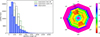 |
Fig. 4. Assessment of the quality of the uv coverage of our combined data using the tools developed by Petry et al. (2024). (Left) Observed and expected 1D BLDs, i.e. histogram of the baseline lengths of the visibilities for the representative frequency channel (87 GHz) of the dataset (blue) and the corresponding expected histograms for the ideal shape to achieve the most Gaussian PSF given an angular resolution range ±20% around the nominal value of ∼0.13″ (green and grey histograms). (Right) Plot of the ratio of the observed and expected BLD in 2D, i.e., also showing the baseline orientation. A value of 1.0 indicates that observation and expectation agree exactly. Higher values indicate an over-exposure, and lower values show an under-exposure. |
Overall, following the prescription detailed by Petry et al. (2024) and using the ASSESS_MS 3 software (Petry et al. 2025), we found the following statistics on the final combined MS (scales are referenced to 87 GHz):
-
the longest baseline is 14.9 km,
-
the shortest baseline is 29 m,
-
the shortest and longest expected BL for a Gaussian beam shape are 152 m and 7283 m,
-
the 80th percentile baseline length (L80) is 2863 m, which is equivalent to an angular resolution (AR) = 0.14″,
-
the 5th percentile baseline length (L05) is 258 m, which is equivalent to a maximum recoverable scale (MRS) of 2.7″,
-
an almost homogeneous sensitivity is reached for the entire baseline length range,
-
the baseline orientation is sufficiently homogeneous in all baseline ranges.
3. Results
3.1. Continuum map
In order to identify continuum detections at the observed wavelength of 3.2 mm, we focused on the natural-weighted primary-beam (PB) uncorrected map with a 0.5″uv taper, for which the average map noise RMS is 2.4 μJy/beam, and the lowest negative peak in the map is −10.5 μJy/beam. As a result, we conservatively only considered regions in the map as detections with peak fluxes above 10.5 μJy/beam (i.e. > 4.4 σ; resulting in fewer than one false detection in our map) and within the region in which the PB attenuation factor is ≳0.5. Table 4 lists the three identified continuum detections and fitting results from the CASA task imfit. Only ID 1 of the three detected sources is associated with a Spitzer/IRAC detection (Appendix B) and also shows a faint counterpart in HDFS/F814W imaging (i814 = 25.5 ± 0.03 AB; Casertano et al. 2000). Moreover, multi-frequency radio observations (Huynh et al. 2005, 2007) with the Australia Telescope Compact Array (Wilson et al. 2011) show clear detections from ∼1 mJy (S/N = 104) at 1.4 GHz down to ∼0.2 mJy (S/N = 19) at 8.7 GHz. Together with the ALMA detection, we measure a spectral index of α ∼ −0.8, which is consistent with synchrotron emission. It is beyond the scope of this paper to push the continuum detections beyond simple point or compact sources towards extended structures or into the noise limit.
Continuum source detections.
3.2. Line emitters
As mentioned in Section 2.2, at least two galaxy groups are identified by MUSE (Bacon et al. 2015) whose specific CO transitions are covered by the adopted tuning.
With a special focus on the highest-frequency spectral window and using a natural-weighted cube, we conducted a two-step line search of the velocity-integrated (moment-0) maps towards the location of the MUSE-detected sources at the frequency at which the CO line is expected to be redshifted based on the redshift reported by MUSE. Briefly, we first started building moment-0 maps within ±600 km/s around the expected line frequency. This value was chosen to accommodate potentially broad line profiles as well as significant offsets with respect to the redshift reported by MUSE. This is quite important because the z = 4.7 group is identified via the Lyman-α line alone, and this line is known to present significant velocity offsets with respect to the systemic redshift of the host galaxy (e.g., Verhamme et al. 2018). When a significant detection in the moment-0 map was obtained (i.e. above five times the median absolute deviation, MAD), we extracted a preliminary spectrum of the source within the significantly detected region. This spectrum was then used to fine-tune the frequency range within which a new moment-0 map was to be retrieved. The updated significantly detected region was subsequently used to extract the final spectrum that was used to determine the spectral range within which the velocity and dispersion maps were to be obtained. The results are displayed in Figures 5 through 9, where we report the CO (2-1) line detections towards five out of the nine group members detected by MUSE. Furthermore, we present in Figure 10 one serendipitous detection near B15-114 that itself does not show CO (2-1) emission.
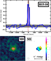 |
Fig. 5. CO (2-1) emission towards B15-10. The cube used for the analysis was imaged with natural weighting and with a smoothing of four channels (i.e. resulting in a spectral resolution of ∼90 km/s). We present the detection spectrum in the top panel, and the velocity-integrated flux map (moment-0, M0) and the velocity map (moment-1, M1) are shown in the bottom left and right panels, respectively. Both maps have the same size (i.e., 3.4″ wide, or ∼29 kpc). The moment-0 contours are overlaid on both maps (solid black contours indicate levels at |

Table 5 reports the observed properties of each of the six line detections. The conversion of the CO (2-1) luminosity (L′CO(2 − 1)) and molecular gas mass (MH2) was firstly made using a factor of 0.75 ± 0.11 to turn L′CO(2 − 1) into CO (1-0) luminosities (Boogaard et al. 2020), and secondly, using a CO-to-H2 conversion factor of αCO = 4 M⊙/(K.km/s.pc2) (including helium; Dunne et al. 2022). We acknowledge that the underlying assumption of this value is that these galaxies are metal enriched (Z/Z⊙ ≳ 0.5; Dunne et al. 2022). Although no metallicity estimates are available for the members in the targeted group, we adopted the stellar masses reported by Contini et al. (2016) for four of the group members (10, 13, 27, and 35 with log10(M* [M⊙]) = 9.9 − 10.8, assuming a Chabrier 2003 initial mass function) and converted them into metallicities assuming the mass-metallicity relation. Based on observations (adopting local samples, e.g., Blanc et al. 2019) or theory (considering redshift evolution, e.g., Ma et al. 2016), we obtained  or 0.3–0.6, respectively. This shows that the sample mostly lies still within the applicable metallicity range.
CO (2-1) line detections towards the galaxy group at zspec = 1.284.
We finally note that half of the detected sample shows MH2 values at and below the H2 mass limit reached by the deepest ALMA line surveys at similar redshifts so far (MH2 = 0.63 − 9.7 × 10¹⁰ M⊙ at 1.09 < z < 1.55; Decarli et al. 2019).
We also fitted the detected lines with single-component Gaussian profiles. The best-fit solutions are shown in the spectra in the top panels in Figures 5 through 10. The best fit is shown by the thick line for the raw spectral resolution (24 km/s) cube and by the dashed line for the four-channel-smoothed cube. Table 6 reports the fitting results, and Table 7 lists the difference in the redshift determination between CO and optical estimates.
Gaussian fit results to the line detections.
Redshift comparison between ALMA and MUSE.
The diversity found in this group is clear overall, as is the proximity of the galaxies to each other. For reference, the brightest three galaxies we found (B15-10, 15, and 27) lie within ∼50 to ∼140 kpc (projected) from each other, and Contini et al. (2016) reported evidence of low surface brightness emission between B15-10 and B15-27, which indicates that these two galaxies might already have interacted. B15-27 is an interesting case on its own when we compare its dynamical map with that based on [OII]3729 (Contini et al. 2016) and the rest-frame UV map (Appendix C). While the rotation pattern of this galaxy is very clear, the CO(2-1) velocity-integrated flux centroid is clearly offset from its rest-frame UV counterparts. The latter even appears to show a very disturbed system, and the [OII]3729 velocity map is clearly extended to the west. This agrees with the location of one or two close-by companion clumps detected in CO(2-1) (∼5 kpc away and offset in velocity up to −500 km/s; one of the clumps might show a rotation pattern as well). We also found indications for a higher-velocity feature (at 100–150 km/s) north-east of B15-35, but despite the clear alignment between the velocity patterns between ionised and molecular gas, Contini et al. (2016) reported no significant evidence of this feature in the [OII]3729 velocity map. Because of the multi-wavelength richness towards the detected sources, we defer a more complete dynamical analysis to a future work.
Moreover, we found a significant (σ ∼ 6) serendipitous CO (2-1) detection north-east of B15-114 (which we label ALMA-114). B15-114 itself remains undetected in CO (2-1), but its MUSE [OII]-derived redshift of zspec = 1.2844 is very close to the redshift obtained for this companion, zspec = 1.28349 ± 0.00059.
Finally, we did not detect any line emission towards the other groups listed in Table 2 or within the whole field. It is beyond the scope of this paper to pursue a more detailed detection analysis (e.g. stacking), especially towards the high-redshift group for which the systemic redshifts are uncertain. We note that the shallower but wider ASPECS-3mm survey (Decarli et al. 2019) reported no CO(5-4) detections at z > 4 either. The COLDz survey (Riechers et al. 2019) reported detections of CO(2-1) at z ∼ 5 towards three previously known dusty star-forming galaxies (DSFGs). The CO(5-4) line fluxes reported therein for the same galaxies would have been detectable in our survey. This also shows that this MUSE-identified galaxy group does not include such DSFGs within 200 kpc (projected) from the identified group members. More reliable conclusions on the source properties for this group require the knowledge of the systemic redshift, which the Lyman-α line emission does not guarantee.
We also made use of the source-finding application (version 2.5.1, SoFiA-2; Serra et al. 2015; Westmeier et al. 2021)5 to blindly search for emission lines in each of the four spectral windows. Only four of the detections reported before were automatically considered significant by SoFiA-2, however, which shows that in this case, it is better to know where the sources are located with an initial guess of the systemic redshift.
3.3. Cosmic molecular gas-mass density in group environments
Despite the small projected survey size (1 arcmin2), we attempted to estimate the cosmic molecular gas density (ρH2) from the galaxy population in group environments. We used this [OII]3727, 3729-identified group at zspec = 1.284 as reference, which we assumed to be representative.
We adopted the 1/Vmax formalism (Schmidt 1968). The zmin and zmax were estimated with two slightly different approaches. The consideration of the MUSE sensitivity profile (or passband) from 480 to 930 nm is common to both limits. This allowed us to take the sensitivity dips (that translate to reduced completeness; Drake et al. 2017) in the whole spectral range into account. We obtained it from the VLT/MUSE exposure time calculator, which emulates the observing conditions of the MUSE observations taken around 29 July 2014. The obtained trend was smoothed to the line FWHM reported in Table 6.
We recall that the redshift estimate of a source for which only the [OII] doublet is detected depends on the resolution of the doublet (which MUSE is capable of) and on the detection of the fainter line at a rest frame of 3727 Å. We therefore adopted it as reference and a 3729–3727 Å line ratio of 1.3 (Kaasinen et al. 2017) because only the combined flux of the doublet was reported by Bacon et al. (2015).
The zmin was estimated only based on the MUSE coverage of [OII]3727, 3729 together with the sensitivity profile, guaranteeing an S/N > 5, which resulted in zmin = 0.289. On the other hand, zmax was estimated based on the [OII]3727, 3729 and CO (2-1) integrated-line fluxes. Briefly, zmax was limited to MUSE coverage of [OII]3727, 3729 at z ∼ 1.49. On a case-by-case basis, this value might be lower, depending on the observed [OII]3727, 3729 and CO (2-1) properties.
We adopted two additional corrections. The first correction is related to the strong sensitivity dips in the MUSE sensitivity profile (e.g. at ∼860 − 870 nm), which for a narrow redshift range might result in a non-detection (hence lower completeness; Drake et al. 2017), but at higher redshifts is considered detectable again. To account for this, we corrected the full initial volume (from zmin to zmax) for the fraction of bins in this range that would yield a detection. This value was found to be between 0.924 and 0.975, and it is only a small correction in this case. In the second correction, we note that Bacon et al. (2015) identified groups as those with three or more members, hence this group would be identified as such until the last three brightest members would be detectable. In this case, they would be B15-10, B15-15, and B15-35, and zmax was capped at z = 1.4935.
We did not attempt to correct for the intrinsic evolution of this group, in other words, for the fact that the star formation rate density (hence [OII] emission related to star formation) strongly declines from z = 1.49 to z = 0.289. Our ability to identify these types of numerous groups might therefore decline as well. We note, however, that this would further increase the reported molecular gas-mass volumetric density.
Finally, we considered cosmic variance and low-number statistics. To account for this, we followed Trenti & Stiavelli (2008) and used their calculator Version 1.03 (24 July 2020) https://www.ph.unimelb.edu.au/~mtrenti/cvc/CosmicVariance.html to compute the total fractional error (Poisson uncertainty and cosmic variance) on the number counts based on redshift range, field size, and number of sources. This value is about 0.5 in our case. Based on the low number statistics, whenever we refer to the statistical uncertainty, it was estimated as  6, where the negative and positive signs refer to the lower and upper errors, respectively.
Nevertheless, despite what we described in the previous two paragraphs, we highlight that other surveys conducted with MUSE down to similar or deeper levels (Bacon et al. 2017, 2023; Fossati et al. 2019) also show groups at similar redshifts with many members. For instance, Fossati et al. (2019) reported two groups with more than ten members at zspec ∼ 0.678 and 1.053. The catalogues provided by Bacon et al. (2023) based on the deepest MUSE survey ever taken also show two clear redshift peaks at zspec ∼ 0.659 and 1.089. Bacon et al. (2015) also reported a group with seven members at zspec ∼ 0.564 in addition to the group that is the focus of this work. This therefore appears to show that [OII]-identified groups might be a common observable at an age of the Universe between 5.5 and 7.5 Gyr.
The molecular hydrogen mass function (MF) obtained for this group at zspec = 1.284 is presented in Figure 11. We compared this result with work from the literature that is representative of the galaxy population in the field environment by (Decarli et al. 2019, 2020, 1.0 < z < 1.7), (Lenkić et al. 2020, 1.2 < z < 1.7), and (Messias et al. 2024, 1.0 < z < 1.8). We additionally show the results reported by Berta et al. (2013), who adopted two different scalings with the star formation rate to derive the H2 MF at different redshift ranges in between 0.2 < z < 2.0. All data were made consistent by adopting the same CO-to-H2 conversion factor (αCO = 4 including helium fraction; Dunne et al. 2022) and cosmology. The figure shows that group and field environments apparently show similar MFs (within the current uncertainties), but, more noticeably, our survey reaches almost by 0.5 dex deeper in molecular mass at these redshifts than ASPECS (Decarli et al. 2019, 2020) and Berta et al. (2013). At these levels, the results show that the molecular gas MF still increases with decreasing luminosity, but is still consistent with the flat light-end of the H2 MF observed as late as 0.2 < z < 0.6.
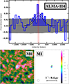 |
Fig. 10. Same as in Figure 5, but for ALMA-114. We detect no emission towards the location of B15-114, but in the north-east towards a source labelled ALMA-114 in this work. The moment-0 map (centred on the new source detection) shows a significant detection (S/N ∼ 6) associated with a broad CO (2-1) line detection, very close in redshift to B15-114 (indicated with the vertical dotted line in the spectrum). The lower S/N feature in the south-west of the image is not associated with the B15-114 source, which is instead located 0.5″ south of it. |
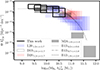 |
Fig. 11. Molecular gas-mass function derived from the observed group at zspec = 1.284 compared to works in the literature by (Decarli et al. 2019, 2020, D19 and D20, at 1.0 < z < 1.7), (Lenkić et al. 2020, L20, at 1.2 < z < 1.7), and (Messias et al. 2024, M24, at 1.0 < z < 1.8). The results by Berta et al. (2013, different line types for different redshift ranges) were derived from empirical scaling relations, instead of inferring MH2 from CO as the previously cited works. The empty boxes show the results from our study. These are 0.5 dex wide in molecular gas mass (centred at each step of 0.25 dex), and the vertical width shows the statistical uncertainty. |
Figure 12 reports the cosmic molecular gas-mass density in group environments compared to results from the literature either based on surveys that directly detected CO rotational transitions (Decarli et al. 2020; Messias et al. 2024, grey-line boxes) or on sub-millimeter continuum relations (Scoville et al. 2017, continuous grey-line region). We highlight that the molecular gas-mass densities recovered by this survey7 are comparable to those of blind CO surveys in the literature. The implications for this are discussed in Section 4.
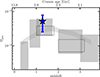 |
Fig. 12. Cosmic molecular gas-mass density in group environments derived using the group identified by MUSE and detected by ALMA in CO (2-1) at z = 1.284 (blue data point and error bar). For reference, literature estimates are also included. The CO-derived estimates reported by Decarli et al. (2020) from z = 0.271 to 4.475 appear as filled grey boxes, and those at 1 ≲ z ≲ 3 reported by Messias et al. (2024) appear as empty boxes. The sub-millimeter continuum derived trend from Scoville et al. (2017) is displayed as a continuous filled grey region. The cosmic mass density is plotted as the ratio to the critical cosmic density. |
4. Conclusions
We described a 1 × 1 arcmin2 deep single-tuning survey at sub-arcsecond scales conducted by ALMA in the Hubble Deep Field South (HDFS). The spectral tuning was especially chosen to trace CO transitions in galaxies belonging to two groups identified by MUSE at zspec = 1.284 and 4.699 (Section 2).
This survey was conducted as an ALMA observatory project (filler in nature) that resulted in a total time on source of 61 h, which yielded a continuum sensitivity of RMS = 1.4 μJy/beam (adopting natural weighting; Section 2.4). The unprecedented uv coverage range for a millimeter survey yields a spatial resolution of 0.13″ × 0.15″ (adopting Briggs weighting with robust = 0.5) and maximum recoverable scales of 1–2 arcsec (Section 2.5).
We reported CO (2-1) detections toward five out of the nine members of the galaxy group at zspec = 1.284 and further identified a previously unknown member of the same group without an optical or NIR counterpart (Section 3.2). The expected molecular gas masses of half of the sample detected by ALMA are at and below the mass cut reached by previous deep spectral-scan surveys covering similar redshifts. The gas detections are highly diverse, and no two sources are alike in terms of their size and dynamical states. Only one source shows a smooth rotation pattern, but also evidence of two satellite features, and it is clearly offset with respect to its rest-frame UV-optical emission. The observed line widths vary, and the sizes vary from point-like to 10 kpc.
Based on the CO (2-1) detections towards this group, we attempted to estimate the molecular gas-mass function (MF) and the cosmic molecular gas-mass density (ΩH2) in the group environments. We found evidence that the MFs of the group environments cannot be distinguished from those of field galaxies (within the observed uncertainties), and at the survey depth, the MFs show no indication of a decrease in number density with decreasing molecular gas, but are still consistent with the flat light-end of the MFs observed at z < 1. The recovered ΩH2 is comparable to that of populations with larger H2 contents found in wider and shallower surveys. Because the projected survey size is small, we acknowledge that there is room for a large uncertainty in the result, but we note that this group does not appear to be a rare observable at similar redshifts in other deep MUSE fields. We are therefore confident that our result might indeed be representative of group environments when the Universe was approximately half its current age (Section 3.3). Moreover, this should be evidence that our current knowledge of ΩH2 and its evolution back in time is still rather incomplete at z > 1. In other words, we still do not know when ΩH2 peaked, and any estimate of how much it has decreased since z ∼ 1 − 2 needs to be taken as a lower limit. Nevertheless, the potential no-evolution scenario of the H2 MF light-end (MH2 ≲ 1010 M⊙) between z ∼ 0.2 and ∼1.3 might help us to compensate for the increased incompleteness that affects current surveys at earlier cosmic times.
Finally, we detected three significant sources in the continuum map (S/N > 4.4σ), only one of which shows multi-wavelength counterparts from rest-frame UV to radio frequencies. The other two continuum detections are expected to be thermal in nature because a synchrotron SED is expected to result in clear detections in existing data at 1.4 GHz.
Acknowledgments
This paper makes use of the following ALMA data: ADS/JAO.ALMA#2022.A.00034.S. ALMA is a partnership of ESO (representing its member states), NSF (USA) and NINS (Japan), together with NRC (Canada), NSTC and ASIAA (Taiwan), and KASI (Republic of Korea), in cooperation with the Republic of Chile. The Joint ALMA Observatory is operated by ESO, AUI/NRAO and NAOJ. The National Radio Astronomy Observatory is a facility of the National Science Foundation operated under a cooperative agreement by Associated Universities, Inc. This research made use of IPYTHON (Perez & Granger 2007), NUMPY (van der Walt et al. 2011), MATPLOTLIB (Hunter 2007), SCIPY (Virtanen et al. 2020), ASTROPY (a community-developed core PYTHON package for Astronomy, Astropy Collaboration 2013), TOPCAT (Taylor 2005), APLpy (an open-source plotting package for Python, Robitaille & Bressert 2012). The team appreciates the constructive feedback provided by the anonymous referee that pushed us toward a significantly improved version of the manuscript.
References
- Astropy Collaboration (Robitaille, T. P., et al.) 2013, A&A, 558, A33 [NASA ADS] [CrossRef] [EDP Sciences] [Google Scholar]
- Bacon, R., Accardo, M., Adjali, L., et al. 2010, SPIE Conf. Ser., 7735, 773508 [Google Scholar]
- Bacon, R., Brinchmann, J., Richard, J., et al. 2015, A&A, 575, A75 [NASA ADS] [CrossRef] [EDP Sciences] [Google Scholar]
- Bacon, R., Conseil, S., Mary, D., et al. 2017, A&A, 608, A1 [NASA ADS] [CrossRef] [EDP Sciences] [Google Scholar]
- Bacon, R., Brinchmann, J., Conseil, S., et al. 2023, A&A, 670, A4 [NASA ADS] [CrossRef] [EDP Sciences] [Google Scholar]
- Berta, S., Lutz, D., Nordon, R., et al. 2013, A&A, 555, L8 [NASA ADS] [CrossRef] [EDP Sciences] [Google Scholar]
- Bianconi, M., Smith, G. P., Haines, C. P., et al. 2018, MNRAS, 473, L79 [CrossRef] [Google Scholar]
- Blanc, G. A., Lu, Y., Benson, A., Katsianis, A., & Barraza, M. 2019, ApJ, 877, 6 [NASA ADS] [CrossRef] [Google Scholar]
- Boogaard, L. A., van der Werf, P., Weiss, A., et al. 2020, ApJ, 902, 109 [NASA ADS] [CrossRef] [Google Scholar]
- Briggs, D. S. 1995, Ph.D. Thesis, New Mexico Institute of Mining and Technology [Google Scholar]
- Brown, R. L., Wild, W., & Cunningham, C. 2004, Advances in Space Research, 34, 555 [Google Scholar]
- CASA Team (Bean, B., et al.) 2022, PASP, 134, 114501 [NASA ADS] [CrossRef] [Google Scholar]
- Casertano, S., de Mello, D., Dickinson, M., et al. 2000, AJ, 120, 2747 [NASA ADS] [CrossRef] [Google Scholar]
- Chabrier, G. 2003, PASP, 115, 763 [Google Scholar]
- Contini, T., Epinat, B., Bouché, N., et al. 2016, A&A, 591, A49 [NASA ADS] [CrossRef] [EDP Sciences] [Google Scholar]
- Cortes, P. C., Remijan, A., Hales, A., et al. 2022, ALMA Technical Handbook Cycle 9 (ALMA Doc. 9.3, version 1.0), https://almascience.eso.org/documents-and-tools/cycle9/alma-technical-handbook [Google Scholar]
- Cortes, P. C., Remijan, A., Hales, A., et al. 2025, ALMA Technical Handbook Cycle 12 (ALMA Doc 12.3, version 1.0), https://almascience.eso.org/documents-and-tools/cycle12/alma-technical-handbook [Google Scholar]
- Decarli, R., Walter, F., Aravena, M., et al. 2016, ApJ, 833, 69 [Google Scholar]
- Decarli, R., Walter, F., Gónzalez-López, J., et al. 2019, ApJ, 882, 138 [Google Scholar]
- Decarli, R., Aravena, M., Boogaard, L., et al. 2020, ApJ, 902, 110 [Google Scholar]
- Drake, A. B., Garel, T., Wisotzki, L., et al. 2017, A&A, 608, A6 [NASA ADS] [CrossRef] [EDP Sciences] [Google Scholar]
- Dunlop, J. S., McLure, R. J., Biggs, A. D., et al. 2017, MNRAS, 466, 861 [Google Scholar]
- Dunne, L., Maddox, S. J., Papadopoulos, P. P., Ivison, R. J., & Gomez, H. L. 2022, MNRAS, 517, 962 [NASA ADS] [CrossRef] [Google Scholar]
- European Southern Observatory. 1998, The VLT White Book [Google Scholar]
- Ferguson, H. C., Dickinson, M., & Williams, R. 2000, ARA&A, 38, 667 [Google Scholar]
- Fossati, M., Fumagalli, M., Lofthouse, E. K., et al. 2019, MNRAS, 490, 1451 [NASA ADS] [CrossRef] [Google Scholar]
- Franco, M., Elbaz, D., Béthermin, M., et al. 2018, A&A, 620, A152 [NASA ADS] [CrossRef] [EDP Sciences] [Google Scholar]
- Fujita, Y. 2004, PASJ, 56, 29 [NASA ADS] [Google Scholar]
- Gaia Collaboration (Vallenari, A., et al.) 2023, A&A, 674, A1 [NASA ADS] [CrossRef] [EDP Sciences] [Google Scholar]
- Hatsukade, B., Kohno, K., Umehata, H., et al. 2016, PASJ, 68, 36 [NASA ADS] [CrossRef] [Google Scholar]
- Hatsukade, B., Kohno, K., Yamaguchi, Y., et al. 2018, PASJ, 70, 105 [Google Scholar]
- Hill, R., Scott, D., McLeod, D. J., et al. 2024, MNRAS, 528, 5019 [NASA ADS] [CrossRef] [Google Scholar]
- Hill, R., Polletta, M. d. C., Béthermin, M., et al. 2025, A&A, 698, A204 [NASA ADS] [CrossRef] [EDP Sciences] [Google Scholar]
- Hunter, J. D. 2007, Comput. Sci. Eng., 9, 90 [NASA ADS] [CrossRef] [Google Scholar]
- Hunter, T. R., Indebetouw, R., Brogan, C. L., et al. 2023, PASP, 135, 074501 [NASA ADS] [CrossRef] [Google Scholar]
- Huynh, M. T., Jackson, C. A., Norris, R. P., & Prandoni, I. 2005, AJ, 130, 1373 [Google Scholar]
- Huynh, M. T., Jackson, C. A., & Norris, R. P. 2007, AJ, 133, 1331 [Google Scholar]
- Kaasinen, M., Bian, F., Groves, B., Kewley, L. J., & Gupta, A. 2017, MNRAS, 465, 3220 [Google Scholar]
- Kennicutt, R. C., Jr. 1998, ApJ, 498, 541 [Google Scholar]
- Kneissl, R., Polletta, M. d. C., Martinache, C., et al. 2019, A&A, 625, A96 [NASA ADS] [CrossRef] [EDP Sciences] [Google Scholar]
- Lenkić, L., Bolatto, A. D., Förster Schreiber, N. M., et al. 2020, AJ, 159, 190 [CrossRef] [Google Scholar]
- Ma, X., Hopkins, P. F., Faucher-Giguère, C.-A., et al. 2016, MNRAS, 456, 2140 [NASA ADS] [CrossRef] [Google Scholar]
- Magnelli, B., Boogaard, L., Decarli, R., et al. 2020, ApJ, 892, 66 [NASA ADS] [CrossRef] [Google Scholar]
- Messias, H., Guerrero, A., Nagar, N., et al. 2024, MNRAS, 533, 3937 [Google Scholar]
- Miller, T. B., Chapman, S. C., Aravena, M., et al. 2018, Nature, 556, 469 [CrossRef] [Google Scholar]
- Oteo, I., Ivison, R. J., Dunne, L., et al. 2018, ApJ, 856, 72 [Google Scholar]
- Perez, F., & Granger, B. E. 2007, Comput. Sci. Eng., 9, 21 [Google Scholar]
- Petry, D., Díaz Trigo, M., Kneissl, R., et al. 2024, SPIE Conf. Ser., 13098, 130980P [Google Scholar]
- Petry, D., Diaz Trigo, M., Kneissl, R., et al. 2025, https://doi.org/10.5281/zenodo.16682282 [Google Scholar]
- Planck Collaboration VI. 2020, A&A, 641, A6 [NASA ADS] [CrossRef] [EDP Sciences] [Google Scholar]
- Riechers, D. A., Pavesi, R., Sharon, C. E., et al. 2019, ApJ, 872, 7 [Google Scholar]
- Robitaille, T., & Bressert, E. 2012, Astrophysics Source Code Library [record ascl:1208.017] [Google Scholar]
- Schmidt, M. 1959, ApJ, 129, 243 [NASA ADS] [CrossRef] [Google Scholar]
- Schmidt, M. 1968, ApJ, 151, 393 [Google Scholar]
- Scoville, N., Lee, N., Vanden Bout, P., et al. 2017, ApJ, 837, 150 [Google Scholar]
- Serra, P., Westmeier, T., Giese, N., et al. 2015, MNRAS, 448, 1922 [Google Scholar]
- Taylor, M. B. 2005, ASP Conf. Ser., 347, 29 [Google Scholar]
- Trenti, M., & Stiavelli, M. 2008, ApJ, 676, 767 [Google Scholar]
- van der Walt, S., Colbert, S. C., & Varoquaux, G. 2011, Comput. Sci. Eng., 13, 22 [Google Scholar]
- Verhamme, A., Garel, T., Ventou, E., et al. 2018, MNRAS, 478, L60 [Google Scholar]
- Virtanen, P., Gommers, R., Oliphant, T. E., et al. 2020, Nat. Methods, 17, 261 [Google Scholar]
- Vulcani, B., Poggianti, B. M., Fritz, J., et al. 2015, ApJ, 798, 52 [Google Scholar]
- Vulcani, B., Treu, T., Nipoti, C., et al. 2017, ApJ, 837, 126 [NASA ADS] [CrossRef] [Google Scholar]
- Walter, F., Decarli, R., Aravena, M., et al. 2016, ApJ, 833, 67 [Google Scholar]
- Walter, F., Carilli, C., Neeleman, M., et al. 2020, ApJ, 902, 111 [Google Scholar]
- Westmeier, T., Kitaeff, S., Pallot, D., et al. 2021, MNRAS, 506, 3962 [NASA ADS] [CrossRef] [Google Scholar]
- Wilson, W. E., Ferris, R. H., Axtens, P., et al. 2011, MNRAS, 416, 832 [Google Scholar]
There are slight differences between the values reported in the right column in Table 2 in Planck Collaboration VI (2020) and the ASTROPY.COSMOLOGY.PLANCK18 package. Specifically, for ΩM, with reported values of 0.3111 and 0.30966, respectively. The difference is related to the parameter definition, namely the inclusion or exclusion of massive neutrinos (as reported in issue 10957 in GITHUB).
More information on observatory projects: https://almascience.eso.org/alma-data/observatory-projects
This alternative is proposed by the Collider Detector at Fermilab Statistics Committee and also accessible within the ASTROPY.STATS package, in the function POISSON_CONF_INTERVAL, by setting INTERVAL = ‘PEARSON’.
We note that removing ALMA-114 from the analysis would only reduce ρH2 by 2%.
Appendix A: Observation details
Table A.1 lists the 70 execution blocks (EBs) used to build the continuum maps and cubes. The columns contain: EB unique identifiers (UIDs), date of observation, number of antennas in the array, configuration, minimum and maximum baseline, J-name of the bandpass calibrator (also used for flux calibration), phase calibrator, and time on science target.
Details of the observed EBs.
Appendix B: Comparison with near-IR emission
In Figure B.1, we compare the ALMA 3 mm continuum map (natural-weighted with a 0.5” uv-taper as used for continuum source detection) with Spitzer/IRAC-3.6 μm map. Only one of the three reliable continuum detections has a match with an IRAC-detected source. Moreover, we note that we do find evidence for a ∼3σ detection (21.3 ± 6.9 μJy) towards an IRAC source at RA, Dec = 22:32:57.55, -60:33:06.2 (at a PB attenuation of 0.54). The five main line detections (Figures 5 through 9) are all detected in IRAC (rest-frame ∼1.6 μm), while the serendipitously found line emitter ALMA-114 is not. Finally, it is worth noting that the filamentary structure, with B15-10 and ALMA-114 placed at its extremes (∼20” or ∼170 kpc apart), is showing evidence of the type of environment these sources are found in.
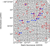 |
Fig. B.1. The natural-weighted 3mm continuum map with a 0.5” uv-taper (gray scale) with contours overlaid from the IRAC-3.6 μm map (red isocontour levels at 3, 6, and 12σ). Sources that revealed CO (2-1) line emission are marked with open blue stars, while the continuum detections reported in Table 4 are marked as blue circles. The potential 3σ continuum detection toward an IRAC source is marked with a blue square. |
Appendix C: Comparison with rest-frame UV-optical emission
In this section we provide a comparison between the CO (2-1) emission from sources within the group at zspec = 1.284 and the rest-frame UV-optical emission traced by HST imaging. Specifically the longest-wavelength WFPC2 filter F814W (λ = 827 ± 88 nm) traces λrest = 362 ± 40 nm) at zspec = 1.284. HST imaging was aligned with Gaia-DR3 (Gaia Collaboration 2023) making use of three stars in the field (details in Figure 1). Figure C.1 shows F814W maps with CO (2-1) maps overlaid on the six sources with detected CO emission. One can clearly see the spatial offset between star-formation regions traced by HST and the molecular gas emission in B15-27 and B15-35. This is especially interesting since B15-27 is the source showing the cleanest rotation pattern in the sample (see more discussion in Section 3.2). ALMA-114 is clearly undetected by HST, while its companion B15-114 is in the South-West region.
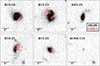 |
Fig. C.1. Comparison between HST WFPC2/F814W imaging (background gray image) and the CO (2-1) maps (red contours) for the detected sources. Cutouts are 4″ wide (∼34 kpc). The contours indicate levels at |

All Tables
All Figures
|
Fig. 1. Comparison of the ALMA coverage (red isocontours at primary beam attenuation levels of 0.8, 0.6, 0.4, and 0.2) with those of HDFS (WFPC2/F814W; background grey map) and MUSE3D (1 × 1 arcmin2 blue region). The blue stars and circles indicate the positions of the group members at zspec = 1.284 and 4.699, respectively (two of the high-redshift members lie too close to each other for their two circles to be distinguished). The HDFS imaging was aligned with Gaia-DR3 reference (Gaia Collaboration 2023) making use of three stars in the field (black diamonds) at RA, Dec = 22:32:50.513, −60:34:00.94 (used for the MUSE Slow Guiding System); 22:32:56.999, −60:34:05.82 (brightest star in the field); and 22:32:50.513, −60:32:18.83. The image is oriented such that north is up, and west is to the right. |
| In the text | |
|
Fig. 2. Spectral tuning used in the survey, chosen to target the transitions CO (2-1) and (5-4) towards the two galaxy groups identified by the MUSE 3D survey at z = 1.284 and 4.699, with nine and six reported members, respectively (the vertical lines correspond to each member). For the z = 4.699 group, the [CI] (1-0) transition is also covered. |
| In the text | |
|
Fig. 3. Sensitivity (noise RMS) as a function of integration time as measured in a sensitivity-ordered sub-sample of 47 EBs with a fixed range of baseline length. The upper plot shows the measured image RMS (blue squares) and the theoretical RMS expected from the radiometric equation and ALMA sensitivity calculator (red shaded region) vs. TOS. The cyan datapoint with the error bar shows the median RMS and the standard deviation of the per-EB continuum map RMS values. The solid green curve shows the expected RMS decrease from this median datapoint with a simple scaling by the square root of the exposure time. The lower plot shows the same information normalised by the solid green curve in the upper plot. |
| In the text | |
|
Fig. 4. Assessment of the quality of the uv coverage of our combined data using the tools developed by Petry et al. (2024). (Left) Observed and expected 1D BLDs, i.e. histogram of the baseline lengths of the visibilities for the representative frequency channel (87 GHz) of the dataset (blue) and the corresponding expected histograms for the ideal shape to achieve the most Gaussian PSF given an angular resolution range ±20% around the nominal value of ∼0.13″ (green and grey histograms). (Right) Plot of the ratio of the observed and expected BLD in 2D, i.e., also showing the baseline orientation. A value of 1.0 indicates that observation and expectation agree exactly. Higher values indicate an over-exposure, and lower values show an under-exposure. |
| In the text | |
|
Fig. 5. CO (2-1) emission towards B15-10. The cube used for the analysis was imaged with natural weighting and with a smoothing of four channels (i.e. resulting in a spectral resolution of ∼90 km/s). We present the detection spectrum in the top panel, and the velocity-integrated flux map (moment-0, M0) and the velocity map (moment-1, M1) are shown in the bottom left and right panels, respectively. Both maps have the same size (i.e., 3.4″ wide, or ∼29 kpc). The moment-0 contours are overlaid on both maps (solid black contours indicate levels at |
| In the text | |
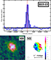 |
Fig. 6. Same as in Figure 5, but for B15-15. |
| In the text | |
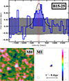 |
Fig. 7. Same as in Figure 5, but for B15-25. |
| In the text | |
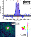 |
Fig. 8. Same as in Figure 5, but for B15-27. |
| In the text | |
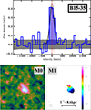 |
Fig. 9. Same as in Figure 5, but for B15-35. |
| In the text | |
|
Fig. 10. Same as in Figure 5, but for ALMA-114. We detect no emission towards the location of B15-114, but in the north-east towards a source labelled ALMA-114 in this work. The moment-0 map (centred on the new source detection) shows a significant detection (S/N ∼ 6) associated with a broad CO (2-1) line detection, very close in redshift to B15-114 (indicated with the vertical dotted line in the spectrum). The lower S/N feature in the south-west of the image is not associated with the B15-114 source, which is instead located 0.5″ south of it. |
| In the text | |
|
Fig. 11. Molecular gas-mass function derived from the observed group at zspec = 1.284 compared to works in the literature by (Decarli et al. 2019, 2020, D19 and D20, at 1.0 < z < 1.7), (Lenkić et al. 2020, L20, at 1.2 < z < 1.7), and (Messias et al. 2024, M24, at 1.0 < z < 1.8). The results by Berta et al. (2013, different line types for different redshift ranges) were derived from empirical scaling relations, instead of inferring MH2 from CO as the previously cited works. The empty boxes show the results from our study. These are 0.5 dex wide in molecular gas mass (centred at each step of 0.25 dex), and the vertical width shows the statistical uncertainty. |
| In the text | |
|
Fig. 12. Cosmic molecular gas-mass density in group environments derived using the group identified by MUSE and detected by ALMA in CO (2-1) at z = 1.284 (blue data point and error bar). For reference, literature estimates are also included. The CO-derived estimates reported by Decarli et al. (2020) from z = 0.271 to 4.475 appear as filled grey boxes, and those at 1 ≲ z ≲ 3 reported by Messias et al. (2024) appear as empty boxes. The sub-millimeter continuum derived trend from Scoville et al. (2017) is displayed as a continuous filled grey region. The cosmic mass density is plotted as the ratio to the critical cosmic density. |
| In the text | |
|
Fig. B.1. The natural-weighted 3mm continuum map with a 0.5” uv-taper (gray scale) with contours overlaid from the IRAC-3.6 μm map (red isocontour levels at 3, 6, and 12σ). Sources that revealed CO (2-1) line emission are marked with open blue stars, while the continuum detections reported in Table 4 are marked as blue circles. The potential 3σ continuum detection toward an IRAC source is marked with a blue square. |
| In the text | |
|
Fig. C.1. Comparison between HST WFPC2/F814W imaging (background gray image) and the CO (2-1) maps (red contours) for the detected sources. Cutouts are 4″ wide (∼34 kpc). The contours indicate levels at |
| In the text | |
Current usage metrics show cumulative count of Article Views (full-text article views including HTML views, PDF and ePub downloads, according to the available data) and Abstracts Views on Vision4Press platform.
Data correspond to usage on the plateform after 2015. The current usage metrics is available 48-96 hours after online publication and is updated daily on week days.
Initial download of the metrics may take a while.