| Issue |
A&A
Volume 706, February 2026
|
|
|---|---|---|
| Article Number | A339 | |
| Number of page(s) | 20 | |
| Section | Stellar structure and evolution | |
| DOI | https://doi.org/10.1051/0004-6361/202554004 | |
| Published online | 19 February 2026 | |
Physical interpretation of the oscillation spectrum on the red giant branch and the asymptotic giant branch
1
LIRA, Observatoire de Paris, Université PSL, Sorbonne Université, Université Paris Cité, CY Cergy Paris Université, CNRS 5 Place Jules Janssen 92190 Meudon, France
2
School of Physics, University of New South Wales Sydney NSW 2052, Australia
3
Univ. Rennes, CNRS, IPR (Institut de Physique de Rennes) – UMR 6251 F-35000 Rennes, France
4
Instytut Astronomiczny, Uniwersytet Wrocławski ul. Kopernika 11 51-622 Wroclaw, Poland
★ Corresponding author: This email address is being protected from spambots. You need JavaScript enabled to view it.
Received:
3
February
2025
Accepted:
22
September
2025
Abstract
Context. The high frequency resolution of the four-year time series collected by the space-borne telescope Kepler provides us the opportunity to study the seismic mode structure of highly luminous giants in great detail. Seismic observables can be used to infer the interior structure through comparisons with stellar models. However, we still need to extend the physical interpretation of previously observed seismic differences between hydrogen-shell burning (red giant branch; RGB) and helium-burning (red clump and asymptotic giant branch; AGB) stars towards high luminosity stages.
Aims. Here we aim to investigate which physical conditions differ between H-shell and He-burning stars in the helium-second ionisation zone, based on the signature this zone imprints on mode frequencies. In addition, we explore the sensitivity of seismic parameters to the physics implemented in the models.
Methods. We used a grid of stellar models with masses between 0.8 M⊙ and 2.5 M⊙ and metallicities between −1.0 dex and 0.25 dex. Transfer mechanisms such as mass loss, core, envelope overshooting, and thermohaline mixing were implemented. We inferred the p-mode frequencies of the models by artificially suppressing the gravity modes in the core.
Results. In accordance with observations, we find that the main stellar properties affecting the seismic observables in the models are the stellar mass and metallicity. Mass loss on the RGB and rotation-induced mixing from the main sequence to the early-AGB cause a phase difference in the helium ionisation zone glitch signature between H-shell and He-burning stars. The amplitude of the glitch signature in the local large separation, Δν, correlates with the density in the helium ionisation zone, which explains the different glitch amplitudes observed between the H-shell and He-burning stars. The amplitude exceeds 10% of the observed value of Δν in high-luminosity red giants, which makes the asymptotic expansion less accurate when Δν ≤ 0.5 μHz.
Conclusions. An efficient mass loss on the RGB, typically encountered when M ≤ 1.5 M⊙, can explain the classification of H-shell and He-burning stars based on the p-mode pattern. When M ≥ 1.5 M⊙, efficient mixing mechanisms might leave an important detectable signature in the p-mode frequencies, permitting a potential classification of these stars.
Key words: stars: AGB and post-AGB / stars: evolution / stars: interiors / stars: late-type / stars: low-mass / stars: oscillations
© The Authors 2026
 Open Access article, published by EDP Sciences, under the terms of the Creative Commons Attribution License (https://creativecommons.org/licenses/by/4.0), which permits unrestricted use, distribution, and reproduction in any medium, provided the original work is properly cited.
This article is published in open access under the Subscribe to Open model. This email address is being protected from spambots. You need JavaScript enabled to view it. to support open access publication.
1. Introduction
A breakthrough in our understanding of stellar structure and evolution has been provided by the advent of the space missions CoRoT (Baglin et al. 2006), Kepler (Borucki et al. 2010; Gilliland et al. 2010), K2 (Howell et al. 2014), and, more recently, TESS (Ricker et al. 2015). The ultra-high precision photometric data collected by these space-borne telescopes provide access to the frequencies of stellar oscillation modes. The observables describing the global frequency patterns of stars can be used to determine their masses, and hence mass loss, through the use of seismic scaling relations (Miglio et al. 2012, 2021; Kallinger et al. 2018; Yu et al. 2021). The more detailed fine structure of the frequency patterns can be used to estimate the evolutionary stage of red giant stars (Bedding et al. 2011; Kallinger et al. 2012; Vrard et al. 2016; Hon et al. 2017, 2018; Mosser et al. 2019). Mosser et al. (2011) have shown that the asymptotic p-mode frequencies ( ) of red giants, which are derived under the assumption that n ≫ ℓ, can be expressed as
![Mathematical equation: $$ \begin{aligned} \nu _{n,\ell }^{\mathrm{UP} } = \left(n + \frac{\ell }{2} + \varepsilon - d_{0\ell } + \frac{\alpha }{2}[n - n_{\rm max}]^{2}\right)\Delta \nu , \end{aligned} $$](/articles/aa/full_html/2026/02/aa54004-25/aa54004-25-eq2.gif) (1)
(1)
where UP stands for universal pattern, n is the mode radial order, ℓ is its degree, ε is the acoustic offset that allows us to locate the radial modes in the spectrum, and Δν is the observed mean frequency spacing between consecutive radial modes (the large frequency separation). Moreover, d0ℓ is a reduced small frequency separation defined as d0ℓ = δν0ℓ/Δν, where δν0ℓ is the small frequency separation between a mode of degree ℓ and its neighbouring radial mode. The curvature term, α = (dlogΔν/dn), accounts for the linear dependence of the large frequency separation on the radial order, and nmax = νmax/Δν − ε is the equivalent radial order that the frequency of the maximum oscillation power νmax would have.
The observed frequencies νn, ℓ are of major importance, as they are sensitive to the stellar internal structure (Tassoul 1980; Scherrer et al. 1983) and can be used to probe interior stellar physics such as overshooting (e.g. Baudin et al. 2012; Bossini et al. 2015; Khan et al. 2018; Dréau et al. 2022). Specifically in main-sequence stars, the small separations d0ℓ are sensitive to regions with strong gradients of sound speed (Gough 1986) and can be used to probe the stellar structure at localised depths (Roxburgh & Vorontsov 2003). Observations of giant stars have highlighted that these small separations depend on stellar mass (Huber et al. 2010). The resulting distribution of small separations d0ℓ at fixed Δν can be theoretically explained by a difference in the distance between the location of the bottom of the convective envelope and the inner turning point of the mode cavity for stars with different masses (Montalbán et al. 2010), especially for dipole modes (ℓ = 1).
It has been shown both observationally and theoretically that the frequency pattern of the acoustic modes changes as stars evolve up the red giant branch (RGB). The dipole modes move closer to their neighbouring radial mode, while the quadrupole modes move slightly away, resulting in a triplet, fork-like pattern in the frequency spectrum (Stello et al. 2014; Dréau et al. 2021). As this occurs, the observational range of modes also shifts to a narrower frequency range towards lower frequencies, resulting in fewer modes with lower radial orders (Mosser et al. 2013a; Trabucchi et al. 2017; Yu et al. 2020).
The so-called semi-regular variables, which are solar-like pulsators at high luminosity stages (Dziembowski et al. 2001; Christensen-Dalsgaard et al. 2001), exhibit only a small number of stochastically excited oscillation modes, limiting the power of seismology to probe their interiors. Moreover, the assumption that n ≫ ℓ is no longer satisfied, and hence the modes are no longer expected to follow the asymptotic pattern given by Eq. (1). Here, we explore the limits of the asymptotic approach and assess its potential to describe the oscillation spectrum of high-luminosity red giants.
As presented here, Eq. (1) assumes that the Jeffreys, Wentzel, Kramers and Brillouin (JWKB) approximation, which states that the physical parameters inside the star vary on a scale much greater than the wavelength of the oscillations, is valid. However, clear signatures of sharp structural variations were initially predicted (Vorontsov 1988), and subsequently confirmed for the Sun (Houdek & Gough 2007), for main-sequence stars (Lebreton & Goupil 2012; Mazumdar et al. 2012, 2014; Verma et al. 2014; Deheuvels et al. 2016), and for red giants (Miglio et al. 2010; Broomhall et al. 2014; Vrard et al. 2015; Corsaro et al. 2015). These structural variations are called glitches (Gough 2002) and are known to introduce a smooth frequency-dependent modulation to the otherwise regular asymptotic mode frequencies νn, ℓ given by Eq. (1) (Gough 1990). Three main structural variations have been identified, which are the base of the convective envelope, the helium ionisation zones, and the boundary of the convective core (Monteiro et al. 1994; Monteiro & Thompson 2005; Houdek & Gough 2007; Cunha & Metcalfe 2007; Deheuvels et al. 2016). In red giants, the helium second-ionisation (HeII) zone creates the dominant glitch (Miglio et al. 2010). The glitch signature is expected to depend on such stellar properties as helium abundance (Houdek & Gough 2007; Houdayer et al. 2021, 2022), which paves the way for estimating the helium abundance in cool stars (e.g. Vorontsov et al. 1992; Lopes et al. 1997; Broomhall et al. 2014; Verma et al. 2014, 2019; Farnir et al. 2019). Also, the study of the HeII zone signature in intermediate- and high-luminosity red giants has shown that the glitch morphology (such as the amplitude, phase, and frequency dependence of the glitch-induced frequency modulation) depends on the evolutionary stage (Vrard et al. 2015; Dréau et al. 2021). It is particularly interesting that the glitch modulation is stronger and phase-shifted during He-burning phases compared to the H-shell burning phase. This enables a classification between RGB and He-burning stars, including clump and asymptotic giant branch (AGB) stars. In the following, we aim to investigate the physical origin of these differences caused by stellar evolution, which are attributed to a change in the temperature and the density in the HeII ionisation zone (Christensen-Dalsgaard et al. 2014).
In this work, we focus on the oscillation spectra of evolved red giants. By means of the Aarhus adiabatic oscillation package (ADIPLS, Christensen-Dalsgaard 2008), we extract the p-mode frequencies of stellar models derived with the evolution code Modules for Experiments in Stellar Astrophysics (MESA, Paxton et al. 2011, 2013, 2015, 2018, 2019). We investigate the impact of input physics on seismic parameters in comparison with observations. We analyse the physical differences between RGB and AGB stars deduced from their different glitch signatures and explore the limits of the asymptotic expansion (Eq. 1) at stages of high-luminosity. In Sect. 2, we describe the set of input physics applied in our MESA calculations. The procedure used to extract the p-mode pattern of evolved red giants, including RGB and clump and AGB stars, is described in Sect. 3. We examine how the seismic parameters vary as a function of both the evolutionary stage and stellar parameters in Sect. 4. Then, we discuss the validity of the asymptotic expansion and the differences in the oscillation spectrum between RGB and AGB stars in Sect. 5. Finally, we conclude in Sect. 6.
2. Stellar models
A grid of stellar models with initial mass M = [0.8, 0.9, 1.0, 1.1, 1.2, 1.5, 1.75, 2.0, 2.5] M⊙, initial metallicity [Fe/H] = [ − 1.0, − 0.5, − 0.25, 0.0, 0.25] dex, and different input physics has been computed with the release 12778 of the stellar evolution code Modules for Experiments in Stellar Astrophysics (MESA, Paxton et al. 2011, 2013, 2015, 2018, 2019). Modelling is exhaustively described in Dréau et al. (2022). Here, we summarise the main input physics that are likely to affect seismic observables. We used the 1M_pre_ms_to_wd1 test suite case and defined a reference model from which the input physics are modified (Table 1). Convection was treated following the mixing-length theory formalism, where the convective efficiency was taken to vary with the opacity of the convective element, especially in the outer stellar layers (Henyey et al. 1965). Three sets of opacity tables were used to take the changing internal temperature and chemical composition into account. At low temperature (log T < 3.95), we used the AESOPUS tables (Marigo & Aringer 2009), which allowed us to account for such continuum and discrete sources as molecular absorption bands and collision-induced absorption in the photosphere of AGB stars. At high temperatures (log T > 4.05), we took OPAL1 (Opacity Project At Livermore) tables for regions that do not experience metal enrichment, applicable before He burning, and OPAL2 tables for those that undergo C and O enhancements due to He burning (Iglesias & Rogers 1996). The transition from one opacity table to another was treated as explained in Paxton et al. (2011). According to their Eq. (1), AESOPUS and OPAL1 tables are blended in the interval log T = 4.00 ± 0.05, while the transition from OPAL1 to OPAL2 was carried out in the region where the metal mass fraction increased by an amount dZ, dZ ∈ [0.001, 0.01].
Specifications of the MESA reference stellar model
Mixing processes in stellar interiors affect the chemical composition profile and the physical evolution of layers near the boundary of convective zones. Mixing therefore has non-negligible effects on the stellar oscillation modes that probe these layers. For instance, extending the mixing beyond the convective core instability boundary defined by the Schwarzschild criterion significantly modifies the period spacing ΔΠ1 of dipole modes (Bossini et al. 2015). Here, we considered several mixing processes in both the core and the envelope. Among these, we took convective core overshooting and envelope undershooting into account to extend the mixing beyond the Schwarzschild boundary (above the core and below the envelope). In MESA, we assumed that the temperature gradient ∇T is equal to the radiative gradient ∇rad in the extra mixing region (Zahn 1991), and we followed a step scheme (e.g. Maeder 1975), in which the additional mixing region spreads over a distance
 (2)
(2)
where HP is the pressure scale height at the boundary of the convective zone and Rcz is the radial thickness of the convective zone. In particular, we applied core overshooting during core nuclear burning phases, where a convective core grows with time. Including overshooting modifies the radiative gradient ∇rad profile in the extra mixing region through an opacity increase. This may bring ∇rad above ∇ad, then leave the boundary of the convective core ambiguous (Bossini et al. 2017). To avoid misidentifying the convective border in MESA, we followed the treatment presented in Bossini et al. (2017), which defines the convective border either at the position of the local minimum of ∇rad if it increases over ∇ad in the extra mixing region, or otherwise at the usual border of convective instability where ∇rad = ∇ad. We also included envelope undershooting from the main sequence up to the AGB following Khan et al. (2019). When He-core overshooting was applied, we included a partially mixed He-semi-convection region between the convective core border and the outer radiative zone, according to the diffusion scheme presented in Langer et al. (1985) where the efficiency factor αsc is 0.1.
Once the hydrogen-burning shell reaches the homogeneous zone of the envelope after the first dredge-up, nuclear reactions in the shell, such as 3He(3He, 2p)4He, create an inversion of molecular weight (Ulrich 1972; Eggleton et al. 2006, 2008; Charbonnel & Zahn 2007). Thermohaline convection sets in when the molecular weight gradient becomes negative (i.e. ∇μ = dlnμ/dlnP < 0) in regions that are stable against convection (according to the Ledoux criterion). As a result, this mixing process occurs between the convective envelope and the H-burning shell surrounding the degenerate core and affects the surface composition, especially for stars of mass below 1.5 M⊙ (Cantiello & Langer 2010; Lagarde et al. 2012). In MESA, we treat thermohaline convection as a diffusive process (Kippenhahn et al. 1980), taking the diffusion coefficient presented in Sect. 4.2 of Paxton et al. (2013) with the efficiency parameter αth = 2 when effective. In our models, we did not include such microscopic diffusion as atomic diffusion and radiative acceleration. Although this process has been shown to be non-negligible around the hydrogen-burning shell, significantly affecting the location of the RGB bump, it only weakly alters the helium core mass at the helium flash (Michaud et al. 2010). As an additional test, we applied the atomic diffusion settings of the 1.5M_with_diffusion2 test case to the reference model listed in Table 1, from the main sequence to the luminosity tip of the RGB, and found that they had a negligible impact on the seismic parameters described in Eq. (1), as measured on the RGB.
Finally, we considered a simple grey atmosphere with an Eddington T(τ)-law, where τ is the optical depth. In MESA, the interior is connected to the atmosphere at the meshpoint corresponding to τ = 2/3, which lies at the photospheric boundary where T = Teff (Paxton et al. 2011). At high luminosity stages, stars experience significant mass loss due to the radiative pressure pushing the envelope outwards. On the RGB, we used Reimers’s prescription (1975), which reads
 (3)
(3)
while on the AGB, we adopted Blöcker’s prescription (1995):
 (4)
(4)
In the previous equations, the scaling factors are ηR = 0.3, which is the maximum mass loss rate reported among several stellar-cluster populations with different age and chemical compositions (Miglio et al. 2021), and ηB = 0.1, which allows us to reproduce both the initial-final mass relation across evolution and the AGB luminosity function (Choi et al. 2016).
The mode frequencies associated with the MESA models were computed using the stellar oscillation code ADIPLS (Christensen-Dalsgaard 2008). In the ADIPLS settings, we did not consider the Cowling approximation and solved the full set of fourth-order system of oscillation equations. The first trial frequency was considered low enough to find the first radial order, after which the next trial frequencies were taken just above the mode frequencies computed at the previous radial order. The differential equations were integrated following the shooting method with centred difference equations, where the differential equations were replaced by difference equations. In this case, the solutions were integrated separately from the inner and outer boundaries while satisfying the boundary conditions. In addition, the eigenvalue connected to the frequency was determined by matching these solutions at the specific point r/R = 0.5, where R is the stellar radius. If the frequency was below the acoustic cut-off frequency, the surface boundary condition was imposed by matching the interior solution to the exponentially decaying form that arises in an isothermal atmosphere at the matching point. We emphasise that the isothermal atmosphere was applied only for the boundary condition in the mode frequency calculations; in the MESA structure models, the atmosphere is not isothermal. For higher frequencies, the surface pressure boundary condition is instead given by δp = 0, where δp is the Lagrangian perturbation in pressure. Subsequently, the computed frequencies were improved by using the Richardson extrapolation, which allowed us to reduce the numerical errors due to the finite number of meshpoints (Shibahashi & Osaki 1981).
3. P-mode pattern extraction
3.1. Computing the model pressure mode frequencies
In red giants, the p- and g-mode cavities are coupled (Bedding et al. 2011). As a consequence, non-radial modes are mixed, behaving as p modes in the envelope and g-modes in the core. As a result of the coupling, mixed mode frequencies deviate from the expected pure p-mode (and pure g-mode) frequencies. The observed mixed modes with the largest amplitudes are those with the lowest inertia, as they need less energy input to be excited to observable amplitudes. These modes are also the most p-like, meaning that their frequencies are the closest to the acoustic resonances of the envelope (the frequencies that pure p-modes would have in the absence of the core). For evolved giants with νmax ≤ 40 μHz, or equivalently Δν ⪅ 4 μHz, it has been shown that the frequency of the mixed mode of lowest inertia, near each acoustic resonance, could be used as an approximate estimate for the frequency of the acoustic resonance (Broomhall et al. 2014). However, the computations required us to first find this mode and to obtain an accurate estimate of its frequency makes this a time-consuming approach. To address this difficulty, we followed an approach inspired by Ball et al. (2018), who set the squared Brunt–Väisälä frequency  to zero in non-convective regions (i.e. where
  ). In this scenario, the cavity of g modes was removed, and hence we had no mixed modes, just pure p modes. This method is efficient for extracting the p-mode frequencies of dipole and quadrupole modes in RGB models with Δν ≤ 4.5 μHz, showing a difference within 0.02Δν relative to the frequencies of the lowest inertia modes (Ball et al. 2018). While our treatment is based on the same principle, it differs in its implementation. In their analysis, Ball et al. (2018) defined an artificial Γ1 (their Eq. 1) to maintain consistency within the oscillation equations. In our implementation, we retained the original Γ1 profile. This choice has a negligible effect on the quadrupole mode frequencies but introduces a bias of 0.01Δν in the dipole mode frequencies at low Δν (Δν ≤ 4.5 μHz). The magnitude of this bias is comparable to the precision with which the pressure-mode frequencies were extracted in Ball et al. (2018). This bias has only a limited effect on the glitch signature in the large frequency separation, which is computed from the difference between consecutive radial orders at fixed degree. In this case, the bias is largely mitigated. The parameter most sensitive to this effect is the reduced small separation d01 between dipole (ℓ = 1) and radial (ℓ = 0) modes. Nevertheless, we show in Sect. 4.2 that our interpretations are not affected by the presence of this bias. Similarly, we examine the applicability of this method for clump and AGB stars in the following section.
Finally, we performed a mesh redistribution to optimise the computation of p modes. This step was necessary as ADIPLS would have otherwise failed to compute the mode parameters at low-radial orders. This is particularly important for high-luminosity stages because the maximum oscillation power is located at low radial order (Mosser et al. 2013a; Stello et al. 2014; Yu et al. 2020). To further ensure we did not miss any non-radial modes, we ran ADIPLS with a variety of mesh redistributions. This mesh redistribution also guarantees the displacement eigenfunctions are resolved, regardless of the evolutionary status. Our analysis rests on a fixed number of modes, associated with the seven radial orders that are the closest to νmax, estimated by the scaling relation
 (5)
(5)
where νmax, ⊙ = 3050 μHz, Δν⊙ = 135.5 μHz and Teff, ⊙ = 5780 K (Kjeldsen & Bedding 1995; Mosser et al. 2013b). This number of modes is representative of the number of observed modes for the least evolved stars in our sample (near Δν ∼ 4 μHz) but in excess relative to the most luminous RGB and AGB stars. We chose a fixed number of modes to ensure the consistency of the determination of the glitch signature.
3.2. Validating the computation of pressure modes
To check if our method for calculating the pure p-modes would yield satisfactory results, we compared their frequencies with those of the mixed modes with the lowest inertias. The comparison was done for our reference models in the He-burning phase defined in Table 1. We used a fixed number of about 20 000 mesh points for this, as it was sufficient to resolve the eigenfunctions of the mixed modes and thereby reliably extract their frequencies. We obtained a set of several mixed modes per radial order n, or equivalently per Δν interval. We took the frequencies of the modes of lowest inertia per radial order n as a reference for the expected pure p-mode frequencies. For each reference, we derived the difference to the pure p-mode frequency (the one derived by setting  ). The results are shown in Figs. 1a and c. Because most of the frequency differences are within 0.05 Δν (b and d panels), we conclude that the pure p-mode frequencies are precise representations of the acoustic resonances of the envelope. However, for the dipole modes we do notice a mean difference of ∼0.02Δν between the two ways of estimating the acoustic resonant frequencies (see vertical solid line in panel b). This bias has limited consequences for the study of the glitch signature because the signature is extracted from the large frequency separation Δνn, ℓ (Eq. 9), which is defined as the difference in frequencies at consecutive radial order n at the same degree ℓ (Eq. 8). However, the spread of ∼0.05 Δν, may impact the amplitude of the glitch modulation, which is typically lower than Δν/10. In Sect. 4, we show that these differences do not prevent us from accurately reproducing the shape of the modulation. Quadrupole modes are better derived compared to dipole modes, with an unbiased measurement of their frequencies. In fact, the inner turning point of the dipole p-mode cavity is located deeper within the interior than that of the quadrupole p-mode cavity, resulting in stronger coupling with the g-mode cavity where
  , hence producing a more pronounced deviation in the dipole mode frequencies.
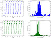 |
Fig. 1. Comparison of the mode frequencies computed using the method |


The reason for the above frequency differences could be one of the following. First, some mixed modes are poorly estimated because the ADIPLS settings we chose were not optimised for any Δν. For instance, mesh redistribution could be improved at low Δν ≤ 1 μHz to better resolve the displacement eigenfunctions of mixed modes. Second, although the modes of lowest inertia are the mixed modes closest to the expected pure pressure modes, they still deviate a bit from the latter. To estimate this deviation, we fitted a Gaussian profile to the mode inertia profiles within each Δν interval, thereby locating the acoustic resonance, and find that its difference from the mode of lowest inertia averages 0.01Δν. Finally, by keeping the inconsistent Γ1 profile as presented in Sect. 3.1, a bias of approximately 0.01Δν is introduced in the dipole mode frequencies at low Δν (Δν ≤ 4.5 μHz).
The errors introduced in the dipole and quadrupole mode frequencies by setting  while retaining inconsistent Γ1 profiles in the core (see Figs. 1b and d) are, on average, of the same order of the largest errors reported by Ball et al. (2018), who applied the same technique to RGB models but with consistent Γ1 profiles. In the following, we use the dipole and quadrupole mode frequencies obtained by setting
  in the core without changing the Γ1 profiles as the reference frequencies for the pure pressure dipole and quadrupole modes, for both RGB and clump and AGB stars. In parallel, we compute the radial modes with the unmodified MESA models. These radial, dipole, and quadrupole modes constitute the set of modes used in our study.
3.3. Deriving the seismic parameters
In this work, we aim to interpret the observational results of Dréau et al. (2021) in terms of internal structure differences between RGB and AGB stars. With the set of frequencies described in Sect. 3.1, we computed the seismic parameters corresponding to the acoustic offset (ε) and the reduced small frequency separation (d0ℓ). The large frequency separation, Δν, was taken as the slope of the unweighted linear fit to the radial-mode frequencies versus their radial order n.
The local acoustic offset ε(n), which represents the frequency spacing at radial order n between the radial mode at frequency νn, 0 and nΔν, was computed as
 (6)
(6)
The dimensionless local small frequency separations d0ℓ(n) in fraction of Δν were defined as
![Mathematical equation: $$ \begin{aligned} \left\{ \begin{array}{ll} d_{01}(n) = \frac{1}{2\Delta \nu }\left(\nu _{n,0} - 2 \ \nu _{n,1} + \nu _{n+1,0}\right) \\ [4pt] d_{02}(n) = \frac{\nu _{n, 0} - \nu _{n-1, 2}}{\Delta \nu }, \end{array} \right. \end{aligned} $$](/articles/aa/full_html/2026/02/aa54004-25/aa54004-25-eq17.gif) (7)
(7)
and the global seismic parameters ε and d0ℓ were taken as the average of the local values computed with our set of frequencies while the uncertainties were obtained as the standard deviation of the local values.
The method we used to extract the glitch parameters is in many aspects similar to that adopted in Dréau et al. (2021). We inferred the glitch signature  by evaluating the difference between the measured local large frequency separation Δνn, ℓ defined by
 (8)
(8)
and the expected value  without glitch derived from Eq. (1), which gives
 (9)
(9)
where  . We then fitted the glitch signature by a damped oscillator function
 (10)
(10)
where 𝒜gl and 𝒢gl are, respectively, the dimensionless amplitude and period of the glitch modulation in units of Δν. Φgl is the phase of the modulation centred on νmax (Vrard et al. 2015). The uncertainties of the glitch parameters were extracted from the covariance matrix resulting from the Levenberg-Marquardt algorithm to fit the glitch signature. The main difference between this method and that adopted in Dréau et al. (2021) lies in the choice of the initial guess for the glitch period 𝒢gl. The range of all possible values taken by the glitch parameters is large throughout the evolution from the RGB up to the AGB, and the optimisation function to be minimised has several local extrema according to the modulation period 𝒢gl. This complication is even more relevant at low Δν because there the asymptotic expansion (Eq. 1) is less accurate, which makes it hard to extract the glitch signature. In order to mitigate the bias induced by the choice of initial conditions, the optimised glitch parameters of one stellar model were given as initial guesses for the glitch parameters at the next model. This allowed us to extract glitch parameters that smoothly evolve between consecutive stellar models.
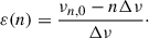
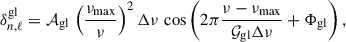
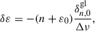
Finally, we investigated the correlations between the physical properties of the HeII ionisation zone and the glitch parameters. As illustrated in Fig. 2, we characterise the HeII ionisation zone by three parameters. These are the amplitude, HHeII, of the associated dip in the first adiabatic exponent Γ1, the acoustic radius, tHeII, of the dip (meaning the time for a sound wave to travel from the stellar centre to that location), and the width, bHeII, of the dip. Hereafter, both tHeII and bHeII are normalised by the total acoustic radius of the star T0 = 1/(2Δνas), which is the total time it takes a sound wave to travel from the centre to the surface. Here, Δνas is the asymptotic large frequency separation:
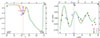 |
Fig. 2. (a) Profile of the first adiabatic exponent Γ1 as a function of the normalised acoustic radius in a 1 M⊙ RGB model computed with MESA at Δν = 1.65 μHz. The parameters of the Γ1 variations (HHeII, tHeII, and bHeII) are directly shown in the figure. The solid green line is the Γ1 profile throughout the star. The thick dashed orange line indicates the baseline that connects the local maximum after the dip caused by the second He-ionisation with the Γ1 profile before the dip. The thin dashed red line gives the fit of the Γ1 profile with Eq. (12) around the dip. (b) Glitch modulation induced by the second He-ionisation zone in the same model, as in the left panel. The local large separation Δνn, ℓ is shown in red circles, blue triangles, and green squares for radial, dipole, and quadrupole modes, respectively. The solid green line is the damped oscillator model given by Eq. (10) fitted to the data points. We point out that the data points are plotted at the mean frequencies (νn, ℓ + νn + 1, ℓ)/2. The upper x-axis indicates the radial order of ℓ = 0 modes, and the dotted blue line locates the maximum oscillation power. |
 (11)
(11)
where cs is the sound speed. We fit the Γ1 profile in the vicinity of the dip by a Gaussian on top of a linear baseline as follows:
 (12)
(12)
where t is the normalised acoustic radius, a0 and a1 are the coefficients of the linear baseline of the Γ1 profile (dashed orange line). In the fitting process, HHeII, tHeII, and bHeII are left as free parameters, but a0 and a1 are fixed by connecting the local maximum below and above the Γ1 dip.
4. Seismic diagnostics for RGB and AGB stages
In Dréau et al. (2021), we were able to accurately extract the seismic parameters of stars with Δν values down to 0.5 μHz with the 1470-day time series of Kepler. Hereafter, we examine the p-mode parameters obtained with ADIPLS, giving us the opportunity to compare the seismic parameters derived from observations to those from stellar models, as well as to extend the analysis up to higher luminosity stages of the RGB and AGB (equivalent to Δν ≳ 0.06 μHz).
4.1. Oscillation spectrum across evolution
Following the representation by Stello et al. (2014), we show in Fig. 3 the structure of the oscillation spectrum at different evolutionary stages with each row displaying the frequencies of one model. From the top, they span from νmax ∼ 40 μHz (or Δν ∼ 4 μHz, equivalent to red clump luminosities) to more luminous stars with νmax ∼ 0.1 μHz (or Δν ∼ 0.06 μHz). RGB (panel a) and clump plus AGB (panel b) stages are shown separately. As reported in Stello et al. (2014), the dipole modes are no longer located roughly halfway between adjacent radial modes as predicted by the asymptotic pattern (Tassoul 1980). Rather, they get closer to the right-hand side radial and quadrupole modes, forming a triplet pattern. This behaviour is even more pronounced at low radial orders, which are detectable for low Δν stars (as indicated by the modes between the dashed magenta lines). In addition, the whole oscillation spectrum narrows when Δν decreases. This explains why the observed frequency spacings between non-radial modes and the neighbouring radial mode narrows as stars become more luminous, as described in previous studies (e.g. Bedding et al. 2010; Mosser et al. 2011; Huber et al. 2011; Yu et al. 2020; Dréau et al. 2021). No clear difference can be seen between the radial and non-radial mode patterns of RGB and clump and AGB stars, except that the spacing between radial and non-radial modes differs slightly at fixed Δν (Montalbán et al. 2010, 2012).
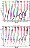 |
Fig. 3. Model frequencies from radial order n = 1 up to n = 8 computed with ADIPLS for a 1 M⊙ track at solar metallicity. The MESA models are computed with the reference input physics listed in Table 1. Radial, dipole, and quadrupole modes are shown in red circles, blue triangles, and green squares, respectively. For the RGB (panel a), the grey frequencies are clump plus AGB models for comparison, and vice versa for the clump plus AGB (panel b). The non-radial modes (ℓ = 1, 2) are computed by setting the squared Brunt–Väisälä frequency |


When νmax ≲ 10 μHz, we see that the radial and non-radial ridges significantly deviate from vertical ridges, which we would not expect if the modes follow the asymptotic relation. The asymptotic relation assumes that physical properties vary smoothly in the interior. These assumptions may not be valid any more at high-luminosity stages, in particular because of the occurrence of such sharp structural variations as the HeII ionisation zone that are not taken into account in the asymptotic expansion. This would explain the significant departure from the asymptotic ridges. The validity of the asymptotic approach is discussed in further details in Sect. 5. Finally, we note the presence of non-radial modes with frequencies below that of the fundamental radial mode. As discussed in Stello et al. (2014), these could be related to f modes (Cowling 1941; Unno et al. 1989). F-modes are suspected to produce the sequence F near the fundamental sequence C in the period-luminosity diagram of semi-regular variable stars (Stello et al. 2014).
4.2. Seismic parameters in the asymptotic relation
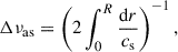
The dependence of the acoustic offset ε and the dimensionless small separations d0ℓ on stellar evolution is shown in Fig. 4. In agreement with White et al. (2011), we see in Fig. 4a that ε decreases as RGB stars become more luminous (blue line). Here we show AGB stars follow a similar trend (red line). However, the differences seen between the RGB and clump plus AGB stars visible for Δν ≳ 0.3 μHz are caused by the signature of the HeII ionisation zone. When computing ε with Eq. (6), this signature is ‘absorbed by’ the ε term and tends to vanish when averaged over a large number of modes. As proposed by Kallinger et al. (2012), this local signature in ε allows us to perform an efficient classification between RGB, clump and AGB stars based on the values of ε and Δν.
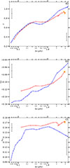 |
Fig. 4. Synthetic seismic parameters extracted from the p-mode frequencies computed with ADIPLS, as described in Sect. 3.3. The MESA models are computed with the reference input physics listed in Table 1, with M = 1.0 M⊙ and solar metallicity. (a) Variation of the acoustic offset ε as a function of Δν, with an emphasis on the evolutionary stage. Clump stars are shown by the orange ‘C’ symbols while the RGB and AGB are colour-coded in blue and red, respectively. ‘C’ symbols show the progress in the clump stage. Small (large, respectively), symbols correspond to the early (late, respectively), clump phase. The arrows indicate the direction of evolution. (b) and (c) Dimensionless small separations d0ℓ as a function of Δν. Mean error bars estimated for Δν below or above 0.5 μHz are represented on each panel. |
Figures 4b and 4c show that on both the RGB and AGB, d01 increases in absolute value (ℓ = 1 modes move closer to their higher-frequency radial mode neighbour) as Δν decreases. In parallel, d02 smoothly varies when Δν ∈ [0.2, 4.0] μHz and decreases when Δν ≤ 0.2 μHz on the RGB (ℓ = 2 also moves towards the radial mode). This behaviour agrees with the observations of evolved stars (Mosser et al. 2013a; Stello et al. 2014; Yu et al. 2020; Dréau et al. 2021). No clear distinction can be made in the d01 profile between RGB and clump and AGB models for M = 1.0 M⊙ as plotted here. However, we note that clump and AGB tend to have larger |d01| than RGB stars for M ≥ 1.5 M⊙. In Fig. 4b, we also note the uncertainties on d01, which reflect the dispersion of its values across the seven radial orders closest to the order of maximum oscillation power. These uncertainties are about 0.01 for Δν ≤ 0.5 μHz and 0.015 for Δν ≥ 0.5 μHz, i.e. of the same order of magnitude as the bias presented in Sect. 3.1 by keeping an inconsistent Γ1 profile while setting  in the radiative core. This confirms that our interpretations are not affected by this bias.
However, we do see a clear difference in d02 between RGB and clump plus AGB stars (Fig. 4c). In addition, we notice that the values of d01 and d02 are highly sensitive to the stellar mass and, to a lesser extent, to the mass-loss rate, as already presented in Huber et al. (2010), Montalbán et al. (2012), Dréau et al. (2021) and depicted in panels c, d, e, and f of Figs. B.1. These differences between RGB and clump plus AGB stars could be attributed to structure changes rather than mass loss processes, because the differences are also visible at high mass (M ≥ 1.5 M⊙), where the mass loss rate is smaller. These structure changes could involve the distance between the base of the convective zone and the location of the turning point of the non-radial mode cavities (Montalbán et al. 2010). Aside from the initial stellar mass that is the main parameter affecting the seismic parameters, the metallicity is also expected to impact the measurement of these seismic parameters. These changes can exceed 10% of the d02 values, but remain ∼5% of the ε and d01 values when switching [Fe/H] from 0 dex to −1 dex (see Fig. B.1). This could explain why we did not detect any clear metallicity effects in the sample of Kepler targets studied in Dréau et al. (2021), with metallicities from −0.75 dex to 0.25 dex.
4.3. Signature of the HeII ionisation zone
4.3.1. The glitch amplitude 𝒜gl
The evolution of the modulation amplitude of the glitch signature is shown in Fig. 5a. We notice that the amplitude is larger on the clump stage and AGB than on the RGB, by 40% on average. These results support the observations made for red giants (Vrard et al. 2015; Dréau et al. 2021). This difference between RGB and red clump plus AGB can be attributed to the strength of the Γ1 variation at the HeII zone. The depth HHeII of the Γ1 dip is larger in the clump and AGB phase than on the RGB (Fig. 5c), which demonstrates that the signature of the HeII zone on mode frequencies is stronger once He burning occurs. The physical origin of this difference is discussed in Sect. 5.
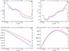 |
Fig. 5. Synthetic glitch and structure parameters computed with MESA and ADIPLS. The MESA models are the same as those shown in Fig. 4. The glitch amplitude 𝒜gl and period 𝒢gl are shown on the (a) and (b) panels, respectively, while the amplitude HHeII and the width bHeII of the HeII zone in the Γ1 profile are exhibited on the (c) and (d) panels, respectively. The label matches that of Fig. 4. In panel b, the additional solid light grey line is the modulation period expected from the location of the HeII ionisation zone tHeII, which is computed according to Eq. (13). |
4.3.2. The glitch period 𝒢gl
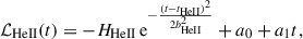
The glitch period is directly related to the HeII ionisation location by3
 (13)
(13)
where tHeII is the acoustic radius of the HeII ionisation zone normalised by the total acoustic radius of the stellar cavity T0 = 1/(2Δν). In Fig. 5b, we superimpose the modulation period inferred from Eq. (13) (grey curve) with that deduced from fitting the glitch modulation induced in the local large separation given by Eq. (10) (blue and red curves). We obtain identical values with each method, which confirms that the glitch signature is properly extracted. The modulation period computed from the mode frequencies decreases as Δν decreases, reflecting that the effective temperature – and consequently the internal temperature – also decreases as stars evolve along the RGB and AGB, causing the HeII ionisation zone to move closer to the centre. The decrease is in agreement with results from Kepler high-luminosity stars (Dréau et al. 2021), but we do find the trend to be steeper and the period values to be smaller in models than in Kepler data (compare the values and variations from the models in Fig. 5b with the median values shown in Appendix A).
In the following, we investigate the mass dependence of the glitch period 𝒢gl. As a supplementary study of the Kepler data analysis done in Dréau et al. (2021), in Appendix A we discuss in further detail the dependence of the modulation period on the stellar mass obtained with the sample of Kepler evolved stars used in Dréau et al. (2021). We notice that low-mass stars have a shorter modulation period than their high-mass counterparts at similar Δν, which is confirmed by stellar models (Fig. 6a). In parallel, in Fig. 6b, we see that regardless of mass, the period is the same at fixed effective temperatures. Such a behaviour is also found in the acoustic radius of the HeII zone (not shown). The difference in the modulation period (hence in the acoustic radius of the HeII zone) between low- and high-mass stars can be explained by a difference in effective temperature Teff, which is higher for high-mass stars at fixed Δν.
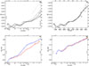 |
Fig. 6. Synthetic glitch period 𝒢gl and phase Φgl computed with ADIPLS. The MESA models are computed with the reference input physics listed in Table 1. (a) Dependence of the modulation period 𝒢gl on the stellar mass as a function of Δν during the RGB. The mass in solar units is shown with different shades of grey. (b) Same as (a), but for 𝒢gl as a function of Teff. (c) Evolution of the modulation phase Φgl with Δν for models of initial mass 0.9 M⊙ at solar metallicity, with an emphasis on the evolutionary stage. The labelling is identical to that in Fig. 4. (d) Same as (c), but for models of initial mass 1.5 M⊙. |
4.3.3. The glitch phase Φgl
In Kepler observations, RGB and clump plus AGB stars present a clear difference in the modulation phase, Φgl, of the glitch signature (Vrard et al. 2015; Dréau et al. 2021). This is also what we observe from the frequencies of the model with mass 0.9 M⊙ shown in Fig. 6c. There is a phase difference between clump plus AGB and RGB stars of about 1 radian all along the clump phase and the AGB, which results in a difference in the glitch contribution to Δν (Eq. 10). As shown in Sect. 4.2, differences in the measurements of the acoustic offset ε can be observed between AGB and RGB stars. These differences would be even more pronounced if the ε values were not averaged over several radial orders. They are in fact equivalent to those seen in the modulation phase Φgl. Differentiating Eq. (1) at fixed frequency highlights the connection between the small perturbations in ε and Δν, the latter being associated with the term  (Vrard et al. 2015):
 (14)
(14)
where δε is the contribution of the glitch signature to ε and ε0 is the acoustic offset in the absence of the glitch. This supports the observational results, showing that the physical basis, on which the classification of RGB and clump and AGB stars relies, is connected to the helium-second ionisation zone (Kallinger et al. 2012; Christensen-Dalsgaard et al. 2014; Vrard et al. 2015; Dréau et al. 2021).
Below, we investigate how the modulation phase difference between the RGB and red clump (RC) plus AGB depends on stellar mass. Figure 6d shows that, for a 1.5 M⊙ track, Φgl behaves very similarly for the two stages of evolution. This is in contrast to the reported phase difference from Kepler observations at all masses (see the lower-right panel of Fig. 4 of Dréau et al. 2021). We discuss this further in Sect. 5.
4.4. Influence of stellar model input physics on seismic parameters
In order to investigate the sensitivity of seismic parameters of the asymptotic pattern (Eq. 1) and the glitch signature (Eq. 10) with respect to input physics, we modified the parameters of the reference model (Table 1) step by step. The full scheme is detailed in Appendix B, and the relative differences between the reference model and the modified models are shown in Figs. B.1, B.2, and B.3. To summarise, the major parameters that strongly affect the seismic parameters are the stellar mass M and metallicity [Fe/H]. The initial helium abundance Y0 also significantly impacts the glitch parameters but does not alter the parameters of the asymptotic relation much. The mixing-length parameter αMLT and mass loss ηR mainly influence the modulation phase Φgl and the acoustic offset ε. Finally, the inclusion of extra-mixing regions, such as core overshooting, envelope undershooting, and thermohaline mixing, slightly affects the glitch parameters, while the impact on the seismic parameters from the asymptotic relation remains negligible. In Appendix B, we examine the effects of core overshooting during the main sequence for a 1 M⊙ model, where they are expected to be negligible due to the small convective core. For comparison, the impact of such overshooting on the modulation phase Φgl is discussed in Sect. 5.2 for a 1.75 M⊙ model, where the core convective zone is sufficiently developed to produce qualitatively noticeable effects.
5. Discussion
5.1. Understanding the strength of the glitch signal
The difference in the strength of the glitch signal reported in Sect. 4.3.1 between He-burning and H-shell burning phases reflects a difference in physical conditions and degree of ionisation in the envelope. The steeper the Γ1 variation, the stronger the glitch signature. As illustrated in Figs. 7a+c, we observe a clear dependence of the amplitude of the Γ1 variation, denoted HHeII, on the average temperature THeII and density ρHeII in the HeII ionisation region. Across all evolutionary stages considered, HHeII exhibits an approximately linear dependence on both log THeII and ρHeII. This trend is consistent with theoretical predictions indicating a steeper Γ1 profile in the HeII zone during the core He-burning phase (Christensen-Dalsgaard et al. 2014). Such a steepening results from the lower temperature and density in the convective envelope, reflecting the reduced envelope mass in AGB stars at a given value of Δν.
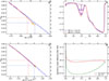 |
Fig. 7. (a) Dependence of the amplitude HHeII on the average temperature log THeII in the HeII zone. The input physics and label are the same as in Fig. 5 for models of mass 1 M⊙ and solar metallicity. Dotted lines show the log THeII − HHeII coordinates of the RGB and AGB models presented in the right panel. (b) Γ1 profiles on the RGB and AGB roughly at a similar Δν = 1.03 μHz. The arrows indicate the amplitude and the width of the Γ1 variation at the helium-second ionisation zone, in blue on the RGB and red on the AGB. (c) Same as panel a, but with the average density log ρHeII in the HeII zone instead of log THeII. (d) Logarithmic differences between the AGB and RGB models shown in (b) of the temperature (dot-dashed red line) and density (dashed green line) as a function of the normalised acoustic radius. The vertical solid and dashed lines indicate the location of the base of the convective envelope in the RGB and AGB models, respectively. |
Christensen-Dalsgaard et al. (2014) further emphasised that differences in envelope density, rather than temperature, primarily account for the observed discrepancies in Γ1 between RGB and clump stars. A similar inference can be drawn from our comparison of RGB and AGB models. In Fig. 7d, we find that for models with Δν ≈ 1 μHz, the density contrast throughout the convective envelope below the surface is more significant than the corresponding temperature difference. This enhanced density contrast affects the degree of helium ionisation and thus modifies the Γ1 profile accordingly.
5.2. Exploring the phase difference between RGB and clump or AGB stars
Mass loss can contribute to the phase difference in the glitch modulation between RGB and clump plus AGB stars highlighted in Sect. 4.3.3 at low mass. For instance, taking a lower mass-loss rate ηR from 0.3 to 0.1 (equivalent to a RC mass in the range [0.85 M⊙, 0.95 M⊙] for an initial mass of 1 M⊙) introduces an average phase shift between the modified and reference models ΔΦgl = Φgl, ηR = 0.1 − Φgl, ηR = 0.3 of 0.3 rad on the clump stage and AGB (see Fig. B.2f). As a consequence, the absence of mass loss reduces the difference between the modulation phase of RGB and clump plus AGB stars, which makes mass loss a solid candidate to explain this difference in low-mass stars. This would also explain why we do not notice any difference between RGB and clump and AGB stars in high-mass models with the same set of input physics because for those the mass loss is small, leading to similar RGB and RC masses. Indeed, with a Reimer scaling factor of ηR = 0.3 the RGB tip mass loss is 0.15 M⊙ for a M = 1.0 M⊙ model while it is 0.03 M⊙ for a M = 1.75 M⊙ model (at solar metallicity).
However, the phase difference is still noticeable in Kepler observations for M ≥ 1.5 M⊙. We need to understand which additional input physics could allow such a difference at high masses. For this, we explored the influence of rotation on the modulation phase Φgl of the glitch signature for the 1.75 M⊙ model only, as additional refined inputs such as magnetic braking must be accounted for when M ≤ 1.2 M⊙. We implemented rotation and rotational-induced mixing as 1D diffusive processes in the shellular approximation (e.g. Meynet & Maeder 1997), exactly as presented in Dréau et al. (2022). Rotation was accounted for from the zero-age main sequence (ZAMS) up to the early-AGB, with a rotation rate ΩZAMS/Ωcrit = 0.3 at the ZAMS, where Ωcrit is the surface angular break-up velocity. Such a high rotation rate is typical in B stars (Huang et al. 2010) and is large enough to change the envelope composition. In Fig. 8, we see that rotation significantly modifies Φgl, with an average shift of −2 rad on the RGB (thick blue curve). Remarkably, the phase shift is larger during the clump and AGB evolution, of about −0.5 rad relative to that on the RGB when Δν ≥ 2.3 μHz. This could explain the phase difference observed between RGB and clump plus AGB stars at high mass, which is found to be −1.0 rad according to observations (Dréau et al. 2021).
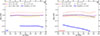 |
Fig. 8. Dependence of the modulation phase Φgl on input physics as a function of Δν. The relative difference ΔΦgl = Φgl, mod − Φgl, ref, where Φgl, ref and Φgl, mod are the modulation phases found in the reference and modified models, is shown for 0.5 μHz wide Δν bins between 0.1 μHz and 4.0 μHz (except for the first Δν bin that is [0.1, 0.5] μHz). The reference model is defined with 1.75 M⊙ and solar metallicity, and the input physics are those indicated in Table 1. The settings of the modified models are similar to those of the reference models, except for one parameter, which is changed as indicated on the labels. (a) and (b) are obtained on the RGB and clump stage plus AGB, respectively. |
Given the strong effects of rotation on the glitch signature, we investigated other input physics that would generate efficient mixing in stellar interiors, for both the 1.0 M⊙ (Fig. B.2) and 1.75 M⊙ (Fig. 8) models. Envelope overshooting, which affects the composition of the envelope from the main sequence, has weak effects on Φgl, as shown in Figs. 8, B.2 (thick dot-dashed black line; the changes induced by considering envelope overshooting in the models barely exceed 0.2 rad). Therefore, no negative phase difference between He- and H-shell burning stars could be obtained. Similar conclusions can be drawn when considering extra mixing in the core. Core overshooting during the main sequence (dashed orange line) induces a similar phase shift, ΔΦgl = Φgl, αov, H = 0.4 − Φgl, αov, H = 0.2, in both the H-shell and He-burning phases. This shift is more significant than that observed for a 1 M⊙ model, as expected (Fig. B.2). By contrast, overshooting during the core-He burning phase (thick pink line) only weakly affects Φgl (Fig. 8). Other mixing above the H-burning shell can be caused by thermohaline mixing (Cantiello & Langer 2010; Charbonnel & Lagarde 2010; Lagarde et al. 2011, 2012). We do not notice any significant impact on Φgl when adding thermohaline mixing to the models. For M ≥ 1.5 M⊙, the thermohaline mixing layer located above the H-burning shell is not able to join the H-burning shell with the convective envelope during the He-core burning phase. In such cases, the transfer of H-burning products into the stellar envelope by thermohaline mixing is inefficient.
Finally, changing the mixing-length parameter αMLT affects Φgl equally in the shell-H and the He-burning phases; the ΔΦgl = Φgl, αMLT = 1.62 − Φgl, αMLT = 1.92 in the shell-H burning phase is similar to that in the He-burning phase (see the thin dot-dashed red line in Figs. 8, B.2e+f). Further investigation is needed to quantify the importance of these mixing mechanisms in causing the phase shift of the glitch signature between H-shell and He-burning stars at high mass.
5.3. Validity of the asymptotic approach at low Δν
In stellar models, we were able to infer the frequencies of the pressure radial, dipole, and quadrupole modes in an efficient way down to Δν ∼ 0.09 μHz (equivalently νmax ∼ 0.5 μHz and R = 120 R⊙) with ADIPLS (see Fig. 3). This offers the opportunity to test the relevance of the asymptotic expansion at low Δν. In this approach, deviations from the asymptotic pattern caused by any sharp variation feature must be small compared to the asymptotic leading-order term, so that these deviations can be treated as perturbations to the asymptotic relation. Here, we treated the ionisation-induced dip of Γ1 as a structural perturbation to a reference model in the absence of the effects of helium ionisation on the stellar structure (Gough 2002; Houdayer et al. 2021). As a consequence, the glitch signature in Δν (Eq. 10) was assumed to be a perturbation to the asymptotic expansion (Houdek & Gough 2007; Houdayer et al. 2022). Accordingly, we expected the amplitude of the glitch signature to be small with respect to Δν. In our analysis, we identified the asymptotic expansion to be quantitatively inaccurate when Δν ≤ 0.5 μHz. The reason for this breakdown is twofold. Firstly, the amplitude 𝒜gl of the glitch modulation becomes larger than 0.1 when Δν ≤ 0.5 μHz (Fig. 5a), and eventually reaches 0.5 at the RGB tip, corresponding to a modulation amplitude equal to half the value of Δν4. At the same time, the amplitude of the dip, HHeII, in the Γ1 profile is larger and its extent, bHeII, is narrower, resulting in a sharper variation of Γ1 (see Figs. 5c+d). Secondly, the glitch signature has a significant effect on the local measurement of ε. This signature noticeably affects the profile of ε around Δν ∼ 0.7 μHz (see Fig. 4a). In this case, the perturbation approach cannot be adapted at low Δν. This conclusion is supported by observational results. The amplitude of the glitch modulation  introduced in the local large separation Δνn, ℓ at Δν = 0.8 μHz in Kepler observations is ∼0.07 Δν on the RGB and ∼0.08 Δν on the AGB (Dréau et al. 2021).
In addition to the large glitch amplitude at low Δν, the asymptotic expansion of the mode frequencies cannot be valid below Δν ≤ 0.5 μHz (equivalently νmax ≤ 2 μHz) because the assumption n ≫ ℓ is not fulfilled. In Dréau et al. (2021), we encountered difficulties to match the observed and the template oscillation spectra based on the asymptotic relation given by Eq. (1) when Δν ≤ 0.5 μHz. At the optimal value of Δν that maximises the cross correlation between the observed and template oscillation spectra, the observed and modelled modes do not overlap for all radial orders n. This reflects that the asymptotic expansion is not suitable to accurately reproduce the oscillation spectrum of red giants when Δν ≤ 0.5 μHz5.
Eventually, both the asymptotic expansion and the perturbation approach of the signature of HeII are not accurate when Δν ≤ 0.5 μHz. The efficiency of the classification method based on the signature of the HeII zone may not only be affected by the insufficient frequency resolution at low Δν, but also by the inadequate scheme to derive p-mode frequencies. Accordingly, a better suited framework to interpret the oscillation spectrum of high-luminosity red giants with Δν ≤ 0.5 μHz is necessary.
6. Conclusion
The unprecedented high-precision photometric data collected by Kepler provide access to seismic parameters, which are of major importance to constrain physical mechanisms in stellar interiors from early to late evolutionary stages. In this work, we physically interpreted the observed seismic parameters of high-luminosity red giants on the RGB and AGB in terms of structure parameters by means of stellar models. We computed a grid of stellar models with the stellar evolution code MESA, using different input physics such as overshooting, thermohaline mixing, and mass loss. Subsequently, we computed the non-radial mode frequencies in red giant evolved models (Δν ≤ 4 μHz) with the stellar oscillation code ADIPLS by adopting the squared Brunt–Väisälä frequency  equal to zero in the core (Ball et al. 2018). This method suppresses the g modes in the core, removing the need to compute mixed modes in red giant models, which would otherwise require tens of thousands of meshpoints to resolve their eigenmodes. However, unlike the original approach, it retains an inconsistent Γ1 profile. We verified that this method, inspired by Ball et al. (2018) and originally applied to non-radial mode frequencies in RGB stars with Δν ≤ 4.5 μHz, is also valid for non-radial modes in clump and AGB stars. In these cases, it introduces a possible bias of 0.02Δν and deviations of 0.03Δν − 0.04Δν for dipole modes, and a deviation of 0.02Δν for quadrupole modes. By combining these non-radial modes with the radial modes obtained without modifying the Brunt–Väisälä frequency down to νmax ∼ 0.1 μHz (equivalently, Δν ∼ 0.06 μHz), we computed the seismic parameters of the asymptotic pattern and the glitch signature. Thus, we were able to explore their dependence on the input physics and structure parameters output by MESA. The most impactful parameters are those modifying the physical conditions and composition of the envelope. The stellar mass M and metallicity [Fe/H] are the predominant parameters that influence the seismic parameters. The mixing-length parameter αMLT, the mass-loss rate on the RGB ηR, and the initial helium abundance Y0 have moderate impact on the asymptotic and glitch parameters, while the presence of extra-mixing regions, such as overshooting and thermohaline mixing, have minor influence.
The strength of the Γ1 variation in the HeII ionisation region correlates with the average temperature and density in this zone. Among these two parameters, the density difference is predominant when comparing RGB and AGB stars. This leads to a distinct modification of the helium ionisation zone, which in turn explains why the amplitude of the glitch signature is stronger in AGB stars than in RGB stars. This result extends previous findings established between RGB and clump stars (Christensen-Dalsgaard et al. 2014).
We verified that the asymptotic approach is not valid when Δν ≤ 0.5 μHz. Below this limit, the amplitude of the glitch signature is larger than 0.1 in units of Δν, showing that the glitch signature cannot be treated as a perturbation to the asymptotic relation. Moreover, the asymptotic relation does not suitably reproduce the observed pattern of modes when Δν ≤ 0.5 μHz, since the non-radial modes get closer to the neighbouring radial mode, forming a tightly packed triplet of modes. Accordingly, a suitable expression that includes the substantial glitch signature is required to describe the p-mode pattern towards low Δν.
The HeII zone is located closer to the surface in high-mass stars and progressively shifts inwards as Δν decreases. In fact, these stars have larger effective temperatures at fixed Δν, meaning that the temperature threshold for helium ionisation is reached closer to the surface. At low mass (M ≤ 1.5 M⊙), we recovered the phase difference between RGB and clump plus AGB stars in the glitch signature, which allowed us to identify the evolutionary status of red giants (Vrard et al. 2015; Dréau et al. 2021). We identified mass loss as the main cause of this phase difference, as the seismic parameters are mostly sensitive to the stellar mass. At high mass (M ≥ 1.5 M⊙), mass loss has minimal effect, but we found evidence that this phase difference can be retrieved by taking rotational-induced mixing into account. Henceforth, a combination of these input physics could allow us to reproduce this phase difference, which is found to be ∼ − 1.0 rad between clump plus AGB and RGB stars.
An accurate expression for the p-mode frequencies when Δν ≤ 0.5 μHz would not only facilitate mode identification in observations but also improve the efficiency of the classification methods. Indeed, the identification of evolutionary stages for red giants, which is based on the glitch signature (Kallinger et al. 2012; Vrard et al. 2015), assumes that the asymptotic relation is valid. In addition to being affected by the frequency resolution, the uncertainties in the evolutionary stages are influenced by the deviations from the asymptotic regime, which explains the increasing disagreements between different identification methods at low Δν. Eventually, our investigation into the physical mechanisms producing the phase difference between RGB and clump plus AGB stars in the glitch signature when M ≥ 1.5 M⊙ could be expanded. Our exploratory tests suggest that this phase difference may be recovered by considering any additional input physics that have the potential to change the physical conditions and composition of the envelope, where the HeII zone lies.
Acknowledgments
The authors warmly thank the anonymous referee for their valuable comments, which helped improve the depth of the discussion and the overall clarity of the manuscript. The authors also express their sincere thanks to the Kepler team for their tireless efforts in making high-precision data accessible, which have been instrumental in making these results possible. G.D. gratefully acknowledges support from the Australian Research Council through Discovery Project DP190100666. D.S. is supported by the Australian Research Council (DP190100666).
References
- Baglin, A., Auvergne, M., Barge, P., et al. 2006, ESA Spec. Publ., 1306, 33 [Google Scholar]
- Ball, W. H., Themeßl, N., & Hekker, S. 2018, MNRAS, 478, 4697 [Google Scholar]
- Baudin, F., Barban, C., Goupil, M. J., et al. 2012, A&A, 538, A73 [NASA ADS] [CrossRef] [EDP Sciences] [Google Scholar]
- Bedding, T. R., Huber, D., Stello, D., et al. 2010, ApJ, 713, L176 [Google Scholar]
- Bedding, T. R., Mosser, B., Huber, D., et al. 2011, Nature, 471, 608 [Google Scholar]
- Blocker, T. 1995, A&A, 297, 727 [Google Scholar]
- Borucki, W. J., Koch, D., Basri, G., et al. 2010, Science, 327, 977 [Google Scholar]
- Bossini, D., Miglio, A., Salaris, M., et al. 2015, MNRAS, 453, 2290 [Google Scholar]
- Bossini, D., Miglio, A., Salaris, M., et al. 2017, MNRAS, 469, 4718 [Google Scholar]
- Broomhall, A.-M., Miglio, A., Montalbán, J., et al. 2014, MNRAS, 440, 1828 [NASA ADS] [CrossRef] [Google Scholar]
- Cantiello, M., & Langer, N. 2010, A&A, 521, A9 [NASA ADS] [CrossRef] [EDP Sciences] [Google Scholar]
- Charbonnel, C., & Lagarde, N. 2010, A&A, 522, A10 [CrossRef] [EDP Sciences] [Google Scholar]
- Charbonnel, C., & Zahn, J. P. 2007, A&A, 467, L15 [NASA ADS] [CrossRef] [EDP Sciences] [Google Scholar]
- Choi, J., Dotter, A., Conroy, C., et al. 2016, ApJ, 823, 102 [Google Scholar]
- Christensen-Dalsgaard, J. 2008, Ap&SS, 316, 113 [Google Scholar]
- Christensen-Dalsgaard, J., Kjeldsen, H., & Mattei, J. A. 2001, ApJ, 562, L141 [Google Scholar]
- Christensen-Dalsgaard, J., Silva Aguirre, V., Elsworth, Y., & Hekker, S. 2014, MNRAS, 445, 3685 [Google Scholar]
- Corsaro, E., De Ridder, J., & García, R. A. 2015, A&A, 578, A76 [NASA ADS] [CrossRef] [EDP Sciences] [Google Scholar]
- Cowling, T. G. 1941, MNRAS, 101, 367 [NASA ADS] [Google Scholar]
- Cunha, M. S., & Metcalfe, T. S. 2007, ApJ, 666, 413 [NASA ADS] [CrossRef] [Google Scholar]
- Deheuvels, S., Brandão, I., Silva Aguirre, V., et al. 2016, A&A, 589, A93 [NASA ADS] [CrossRef] [EDP Sciences] [Google Scholar]
- Dréau, G., Mosser, B., Lebreton, Y., Gehan, C., & Kallinger, T. 2021, A&A, 650, A115 [NASA ADS] [CrossRef] [EDP Sciences] [Google Scholar]
- Dréau, G., Lebreton, Y., Mosser, B., Bossini, D., & Yu, J. 2022, A&A, 668, A115 [NASA ADS] [CrossRef] [EDP Sciences] [Google Scholar]
- Dziembowski, W. A., Gough, D. O., Houdek, G., & Sienkiewicz, R. 2001, MNRAS, 328, 601 [Google Scholar]
- Eggleton, P. P., Dearborn, D. S. P., & Lattanzio, J. C. 2006, Science, 314, 1580 [Google Scholar]
- Eggleton, P. P., Dearborn, D. S. P., & Lattanzio, J. C. 2008, ApJ, 677, 581 [NASA ADS] [CrossRef] [Google Scholar]
- Farnir, M., Dupret, M. A., Salmon, S. J. A. J., Noels, A., & Buldgen, G. 2019, A&A, 622, A98 [NASA ADS] [CrossRef] [EDP Sciences] [Google Scholar]
- Gilliland, R. L., Brown, T. M., Christensen-Dalsgaard, J., et al. 2010, PASP, 122, 131 [Google Scholar]
- Gough, D. O. 1986, Highlights Astron., 7, 283 [Google Scholar]
- Gough, D. O. 1990, in Comments on Helioseismic Inference, eds. Y. Osaki, & H. Shibahashi, 367, 283 [Google Scholar]
- Gough, D. O. 2002, ESA Spec. Publ., 485, 65 [Google Scholar]
- Henyey, L., Vardya, M. S., & Bodenheimer, P. 1965, ApJ, 142, 841 [Google Scholar]
- Hon, M., Stello, D., & Yu, J. 2017, MNRAS, 469, 4578 [NASA ADS] [CrossRef] [Google Scholar]
- Hon, M., Stello, D., & Yu, J. 2018, MNRAS, 476, 3233 [NASA ADS] [CrossRef] [Google Scholar]
- Houdayer, P. S., Reese, D. R., Goupil, M.-J., & Lebreton, Y. 2021, A&A, 655, A85 [NASA ADS] [CrossRef] [EDP Sciences] [Google Scholar]
- Houdayer, P. S., Reese, D. R., & Goupil, M.-J. 2022, A&A, 663, A60 [NASA ADS] [CrossRef] [EDP Sciences] [Google Scholar]
- Houdek, G., & Gough, D. O. 2007, MNRAS, 375, 861 [CrossRef] [Google Scholar]
- Howell, S. B., Sobeck, C., Haas, M., et al. 2014, PASP, 126, 398 [Google Scholar]
- Huang, W., Gies, D. R., & McSwain, M. V. 2010, ApJ, 722, 605 [Google Scholar]
- Huber, D., Bedding, T. R., Stello, D., et al. 2010, ApJ, 723, 1607 [NASA ADS] [CrossRef] [Google Scholar]
- Huber, D., Bedding, T. R., Stello, D., et al. 2011, ApJ, 743, 143 [Google Scholar]
- Iglesias, C. A., & Rogers, F. J. 1996, ApJ, 464, 943 [NASA ADS] [CrossRef] [Google Scholar]
- Kallinger, T., Hekker, S., Mosser, B., et al. 2012, A&A, 541, A51 [NASA ADS] [CrossRef] [EDP Sciences] [Google Scholar]
- Kallinger, T., Beck, P. G., Stello, D., & Garcia, R. A. 2018, A&A, 616, A104 [NASA ADS] [CrossRef] [EDP Sciences] [Google Scholar]
- Khan, S., Hall, O. J., Miglio, A., et al. 2018, ApJ, 859, 156 [NASA ADS] [CrossRef] [Google Scholar]
- Khan, S., Miglio, A., Mosser, B., et al. 2019, A&A, 628, A35 [NASA ADS] [CrossRef] [EDP Sciences] [Google Scholar]
- Kippenhahn, R., Ruschenplatt, G., & Thomas, H. C. 1980, A&A, 91, 175 [Google Scholar]
- Kjeldsen, H., & Bedding, T. R. 1995, A&A, 293, 87 [NASA ADS] [Google Scholar]
- Lagarde, N., Charbonnel, C., Decressin, T., & Hagelberg, J. 2011, A&A, 536, A28 [NASA ADS] [CrossRef] [EDP Sciences] [Google Scholar]
- Lagarde, N., Decressin, T., Charbonnel, C., et al. 2012, A&A, 543, A108 [NASA ADS] [CrossRef] [EDP Sciences] [Google Scholar]
- Langer, N., El Eid, M. F., & Fricke, K. J. 1985, A&A, 145, 179 [NASA ADS] [Google Scholar]
- Lebreton, Y., & Goupil, M. J. 2012, A&A, 544, L13 [NASA ADS] [CrossRef] [EDP Sciences] [Google Scholar]
- Lopes, I., Turck-Chieze, S., Michel, E., & Goupil, M.-J. 1997, ApJ, 480, 794 [NASA ADS] [CrossRef] [Google Scholar]
- Maeder, A. 1975, A&A, 40, 303 [NASA ADS] [Google Scholar]
- Marigo, P., & Aringer, B. 2009, A&A, 508, 1539 [CrossRef] [EDP Sciences] [Google Scholar]
- Mazumdar, A., Michel, E., Antia, H. M., & Deheuvels, S. 2012, A&A, 540, A31 [NASA ADS] [CrossRef] [EDP Sciences] [Google Scholar]
- Mazumdar, A., Monteiro, M. J. P. F. G., Ballot, J., et al. 2014, ApJ, 782, 18 [NASA ADS] [CrossRef] [Google Scholar]
- Meynet, G., & Maeder, A. 1997, A&A, 321, 465 [NASA ADS] [Google Scholar]
- Michaud, G., Richer, J., & Richard, O. 2010, A&A, 510, A104 [NASA ADS] [CrossRef] [EDP Sciences] [Google Scholar]
- Miglio, A., Montalbán, J., Carrier, F., et al. 2010, A&A, 520, L6 [CrossRef] [EDP Sciences] [Google Scholar]
- Miglio, A., Brogaard, K., Stello, D., et al. 2012, MNRAS, 419, 2077 [Google Scholar]
- Miglio, A., Chiappini, C., Mackereth, J. T., et al. 2021, A&A, 645, A85 [NASA ADS] [CrossRef] [EDP Sciences] [Google Scholar]
- Montalbán, J., Miglio, A., Noels, A., Scuflaire, R., & Ventura, P. 2010, ApJ, 721, L182 [Google Scholar]
- Montalbán, J., Miglio, A., Noels, A., et al. 2012, Red Giants as Probes of the Structure and Evolution of the Milky Way (Berlin, Heidelberg: Springer-Verlag), 23 [Google Scholar]
- Monteiro, M. J. P. F. G., & Thompson, M. J. 2005, MNRAS, 361, 1187 [NASA ADS] [CrossRef] [Google Scholar]
- Monteiro, M. J. P. F. G., Christensen-Dalsgaard, J., & Thompson, M. J. 1994, A&A, 283, 247 [NASA ADS] [Google Scholar]
- Mosser, B., Belkacem, K., Goupil, M., et al. 2011, A&A, 525, L9 [CrossRef] [EDP Sciences] [Google Scholar]
- Mosser, B., Dziembowski, W. A., Belkacem, K., et al. 2013a, A&A, 559, A137 [CrossRef] [EDP Sciences] [Google Scholar]
- Mosser, B., Michel, E., Belkacem, K., et al. 2013b, A&A, 550, A126 [CrossRef] [EDP Sciences] [Google Scholar]
- Mosser, B., Michel, E., Samadi, R., et al. 2019, A&A, 622, A76 [NASA ADS] [CrossRef] [EDP Sciences] [Google Scholar]
- Paxton, B., Bildsten, L., Dotter, A., et al. 2011, ApJS, 192, 3 [Google Scholar]
- Paxton, B., Cantiello, M., Arras, P., et al. 2013, ApJS, 208, 4 [Google Scholar]
- Paxton, B., Marchant, P., Schwab, J., et al. 2015, ApJS, 220, 15 [Google Scholar]
- Paxton, B., Schwab, J., Bauer, E. B., et al. 2018, ApJS, 234, 34 [NASA ADS] [CrossRef] [Google Scholar]
- Paxton, B., Smolec, R., Schwab, J., et al. 2019, ApJS, 243, 10 [Google Scholar]
- Pinsonneault, M. H., Elsworth, Y. P., Tayar, J., et al. 2018, ApJS, 239, 32 [Google Scholar]
- Reimers, D. 1975, Mem. Soc. Roy. Sci. Liege, 8, 369 [Google Scholar]
- Ricker, G. R., Winn, J. N., Vanderspek, R., et al. 2015, J. Astron. Telesc. Instrum. Syst., 1, 014003 [Google Scholar]
- Roxburgh, I. W., & Vorontsov, S. V. 2003, A&A, 411, 215 [NASA ADS] [CrossRef] [EDP Sciences] [Google Scholar]
- Scherrer, P. H., Wilcox, J. M., Christensen-Dalsgaard, J., & Gough, D. O. 1983, Sol. Phys., 82, 75 [Google Scholar]
- Shibahashi, H., & Osaki, Y. 1981, PASJ, 33, 713 [Google Scholar]
- Stello, D., Compton, D. L., Bedding, T. R., et al. 2014, ApJ, 788, L10 [NASA ADS] [CrossRef] [Google Scholar]
- Tassoul, M. 1980, ApJS, 43, 469 [Google Scholar]
- Trabucchi, M., Wood, P. R., Montalbán, J., et al. 2017, ApJ, 847, 139 [Google Scholar]
- Ulrich, R. K. 1972, ApJ, 172, 165 [NASA ADS] [CrossRef] [Google Scholar]
- Unno, W., Osaki, Y., Ando, H., Saio, H., & Shibahashi, H. 1989, Nonradial Oscillations of Stars (Tokyo: University of Tokyo Press) [Google Scholar]
- Verma, K., Faria, J. P., Antia, H. M., et al. 2014, ApJ, 790, 138 [Google Scholar]
- Verma, K., Raodeo, K., Basu, S., et al. 2019, MNRAS, 483, 4678 [Google Scholar]
- Vorontsov, S. V. 1988, IAU Symp., 123, 151 [Google Scholar]
- Vorontsov, S. V., Baturin, V. A., & Pamiatnykh, A. A. 1992, MNRAS, 257, 32 [NASA ADS] [CrossRef] [Google Scholar]
- Vrard, M., Mosser, B., Barban, C., et al. 2015, A&A, 579, A84 [CrossRef] [EDP Sciences] [Google Scholar]
- Vrard, M., Mosser, B., & Samadi, R. 2016, A&A, 588, A87 [CrossRef] [EDP Sciences] [Google Scholar]
- White, T. R., Bedding, T. R., Stello, D., et al. 2011, ApJ, 743, 161 [Google Scholar]
- Yu, J., Bedding, T. R., Stello, D., et al. 2020, MNRAS, 493, 1388 [Google Scholar]
- Yu, J., Hekker, S., Bedding, T. R., et al. 2021, MNRAS, 501, 5135 [NASA ADS] [CrossRef] [Google Scholar]
- Zahn, J. P. 1991, A&A, 252, 179 [Google Scholar]
Located at $MESA_DIR/star/test_suite/1M_pre_ms_to_wd after downloading from https://zenodo.org/records/3698354
Located at $MESA_DIR/star/test_suite/1.5M_with_diffusion after downloading from https://zenodo.org/records/3698354
The computations used to derive this relation are presented in Appendix A of Dréau et al. (2021).
We recall that 𝒜gl is a dimensionless parameter expressed as a fraction of Δν, as depicted by Eq. (10).
We note that the frequency resolution of Kepler observations is insufficient for a comprehensive seismic study of red giants with Δν ≤ 0.5 μHz; nevertheless, the mode frequencies can be correctly inferred (Mosser et al. 2013a; Yu et al. 2020).
Appendix A: Mass dependence of the glitch modulation period 𝒢gl
Stellar models highlight a noticeable mass dependence on the modulation period 𝒢gl (Fig. 6a+b). Then, we inspect how this glitch parameter varies with mass in Kepler observations. This part supplements the observational results presented in Dréau et al. (2021). To summarise, the frequency large separation Δν is obtained as the value that optimises the cross correlation between the observed oscillation spectrum and the template spectrum based on the asymptotic relation of p-mode frequencies in red giants (Eq. 1). The way the modulation period 𝒢gl is extracted is similar to that described in Sect. 3.3, except that the fit of the glitch signature is limited to the observed mode frequencies. Stellar masses are assessed from the semi-empirical asteroseismic scaling relation presented in Kjeldsen & Bedding (1995). Deviations from the asteroseismic scaling relations are corrected by a factor that is adjusted star by star (Pinsonneault et al. 2018). When this correcting factor is not available, which concerns about 10% of our Kepler targets, we estimated the mass with the semi-empirical relation without any correction factor. In Fig. A.1, we show the mass dependence of the modulation period 𝒢gl as a function of Δν, from the dataset used in Dréau et al. (2021), including ∼ 2,100 RGB, clump and AGB stars. We note that low-mass stars (M ≤ 1.2 M⊙) tend to have a lower modulation period 𝒢gl compared to their higher-mass counterparts (M ≥ 1.2 M⊙) at fixed Δν. This means that the helium ionisation occurs closer to the surface when the stellar mass increases. These observations are in line with the results obtained with stellar models, presented in Sect. 4.3.2. The effective temperature Teff is higher in high-mass stars, which makes the physical conditions for helium ionisation to be reached closer to the surface, resulting a larger modulation period 𝒢gl.
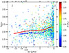 |
Fig. A.1. Glitch modulation period derived from the Kepler data used in Dréau et al. (2021) as a function of Δν, where the stellar mass is colour-coded. Mean error bars estimated for Δν below or above 1 μHz are represented. The thick solid lines are the median values in bins of 0.5 μHz Δν, regardless of the evolutionary stage, shown in blue for low-mass stars (M ≤ 1.2 M⊙) and in red for high-mass stars (M ≥ 1.2 M⊙). |
Appendix B: Effects of input physics on seismic parameters
We aim at investigating the effects of stellar parameters and input physics on seismic parameters. To this end, we generated a grid of stellar models based on the reference model of mass 1 M⊙ and solar metallicity presented in Table 1. We changed the input physics relative to the reference model and compared the seismic parameters between the reference and modified models in several bins of Δν. In order to smooth the evolutionary tracks, we computed the median values of seismic parameters every three consecutive models and kept the average values in 0.5 μHz wide Δν bins. These averaged values obtained in the modified models, noted Xmod, are then compared to those of the reference model, noted Xref, by means of the relative difference
 (B.1)
(B.1)
Here, X can be the acoustic offset ε, the dimensionless small frequency separations d01 and d02, the modulation amplitude 𝒜gl and period 𝒢gl. For the modulation phase Φgl, we directly compare the reference and modified models with the absolute difference ΔΦgl = Φgl, mod − Φgl, ref.
From Figs. B.1; B.2; and B.3, we can infer the impact of input physics on seismic parameters and HeII ionisation zone characteristics as a function of the evolutionary stage.
B.1. Mass, mass loss, and metallicity
The main parameters affecting the seismic quantities in Eqs. 1,10 are the stellar mass (varied from 1 M⊙ to 1.75 M⊙) and metallicity (from 0 dex to −1 dex), with relative differences exceeding 20% for some seismic parameters. Given the strong dependence of the seismic parameters on stellar mass M, we also expect the mass loss rate ηR to have an effect. Because most of the mass loss occurs near the luminosity-tip of the RGB, we investigate the effect only after He-burning starts. Modifying the mass loss rate, ηR, produces systematic shifts in both the seismic parameters from the asymptotic pattern (Eq. 1) and the glitch signature (Eq. 10) with respect to the reference value, with relative differences that could reach ∼5%. The most prominent effect of ηR is on the modulation phase Φgl, which likely accounts for the phase difference observed between RGB and clump plus AGB stars, as discussed in Sect. 5.2. Decreasing the mass loss parameter from ηR = 0.3 to 0.1 changes the mass difference between the initial and clump mass from 0.15 to 0.05 M⊙. Hence, the impact of mass loss on the seismic parameters remain small compared to the effect of changing the initial mass from, say, 1 to 1.75 M⊙.
B.2. Mixing length parameter
Varying the mixing-length parameter αMLT from 1.92 to 1.62 induces systematic shifts in both the asymptotic and the glitch signature parameters, with relative differences reaching up to ∼5% compared to the reference model. This adjustment particularly affects the acoustic offset ε and the modulation phase Φgl. It is expected, because ε is mostly affected by the envelope structure (Christensen-Dalsgaard et al. 2014), which the mixing length parameter affects (such as the effective temperature Teff and radius R.) This also justifies the effects of αMLT on the modulation phase Φgl, since a change in ε leads to a change in Δν through Eq. 14, especially the modulation phase (Vrard et al. 2015).
B.3. Initial helium abundance
While a change in initial helium abundance Y0 from 0.25 to 0.30 only weakly affects d0ℓ, it clearly impacts the glitch parameters, and ε. This is expected because the glitch signature explicitly depends on the helium abundance (Houdek & Gough 2007; Houdayer et al. 2021, 2022), which gives the opportunity to estimate the helium abundance in cool red giant stars (Broomhall et al. 2014; Verma et al. 2014, 2019). A change in 0.05 in Y0 induces an average modification of ∼10% of the modulation amplitude 𝒜gl (Fig. B.2a+b).
The noisy profiles of the modulation amplitude 𝒜gl could result from the method used to extract the p-mode frequencies, specifically by setting  in the core. Indeed, Fig. 1b+d shows that a deviation of 3%−4% of Δν from the exact pure p-mode frequency may be introduced into mode frequencies, which is significant relative to the amplitude of the glitch signature. At low Δν, we suspect the 𝒜gl to be affected by large uncertainties due to the computation of the glitch signature with Eq. 9. The expected value of Δνn according to Eq. 1 is certainly not the best reference to isolate the glitch signature at low Δν.
B.4. Overshooting and thermohaline convection
Processes such as core and envelope overshooting with typical efficiency values ranging from α = 0.2 to 0.5 (see labels of Fig. B.1), as well as thermohaline mixing only marginally affect the seismic parameters derived from asymptotic expressions. The effects do not exceed 3% of the reference values of ε and d0ℓ, which is below the typical uncertainty derived from observations. We expect core-H overshooting during the main sequence not to have a significant impact because the convective core is very small when M = 1.0 M⊙. We note that thermohaline convection with an efficiency parameter of αth = 2, representing a rather inefficient case, connects the H-burning shell to the convective envelope only during the high-luminosity stages of the RGB. This likely accounts for the absence of significant effects when including thermohaline convection in our models.
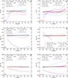 |
Fig. B.1. Sensitivity of seismic parameters in the asymptotic relation (Eq. 1) to the input physics of MESA models. The relative difference in seismic parameters given by Eq. B.1 between the reference and modified models is shown for 0.5 μHz-bins for Δν in the range [0.1, 4.0] μHz (except for the first Δν bin, which is [0.1, 0.5] μHz). The reference model is defined with 1 M⊙ and solar metallicity, and the input physics are those indicated in Table 1. The settings of the modified models are similar to those of the reference models, except for one parameter that is changed as indicated by the labels. The left and right columns correspond to the RGB and clump stage plus AGB, respectively. In panel d), some lines are shorter than the full range because the code failed to output the frequencies of ℓ = 1 modes when setting |

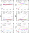 |
Fig. B.2. Sensitivity of the glitch parameters in the damped oscillator model (Eq. 10) to the input physics of MESA models. The labelling follows that in Fig. B.1, except that the modulation phase differences ΔΦgl between the reference and modified models are given by ΔΦgl = Φgl, mod − Φgl, ref, where Φgl, ref and Φgl, mod are the modulation phases found in the reference and modified models, respectively. |
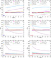 |
Fig. B.3. Sensitivity of the HeII zone parameters introduced in Eq. 12 to the input physics of MESA models. The same label is used as in Fig. B.1. |
All Tables
All Figures
|
Fig. 1. Comparison of the mode frequencies computed using the method |
| In the text | |
|
Fig. 2. (a) Profile of the first adiabatic exponent Γ1 as a function of the normalised acoustic radius in a 1 M⊙ RGB model computed with MESA at Δν = 1.65 μHz. The parameters of the Γ1 variations (HHeII, tHeII, and bHeII) are directly shown in the figure. The solid green line is the Γ1 profile throughout the star. The thick dashed orange line indicates the baseline that connects the local maximum after the dip caused by the second He-ionisation with the Γ1 profile before the dip. The thin dashed red line gives the fit of the Γ1 profile with Eq. (12) around the dip. (b) Glitch modulation induced by the second He-ionisation zone in the same model, as in the left panel. The local large separation Δνn, ℓ is shown in red circles, blue triangles, and green squares for radial, dipole, and quadrupole modes, respectively. The solid green line is the damped oscillator model given by Eq. (10) fitted to the data points. We point out that the data points are plotted at the mean frequencies (νn, ℓ + νn + 1, ℓ)/2. The upper x-axis indicates the radial order of ℓ = 0 modes, and the dotted blue line locates the maximum oscillation power. |
| In the text | |
|
Fig. 3. Model frequencies from radial order n = 1 up to n = 8 computed with ADIPLS for a 1 M⊙ track at solar metallicity. The MESA models are computed with the reference input physics listed in Table 1. Radial, dipole, and quadrupole modes are shown in red circles, blue triangles, and green squares, respectively. For the RGB (panel a), the grey frequencies are clump plus AGB models for comparison, and vice versa for the clump plus AGB (panel b). The non-radial modes (ℓ = 1, 2) are computed by setting the squared Brunt–Väisälä frequency |
| In the text | |
|
Fig. 4. Synthetic seismic parameters extracted from the p-mode frequencies computed with ADIPLS, as described in Sect. 3.3. The MESA models are computed with the reference input physics listed in Table 1, with M = 1.0 M⊙ and solar metallicity. (a) Variation of the acoustic offset ε as a function of Δν, with an emphasis on the evolutionary stage. Clump stars are shown by the orange ‘C’ symbols while the RGB and AGB are colour-coded in blue and red, respectively. ‘C’ symbols show the progress in the clump stage. Small (large, respectively), symbols correspond to the early (late, respectively), clump phase. The arrows indicate the direction of evolution. (b) and (c) Dimensionless small separations d0ℓ as a function of Δν. Mean error bars estimated for Δν below or above 0.5 μHz are represented on each panel. |
| In the text | |
|
Fig. 5. Synthetic glitch and structure parameters computed with MESA and ADIPLS. The MESA models are the same as those shown in Fig. 4. The glitch amplitude 𝒜gl and period 𝒢gl are shown on the (a) and (b) panels, respectively, while the amplitude HHeII and the width bHeII of the HeII zone in the Γ1 profile are exhibited on the (c) and (d) panels, respectively. The label matches that of Fig. 4. In panel b, the additional solid light grey line is the modulation period expected from the location of the HeII ionisation zone tHeII, which is computed according to Eq. (13). |
| In the text | |
|
Fig. 6. Synthetic glitch period 𝒢gl and phase Φgl computed with ADIPLS. The MESA models are computed with the reference input physics listed in Table 1. (a) Dependence of the modulation period 𝒢gl on the stellar mass as a function of Δν during the RGB. The mass in solar units is shown with different shades of grey. (b) Same as (a), but for 𝒢gl as a function of Teff. (c) Evolution of the modulation phase Φgl with Δν for models of initial mass 0.9 M⊙ at solar metallicity, with an emphasis on the evolutionary stage. The labelling is identical to that in Fig. 4. (d) Same as (c), but for models of initial mass 1.5 M⊙. |
| In the text | |
|
Fig. 7. (a) Dependence of the amplitude HHeII on the average temperature log THeII in the HeII zone. The input physics and label are the same as in Fig. 5 for models of mass 1 M⊙ and solar metallicity. Dotted lines show the log THeII − HHeII coordinates of the RGB and AGB models presented in the right panel. (b) Γ1 profiles on the RGB and AGB roughly at a similar Δν = 1.03 μHz. The arrows indicate the amplitude and the width of the Γ1 variation at the helium-second ionisation zone, in blue on the RGB and red on the AGB. (c) Same as panel a, but with the average density log ρHeII in the HeII zone instead of log THeII. (d) Logarithmic differences between the AGB and RGB models shown in (b) of the temperature (dot-dashed red line) and density (dashed green line) as a function of the normalised acoustic radius. The vertical solid and dashed lines indicate the location of the base of the convective envelope in the RGB and AGB models, respectively. |
| In the text | |
|
Fig. 8. Dependence of the modulation phase Φgl on input physics as a function of Δν. The relative difference ΔΦgl = Φgl, mod − Φgl, ref, where Φgl, ref and Φgl, mod are the modulation phases found in the reference and modified models, is shown for 0.5 μHz wide Δν bins between 0.1 μHz and 4.0 μHz (except for the first Δν bin that is [0.1, 0.5] μHz). The reference model is defined with 1.75 M⊙ and solar metallicity, and the input physics are those indicated in Table 1. The settings of the modified models are similar to those of the reference models, except for one parameter, which is changed as indicated on the labels. (a) and (b) are obtained on the RGB and clump stage plus AGB, respectively. |
| In the text | |
|
Fig. A.1. Glitch modulation period derived from the Kepler data used in Dréau et al. (2021) as a function of Δν, where the stellar mass is colour-coded. Mean error bars estimated for Δν below or above 1 μHz are represented. The thick solid lines are the median values in bins of 0.5 μHz Δν, regardless of the evolutionary stage, shown in blue for low-mass stars (M ≤ 1.2 M⊙) and in red for high-mass stars (M ≥ 1.2 M⊙). |
| In the text | |
|
Fig. B.1. Sensitivity of seismic parameters in the asymptotic relation (Eq. 1) to the input physics of MESA models. The relative difference in seismic parameters given by Eq. B.1 between the reference and modified models is shown for 0.5 μHz-bins for Δν in the range [0.1, 4.0] μHz (except for the first Δν bin, which is [0.1, 0.5] μHz). The reference model is defined with 1 M⊙ and solar metallicity, and the input physics are those indicated in Table 1. The settings of the modified models are similar to those of the reference models, except for one parameter that is changed as indicated by the labels. The left and right columns correspond to the RGB and clump stage plus AGB, respectively. In panel d), some lines are shorter than the full range because the code failed to output the frequencies of ℓ = 1 modes when setting |
| In the text | |
|
Fig. B.2. Sensitivity of the glitch parameters in the damped oscillator model (Eq. 10) to the input physics of MESA models. The labelling follows that in Fig. B.1, except that the modulation phase differences ΔΦgl between the reference and modified models are given by ΔΦgl = Φgl, mod − Φgl, ref, where Φgl, ref and Φgl, mod are the modulation phases found in the reference and modified models, respectively. |
| In the text | |
|
Fig. B.3. Sensitivity of the HeII zone parameters introduced in Eq. 12 to the input physics of MESA models. The same label is used as in Fig. B.1. |
| In the text | |
Current usage metrics show cumulative count of Article Views (full-text article views including HTML views, PDF and ePub downloads, according to the available data) and Abstracts Views on Vision4Press platform.
Data correspond to usage on the plateform after 2015. The current usage metrics is available 48-96 hours after online publication and is updated daily on week days.
Initial download of the metrics may take a while.