| Issue |
A&A
Volume 706, February 2026
|
|
|---|---|---|
| Article Number | A377 | |
| Number of page(s) | 9 | |
| Section | Cosmology (including clusters of galaxies) | |
| DOI | https://doi.org/10.1051/0004-6361/202555093 | |
| Published online | 20 February 2026 | |
The dependence of galaxy assembly bias on the selection criteria, number density, and redshift of galaxy samples
1
Departamento de Física de la Tierra y Astrofísica, Fac. de C.C. Físicas, Universidad Complutense de Madrid E-28040 Madrid, Spain
2
Institut de Física d’Altes Energies (IFAE), The Barcelona Institute of Science and Technology 08193 Bellaterra (Barcelona), Spain
★ Corresponding authors: This email address is being protected from spambots. You need JavaScript enabled to view it.
; This email address is being protected from spambots. You need JavaScript enabled to view it.
Received:
9
April
2025
Accepted:
5
January
2026
Abstract
One of the key factors influencing galaxy clustering in the nonlinear regime is galaxy assembly bias, which describes the dependence of galaxy clustering on halo properties beyond halo mass. We studied this effect by analyzing galaxy samples selected according to stellar mass, luminosity, and broadband colors from the IllustrisTNG hydrodynamical simulation. We find that galaxy assembly bias depends strongly on the selection criteria, number density, and redshift of the galaxy sample; this effect increases or decreases galaxy clustering by as much as 25%. Interestingly, no single secondary halo property fully captures the strength of galaxy assembly bias for any galaxy population. Therefore, empirical models predicting galaxy assembly bias as a function of a single halo property cannot reproduce predictions from hydrodynamical simulations. Finally, we investigated how galaxy assembly bias arises from the interplay between halo assembly bias (the dependence of halo clustering on properties other than halo mass) and occupancy variation (the correlation between galaxy occupation and secondary halo properties). We provide a fast analytical expression to predict the level of galaxy assembly bias induced by any halo property in simulated galaxy catalogs without the need for computationally expensive shuffling techniques.
Key words: galaxies: formation / galaxies: statistics / cosmology: theory / large-scale structure of Universe
© The Authors 2026
 Open Access article, published by EDP Sciences, under the terms of the Creative Commons Attribution License (https://creativecommons.org/licenses/by/4.0), which permits unrestricted use, distribution, and reproduction in any medium, provided the original work is properly cited.
This article is published in open access under the Subscribe to Open model. This email address is being protected from spambots. You need JavaScript enabled to view it. to support open access publication.
1. Introduction
Structure formation theories predict that galaxies form as gas cools and condenses within virialized dark matter structures known as halos (White & Rees 1978). Consequently, the formation, growth, and properties of galaxies are likely to be closely connected to the growth, internal properties, and distribution of halos. Small-scale measurements of galaxy clustering and galaxy-galaxy lensing are highly sensitive to this relationship, the galaxy-halo connection, making its thorough understanding crucial for cosmological analyses (Chaves-Montero et al. 2023; Contreras et al. 2023b).
Of the multiple effects affecting the galaxy–halo connection, we examine the dependence of galaxy clustering on halo properties beyond mass, an effect commonly known as galaxy assembly bias (Croton et al. 2007; Zentner et al. 2014). This effect is a prevalent prediction of the most advanced hydrodynamical simulations, including EAGLE (Chaves-Montero et al. 2016), Illustris (Artale et al. 2018), IllustrisTNG (Hadzhiyska et al. 2021b), and MillenniumTNG (Contreras et al. 2023a), as well as semi-analytic models, such as the precursor of SAGE (Croton et al. 2007; Contreras et al. 2021), L-GALAXIES (Zehavi et al. 2018; Contreras et al. 2019), Semi-Analytical Galaxies (Jimenez & Heavens 2020), and Santa Cruz (Hadzhiyska et al. 2021a). However, the strength of this effect depends on the properties of the galaxy sample and, for a particular galaxy sample, varies across galaxy formation models.
Detecting galaxy assembly bias in observations is inherently challenging as a direct detection would require unambiguously associating each galaxy with its host dark matter halo, and accurately estimating the mass of these halos. Both steps are difficult: assigning galaxies to halos is uncertain, and measuring individual halo masses at cosmological distances remains highly nontrivial (e.g., Zhao et al. 2025). Consequently, most observational analyses infer galaxy assembly bias indirectly by fitting empirical models to galaxy clustering data, where specific parameters govern the strength of assembly bias. A robust detection therefore requires an empirical model sufficiently flexible to capture all relevant astrophysical effects influencing galaxy clustering from intermediate to small scales; otherwise, the impact of these effects may be mistakenly interpreted as evidence of galaxy assembly bias. There is considerable disagreement in the literature regarding the detection of galaxy assembly bias; some studies report positive detections (e.g., Yuan et al. 2021; Wang et al. 2022; Yuan et al. 2022b; Contreras et al. 2023b; Alam et al. 2024; Paviot et al. 2024; Pearl et al. 2024), while others find no conclusive evidence for its presence (e.g., Zu & Mandelbaum 2018; Niemiec et al. 2018; Yuan et al. 2020; McCarthy et al. 2022; Yuan et al. 2022a). These inconsistencies are partly due to the fact that many analyses constrain only the model parameters governing assembly bias, rather than quantifying its percent-level effect on clustering, which complicates the interpretation because the link between parameter values and the actual magnitude of assembly bias is often nontrivial.
The primary goal of this work is to systematically quantify galaxy assembly bias for the galaxy populations most representative of large-scale structure surveys. Spectroscopic surveys such as the Sloan Digital Sky Survey (SDSS; York et al. 2000) and the Dark Energy Spectroscopic Instrument (DESI; DESI Collaboration 2016) typically target luminous red galaxies (LRGs) at intermediate redshift, emission line galaxies (ELGs) at higher redshift, and stellar mass-selected samples at low redshift. In contrast, weak-lensing surveys such as the Dark Energy Survey (DES; The Dark Energy Survey Collaboration 2005) and the Kilo-Degree Survey (KiDS; Asgari et al. 2021) generally select galaxies based on their brightness in a broad band. In this work, we quantify galaxy assembly bias as a function of redshift and number density for samples selected by stellar mass, r-band magnitude, and broadband colors, designed to emulate the aforementioned observational selection criteria.
To this end, we analyzed the largest hydrodynamical simulation of the IllustrisTNG suite (Springel et al. 2018; Marinacci et al. 2018; Naiman et al. 2018; Pillepich et al. 2018a; Nelson et al. 2018), which accurately reproduces the clustering of red and blue galaxies as a function of redshift, in good agreement with SDSS/DR7 observations across a wide range of stellar masses (Springel et al. 2018). We therefore expect its predictions for galaxy assembly bias to be more representative of the real Universe than those from other hydrodynamical or semi-analytic models that exhibit significant discrepancies in galaxy clustering. Consequently, this work presents the first systematic study of galaxy assembly bias across the main galaxy populations relevant for large-scale structure analyses, all within a galaxy formation model describing the clustering of these populations accurately.
In addition to measuring the level of galaxy assembly bias for these samples, we studied how galaxy assembly bias emerges from the interplay of halo assembly bias (HAB) (e.g., Gao et al. 2005; Wechsler et al. 2006; Gao & White 2007), which is the dependence of halo clustering on properties other than halo mass, and occupancy variation (Zehavi et al. 2018), which is the correlation between galaxy occupation and secondary halo properties. We present a fast and practical technique for estimating the level of galaxy assembly bias for a galaxy population associated with a given secondary halo property, relying solely on the median value of this property for the host halos of these galaxies and the level of HAB as a function of the target property. We validate this method using data from the IllustrisTNG simulation. The precision of this approach can be further improved by measuring HAB from a much larger gravity-only simulation, as HAB is largely independent of cosmology (Contreras et al. 2019).
This paper is organized as follows. In Section 2 we present the IllustrisTNG simulation and extract multiple galaxy samples from it. We measure the strength of galaxy assembly bias from these samples in Section 3, and we study the emergence of this effect from the interplay of HAB and occupancy variation in Section 4. We summarize our main findings and conclude in Section 5.
2. Simulation
In Sections 2.1, 2.2, and 2.3 we introduce the IllustrisTNG simulation, describe the galaxy samples extracted from this simulation, and outline the halo properties used to study galaxy assembly bias, respectively.
2.1. IllustrisTNG simulation
For this work we analyzed galaxy samples extracted from the TNG300-1 hydrodynamical simulation, the largest from the IllustrisTNG suite1 (Springel et al. 2018; Marinacci et al. 2018; Naiman et al. 2018; Pillepich et al. 2018a; Nelson et al. 2018). This simulation was performed using the moving-mesh code AREPO (Springel 2010), which tracks the joint evolution of dark matter, gas, stars, and supermassive black holes employing a comprehensive galaxy formation model (Weinberger et al. 2017; Pillepich et al. 2018b).
The TNG300-1 simulation evolved 25003 gas cells and an equal number of dark matter particles within a periodic box of 205 h−1 Mpc on a side adopting the Planck 2015 cosmology (Planck Collaboration XIII 2016). The initial masses of the gas tracers and dark matter particles were 0.7 × 10⁷ and 4.0 × 10⁷ h−1 M⊙, respectively. Halos were detected using a standard friends-of-friends group finder with a linking length of b = 0.2 (Davis et al. 1985), while self-bound substructures within halos, commonly known as subhalos, were identified with the SUBFIND algorithm (Springel et al. 2001; Dolag et al. 2009).
It is standard to refer to subhalos located at the potential minimum of their host halos as centrals, while other subhalos are designated as satellites. Central and satellite subhalos hosting a stellar component are identified as central or satellite galaxies, respectively. Some subhalos in the catalog were erroneously identified as independent halos by SUBFIND, leading to the misclassification of their galaxies as centrals instead of satellites. These subhalos are typically known as backsplash subhalos. We leveraged merger tree information to mitigate this problem, reclassifying backsplash subhalos as satellites and assigning them to the correct host halo.
We used the LHaloTree merger trees (Springel et al. 2005) to reclassify central subhalos at zi as satellites if they were identified as satellites for at least five snapshots from z = 3 to zi, where zi = 0, 0.5, 1, and 2 are the four snapshots we analyzed for this work. The five-snapshot threshold was chosen to mitigate transient tracking artifacts inherent to merger tree algorithms (e.g., Kong et al. 2025). Finally, we associated the reclassified subhalos with the last halos they interacted with, provided that the target halo mass exceeds that of the subhalo.
2.2. Galaxy samples
We analyzed galaxy assembly bias using galaxy samples selected according to stellar mass, r-band magnitude, and two samples based on broadband colors: blue and red. Specifically, we used stellar masses measured from all star particles bound to a subhalo and magnitudes resulting from the added luminosity of all these particles. We created versions of these four samples with number densities n = 0.01, 0.003, 0.001, and 0.0003 h3 Mpc−3 at z = 0, 0.5, 1, and 2. To produce each of the stellar mass and r-band samples, we selected galaxies with the greatest value of the corresponding property until reaching the target number density. We generated the blue and red samples by first selecting all galaxies in the position of the color–magnitude diagram roughly corresponding to galaxies with specific star formation rates greater and smaller than log10(sSFR [yr−1]) = −11, respectively (see Fig. 1). Then, for the blue and red samples, respectively, we selected the galaxies with the greatest star formation rate and r-band magnitude until we reached the target number density.
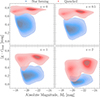 |
Fig. 1. Rest-frame color-magnitude diagram of TNG-300 galaxies with M★ > 109 h−1 M⊙. The results for galaxies with specific star formation rates greater and smaller than log10(sSFR [yr−1]) = −11 are shown in blue and red, respectively. The contours denote deciles of the populations; the darker shaded areas indicate the most densely populated regions. |
We only used galaxies with stellar mass greater than M★ = 109 h−1 M⊙, equivalent to more than 100 star particles, to generate these samples in order to ensure that all galaxies were sufficiently resolved. Furthermore, we did not produce the blue sample with n = 0.01 h3 Mpc−3, due to the limited resolution of the simulation, nor the red samples with n = 0.01 h3 Mpc−3 at all redshifts; n = 0.003 h3 Mpc−3 at z = 1 and 2; and n = 0.001 h3 Mpc−3 at z = 2, owing to its limited volume. In the left and right panels, respectively, of Figure 2 we show the halo and stellar mass functions of the 53 resulting samples. The host halos of all galaxies in the samples have masses greater than Mh = 1010 h−1 M⊙, corresponding to approximately 250 particles, which ensures that they are well resolved.
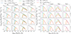 |
Fig. 2. Halo mass function (left panels) and stellar mass function (right panels) for the stellar mass, r-band, blue, and red samples. Each column corresponds to a different sample, while the rows represent the results at different redshifts. The colored lines show the mass functions for samples with distinct number densities. The black lines in the left panels display the halo mass function for Mh > 1010 h−1 M⊙ halos, while the purple lines in the right panels depict the stellar mass function M★ > 109 h−1 M⊙ galaxies. |
2.3. Halo samples
We measured the HAB for concentration, spin, and formation time using halos with masses greater than Mh = 1010 h−1 M⊙ at z = 0, 0.5, 1, and 2. In what follows, we describe these properties.
We estimated the concentration of dark matter halos as the ratio of the maximum circular velocity to  (Gao & White 2007), where M200 is the halo mass enclosed within a sphere of mean density 200 times the critical density of the Universe, R200 is the radius of this sphere, and G is the gravitational constant. Although more precise methods for estimating halo concentration exist (e.g., Child et al. 2018), our approach provides sufficient accuracy for ranking halos by concentration.
Following Bullock et al. (2001), we computed the halo spin as
 (1)
(1)
where J200 is the magnitude of the angular momentum within a sphere of radius R200. While the number of particles required to compute the halo spin accurately exceeds the 250 particle limit we imposed, the resulting estimates, though noisy, are sufficiently precise for ranking halos according to this property.
Finally, we defined the halo formation time, tf, as the cosmic lookback time at which a halo first attains half of its mass at each of the four redshifts used in this work. This property was measured from the TNG300 merger trees.
3. Measurements of galaxy assembly bias
We measured the level of galaxy assembly bias from simulated galaxy samples using the shuffling technique proposed by Croton et al. (2007). This method involves exchanging the galaxies hosted by each dark matter halo among halos of similar masses, effectively removing any clustering dependence on halo properties beyond halo mass. The level of galaxy assembly bias is quantified by comparing the clustering of the original galaxy sample with that of the shuffled sample. In what follows, we give more details about the shuffling procedure and present the level of galaxy assembly bias for each of the samples introduced in Sect. 2.2.
We began by dividing all halos into logarithmic halo mass bins with width Δ log10(Mh[h−1 M⊙]) = 0.15. We checked that using bins with slightly different sizes does not alter the results. We then calculated the relative distance between each galaxy and the center of potential of its host. Next, we shuffled the galaxies of all halos within each halo mass bin, while keeping the relative distances of galaxies to the halo center fixed, therefore preserving the one-halo term. Halos without galaxies are also included in the shuffling process. After that, we computed the two-point correlation function of both the unshuffled and shuffled samples, ξ and ξshfix Mh.
We employed the corrfunc (Sinha & Garrison 2020) package to compute the two-point correlation function, using 12 logarithmically spaced radial bins of width Δlog10(r[h−1 Mpc]) = 0.2 between r = 0.1 and 25 h−1 Mpc. To mitigate noise introduced by the stochastic nature of the shuffling technique, we computed 100 shufflings with different random seeds. We then calculated the median ratio of the clustering of the original sample to each shuffled catalog, ξ/ξshfix Mh, on scales from r = 8 to 25 h−1 Mpc. Finally, we estimated the level of galaxy assembly bias, along with its uncertainty, by computing the mean and standard deviation of the results for the 100 shufflings. We verified that further increasing the number of shufflings does not improve the results, and excluded larger scales in the calculation to minimize the influence of numerical artifacts, due to the simulation’s finite volume.
In Fig. 3 we display the level of galaxy assembly bias for galaxies selected by stellar mass with n = 0.003 h3 Mpc−3 at z = 0. The blue symbols and error bars display the mean and standard deviation of the ratio of the clustering of the original to the shuffled samples. This small-scale ratio approaches unity since the shuffling procedure preserves the relative distance between satellite galaxies, increases from r = 1 to ≃5 h−1 Mpc, and remains nearly constant for larger scales. We find a similar trend for other samples, number densities, and redshifts. This trend justifies using scales larger than 5 h−1 Mpc to measure the level of galaxy assembly bias, which is indicated by the blue horizontal line. The horizontal line is above unity, below unity, and at the same level if galaxy assembly bias is positive, negative, and null for a particular sample.
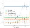 |
Fig. 3. Galaxy assembly bias for the stellar mass sample with number density n = 0.003 h3 Mpc−3 at z = 0. The blue symbols show the ratio of the clustering of this sample and of a modified version where galaxies are shuffled among halos of the same mass. The green, orange and red symbols show this ratio for modified versions of this sample where galaxies are shuffled among halos of the same mass and concentration, spin, and formation time, respectively. Horizontal lines display the average ratio on large scales, which corresponds to the level of galaxy assembly bias. The error bars and shaded areas indicate 1σ uncertainties. |
We then measured the level of galaxy assembly bias associated with halo concentration, spin, and formation time (see Sect. 2.3 for the definitions of these properties). Within each halo mass bin, we further subdivided halos into up to ten bins according to the selected secondary property, reducing the number of sub-bins only when a mass bin contains fewer than ten halos. We then shuffled the galaxy populations among halos within each sub-bin, effectively fixing both halo mass and the targeted secondary property (Xu et al. 2021). We verified that the results are stable against moderate variations in the number of sub-bins.
In Fig. 3, the green, orange, and red symbols show the ratio of the clustering of samples shuffled while holding fixed halo mass and concentration, spin, and formation time, respectively, and samples shuffled while only holding fixed halo mass. We display the results for the average of 100 shufflings. The colored horizontal lines indicate the galaxy assembly bias captured by each property; we computed these following the same approach as for computing the total assembly bias of the sample. If the galaxy assembly bias captured by a secondary property is greater than, equal to, or smaller than the total bias of the sample, the corresponding horizontal line is above, at the same level, and below the blue line, respectively. We find that concentration, spin, and formation time capture 37 ± 2%, 29 ± 2%, and 25 ± 2% of the total galaxy assembly bias of this sample, respectively. We note that our findings are compatible with the results from semi-analytic models (Xu et al. 2021).
For a more complete picture, in Fig. 4 we display the redshift evolution of galaxy assembly bias for the stellar mass, r-band, blue, and red galaxy samples (rows) with four distinct number densities (columns). The data points and error bars correspond to the horizontal lines and shaded areas of Fig. 3, respectively. The top panel of the second column displays the results for the stellar mass sample with a number density of n = 0.003 h3 Mpc−3, where the values at z = 0 correspond to the horizontal lines in Fig. 3. For this sample, the strength of galaxy assembly bias increases as redshift decreases, increasing from 1% at z = 2 to 17% at z = 0. To facilitate a comparison across samples and number densities, we overlay the results for this particular sample in all other panels.
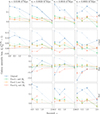 |
Fig. 4. Measurements of galaxy assembly bias captured by each secondary property from the stellar mass, r-band, blue, and red galaxy samples (rows) across different number densities (columns) as a function of redshift. The y-axis displays our measurements of galaxy assembly bias, which we extract by averaging from 8 to 25 h−1 Mpc the ratio of galaxy clustering of the sample shown in the legend and that of a modified version where galaxies are shuffled among halos of the same mass. In all panels, for ease of comparison, the symbols connected by dashed lines represent the results for the stellar mass sample with n = 0.003 h3 Mpc−3. The level of galaxy assembly bias varies significantly across samples, redshifts, and number density, increasing or decreasing galaxy clustering by as much as ≃24%. |
As we can see, the redshift evolution of galaxy assembly bias exhibits two primary trends, which depend on the nature of the sample and on its number density. The first trend is a steady increase in assembly bias with decreasing redshift, observed for the stellar mass and red galaxy samples with number densities greater or equal to n = 0.001 h3 Mpc−3. The second trend is a decline in assembly bias from z = 1 to 0, found for the remaining samples and number densities. As a result of this trend, the blue galaxy sample has a negative assembly bias for all number densities at z = 0, reaching –24% for the smallest number density considered. Consequently, the strength of the galaxy assembly bias depends strongly on the properties of the target galaxy population and can increase or decrease galaxy clustering up to 25%.
We can readily see that none of the secondary halo properties examined fully captures the galaxy assembly bias for all the galaxy samples. Interestingly, concentration and spin result in positive assembly bias in practically all cases, while formation time yields negative assembly bias for the r-band and blue galaxy samples. The correlation between galaxy clustering and halo formation time is therefore the most likely explanation of the negative assembly bias found for the blue galaxy sample.
4. Predicting galaxy assembly bias
In this section we discuss HAB and occupancy variation (Sects. 4.1 and 4.2, respectively) and how galaxy assembly bias emerges from their interplay (Sect. 4.3).
4.1. Halo assembly bias
The dependence of halo clustering on properties beyond halo mass is commonly known as HAB (e.g., Gao et al. 2005; Wechsler et al. 2006). Given that galaxy assembly bias refers to the dependence of galaxy clustering on halo properties beyond halo mass, HAB is a prerequisite for galaxy assembly bias. In the previous section we computed the fraction of galaxy assembly bias attributable to concentration, spin, and formation time for multiple samples; in this section, we quantify the strength of HAB for these properties.
Halo assembly bias has no redshift dependence beyond that captured by the evolution of the density field (e.g., Wechsler et al. 2006; Zentner 2007; Gao & White 2007). As a result, it is useful to combine the measurements of this effect from multiple redshifts to reduce the uncertainties owing to the limited volume of the TNG300 simulation. To do so, we started by computing the peak height corresponding to each halo of the snapshots at z = 0, 0.5, 1, and 2, ν = δc/σ(Mh), where δc = 1.686 is the linear overdensity threshold for collapse (Gunn & Gott 1972) and σ(Mh) is the variance of the density field. We carried out this calculation using the publicly available package colossus2. Then we split the halos from each snapshot into logarithmic bins of ν and selected samples containing 10, 20, 30, 40, 50, and 60% of the halos with the highest and lowest values of each secondary property from each bin. After that, we computed the clustering of subsamples with more than 3000 halos, as well as the clustering of all halos within each bin. We continued by computing the average ratio of the clustering of the subsamples and all halos within each bin from r = 8 to 25 h−1 Mpc. Finally, when we had data from multiple redshifts for a particular ν bin, we computed the average of the results from all these redshifts weighted by the number of halos.
In the left, central, and right panels of Fig. 5, we display the level of HAB for the subsamples with the 30% highest and lowest concentration, spin, and formation time, respectively. There is no HAB for a subsample when its clustering is the same as that of all halos, which is indicated by the dotted black line. As we can see, the dependence of HAB on halo mass is different for all properties. Low-mass halos with higher concentration are more clustered than their less concentrated counterparts, while the trend reverses for high-mass halos with peak height larger than log10ν ≃ 0.1. On the other hand, halos with larger spin and forming at an earlier time are more clustered.
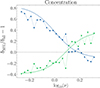 |
Fig. 5. Halo assembly bias for concentration (left), spin (center), and formation time (right). In each panel, the blue and green triangles display the HAB for the 30% of halos with the highest and lowest value of the corresponding property, respectively. The solid lines show the best-fitting model to the measurements (see text). |
In Sect. 4.3, we use the HAB measurements to predict the galaxy assembly bias. In order to mitigate the impact of statistical noise on these predictions, we approximate HAB measurements using the following empirically motivated expression
 (2)
(2)
where A, B, w, and ν0 are the free parameters of the model. For a subsample at a ν bin,  indicates the ratio of the median value of a particular halo property for this subsample to the median value for all halos. In Fig. 5, the solid lines display the predictions of the best-fitting model; as we can see, this model describes the data accurately. To remove the upturn of the spin HAB, we have to remove the backsplash halos and the halos with masses lower than 1010.75 M⊙, suggesting that the effect is also due to the resolution, in addition to the backsplash halos (Tucci et al. 2021).
4.2. Occupancy variation
Halo assembly bias is a necessary condition for galaxy assembly bias, but it is not sufficient. If we assume that the galaxy content of halos is independent of any property except for halo mass, galaxies would equally populate halos with values of the target property larger and smaller than average. As a result, the net HAB of the host halos could cancel out, resulting in no galaxy assembly bias for the galaxy population. On the other hand, if the galaxies of a particular sample preferentially populate older halos, for example, we would expect positive assembly bias given that the HAB for these halos is positive.
The dependence of the galaxy content of halos on secondary halo properties beyond halo mass is commonly known as occupancy variation, and it is common to study this effect by computing the occupation distribution of halos with different values of secondary properties (e.g., Zehavi et al. 2018; Artale et al. 2018; Contreras et al. 2019). In the top left, top right, bottom left, and bottom right panels of Fig. 6, the blue lines display the average halo occupation for the stellar mass, r-band, blue, and red samples with n = 0.003 h3 Mpc−3 at z = 0, respectively, while the green and orange lines show the halo occupation of the halos with the 30% highest and lowest concentration. For all samples, the probability of hosting satellites increases with halo mass, while the probability of hosting centrals increases with halo mass for all samples but the blue one, which decreases after peaking for low halo masses. This trend is explained by the fact that more massive halos typically host redder galaxies (e.g., Chaves-Montero & Hearin 2020).
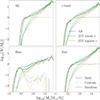 |
Fig. 6. In clockwise direction, halo occupation distribution for stellar mass, r-band, blue, and red galaxy samples with n = 0.003 h3 Mpc−3 at z = 0. The solid, dotted, and dashed lines show the results for all galaxies, centrals, and satellites, respectively. The results for the 25% of galaxies with the highest and lowest concentration are in orange and green, respectively, while the complete sample is in blue. We note that the occupancy of halos depends on the concentration for all galaxy samples. |
More interestingly, we find that low-mass halos with high concentration are more likely to host a central galaxy than those with low concentration for all samples, while the trend reverses for satellite galaxies and centrals in high-mass halos of the blue sample. Nevertheless, these dependencies are not very informative for the level of galaxy assembly bias of the sample. This is because galaxies could occupy halos with a mean value of a secondary property equal to that of all halos in the simulation; as a result, the HAB of the halos hosting galaxies would be zero. Furthermore, if the occupation content of these halos is symmetric for values of the target property higher and lower than the mean, the galaxy assembly bias of the sample could also be zero.
To better study the impact of occupancy variation on galaxy assembly bias, in Fig. 7 we display the ratio of the median concentration of halos hosting the galaxies of the samples shown in Fig. 6 to all the halos at this redshift,  . The value of
  is higher (lower) than unity if galaxies preferentially populate more (less) concentrated halos. The stellar mass, r-band, and red samples prefer to occupy more (less) concentrated halos with masses lower (higher) than Mh = 1012.6 h−1 M⊙. At z = 0, the HAB is positive for more (less) concentrated halos with masses lower (higher) than Mh = 1013.4 h−1 M⊙. As a result, the majority of the galaxies in these samples populate halos with a positive HAB, which explains the positive galaxy assembly bias of these samples. On the other hand, blue galaxies populate more (less) concentrated halos that are less (more) massive than Mh = 1011.75 h−1 M⊙. Consequently, the majority of the galaxies in this sample populate halos with negative HAB; as a result, the galaxy assembly bias of this sample is negative (see Fig. 4).
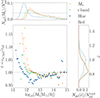 |
Fig. 7. Ratio of the median concentration of the halos hosting the stellar mass, r-band, blue and red galaxy samples with n = 0.003 h3 Mpc−3 at z = 0 to that of all halos at z = 0. The results for the stellar mass, r-band, blue and red galaxy samples are shown in orange, green, blue and red, respectively. The upper panel shows a histogram with the number of galaxies as a function of halo mass, while the right panel shows the median concentration of halos hosting different galaxy populations and all halos. |
In the next section we use occupancy variation measurements to predict galaxy assembly bias. In order to mitigate the impact of statistical noise, we approximate occupancy variation measurements using a Savitzky–Golay filter when the number of galaxies in a halo mass bin is smaller than 1000. The dotted lines display the resulting curves.
4.3. Predicting galaxy assembly bias
As discussed in the previous two sections, galaxy assembly bias emerges from the interplay of HAB and occupancy variation. In this section we provide an analytic expression to efficiently predict galaxy assembly bias as a function of these two effects without the need to employ computationally expensive shuffling techniques.
In the absence of galaxy assembly bias, the linear bias of a galaxy sample can be expressed as
 (3)
(3)
where bh(Mh) is the linear bias of a halo of mass Mh. We compute the halo bias using the Comparat et al. (2017) parameterization as implemented in colossus. We can modify the previous expression as follows to account for the galaxy assembly bias induced by a halo property x:
![Mathematical equation: $$ \begin{aligned} b_{\rm gal}^\mathrm{w/\ HAB}(\tilde{x}) = \frac{\int \mathrm{d} {M_{\mathrm{h} }} b_\mathrm{h} ({M_{\mathrm{h} }})[1 + \mathrm{HAB}({M_{\mathrm{h} }}, \tilde{x}({M_{\mathrm{h} }}))] N_{\rm gal}({M_{\mathrm{h} }})}{\int \mathrm{d} {M_{\mathrm{h} }} N_{\rm gal}({M_{\mathrm{h} }})}. \end{aligned} $$](/articles/aa/full_html/2026/02/aa55093-25/aa55093-25-eq8.gif) (4)
(4)
Here  is the ratio of the median value of the target halo property for halos containing galaxies to that of all halos as a function of halo mass (see Sect. 4.2), and
  is the strength of HAB as a function of halo mass and
  . We note that this expression deviates from Eq. (17) of Wechsler et al. (2006) since it does not require computing the distribution of galaxies and linear halo bias as a function of halo mass and property x, nor the probability of finding a halo of property x as a function of halo mass.
Combining the previous two equations allows us to compute the galaxy assembly bias induced by a halo property x:
 (5)
(5)
This expression provides a rapid estimate of galaxy assembly bias without relying on computationally expensive shuffling techniques. In order to improve the accuracy of this expression, we could measure the level of HAB for different halo properties from any large gravity-only simulation, given that galaxy assembly bias is largely insensitive to cosmology (Contreras et al. 2019).
In Fig. 8 we compare the measurements of the galaxy assembly bias induced by halo concentration, spin, and formation time obtained from the shuffling technique with predictions from the above expression. We show this comparison for all the samples, number densities, and redshifts analyzed in this work. As shown, Eq. (5) accurately reproduces the shuffling measurements for both positive and negative galaxy assembly bias, yielding a Pearson correlation coefficient of rp = 0.8. We therefore conclude that Eq. (5) provides an accurate prediction of the galaxy assembly bias produced by a given halo property.
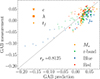 |
Fig. 8. Comparison between direct measurements of galaxy assembly bias from the shuffling procedure and predictions from our analytic model. The results for the stellar mass, r-band, blue, and red samples are shown in orange, green, blue and red, respectively, while the triangles, squares and dots indicate the galaxy assembly bias due to concentration, spin, and formation time. The dotted line indicates a 1 : 1 relation between measurements and predictions. We note that our analytic expression accurately predicts the amount of galaxy assembly bias resulting from the three studied halo properties, with a Pearson correlation greater than r = 0.8. |
5. Summary and conclusions
In this work, we studied the level of galaxy assembly bias for galaxy populations selected according to stellar mass, luminosity, and broadband colors from the largest hydrodynamical simulation from the IllustrisTNG suite. We summarize our main findings below:
-
In Fig. 4 we showed that the strength of galaxy assembly bias depends strongly on the selection criteria, number density, and redshift of the galaxy sample, increasing or decreasing clustering by as much as 25%.
-
The amount of galaxy assembly bias emerging from halo concentration, spin, and formation time does not fully explain the strength of this effect for any galaxy sample studied in this work. As a result, empirical approaches modeling galaxy assembly bias as a function of halo concentration or other single halo property cannot reproduce predictions from hydrodynamical simulations.
-
In Sect. 4 we provided an analytical expression to estimate the galaxy assembly bias induced by a halo property without having to resort to computationally expensive shuffling techniques. We validated that this expression accurately reproduces the level of galaxy assembly bias estimated by shuffling procedures, with a Pearson correlation coefficient greater than r = 0.8.
In this work we conducted a systematic analysis of galaxy assembly bias for galaxy samples with characteristics similar to those used for cosmological inference in state-of-the-art spectroscopic and photometric surveys. We find that the impact of galaxy assembly bias on galaxy clustering cannot be neglected for any galaxy sample, and thus it is crucial to account for this effect in the modeling of nonlinear scales for unbiased cosmological inference (e.g., Chaves-Montero et al. 2023; Contreras et al. 2023b).
To facilitate the modeling of galaxy assembly bias, we provide a fast analytical expression that predicts the level of galaxy assembly bias induced by any halo property, thus eliminating the need for computationally intensive shuffling techniques. This expression requires as input the level of HAB associated with a given halo property – measurable from any cosmological simulation – and the dependence of galaxy occupation on that property, which can be obtained from any galaxy-halo connection model. We envision using this framework to rapidly assess whether the level of galaxy assembly bias introduced by an empirical model is consistent with predictions from hydrodynamical simulations and semi-analytic models.
Acknowledgments
We thank the anonymous referee for the thorough review, insightful comments, and positive suggestions. We thank Sergio Contreras for useful comments and discussion, as well as the IllustrisTNG collaboration for making their data publicly available. JCM acknowledges support from the European Union’s Horizon Europe research and innovation programme (COSMO-LYA, grant agreement 101044612). We acknowledge the use of the Port d’Informació Científica (PIC) for the analysis, which is maintained through a collaboration agreement between the Institut de Física d’Altes Energies (IFAE) and the Centro de Investigaciones Energéticas, Medioambientales y Tecnológicas (CIEMAT). IFAE is partially funded by the CERCA program of the Generalitat de Catalunya. This work made direct use of the following software Python packages: Matplotlib (Hunter 2007), collossus (Diemer 2018), Corrfunc (Sinha & Garrison 2020), Numpy (Harris et al. 2020), Scipy (Virtanen et al. 2020), Seaborn (Waskom 2021), SciencPlots (Garrett et al. 2023) and pandas (McKinney 2010; The pandas development Team 2020).
References
- Alam, S., Paranjape, A., & Peacock, J. A. 2024, MNRAS, 527, 3771 [Google Scholar]
- Artale, M. C., Zehavi, I., Contreras, S., & Norberg, P. 2018, MNRAS, 480, 3978 [NASA ADS] [CrossRef] [Google Scholar]
- Asgari, M., Lin, C.-A., Joachimi, B., et al. 2021, A&A, 645, A104 [NASA ADS] [CrossRef] [EDP Sciences] [Google Scholar]
- Bullock, J. S., Dekel, A., Kolatt, T. S., et al. 2001, ApJ, 555, 240 [NASA ADS] [CrossRef] [Google Scholar]
- Chaves-Montero, J., & Hearin, A. 2020, MNRAS, 495, 2088 [NASA ADS] [CrossRef] [Google Scholar]
- Chaves-Montero, J., Angulo, R. E., Schaye, J., et al. 2016, MNRAS, 460, 3100 [NASA ADS] [CrossRef] [Google Scholar]
- Chaves-Montero, J., Angulo, R. E., & Contreras, S. 2023, MNRAS, 521, 937 [Google Scholar]
- Child, H. L., Habib, S., Heitmann, K., et al. 2018, ApJ, 859, 55 [NASA ADS] [CrossRef] [Google Scholar]
- Comparat, J., Prada, F., Yepes, G., & Klypin, A. 2017, MNRAS, 469, 4157 [NASA ADS] [CrossRef] [Google Scholar]
- Contreras, S., Zehavi, I., Padilla, N., et al. 2019, MNRAS, 484, 1133 [NASA ADS] [CrossRef] [Google Scholar]
- Contreras, S., Angulo, R. E., & Zennaro, M. 2021, MNRAS, 504, 5205 [CrossRef] [Google Scholar]
- Contreras, S., Angulo, R. E., Springel, V., et al. 2023a, MNRAS, 524, 2489 [NASA ADS] [CrossRef] [Google Scholar]
- Contreras, S., Chaves-Montero, J., & Angulo, R. E. 2023b, MNRAS, 525, 3149 [NASA ADS] [CrossRef] [Google Scholar]
- Croton, D. J., Gao, L., & White, S. D. M. 2007, MNRAS, 374, 1303 [Google Scholar]
- Davis, M., Efstathiou, G., Frenk, C. S., & White, S. D. M. 1985, ApJ, 292, 371 [Google Scholar]
- DESI Collaboration (Aghamousa, A., et al.) 2016, arXiv e-prints [arXiv:1611.00036] [Google Scholar]
- Diemer, B. 2018, ApJS, 239, 35 [NASA ADS] [CrossRef] [Google Scholar]
- Dolag, K., Borgani, S., Murante, G., & Springel, V. 2009, MNRAS, 399, 497 [Google Scholar]
- Gao, L., & White, S. D. M. 2007, MNRAS, 377, L5 [NASA ADS] [CrossRef] [Google Scholar]
- Gao, L., Springel, V., & White, S. D. M. 2005, MNRAS, 363, L66 [NASA ADS] [CrossRef] [Google Scholar]
- Garrett, J., Luis, E., Peng, H. H., et al. 2023, https://doi.org/10.5281/zenodo.4106649 [Google Scholar]
- Gunn, J. E., & Gott, J. R., III 1972, ApJ, 176, 1 [Google Scholar]
- Hadzhiyska, B., Liu, S., Somerville, R. S., et al. 2021a, MNRAS, 508, 698 [NASA ADS] [CrossRef] [Google Scholar]
- Hadzhiyska, B., Tacchella, S., Bose, S., & Eisenstein, D. J. 2021b, MNRAS, 502, 3599 [NASA ADS] [CrossRef] [Google Scholar]
- Harris, C. R., Millman, K. J., van der Walt, S. J., et al. 2020, Nature, 585, 357 [NASA ADS] [CrossRef] [Google Scholar]
- Hunter, J. D. 2007, CiSE, 9, 90 [Google Scholar]
- Jimenez, R., & Heavens, A. F. 2020, MNRAS, 498, L93 [Google Scholar]
- Kong, H., Boylan-Kolchin, M., & Bullock, J. S. 2025, arXiv e-prints [arXiv:2503.10766] [Google Scholar]
- Marinacci, F., Vogelsberger, M., Pakmor, R., et al. 2018, MNRAS, 480, 5113 [NASA ADS] [Google Scholar]
- McCarthy, K. S., Zheng, Z., Guo, H., Luo, W., & Lin, Y.-T. 2022, MNRAS, 509, 380 [Google Scholar]
- McKinney, W. 2010, Data Structures for Statistical Computing in Python [Google Scholar]
- Naiman, J. P., Pillepich, A., Springel, V., et al. 2018, MNRAS, 477, 1206 [Google Scholar]
- Nelson, D., Pillepich, A., Springel, V., et al. 2018, MNRAS, 475, 624 [Google Scholar]
- Niemiec, A., Jullo, E., Montero-Dorta, A. D., et al. 2018, MNRAS, 477, L1 [NASA ADS] [CrossRef] [Google Scholar]
- Paviot, R., Rocher, A., Codis, S., et al. 2024, A&A, 690, A221 [NASA ADS] [CrossRef] [EDP Sciences] [Google Scholar]
- Pearl, A. N., Zentner, A. R., Newman, J. A., et al. 2024, ApJ, 963, 116 [Google Scholar]
- Pillepich, A., Nelson, D., Hernquist, L., et al. 2018a, MNRAS, 475, 648 [Google Scholar]
- Pillepich, A., Springel, V., Nelson, D., et al. 2018b, MNRAS, 473, 4077 [Google Scholar]
- Planck Collaboration XIII. 2016, A&A, 594, A13 [NASA ADS] [CrossRef] [EDP Sciences] [Google Scholar]
- Sinha, M., & Garrison, L. H. 2020, MNRAS, 491, 3022 [Google Scholar]
- Springel, V. 2010, MNRAS, 401, 791 [Google Scholar]
- Springel, V., White, S. D. M., Tormen, G., & Kauffmann, G. 2001, MNRAS, 328, 726 [Google Scholar]
- Springel, V., White, S. D. M., Jenkins, A., et al. 2005, Nature, 435, 629 [Google Scholar]
- Springel, V., Pakmor, R., Pillepich, A., et al. 2018, MNRAS, 475, 676 [Google Scholar]
- The Dark Energy Survey Collaboration. 2005, arXiv e-prints [arXiv:astro-ph/0510346] [Google Scholar]
- The pandas development Team 2020, https://doi.org/10.5281/zenodo.3509134 [Google Scholar]
- Tucci, B., Montero-Dorta, A. D., Abramo, L. R., Sato-Polito, G., & Artale, M. C. 2021, MNRAS, 500, 2777 [Google Scholar]
- Virtanen, P., Gommers, R., Oliphant, T. E., et al. 2020, Nat. Methods, 17, 261 [Google Scholar]
- Wang, K., Mao, Y.-Y., Zentner, A. R., et al. 2022, MNRAS, 516, 4003 [Google Scholar]
- Waskom, M. 2021, JOSS, 6, 3021 [NASA ADS] [CrossRef] [Google Scholar]
- Wechsler, R. H., Zentner, A. R., Bullock, J. S., Kravtsov, A. V., & Allgood, B. 2006, ApJ, 652, 71 [NASA ADS] [CrossRef] [Google Scholar]
- Weinberger, R., Springel, V., Hernquist, L., et al. 2017, MNRAS, 465, 3291 [Google Scholar]
- White, S. D. M., & Rees, M. J. 1978, MNRAS, 183, 341 [Google Scholar]
- Xu, X., Zehavi, I., & Contreras, S. 2021, MNRAS, 502, 3242 [NASA ADS] [CrossRef] [Google Scholar]
- York, D. G., Adelman, J., Anderson, J. E., Jr., et al. 2000, AJ, 120, 1579 [NASA ADS] [CrossRef] [Google Scholar]
- Yuan, S., Eisenstein, D. J., & Leauthaud, A. 2020, MNRAS, 493, 5551 [Google Scholar]
- Yuan, S., Hadzhiyska, B., Bose, S., Eisenstein, D. J., & Guo, H. 2021, MNRAS, 502, 3582 [NASA ADS] [CrossRef] [Google Scholar]
- Yuan, S., Garrison, L. H., Eisenstein, D. J., & Wechsler, R. H. 2022a, MNRAS, 515, 871 [NASA ADS] [CrossRef] [Google Scholar]
- Yuan, S., Garrison, L. H., Hadzhiyska, B., Bose, S., & Eisenstein, D. J. 2022b, MNRAS, 510, 3301 [NASA ADS] [CrossRef] [Google Scholar]
- Zehavi, I., Contreras, S., Padilla, N., et al. 2018, ApJ, 853, 84 [NASA ADS] [CrossRef] [Google Scholar]
- Zentner, A. R. 2007, Int. J. Mod. Phys. D, 16, 763 [Google Scholar]
- Zentner, A. R., Hearin, A. P., & van den Bosch, F. C. 2014, MNRAS, 443, 3044 [NASA ADS] [CrossRef] [Google Scholar]
- Zhao, D., Peng, Y., Jing, Y., et al. 2025, ApJ, 979, 42 [Google Scholar]
- Zu, Y., & Mandelbaum, R. 2018, MNRAS, 476, 1637 [NASA ADS] [CrossRef] [Google Scholar]
All Figures
|
Fig. 1. Rest-frame color-magnitude diagram of TNG-300 galaxies with M★ > 109 h−1 M⊙. The results for galaxies with specific star formation rates greater and smaller than log10(sSFR [yr−1]) = −11 are shown in blue and red, respectively. The contours denote deciles of the populations; the darker shaded areas indicate the most densely populated regions. |
| In the text | |
|
Fig. 2. Halo mass function (left panels) and stellar mass function (right panels) for the stellar mass, r-band, blue, and red samples. Each column corresponds to a different sample, while the rows represent the results at different redshifts. The colored lines show the mass functions for samples with distinct number densities. The black lines in the left panels display the halo mass function for Mh > 1010 h−1 M⊙ halos, while the purple lines in the right panels depict the stellar mass function M★ > 109 h−1 M⊙ galaxies. |
| In the text | |
|
Fig. 3. Galaxy assembly bias for the stellar mass sample with number density n = 0.003 h3 Mpc−3 at z = 0. The blue symbols show the ratio of the clustering of this sample and of a modified version where galaxies are shuffled among halos of the same mass. The green, orange and red symbols show this ratio for modified versions of this sample where galaxies are shuffled among halos of the same mass and concentration, spin, and formation time, respectively. Horizontal lines display the average ratio on large scales, which corresponds to the level of galaxy assembly bias. The error bars and shaded areas indicate 1σ uncertainties. |
| In the text | |
|
Fig. 4. Measurements of galaxy assembly bias captured by each secondary property from the stellar mass, r-band, blue, and red galaxy samples (rows) across different number densities (columns) as a function of redshift. The y-axis displays our measurements of galaxy assembly bias, which we extract by averaging from 8 to 25 h−1 Mpc the ratio of galaxy clustering of the sample shown in the legend and that of a modified version where galaxies are shuffled among halos of the same mass. In all panels, for ease of comparison, the symbols connected by dashed lines represent the results for the stellar mass sample with n = 0.003 h3 Mpc−3. The level of galaxy assembly bias varies significantly across samples, redshifts, and number density, increasing or decreasing galaxy clustering by as much as ≃24%. |
| In the text | |
|
Fig. 5. Halo assembly bias for concentration (left), spin (center), and formation time (right). In each panel, the blue and green triangles display the HAB for the 30% of halos with the highest and lowest value of the corresponding property, respectively. The solid lines show the best-fitting model to the measurements (see text). |
| In the text | |
|
Fig. 6. In clockwise direction, halo occupation distribution for stellar mass, r-band, blue, and red galaxy samples with n = 0.003 h3 Mpc−3 at z = 0. The solid, dotted, and dashed lines show the results for all galaxies, centrals, and satellites, respectively. The results for the 25% of galaxies with the highest and lowest concentration are in orange and green, respectively, while the complete sample is in blue. We note that the occupancy of halos depends on the concentration for all galaxy samples. |
| In the text | |
|
Fig. 7. Ratio of the median concentration of the halos hosting the stellar mass, r-band, blue and red galaxy samples with n = 0.003 h3 Mpc−3 at z = 0 to that of all halos at z = 0. The results for the stellar mass, r-band, blue and red galaxy samples are shown in orange, green, blue and red, respectively. The upper panel shows a histogram with the number of galaxies as a function of halo mass, while the right panel shows the median concentration of halos hosting different galaxy populations and all halos. |
| In the text | |
|
Fig. 8. Comparison between direct measurements of galaxy assembly bias from the shuffling procedure and predictions from our analytic model. The results for the stellar mass, r-band, blue, and red samples are shown in orange, green, blue and red, respectively, while the triangles, squares and dots indicate the galaxy assembly bias due to concentration, spin, and formation time. The dotted line indicates a 1 : 1 relation between measurements and predictions. We note that our analytic expression accurately predicts the amount of galaxy assembly bias resulting from the three studied halo properties, with a Pearson correlation greater than r = 0.8. |
| In the text | |
Current usage metrics show cumulative count of Article Views (full-text article views including HTML views, PDF and ePub downloads, according to the available data) and Abstracts Views on Vision4Press platform.
Data correspond to usage on the plateform after 2015. The current usage metrics is available 48-96 hours after online publication and is updated daily on week days.
Initial download of the metrics may take a while.