| Issue |
A&A
Volume 706, February 2026
|
|
|---|---|---|
| Article Number | A332 | |
| Number of page(s) | 17 | |
| Section | Interstellar and circumstellar matter | |
| DOI | https://doi.org/10.1051/0004-6361/202555332 | |
| Published online | 24 February 2026 | |
Gaia20dsk: A new MNor discovered by the GLORIOUS collaboration
1
Konkoly Observatory, HUN-REN Research Centre for Astronomy and Earth Sciences, MTA Centre of Excellence,
Konkoly-Thege Miklós út 15–17,
1121
Budapest,
Hungary
2
Institute of Physics and Astronomy, ELTE Eötvös Loránd University,
Pázmány Péter sétány 1/A,
1117
Budapest,
Hungary
3
Institut de Recherche en Astrophysique et Planétologie, Université de Toulouse,
UT3-PS, OMP, CNRS, 9 av. du Colonel-Roche,
31028
Toulouse Cedex 4,
France
4
Max Planck Institute for Astronomy,
Königstuhl 17,
69117
Heidelberg,
Germany
5
Instituto de Astrofísica de Canarias,
IAC, Vía Láctea s/n,
38205
La Laguna (S.C. Tenerife),
Spain
6
Departamento de Astrofísica, Universidad de La Laguna,
38206
La Laguna (S.C. Tenerife),
Spain
7
Scottish Universities Physics Alliance (SUPA), School of Physics and Astronomy, University of St Andrews,
North Haugh, St Andrews KY16 9SS,
UK
8
Max-Planck-Institut für Radioastronomie,
Auf dem Hügel 69,
53121
Bonn,
Germany
9
Mt. Suhora Astronomical Observatory, University of the National Education Commission,
ul. Podchorazych 2, 30-084 Krakow,
Poland
10
INAF – Osservatorio Astronomico di Roma,
Via di Frascati, 33,
00078
Monte Porzio Catone,
Italy
11
ASI, Italian Space Agency,
Vi del Politecnico snc,
00133
Rome,
Italy
12
Warsaw University Observatory,
al. Ujazdowskie 4, 00-001 Warsaw Astrophysics Division, National Centre for Nuclear Research, Pasteura 7, 02-093 Warsaw,
Poland
★ Corresponding authors.
Received:
29
April
2025
Accepted:
18
December
2025
Abstract
Context. Among known young stellar objects (YSOs), those exhibiting the most dramatic increases in brightness due to sudden increase in mass accretion rate are eruptive young stars. Gaia20dsk is one of the Gaia-alerted young star candidates that has displayed a double, nonperiodic brightening resembling that of other young eruptive stars.
Aims. The goal of this work is to determine the physical and accretion properties of Gaia20dsk to confirm its classification as an eruptive young star.
Methods. We combined publicly available optical and near-infrared (NIR) photometry with our X-shooter optical/NIR spectrum. In our analysis, we examined the optical and IR light curves from the bursts, reviewing the color-magnitude diagrams across different bands, reporting the detection of emission lines, and providing estimates of the star’s accretion rates during the burst.
Results. The optical light curve shows two major and one brief brightening events with an maximum amplitude of ∼ 1.8 mag in the last five years. A classification based on spectral index indicates that Gaia20dsk is a flat-spectrum star. The X-shooter spectrum exhibit emission lines characteristic of accreting low-to-intermediate-mass young stars, displaying features typical of MNor-type objects. The mass accretion rate is between (0.5−1.8) × 10−6 M⊙/yr.
Conclusions. Gaia20dsk is an eruptive YSO that exhibits photometric features similar to those of MNors, including its characteristic brightening amplitude and burst duration, along with similar spectroscopic features and accretion rates.
Key words: accretion, accretion disks / stars: formation / stars: low-mass / stars: protostars
© The Authors 2026
 Open Access article, published by EDP Sciences, under the terms of the Creative Commons Attribution License (https://creativecommons.org/licenses/by/4.0), which permits unrestricted use, distribution, and reproduction in any medium, provided the original work is properly cited.
This article is published in open access under the Subscribe to Open model. This email address is being protected from spambots. You need JavaScript enabled to view it. to support open access publication.
1 Introduction
Young stellar objects (YSOs) display photometric variability in both optical and infrared (IR) bands over timescales ranging from minutes to centuries (Carpenter et al. 2001; Siwak et al. 2018; Herbst et al. 1994; Kóspál et al. 2012; Cody et al. 2014). This variability can be attributed to fluctuations in accretion rates, changes in line-of-sight extinction, or the rotation of accretion hot or cold spots (for a review, see Fischer et al. 2023).
Among the YSOs, the eruptive young stars exhibit the largest increases in brightness. These events are caused by the sudden increase in the mass accretion rate. Historically, these stars have been separated into two classes based on the extent of their brightness variations and the duration of the events. EX Lupi-type objects (EXors) undergo outbursts of two to four magnitudes that last from a few months to a year and their mass delivery mechanism is consistent with magnetospheric accretion, albeit at a higher intensity (Jurdana-Šepić et al. 2018). The spectra of EXors closely resemble those of Class II pre-main sequence stars or classical T Tauri stars (CTTS), which are dominated by emission lines. Their typical mass accretion rate during the outburst is on the order of 10−8−10−7 M⊙ yr−1. In contrast, FU Orionis-type stars (FUors) experience brightenings of 2.5 to 6 magnitudes, with the rise to peak brightness taking from several months to years (Herbig 1977). Their typical mass accretion rate during the outburst is on the order of 10−5−10−4 M⊙ yr−1. The spectral types of FUors vary by wavelength: F–G types are observed in the optical, while K–M types dominate in the near-IR (NIR, Hartmann & Kenyon 1996; Audard et al. 2014). This wavelength-dependent spectral type is well modeled by a steady-state viscous accretion disk (e.g., Liu et al. 2022).
The traditional distinction between FUors and EXors has become increasingly blurred with the discovery of eruptive young stars that do not fit neatly into either category. A growing number of these objects exhibit intermediate properties in terms of outburst duration, mass accretion rate, and spectroscopic features; examples include V1647 Ori (Aspin & Reipurth 2009), WISE 1422–6115 (Lucas et al. 2020), and PTF14jg (Hillenbrand et al. 2019). These stars have been referred to by various names in the literature and one of these classes is MNors (Contreras Peña et al. 2017). We note that this classification is the same as the one referring to peculiar stars in Connelley & Reipurth (2018) and V1647 Ori-like objects in Fischer et al. (2023).
Despite these well-known examples, only a few dozen eruptive YSOs have been identified so far. Their numbers have increased thanks to large-scale surveys and transient detection programs, such as the Gaia alert system, which monitored the sky for sudden brightness variations as part of its operations, including accretion outbursts. The Gaia Photometric Science Alerts system announced a list of objects that experienced brightening or dimming in the Gaia G photometric band (Hodgkin et al. 2021). When a source experienced a brightening or fading of at least 0.15 magnitudes or a deviation that was at least six times the standard deviation of the baseline flux, an alert was generated and made publicly available1. Several eruptive YSOs have been discovered through this program, including Gaia18dvy (Szegedi-Elek et al. 2020), Gaia19fct (Park et al. 2022), Gaia20eae (Cruz-Sáenz de Miera et al. 2022), Gaia21elv (Nagy et al. 2023), Gaia21bty (Siwak et al. 2023), Gaia20bdk (Siwak et al. 2025), Gaia23bab (Giannini et al. 2024), and Gaia18cjb (Fiorellino et al. 2024). These sources have been studied and published by members of the Gaia Science Alerts to Find Eruptive Young Stellar Objects (GLORIOUS) collaboration, introduced here for the first time.
In this paper, we propose Gaia20dsk as another outbursting young star. The paper is structured as follows. In Section 2, we describe the properties of Gaia20dsk. In Section 3, we present the data reduction of the spectrum and its results. In Section 4, we examine the spectral energy distribution (SED) and Gaia20dsk behavior based on the J H Ks color–color diagram, using this information to classify our source. Section 5 details our analyses, including the determination of physical properties, calculation of the mass accretion rate, and stellar parameters. Finally, in Section 6, we discuss our findings.
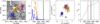 |
Fig. 1 Far left: spatial distribution of clusters from Hunt & Reffert (2023) in the vicinity of Gaia20dsk (shown with a star), overlaid on the DECaPS dust map (Zucker et al. 2025). The arrows indicate the proper motions of the cluster members. Left center: distance distribution of the cluster members. The thick solid and dashed lines show the dBJ distance of Gaia20dsk and its uncertainties. Right center: proper motion distribution of the cluster members and Gaia20dsk, shown with error bars. Far right: Cumulative reddening as a function of distance toward Gaia20dsk, based on the data from Zucker et al. (2025). The red dash-dotted line indicates the most likely distance to Gaia20dsk, while the black solid and dashed lines represent dBJ and its uncertainties. |
2 Properties of Gaia20dsk
2.1 Location and distance
The coordinates of Gaia20dsk are αJ 2000=17h 20m 20.13s and δJ 2000=−35° 48′ 17.78′′, placing it within NGC6334 (see left panel of Fig. 1), which is a well-known star-forming region (Persi & Tapia 2008). Gaia20dsk shares a similar proper motion in right ascension with other members of the group, but with a significantly larger proper motion in declination (see the third panel from the left of Fig. 1), suggesting that it is not a close member of this cluster.
To constrain the distance to Gaia20dsk, we used the 3D DECaPS dust map (Zucker et al. 2025). The cumulative extinction along the line of sight shows a steep rise near 1700 pc (see the last panel of Fig. 1), which is consistent with the NGC6334 cluster distance of  (Hunt & Reffert 2023). Additionally, Bailer-Jones et al. (2021) reported a distance to Gaia20dsk of
  . The estimate relies on photogeometric methods, utilizing Gaia parallax measurements along with Gaia G magnitude and GBP−GRP color data from Gaia EDR3. Owing to the embedded nature of YSOs, the use of the parallax of a single object to estimate its distance is highly uncertain. In the following, we describe how we used both the distance to NGC 6334 (dNGC) from Hunt & Reffert (2023) and the Bailer-Jones et al. (2021) distance (dBJ) to calculate the physical parameters of Gaia20dsk and its accretion.
2.2 Light curve
The multiband light curve of the Gaia20dsk is shown in Fig. 2. The quiescent magnitude of the star is G ∼ 19 mag. Gaia20dsk began brightening in 2019 October and continued brightening for approximately one-and-a-half years before reaching a peak brightness level of 17.2 mag (Δ G=1.8 mag). Gaia20dsk remained at that level until late 2021, when it began to dim. In 2022, the Gaia photometry showed a few bright points, suggesting another brightening event. Starting in 2023 February, the source brightened for the third time at a much faster rate than during the previous episodes and reached a peak of 17.4 mag. For the Gaia measurements, we calculated the uncertainties using the empirical method first presented in Kruszyńska et al. (2022).
We complemented our Gaia light curve with data from the Asteroid Terrestrial-impact Last Alert System (ATLAS; Tonry et al. 2018), utilizing reduced photometry from the ATLAS Forced Photometry server (Shingles et al. 2021). ATLAS has data in two photometric bands: o(λeff=662.98 nm) and c (λeff=518.24 nm). Gaia20dsk was only detected in the o band. To ensure that we used only high-quality photometry, we applied selection criteria based on the chi/N value (as reported by the ATLAS pipeline, which reflects the reduced χ2 from the point spread function (PSF), fitting of individual measurements), signal-to-noise ratio (S/N), and the width at half maximum (FWHM) of the PSF fit. Details of this filtering process are provided in Appendix A. After refining the dataset, we computed weekly median values to improve the clarity of the light curve. The brightening in the o band was confirmed after a careful visual inspection of the target and the surrounding stars. The final o band light curve is shown in Fig. 2. When Gaia20dsk was in quiescence, it was not detected in the o band. A brief brightening event that started in 2022 February (blue triangle in Fig. 2) was observed by ATLAS in the o band, although it was not fully captured by Gaia. The most recent brightening event, which began in early 2023, has remained in a plateau phase since mid-2023.
We constructed the mid-IR (MIR) light curve of Gaia20dsk using NEOWISE (Mainzer et al. 2014) data. Given the relatively large beam size of WISE (FWHMW1=6.1′′, FWHMW2 = 6.4′′), flux contamination from foreground or background sources, or source blending, could affect the measured brightness (Ribas et al. 2014; Dennihy et al. 2020). To assess the potential contamination, we examined higher-resolution images from 2MASS (Skrutskie et al. 2006), Spitzer (Werner et al. 2004), and VIRAC (Smith et al. 2018). We overplotted circles with radii of 1.3 × FWHMW1 and 1.3 × FWHMW2 around the coordinates of Gaia20dsk to simulate the WISE beam size (see Fig. B.1). We defined this search area according to the WISE documentation2. The images revealed a stronger source near our defined search radius; however, the source is not entirely contained within it. Additionally, none of the images underwent an active deblending process, as indicated by the WISE Active deblending quality parameter3. We find that the influence of this source on our data is negligible, and thus no correction was applied (see Appendix B).
After checking the images, we applied filtering based on the quality parameters provided by the NEOWISE-R Single Exposure (L1b) Source Table. The details of this filtering process are provided in Appendix B. Between 2020 August and 2021 March, Gaia20dsk brightened by 0.33 mag in W1 and by 0.5 mag in W2 (see Fig. 2). This event appears to have begun approximately five months after the first G brightening. The brightening event after 2023 was not as clear in the WISE bands as it was in the optical bands. The variability of the WISE light curve is discussed in Sect. 6.
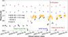 |
Fig. 2 Gaia20dsk light curve. Gaia G photometry is represented by black dots, with error bars similar in size to or smaller than the data points. ATLAS o weekly median photometry is shown in orange. The WISE W1 and W2 bands are represented by blue and red dots, shifted by 9.5 mag for clarity. The dashed vertical line indicates the date of the X-shooter measurements. The three triangles at the bottom of the plot mark the first major burst, which began in 2019 October (green); a short brightening event around 2022 February (blue). A second major burst that started in 2023 February (brown). |
3 Spectroscopic observations
The spectrum of Gaia20dsk was obtained on 2022 June 12 using the X-shooter instrument (Vernet et al. 2011), an echelle spectrograph mounted on the ESO Very Large Telescope at the Paranal Observatory in Chile (Program ID: 108.22LN; PI: Cruz-Sáenz de Miera). By covering the spectral range from 300 to 2500 nm, this instrument can simultaneously observe the ultraviolet (UVB), visible (VIS), and NIR spectra. We used the 0.5′′ × 11′′, 0.4′′ × 11′′, and 0.4′′ × 11′′ size slits, providing spectral resolutions of 9700, 18400, and 11600 in the UVB, VIS, and NIR arms, respectively. The exposure times for UVB, VIS, and NIR regions were 1492 s, 1536 s, and 1600 s, respectively. Gaia20dsk was also measured with the 5′′ × 11′′ slit to correct for slit-losses and estimate the actual flux level by scaling the narrow slit spectrum to match the broad slit spectrum.
The data were reduced using the X-shooter pipeline (Modigliani et al. 2010), and corrected for tellurics using MOLECFIT (Smette et al. 2015; Kausch et al. 2015). The median S/N in the UVB below 556 nm is approximately 0.15, whereas in the VIS range below 750 nm the median S/N is around 2.5. The spectrum (see Fig. 3) shows an increasing flux density toward longer wavelengths and exhibits several emission lines, nine of which are known magnetospheric accretion tracers (Alcalá et al. 2017): Hβ, Hα, the Ca II IR triplet, Paδ, Paγ, Paβ, and Brγ. Hβ and Hα are in the portion of the spectrum with low S/N; therefore, we cannot accurately estimate their line fluxes and caution should be exercised when interpreting them.
3.1 Photosphere of Gaia20dsk: Identification and subtraction
The shape and flux density of emission lines utilized to determine the mass accretion rate are contaminated by the stellar photosphere. The spectral lines flux density and shape are influenced by the continuum level of the star, mostly due to veiling (Hartmann et al. 2016). To eliminate these effects, we subtracted the photospheric contribution from the Gaia20dsk spectrum.
To characterize the photosphere of Gaia20dsk, we compared its spectrum to stellar templates from the third data release of the X-shooter Spectral Library (XSL; Verro et al. 2022), which contains 830 spectra of 683 stars. Because Gaia20dsk is likely a low- to intermediate-mass YSO, we selected template stars with properties characteristic of T Tauri stars (Schiavon et al. 1995) and Herbig Ae/Be stars (Alecian et al. 2013; Montesinos et al. 2009). Specifically, we kept stars with effective temperatures between 4000 and 15 000 K, surface gravities (log g) between 3.0 and 4.5, and metallicities between −0.5 and +0.5. Applying these filters resulted in a subset of 125 XSL templates.
We used a portion of the optical spectrum (8770–8840 Å) of Gaia20dsk to identify its photosphere. This section was chosen because it was the first region containing purely absorption lines (see Fig. 4) and because the effects of veiling are less pronounced at these short wavelengths. The comparison between Gaia20dsk and the 125 templates from the XSL was performed using continuum-normalized spectra. We applied the FIT_CONTINUUM function from the SPECUTILS4 package to the 126 spectra (125 template + Gaia20dsk) in order to determine the continuum level for normalization.
Before finding the best match between Gaia20dsk and the 125 XSL stars, we accounted for the veiling and rotation of accreting stars by applying these effects to each template spectrum. First, we applied a barycentric velocity correction (with the astropy Python package) for the spectral range of Gaia20dsk. The template spectra were then shifted into the same velocity frame as Gaia20dsk, removing relative radial-velocity offsets and enabling a direct comparison of their spectral features. The templates were subsequently broadened by increasing v sin i using the rotBroad function from the PyAstronomy package, which implements rotational broadening following Gray (2005). Broadening was applied over grids of v and i, with v sampled from 0 to 85 km s−1 in steps of 15 km s−1, and i from 0° to 90° in steps of 15°. For each broadening step, we applied a series of veiling factors from 0 to 5 in steps of 0.1, using the following equation,
 (1)
where Ftemp is the continuum-normalized spectrum of the template, vλ is the veiling factor, and
(1)
where Ftemp is the continuum-normalized spectrum of the template, vλ is the veiling factor, and  is the veiled flux density of the continuum-normalized template.
We compared the Gaia20dsk spectrum to each veiled and broadened template, and computed a χ2. Based on the χ2 minimization, two stars emerged as the best fitting templates with the same χ2: HD 116544, and HD 188262. As a final decision, we adopted HD 188262. Using its effective temperature (Teff) together with the derived stellar luminosity of Gaia20dsk yields an age of 0.5−1.4 Myr (see Sect. 5), consistent with the expected evolutionary stage of a Class I or flat spectrum (FS) source (Evans et al. 2009). By contrast, adopting the Teff of HD 116544 implies a much younger age (<0.2 Myr), characteristic of a Class 0 object (Evans et al. 2009). Because Gaia20dsk is classified as a Class I or FS source (see Sect. 4) and its spectrum clearly shows photospheric absorption lines (which are not expected for Class 0 objects). Therefore, we adopted HD 188262 as the preferred template.
The parameters that minimize χ2 for HD 188262 are a veiling factor of vλ=0.1 and broadening factor of v sin i=31 km s−1. HD 188262 has an effective temperature (.Teff) 5919 ± 93 K, with log g being 3.25, while [Fe/H] is 0.27 (Arentsen et al. 2019). We utilized this Teff to determine the stellar parameters in Sect. 5.3. In Fig. 4, we show a portion of the Gaia20dsk spectrum alongside the best-fit template (top panel), the Ca II 8542 Å line before subtraction (middle panel), and the same line after removal of the photospheric component (bottom panel).
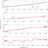 |
Fig. 3 X-shooter spectrum of Gaia20dsk. The optical part is shown in gray, while the IR range is shown in red. The spectrum is not corrected for extinction. The noisy part below 7500 Å is not shown. |
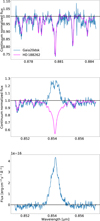 |
Fig. 4 Top panel: segment of the spectra of our target Gaia20dsk (in blue) and the best-fitting photosphere HD 188262 (shown in magenta). See Sect. 3.1 for details. Middle panel: example of one of the Ca II lines before correction with the best-fitting photosphere. The colors indicate the same sources as in the top panel. Bottom panel: photosphere-subtracted accretion-tracing line. |
3.2 Line profiles
The accretion tracer lines include Hβ(λrest=0.486 μm), Hα (λrest=0.656 μm), the Ca II triplet (λrest=0.849 μm, 0.852 μm, 0.866 μm), Paδ(λrest=1.005 μm), Paγ(λrest=1.094 μm), Paβ (λrest=1.282 μm), and Brγ(λrest=2.166 μm). Because veiling is wavelength-dependent, we determined it individually for each spectral line before the photosphere subtraction. For this, we used the photospheric template HD 188262 and the method described in Sect. 3.1. We adopted the v sin i value derived in Sect. 3.1 and we applied Eq. (1) to compute the veiling. In practice, we measured the veiling from the nearby absorption features in the vicinity of each line, while excluding the emission components. On average, the veiling at the end of the VIS range was found to be around vλ ∼ 0.5 (vCaII=0.5 ± 0.1), increasing toward the NIR, reaching vλ ∼ 3.5 (vPa δ=0.5 ± 0.1, vPa γ=2.5 ± 0.1, vPa β=3.5 ± 0.6) in the J band and up to vλ ∼ 10 (νBr γ=10.1 ± 2.5) in the K band.
After photosphere subtraction, most accretion tracer lines show slight blueshift of approximately −10 to −15 km s−1, whereas Ca II triplet lines show slight redshift of about +15 km s−1. These shifts are smaller than the velocity resolution of the spectra (Δ vVIS=16 km s−1, Δ vNIR=26 km s−1) and should therefore be interpreted with caution. In the vicinity of Brγ at 2.167 μm and Hβ at 0.486 μm, we identified a spectral peak that could not be associated with any well-known line. Therefore, we treat it as an artifact and excluded it from further analysis.
Each of the corrected lines exhibits a single-peaked structure (see Figs. in Appendix C). To determine the amplitude, central wavelength, and width of the line profile, we fit Gaussian functions to each of the lines. We fitted a single Gaussian for all lines using the Python CURVE_FIT function, which performs a nonlinear least-squares optimization. In the cases where the line exhibited both broad and narrow components (Ca II triplet, Paδ, Paγ, Paβ, Brγ), we fit two Gaussian components (examples shown in Figs. C.3–C.9). The best-fit values are shown in Table 1.
The combined presence of a broad and narrow component is common in CTTS. The narrow component is thought to originate in the stellar chromosphere, while the broad component is associated with the infalling material (Herbig 2008). For Paδ, we smoothed the spectrum to improve the S/N, as it was noisier than the other lines, complicating the continuum determination. The smoothing was performed by taking the mean flux density over three pixel wide bins.
The two Balmer lines detected in our spectra, Hα and Hβ, both exhibit notably narrow profiles compared to the other emission lines (∼ 250 km s−1. on average). Hβ has a FWHM of 60 ± 1 km s−1 (Fig. C.1), whereas Hα is even narrower, with a FWHM of 47 ± 1 km s−1 (Fig. C.2). The red wing of Hα displays shallow, elongated, and very weak emission features, which might be attributed to outflowing winds.
Among the accretion tracers, the Ca II triplet lines are the strongest emission lines in the NIR spectra (Figs. C.3–C.5). Furthermore, the Ca II 8498 Å line has the narrowest FWHM (231 ± 4 km s−1) among the triplet, while Ca II 8542 Å and Ca II 8662 Å display similar FWHMs (247 ± 2 km s−1. and 253 ± 6 km s−1). Additionally, Ca II 8498 Å is the strongest among the triplet, while Ca II 8662 is the weakest. A similar tendency was previously noted, for example by Hamann & Persson (1992) in their analysis of the Ca II triplet.
In addition to the previous accretion-tracing lines, the spectrum also exhibits several jet-tracing lines, such as [S II] 6716 Å and [S II] 6731 Å, as well as outflow indicators such as [N II] 6548 Å and [N II] 6583 Å (see Figs. C.10–C.13). We note that a double-peaked structure is visible in some forbidden lines, similar to that observed in EX Lupi during its outburst (e.g., Aspin et al. 2010). We detected the He I 10 830 Å (Fig. C.14), which exhibits a broad absorption component that might arise from a stellar wind (e.g., Erkal et al. 2022) or from an outflow (e.g., Kwan & Fischer 2011). The spectrum also shows the H2 21218 Å emission line (see Fig. C.15), which is associated with shocks from molecular outflows (Contreras Peña et al. 2017). We consider these lines to be beyond of the scope of this paper and are not discussed further.
Best-fit parameters of the identified accretion-tracing lines.
4 Spectral energy distribution
We compiled the SED for Gaia20dsk using archival data from the VO SED Analyzer (VOSA) services (Bayo et al. 2008) and VizieR (Ochsenbein et al. 2000). It includes archival photometric data from various surveys, including Gaia (Gaia Collaboration 2023), 2MASS (Skrutskie et al. 2006), WISE (Wright et al. 2010), Spitzer (Werner et al. 2004), DENIS (Epchtein 1994), VIRAC (Smith et al. 2018), and VPHAS+ (Wright 2016). The flux densities used for the SED are listed in Appendix D.
Figure 5 shows the full SED, with different instruments indicated by distinct colors. The X-shooter spectrum is slightly smoothed for clarity, and synthetic photometry was calculated in the I, J, H, and Ks bands to compare with the archival photometric data.
Gaia20dsk shows differences exceeding 3σ between synthetic photometry and archival data in the DENIS I and J bands and the 2MASS J and H bands. In the DENIS J and 2MASS J bands, the source dimmed by 0.24 ± 0.1 mag between 1998 August 10 and October 29, then brightened by 0.29 ± 0.1 mag by 1999 July 22. Without supporting spectroscopy, the significance of these events and whether they are due to changes in accretion or extinction remain unclear.
We applied several photometric methods to classify Gaia20dsk. Using 2MASS and WISE measurements, we computed [H]−[Ks] = 1.24 ± 0.03 mag and [W1]−[W2]=1.32 ± 0.07 mag, suggesting a Class I FS object when compared to Fig. 6 of Koenig & Leisawitz (2014). Spitzer colors [I1] [I2]=0.685 ± 0.07, [I1]−[I3]=1.357 ± 0.04, [I2]− [I3]= 0.672 ± 0.07, and [I2]−[I4] = 1.74 ± 0.07 mag meet the criteria defined by Gutermuth et al. (2008) for a Class II star or slightly earlier. Kuhn et al. (2021) provided three equations for determining the spectral index α (Lada 1987) using NIR photometry between 4 and 24 μm, where interstellar extinction is reduced. Although we lack measurements near 24 μm, we used the Spitzer [I2] – [I4] color and Equation (9) of Kuhn et al. (2021): α[22]−[14] ≈ 1.64 ([I2]−[I4])−2.82. This gives a slope of α[22]−[14]=0.04 ± 0.07, consistent with a FS classification (−0.3 ≤ α<0.3). Considering all three methods, Gaia20dsk has been classified as Class I or FS source.
Objects occupy distinct regions in color-color diagrams and the position of a YSO in the J, H, K space provides insight into its evolutionary stage (see e.g., Lada & Adams 1992). Comparing this position with the extinction vector allows us to assess whether light variation could be caused by extinction. In Fig. 6, the measured J, H, K colors of Gaia20dsk are compared against those of other eruptive young stars: V1647 Ori (Acosta-Pulido et al. 2007), EX Lupi (Juhász et al. 2012), HBC 722 and VSX J205126.1+440523 (Kóspál et al. 2011), V2775 Ori (Caratti o Garatti et al. 2011), and Gaia19bey (Hodapp et al. 2020). Gaia20dsk 2MASS colors are depicted by a red filled circle, while the red star symbol represents the J H Ks synthetic photometry we calculated from the X-shooter spectrum and the open red square represents the VIRAC measurements. We note that to match the VIRAC J, H, Ks data with 2MASS, we applied a color correction for VIRAC bands using the formulas derived by González-Fernández et al. (2018). The cross symbols in the figure indicate the direction of extinction, signifying a measure of 1 magnitude of light attenuation in the V band. The red solid line connecting the 2MASS (filled red circle) and synthetic photometry (red star symbol) data points deviates from the extinction vector; thus, the discrepancy could be attributed to intrinsic variability. In this case, we used RV=3.1 total-to-selective extinction ratio, but using different values (e.g., RV=5.1) does not affect this result. Gaia20dsk shows a similar trend to other sources, as it becomes bluer during bursts, a behavior we discuss in detail in Sect. 6.
In Fig. 7, we present the NEOWISE W1−W2 color curve, which shows Gaia20dsk becoming bluer leading up to the first major brightening event. The star reaches its maximum bluest color at the peak of this brightening event, which occurred between 2020 and 2021. Afterward, the star appears to begin to follow a trend of becoming redder, although this process was interrupted by two events during which the star became bluer. These bluer periods coincide with the brief burst and then the second major burst.
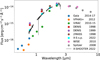 |
Fig. 5 Gaia20dsk SED. Different colored dots denote different surveys, as explained in the legend. The synthetic photometry in I, J, H, and Ks bands represented by the cyan color were computed from the X-shooter spectrum (labeled X-S s.p.). The spectrum itself is plotted with reduced resolution for clarity. The points are not corrected for extinction. The sizes of the error bars are comparable to or smaller than the symbol size. |
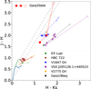 |
Fig. 6 J−H versus H−Ks diagram. The main sequence is represented by a blue thick solid line (Pecaut & Mamajek 2013), the giant branch by a green dashed line (Koornneef 1983), and the reddening path (with AV=1 mag steps) by gray cross symbols (Cardelli et al. 1989). The T Tauri locus is shown as an orange dash-dotted line (Meyer et al. 1997). Open squares denote quiescent colors, while filled squares represent outburst colors. For Gaia20dsk, the filled dot corresponds to the 2MASS measurements from 1998, the filled square to the VIRAC measurements (2010–2015), and the star symbol indicates synthetic photometry derived from the X-shooter spectrum (2020). The error sizes are smaller than or comparable to the symbol sizes. |
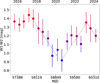 |
Fig. 7 WISE W1−W2 color curve. The panel illustrates how Gaia20dsk became bluer approaching the first major brightening event. Following this, two episodes of blueward color changes occur, superimposed on an overall reddening trend, which coincide with the brief and second major bursts. |
5 Analysis
In this section, the stellar parameters of Gaia20dsk (e.g., luminosity, radius, age, and mass) as well as its accretion properties (e.g., accretion luminosity and accretion rate) are reported. For outbursting young stars, photometric data suggest an accretion outburst, but do not provide a confirmation. To confirm these outbursts, it is necessary to estimate the mass accretion rate during the bright phases of the event and compare it to an accretion rate measured during quiescence (if possible) or to a standard quiescent mass accretion rate. To calculate the mass accretion rate (Macc), we first need to estimate the accretion luminosity (Lacc). We applied two methods to determine this: one based on the integration of the SED and the other on empirical relationships between the accretion luminosity and the luminosity of accretion tracer spectral lines.
5.1 Accretion luminosities from the SED
As a first approach, we used the quiescence and the burst SEDs to estimate  . Given that our source is classified as Class I or FS, the bolometric luminosity in quiescence,
  , arises from multiple components: the stellar photosphere, the accretion luminosity (which persists even during quiescence), and the surrounding circumstellar material, including the disk and envelope. During a burst, we assume the bolometric luminosity,
  , can be expressed as the sum of this quiescent luminosity and an additional accretion luminosity component,
  , resulting from enhanced accretion,
 (2)
(2)
The burst SED was compiled using synthetic photometry, while the quiescent SED was constructed from VIRAC measurements. In both cases, WISE and Spitzer data were used for wavelengths beyond the K band, assuming that the SED shape remained unchanged at these longer wavelengths. This assumption was supported by the fact that the K-band photometry remained largely unchanged between burst and quiescence. Bolometric luminosities were estimated by fitting the data points with a spline function and integrating in the log λ−log Fλ plane. The longest available wavelength is 8 μm from Spitzer. Beyond this, we assumed the flux declines as 1/λ2 and we extrapolated the SED out to 100 μm. These bolometric luminosities should be considered lower limits because the lack of long-wavelength coverage may underestimate emission from possible colder material. Before integrating, we corrected for foreground extinction using interstellar AV values from the DECaPS dust map (Zucker et al. 2025). We did not correct for local extinction because that surrounding material re-radiates absorbed energy at longer wavelengths. Afterward, we integrated the SED and computed the bolometric luminosity using Lbol=4πd2F, where d is the distance, and F is the integrated flux.
Based on the calculations and assuming  , the bolometric luminosity increased from 92 to 100 L⊙ as a result of the burst. Similarly, assuming
  , it increased from 231 to 257 L⊙. These changes correspond to accretion luminosities of 8 and 26 L⊙, respectively. The calculated bolometric and accretion luminosities, as well as the AV values used, are listed in Table 2.
Calculated accretion properties based on the SED and derived stellar parameters.
Accretion-tracing lines used to determine Lacc and Macc.
5.2 Accretion luminosities from empirical relationships
To compare the  values computed in the previous subsection, we derived accretion luminosities under the assumption that mass is delivered onto the star via magnetospheric accretion. We measured the line fluxes, fline, of four accretion-tracing lines: Paδ, Paγ, Paβ, and Brγ, using the line_flux function from the specutils Python package. In these calculations we did not use the Hα, Hβ due to their potential contamination by non-accretion-related processes such as outflows. Additionally, we excluded the Ca II triplet lines (8498 Å, 8542 Å, 8662 Å) following the Alcalá et al. (2017) and Fairlamb et al. (2017) recommendations, as these lines are less reliable for deriving Lacc. The line luminosities were then calculated as Lline = 4πd2 fline, where d is the distance to the star and fline is the extinction-corrected flux.
The accretion luminosities were derived from Lline using empirical relationships of the form
 (3)
where the coefficients a and b were adopted from Alcalá et al. (2017) and Fairlamb et al. (2017), who calibrated these relations for low-mass and intermediate-mass protostars, respectively.
(3)
where the coefficients a and b were adopted from Alcalá et al. (2017) and Fairlamb et al. (2017), who calibrated these relations for low-mass and intermediate-mass protostars, respectively.
Before applying these relations, we corrected the line fluxes not only for foreground extinction, but also for local extinction toward Gaia20dsk. As no extinction value was previously reported for this source, we used the accretion luminosities to estimate AV toward Gaia20dsk. In the absence of extinction (AV=0 mag), all accretion-tracing lines are expected to yield the same Lacc. Thus, we computed Lacc without extinction correction and searched for the value of AV for which the corrected line luminosities produced consistent accretion luminosities across the different tracers. Extinction corrections were performed using the Cardelli et al. (1989) reddening law with RV=3.1, implemented via the CCM89 routine from the dust_extinction Python package. Our estimated extinction is AV=8.6 ± 1.7 mag, which we used during the calculations. Since the distance acts as a uniform scaling factor applied equally to all line luminosities, the two distance estimates yielded the same extinction value. We found that the derived AV is consistent regardless of whether the Alcalá et al. (2017) or Fairlamb et al. (2017) coefficients are used to compute Lacc.
In addition, we estimated the visual extinction by projecting the source position from the 2020 measurements in the J−H vs. H−Ks color–color diagram (red star in Fig. 6) onto the locus of unreddened CTTS (Meyer et al. 1997) along the reddening vector using the extinction law of Cardelli et al. (1989). This gave AV=8.9 ± 1.9 mag, consistent with the values obtained from the empirical relations. The measured line fluxes, line luminosities, and accretion luminosities for each tracer are listed in Table 3.
5.3 Stellar parameters and mass accretion rate
To obtain accurate estimates of Macc, we first need to constrain the stellar parameters, including stellar luminosity. The stellar luminosities were estimated following the method of Fiorellino et al. (2021), which uses the K band photometry and bolometric correction to estimate the stellar luminosity. Because Gaia20dsk is a Class I source, its observed flux contains contributions from both the star and the circumstellar disk and envelope. To account for this excess, we included the K band veiling parameter, rK, in the calculation. This veiling was determined following the method described in Sect. 3.1, adopting the v sin i value derived in Sect. 3.1 and using the spectral region around the Brγ line (2.162–2.172 μm), excluding the emission component itself. The result is rK=10.1 ± 2.5. We computed the bolometric magnitude as
 (4)
where BCK is the bolometric correction, mK is the brightness, rK is the veiling, AK is the extinction, and d is the distance (K in the subscript denotes quantities measured in the K band). We adopted BCK=1.33 ± 0.03 mag from Pecaut & Mamajek (2013), corresponding to the effective temperature of Teff=5919 ± 93 K derived from our analysis (see Sect. 3.1). For the other parameters, we used mK=8.73 ± 0.01 mag from synthetic photometry and AK=1.0 ± 0.2 mag. We converted the AV values from Sect. 5.2 to K band extinction using the Cardelli et al. (1989) law. With these values, we obtained Mbol=−0.35 ± 0.65 mag and 0.58 ± 0.32 mag for the two distance estimates, dBJ and dNGC, respectively.
(4)
where BCK is the bolometric correction, mK is the brightness, rK is the veiling, AK is the extinction, and d is the distance (K in the subscript denotes quantities measured in the K band). We adopted BCK=1.33 ± 0.03 mag from Pecaut & Mamajek (2013), corresponding to the effective temperature of Teff=5919 ± 93 K derived from our analysis (see Sect. 3.1). For the other parameters, we used mK=8.73 ± 0.01 mag from synthetic photometry and AK=1.0 ± 0.2 mag. We converted the AV values from Sect. 5.2 to K band extinction using the Cardelli et al. (1989) law. With these values, we obtained Mbol=−0.35 ± 0.65 mag and 0.58 ± 0.32 mag for the two distance estimates, dBJ and dNGC, respectively.
From the bolometric magnitude, we derive the stellar luminosity using
 (5)
where Mbol, ⊙=4.74 mag is the solar bolometric luminosity. The resulting luminosities are approximately 110 L⊙ for dBJ and 45 L⊙ for dNGC. The exact numbers are presented in Table 2. The stellar parameters were derived using the online tool provided by Lionel Siess5, which implements the pre-main sequence evolutionary models of Siess et al. (2000).
(5)
where Mbol, ⊙=4.74 mag is the solar bolometric luminosity. The resulting luminosities are approximately 110 L⊙ for dBJ and 45 L⊙ for dNGC. The exact numbers are presented in Table 2. The stellar parameters were derived using the online tool provided by Lionel Siess5, which implements the pre-main sequence evolutionary models of Siess et al. (2000).
We assumed a metallicity of Z=0.02, but using different metallicity values did not significantly affect the results. This method provides estimates for the stellar mass and radius, yielding M*=3.2−4.3 M⊙ and R*=6−9.7 R⊙, depending on the assumed distances.
Finally, using the stellar parameters and the accretion luminosities derived earlier from the empirical relationships and from the SED, we computed the mass accretion rate with the standard magnetospheric accretion formula
 (6)
where G is the gravitational constant and the factor 1.25 assumes an inner disk truncation radius Rin=5 R* (Hartmann et al. 2016).
(6)
where G is the gravitational constant and the factor 1.25 assumes an inner disk truncation radius Rin=5 R* (Hartmann et al. 2016).
Figure E.1 shows the extinction-corrected Ṁacc for both distance estimates and both relationships. Table 2 presents the rates based on the SED and presents the stellar properties and Table 3 lists the rates derived from individual tracers.
6 Discussion
The results from Sects. 5.2 and 5.3 are presented in Fig. 8. Points labeled Alcalá et al. (2017) and Fairlamb et al. (2017) show the average Lacc and Macc from accretion-tracing lines (see Sect. 5.2). The results for each line used in the averaging are in Table 3. Overall, the Lacc and Macc values derived from the SED are consistent with those from the empirical relationships, supporting the conclusion that the observed brightening resulted from enhanced accretion. We note that spectroscopic follow-up, including a quiescent spectrum and a corresponding quiescent Macc determination, would provide an independent check. This would further support the observed changes in accretion.
Eruptive YSOs show a range of characteristics, but comparisons with similar objects help place Gaia20dsk in context. Gaia19bey, a MNor, is one such object, sharing characteristics with Gaia20dsk (Hodapp et al. 2020). Both sources are embedded YSOs with similar classifications, namely: Gaia19bey is a Flat-spectrum source, while Gaia20dsk falls into the Class I or FS category. In terms of spectroscopic features, both objects exhibit strong H i emission lines along with a prominent Ca II IR triplet. Molecular hydrogen emission is also present in both spectra. Additionally, they occupy a similar region and exhibit comparable variations in the J−H versus H−Ks color–color diagram (see Fig. 6). During its 2019 outburst, Gaia19bey exhibited an accretion rate of  . The mass accretion rates derived for Gaia20dsk are comparable, with
  for dNGC and
  for dBJ.
Prior to late 2019, the star exhibited no changes in brightness since 2015, when the first Gaia measurements were taken. However, since then, Gaia20dsk has experienced two major burst events and one brief burst. During the first major burst, Gaia20dsk brightened by about 1.8 magnitudes in the G band, with a rate of 0.15 magnitudes per month for approximately one-and-a-half years, and the entire burst event lasted for two years. After the first burst, Gaia20dsk did not return to its previous brightness state. It is possible that the enhanced accretion rate did not revert to the quiescent stage, but only decreased. The duration of Gaia20dsk’s first major burst, of approximately two years, aligns with MNor-type variability timescales, namely, of >1.5 years (Contreras Peña et al. 2017).
The WISE light curve shows only weak variability, with changes less pronounced than those seen in the optical bands. Our data do not allow firm conclusions regarding the origin of this behavior in Gaia20dsk. What we can conclude is that the WISE photometry of Gaia20dsk is not significantly affected by contamination from nearby sources, and that the NIR changes are not attributable to variable extinction, as supported by our color-color diagram analysis. Similar cases of weak NIR variability compared to the optical have been reported in other eruptive YSOs, such as Gaia18cjb, a Class I object (Fiorellino et al. 2024), and EX Lupi during its 2022 outburst (Cruz-Sáenz de Miera et al. 2023). However, the physical origin of such weak IR responses may differ from source to source.
The NIR color light curve and color-color diagram show that Gaia20dsk became bluer during its burst events. This behavior is typical for young stars experiencing outbursts, as they often become bluer, shifting their position toward the T Tauri locus in the diagram (e.g., Lorenzetti et al. 2012; Hodapp et al. 2019). The changes observed in Gaia20dsk are similar to those seen in other well-known young eruptive stars, such as V1647 Ori (e.g., Mosoni et al. 2013), Gaia19bey (Hodapp et al. 2020) and V2775 Ori (Caratti o Garatti et al. 2011). Based on the VIRAC and 2MASS photometry, we conclude that the brightening observed in 1998 was a real physical event and not the result of changing extinction. This is supported by the fact that the observed variations do not follow the extinction path and show a bluer trend similar to that seen during the outburst of V2775 Ori (see Fig. 6). Additionally, Gaia20dsk’s 1998 flux densities (2MASS) were significantly higher than in 2020 (synthetic photometry), exceeding the 3σ level and indicating a stronger burst 22 years earlier.
The spectrum reveals a prominent Hα emission along with the [S II] lines at 6716 Å and 6731 Å. These features, taken together, typically indicate the presence of Herbig-Haro shocks (Hodapp et al. 2020). Furthermore, the Ca II triplet lines are the strongest among the IR lines, a characteristic commonly observed in T Tauri stars (e.g., Muzerolle et al. 1998). Under optically thin conditions, the expected intensity ratio of these three Ca II lines is approximately 1: 9: 5, as reported by Azevedo et al. (2006) for CTTS. In the case of Gaia20dsk, however, the observed ratio approaches unity, suggesting that the emission originates from a region that is a nearly optically thick. This behavior parallels that seen in Gaia19bey, which has been identified as a MNor. Notably, this star also displayed combined Hα and [S II] emission features. Our spectrum also exhibits emission from H2 at 2.12 μm, which is associated with shocks caused by molecular outflows connected to the outburst event, which is an important characteristic of MNors (Contreras Peña et al. 2017).
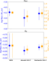 |
Fig. 8 Lacc and Macc based on SED, Alcalá et al. (2017) relationship, and on Fairlamb et al. (2017) relationship. The orange squares show the Lacc, while the blue dots show the corresponding Macc. The presented accretion properties from the two aforementioned relationships are the mean values of the individual measurements of each accretion tracer line summarized in Table 3. |
7 Conclusion
Our analysis of photometric and spectroscopic data indicates that Gaia20dsk has undergone an accretion outburst. Its properties do not clearly correspond to classical EXor or FUor categories; we propose that Gaia20dsk represents an intermediate case resembling that of MNors. Following the criteria defined by Contreras Peña et al. (2017) for this subclass, we compared Gaia20dsk’s characteristics to these standards:
- 1
SEDs corresponding to Class I or FS sources, which Gaia20dsk also satisfies (see Sect. 4).
- 2
Outburst durations lasting longer than 1.5 years, but shorter than those of FUors. Gaia20dsk meets this criterion, with its first major burst lasting over two years (see Fig. 2).
- 3
Spectroscopic features typical of eruptive variables. This is also true for Gaia20dsk, which shows accretion tracer lines common in outbursting YSOs (see Sect. 3.2). Although CO emission is absent, this does not contradict its classification, as CO lines may be suppressed by strong veiling or envelope emission (Contreras Peña et al. 2017).
- 4
MNors typically exhibit H2 emission at 2.122 μm. This emission line is detected in our spectrum as well (see Fig. C.15).
Furthermore, while it was not set as a formal criterion, Contreras Peña et al. (2017) found that MNors usually have a bolometric luminosity approximately one order of magnitude greater than their accretion luminosity. This feature is also observed in Gaia20dsk, where this ratio is roughly 0.1. In addition, another characteristic of MNors is that they have a high bolometric luminosity in the range of hundreds to thousands of L⊙, which holds for Gaia20dsk in the case of dB J distance (∼ 230−260 L⊙) and close to this limit in dNGC distance (∼ 90−100 L⊙).
Considering these criteria and the fact that our source shows similarities with such objects as V1647 Ori, Gaia19bey, and Gaia18cjb (three stars known to be intermediate between EXors and FUors), we conclude that Gaia20dsk is a member of the MNor-type YSos.
Acknowledgements
I dedicate this work to the memory of my beloved mother, Ibolya Nődl, whose love, guidance, and encouragement continue to inspire me. She was the one I loved the most, and her love, supports remain in my heart always. We wish to thank the referee for a careful reading of this paper and for several major comments that significantly improved the conclusions. Fernando Cruz-Sáenz de Miera received financial support from the European Research Council (ERC) under the European Union’s Horizon 2020 research and innovation programme (ERC Starting Grant “Chemtrip”, grant agreement No. 949278). Z.N. was supported by the János Bolyai Research Scholarship of the Hungarian Academy of Sciences. Eleonora Fiorellino has been partially supported by project AYA2018-RTI-096188-B-I00 from the Spanish Agencia Estatal de Investigación and by Grant Agreement 101004719 of the EU project ORP. We acknowledge the Hungarian National Research, Development and Innovation Office grant OTKA FK 146023. This work was also supported by the NKFIH NKKP grant ADVANCED 149943 and the NKFIH excellence grant TKP2021-NKTA-64. Project no. 149943 has been implemented with the support provided by the Ministry of Culture and Innovation of Hungary from the National Research, Development and Innovation Fund, financed under the NKKP ADVANCED funding scheme. We acknowledge support from the ESA PRODEX contract no. 4000132054. Zsófia M. Szabó acknowledges funding from a St. Leonards scholarship from the University of St. Andrews. Zsófia M. Szabó of the International Max Planck Research School (IMPRS) for Astronomy and Astrophysics at the Universities of Bonn and Cologne. Lukasz Wyrzykowski acknowledges Polish National Science Centre grant DAINA 2024/52/L/ST9/00210 and the European Union’s Horizon Europe Research and Innovation programme ACME grant No. 101131928. This publication makes use of VOSA, developed under the Spanish Virtual Observatory project funded by MCIN/AEI/10.13039/501100011033/ through grant PID2020-112949GB-I00. This work has made use of data from the Asteroid Terrestrial-impact Last Alert System project primarily funded to search for near earth asteroids through NASA grants NN12AR55G, 80NSSC18K0284, and 80NSSC18K1575. This research has made use of the NASA/IPAC Infrared Science Archive, which is funded by the National Aeronautics and Space Administration and operated by the California Institute of Technology. We acknowledge ESA Gaia, DPAC and the Photometric Science Alerts Team. This publication makes use of data products from the Near-Earth Object Wide-field Infrared Survey Explorer. It is funded by the National Aeronautics and Space Administration. This research has made use of the SIMBAD database, operated at CDS, Strasbourg, France. This research has made use of the VizieR catalogue access tool, CDS, Strasbourg, France.
References
- Acosta-Pulido, J. A., Kun, M., Ábrahám, P., et al. 2007, AJ, 133, 2020 [NASA ADS] [CrossRef] [Google Scholar]
- Alcalá, J. M., Natta, A., Manara, C. F., et al. 2014, A&A, 561, A2 [NASA ADS] [CrossRef] [EDP Sciences] [Google Scholar]
- Alcalá, J. M., Manara, C. F., Natta, A., et al. 2017, A&A, 600, A20 [NASA ADS] [CrossRef] [EDP Sciences] [Google Scholar]
- Alecian, E., Wade, G. A., Catala, C., et al. 2013, MNRAS, 429, 1001 [NASA ADS] [CrossRef] [Google Scholar]
- Antoniucci, S., Giannini, T., Li Causi, G., & Lorenzetti, D., 2014, ApJ, 782, 51 [Google Scholar]
- Arentsen, A., Prugniel, P., Gonneau, A., et al. 2019, VizieR Online Data Catalog: XSL atmospheric parameters (Arentsen+, 2019), VizieR On-line Data Catalog: J/A+A/627/A138. Originally published in: 2019A&A...627A.138A [Google Scholar]
- Aspin, C., & Reipurth, B., 2009, AJ, 138, 1137 [NASA ADS] [CrossRef] [Google Scholar]
- Aspin, C., Reipurth, B., Herczeg, G. J., & Capak, P., 2010, ApJ, 719, L50 [NASA ADS] [CrossRef] [Google Scholar]
- Audard, M., Ábrahám, P., Dunham, M. M., et al. 2014, in Protostars and Planets VI, eds. H. Beuther, R. S. Klessen, C. P. Dullemond, & T. Henning, 387 [Google Scholar]
- Azevedo, R., Calvet, N., Hartmann, L., et al. 2006, A&A, 456, 225 [NASA ADS] [CrossRef] [EDP Sciences] [Google Scholar]
- Bailer-Jones, C. A. L., Rybizki, J., Fouesneau, M., Demleitner, M., & Andrae, R., 2021, VizieR Online Data Catalog: Distances to 1.47 billion stars in Gaia EDR3 (Bailer-Jones+, 2021), VizieR On-line Data Catalog: I/352. Originally published in: 2021AJ....161..147B [Google Scholar]
- Bayo, A., Rodrigo, C., Barrado Y Navascués, D., et al. 2008, A&A, 492, 277 [NASA ADS] [CrossRef] [EDP Sciences] [Google Scholar]
- Caratti o Garatti, A., Garcia Lopez, R., Scholz, A., et al. 2011, A&A, 526, L1 [NASA ADS] [CrossRef] [EDP Sciences] [Google Scholar]
- Cardelli, J. A., Clayton, G. C., & Mathis, J. S., 1989, ApJ, 345, 245 [Google Scholar]
- Carpenter, J. M., Hillenbrand, L. A., & Skrutskie, M. F., 2001, AJ, 121, 3160 [NASA ADS] [CrossRef] [Google Scholar]
- Cody, A. M., Stauffer, J., Baglin, A., et al. 2014, AJ, 147, 82 [Google Scholar]
- Connelley, M. S., & Reipurth, B., 2018, ApJ, 861, 145 [NASA ADS] [CrossRef] [Google Scholar]
- Contreras Peña, C., Lucas, P. W., Kurtev, R., et al. 2017, MNRAS, 465, 3039 [Google Scholar]
- Cruz-Sáenz de Miera, F., Kóspál, Á., Ábrahám, P., et al. 2022, ApJ, 927, 125 [CrossRef] [Google Scholar]
- Cruz-Sáenz de Miera, F., Kóspál, Á., Abrahám, P., et al. 2023, A&A, 678, A88 [NASA ADS] [CrossRef] [EDP Sciences] [Google Scholar]
- Dennihy, E., Farihi, J., Gentile Fusillo, N. P., & Debes, J. H., 2020, ApJ, 891, 97 [CrossRef] [Google Scholar]
- Epchtein, N. 1994, Exp. Astron., 3, 73 [Google Scholar]
- Erkal, J., Manara, C. F., Schneider, P. C., et al. 2022, A&A, 666, A188 [NASA ADS] [CrossRef] [EDP Sciences] [Google Scholar]
- Evans II, N. J., Dunham, M. M., Jørgensen, J. K., et al. 2009, ApJS, 181, 321 [NASA ADS] [CrossRef] [Google Scholar]
- Fairlamb, J. R., Oudmaijer, R. D., Mendigutia, I., Ilee, J. D., & van den Ancker, M. E., 2017, MNRAS, 464, 4721 [NASA ADS] [CrossRef] [Google Scholar]
- Fiorellino, E., Manara, C. F., Nisini, B., et al. 2021, A&A, 650, A43 [NASA ADS] [CrossRef] [EDP Sciences] [Google Scholar]
- Fiorellino, E., Ábrahám, P., Kóspál, Á., et al. 2024, A&A, 686, A160 [NASA ADS] [CrossRef] [EDP Sciences] [Google Scholar]
- Fischer, W. J., Hillenbrand, L. A., Herczeg, G. J., et al. 2023, in Astronomical Society of the Pacific Conference Series, 534, Protostars and Planets VII, eds. S. Inutsuka, Y. Aikawa, T. Muto, K. Tomida, & M. Tamura, 355 [Google Scholar]
- Gaia Collaboration (Vallenari, A., et al.,) 2023, A&A, 674, A1 [NASA ADS] [CrossRef] [EDP Sciences] [Google Scholar]
- Giannini, T., Schisano, E., Nisini, B., et al. 2024, ApJ, 967, 41 [Google Scholar]
- González-Fernández, C., Hodgkin, S. T., Irwin, M. J., et al. 2018, MNRAS, 474, 5459 [Google Scholar]
- Gray, D. F., 2005, The Observation and Analysis of Stellar Photospheres [Google Scholar]
- Gutermuth, R. A., Myers, P. C., Megeath, S. T., et al. 2008, ApJ, 674, 336 [NASA ADS] [CrossRef] [Google Scholar]
- Hamann, F., & Persson, S. E., 1992, ApJS, 82, 247 [NASA ADS] [CrossRef] [Google Scholar]
- Hartmann, L., & Kenyon, S. J., 1996, ARA&A, 34, 207 [Google Scholar]
- Hartmann, L., Herczeg, G., & Calvet, N., 2016, ARA&A, 54, 135 [Google Scholar]
- Herbig, G. H., 1977, ApJ, 217, 693 [NASA ADS] [CrossRef] [Google Scholar]
- Herbig, G. H., 2008, AJ, 135, 637 [Google Scholar]
- Herbst, W., Herbst, D. K., Grossman, E. J., & Weinstein, D., 1994, AJ, 108, 1906 [Google Scholar]
- Hillenbrand, L. A., Miller, A. A., Carpenter, J. M., et al. 2019, ApJ, 874, 82 [NASA ADS] [Google Scholar]
- Hodapp, K. W., Reipurth, B., Pettersson, B., et al. 2019, AJ, 158, 241 [NASA ADS] [CrossRef] [Google Scholar]
- Hodapp, K. W., Denneau, L., Tucker, M., et al. 2020, AJ, 160, 164 [NASA ADS] [CrossRef] [Google Scholar]
- Hodgkin, S. T., Harrison, D. L., Breedt, E., et al. 2021, A&A, 652, A76 [NASA ADS] [CrossRef] [EDP Sciences] [Google Scholar]
- Hunt, E. L., & Reffert, S., 2023, A&A, 673, A114 [NASA ADS] [CrossRef] [EDP Sciences] [Google Scholar]
- Juhász, A., Dullemond, C. P., van Boekel, R., et al. 2012, ApJ, 744, 118 [Google Scholar]
- Jurdana-Šepić, R., Munari, U., Antoniucci, S., Giannini, T., & Lorenzetti, D., 2018, A&A, 614, A9 [NASA ADS] [CrossRef] [EDP Sciences] [Google Scholar]
- Kausch, W., Noll, S., Smette, A., et al. 2015, A&A, 576, A78 [NASA ADS] [CrossRef] [EDP Sciences] [Google Scholar]
- Koenig, X. P., & Leisawitz, D. T., 2014, ApJ, 791, 131 [Google Scholar]
- Koornneef, J., 1983, A&A, 128, 84 [NASA ADS] [Google Scholar]
- Kóspál, Á., Ábrahám, P., Acosta-Pulido, J. A., et al. 2011, A&A, 527, A133 [NASA ADS] [CrossRef] [EDP Sciences] [Google Scholar]
- Kóspál, Á., Ábrahám, P., Acosta-Pulido, J. A., et al. 2012, ApJS, 201, 11 [CrossRef] [Google Scholar]
- Kruszyńska, K., Wyrzykowski, Ł., Rybicki, K. A., et al. 2022, A&A, 662, A59 [NASA ADS] [CrossRef] [EDP Sciences] [Google Scholar]
- Kuhn, M. A., de Souza, R. S., Krone-Martins, A., et al. 2021, ApJS, 254, 33 [NASA ADS] [CrossRef] [Google Scholar]
- Kwan, J., & Fischer, W., 2011, MNRAS, 411, 2383 [Google Scholar]
- Lada, C. J., 1987, in Star Forming Regions, 115, eds. M. Peimbert, & J. Jugaku, 1 [NASA ADS] [Google Scholar]
- Lada, C. J., & Adams, F. C., 1992, ApJ, 393, 278 [Google Scholar]
- Liu, H., Herczeg, G. J., Johnstone, D., et al. 2022, ApJ, 936, 152 [NASA ADS] [CrossRef] [Google Scholar]
- Lorenzetti, D., Antoniucci, S., Giannini, T., et al. 2012, ApJ, 749, 188 [NASA ADS] [CrossRef] [Google Scholar]
- Lucas, P. W., Elias, J., Points, S., et al. 2020, MNRAS, 499, 1805 [Google Scholar]
- Mainzer, A., Bauer, J., Cutri, R. M., et al. 2014, ApJ, 792, 30 [Google Scholar]
- Meyer, M. R., Calvet, N., & Hillenbrand, L. A., 1997, AJ, 114, 288 [Google Scholar]
- Modigliani, A., Goldoni, P., Royer, F., et al. 2010, SPIE Conf. Ser., 7737, 773728 [Google Scholar]
- Montesinos, B., Eiroa, C., Mora, A., & Merín, B., 2009, A&A, 495, 901 [NASA ADS] [CrossRef] [EDP Sciences] [Google Scholar]
- Mosoni, L., Sipos, N., Ábrahám, P., et al. 2013, A&A, 552, A62 [NASA ADS] [CrossRef] [EDP Sciences] [Google Scholar]
- Muzerolle, J., Hartmann, L., & Calvet, N., 1998, AJ, 116, 455 [Google Scholar]
- Nagy, Z., Park, S., Ábrahám, P., et al. 2023, MNRAS, 524, 3344 [NASA ADS] [CrossRef] [Google Scholar]
- Ochsenbein, F., Bauer, P., & Marcout, J., 2000, A&AS, 143, 23 [Google Scholar]
- Park, S., Kóspál, Á., Ábrahám, P., et al. 2022, ApJ, 941, 165 [NASA ADS] [CrossRef] [Google Scholar]
- Pecaut, M. J., & Mamajek, E. E., 2013, ApJS, 208, 9 [Google Scholar]
- Persi, P., & Tapia, M., 2008, in Handbook of Star Forming Regions, Volume II, 5, ed. B. Reipurth, 456 [Google Scholar]
- Ribas, Á., Merín, B., Bouy, H., & Maud, L. T. 2014, A&A, 561, A54 [NASA ADS] [CrossRef] [EDP Sciences] [Google Scholar]
- Schiavon, R. P., Batalha, C., & Barbuy, B., 1995, A&A, 301, 840 [Google Scholar]
- Shingles, L., Smith, K. W., Young, D. R., et al. 2021, Transient Name Server AstroNote, 7, 1 [NASA ADS] [Google Scholar]
- Siess, L., Dufour, E., & Forestini, M., 2000, A&A, 358, 593 [Google Scholar]
- Siwak, M., Ogloza, W., Moffat, A. F. J., et al. 2018, MNRAS, 478, 758 [NASA ADS] [CrossRef] [Google Scholar]
- Siwak, M., Hillenbrand, L. A., Kóspál, Á., et al. 2023, MNRAS, 524, 5548 [NASA ADS] [CrossRef] [Google Scholar]
- Siwak, M., Kóspál, Á., Ábrahám, P., et al. 2025, A&A, 695, A130 [NASA ADS] [CrossRef] [EDP Sciences] [Google Scholar]
- Skrutskie, M. F., Cutri, R. M., Stiening, R., et al. 2006, AJ, 131, 1163 [NASA ADS] [CrossRef] [Google Scholar]
- Smette, A., Sana, H., Noll, S., et al. 2015, A&A, 576, A77 [NASA ADS] [CrossRef] [EDP Sciences] [Google Scholar]
- Smith, L. C., Lucas, P. W., Kurtev, R., et al. 2018, MNRAS, 474, 1826 [Google Scholar]
- Szegedi-Elek, E., Ábrahám, P., Wyrzykowski, Ł., et al. 2020, ApJ, 899, 130 [Google Scholar]
- Tonry, J. L., Denneau, L., Heinze, A. N., et al. 2018, PASP, 130, 064505 [Google Scholar]
- Vernet, J., Dekker, H., D’Odorico, S., et al. 2011, A&A, 536, A105 [NASA ADS] [CrossRef] [EDP Sciences] [Google Scholar]
- Verro, K., Trager, S. C., Peletier, R. F., et al. 2022, A&A, 660, A34 [NASA ADS] [CrossRef] [EDP Sciences] [Google Scholar]
- Wenger, M., Ochsenbein, F., Egret, D., et al. 2000, A&AS, 143, 9 [NASA ADS] [Google Scholar]
- Werner, M. W., Roellig, T. L., Low, F. J., et al. 2004, ApJS, 154, 1 [NASA ADS] [CrossRef] [Google Scholar]
- Wright, N. J., 2016, in Astrophysics and Space Science Proceedings, 42, The Universe of Digital Sky Surveys, eds. N. R. Napolitano, G. Longo, M. Marconi, M. Paolillo, & E. Iodice, 55 [Google Scholar]
- Wright, E. L., Eisenhardt, P. R. M., Mainzer, A. K., et al. 2010, AJ, 140, 1868 [Google Scholar]
- Zucker, C., Saydjari, A. K., Speagle, J. S., et al. 2025, ApJ, 992, 39 [Google Scholar]
Appendix A ATLAS data filtering
To select reliable ATLAS photometry, we applied selection criteria based on the χ/N value (which represents the reduced χ2 PSF fitting of individual measurements), the S/N, and the FWHM of the PSF fit. First, we examined the χ/N distribution using histograms (upper panel of Fig. A.1), which was well approximated by a double Gaussian fit. We focused on the narrow Gaussian component, i.e., the peak of the distribution, and set a filtering threshold at μ+3σ, where μ and σ are the mean and standard deviation of the selected Gaussian. Only data points satisfying χ/N<μ+3σ were retained. A similar filtering approach was applied to the FWHM distribution (lower panel of Fig. A.1). Additionally, we retained only measurements with S/N>3.5, calculated using the fluxes and uncertainties in the ATLAS tables. These three selection criteria were combined to refine the dataset before constructing the final light curve.
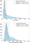 |
Fig. A.1 ATLAS filtering method for the o band. The histograms of χ/N and FWHM were fit with two Gaussian functions. The solid line indicates the mean of the Gaussian closest to the major peak of the distribution. The dashed lines represent this mean value plus/minus the 1σ, 2σ, and 3σ standard deviation. |
Appendix B WISE data analysis
Appendix B.1 Effect of contamination
A nearby source, located to the north of Gaia20dsk and with 2MASS ID 17202041–3548117 (α2000=17h 20m 20.41s, δ2000= −35° 48′ 11.7′′), represents the strongest potential contaminant in the WISE bands. To date, very little is known about this source; a SIMBAD query (Wenger et al. 2000) using a 5′′ search radius returned no results, making it difficult to draw firm conclusions about its nature or behavior. When contemporaneous measurements were available, the contaminating source was fainter by about 2 mag in the J, H, and K bands (based on 2MASS and VIRAC data), and by approximately 3 mag in the Spitzer I1, I2 bands.
Here, the “contamination effect” refers to the fraction of flux in the WISE beam that originates from nearby source. Since no direct WISE measurements are available for the contaminant, we estimated its flux by converting contemporaneous Spitzer measurements into the WISE system using the color transformations of Antoniucci et al. (2014), and then into flux densities using the zeropoints from WISE documentation6.
Assuming total flux measured by WISE is given by
 (B.1)
where FG,Wx and FC,Wx denote the intrinsic fluxes of Gaia20dsk without the contamination and the contaminant, respectively. Using the values from Table D.1, Ftotal,W1=(1.14 ± 0.06) × 10−14 and Ftotal,W2=(1.05 ± 0.07) × 10−14 erg s−1 cm−2 Å−1, and the estimated contaminant fluxes of FC,W1=(6.67 ± 0.31) × 10−16 and FC,W2=(4.80 ± 0.19) × 10−16 erg s−1 cm−2 Å−1, we obtain
(B.1)
where FG,Wx and FC,Wx denote the intrinsic fluxes of Gaia20dsk without the contamination and the contaminant, respectively. Using the values from Table D.1, Ftotal,W1=(1.14 ± 0.06) × 10−14 and Ftotal,W2=(1.05 ± 0.07) × 10−14 erg s−1 cm−2 Å−1, and the estimated contaminant fluxes of FC,W1=(6.67 ± 0.31) × 10−16 and FC,W2=(4.80 ± 0.19) × 10−16 erg s−1 cm−2 Å−1, we obtain


The flux of Gaia20dsk is about 16 and 21 times higher than the contaminant in W 1 and W 2, respectively. The contaminant contribution can also be expressed in magnitude,
 (B.2)
which quantifies by how much the measured Gaia20dsk magnitude would be brightened due to the contaminant. For our data, we find Δ W1 ∼ 0.08 mag and Δ W2 ∼ 0.04 mag. In other words, the presence of the contaminant would increase the observed brightness of Gaia20dsk by at most 0.08 mag in W1 and 0.04 mag in W 2.
(B.2)
which quantifies by how much the measured Gaia20dsk magnitude would be brightened due to the contaminant. For our data, we find Δ W1 ∼ 0.08 mag and Δ W2 ∼ 0.04 mag. In other words, the presence of the contaminant would increase the observed brightness of Gaia20dsk by at most 0.08 mag in W1 and 0.04 mag in W 2.
We found time-series photometry only in ATLAS database. Applying the same filtering method as for Gaia20dsk, we determined that nearly all ATLAS points lie below the detection limit, and inspection of the corresponding images did not reveal the source.
Any potential contamination in the WISE measurements is at most comparable to, or smaller than, the measurement uncertainties, and therefore the contaminant is not expected to significantly affect Gaia20dsk’s observed photometry. Additionally, WISE measures flux using PSF-fitting, which is less susceptible to contamination from nearby sources, and the contaminant only partially overlaps the beam.
Appendix B.2 Data filtering
To select the reliable WISE photometry, we first discarded measurements where the flux was smaller than its uncertainty. Afterward, we filtered out the measurements based on the following criteria: CC_FLAGS is lowercase letter, PH_QUAL is not equal to ‘X’, w1rchi2, and w2rchi2 are less than 50; qI_FACT is nonzero, SAA_SEP is higher than five, MOON_MASKED is not one. The detailed description of these parameters is available from the database website7. Due to the brightening of Gaia20dsk being close to the saturation limits in each band, we applied a correction, which is available on the WISE website8. Finally, we computed the median of multiple exposures of each season.
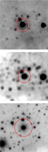 |
Fig. B.1 Images of Gaia20dsk as observed by Spitzer I2 filter (top), 2MASS Ks filter (middle), and VISTA Ks filter (bottom). Circles with radii of 1.3 × FWHMW2 are overplotted to illustrate the WISE beam size. |
Appendix C Line profiles and gaussian fits of accretion tracers
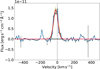 |
Fig. C.1 Extinction-corrected, photosphere-subtracted, and continuum-subtracted line profile of Hβ at 4861 Å. The red curve represents the best fit of the Gaussian(s), while several individual samples showing the range of uncertainties. |
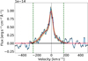 |
Fig. C.6 Similar to Fig. C.1, but for Paδ at 10 049 Å.The green vertical dashed lines indicate the boundaries within which we calculated the line flux. |
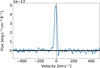 |
Fig. C.10 Extinction-corrected, photosphere-subtracted, continuum-subtracted line profile of [N II] at 6548 Å. |
Appendix D Flux densities used for the SED
Archival and synthetic photometry of Gaia20dsk.
Appendix E Stellar parmeters and accretion properties
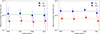 |
Fig. E.1 Mass accretion rate of Gaia20dsk per different accretion-tracing line and considering two different distances. The spectral lines are in order of ascending wavelength. The horizontal green and orange lines show the mean value of the calculated mass accretion rate considering dBJ and dNGC, respectively. The left panel shows the result based on Alcalá et al. (2017) coefficient, while the right panel shows the result based on the Fairlamb et al. (2017) coeeficient. |
All Tables
All Figures
|
Fig. 1 Far left: spatial distribution of clusters from Hunt & Reffert (2023) in the vicinity of Gaia20dsk (shown with a star), overlaid on the DECaPS dust map (Zucker et al. 2025). The arrows indicate the proper motions of the cluster members. Left center: distance distribution of the cluster members. The thick solid and dashed lines show the dBJ distance of Gaia20dsk and its uncertainties. Right center: proper motion distribution of the cluster members and Gaia20dsk, shown with error bars. Far right: Cumulative reddening as a function of distance toward Gaia20dsk, based on the data from Zucker et al. (2025). The red dash-dotted line indicates the most likely distance to Gaia20dsk, while the black solid and dashed lines represent dBJ and its uncertainties. |
| In the text | |
|
Fig. 2 Gaia20dsk light curve. Gaia G photometry is represented by black dots, with error bars similar in size to or smaller than the data points. ATLAS o weekly median photometry is shown in orange. The WISE W1 and W2 bands are represented by blue and red dots, shifted by 9.5 mag for clarity. The dashed vertical line indicates the date of the X-shooter measurements. The three triangles at the bottom of the plot mark the first major burst, which began in 2019 October (green); a short brightening event around 2022 February (blue). A second major burst that started in 2023 February (brown). |
| In the text | |
|
Fig. 3 X-shooter spectrum of Gaia20dsk. The optical part is shown in gray, while the IR range is shown in red. The spectrum is not corrected for extinction. The noisy part below 7500 Å is not shown. |
| In the text | |
|
Fig. 4 Top panel: segment of the spectra of our target Gaia20dsk (in blue) and the best-fitting photosphere HD 188262 (shown in magenta). See Sect. 3.1 for details. Middle panel: example of one of the Ca II lines before correction with the best-fitting photosphere. The colors indicate the same sources as in the top panel. Bottom panel: photosphere-subtracted accretion-tracing line. |
| In the text | |
|
Fig. 5 Gaia20dsk SED. Different colored dots denote different surveys, as explained in the legend. The synthetic photometry in I, J, H, and Ks bands represented by the cyan color were computed from the X-shooter spectrum (labeled X-S s.p.). The spectrum itself is plotted with reduced resolution for clarity. The points are not corrected for extinction. The sizes of the error bars are comparable to or smaller than the symbol size. |
| In the text | |
|
Fig. 6 J−H versus H−Ks diagram. The main sequence is represented by a blue thick solid line (Pecaut & Mamajek 2013), the giant branch by a green dashed line (Koornneef 1983), and the reddening path (with AV=1 mag steps) by gray cross symbols (Cardelli et al. 1989). The T Tauri locus is shown as an orange dash-dotted line (Meyer et al. 1997). Open squares denote quiescent colors, while filled squares represent outburst colors. For Gaia20dsk, the filled dot corresponds to the 2MASS measurements from 1998, the filled square to the VIRAC measurements (2010–2015), and the star symbol indicates synthetic photometry derived from the X-shooter spectrum (2020). The error sizes are smaller than or comparable to the symbol sizes. |
| In the text | |
|
Fig. 7 WISE W1−W2 color curve. The panel illustrates how Gaia20dsk became bluer approaching the first major brightening event. Following this, two episodes of blueward color changes occur, superimposed on an overall reddening trend, which coincide with the brief and second major bursts. |
| In the text | |
|
Fig. 8 Lacc and Macc based on SED, Alcalá et al. (2017) relationship, and on Fairlamb et al. (2017) relationship. The orange squares show the Lacc, while the blue dots show the corresponding Macc. The presented accretion properties from the two aforementioned relationships are the mean values of the individual measurements of each accretion tracer line summarized in Table 3. |
| In the text | |
|
Fig. A.1 ATLAS filtering method for the o band. The histograms of χ/N and FWHM were fit with two Gaussian functions. The solid line indicates the mean of the Gaussian closest to the major peak of the distribution. The dashed lines represent this mean value plus/minus the 1σ, 2σ, and 3σ standard deviation. |
| In the text | |
|
Fig. B.1 Images of Gaia20dsk as observed by Spitzer I2 filter (top), 2MASS Ks filter (middle), and VISTA Ks filter (bottom). Circles with radii of 1.3 × FWHMW2 are overplotted to illustrate the WISE beam size. |
| In the text | |
|
Fig. C.1 Extinction-corrected, photosphere-subtracted, and continuum-subtracted line profile of Hβ at 4861 Å. The red curve represents the best fit of the Gaussian(s), while several individual samples showing the range of uncertainties. |
| In the text | |
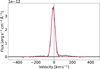 |
Fig. C.2 Same as Fig. C.1, but for Hα at 6563 Å. |
| In the text | |
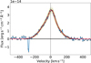 |
Fig. C.3 Same as Fig. C.1, but for Ca II at 8498 Å. |
| In the text | |
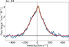 |
Fig. C.4 Same as Fig. C.1, but for Ca II at 8542 Å. |
| In the text | |
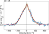 |
Fig. C.5 Same as Fig. C.1, but for Ca II at 8662 Å. |
| In the text | |
|
Fig. C.6 Similar to Fig. C.1, but for Paδ at 10 049 Å.The green vertical dashed lines indicate the boundaries within which we calculated the line flux. |
| In the text | |
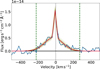 |
Fig. C.7 Same as Fig. C.6, but for Par at 10 938 Å. |
| In the text | |
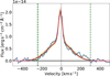 |
Fig. C.8 Same as Fig. C.6, but for Paβ at 12 818 Å. |
| In the text | |
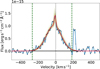 |
Fig. C.9 Same as Fig. C.6, but for Brγ at 21 655 Å. |
| In the text | |
|
Fig. C.10 Extinction-corrected, photosphere-subtracted, continuum-subtracted line profile of [N II] at 6548 Å. |
| In the text | |
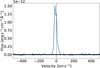 |
Fig. C.11 Same as C.10, but for [N II] at 6583 Å. |
| In the text | |
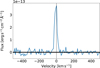 |
Fig. C.12 Same as C.10, but for [S II] at 6716 Å. |
| In the text | |
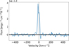 |
Fig. C.13 Same as C.10, but for of [S II] at 6731 Å. |
| In the text | |
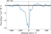 |
Fig. C.14 Same as C.10, but for He I at 10 830 Å. |
| In the text | |
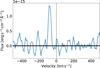 |
Fig. C.15 Same as C.10, but for H2 at 21 218 Å. |
| In the text | |
|
Fig. E.1 Mass accretion rate of Gaia20dsk per different accretion-tracing line and considering two different distances. The spectral lines are in order of ascending wavelength. The horizontal green and orange lines show the mean value of the calculated mass accretion rate considering dBJ and dNGC, respectively. The left panel shows the result based on Alcalá et al. (2017) coefficient, while the right panel shows the result based on the Fairlamb et al. (2017) coeeficient. |
| In the text | |
Current usage metrics show cumulative count of Article Views (full-text article views including HTML views, PDF and ePub downloads, according to the available data) and Abstracts Views on Vision4Press platform.
Data correspond to usage on the plateform after 2015. The current usage metrics is available 48-96 hours after online publication and is updated daily on week days.
Initial download of the metrics may take a while.