| Issue |
A&A
Volume 706, February 2026
|
|
|---|---|---|
| Article Number | A248 | |
| Number of page(s) | 16 | |
| Section | Interstellar and circumstellar matter | |
| DOI | https://doi.org/10.1051/0004-6361/202555924 | |
| Published online | 17 February 2026 | |
Interaction of the central jet with the surrounding gas in the protostellar outflow from IRAS 04166+2706
1
Observatorio Astronómico Nacional (IGN),
Alfonso XII 3,
28014
Madrid,
Spain
2
NRC Herzberg Astronomy and Astrophysics,
5071 West Saanich Rd,
Victoria,
BC
V9E 2E7,
Canada
3
Department of Physics and Astronomy, University of Victoria,
Victoria,
BC
V8P 5C2,
Canada
4
Instituto de Radioastronomía Milimétrica (IRAM),
Av. Divina Pastora 7, Núcleo Central,
18012
Granada,
Spain
5
Center for Astrophysics, Harvard & Smithsonian,
60 Garden Street,
Cambridge,
MA
02138,
USA
6
Institute of Astronomy and Astrophysics, Academia Sinica,
Taipei
106319,
Taiwan
★ Corresponding author: This email address is being protected from spambots. You need JavaScript enabled to view it.
Received:
12
June
2025
Accepted:
20
December
2025
Abstract
Context. The outflow from the Class 0 protostar IRAS 04166+2706 (hereafter IRAS 04166) contains a remarkably symmetric jet-like component of extremely high-velocity (EHV) gas.
Aims. We studied the IRAS 04166 outflow and investigated the relation between its EHV component and the slower outflow gas.
Methods. We mosaicked the CO(2–1) emission from the IRAS 04166 outflow using the 12m and the Compact Arrays of ALMA. We also developed a ballistic toy model of the gas ejected laterally from a jet to interpret the data.
Results. In agreement with previous observations, the ALMA data show that the slow outflow component is distributed in two opposed conical lobes and has a shear-flow pattern with velocity increasing toward the axis. The EHV gas consists of a series of arc-like condensations that span the full width of the conical lobes and merge with their walls, suggesting that the fast and slow outflow components are physically connected. In addition, position–velocity diagrams along the outflow axis show finger-like extensions that connect the EHV emission with the origin of the diagram, as if part of the EHV gas had been decelerated by its interaction with the low-velocity outflow. A ballistic model can reproduce these finger-like extensions assuming that the EHV gas consists of jet material that has been ejected laterally over a short period of time and has transferred part of its momentum to the surrounding shear flow.
Conclusions. The EHV gas in the IRAS 04166 outflow seems to play a role in the acceleration of the slower gas component. The presence of similar finger-like extensions in the position–velocity diagrams of other outflows suggests that this process may be occurring in other systems, even if the EHV component is not seen because it has an atomic composition.
Key words: stars: formation / ISM: jets and outflows / ISM: molecules / radio lines: ISM / ISM: individual objects: IRAS 04166+2706
© The Authors 2026
 Open Access article, published by EDP Sciences, under the terms of the Creative Commons Attribution License (https://creativecommons.org/licenses/by/4.0), which permits unrestricted use, distribution, and reproduction in any medium, provided the original work is properly cited.
This article is published in open access under the Subscribe to Open model. This email address is being protected from spambots. You need JavaScript enabled to view it. to support open access publication.
1 Introduction
Bipolar outflows are ubiquitous in star-forming regions. They are found in protostars of all masses and environments, and seem to represent a necessary ingredient in the process of star formation (see Frank et al. 2014; Bally 2016 for dedicated reviews).
Although they are common and despite multiple decades of research, important aspects of bipolar-outflow physics remain poorly understood. Outflows are thought to be powered by the combined action of gravity, disk rotation, and magnetic fields, but whether the solution to this complex problem results in a wide-angle wind or a highly collimated jet (or some combination of the two) is strongly debated (Raga et al. 1993; Raga & Cabrit 1993; Masson & Chernin 1993; Shu et al. 1994; Shang et al. 2006; Rabenanahary et al. 2022; Shang et al. 2023).
Outflows powered by the youngest protostars often present the highest degree of collimation and the highest velocities, and are thought to best reflect the intrinsic properties of the underlying driving agent (Lee 2020). A subset of these young outflows stands out for the presence of a distinct velocity component that appears in the spectra as a detached secondary peak and is commonly referred to as the extremely high-velocity (EHV) component (e.g., Bachiller 1996). This component presents the highest degree of collimation and often carries a significant fraction of the total outflow energy and momentum, which suggests that it could play a role in the acceleration of the outflow material (Bachiller et al. 1990; Tafalla et al. 2004). The EHV component, in addition, presents an unusual chemical composition rich in SiO and other oxygen-bearing species (Tafalla et al. 2010; Kristensen et al. 2011; Tychoniec et al. 2021) indicative of a different origin from the rest of the outflow, which is likely dominated by swept-up ambient gas. One possibility is that the EHV gas represents a wind from the protostar or the inner disk since its composition resembles that predicted by chemical models (Glassgold et al. 1991; Tabone et al. 2020). Further work is clearly needed to understand the physics and chemistry of the EHV component, and to assess its role in the larger outflow phenomenon.
The outflow from the Class 0 source IRAS 04166+2706 in Taurus (hereafter IRAS 04166), initially discovered by Bontemps et al. (1996), represents an excellent target to investigate the origin and nature of the EHV component. It is at an estimated distance of 156 pc (Krolikowski et al. 2021), and its central source has a luminosity of 0.4 L⊙ and a mass in the range 0.15–0.39 M⊙ (Ohashi et al. 2023; Phuong et al. 2025). No Herbig-Haro objects are associated with it, although Davis et al. (2010) found weak H2 emission along its lobes. Its EHV component was first identified by Tafalla et al. (2004) using the IRAM 30m telescope, and was later studied by Santiago-García et al. (2009) and Wang et al. (2014) using data from the Plateau de Bure Interferometer and the Smithsonian Submillimeter Array. These observations revealed that the EHV component of IRAS 04166 consists of a jet-like chain of condensations that are located symmetrically with respect to the protostar, as if they resulted from a series of episodic ejections. The EHV component, in addition, was found to present a systematic sawtooth velocity pattern in position–velocity (PV) diagrams that resembles those predicted by models of pulsating jets (Stone & Norman 1993, but see Wang et al. 2019 for an alternative interpretation in terms of a wide-angle wind).
Further observations of two selected EHV condensations in the IRAS 04166 outflow were carried out by Tafalla et al. (2017) using the Atacama Large Millimeter/submillimeter Array (ALMA). Analyzing CO(2–1) data, these authors showed that the EHV gas is distributed in parabolic structures reminiscent of bow shocks, and that the material in them is expanding radially with a velocity that increases linearly with distance from the outflow axis. This geometry and kinematics supports the interpretation that the EHV emission represents material that has been ejected laterally from the jet in a series of internal shocks.
To further investigate the EHV component of the IRAS 04166 outflow, we carried out new ALMA observations to map the full length of the main flow and cover multiple EHV peaks. In this paper we present the results of these observations and describe how they provide evidence for physical interaction between the EHV regime and the slower outflow component.
2 Observations
The IRAS 04166 outflow was observed with ALMA using its Band 6 receiver (Ediss et al. 2004; Kerr et al. 2004) between October 2021 and January 2022. The main goal of the project (reference 2021.1.00575.S) was to map the CO(2–1) emission from the outflow, so this line was observed with a bandwidth of 325 km s−1 and a velocity resolution of 0.16 km s−1. Additional correlator windows were used to observe the emission of SiO(5–4), 13CO(2–1), and SO(6,5–5,4) with similar velocity resolutions, and a 2 GHz-wide window was added to observe the continuum emission at a frequency of 232 GHz. Both the ALMA Compact Array (ACA) and the 12m array were used to cover a range of baselines from 8.9 to 976.6m. To map the full extent of the emission, mosaics of 17 and 14 pointings were made with the ACA and 12m arrays, respectively.
The visibilities obtained with the interferometer were calibrated using the CASA software (CASA Team 2022) version 6.2.1-7 and the facility-provided pipeline. After calibration, the continuum ACA and 12m array visibilities were combined and Fourier transformed using the multi frequency synthesis mode and natural weighting for maximum sensitivity. The resulting image was cleaned using the tclean command with the hogbom (Högbom 1974) option and no special mask because the emission was only detected toward the protostar. The beam size was ![Mathematical equation: $\[0^{\prime\prime}_\cdot7 \times 0^{\prime\prime}_\cdot6\]$](/articles/aa/full_html/2026/02/aa55924-25/aa55924-25-eq1.png) , and the image rms noise level was about 60 μJy beam−1.
, and the image rms noise level was about 60 μJy beam−1.
For the spectral-line emission, the calibrated ACA and 12m-array visibilities were resampled to a velocity resolution of 0.5 km s−1, continuum-subtracted using line-free channels, and Fourier-transformed. The resulting maps had a synthesized beam of ![Mathematical equation: $\[0^{\prime\prime}_\cdot7 \times 0^{\prime\prime}_\cdot6\]$](/articles/aa/full_html/2026/02/aa55924-25/aa55924-25-eq2.png) and a typical rms level of 4.4 mJy beam−1 per 0.5 km s−1 channel, equivalent to 0.25 K in brightness temperature. The maps were cleaned with tclean using the multiscale (Cornwell 2008) option (scale sizes of 0, 5, 10, and 20 pixels) and auto-multithresh masking (Kepley et al. 2020). Several tests were carried out to optimize the choice of imaging parameters, although the use of alternative values for the weighting scheme or the cleaning options did not produce significantly different maps.
and a typical rms level of 4.4 mJy beam−1 per 0.5 km s−1 channel, equivalent to 0.25 K in brightness temperature. The maps were cleaned with tclean using the multiscale (Cornwell 2008) option (scale sizes of 0, 5, 10, and 20 pixels) and auto-multithresh masking (Kepley et al. 2020). Several tests were carried out to optimize the choice of imaging parameters, although the use of alternative values for the weighting scheme or the cleaning options did not produce significantly different maps.
Once the images were cleaned using CASA, the data were converted to the GILDAS1 format for further processing. To test the ability of the ALMA observations to recover the outflow emission, we synthesized a series of CO(2–1) spectra assuming an 11″ angular resolution and compared them with the IRAM 30m single-dish observations of Tafalla et al. (2004). This comparison is presented in the left panel of Fig. A.1, and shows that the ALMA observations fully recovered the emission of the EHV outflow regime, which is the main focus of this study. The ALMA observations, however, miss significant emission at velocities lower than about 10 km s−1 with respect to the ambient cloud despite including ACA data, suggesting that the lowest-velocity outflow emission is very extended. As we show, this lowest-velocity extended emission is not critical for the analysis presented here, and if necessary, it can be studied using the lower angular resolution observations of Santiago-García et al. (2009).
3 Results
3.1 Continuum data
The map of the 232 GHz continuum emission only shows a single point-like source toward the position of the protostar, and for completeness is shown in Fig. A.2. While no other emission sources are detected, the map shows a noticeable increase in the level of residuals toward the vicinity of the protostar, which likely results from the interferometer filtering out the extended emission from the dense core that surrounds this Class 0 source. The core has a diameter of about one arcminute, and has been previously mapped at millimeter wavelengths by multiple authors (Motte & André 2001; Tafalla et al. 2004; Hacar et al. 2013; Bracco et al. 2017; Eswaraiah et al. 2021).
To characterize the 232 GHz emission peak we fit it with a 2D Gaussian using the CASA command imfit. The estimated peak flux density is 59.68 ± 0.06 mJy beam−1 at the position ![Mathematical equation: $\[\text{RA(ICRS)=} ~04^{\mathrm{h}} 19^{\mathrm{m}} 42^{\mathrm{s}}_\cdot505, \text{DEC(ICRS)} =27^{\circ} 13^{\prime} 35^{\prime \prime}_\cdot 87\]$](/articles/aa/full_html/2026/02/aa55924-25/aa55924-25-eq3.png) , and the integrated flux is 76.2 ± 0.1 mJy. These values are in good agreement with those derived at approximately the same frequency by Santiago-García et al. (2009) and also by the eDisk ALMA project. These latter observations have an angular resolution ten times higher than ours and reveal a smooth dust disk of approximately 20 au in radius and an inclination of 47° with respect to the line of sight (Ohashi et al. 2023; Phuong et al. 2025). Even at this highest angular resolution, the central source seems to be a single object. Assuming a typical dust temperature of 20 K, optically thin emission, an emissivity per dust mass of 0.9 cm2 g−1 (Ossenkopf & Henning 1994), and a standard gas to dust ratio of 100 (Bohlin et al. 1978), the estimated flux of 76 mJy corresponds to a disk mass of 0.03 M⊙.
, and the integrated flux is 76.2 ± 0.1 mJy. These values are in good agreement with those derived at approximately the same frequency by Santiago-García et al. (2009) and also by the eDisk ALMA project. These latter observations have an angular resolution ten times higher than ours and reveal a smooth dust disk of approximately 20 au in radius and an inclination of 47° with respect to the line of sight (Ohashi et al. 2023; Phuong et al. 2025). Even at this highest angular resolution, the central source seems to be a single object. Assuming a typical dust temperature of 20 K, optically thin emission, an emissivity per dust mass of 0.9 cm2 g−1 (Ossenkopf & Henning 1994), and a standard gas to dust ratio of 100 (Bohlin et al. 1978), the estimated flux of 76 mJy corresponds to a disk mass of 0.03 M⊙.
3.2 Overview of the line data
As shown by previous observations, the spectra from the IRAS 04166 outflow reveal the presence of two distinct velocity regimes (Tafalla et al. 2004; Santiago-García et al. 2009; Wang et al. (2014); and also Fig. A.1). At low speeds, the spectra present a standard outflow wing, so this regime is referred to as the standard high-velocity (SHV) gas. At higher speeds some spectra present a distinct secondary peak that corresponds to the EHV component. Following previous work on this source, we define the boundary between the SHV and EHV regimes at 30 km s−1 with respect to the ambient cloud (VLSR = 6.7 km s−1), and we note that given the continuity that we find between the two regimes in both spectra and channel maps, we do not find necessary to define an intermediate velocity regime.
To compare the spatial distribution of the SHV and EHV outflow regimes, we present in Fig. 1 maps of the blue- and redshifted CO(2–1) emission integrated over the SHV regime (middle panels) and the EHV regime (outermost panels). Overall, the maps show that the outflow emission has a high degree of symmetry and a strong bipolarity. They also show that the SHV and EHV regimes have very different geometries. The SHV emission occupies the inside of two opposed conical lobes that have the IRAS source at their vertex and present similar opening angles. The EVH emission, in contrast, appears as a collection of discrete condensations that lie along the axis of the outflow, widen with distance from the protostar, and are bounded by the walls of the SHV conical emission.
Before discussing in more detail the kinematics of the CO(2–1) emission, we briefly review the emission of the additional lines covered by the ALMA observations: SiO(5–4), SO(6,5–5,4), and 13CO(2–1). These lines are significantly weaker than CO(2–1), as can be seen in the comparison between spectra presented in Fig. A.1. Since the ALMA integration time was optimized for CO(2–1) mapping, the emission from the additional lines lacks sensitivity and therefore provides only limited information about the outflow. This can be seen in Fig. A.3, which presents integrated intensity maps of SiO(5–4), SO(6,5–5,4), and 13CO(2–1) using the same velocity ranges used for CO(2–1) in Fig. 1. As the figure shows, none of the additional lines is detected in all four outflow regimes, and most of the detected emission is concentrated toward the vicinity of the central protostar.
The brightest of our additional lines is SiO(5–4), which traces predominantly the EHV regime, as has been previously seen in outflows with EHV component (Guilloteau et al. 1992; Hirano et al. 2006; Codella et al. 2007; Lee et al. 2007; Santiago-García et al. 2009; Tychoniec et al. 2021). This preference of the SiO emission for the EHV component likely reflects the peculiar chemical composition of the EHV gas (Tafalla et al. 2010; Tychoniec et al. 2021), and makes the emission of this tracer resemble the EHV component of CO(2–1). A detailed comparison between the EHV emission of SiO(5–4) and CO(2–1) reveals significant differences only toward the vicinity of the driving source. This is illustrated in Fig. 2, which presents maps of the combined (red+blue) EHV emission of CO(2–1), SiO(5–4), and SO(6,5–5,4) toward the inner 25″ × 25″ of the outflow. As can be seen, the CO(2–1) emission from the protostar vicinity is relatively featureless, and is distributed in two conical lobes that end in condensations resembling bow shocks. The SiO(5–4) emission, in contrast, presents a jet-like distribution with bright peaks at each side of the protostar. As discussed in Sect. 4.5 this highly collimated SiO(5–4) emission may be tracing the unperturbed jet component that undergoes internal shocks at further distance, although higher angular resolution observations are required to test this interpretation.
In contrast with CO(2–1) and SiO(5–4), the SO(6,5–5,4) emission is barely detected toward the brightest EHV peaks, and no evidence for EHV emission is seen in 13CO(2–1). While these tracers may provide additional clues on the chemical composition of the IRAS 04166 outflow, they add little information on the outflow kinematics, which is the focus of this paper. For this reason, from now on we focus on the brighter CO(2–1).
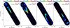 |
Fig. 1 Maps of the CO(2–1) intensity integrated over the EHV and SHV velocity regimes. The velocity ranges of integration are given inside square brackets and are measured with respect to a cloud LSR velocity of 6.7 km s−1. The map coordinates are offsets measured with respect to the position of IRAS 04166, and the color intensity scales at the top are in units of K km s−1. We note the different geometry of the SHV and EHV components. |
3.3 Velocity structure of the IRAS 04166 outflow
The CO(2–1) maps of Fig. 1 provide a first indication of the outflow regular behavior and the strong symmetry between the two lobes. To study in more detail the velocity structure of the outflow, Fig. 3 presents a series of CO(2–1) velocity maps where the two lobes have been oriented vertically so that the gas appears to flow upwards. This has been done by rotating the outflow clockwise by 30.4 degrees, which is the outflow position angle determined by Santiago-García et al. (2009), and by reversing the y-axis in the red lobe. To provide a finer view of the outflow kinematics, the emission range of each lobe has been divided into six velocity intervals of 8 km s−1.
The panels of Fig. 3 provide further evidence of the regular behavior and symmetry of the two outflow components. The three leftmost panels cover the SHV regime and show that the slower outflow gas is distributed in two conical lobes that have almost straight walls and the protostar at their vertex. The maps also show that the emission is significantly brighter toward the edges of the lobes, suggesting that it exhibits limb brightening caused by the gas being preferentially located in shells along the walls.
In addition, the opening angle of the conical lobes decreases slightly with increasing velocity, which is a pattern previously seen in multiple outflows, both having a jet-like EHV component, as in L1448 (Hirano et al. 2006) and HH212 (Lee et al. 2015), and without having a EHV component, as in L1551 (Moriarty-Schieven et al. 1987) and Mon R2 (Meyers-Rice & Lada 1991). This type of pattern suggests that the SHV emission traces a shear flow composed of ambient gas that has been swept-up into shells by a faster outflow component that moves along the center of the lobe. An alternative interpretation in terms of a projection effect caused by gas moving in a hollow cone with constant velocity can be ruled out. This model predicts that after reaching its maximum opening angle, the emission will start to collimate again with decreasing velocity due to the front-back symmetry of the gas moving in a cone. In reality, the emission of each lobe reaches its largest opening angle close to the ambient velocity and then disappears in the following channel maps. This is consistent the physical decrease in velocity expected for a shear flow, and not with a mere projection effect expected for a hollow cone.
An additional feature within the low-velocity maps is the presence of bright lines that emerge near the outflow base and extend almost vertically along the cavity. They are more prominent toward the blue lobe, but they can also be seen in the red lobe with weaker intensity. A possible mechanism for their origin is discussed in Section. 4.5.
The three rightmost panels of Fig. 3 approximately correspond to the EHV regime, and show a very different distribution from that of the SHV gas. At both blue- and redshifted velocities, the EHV emission delineates a series of arcs concave with respect to the protostar that widen gradually with distance. The position of these arcs matches well the position of the EHV peaks previously seen by Santiago-García et al. (2009) and Wang et al. (2014), but the higher sensitivity of the ALMA images reveal now greater amount of detail. In particular, the new ALMA data show that the EHV emission extends over the full width of the SHV lobe, and that it merges smoothly with the side walls. This behavior is best seen in the 26 < |ΔV| < 34 km s−1 velocity range, which represents the transition between the SHV and EHV regimes and therefore contains emission from both velocity components. In these maps, the EHV arcs widen with distance from the protostar and follow the diverging walls of the SHV lobe, suggesting that despite their different geometries, the SHV and EHV outflow components are physically connected. This is a first indication that the EHV gas may play a role in the acceleration of the slower SHV outflow, an issue that is further investigated in Sect. 4 with the help of PV diagrams.
Another notable feature of the EHV emission is its systematic change of shape and position with velocity. At the lowest EHV speeds (26 < |ΔV| < 34 km s−1) the emission is distributed in a series of arcs that are sharply defined and relatively thin. As the velocity increases, the emission of each arc becomes more diffuse and shifts slightly toward the protostar, starting to fill the concave portion of the arc. This behavior is more evident in the most distant EHV peaks of each lobe thanks to their larger separation and limited mutual overlap. One EHV peak in each lobe (the one near Δy = 60″) was studied by Tafalla et al. (2017) using ALMA single-pointing observations, and its velocity pattern was reproduced with a model where the gas is located along a curved disk-like structure that is similar to a bow shock and where the gas is expanding laterally away from the outflow axis. The new ALMA observations show now that this velocity pattern is common to all the EHV peaks, strengthening the interpretation that the EHV peaks represent internal bow shocks caused by a time-variable jet, as proposed by Santiago-García et al. (2009).
To summarize of the main features of the outflow velocity field we present in Fig. 4 maps of the CO(2–1) velocity centroid for the SHV and EHV regimes using the actual orientation of the outflow. The left panel shows that both the blue and red SHV lobes have a layered velocity field with the slower gas (colored red) flowing along the outer boundary of the lobe and the faster gas (yellow to green) flowing interior to it. In contrast, the EHV gas shown in the right panel presents multiple velocity oscillations along the outflow axis. These oscillations arise from the already-mentioned internal velocity structure of the EHV peaks, that have the slowest gas located in the outer part of the arc (red color) and the fastest gas in the inner part (purple). This pattern is more noticeable in the furthermost EHV peaks partly due to their isolation but also partly due to the choice of color scale. The gas in the inner peaks reaches slightly higher velocities, as shown below with PV diagrams, and the color scale has been chosen to emphasize the velocity structure of the outer peaks.
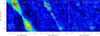 |
Fig. 2 Maps of the combined blueshifted and redshifted EHV emission of CO(2–1), SiO(5–4), and SO(6,5–5,4) toward the inner 25″ × 25″ of the IRAS 04166 outflow. For CO(2–1) and SiO(5–4), the first contour and contour interval are 9 K km s−1, while for the weaker SO(6,5–5,4) they are 3 K km s−1. The map offsets are referred to the position of IRAS 04166. |
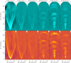 |
Fig. 3 Maps of CO(2–1) intensity integrated over 8 km s−1 intervals to illustrate the different velocity regimes of the IRAS 04166 outflow. For easier comparison, the maps of blueshifted emission (top) have been rotated clockwise by |
![Mathematical equation: $\[30^{\circ}_\cdot4\]$](/articles/aa/full_html/2026/02/aa55924-25/aa55924-25-eq4.png)
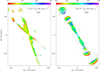 |
Fig. 4 Maps of the absolute value of the velocity centroid of CO(2–1) for the SHV (left) and EHV (right) regimes. IRAS 04166 is located at the origin of coordinates, and the color scales at the top are in units of km s−1. We note the shear pattern in the SHV regime and the velocity oscillations along the outflow axis in the EHV regime. |
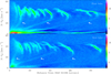 |
Fig. 5 Position–velocity diagrams of the CO(2–1) emission along the axis of the blue (top) and red (bottom) lobes of the IRAS 04166 outflow. The black arrows indicate some of the finger-like features that connect the EHV emission with the origin of the diagram. The velocity scale is measured in absolute value with respect to the cloud LSR velocity (6.7 km s−1), and the wedge scales on the right are in units of K. |
3.4 Connection between the SHV and EHV regimes
As seen in the velocity maps of Fig. 3, the arced EHV emission extends over the full span of the SHV lobes and merges smoothly with their walls, suggesting that the two outflow components, despite their very different velocity signature, are physically connected. To further investigate this possible connection between the EHV and SHV gas, we turn our attention to the PV diagrams of the emission. These diagrams present the outflow velocity in one of their axes, and are therefore better suited to study the continuity of the gas velocity field.
Figure 5 presents PV diagrams of the CO(2–1) emission along the outflow axis for both the blue (top) and red (bottom) lobes. These diagrams have been generated as if a 4″-wide slit had been placed along the outflow axis, although the exact value of the slit width has very little effect on the result. For easier comparison, the two diagrams represent the emission as a function of the absolute velocity displacement with respect to the ambient cloud. Similar diagrams for the SiO(5–4) emission are shown in Fig. A.4, although they are not further discussed due to their low sensitivity and their great similarity with those of CO(2–1).
As can be seen in Fig. 5, the PV diagrams of the blue and red CO(2–1) emission have very similar features. In each diagram, the emission from the EHV gas appears as a series of discrete components centered approximately at |V − V0| ≈ 40 km s−1. Each component presents a similar slanted orientation with a quasi-linear decrease in velocity from about 50 km s−1 to 30 km s−1 as the distance from the protostar increases. This pattern corresponds to the systematic changes in the EHV emission seen in Fig. 3 and the oscillations of Fig. 4. Its repetition over the length of the outflow gives the PV diagram a characteristic sawtooth pattern that was previously identified by Santiago-García et al. (2009) and Wang et al. (2014).
As discussed in Santiago-García et al. (2009), the sawtooth velocity pattern of the EHV gas matches the signature of a chain of internal bow shocks driven by a jet with variable launch velocity. In this type of jet, fast material launched at later times overtakes slower material that had been launched before, and the resulting shock compression ejects gas from the jet sideways. As simulations show, the sawtooth velocity pattern naturally arises in the PV diagram from the combined projection of the forward and lateral velocities of the ejected gas (Stone & Norman 1993; Smith et al. 1997; Rabenanahary et al. 2022; Lora et al. 2024).
An expansion of laterally ejected gas from a jet also can explain the gradual flattening of the sawtooth pattern as a function of distance to the protostar seen in Fig. 5. This behavior is expected from the gradual expansion of the internal bow shocks as they move away from the protostar since the expansion spreads the lateral ejection over a larger spatial scale. This effect is further explored in Sect. 4.4 with the help of a ballistic model, but a similar behavior can be seen in the simulations of Wang et al. (2019), where the flattening is reproduced by the gradual expansion of spherical shells ejected by the protostar.
In addition to the sawtooth pattern, the PV diagram of Fig. 5 shows multiple linear features that connect the EHV peaks with the origin of the diagram. The most prominent ones are indicated with arrows in the figure, and can be seen almost symmetrically in the blue and red lobes. These features are referred to as fingers and have not been previously seen in the IRAS 04166 outflow probably because of their weak emission. A close inspection of the PV diagrams suggests that there may be fingers connected to all EHV peaks, but that only a few are bright enough to be traced back to the origin of the PV diagram. Higher-sensitivity observations are needed to investigate the presence of additional fingers and characterize their global distribution in the outflow.
The presence of fingers in the PV diagram suggests that each EHV peak is followed by a trail of material at intermediate velocities that connects the EHV emission with the protostellar vicinity. If the EHV peaks represent jet gas that has been ejected laterally due to internal shocks, the fingers would appear to correspond to the fraction of ejected gas that has been left behind due to its interaction with the surrounding medium. Each EHV peak, therefore, likely represents the forward part of a shell of ejected gas, and since the fingers can be traced back to the protostellar vicinity, the responsible lateral ejection has to have begun close to the protostar.
This interpretation of the fingers is supported by the simulations of the interaction between a pulsating jet and its surrounding dense core presented by Rabenanahary et al. (2022). As can be seen in their Fig. 9(c), the PV diagram of material that has been accelerated by a pulsating jet presents a set of finger-like extensions that connect the origin of the diagram with the peaks in the jet. The presence of these fingers indicates that linear momentum is being transferred from the EHV gas to the SHV regime, slowing down the former and accelerating the latter.
If the fingers represent shells of gas expanding in the wake of an EHV ejection, they are expected to appear as a series of ring-like structures in PV diagrams perpendicular to the outflow, as shown by Rabenanahary et al. (2022) in their Fig. 10. Our PV diagrams of the IRAS 04166 outflow are significantly limited in sensitivity due to the short integration time of the observations, but as shown in Fig. A.5, they do suggest the presence of ring-like cavities at intermediate velocities. We therefore conclude that the main features in the outflow PV diagrams, both parallel and perpendicular to the jet direction, are best interpreted as resulting from the lateral ejection of jet material and the interaction of this material with the environment. To further test this interpretation, we present in Sect. 4.2 the results of a ballistic model of the interaction between gas ejected laterally from a jet and the surrounding outflow material. While highly simplified, our model allows exploring the velocity field of the ejections needed to fit the PV diagram along the IRAS 04166 outflow, and should be seen as a first step toward a more comprehensible analysis to be carried out using numerical simulations.
4 Discussion
4.1 Comparison to other outflows
The IRAS 04166 outflow is unusual for having an EHV component of high symmetry and collimation, but many of its other emission features have counterparts in less-extreme systems. The presence of multiple outflow shells, for example, has been previously reported in different outflows, especially when observed with ALMA. Lee et al. (2015) found a very clean case of this type of geometry in the HH 212 outflow, where multiple nested shells can be seen in the CO emission connecting the vicinity of the central source to the jet bow shocks seen in H2. Prominent nested shells can also be seen in the CO emission of the highly collimated CARMA-7 outflow mapped by Plunkett et al. (2015), and similar structures have been reported more recently by de Valon et al. (2022), Omura et al. (2024), and Liu et al. (2025). This frequent finding of discrete shell structures super-imposed on the large-scale emission from the bipolar outflow strongly suggest that episodic ejection events play a prominent role in the mechanism of gas acceleration.
Another feature with counterparts in several outflows is the sawtooth velocity pattern of the EHV gas. Hirano et al. (2010) found evidence for a similar pattern in the EHV gas of the L1448 outflow, and Gavino et al. (2024) have recently presented a clean case of this type of pattern in the jet-like outflow powered by BHR 71-IRS2. Other outflows with evidence for a sawtooth velocity pattern include those powered by MMS5/OMC-3 (Matsushita et al. 2019), HH270mm1-A (Omura et al. 2024), and several sources mapped by the ALMASOP project (Dutta et al. 2024; Liu et al. 2025). In the case of HOPS 315, the pattern is accompanied by finger-like extensions toward the origin of the PV diagram like those seen in IRAS 04166, and Liu et al. (2025) interpret them as resulting from the bubble structure of the unified outflow model of Shang et al. (2023). Additional evidence for finger-like extensions in an outflow PV diagram has been presented by Plunkett et al. (2015) for the case of CARMA-7, although the low velocity of that outflow due to its high inclination angle makes it difficult to discern whether the fingers are connected to a sawtooth velocity pattern in the jet component.
Even outflows without evidence for an EHV component have been found to present finger-like features like those seen in IRAS 04166. Arce et al. (2013) and Zhang et al. (2019) have reported the presence of multiple finger-like shells in the PV diagrams along the HH 46/47 outflow. Additional evidence for PV fingers has been presented by Nony et al. (2020) in several outflows of the W43-MM1 protocluster, Vazzano et al. (2021) in the outflows of the low-mass Lupus cloud, and de Valon et al. (2022) in the outflow of DG Tauri B. In all these cases, the fingers have been interpreted as resulting from some type of episodic event in the outflow driving agent, although the nature of this agent has been variously assumed to be a wide-angle component (Arce et al. 2013; Zhang et al. 2019; Vazzano et al. 2021), a collimated jet (Nony et al. 2020), or an MHD disk wind (de Valon et al. 2022).
The finding of shells, sawtooth patterns, and PV fingers in outflows that are at different evolutionary stages and located in different environments suggests that these features may represent a frequent component of the outflow phenomenon that needs to be better understood. In this respect, the IRAS 04166 outflow, with its simple geometry and high degree of symmetry, offers an ideal target to model the origin of these different features and to test whether they could result from the interaction of a time-variable jet with its surrounding medium. Given the limited number of simulations of realistic jets available, we rely for our analysis on a highly idealized model of the interaction between gas ejected from a pulsating jet and its surrounding medium that is presented in the next section.
4.2 A toy model of the lateral ejection from a jet
As we have seen, the simulations of pulsating jets by Stone & Norman (1993) and Rabenanahary et al. (2022) predict features in the emission maps and PV diagrams that resemble those found in the IRAS 04166 outflow. Unfortunately, these simulations cannot be easily compared to our ALMA data since they assume specific jet and cloud conditions that do not necessarily coincide with those of the IRAS 04166 outflow. To further investigate the origin of the features seen in the IRAS 04166 outflow, we present a highly simplified model of the interaction between gas ejected sideways by an internal shock in a jet and the surrounding outflow material. Given its simplicity, we consider this model only as a first step toward a more realistic description of the interaction between a jet shock and its surrounding flow.
Fig. 6 presents a schematic view of how the model simulates the evolution of a single lateral ejection produced by an internal shock in a jet. The model assumes that the jet propagates along the y-axis, and that due to some type of velocity variability, it develops an internal working surface (IWS) of high compression (Raga et al. 1990). This IWS moves along the y-axis and ejects gas perpendicular to its motion. The ejected gas interacts with the surrounding outflow material, and due to the ensuing compression and possible heating, the combined ejected plus swept up material produces a visible signal in the outflow emission. The goal of the model is to follow the path of the ejected gas as it moves through the surrounding medium, and to calculate how much mass is swept up in the process assuming conservation of linear momentum. To keep the calculation as simple as possible, the ejected gas is treated as a set of independent particles that move away from the jet beam with a given perpendicular velocity in addition to their initial jet velocity.
A critical ingredient of the model is the velocity field assumed for the gas that surrounds the jet. This gas has been accelerated by multiple previous ejections, and therefore has a potentially complex kinematics that can only be treated in a highly idealized way. As mentioned in Sect. 3.3, the velocity of the SHV component in the IRAS 04166 outflow decreases gradually toward the walls of the lobes and follows a shear-flow pattern. Similar shear-flow patterns are predicted by the simulations of jet-driven outflows by Rabenanahary et al. (2022) as a result of the interaction between multiple shocks from successive jet ejections (their Sect. 5.2), and by the model of a wide-angle wind of Shang et al. (2006, 2020, 2023) as an intrinsic property of the outflow (see also Liang et al. 2020). Following these theoretical results, we model the gas around the jet as having a shear-flow pattern in which the material flows radially from the protostar with a speed that depends on the angle θ with respect to the jet direction (Fig. 6). For continuity, the flow velocity is assumed to match the jet velocity along the y-axis (θ = 0) and to decrease gradually until reaching a zero value at θmax, which represents the boundary between the outflow and the ambient cloud. Since the model is highly idealized and its goal is to reproduce the general behavior of the EHV emission, we choose the following simple velocity field that satisfies the above constraints:
![Mathematical equation: $\[v_{\mathrm{r}}(\theta)=v_{\mathrm{jet}} ~\cos ^2\left(\frac{\pi}{2} \frac{\theta}{\theta_{\mathrm{max}}}\right).\]$](/articles/aa/full_html/2026/02/aa55924-25/aa55924-25-eq5.png) (1)
(1)
Here vr is the radial velocity of the gas, vjet is the jet forward velocity, and θmax is the outflow half opening angle (Fig. 6).
To complete the description of the gas surrounding the jet we need to model its density profile. The maps of Fig. 1 show the SHV component as a limb-brightened conical shell, indicating that its density must increase toward the outer walls of the outflow. A similar gas distribution is predicted by the simulations of Rabenanahary et al. (2022) (their Sect. 5.2), so favoring again a simple expression, we choose a density profile of the form
![Mathematical equation: $\[n_{\text {shell }}(r, \theta)=n_0(r) ~\cos ^{-2}\left(\frac{\pi}{2} \frac{\theta}{\theta_{\max }}\right),\]$](/articles/aa/full_html/2026/02/aa55924-25/aa55924-25-eq6.png) (2)
(2)
where n0(r) is a fiducial density that in principle could depend on the distance to the protostar r. This dependence is likely flatter than the r−2 expected for conservation of mass since the outflow consists of ambient accelerated gas that is gradually being entrained along the cavity walls (plus an additional contribution from ejected jet material). To test the sensitivity of our results to the assumed radial dependence of the density profile, we run models of the best-fit solution (described in the next section) using n0(r) factors with r−2, r−1, and no radial dependence. The resulting PV diagrams (shown in Fig. A.6) indicate that the radial dependence of the density profile plays a minimal role in the solution so, for simplicity, we take n0(r) as a constant value.
Having defined the environment where the ejection propagates, the model follows a set of particles of given initial mass and density that are ejected from the IWS as it moves at constant velocity along the jet axis. The trajectory of each particle is determined at consecutive time steps by requiring conservation of the combined linear momentum of the ejected gas and the swept-up material. At a chosen time, the positions and velocities of the particles can be used to generate the PV diagram that results from an observation from an arbitrary angle with respect to the jet axis. Given the assumptions of the model, we refer to it as the LEAF (Lateral Ejection onto an Angle-dependent Flow) model. We note that given its simplicity, the model cannot be used to investigate the nature of the jet-like wind (pure jet, disk wind, or X-wind) but only its effect on the surrounding medium.
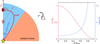 |
Fig. 6 Left: geometry assumed for the simple model of lateral ejection from an internal working surface (IWS) presented in Sect. 4.2 (only one outflow quadrant is shown). The IWS moves along the y-axis with a constant vjet velocity and ejects gas with a vside perpendicular component. The ejected gas interacts with a surrounding shear flow and forms a shell that surrounds the jet axis (red solid curve). The plot shows the current location of the IWS (solid) and its position approximately half way along its path (dotted). The red dotted line represents the approximate trajectory between time of ejection and current time. The model predicts the expected PV diagram from an observation made at an arbitrary angle from the jet axis. Right: velocity and density profiles as a function of angle from the jet axis used to simulate the outflow shear flow. They correspond to Eqs. (1) and (2) in the text. |
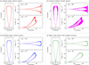 |
Fig. 7 Summary of results from modeling four different modes of lateral ejection from a jet. Each mode is represented by a quadrant, and is labeled with its kinematic characteristics and color-coded for easier reference. In each quadrant, the vertical diagram represents a map of the ejected gas, and two horizontal diagrams are position–velocity plots for inclinations of 90° for a jet moving in the plane of sky and 47° for expected inclination of the IRAS 04166 outflow (see text for details). |
4.3 Different modes of lateral ejection and their signature in the PV diagram
As a first application of the LEAF model, we investigated how the properties of a lateral ejection affect the PV diagram. For this, we run different cases varying the two main parameters that seem to control the evolution of the ejected gas in the model: the rate at which the IWS ejects material laterally and the distribution of velocities in the ejected gas. To explore the effect of the ejection rate, we compared cases where the IWS ejects material continuously as it propagates along the jet axis with cases where the material is ejected in a single event. To investigate the effect of the distribution of ejection velocities, we compared cases where all the ejected gas has the same lateral velocity with cases where the ejected gas contains a mix of lateral velocities. To simplify the discussion, here we present the results from four types of ejection that reproduce some of the features seen in the PV diagrams of the IRAS 04166 outflow: (a) continuous ejection with a single lateral velocity, (b) continuous ejection with multiple lateral velocities, (c) continuous ejection with a single decreasing velocity, and (d) single-event ejection with multiple lateral velocities.
Figure 7 summarizes the main results of our model exploration by presenting the output of each case in one quadrant. The elongated diagram on the left of each quadrant represents the unprojected map of the ejected material, and the two plots to its right represent PV diagrams along the outflow axis. The top one corresponds to an inclination of 90° (jet moving in the plane of the sky) and the bottom one to an inclination of 47°, which is the value estimated for IRAS 04166 by the eDisk project from a fit to the disk emission (Ohashi et al. 2023; Phuong et al. 2025). We prefer this value to the similar one of 52° derived by Tafalla et al. (2017) because the disk measurement is likely more accurate than an estimate based on the outflow emission, although the exact choice of angle has little influence in our analysis.
Since the LEAF model solves the ejection of gas in a single plane, we simulated the three-dimensional structure of the outflow by combining multiple LEAF solutions, each representing the ejection of gas in a different plane around the jet axis. Using this set of LEAF solutions, we generated the PV diagram expected from an observation along the jet axis with a slit 4 arcsec wide like that used with the IRAS 04166 outflow in Fig. 5. In all models, we assumed a jet velocity of 61 km s−1 for consistency with Tafalla et al. (2017), and we followed the ejection of jet material for 650 yr, which is the time needed to match the position of one of the IRAS 04166 EHV peaks in the PV diagram (Sect. 4.4).
As can be seen in Fig. 7, the panels that represent the maps of the ejected material for all four ejection cases show similar distributions that broadly resemble the individual outflow shells of IRAS 04166 seen in Fig. 3. While this good match reinforces the lateral-ejection interpretation of the shell geometry, it also shows that the spatial distribution of the ejected gas can be fit using different ejection options, so it does not provide a strong constraint on the gas kinematics.
In contrast with the maps, the PV diagrams of Fig. 7 show a variety of shapes that suggests they are more sensitive to differences in the mode of ejection. Our first model (top left quadrant) assumed that the IWS moves along the jet axis and simultaneously ejects material laterally at a constant rate and with a single velocity of 15 km s−1. This velocity choice is in line with the estimate from Ostriker et al. (2001), who predicted that in the bow shock of a protostellar jet the gas is heated to 104 K and ejected with a speed of ~ ![Mathematical equation: $\[\sqrt{5}\]$](/articles/aa/full_html/2026/02/aa55924-25/aa55924-25-eq7.png) times the sound speed. If the jet is moving in the plane of the sky (90° inclination), the predicted PV diagram presents a trumpet shape with two branches that diverge with distance from the central source and are connected by a straight line at the IWS position. This connection arises from jet gas that moves away from the jet axis at different angles with respect to the line of sight and therefore is projected inside the slit at intermediate velocities. The trumpet shape resembles that predicted by more realistic models of a single bow shock, like those of Ostriker et al. (2001) (their Fig. 3) and Lee et al. (2001) (their Fig. 5). These models also assumed a constant lateral ejection velocity, so their agreement with our predicted PV diagram suggests that despite its simplicity, the LEAF model captures the basic kinematic properties of the of lateral ejection. For an inclination angle of 47°, the LEAF model predicts a connection between the two branches of the PV diagram that has a complex bow-tie shape structure and differs significantly from the smooth linear distribution seen in the IRAS 04166 PV diagram (Fig. 5). We therefore conclude that a lateral ejection model having a constant single velocity fails to reproduce the observed PV diagram.
times the sound speed. If the jet is moving in the plane of the sky (90° inclination), the predicted PV diagram presents a trumpet shape with two branches that diverge with distance from the central source and are connected by a straight line at the IWS position. This connection arises from jet gas that moves away from the jet axis at different angles with respect to the line of sight and therefore is projected inside the slit at intermediate velocities. The trumpet shape resembles that predicted by more realistic models of a single bow shock, like those of Ostriker et al. (2001) (their Fig. 3) and Lee et al. (2001) (their Fig. 5). These models also assumed a constant lateral ejection velocity, so their agreement with our predicted PV diagram suggests that despite its simplicity, the LEAF model captures the basic kinematic properties of the of lateral ejection. For an inclination angle of 47°, the LEAF model predicts a connection between the two branches of the PV diagram that has a complex bow-tie shape structure and differs significantly from the smooth linear distribution seen in the IRAS 04166 PV diagram (Fig. 5). We therefore conclude that a lateral ejection model having a constant single velocity fails to reproduce the observed PV diagram.
As an alternative model, we explored a case where the IWS moves along the jet axis and simultaneously ejects material with a mixture of lateral velocities. For simplicity, we assumed that the mixture is uniformly distributed between zero and 15 km s−1 (the velocity of the single-velocity model), and present the results in the top right quadrant of Fig. 7. As can be seen, the PV diagram for an inclination of 90° consists of a cloud of points whose outer envelope coincides with the single-velocity model, but is now filled with points toward the end of the diagram. For an inclination of 47°, the PV diagram resembles that of the single-velocity model, but has a broader distribution of points at high velocities that contrasts with the thin EHV features seen in the IRAS 04166 PV diagram. A multiple-velocity model, therefore, also fails to reproduce the observations.
The failure of models with a constant rate of ejection reinforces the analysis of Tafalla et al. (2017), who found that to model the emission from two EHV condensations, the lateral velocity of the gas had to increase linearly with distance from the jet axis. To achieve this, two possible mechanisms were suggested: (i) the velocity of the lateral ejection decreases linearly with time, or (ii) the ejection occurs during a single event that generates multiple lateral velocities, and the material orders itself into a Hubble flow as it expands sideways. Our next two models explored these two options.
To model an ejection with a decreasing lateral velocity we assumed that the IWS starts ejecting gas laterally at 15 km s−1 when close to the protostar, and that the lateral velocity decreases linearly as the IWS advances, until it reaches zero at the time the system is observed. As can be seen in the bottom left quadrant of Fig. 7, the resulting PV diagrams present a smooth distribution that for an inclination of 47° matches reasonably well the shape of the individual features of the IRAS 04166 PV diagram. In this respect, a model with decreasing ejection velocity seems to provide a reasonable fit to the ALMA observations. A caveat, however, is that the model requires that by the time when the system is observed, the ejection velocity has decreased from its initial high value to zero, or otherwise the PV diagram would include a bow-tie structure similar to that seen in our first model. Since none of the EHV peaks in the PV diagram of the IRAS 04166 outflow presents this type of structure, the condition of having reached zero velocity has to be satisfied by all the outflow ejections, no matter how close they are located from the protostar (and therefore how young they are). This suggests that the ejection velocity has to decrease very rapidly from its initial value to zero.
A lateral ejection whose velocity decreases rapidly to zero is practically equivalent to an ejection that releases the gas instantaneously with a distribution of velocities between a maximum value and zero. This type of ejection was the second alternative proposed in Tafalla et al. (2017) to fit their observations, and is the final ejection case that we explored using the LEAF model. To follow its evolution, we assumed that the ejection takes place when the IWS is at a very small distance from the protostar, which we took as the size of the first time step to avoid possible divergences caused by the zero radius at the origin. This instantaneous ejection was assumed to release gas that has a uniform mix of lateral velocities between zero and 15 km s−1. As shown in the bottom right quadrant of Fig. 7, the predicted PV diagram for an inclination of 47° reproduces well the main characteristics of each EHV peak in the IRAS 04166 outflow: a fast regime where the velocity decreases linearly with distance from the protostar and finger-like extensions that connect the fastest emission to the origin of the PV diagram. A single-event ejection containing multiple lateral velocities therefore provides the best fit to the PV diagram of the individual EHV peaks in the IRAS 04166 outflow.
While the results of our simple LEAF model need confirmation using more realistic simulations, they already provide some clues on how the different features of the PV diagram may arise from the lateral ejection of jet material. For the case of a single-event ejection, the LEAF model suggests that the ejected gas leaves the IWS moving with a combination of a forward jet velocity and a lateral component that lies in the range from zero to about 15 km s−1. The gas ejected with the largest lateral velocities moves rapidly away from the jet axis and sweeps gas of increasing density from the surrounding shear flow, slowing down in the process. This fraction of gas gives rise to the PV fingers, which are therefore composed of a mix of original ejected material and swept-up surrounding gas. In contrast with this rapidly decelerated gas, the fraction of material ejected with a small lateral velocity component moves along the jet direction and suffers less deceleration from its interaction with the surrounding shear flow due to the combined effect of the high velocity of the shear flow close to the jet axis and its lower volume density. As this gas moves forward, it also spreads laterally and acquires a Hubble-law distribution with respect to the jet axis, giving the head of the PV diagram its characteristic slanted shape This fraction of gas corresponds to the EHV component, and is distributed spatially as a flattened, curved bow shock. In this respect, the description of the EHV component inferred from the LEAF model is consistent with the more-ad hoc parameterization used in Tafalla et al. (2017) to reproduce the velocity maps of the EHV emission using a parabolic distribution of expanding gas. The advantage of the new LEAF model is that in addition to fitting the kinematics of the EHV gas it automatically reproduces the finger features that connect the EHV emission with the origin of the PV diagram.
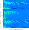 |
Fig. 8 Comparison between the PV diagram from a multi-ejection model (middle) and the ALMA observations of the IRAS 04166 outflow (as shown in Fig. 5). The intensity scale of the model is linear but arbitrary since it is simply scaled from the amount of ejected plus swept-up gas. |
4.4 Simulating the multiple ejection events of the IRAS 04166 PV diagram
Having reproduced the shape of the individual PV-diagram features assuming an instantaneous ejection, we attempted to model the full EHV emission of the IRAS 04166 outflow by simulating a sequence of successive ejections that travel along the jet axis. For this we run multiple instances of the LEAF model using the same physical conditions for the jet and the shear flow, and only varied the time at which each ejection was emitted.
From the PV diagram of the blue lobe, which shows a brighter and cleaner pattern, we estimated that there are at least eight separate ejections propagating in the region mapped with ALMA. This number is higher by one than estimated by Santiago-García et al. (2009) from their lower-sensitivity data, although the exact value is still uncertain due to the complexity of the emission near the protostar, where some of the ejections lie very close to each other and may be interacting among themselves. This uncertainty is not critical for our model since we did not aim to fit exactly the emission but to show how its main features can be understood as a resulting from the propagation of multiple ejection events.
To determine the age of each EHV peak, we followed with the LEAF model the evolution of the ejected gas from its launching point near the protostar to its current position. As before, we assumed a constant jet velocity of 61 km−1 and an inclination with the line of sight of 47°. Since the jet velocity and the shear-flow conditions are assumed to be the same for all the ejections, the sequence of the eight model ejections can also be seen as a time series in the propagation of a single generic ejection. By fitting the position of their EHV heads, we found that the eight episodes need to have the following approximate ages: 120, 180, 310, 400, 500, 650, 850, and 1350 yr.
While the above values do not indicate a strictly periodic pattern, we note that the first six episodes have relative separations close to 100 yr, after which the time between episodes increases significantly. Similar patterns of increasing separation between ejection events are seen in some HH jets (Reipurth & Bally 2001), and may arise from the gradual fading of some ejections as they move away from the protostar or from the dissociation of CO in particularly strong shocks. If this is the case in IRAS 04166, our results suggest that the outflow lateral ejections have a typical time scale of around 100 yr. This time scale most likely reflects some type of variability in the accretion process since the central source appears to be single (Phuong et al. 2025).
Although the LEAF model simulates the kinematics of the ejected gas and predicts its location on the PV diagram, it does not solve the equation of radiative transfer, so it cannot be used to derive line intensities. We can still estimate an approximate level of EHV emission by using the distribution of moving mass and assuming that the CO(2–1) emission is optically thin. This assumption is consistent with our lack of detection of 13CO(2–1) in the EHV regime and with the quantitative analysis of the emission by Tafalla et al. (2010). Using this approximation, and convolving the resulting PV diagram with a small kernel to simulate a finite duration of the ejection event and the jet velocity dispersion, we obtained the PV diagram shown in the middle panel of Fig. 8.
As can be seen in Fig. 8, a model with multiple instantaneous ejections reproduces most of the features seen in the PV diagram, including the sawtooth appearance of the EHV emission and the presence of low-velocity fingers connecting the EHV emission with the origin of the diagram. It also reproduces the gradual flattening of the sawtooth pattern as the ejections move away from the protostar. This behavior results from the lateral expansion of the ejected gas, which stretches its emission along the spatial axis of the PV diagram while it maintains a constant velocity spread (see Wang et al. 2019 for a similar interpretation in terms of expanding spherical shells). Another feature seen both in the data and the model is the relatively weak emission of the low-velocity fingers. Unfortunately the ALMA observations are not sensitive enough to reveal the full complexity of the overlapping emission from the fingers that is expected in the model, so it is not possible to use these features to further constrain the interaction between the EHV and SHV gas.
While not directly predicted by our model, the interpretation of the EHV gas as a lateral jet ejection that propagates into the surrounding medium can also help explain the bright trails seen to radiate from the inner outflow and extend almost vertically in the low-velocity maps of Fig. 3. These trails could represent lateral ejections that due to an anisotropy in their launching are impacting the surrounding gas in a preferential direction as they propagate along the outflow. Further observations of these features are needed to better constrain their velocity pattern.
4.5 Evolution and detectability of the unperturbed jet
The interpretation of the EHV emission as representing jet material that has been ejected laterally by internal shocks raises the question of whether there is any evidence in the data for jet gas that has not yet undergone a shock interaction. Graphic depictions and models of jet-driven outflows often show a jet component traveling between consecutive internal working surfaces that has not yet encountered an internal shock (e.g., Fig. 1 in Raga et al. 1993 or Fig. 19 in de Valon et al. 2022). The IRAS 04166 data, however, do not show any evidence for such an unperturbed jet component, and the only emission features that could potentially be associated with a pristine jet are the two unresolved EHV peaks seen toward the protostar vicinity in SiO(5–4) (see Fig. 2). All EHV emission at further distances from the protostar displays the characteristic sawtooth velocity pattern that we have associated with laterally expanding jet gas.
While it is still possible that an unperturbed jet component remains undetected because it has an atomic composition, this seems unlikely since it would require that the jet gas becomes molecular almost instantaneously after being ejected by the shock. It seems more likely that the lack of detection of unperturbed jet material between the EHV peaks arises because most (or all) the original protostellar jet has been converted into laterally expanding gas. This interpretation agrees with the LEAF model analysis, which requires that the ejection of gas from the jet occurs almost instantaneously in the vicinity of the protostar. It also helps to understand the lack of significant emission of optical and IR shock tracers along the jet axis, which was mentioned in the introduction. Any shocks responsible for the lateral ejection of jet gas must have occurred in the protostellar vicinity, which is highly extincted.
Whether the above interpretation agrees with published simulations of time-varying jets is less clear, although we note that Stone & Norman (1993) state that the jet beam in their simulations is rapidly depleted (“starved”) due to the lateral ejection of material by the internal shocks. A detailed study of the survival of unperturbed jet material using numerical simulations would be highly desirable to clarify our understanding of jet propagation and evolution.
To summarize, the picture that emerges from the IRAS 04166 data is one where a protostellar jet is ultimately responsible for the production of the EHV component via internal shocks. These shocks, in turn, lead to a rapid destruction of the jet and its conversion into a series of forward-moving, but also laterally expanding shells of gas. Whether a similar scenario is applicable to other outflows still needs further investigation, but the presence of finger-like structures in other systems suggests that this is a realistic possibility. Since many of these outflows lack an EHV component in molecular lines, we have to assume that the gas ejected from the jet in those cases has an atomic composition, and that the finger signatures in these outflows represent ambient material that has been accelerated by the atomic component. A more systematic investigation of the frequency and properties of finger structures in other outflows is necessary to test this scenario.
5 Conclusions
We observed the IRAS 04166 outflow with the 12m and Compact Arrays of ALMA using the Band 6 receivers and focusing on the CO(2–1) emission. We also developed a simplified model of the evolution of gas ejected laterally from a jet by an internal working surface, and we used this model to interpret the PV diagrams of the CO(2–1) emission. From this work, we have reached the following main conclusions:
1. In agreement with previous observations, we find that the IRAS 04166 outflow comprises two regimes that we refer to as the SHV and EHV components. The SHV component appears in the maps as a pair of limb-brightened conical shells where the gas follows a shear-flow velocity pattern. The EHV component lies internal to the SHV shells and appears in the maps as a series of arcs similar to bow shocks. Each of these arcs presents a similar velocity pattern with the faster gas located closer to the protostar and the slower gas at larger distances;
2. The new ALMA data reveal a previously unseen connection between the SHV and EHV components of the outflow. The velocity maps show that the EHV arcs span the full width of the SHV shells and merge smoothly with their walls. PV diagrams of the emission along the outflow axis show finger-like features that connect the EHV emission with the origin of the diagram. These features suggests that as it moves forward, the EHV-emitting gas leaves behind a trail of gas that has decelerated due to its interaction with the surrounding SHV component;
3. A simple model of the lateral ejection of gas from an internal working surface can reproduce both the velocity pattern of the EHV gas and the presence of the finger extensions. For this to happen, the gas needs to have been ejected almost instantaneously close to the protostar. According to this model, the EHV gas and the finger extensions represent different parts of the ejected gas that started their expansion with different amounts of lateral velocity. Using this model, it is possible to reproduce the PV diagram of the outflow assuming that there have been eight ejections with a typical separation of a hundred years;
4. If the EHV emission represents material that has been ejected from a jet near the protostar, no emission in the data seems associated with a component of the jet that has not yet undergone shock interaction (with the possible exception of unresolved emission toward the protostar). The data therefore suggests that the jet is fully disrupted by the internal shocks early on in its propagation, and that any later interaction between the jet material and the surrounding gas occurs through the expansion of the laterally ejected gas. In the IRAS 04166 outflow this interaction is manifested through the finger structures in the PV diagram. Similar fingers in other outflows may also result from lateral ejections from a jet, although in many cases the ejected gas must be atomic given the lack of molecular EHV emission. Further analysis of finger structures in other outflows is needed to test this scenario.
Acknowledgements
We thank John Bally for his insightful referee’s reports that helped us refine this work. M.T. acknowledges partial support from project PID2019-108765GB-I00 funded by MCIN/AEI/10.13039/501100011033. D.J. is supported by NRC Canada and by an NSERC Discovery Grant. H.S. acknowledges grant support from the National Science and Technology Council (NSTC) 113-2112-M-001-008 and 114-2112-M-001-001-. This paper makes use of the following ALMA data: ADS/JAO.ALMA#2021.1.00575.S. ALMA is a partnership of ESO (representing its member states), NSF (USA) and NINS (Japan), together with NRC (Canada), MOST and ASIAA (Taiwan), and KASI (Republic of Korea), in cooperation with the Republic of Chile. The Joint ALMA Observatory is operated by ESO, AUI/ NRAO and NAOJ. This research has made use of NASA’s Astrophysics Data System Bibliographic Services and the SIMBAD database, operated at CDS, Strasbourg, France.
References
- Arce, H. G., Mardones, D., Corder, S. A., et al. 2013, ApJ, 774, 39 [CrossRef] [Google Scholar]
- Bachiller, R. 1996, ARA&A, 34, 111 [Google Scholar]
- Bachiller, R., Cernicharo, J., Martin-Pintado, J., Tafalla, M., & Lazareff, B. 1990, A&A, 231, 174 [NASA ADS] [Google Scholar]
- Bally, J. 2016, ARA&A, 54, 491 [Google Scholar]
- Bohlin, R. C., Savage, B. D., & Drake, J. F. 1978, ApJ, 224, 132 [Google Scholar]
- Bontemps, S., Andre, P., Terebey, S., & Cabrit, S. 1996, A&A, 311, 858 [NASA ADS] [Google Scholar]
- Bracco, A., Palmeirim, P., André, P., et al. 2017, A&A, 604, A52 [NASA ADS] [CrossRef] [EDP Sciences] [Google Scholar]
- CASA Team (Bean, B., et al.) 2022, PASP, 134, 114501 [NASA ADS] [CrossRef] [Google Scholar]
- Codella, C., Cabrit, S., Gueth, F., et al. 2007, A&A, 462, L53 [NASA ADS] [CrossRef] [EDP Sciences] [Google Scholar]
- Cornwell, T. J. 2008, IEEE J. Sel. Top. Signal Process., 2, 793 [Google Scholar]
- Davis, C. J., Chrysostomou, A., Hatchell, J., et al. 2010, MNRAS, 405, 759 [NASA ADS] [Google Scholar]
- de Valon, A., Dougados, C., Cabrit, S., et al. 2022, A&A, 668, A78 [NASA ADS] [CrossRef] [EDP Sciences] [Google Scholar]
- Dutta, S., Lee, C.-F., Johnstone, D., et al. 2024, AJ, 167, 72 [Google Scholar]
- Ediss, G. A., Carter, M., Cheng, J., et al. 2004, in Fifteenth International Symposium on Space Terahertz Technology, ed. G. Narayanan, 181 [Google Scholar]
- Eswaraiah, C., Li, D., Furuya, R. S., et al. 2021, ApJ, 912, L27 [NASA ADS] [CrossRef] [Google Scholar]
- Frank, A., Ray, T. P., Cabrit, S., et al. 2014, in Protostars and Planets VI, eds. H. Beuther, R. S. Klessen, C. P. Dullemond, & T. Henning, 451 [Google Scholar]
- Gavino, S., Jørgensen, J. K., Sharma, R., et al. 2024, ApJ, 974, 21 [NASA ADS] [CrossRef] [Google Scholar]
- Glassgold, A. E., Mamon, G. A., & Huggins, P. J. 1991, ApJ, 373, 254 [NASA ADS] [CrossRef] [Google Scholar]
- Guilloteau, S., Bachiller, R., Fuente, A., & Lucas, R. 1992, A&A, 265, L49 [NASA ADS] [Google Scholar]
- Hacar, A., Tafalla, M., Kauffmann, J., & Kovács, A. 2013, A&A, 554, A55 [NASA ADS] [CrossRef] [EDP Sciences] [Google Scholar]
- Hirano, N., Liu, S.-Y., Shang, H., et al. 2006, ApJ, 636, L141 [NASA ADS] [CrossRef] [Google Scholar]
- Hirano, N., Ho, P. P. T., Liu, S.-Y., et al. 2010, ApJ, 717, 58 [NASA ADS] [CrossRef] [Google Scholar]
- Högbom, J. A. 1974, A&AS, 15, 417 [Google Scholar]
- Kepley, A. A., Tsutsumi, T., Brogan, C. L., et al. 2020, PASP, 132, 024505 [Google Scholar]
- Kerr, A. R., Pan, S. K., Lauria, E. F., et al. 2004, in Fifteenth International Symposium on Space Terahertz Technology, ed. G. Narayanan, 55 [Google Scholar]
- Kristensen, L. E., van Dishoeck, E. F., Tafalla, M., et al. 2011, A&A, 531, L1 [NASA ADS] [CrossRef] [EDP Sciences] [Google Scholar]
- Krolikowski, D. M., Kraus, A. L., & Rizzuto, A. C. 2021, AJ, 162, 110 [NASA ADS] [CrossRef] [Google Scholar]
- Lee, C.-F. 2020, A&A Rev., 28, 1 [Google Scholar]
- Lee, C.-F., Stone, J. M., Ostriker, E. C., & Mundy, L. G. 2001, ApJ, 557, 429 [NASA ADS] [CrossRef] [Google Scholar]
- Lee, C.-F., Ho, P. T. P., Palau, A., et al. 2007, ApJ, 670, 1188 [NASA ADS] [CrossRef] [Google Scholar]
- Lee, C.-F., Hirano, N., Zhang, Q., et al. 2015, ApJ, 805, 186 [NASA ADS] [CrossRef] [Google Scholar]
- Liang, L., Johnstone, D., Cabrit, S., & Kristensen, L. E. 2020, ApJ, 900, 15 [NASA ADS] [CrossRef] [Google Scholar]
- Liu, C.-F., Shang, H., Johnstone, D., et al. 2025, ApJ, 979, 17 [Google Scholar]
- Lora, V., Nony, T., Esquivel, A., & Galván-Madrid, R. 2024, ApJ, 962, 66 [Google Scholar]
- Masson, C. R., & Chernin, L. M. 1993, ApJ, 414, 230 [Google Scholar]
- Matsushita, Y., Takahashi, S., Machida, M. N., & Tomisaka, K. 2019, ApJ, 871, 221 [Google Scholar]
- Meyers-Rice, B. A., & Lada, C. J. 1991, ApJ, 368, 445 [Google Scholar]
- Moriarty-Schieven, G. H., Snell, R. L., Strom, S. E., et al. 1987, ApJ, 319, 742 [Google Scholar]
- Motte, F., & André, P. 2001, A&A, 365, 440 [NASA ADS] [CrossRef] [EDP Sciences] [Google Scholar]
- Nony, T., Motte, F., Louvet, F., et al. 2020, A&A, 636, A38 [NASA ADS] [CrossRef] [EDP Sciences] [Google Scholar]
- Ohashi, N., Tobin, J. J., Jørgensen, J. K., et al. 2023, ApJ, 951, 8 [NASA ADS] [CrossRef] [Google Scholar]
- Omura, M., Tokuda, K., & Machida, M. N. 2024, ApJ, 963, 72 [Google Scholar]
- Ossenkopf, V., & Henning, T. 1994, A&A, 291, 943 [NASA ADS] [Google Scholar]
- Ostriker, E. C., Lee, C.-F., Stone, J. M., & Mundy, L. G. 2001, ApJ, 557, 443 [NASA ADS] [CrossRef] [Google Scholar]
- Phuong, N. T., Lee, C. W., Tobin, J. J., et al. 2025, ApJ, 992, 18 [Google Scholar]
- Plunkett, A. L., Arce, H. G., Mardones, D., et al. 2015, Nature, 527, 70 [NASA ADS] [CrossRef] [Google Scholar]
- Rabenanahary, M., Cabrit, S., Meliani, Z., & Pineau des Forêts, G. 2022, A&A, 664, A118 [NASA ADS] [CrossRef] [EDP Sciences] [Google Scholar]
- Raga, A., & Cabrit, S. 1993, A&A, 278, 267 [Google Scholar]
- Raga, A. C., Canto, J., Binette, L., & Calvet, N. 1990, ApJ, 364, 601 [NASA ADS] [CrossRef] [Google Scholar]
- Raga, A. C., Canto, J., Calvet, N., Rodriguez, L. F., & Torrelles, J. M. 1993, A&A, 276, 539 [NASA ADS] [Google Scholar]
- Reipurth, B., & Bally, J. 2001, ARA&A, 39, 403 [Google Scholar]
- Santiago-García, J., Tafalla, M., Johnstone, D., & Bachiller, R. 2009, A&A, 495, 169 [NASA ADS] [CrossRef] [EDP Sciences] [Google Scholar]
- Shang, H., Allen, A., Li, Z.-Y., et al. 2006, ApJ, 649, 845 [NASA ADS] [CrossRef] [Google Scholar]
- Shang, H., Krasnopolsky, R., Liu, C.-F., & Wang, L.-Y. 2020, ApJ, 905, 116 [NASA ADS] [CrossRef] [Google Scholar]
- Shang, H., Liu, C.-F., Krasnopolsky, R., & Wang, L.-Y. 2023, ApJ, 944, 230 [NASA ADS] [CrossRef] [Google Scholar]
- Shu, F., Najita, J., Ostriker, E., et al. 1994, ApJ, 429, 781 [Google Scholar]
- Smith, M. D., Suttner, G., & Yorke, H. W. 1997, A&A, 323, 223 [NASA ADS] [Google Scholar]
- Stone, J. M., & Norman, M. L. 1993, ApJ, 413, 210 [CrossRef] [Google Scholar]
- Tabone, B., Godard, B., Pineau des Forêts, G., Cabrit, S., & van Dishoeck, E. F. 2020, A&A, 636, A60 [NASA ADS] [CrossRef] [EDP Sciences] [Google Scholar]
- Tafalla, M., Santiago, J., Johnstone, D., & Bachiller, R. 2004, A&A, 423, L21 [NASA ADS] [CrossRef] [EDP Sciences] [Google Scholar]
- Tafalla, M., Santiago-García, J., Hacar, A., & Bachiller, R. 2010, A&A, 522, A91 [CrossRef] [EDP Sciences] [Google Scholar]
- Tafalla, M., Su, Y. N., Shang, H., et al. 2017, A&A, 597, A119 [NASA ADS] [CrossRef] [EDP Sciences] [Google Scholar]
- Tychoniec, Ł., van Dishoeck, E. F., van’t Hoff, M. L. R., et al. 2021, A&A, 655, A65 [NASA ADS] [CrossRef] [EDP Sciences] [Google Scholar]
- Vazzano, M. M., Fernández-López, M., Plunkett, A., et al. 2021, A&A, 648, A41 [NASA ADS] [CrossRef] [EDP Sciences] [Google Scholar]
- Wang, L.-Y., Shang, H., Su, Y.-N., et al. 2014, ApJ, 780, 49 [Google Scholar]
- Wang, L.-Y., Shang, H., & Chiang, T.-Y. 2019, ApJ, 874, 31 [Google Scholar]
- Zhang, Y., Arce, H. G., Mardones, D., et al. 2019, ApJ, 883, 1 [NASA ADS] [CrossRef] [Google Scholar]
Appendix A Additional images
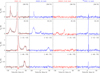 |
Fig. A.1 Spectra of the four transitions observed with ALMA convolved to an angular resolution of 11″ to simulate an observation with the IRAM 30m telescope. For CO(2–1), the black lines represent actual IRAM 30m observations from Tafalla et al. (2004). We note how the ALMA data recover all the CO(2–1) single-dish flux in the EHV regime (|V − V0| > 30 km s−1, where V0 = 6.7 km s−1 is the cloud systemic velocity), but lose some flux within 10 km s−1 of the ambient cloud. The offsets given in the top right corners are in arcseconds with respect to the position of IRAS 04166. |
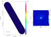 |
Fig. A.2 Maps of the 232 GHz continuum emission toward the IRAS 04166 outflow. Left: Full view of the ALMA mosaic showing a single point-like source coincident with the IRAS position. Right: Expanded view of the central 20″ × 20″ (red box in the left panel) with a stretched scale to emphasize the presence of sidelobes indicative of missing extended emission surrounding the unresolved central source. All intensities are in Jy beam−1. |
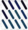 |
Fig. A.3 Maps of integrated intensity for the additional transitions observed with ALMA integrated over the EHV and SHV regimes. The coordinates and velocity ranges are as in Fig. 1. For each panel, the intensity scale is linear with limits adjusted to show maximum contrast. We note the weaker signal compared to the CO(2–1) emission. |
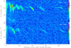 |
Fig. A.4 Position–velocity diagrams of the SiO(5–4) emission along the axis of the blue (top) and red (bottom) lobes of the IRAS 04166 outflow. The labels and scales are as in Fig. 5 |
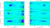 |
Fig. A.5 Position–velocity diagrams of the CO(2–1) emission perpendicular to the blue and red lobes of the IRAS 04166 outflow at 20″, 30″, and 40″ from the protostar. The weak emission inside the lobes hints at the presence of elliptical cavities indicative of nested outflow shells. |
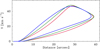 |
Fig. A.6 Position–velocity diagrams for single-event ejection models using three different density laws: r−2 (blue), r−1 (green), and no radial gradient (red). For easier comparison, all models have the same density at r = 4″. We note the similar shape of the diagrams and their overlap toward the top right region corresponding to the EHV component. This similarity indicates that the choice of density gradient has a minimal effect in the determination of the ejection model presented in Sect. 4.3. We also note that the steeper the gradient, the faster the gas moves along the PV fingers. This is a consequence of the lower density of the flow material encountered by the ejection. All models assume an inclination angle of 47° with respect to the line of sight, which corresponds to our preferred choice for the IRAS 04166 outflow (see text). |
All Figures
|
Fig. 1 Maps of the CO(2–1) intensity integrated over the EHV and SHV velocity regimes. The velocity ranges of integration are given inside square brackets and are measured with respect to a cloud LSR velocity of 6.7 km s−1. The map coordinates are offsets measured with respect to the position of IRAS 04166, and the color intensity scales at the top are in units of K km s−1. We note the different geometry of the SHV and EHV components. |
| In the text | |
|
Fig. 2 Maps of the combined blueshifted and redshifted EHV emission of CO(2–1), SiO(5–4), and SO(6,5–5,4) toward the inner 25″ × 25″ of the IRAS 04166 outflow. For CO(2–1) and SiO(5–4), the first contour and contour interval are 9 K km s−1, while for the weaker SO(6,5–5,4) they are 3 K km s−1. The map offsets are referred to the position of IRAS 04166. |
| In the text | |
|
Fig. 3 Maps of CO(2–1) intensity integrated over 8 km s−1 intervals to illustrate the different velocity regimes of the IRAS 04166 outflow. For easier comparison, the maps of blueshifted emission (top) have been rotated clockwise by |
| In the text | |
|
Fig. 4 Maps of the absolute value of the velocity centroid of CO(2–1) for the SHV (left) and EHV (right) regimes. IRAS 04166 is located at the origin of coordinates, and the color scales at the top are in units of km s−1. We note the shear pattern in the SHV regime and the velocity oscillations along the outflow axis in the EHV regime. |
| In the text | |
|
Fig. 5 Position–velocity diagrams of the CO(2–1) emission along the axis of the blue (top) and red (bottom) lobes of the IRAS 04166 outflow. The black arrows indicate some of the finger-like features that connect the EHV emission with the origin of the diagram. The velocity scale is measured in absolute value with respect to the cloud LSR velocity (6.7 km s−1), and the wedge scales on the right are in units of K. |
| In the text | |
|
Fig. 6 Left: geometry assumed for the simple model of lateral ejection from an internal working surface (IWS) presented in Sect. 4.2 (only one outflow quadrant is shown). The IWS moves along the y-axis with a constant vjet velocity and ejects gas with a vside perpendicular component. The ejected gas interacts with a surrounding shear flow and forms a shell that surrounds the jet axis (red solid curve). The plot shows the current location of the IWS (solid) and its position approximately half way along its path (dotted). The red dotted line represents the approximate trajectory between time of ejection and current time. The model predicts the expected PV diagram from an observation made at an arbitrary angle from the jet axis. Right: velocity and density profiles as a function of angle from the jet axis used to simulate the outflow shear flow. They correspond to Eqs. (1) and (2) in the text. |
| In the text | |
|
Fig. 7 Summary of results from modeling four different modes of lateral ejection from a jet. Each mode is represented by a quadrant, and is labeled with its kinematic characteristics and color-coded for easier reference. In each quadrant, the vertical diagram represents a map of the ejected gas, and two horizontal diagrams are position–velocity plots for inclinations of 90° for a jet moving in the plane of sky and 47° for expected inclination of the IRAS 04166 outflow (see text for details). |
| In the text | |
|
Fig. 8 Comparison between the PV diagram from a multi-ejection model (middle) and the ALMA observations of the IRAS 04166 outflow (as shown in Fig. 5). The intensity scale of the model is linear but arbitrary since it is simply scaled from the amount of ejected plus swept-up gas. |
| In the text | |
|
Fig. A.1 Spectra of the four transitions observed with ALMA convolved to an angular resolution of 11″ to simulate an observation with the IRAM 30m telescope. For CO(2–1), the black lines represent actual IRAM 30m observations from Tafalla et al. (2004). We note how the ALMA data recover all the CO(2–1) single-dish flux in the EHV regime (|V − V0| > 30 km s−1, where V0 = 6.7 km s−1 is the cloud systemic velocity), but lose some flux within 10 km s−1 of the ambient cloud. The offsets given in the top right corners are in arcseconds with respect to the position of IRAS 04166. |
| In the text | |
|
Fig. A.2 Maps of the 232 GHz continuum emission toward the IRAS 04166 outflow. Left: Full view of the ALMA mosaic showing a single point-like source coincident with the IRAS position. Right: Expanded view of the central 20″ × 20″ (red box in the left panel) with a stretched scale to emphasize the presence of sidelobes indicative of missing extended emission surrounding the unresolved central source. All intensities are in Jy beam−1. |
| In the text | |
|
Fig. A.3 Maps of integrated intensity for the additional transitions observed with ALMA integrated over the EHV and SHV regimes. The coordinates and velocity ranges are as in Fig. 1. For each panel, the intensity scale is linear with limits adjusted to show maximum contrast. We note the weaker signal compared to the CO(2–1) emission. |
| In the text | |
|
Fig. A.4 Position–velocity diagrams of the SiO(5–4) emission along the axis of the blue (top) and red (bottom) lobes of the IRAS 04166 outflow. The labels and scales are as in Fig. 5 |
| In the text | |
|
Fig. A.5 Position–velocity diagrams of the CO(2–1) emission perpendicular to the blue and red lobes of the IRAS 04166 outflow at 20″, 30″, and 40″ from the protostar. The weak emission inside the lobes hints at the presence of elliptical cavities indicative of nested outflow shells. |
| In the text | |
|
Fig. A.6 Position–velocity diagrams for single-event ejection models using three different density laws: r−2 (blue), r−1 (green), and no radial gradient (red). For easier comparison, all models have the same density at r = 4″. We note the similar shape of the diagrams and their overlap toward the top right region corresponding to the EHV component. This similarity indicates that the choice of density gradient has a minimal effect in the determination of the ejection model presented in Sect. 4.3. We also note that the steeper the gradient, the faster the gas moves along the PV fingers. This is a consequence of the lower density of the flow material encountered by the ejection. All models assume an inclination angle of 47° with respect to the line of sight, which corresponds to our preferred choice for the IRAS 04166 outflow (see text). |
| In the text | |
Current usage metrics show cumulative count of Article Views (full-text article views including HTML views, PDF and ePub downloads, according to the available data) and Abstracts Views on Vision4Press platform.
Data correspond to usage on the plateform after 2015. The current usage metrics is available 48-96 hours after online publication and is updated daily on week days.
Initial download of the metrics may take a while.