| Issue |
A&A
Volume 706, February 2026
|
|
|---|---|---|
| Article Number | A40 | |
| Number of page(s) | 24 | |
| Section | Extragalactic astronomy | |
| DOI | https://doi.org/10.1051/0004-6361/202555925 | |
| Published online | 29 January 2026 | |
PHANGS-JWST: The largest extragalactic molecular cloud catalog traced by polycyclic aromatic hydrocarbon emission
1
Argelander-Institut für Astronomie, University of Bonn Auf dem Hügel 71 53121 Bonn, Germany
2
Department of Astronomy, Ohio State University 180 W. 18th Ave Columbus OH 43210, USA
3
Center for Cosmology and Astroparticle Physics 191 West Woodruff Avenue Columbus OH 43210, USA
4
Dept. of Physics, 4-183 CCIS, University of Alberta Edmonton AB T6G 2E1, Canada
5
Department of Astronomy & Astrophysics, University of California, San Diego 9500 Gilman Dr. La Jolla CA 92093, USA
6
Cardiff Hub for Astrophysics Research and Technology (CHART), School of Physics & Astronomy, Cardiff University The Parade CF24 3AA Cardiff, UK
7
Department of Astronomy, Oskar Klein Center, Stockholm University, AlbaNova University Center SE-106 91 Stockholm, Sweden
8
I. Physikalisches Institut, Universität zu Köln Zülpicher Str 77 D-50937 Köln, Germany
9
Sterrenkundig Observatorium, Universiteit Gent Krijgslaan 281 S9 B-9000 Gent, Belgium
10
European Southern Observatory (ESO) Karl-Schwarzschild-Straße 2 85748 Garching, Germany
11
Universität Heidelberg, Zentrum für Astronomie, Institut für Theoretische Astrophysik Albert-Ueberle-Str. 2 69120 Heidelberg, Germany
12
Universität Heidelberg, Interdisziplinäres Zentrum für Wissenschaftliches Rechnen Im Neuenheimer Feld 205 D-69120 Heidelberg, Germany
13
Harvard-Smithsonian Center for Astrophysics 60 Garden Street Cambridge MA 02138, USA
14
Elizabeth S. and Richard M. Cashin Fellow at the Radcliffe Institute for Advanced Studies at Harvard University 10 Garden Street Cambridge MA 02138, USA
15
Department of Physics, Tamkang University, No.151, Yingzhuan Road Tamsui District New Taipei City 251301, Taiwan
16
School of Physics and Astronomy, University of, N Haugh St Andrews KY16 9SS, United Kingdom
17
Department of Physics & Astronomy, University of Wyoming Laramie WY 82071, USA
18
Department of Physics, University of Arkansas, 226 Physics Building 825 West Dickson Street Fayetteville AR 72701, USA
19
Department of Astronomy, University of Cape Town Rondebosch 7701, South Africa
20
Sub-department of Astrophysics, Department of Physics, University of Oxford Keble Road Oxford OX1 3RH, UK
21
UK ALMA Regional Centre Node, Jodrell Bank Centre for Astrophysics, Department of Physics and Astronomy, The University of Manchester Oxford Road Manchester M13 9PL, UK
22
Department of Physics and Astronomy, The Johns Hopkins University Baltimore MD 21218, USA
23
IRAP/OMP/Université de Toulouse, 9 Av. du Colonel Roche BP 44346 F-31028 Toulouse cedex 4, France
24
Space Telescope Science Institute Baltimore MD 21218, USA
★ Corresponding author: This email address is being protected from spambots. You need JavaScript enabled to view it.
Received:
12
June
2025
Accepted:
7
November
2025
Abstract
High-resolution JWST images of nearby spiral galaxies reveal polycyclic aromatic hydrocarbon (PAH) structures that potentially trace molecular clouds, even CO-dark regions. For this paper, we identified ISM cloud structures in PHANGS-JWST 7.7 μm PAH emission maps for 66 galaxies, smoothed to a common physical resolution of 30 pc and at native resolution. We extracted 108 466 cloud structures in the 30 pc sample and 146 040 clouds in the native resolution sample. We then calculated their molecular properties following a linear conversion from PAH to CO. Given the tendency for clouds in galaxy centers to overlap in velocity space, we opted to flag these clouds and omit them from the analysis in this work. The remaining clouds correspond to giant molecular clouds, such as those detected in CO(2 − 1) emission by ALMA, or lower surface density clouds that either fall below the ALMA detection limits of existing maps or genuinely have no molecular counterpart. We specifically used the homogenized sample for our analysis. Upon cross-matching the PAH clouds to the ALMA CO clouds at a homogenized resolution of 90 pc in 27 galaxies, we find that 41% of the PAH clouds are associated with a CO counterpart. We also show that the converted molecular cloud properties of the PAH clouds do not differ much when compared in different galactic environments. However, outside the central environment, the highest molecular mass surface density clouds are preferentially found in spiral arms. We further apply a lognormal fit to the mass spectra to an unprecedented extragalactic completeness limit of 2 × 10³ M⊙, and find that spiral arms contain the most massive clouds compared to other galactic environments. Our findings support the idea that spiral arm gravitational potentials foster the formation of high surface density clouds, and that lower surface density clouds form in the interarm regions. The cloud Σmol values show a decline of a factor of ∼1.5 − 2 toward the outer 2 − 3 Re. However, the trend largely varies in individual galaxies, with flat, decreasing, and even no trend as a function of Rgal. Factors such as large-scale processes, galaxy types, and morphologies might influence the observed trends. We note that combining homogenized molecular properties of individual galaxies leads to the loss of information about the physical processes that are driving deviations in trends of those properties across different galactic environments. We published two catalogs at the CDS, one at the common resolution of 30 pc and another at the native resolution. We expect them to have broad utility for future studies of PAH clouds, molecular clouds, and star formation.
Key words: ISM: clouds / ISM: molecules / ISM: structure / galaxies: evolution / galaxies: ISM / galaxies: star formation
© The Authors 2026
 Open Access article, published by EDP Sciences, under the terms of the Creative Commons Attribution License (https://creativecommons.org/licenses/by/4.0), which permits unrestricted use, distribution, and reproduction in any medium, provided the original work is properly cited.
This article is published in open access under the Subscribe to Open model. This email address is being protected from spambots. You need JavaScript enabled to view it. to support open access publication.
1. Introduction
Giant molecular clouds (GMCs) and the stars they produce are fundamental components in the formation and evolution of galaxies. The physical characteristics and development of GMCs are closely intertwined with the larger-scale processes that shape galaxies. The conditions within the interstellar medium (ISM) significantly influence how GMCs emerge and evolve, with clear correlations observed between galactic properties and those of the clouds themselves, including gas pressure, surface density, and volume density (e.g., Colombo et al. 2014; Sun et al. 2018; Chevance et al. 2020). Since star formation predominantly takes place within the cold, dense molecular phase of the ISM, characterizing GMCs is crucial for understanding the mechanisms that set those properties and ultimately for understanding the mechanisms that drive stellar birth, and by extension, galaxy evolution (Bigiel et al. 2008; Schruba et al. 2011).
Over the past few decades, radio, millimeter, and infrared telescopes have advanced to achieve increasingly high resolution in the Milky Way and nearby galaxies, allowing us to resolve molecular clouds. With the successful launch of the James Webb Space Telescope (JWST), parsec-scale near- and mid-infrared imaging is now possible in nearby galaxies (e.g., distances < 20 Mpc). The Physics at High Angular Resolution in Nearby GalaxieS (PHANGS) survey (Leroy et al. 2021; Lee et al. 2023; Williams et al. 2024) has taken advantage of these advances in resolution to probe dust emission, specifically polycyclic aromatic hydrocarbons (PAHs), in galaxies at unprecedented sub-GMC scales of 5–30 pc.
Several techniques are available to uncover the structures and properties of molecular clouds (e.g., gas mass, surface densities, velocity dispersion, radius). The CO emission, particularly from low-J transitions such as CO(1–0) and CO(2–1), is the most traditional tracer of molecular hydrogen, benefiting from extensive calibration of metallicity, gas surface density, and others (e.g., Solomon et al. 1987; Fukui et al. 2001; Bolatto et al. 2008, 2013; Heyer et al. 2009; Fukui & Kawamura 2010; Sun et al. 2020a; Schinnerer & Leroy 2024). Cloud properties are often extracted from CO data using algorithms such as CPROPS (Rosolowsky & Leroy 2006; Rosolowsky et al. 2021), CLUMPFIND (Williams et al. 1994; Rosolowsky & Blitz 2005), and Spectral Clustering for Molecular Emission Segmentation (SCIMES; Colombo et al. 2015), enabling the identification and characterization of GMCs across nearby galaxies, especially with high-resolution CO observations from the Atacama Large Millimeter Array (ALMA), specifically PHANGS-ALMA (e.g., Leroy et al. 2021; Rosolowsky et al. 2021; Sun et al. 2022). Other methods include characterizing the intensity field of CO at fixed resolution (e.g., Hughes et al. 2013; Leroy et al. 2016; Sun et al. 2022), which recovers similar information to object-finding decomposition approaches. Dust has also long been used to trace gas, starting from star count methods and extinction mapping (e.g., Savage et al. 1977; Bohlin et al. 1978; Savage & Mathis 1979), offering an independent avenue to infer gas column densities. Recent advances using high-resolution optical imaging, such as Hubble Space Telescope (HST) observations, have enabled the derivation of sub-GMC high-resolution dust extinction maps across nearby galaxies, assuming a constant dust-to-gas ratio (e.g., Faustino Vieira et al. 2023, 2024, 2025).
Polycyclic aromatic hydrocarbons have emerged as a promising gas tracer thanks to the Spitzer Space telescope (Houck et al. 2004) and the wide sky coverage provided by WISE (Wright et al. 2010). Studies using Spitzer have shown that, in nearby galaxies, PAH emission correlates with molecular gas on spatial scales ranging from several hundred parsecs to kiloparsecs (e.g., Regan et al. 2006; Cortzen et al. 2018; Gao et al. 2019; Chown et al. 2020; Gao et al. 2022). Fortunately, the recent deployment of JWST opens a promising path forward. Its high-resolution and high-sensitivity imaging of mid-infrared PAH emission, which shows a strong correlation with CO emission (e.g., Leroy et al. 2023b; Sandstrom et al. 2023; Chown et al. 2025), provides valuable insight into this topic. This offers the prospect to use the PAH emission to measure the structure of the cold ISM at high resolution and sensitivity (e.g., Leroy et al. 2023b; Sandstrom et al. 2023; Meidt et al. 2023; Thilker et al. 2023; Whitcomb et al. 2023; Chown et al. 2025). Beyond the nearby Universe, JWST has also shown that the PAH–CO correspondence remains strong at intermediate- to high-redshift galaxies (e.g., Shivaei & Boogaard 2024).
Recent observations using JWST show that PAH emission can be decomposed into a first component tracing the molecular gas, where gas and dust column density variations dominate, and a second component tracing star formation, where interstellar radiation field intensity variations dominate (Leroy et al. 2023b). This result further offers new insights into the gas and dust structure at sub-GMC scales. Chown et al. (2025) expanded this study to all PHANGS-JWST galaxies and further showed an excellent correspondence between the different JWST MIRI filters, specifically the F770W, and CO emission. They further suggested that PAH emission maps could be effectively converted to CO maps to obtain a more sensitive version than the already existing ALMA maps. However, JWST observations have further highlighted how PAH emission behaves differently in different environments. For instance, in active galactic nucleus (AGN) environments, PAHs can be partially destroyed or their emission suppressed due to strong radiation fields and shocks, whereas in star-forming galaxies without AGN activity, they remain a robust tracer of molecular material (e.g., García-Bernete et al. 2022, 2024).
An important advantage of PAH emission is its ability to trace low-density regions where CO is faint or absent. Unlike CO, which requires sufficient shielding to avoid photodissociation (e.g., Bolatto et al. 2013; Saintonge & Catinella 2022), PAHs can emit in diffuse UV-irradiated environments. This allows PAH emission to probe the full extent of molecular cloud complexes, including CO-“dark” molecular gas components (e.g., Leroy et al. 2023a; Sandstrom et al. 2023). It is important to note, however, that the F770W filter also traces emission from hot dust continuum, stellar continuum, and weak ionic or molecular lines (e.g., Draine & Li 2007; Whitcomb et al. 2023).
Sun et al. (2022) (see also Sun et al. 2018, 2020a,b; Rosolowsky et al. 2021) analyzed the PHANGS-ALMA galaxy sample, examining molecular gas properties across different galactic environments at a fixed physical resolution of 60–150 pc. Their results suggest that kiloparsec-scale environmental conditions largely drive variations in cloud populations from galaxy to galaxy. They also find that cloud-scale surface densities, velocity dispersions, and turbulent pressures increase toward galactic centers, reaching exceptionally high values in the centers of barred galaxies, where the gas also appears to be less gravitationally bound, and are moderately elevated in spiral arms compared to interarm regions. However, the homogenized resolution for the full PHANGS-ALMA sample is 150 pc. Fortunately, with PHANGS-JWST, images resemble sharper, more sensitive versions of ALMA CO maps for the same galaxies. The resolution is also enhanced by a factor of five (homogenized resolution of 30 pc) for the F770W band. This means that fainter and smaller structures can now be investigated and might be associated with either molecular clouds or the atomic phase of the ISM (see Sandstrom et al. 2023; Leroy et al. 2023b).
Several other observations surveys investigated such properties of clouds in the Milky Way (e.g., Roman-Duval et al. 2010; Eden et al. 2012; Duarte-Cabral et al. 2020) and nearby galaxies (e.g., Hirota et al. 2011; Rebolledo et al. 2012, 2015; Colombo et al. 2014; Usero et al. 2015; Rosolowsky et al. 2021). Some suggest that their star formation rates and/or efficiencies (e.g., Rebolledo et al. 2012, 2015) and mass distributions (e.g., Colombo et al. 2014) differ, for instance due to their crossing through spiral arms (e.g., Duarte-Cabral & Dobbs 2017), and that the most massive clouds are mostly found in the spiral arms (e.g., Rebolledo et al. 2012; Faustino Vieira et al. 2024). This difference could be due to self gravity in the spiral arms, agglomeration of pre-existing molecular clouds (e.g., Field & Saslaw 1965; Taff & Savedoff 1972; Scoville & Hersh 1979; Casoli & Combes 1982; Dobbs 2008), shock compression driven by spiral structures (e.g., Meidt et al. 2013), or due to low shear effects (e.g., Elmegreen 2011) or other factors. Other authors have measured cloud mass spectra that are uniform and independent of the physical conditions in their surroundings (e.g., Eden et al. 2012; Meyer et al. 2013).
Simulations have also investigated GMCs and their evolution across different environments (e.g., Dobbs et al. 2006; Nimori et al. 2012; Fujimoto et al. 2014; Dobbs 2015; Duarte-Cabral & Dobbs 2016; Grand et al. 2017; Hopkins et al. 2018; Treß et al. 2021; Smith et al. 2020; Colman et al. 2024). Duarte-Cabral & Dobbs (2016, 2017) found that most clouds exhibit properties largely independent of their location within the galaxy. However, some tails of the distributions depend on their location, indicating that more extreme clouds favor specific environments. In addition, Pettitt et al. (2020) investigated different spiral arm models and saw differences in the interarm–arm mass spectra. Furthermore, analytical and numerical approaches suggest that the GMC lifecycle varies with the galactic environment (e.g., Dobbs & Pringle 2013; Fujimoto et al. 2014; Dobbs et al. 2014; Jeffreson & Kruijssen 2018; Meidt et al. 2018).
For this paper, we identified PAH clouds in 66 homogenized 7.7 μm emission PHANGS-JWST Cycle 1 (Lee et al. 2023; Williams et al. 2024) and Cycle 2 (Chown et al. 2025) galaxy maps at a fixed resolution of 30 pc. We then used a linear conversion fit to convert the dust to CO emission maps using the prescription of Chown et al. (2025). This method provides insights into molecular clouds with higher resolution than current CO surveys and offers improved sensitivity for detecting smaller and fainter structures in the ISM. We also analyzed systematic environmental effects for a statistically significant sample of nearby galaxies, and present the molecular properties of PAH-to-CO converted structure down to an unprecedented extragalactic completeness limit of ∼2 × 10³ M⊙ which is 2.4 dex better than the previous ALMA-based CO approach (e.g., Rosolowsky et al. 2021).
The layout of the paper is as follows. In Sect. 2 we describe the data used in the study. In Sect. 3 we briefly explain the cloud extraction algorithm, SCIMES, and its input parameters. In Sect. 4 we detail the different cloud properties and how we derived them. In Sect. 5 we describe the distribution of identified structures and their properties as a function of different galactic environments, while highlighting the caveats of our approach. Finally, in Sect. 6 we summarize our findings and present our conclusions.
2. Data and galaxy sample
We used a subset of 66 galaxies with high-resolution PHANGS-ALMA CO(2 − 1) and JWST imaging tracing the PAH emission (see Table B.1). The galaxies are star-forming and have specific star formation rates (SFR/M★)≳10−11 yr−1, stellar masses (M★)≳109.5 M⊙ and CO luminosities (LCO) 6.60 < log10(LCO [K km s−1]) < 9.50, have moderate inclination (i ≲ 70°), and are at distances (D) ≲ 20 Mpc (Leroy et al. 2021).
2.1. JWST mid-IR data
JWST MIRI filters provide high angular resolution and sensitivity imaging of dust emission maps, achieving sub-GMC scales in nearby galaxies. The full width at half maximum (FWHM) is 0.269″, 0.328″, 0.375″, and 0.674″ for the F770W, F1000W, F1130W, and F2100W bands, respectively. Generally, those wavelengths capture stochastic emission from dust grains, including PAHs. Strong PAH features can be traced using the 7.7 μm band (C–C stretching modes of PAHs) which are mainly due to ionized PAHs for a range of sizes, and 11.3 μm band (C–H out-of-plane bending modes of PAHs) due to mostly larger and neutral PAHs. The 10 μm band captures a mix of PAH and continuum emission, in addition to silicate features and prominent emission lines, while the 21 μm band traces only continuum emission (Draine & Li 2007; Spoon et al. 2006; Smith et al. 2007; Tielens 2008).
We used JWST MIRI and NIRCam imaging of all 19 galaxies from the PHANGS-JWST Cycle 1 Treasury (GO 2107, PI: J. Lee; Lee et al. 2023) and 47 galaxies (available at the time of analysis, out of the full set of 51) from the PHANGS-JWST Cycle 2 Treasury (GO 3707, PI: A. Leroy; see Chown et al. 2025). Observations, data reduction, and processing using the different JWST-MIRI bands are represented in Lee et al. (2023), Williams et al. (2024), and Chown et al. (2025).
For the analysis presented in this paper, we used the F770W band to take advantage of the highest resolution MIRI band that captures PAH emission. The median physical resolution is ∼20 pc for the full sample with a 16 − 84% range of 15 − 25 pc. Given that the Rayleigh-Jeans tail of the stellar distribution contributes to the F770W band, it needs to be subtracted from the total surface brightness to obtain the emission from PAHs alone. In our analysis, we used stellar-continuum-subtracted F770W images obtained by subtracting the F200W (Cycle 1) or F300M (Cycle 2) times a scaling factor from the F770W filter following Sutter et al. (2024). The F770W stellar continuum correction (F770W★) = 0.22 × F300M for Cycle 2, or 0.12 × F200W for Cycle 1. Additionally, we leverage empirical scaling relations that relate CO emission to the continuum-subtracted F770W maps. The dust continuum contribution might have a significant contribution to the F770W band. Whitcomb et al. (2023) and Dale et al. (2025) applied a method based on Spitzer Space Telescope mid-infrared spectra of nearby star-forming galaxies coupled with synthetic F770W, F1000W, and F1130W photometry (see Whitcomb et al. 2023 and Hands et al., in prep.). They find that the continuum-free PAH emission is ∼83%. We further apply this method and find that across the Cycle 1 targets, the continuum-free PAH contribution is ∼81%. However, there are regions within the galaxies, particularly around HII regions and toward the centers, where the PAH contribution decreases further, consistent with the known suppression of PAHs in these environments. In the central regions, the contribution can reach values of roughly ∼20% or lower on average (for more details, see Hands et al., in prep.).
To be able to make a comparison of the 66 galaxies in the sample at the same physical resolution, we smoothed our data to a common physical resolution of ∼30 pc. This corresponds to the MIRI F770W resolution for the farthest galaxy in our sample (NGC 3507). We used JWST point spread functions (PSFs) generated by webbpsf1. We then created a convolution kernel per galaxy per filter using jwst_kernels2 to achieve the required physical resolution. Finally, following Williams et al. (2024), we convolved our data and error maps using our corresponding convolution kernel. For our analysis, we used this common resolution sample. We also provide a catalog constructed at the native angular resolution of each map.
2.2. Converting 7.7 micron to CO
The emission from PAHs shows a close link with CO emission on kiloparsec and parsec scales, revealing a strong correlation between both emissions over three orders of magnitude of intensity (Regan et al. 2004; Gao et al. 2019; Chown et al. 2020; Leroy et al. 2021, 2023a,b; Whitcomb et al. 2023; Chown et al. 2025). Following Chown et al. (2025), to first order, we expect
 (1)
(1)
where IPAH and ICO are the observed intensities of PAH and CO emission in MJy sr−1 and K km s−1, respectively. The dust-to-gas mass ratio is DGR, qPAH is the PAH-to-dust mass fraction, U is the strength of the interstellar radiation field relative to that in the Solar neighborhood (qPAH and U are defined in Draine & Li 2007), and XCO is the CO-to-H2 conversion factor.
Chown et al. (2025) also analyzed the resolved correlation between CO and the different PAH emission bands in 70 PHANGS galaxies, of which 66 are used here. They found the following relation
 (2)
(2)
with scatter σ = 0.43 dex. IF770W is the nonstellar continuum subtracted intensity and IF770W★ is the stellar continuum correction which comes from NIRCAM, following the relations presented in Section 2.1, and CF770WPAH is the normalization of the best-fit CO(2 − 1) versus F770WPAH power law for each galaxy (see Equation (4) in Chown et al. 2025). This normalization aims to remove the galaxy-to-galaxy scatter in the relationship. We relied on the CF770WPAH values provided by Table 3 in Chown et al. (2025). We note that this PAH-to-CO fit underestimates the CO emission in some galaxies (see Chown et al. 2025), and the place where it most prominently breaks is in galaxy centers, which show an offset relation. Equation (2) also does not correct for dust continuum emission, which might also have more prominent contributions toward central regions. However, since we directly use the galaxy intensity maps that the equation was calibrated for, we do not particularly care if the emission is due to PAHs or small dust grains. Thus, we do not do any dust continuum corrections and acknowledge that toward the central regions, we are tracing emission of PAHs with a significant contribution from the dust continuum.
The emission from PAHs could also emerge from dust mixed with atomic gas (Sandstrom et al. 2023). Hence, the relation between CO and PAHs is only used in regions where the inclination-corrected IF770WPAH ≥ 1 MJy sr−1 and where the molecular mass surface density (Σmol) ≳ 4 M⊙ pc−2 (see Leroy et al. 2023a; Chown et al. 2025, for further explanation).
Dust also exists in regions where CO is dark, typically the outer layers of molecular clouds where CO is photodissociated by ultraviolet radiation into ionized carbon (C II) (e.g., Wolfire et al. 2010; Glover & Smith 2016). These regions still contain H2, which survives due to effective self-shielding and the presence of dust (van Dishoeck & Black 1988). Dust is also present in low-metallicity environments, where the reduced dust-to-gas ratio and lower carbon abundance limit the formation and survival of CO, causing it to trace only a small fraction of the total H2 mass (Leroy et al. 2011; Bolatto et al. 2008; Smith et al. 2014). Since the conversion from PAH to CO is applied to regions regardless of whether CO exists, the converted intensity might also trace CO-dark regions.
2.3. Environmental masks
A key part of this work involves studying the properties of the (giant) molecular clouds with respect to the galactic environment. To categorize the galactic environment of each GMC, we employed the PHANGS environmental masks developed by Querejeta et al. (2021). These masks were created using the 3.6 μm Spitzer Survey of Stellar Structures in Galaxies (S4G; Sheth et al. 2010) along with other Near Infrared (NIR) observations. This approach produced detailed morphological masks of subgalactic environments for galaxies within the PHANGS survey. Notably, these masks are purely morphological and do not include kinematic information, which might lead to alternative definitions of the environments.
For our study, we employ those simple masks to categorize the galactic environments into the following regions: center, which denotes the small bulge or nucleus; bar, encompassing the bar feature along with its ends (and any overlap with spiral arms); spiral arm, extending from the interbar region to the full extent of the spiral structure; interarm, covering the space between the bar and the spiral arms as well as in-between spiral arms, and the outer disk in galaxies lacking distinct spiral features or masks; and disk, which includes the region outside the bar.
3. SCIMES cloud extraction
To identify GMCs, we adopted a machine learning algorithm called SCIMES3 (Colombo et al. 2015, hereafter C15, see also Colombo et al. 2019, and Appendix A for information about the updated version of the algorithm). This method considers the dendrogram of the emission in the framework of graph theory and utilizes spectral clustering to find regions with similar emission properties. Various other segmentation methods exist, from simple brightness thresholding (Sanders & Mirabel 1985; Solomon et al. 1987; Dame et al. 2001) to more sophisticated approaches that identify characteristic geometries (GAUSSCLUMPS, Stutzki & Guesten 1990), or associate neighboring voxels by their values (Clumpfind and CPROPS, Williams et al. 1994; Rosolowsky & Leroy 2006; Rosolowsky et al. 2021).
As described in C15, SCIMES classifies molecular clouds by first identifying dendrogram structures and then constructing a similarity (or affinity) matrix based on selected properties, which in this study are Mmol and radius. Next, SCIMES computes the spectral embedding, applies the k-means algorithm, and determines the optimal clustering configuration for each galaxy. The parameters used to build the dendrograms using the IF770WPAH maps of 66 galaxies and run SCIMES on this galaxy sample are described below.
3.1. Dendrogram structures
Dendrograms represent hierarchical structures within intensity maps, where emission regions are nested at different intensity levels. In this context, they provide a tree-like representation of cloud substructures based on spatial (position-position) information in two-dimensional data or spatial and spectral (position-position-velocity) information in three-dimensional data cubes. They are tree-like structures composed of leaves, branches, and trunks. Following the definition of Houlahan & Scalo (1992), the leaves are the local maxima in the data; they are on top of the dendrogram and have no substructure. On the other hand, the branches can contain multiple substructures and split into other branches and leaves. A third structure, the trunk, is the largest structure with no parent structure, and represents the base of the dendrogram where all the branches and leaves eventually merge (i.e., the lowest contour level).
The local maxima in this publication refer to the position-position (PP) maxima in IF770WPAH maps at a homogenized resolution of 30 pc. The structures that are due to noise are suppressed by ensuring that only emission above a given threshold (min_value, typically taken to be a multiple of the noise rms) is considered in constructing the dendrogram, and that local maxima are eliminated if they cover an area lower than a certain number of pixels (min_npix, usually limited by the spatial resolution), or if its local maximum value is lower than a certain flux difference (min_delta, also refers to the step size for the intensity levels, usually set as a multiple of the noise) above the level at which that maximum merges with another local maximum. SCIMES uses the dendrogram implementations from Rosolowsky et al. (2008). The dendrogram and catalog of the structures within SCIMES are constructed using the Python package Astrodendro4 It requires four parameters as input: data, which is the data cube or in our case the IF770WPAH map; min_value, in our case this is set to be the three times the worst sensitivity level of the data, σrms, to make sure that our structures are significant; min_delta, also set to be three times the sensitivity level; min_npix, set to be the number of pixels per beam (Ωbeam/Ωpix, where Ωbeam and Ωpix are the solid angles of the resolution element and the pixel, respectively). We use a common σrms input for all 66 galaxies, which refers to the maximum σrms value of our sample (3σrms ∼ 0.19 MJy sr−1 ∼ 0.21 K km s−1 as per Eq. (2)).
3.2. SCIMES
The SCIMES algorithm deploys spectral embedding and clustering techniques to enhance the identification of molecular clouds within a dendrogram. This approach leverages the properties of the graph Laplacian to map data into a space where clustering properties are more pronounced, followed by clustering in this transformed space using the k-means algorithm.
We used the SpectralCloudstering class in SCIMES, which deals with embedding, clustering, and choosing the best clustering configuration. This class takes different input parameters, some crucial ones are dendrogram, which is the dendrogram structure of the data generated by Astrodendro; catalog, the catalog that contains property (e.g., flux, radius) information of each structure created by the dendrogram; header, corresponding to the header of the data FITS file; criteria, that specifies which affinity matrix criteria to be used and can use multiple criteria (e.g., flux, radius, volume); user_scalpars, which is an optional scaling parameter that can be used to Gaussian smooth the affinity matrix. It should be noted that each affinity criterion has an associated scaling parameter that can be set. We also set save_all = True, which retains discarded structures, including both isolated leaves and intra-clustered leaves that are typically removed as noise. This ensures that small PAH cloud structures, which may still hold physical significance, are preserved in the final catalog. Additionally, this setting retains unassigned branches within clusters, allowing a more complete representation of the cloud hierarchy.
For our study, we used the molecular mass (see Sect. 4.2) and radius of the structures as the clustering affinity criteria, and the pp_catalog function from Astrodendro to create the catalog. We also manually set the scaling parameters to 100 pc for the radius (roughly the sizes of large GMCs; e.g., Rosolowsky et al. 2021; Demachi et al. 2024), and consistent with Faustino Vieira et al. (2025). We also set the molecular mass scaling parameter to 5 × 10⁶ M⊙ (within the upper limit of a GMC; e.g., Demachi et al. 2024). Manually setting the scaling parameters is crucial in spectral clustering, as this scaling parameter essentially determines the weighting of radius and mass when computing similarities between clouds, and removes structures that show affinity connections on scales larger than typical GMC scales (see Appendix D.6 for details on our choice of scaling parameters).
4. Molecular cloud properties
In this section, we present the different methods used to calculate the sizes and fluxes of the clouds identified by SCIMES. We directly infer the radius based on the exact footprint area of the cloud (e.g., Williams et al. 1994; Heyer et al. 2001), and following Rosolowsky & Leroy (2006) (hereafter R06), we also use moment measurements to compare our findings to results from CO-based GMC catalogs for the same PHANGS galaxies (Hughes et al., in prep.).
4.1. Directly measured properties
One direct way of finding the radius of a structure is by directly inferring it from the area (e.g., Williams et al. 1994; Heyer et al. 2001). Consider a cloud with N pixels; then the area of the cloud is simply
 (3)
(3)
where Apix represents the pixel area. Subsequently, the deconvolved equivalent radius of the cloud can be found as
 (4)
(4)
where ![Mathematical equation: $ A_{\mathrm{beam}}\,[\mathrm{pc}^{2}] = 1.18^{2} \sigma_{\mathrm{b,maj}}\,[\mathrm{deg}]\sigma_{\mathrm{b,min}}\,[\mathrm{deg}]\left(\frac{\pi \times D\,[\mathrm{pc}]}{180}\right)^{2} $](/articles/aa/full_html/2026/02/aa55925-25/aa55925-25-eq5.gif) is the beam area of the observation, and σb, maj and σb, min are the beam major and minor axes expressed in degrees (see Appendix D.7 for more information).
is the beam area of the observation, and σb, maj and σb, min are the beam major and minor axes expressed in degrees (see Appendix D.7 for more information).
Following R06, the radius of the cloud can also be assessed by intensity-weighted moment-based measurements
 (5)
(5)
where η depends on the light distribution within the cloud (see R06). In this paper, we use a value of  corresponding to the half-width at half-maximum of a Gaussian distribution (e.g., Rosolowsky et al. 2021). The size of the cloud is σr, and σmaj and σmin are the second spatial moments (see R06 for further information).
We converted the IF770WPAH to ICO(2 − 1) (see Sect. 2.2) and obtained the converted luminosity in CO of a cloud, which can then be defined as
 (6)
(6)
Fi represents here the flux in units of K km s−1 of an element in the cloud obtained from Eq. (2), and it is summed over all cloud pixels. Apix is the projected physical area of the pixel in units of pc2.
4.2. Derived physical properties
In this section, we present the physical properties that we derived from either the moments method or the direct estimation of the radius from the beam-deconvolved area of the cloud. The radii of the clouds are converted from arcsec to parsec using D measurements from Table 3 in Leroy et al. (2021).
After converting IF770WPAH to ICO(2 − 1) following Eq. (2), the molecular mass of CO can be derived from the luminosity (Eq. (6)) as
![Mathematical equation: $$ \begin{aligned} \mathrm M_{\rm mol} \,[\mathrm M_{\odot } ] = \alpha _{\rm CO}\,[\mathrm M_{\odot }(K\,km\,s^{-1}\,pc^{2})^{-1} ] \times L_{\rm CO}\,[\mathrm K\,km\,s^{-1}\,pc^{2} ], \end{aligned} $$](/articles/aa/full_html/2026/02/aa55925-25/aa55925-25-eq9.gif) (7)
(7)
where αCO (and previously defined XCO) refer to the CO-to-H2 conversion factor (see Bolatto et al. 2013 for detailed definition). For each identified cloud, we take a median αCO value within its boundary, and then multiply it by the LCO of the cloud to obtain Mmol.
In the case of PHANGS-ALMA, the CO transition observed is CO(2 − 1), thus, we refer to the conversion factor as αCO(2 − 1). We also rely on an updated version of the PHANGS-ALMA αCO(2 − 1) estimates presented by Sun et al. (in prep.) (see also Sun et al. 2022, 2023), based on the recommended αCO from Schinnerer & Leroy (2024), which incorporates corrections for excitation, CO-dark gas, and emissivity variations. Following Schinnerer & Leroy (2024), we define αCO(2 − 1) as:
 (8)
(8)
where f(Z) = (Z/Zsolar)−1.5 is the CO-dark factor that depends on the metallicity (Z) for 0.2 < Z/Zsolar < 2 (see Schinnerer & Leroy 2024 for further information), where Zsolar is the solar metallicity (12 + log(O/H) = 8.69 as per Asplund et al. 2009). This prescription complements observations of dust and C II, where a higher αCO is needed in regions of low mass and low metallicity (e.g., Leroy et al. 2011; Jameson et al. 2016). It is also an accompaniment to simulations which reveal a strong dependence of αCO on metallicity, with significantly suppressed CO emission at low metallicity and low extinction (e.g., Glover & Low 2011; Hu et al. 2022). However, f(Z) does not take into consideration additional factors such as the dust-to-metals ratio, interstellar radiation field, cosmic ray ionization rate, and the structure of the clouds themselves, which all play an important role, and further add to the uncertainty of the Mmol estimation. The starburst emissivity factor is g(Σ★) = max(Σ★/100, 1)−0.25, where Σ★ is the stellar mass surface density in units of M⊙ pc−2. Additionally, R21(ΣSFR) is the line ratio between CO(2 − 1) and CO(1 − 0), and ΣSFR is the star formation rate surface density (see Leroy et al. 2022 and Schinnerer & Leroy 2024 for more information). The metallicity is approximated as a function of galactocentric radius based on the global mass-metallicity relation of Sánchez et al. (2019), adopting the PP04 O3N2 calibration (Pettini & Pagel 2004) and extrapolating the predictions to the whole PHANGS-ALMA footprint using a metallicity gradient as per Sánchez et al. (2014) (see Sun et al., in prep., for more information).
We then calculate the molecular mass surface density as follows
![Mathematical equation: $$ \begin{aligned} \Sigma _{\rm mol}\,[\mathrm{M}_{\odot }\,\mathrm{pc}^{-2}]&= \frac{\mathrm{M}_{\mathrm{mol}}}{{\pi } \mathrm{R}_{\mathrm{eq}}^{2}},\end{aligned} $$](/articles/aa/full_html/2026/02/aa55925-25/aa55925-25-eq11.gif) (9)
(9)
![Mathematical equation: $$ \begin{aligned} \Sigma _{\rm mol,R}\,[\mathrm M_{\odot }\,\mathrm{pc}^{-2}]&= \frac{\mathrm{M}_{\mathrm{mol}}}{2\pi \mathrm{R}^{2}}\cdot \end{aligned} $$](/articles/aa/full_html/2026/02/aa55925-25/aa55925-25-eq12.gif) (10)
(10)
The model in Eq. (9) follows that Σmol is directly inferred from the area of the cloud. Meanwhile, the model in Eq. (10) follows the two-dimensional Gaussian cloud model in which half the mass is contained inside the FWHM. We used the first model throughout the paper and the second model only to compare PAH and CO clouds in Sect. 5.1.
4.3. Error estimation
We applied morphological alterations to the shapes of individual clouds to estimate the errors in their properties, given that many of their properties depend on the exact cloud footprint, and thus on the number of pixels assigned in the cloud segmentation process. The SCIMES-defined structures exhibit only slight variations depending on the input parameters of the dendrograms, except for min_value, where more variations are observed (Colombo et al. 2015). Varying the scaling parameters by a small fraction (∼20%) also leads to slight variations in the properties of the clouds. Therefore, to quantify the potential uncertainties in the cloud properties due to the choice of assignment mask, we used the binary_erosion and binary_dilation functions of the scipy.ndimage5 Python package. We applied a dilation and erosion with one-third the number of pixels per beam (∼10 pc) and calculated the cloud properties of both as upper and lower limits, respectively.
Following R06, we also estimate the errors for the properties of the clouds by bootstrapping. This involves generating several trial clouds from the original data by randomly sampling the data points within the cloud, with some points being repeated. A cloud in this case is considered to be a collection of data {xi, yi, Ti}, for i = 1, …, N, where N is the number of points in the cloud. We measured the properties of each trial cloud and estimated the uncertainty as the 84th − 50th and 50th − 16th percentiles of the distributions. This bootstrapping considers the errors from D, IF770WPAH, and the fit error (including the scatter) in Eq. (2).
To assess the bias in the cloud Mmol according to αCO, we use five different αCO prescriptions. The first prescription is represented in Eq. (8), and it is our preferred prescription used in the analysis. The second one is a constant Galactic  , where R21 = 0.65 is based on Leroy et al. (2013) and den Brok et al. (2020), measured at kpc scales, and αCO(1 − 0) = 4.35 M⊙ pc−2 (K km s−1)−1 is the standard Galactic value at solar metallicity (i.e., Bolatto et al. 2013). The third description is according to a varying metallicity and gas surface density αCO based on Eq. (31) in Bolatto et al. (2013). The fourth one also varies according to Eq. (2) in Teng et al. (2024), which relies on the intensity-weighted mean molecular gas velocity dispersion measured at 150 pc scale. The last prescription depends only on the metallicity (see Sun et al. 2020a). The exact creation of each αCO map is further described in Sun et al. (in prep.).
We calculate luminosity-weighted averages of both the cloud properties and their uncertainties within the FOV of all galaxies. This method is motivated by Leroy et al. (2016) (see also Sun et al. 2022), where they calculated the intensity-weighted average for clouds within an aperture encompassing several GMCs. Our bootstrapping technique yields a luminosity-weighted uncertainty average of the cloud mass measurement of ∼20% and that of the radius measurement is ∼7%. However, erosion and dilation yield a luminosity-weighted uncertainty average of ∼54% and ∼58% for the mass and radius measurements, respectively. To assess the αCO bias of our prescription (see Eq. (8)), we compare the luminosity-weighted Σmol average value using our adopted αCO with the other prescriptions. In spiral arms, interarms, and disks, the Σmol variation due to adopting another αCO prescription is on average ∼23%. Meanwhile, in bars, the variation is ∼49%, and in centers ∼125%. This highlights the uncertainty of the measurements toward the central regions of the galaxy. For the final error on the cloud properties, we apply Gaussian error propagation on the bootstrapping and morphological alteration methods, and provide the Mmol calculated using the different αCO prescriptions in our cloud catalog.
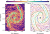 |
Fig. 1. A zoomed-in view of NGC1566, one of the 66 galaxies. Left: Continuum-subtracted intensity image of the galaxy in the F770W MIRI band. The 2σ CO intensity contours from PHANGS-ALMA are represented in black. Right: PAH cloud structures identified by SCIMES color-coded by their F770W intensities. The green, blue, and red contours indicate the spiral arm, bar, and central region masks, respectively. The interarm region in this case consists of the remaining clouds that are not enclosed by the contours. The number of PAH clouds identified in this galaxy is represented in the bottom right. The color bar at the top of the image shows the 7.7 μm intensity range of the identified clouds. |
4.4. Cloud population
Figure 1 shows an example of the PAH clouds extracted with SCIMES for one of our galaxies (NGC 1566). In this figure, we show this cloud segmentation at 30 pc resolution to show the performance of SCIMES in recognizing structures. We further provide both a common-resolution (30 pc) and sensitivity (0.19 MJy sr−1) cloud catalog, and a native resolution and sensitivity catalog.
We selected 77 884 clouds for analysis that meet our selection criteria. Initially, a total of 108 466 clouds were identified across the 66 galaxies, and all of them are included in the final cloud catalog (see information about native resolution in Appendix C). However, since we do not have velocity information, clouds with different velocities might overlap if they are along the same line of sight. For that, we used assignment cubes of GMCs identified in CO(2 − 1) from the PHANGS-ALMA survey using CPROPS (Rosolowsky et al. 2021; Hughes et al., in prep.) to check, flag, and exclude overlapping 7.7 μm-identified clouds in velocity space from our analysis. Also, we flagged and excluded clouds on the edge of the maps (f_edge = 0 to exclude in the final catalog). To ensure that most of the chosen PAH clouds are tracing the molecular phase, we only included in our analysis clouds that have an average IF770WPAH > 1 MJy sr−1 (twice the threshold suggested by Chown et al. 2025 since the 0.5 MJy sr−1 threshold still includes a significant amount of Σmol < 4 M⊙ pc−2 clouds) or Σmol > 4 M⊙ pc−2. We set a flag, f_mol = 1, to include the latter from the final catalog.
We projected the native-resolution CPROPS GMC assignment cubes onto the same grid space as the SCIMES assignment maps to exclude overlapping clouds in velocity space. Then, after applying a 2D projection of the clouds, we checked how many CO overlapping cloud pixels exist in a specific SCIMES-identified cloud. Finally, we flagged clouds that have more than 30% contribution from multiple CO clouds. In the final catalog, we include f_overlap as a binary flag, where a value of one corresponds to overlapping structure, and zero to non-overlapping ones. We also include overlap_ratio to check the ratio of overlap (e.g., a value of 0.3 corresponds to 30% overlap). Once we match those clouds with our clouds, we find that ∼12% of the full cloud sample comprises overlapping clouds. This poses a challenge in central regions as multiple velocity elements and a high-velocity dispersion exist in those regions (Rosolowsky et al. 2021); we report that ∼65% of clouds in the central regions, ∼24% bar clouds, ∼13% spiral arm clouds, ∼5% interarm clouds, and ∼12% disk clouds contain overlapping counterparts that are flagged out in the analysis.
The summary of the flagging is represented in Table 1. Also, galaxy centers have well-connected leaf structures and high branch weights in the dendrograms (i.e., extremely bright). As mentioned before, those structures are large and massive, and the central regions mainly comprise overlapping clouds in velocity. Therefore, we flag out all central clouds (1303 clouds) as explained in this section, but show them in Fig. 3 to emphasize the bias of including them.
Number of clouds excluded from our analysis using each flagging method.
In Table B.1, we show that the full cloud sample covers a median of  6, and the filtered subsample covers a median of
  of the emission from the IF770WPAH maps. This highlights that most of the flagged clouds are high Σmol clouds (> 100 M⊙ pc−2) and poses a bias in our analysis toward lower Σmol clouds.
5. Results and discussion
In this section, we investigate how well PAH-identified clouds using the F770W JWST band (see Appendix D.8 for a comparison between cloud properties extracted using the F770W and F1130W bands) could resemble CO-identified GMCs. We further rely on the common-resolution data to compare the molecular cloud properties in different galactic environments according to the Querejeta et al. (2021) environmental masks. This was previously done on the PHANGS-ALMA sample (e.g., Rosolowsky et al. 2021; Sun et al. 2022). We then present the cloud mass-radius scaling relation and mass spectrum per environment. Finally, we discuss how the cloud properties vary with respect to galactocentric radius and highlight the caveats.
5.1. IF770WPAH and CO cloud property comparison
We compare the properties of the PAH clouds identified by SCIMES at 30 pc resolution to cross-matched CO clouds identified by CPROPS at 90 pc resolution in 27 PHANGS galaxies. The galaxies in CO have a common sensitivity of 0.15 K (Rosolowsky et al. 2021; Hughes et al., in prep.). We note that CO clouds were identified using position-position-velocity (PPV) data. We find that 41% of the PAH clouds in the 27 galaxies could be associated with CO counterparts in the same FOV as JWST. We note that the completeness limit of PHANGS-ALMA is 4.7 × 10⁵ M⊙, which is ∼2.4 dex higher than our lowest Mmol clouds.
For comparison, we use Mmol measurements from the GMC catalog provided by Hughes et al. (in prep.) and based on the Schinnerer & Leroy (2024)αCO prescription (see Equation (8)). We also use second-moment measurements for the radii (as described in Sect. 4.1) for both PAH and CO clouds to maintain consistency.
The median Mmol is 8.3(±0.2)×104 M⊙ in the PAH-cloud sample; this value is one dex lower than the completeness limit of PHANGS CO-identified GMCs (Rosolowsky et al. 2021). Also, the median cloud radius is 34.7 pc. This highlights the better sensitivity and physical resolution of JWST that allows the detection of fainter and smaller clouds than CO-identified GMCs as seen in Figs. 2 and 3. However, this does not test how well PAH clouds recover CO-traced clouds. Instead, we use Σmol, R (see Eq. (10)) to compare the two cloud samples, reducing the effect of the different resolutions between the studies. We therefore compare the Σmol, R distributions of the matched CO and PAH clouds represented in Fig. 3. The median Σmol, R of the PAH clouds is 28.7 M⊙ pc−2, which is the same as that of the CO cloud sample. Also, no differences are observed in the Σmol, R distributions of both matched PAH and CO clouds in the different environments, except in the central regions. There, we notice a decrease of ∼0.3 dex in PAH-cloud Σmol, R, which introduces a caveat in our cloud identification in the central regions. This is due to the removal of overlapping clouds in velocity space from our analysis, and because the PAH-to-CO relationship most prominently breaks in galaxy centers (see Chown et al. 2025).
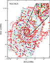 |
Fig. 2. GMCs in NGC0628. CO-identified GMCs using CPROPS are shown as red ellipses (Hughes et al., in prep.), and the 7.7 μm identified PAH clouds using SCIMES are shown in the background in different colors. A zoomed-in view of the central region is shown in the inset (upper right corner); it focuses on the structures identified by both PAH and CO. This image highlights the resolution advantage of PAH clouds and the better sensitivity compared to CO, which allows the detection of fainter and smaller clouds where CO is not detected. |
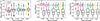 |
Fig. 3. Box plots with quantiles and outliers comparing the Σmol, R (left), cloud radius (middle), and cloud area (AR; right) distributions of cross-matched PAHs at 30 pc physical resolution and CO clouds at 90 pc in a subsample of 27 galaxies. The colored boxes represent the PAH cloud property distributions without overlapping clouds. The black boxes represent the property distributions of the cross-matched CO clouds. The dashed and dotted horizontal lines represent the median property of the full sample of CO clouds and PAH clouds, respectively. |
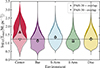 |
Fig. 4. Violin plots showing the distribution and medians of Σmol in each galactic environment for the full sample of PAH clouds (colored) and the 77 844 clouds without overlap (transparent) in the 66 galaxies. The dashed line represents the median Σmol for the full PAH cloud sample. |
5.2. Masses, radii, and surface densities
The properties of the clouds, such as Req, Mmol and Σmol analyzed in this paper are presented in Table 2. We highlight that various methods exist for calculating the properties, as outlined in Sect. 4, and these methods can produce differing results, which may impact comparisons. Therefore, caution should be taken when calculating and comparing properties with other cloud catalogs. A summary of the cloud properties listed in our catalogs can be found in Table C.1.
Summary of PAH cloud properties in various galactic environments.
The lowest and highest cloud Σmol medians are 5.8 and 49 M⊙ pc−2 corresponding to NGC 4941 and NGC 4781, respectively. This shows that the sensitivity of the IF770WPAH images allows us to locate faint structures (< 10 M⊙ pc−2; see also Sandstrom et al. 2023; Leroy et al. 2023b; Chown et al. 2025) that could be associated with atomic or molecular clouds and are not detected by ALMA observations (e.g., Rosolowsky et al. 2021). We speculate that those structures could be associated with faint clouds that CO does not detect. Notably, 51% of those clouds are located in the disk, and the rest are equally spread in the other galactic environments.
To investigate whether clouds in spiral galaxies have distinctive properties, we split our sample into “spiral” and “disk” galaxies (i.e., with and without strong spiral arms present, respectively) according to the environmental classification of Querejeta et al. (2021). We associate 30 362 clouds with 40 disk galaxies and 47 522 clouds with 26 spiral galaxies. As seen in Table 2, clouds in the spiral arm have the highest Σmol compared to other environments, followed by disk clouds, and the least dense clouds are in the interarm and bar regions (see also Fig. 4). While the PAH cloud Σmol values in bars appear similar to those of CO clouds (e.g., Fig. 3), CO emission might be systematically underestimated in bar ends across the full PHANGS–JWST sample.
When we look at the Σmol probability distribution function (PDF) of the interarm clouds in Figs. 5 and 6, we see fewer clouds with densities > 10 M⊙ pc−2 compared to spiral-arm clouds. This indicates that spiral arms favor denser clouds, which agrees with the picture proposed by Koda et al. (2009), where the potential well of the spiral arm assists in the formation of massive, dense structures. The contrast in surface densities between spiral arms and interarm is seen in the PHANGS-ALMA galaxies (e.g., Sun et al. 2020b, 2022; Meidt et al. 2021; Querejeta et al. 2024). This picture is also backed by other observations (Ragan et al. 2014) and simulations (Duarte-Cabral & Dobbs 2016, 2017; Treß et al. 2021), where they report an abundance of long filamentary objects in the interarms, and massive clouds in the spiral arms (Dobbs et al. 2011; Colombo et al. 2014).
Figures 5 and 6 reveal differences in the molecular gas distribution across galactic environments. In spiral galaxies, the number density of PAH clouds with Σmol < 10 M⊙ pc−2 is similar in spiral arm and interarm regions, and 1.2 times lower than in spiral arm compared to bar regions. In disk galaxies, cloud number densities in the disk are also 1.4 times lower than those in the bar for the same Σmol threshold. For clouds with Σmol > 10 M⊙ pc−2, spiral arms show 1.6 times higher number densities than bar regions, and 2.3 times higher than interarm regions. In this higher Σmol regime, the disk exhibits 2.1 times higher cloud number densities than bar regions. Overall, spiral arm clouds exhibit the highest number density across all Σmol values when compared to clouds in other environments (0.2 dex higher; see Table 2), and the other environments have similar cloud number densities. Additionally, disk galaxies are, on average, ∼0.5 dex less massive than spiral galaxies. Since bars tend to have a more pronounced impact on the ISM in more massive systems (e.g., Verwilghen et al. 2025), this may explain the observed similarity in the cloud Σmol distribution between bars and disks (e.g., Fig. 5) in the disk galaxies. On the other hand, Fig. 6 illustrates that the shape of the Σmol distribution is generally similar across all environments, with the exception that spiral arms host a slightly greater number of high-Σmol clouds compared to disk clouds for Σmol < 103 M⊙ pc−2, and relatively more than bar and interarm regions.
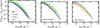 |
Fig. 5. Left: Cumulative distributions of the molecular mass surface densities from the full cloud sample. The different colors represent the different environments. The y-axis is the fraction of clouds with a surface density greater than a given value. All distributions are normalized by the total area of their specific environment, A. Middle: Same as the left plot, but only considering barred spiral galaxies and excluding disks. Right: Same as the left plot, but only considering barred disk galaxies and excluding spirals. We removed the central region from the PDFs due to overlapping cloud bias. |
 |
Fig. 6. Cumulative distributions of the molecular mass surface densities from the full cloud sample. The different colors represent the different environments. The y-axis is the fraction of clouds with a surface density greater than a given value. All distributions are normalized by the total number of clouds in their corresponding environment, Ntot. We removed the central region from the PDFs due to overlapping cloud bias. |
In the PHANGS-ALMA sample, Querejeta et al. (2021) report that, on kpc-scales, and using the Sun et al. (2020a)αCO prescription, Σmol values of interarm regions are comparable to those in disk regions, with interarm properties resembling those of disks in nonspiral galaxies (see also, Meidt et al. 2021; Querejeta et al. 2024). Expanding on this, we find that on scales of tens of parsecs, molecular clouds in the disk regions show distributions and median values of Req, Mmol, and Σmol that resemble a combination of those found in both interarm and spiral arm regions (e.g., Figs. 3 and 4). Also, using CO maps for the same galaxies presented here, previous studies (e.g., Sun et al. 2018, 2020b, 2022; Leroy et al. 2021; Querejeta et al. 2021; Leroy et al. 2025) report higher Σmol toward the central regions of galaxies, with a more pronounced increase in barred galaxies. They attribute this to bar-driven gas inflows. Here, we see a decline of Σmol in bars compared to disks. We note that toward central regions (i.e., in bars and centers), the CO emission is underestimated because the CO-to-PAH relationship is ∼0.2 dex higher there than in galactic disks (e.g., Chown et al. 2025). Also, the stellar continuum is too bright, and subtracting it becomes more difficult (e.g., Sutter et al. 2024; Baron et al. 2024). Finally, the αCO conversion factor choice does affect the measurements, especially toward central regions. The usage of an αCO that depends on Σ★, ΣSFR and the metallicity does lower the Σmol in bars and centers more than using one that does not account for all. Adopting a different αCO measurement does not affect our analysis or conclusions when comparing Σmol of clouds in spiral arms, interarms, and disks. However, when adopting another prescription, Σmol values in bars become comparable to or higher than those of galactic disks. It is worth noting that in low-metallicity regions (12+log(O/H) < 8.2), the PAH abundance, traced by the F770W/F2100W ratio drops sharply; meanwhile, at higher metallicities, the ratio reaches a plateau (Egorov et al. 2025). This highlights that PAHs could be more efficiently destroyed in the low-metallicity HII regions due to the higher UV hardness.
Finally, we divided the galaxies into active and non-active following Véron-Cetty & Véron (2010), where active galaxies are defined as quasars (starlike nuclei with broad emission lines and absolute magnitude MB < −22.25), BL Lac objects, and Seyfert galaxies (types 1–2, including LINERs), while normal galaxies are considered non-active. In our sample, 15 galaxies are classified as active. The trends in Σmol, Mmol, and Req across galactic environments are consistent between active and non-active galaxies, differing by only ∼0.1 dex. Therefore, the impact of the AGN in our sample might be small.
5.3. Cloud mass spectrum
In this section, we focus on the cloud mass spectrum, providing a more comprehensive view of the mass distribution of clouds by quantifying the fraction of clouds above or below a given threshold. This approach is motivated by previous works, such as Rosolowsky (2005) (see also Blitz et al. 2007; Fukui & Kawamura 2010; Hughes et al. 2013; Colombo et al. 2014; Mok et al. 2020). For example, Colombo et al. (2014) used mass spectra to highlight environmental differences in M51, showing steeper distributions in interarm regions than spiral arms. Similarly, cumulative and differential techniques have been used to explore the effects of feedback and dynamical processes on the molecular cloud population (Mazumdar et al. 2021) and in simulations (e.g., Colman et al. 2024). Following these methods, we employ the cloud mass spectrum to investigate the cloud population and formation. The fit itself is an important result to be matched by theories of cloud formation and evolution. By doing so, we aim to uncover how environmental factors influence the entire molecular cloud population.
Previous work has often used a single truncated or normal power law to identify the shape, steepness, or shallowness of the cloud mass spectrum (Rosolowsky 2005; Colombo et al. 2014; Mok et al. 2020). However, when analyzing a large sample of clouds, we find that they fail to catch the full distribution of clouds, especially the tail of the distribution, since it departs from a power law. Pathak et al. (2024) show that two components could represent the PDF of mid-infrared intensities in individual PHANGS-JWST Cycle 1 galaxies. A diffuse lognormal part that peaks at low intensities and strongly correlates with SFR and gas surface density, and a power law tail at high intensities that traces HII regions. The lognormal component dominates the 7.7 μm emission. Therefore, we test whether a survival function of a lognormal distribution can be used to define the mass spectra of clouds inferred from the same maps.
The lognormal distribution can be represented as
 (11)
(11)
where M (or Mmol) is the mass of the cloud. Two important parameters are the shape parameter, which refers to the standard deviation (σ), and the scale parameter (s), which refers to the eμ, where μ is the mean of the lognormal distribution.
The cumulative distribution function is
 (12)
(12)
where Φ(M) is the standard normal CDF:
![Mathematical equation: $$ \begin{aligned} \Phi (M) = \frac{1}{2} \left[ 1 + \mathrm{erf} \left( \frac{M}{\sqrt{2}} \right) \right]. \end{aligned} $$](/articles/aa/full_html/2026/02/aa55925-25/aa55925-25-eq33.gif) (13)
(13)
Here erf is the standard error function defined as  , and t is the mass element.
Therefore, the complementary cumulative distribution function (CCDF) or survival function is
 (14)
(14)
where S(M; σ, s) is the normalized form of the survival function. It should be multiplied by the total number of clouds to replicate the CCDFs shown in Fig. 7.
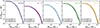 |
Fig. 7. Mass spectra for the PAH clouds in different environments, as labeled in each plot. The dashed black curves show the survival function fits. The fit parameters are displayed in the bottom left corner of each figure, where σ is the shape parameter and s is the scale parameter. The gray region represents the Poisson errors on the counts |

We rely on the CCDF description of SCIPY lognorm.sf7 package. For that, we optimize the lognormal parameters by minimizing the negative log-likelihood for the lognormal distribution using the minimize8 function in SCIPY. We apply a bootstrap of 100 iterations on the minimization to find the fit error. We fit the survival function for the full sample of clouds and per galactic environment for a completeness limit of ∼2 × 10³ M⊙ as seen in Fig. 7. This means we only consider Mmol values corresponding to more than 8 times the 3 σrms level.
We present the fit parameters in Table 3. Overall, the spiral arm and disk environments have the highest s values. The shape parameter indicates that a larger σ corresponds to a shallower distribution slope, implying the presence of more massive structures. This parameter is the highest in the spiral arm region, which, alongside the highest s value, suggests that higher-mass clouds are more prevalent in spiral arms. This trend is also evident in Fig. D.4, where the fits of individual environments closely follow each other, but spiral arm clouds have a shallower slope, appearing more prominent at higher masses.
Survival function parameters (σ, s) for the Global sample of clouds, per galactic environment, and galaxy-by-galaxy (σgal, sgal).
Furthermore, Fig. 8 shows significant scatter (∼1 dex) toward the high masses in the mass spectra. To investigate this, we compare the distributions of the individual galaxies using a Kolmogorov–Smirnov (KS) two-sample test. Of the 66 galaxies, we form 2145 pairs and check if the p-value decreases or increases when comparing the full Mmol distribution of the pairs versus the sample excluding the high-mass clouds (> 106 M⊙). In 78% of the cases, we see an increase in p-value when excluding the high-mass clouds. This indicates that the high-mass clouds are driving differences in the distributions. Figure D.4 further shows that this deviation is most prominent in the bar and disk regions. This suggests that molecular cloud formation and evolution differ more significantly between different galactic bars or disks than between different spiral arms or interarm regions.
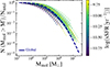 |
Fig. 8. Normalized survival function fits for PAH clouds per galaxy. The dark blue dashed line represents the global fit to the entire sample. The background thin dashed lines are color-coded by specific star formation rate (sSFR) and show the global fits to each galaxy. |
The Spearman correlation coefficient in Table 4 shows that the s of the lognormal fits reflects the median of the cloud Mmol and strongly correlates with the Σmol median. There is also a positive correlation with the sSFR (see also Figs. 8 and D.4), number density of clouds, inclination, and HI mass of the galaxy. This means that galaxies with a higher value of s tend to have more clouds within their area and more “active” star formation. Also, this reflects the nature of the PAHs tracing heating by star formation (e.g., Peeters et al. 2004; Calzetti et al. 2007; Belfiore et al. 2023; Leroy et al. 2023b). Therefore, s is a metric that mainly relates the cloud properties to their star formation capability. Additionally, the total mass within the clouds per galaxy positively correlates with the HI mass, SFR, sSFR, and the total number of clouds within the galaxy (see Table 4), indicating that star formation is more prominent in galaxies having a higher number and more massive clouds. Also, the correlation between both s and the total mass of clouds with the mass of HI hints that the atomic gas acts as a reservoir for molecular clouds, and the more atomic gas present, the more molecular clouds are forming.
Spearman correlation coefficients (r) and p-values (p) between the scale parameter of the lognormal distribution sgal, the shape parameter σgal, the total mass within clouds (∑Mmol), and various galactic and/or cloud parameters across the 66 galaxies.
To investigate how both galactic environment and host galaxy influence the variation in molecular cloud mass distributions, we compare the lognormal fit parameters obtained globally per environment (i.e., Fig. 7) with those derived on a galaxy-by-galaxy basis. The results are presented in Table 3. Across environments, the global fit parameters, particularly σ, vary in a relatively narrow range (from ∼1.37 in the disk to ∼1.53 in the spiral arms). Also, the distribution of σ values obtained from the galaxy-by-galaxy fits within each environment exhibits a similar spread. It is worth noting that the small range that σgal varies within galaxies implies that galaxies generally exhibit similar cloud Mmol PDF width, which explains why σ shows little to no correlations with the global galactic properties. Additionally, the scale parameter s, where the distribution of values from the galaxy-by-galaxy fits (with 84th to 16th percentile ranges on the order of 2 − 7 × 10⁴ M⊙) is wider than the overall shift in s across environments (ranging from ∼4 to 8 × 10⁴ M⊙). These results indicate that the differences in cloud mass distributions are not fully captured by environment-based classification alone. Instead, variation between host galaxies, even within the same environment, contributes significantly to the overall distribution.
5.4. Cloud property distributions as a function of galactocentric radius
Examining the distribution of all PAH-identified clouds as a function of galactocentric radius (Rgal) provides insight into whether local cloud properties reflect the broader structure of the gas reservoir from which they form. While large-scale processes such as gravitational torques, spiral density waves, and hydrodynamic shocks (e.g., Lin & Shu 1964; Roberts et al. 1979; Sormani & Barnes 2019; Yu et al. 2022) act on longer timescales than the lifetime of individual clouds, they significantly influence the spatial arrangement and surface density of the molecular gas. Over time, these mechanisms facilitate angular momentum loss and drive gas radially inward, giving rise to the well-known exponential decline in molecular gas surface density with radius. If cloud-scale properties such as Σmol and Req are coupled to the large-scale galactic processes, we may expect to detect systematic radial variations as a result. In this section, we investigate how Σmol and Req vary with Rgal across all 66 galaxies in our sample. PAH emission enables us to trace a broader range of cloud masses, including small clouds often missed in CO studies, allowing a more complete census of the Σmol and Req variation as a function of Rgal.
In Fig. 9, we present the radial profiles of Σmol and Req (see Eqs. (9) and (4), respectively). We further fit a Gaussian for the distribution at each radial bin and find that the Gaussian σ values are consistent between the bins. This generally indicates that the distributions span similar values in all bins. The scatter around the median is approximately 0.5–1 dex, while the individual galaxy scatter is lower, around 0.2–0.3 dex. The inner ∼0.5 Re (stellar effective radius; obtained from Leroy et al. 2021) is an ambiguous region due to removing high-mass clouds associated with overlapping structures. Beyond ∼0.5 Re, the radial profile has a near-constant median for Req. Meanwhile, for Σmol there is a decline of a factor of 1.5–2 toward higher Re, and a bump at 3 Re due to spiral arm clouds in a few galaxies. We note that 80% of the cloud contribution after 2 Re comes from spiral galaxies, and the number of galaxies contributing per bin starts dropping after ∼1.5 Re to reach less than 20 galaxies after 3 Re.
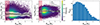 |
Fig. 9. Properties of the PAH clouds vs Rgal for all the clouds in the 66 galaxies: Σmol of the cloud (left), Req (middle), and the total number of galaxies contributing to a specific bin (right). The running galaxy median (filled black circles) is plotted for a bin width of 0.2 Re. The gray-shaded region represents the interquartile range of the medians per galaxy. The error bars on the median are the standard errors (1.253σ/ |

In the PHANGS–ALMA sample (e.g., Sun et al. 2020b; Leroy et al. 2025), cloud-scale Σmol shows little variation with Rgal beyond the central regions, in agreement with our results. Also, at fixed Rgal/Re, PAH clouds located in spiral arms exhibit Σmol values approximately 1.5–2.5 times higher than those in interarm regions (see Fig. D.2), consistent with the spiral arm–interarm contrast observed in PHANGS–ALMA.
We find that the galaxy-by-galaxy Σmol in Figs. D.1 and D.3 show considerable variation with Rgal, with flat, declining, and ambiguous profiles observed across different galaxies. The Σmol behavior in some CO-based cloud analysis (e.g., Rebolledo et al. 2015; Faesi et al. 2018) show no clear trend with Rgal, highlighting that, in some galaxies, the galactic environment might play a bigger role in determining the GMC properties than a radial-based approach. An example of this in our sample would be NGC 0628, NGC 1365, NGC 2090, and NGC 2997 (see Fig. D.1), where the spiral arm-interarm contrast exists, but there is a flat Σmol trend with Rgal. However, in other galaxies, such as NGC 1385, NGC 1546, NGC 1559, and NGC 3059, that lack spiral arm features, we see a ∼0.5–1 dex decrease of Σmol toward the outer regions of the galaxies. Together, these examples highlight that radial trends in cloud Σmol are not universal, but instead vary strongly with different galaxies.
5.5. Extreme clouds
In this section, we focus on clouds at the extremes of both Σmol and Mmol within our sample. An overabundance of high Σmol and high Mmol clouds in specific large-scale galactic environments suggests that localized physical processes in these regions preferentially drive the formation of distinct, dense, and massive cloud populations, potentially enhancing star formation activity. Conversely, the prevalence of low Σmol and low-mass clouds in certain environments may indicate the presence of mechanisms that inhibit efficient gas compression and cloud growth, such as strong shear, elevated turbulence, or low external pressure. These processes act to suppress the formation of gravitationally bound and massive structures, ultimately limiting star formation efficiency.
We define low-mass Σmol clouds as clouds with Σmol ≤ 10 M⊙ pc−2, representing ∼32% of our sample size, and extremely low Σmol clouds are the 1000 least dense clouds. The highest Σmol clouds are clouds with Σmol ≥ 100 M⊙ pc−2, representing ∼5% of our sample size, and the extremely highest Σmol clouds are the 1000 highest dense clouds.
We rely on fractional differences between the full sample and low- or high-density clouds per galactic environment to assess where those clouds prevail more. The fractional difference is then defined as
 (15)
(15)
where  is the number of extreme clouds in a specific environment from the extreme subsample (Nsub), and
  is the number of clouds in a specific environment in the full sample (Nsample).
A positive Δf value would indicate, probabilistically, higher prevalence in a specific environment. The values of Δflow, Δfhigh,  , and
, and  are provided in Table 5. Here, Δflow, Δfhigh are the fractional differences between the full sample and the low or high Σmol regimes, respectively. The notation “e” is for the extreme samples.
Pearson χ2 and fractional difference statistical tests for the extreme cloud subsamples.
The Δf values presented in Table 5 indicate that the low Σmol clouds are most frequent in bar and interarm regions and are the least frequent in spiral arm regions. Also, the highest Σmol clouds are most and least prevalent in spiral arm and interarm regions, respectively. We note that extremely low Σmol in bars could be due to the under-approximation of the CO emission in bar ends and the αCO prescription used here, and due to the existence of low Σmol clouds in bar lanes. Upon using the other αCO prescriptions, we notice that our results are consistent in all the environments except the bar region, where interarm clouds take over as the lowest density structures.
Sun et al. (2022) further demonstrate that in the PHANGS-ALMA sample, CO cloud properties correlate strongly with environmental conditions, particularly ΣSFR and Σmol. Together with our results, these studies support the picture where spiral arms are key sites for the formation of dense, high Σmol and high-mass clouds, while the interarm regions are mainly populated by diffuse and lower-mass clouds. Again, we emphasize that central regions were excluded from our main analysis due to the removal of overlapping structures. However, when we include the central clouds, they emerge as the primary hosts of the extremely highest density clouds, consistent with both Galactic and extragalactic observations (e.g., Longmore et al. 2012; Mills 2017; Sun et al. 2018, 2020b), followed by the spiral arms.
Many galactic factors play a role in shaping the clouds across the mass distribution and spectra. The high-mass clouds are intrinsically rarer than lower-mass clouds (∼4% of our sample size). Kobayashi et al. (2017) (see also Tasker & Tan 2009; Kobayashi et al. 2018) show that in simulated clouds, cloud-cloud collisions mostly affect the tail of the cloud mass spectra. Those collisions lead to the formation of more massive GMCs (Mmol ≳ 106 M⊙). Kruijssen (2014) suggested that the maximum GMC mass may correspond to the maximum mass that could collapse against centrifugal forces (i.e., Toomre mass; Toomre 1964). Models that predict the maximum GMC mass (e.g., Reina-Campos & Kruijssen 2017) explain that those masses change from shear-limited to feedback-limited as galaxies become less gas-rich and evolve toward low shear. The s parameter of the lognormal has a strong positive correlation with the high-mass cloud fraction, implying that more massive clouds exist at higher s values. At lower masses, cloud self-growth by accumulating surrounding HI gas and destruction by massive star radiative feedback (e.g., due to photo-ionization, photo-dissociation) shape the cloud mass spectra. Upon binning the Mmol distribution, we examine the correlation between the total mass in each bin and various global galaxy properties across our sample (see Fig. D.6). We find that only clouds with Mmol between 104 and 106 M⊙, which make up 90% of the sample, show a significant positive correlation with both the HI mass and the star formation rate (SFR) of their host galaxies (see Fig. D.6). In contrast, clouds with Mmol below 104 M⊙ show no apparent correlation with global SFR or HI mass. This suggests that massive star formation is not prominent in these lower-mass clouds.
6. Summary and conclusion
In this paper, we utilized SCIMES (C15), an unsupervised clustering algorithm, to identify cloud structures in 66 nearby PHANGS-JWST galaxies (Lee et al. 2023; Williams et al. 2024). Using stellar continuum-corrected IF770WPAH maps, we identified 108 466 and 146 040 clouds in the common-resolution and native resolution samples, respectively. This represents the largest extragalactic cloud catalog to date. We used the common resolution sample for our analysis. We also flagged and excluded from our analysis clouds dominated by IF770WPAH < 1 MJy sr−1, those located at the edges of the maps, and those overlapping in velocity space when cross-matched with CO-identified clouds using CPROPS (Hughes et al., in prep.). After these exclusions, the final sample consists of 77 884 clouds. Those strict measures were taken to avoid any biases. This results in a significant loss of high Σmol clouds, mostly toward galactic centers, which we therefore excluded from our analysis.
Upon comparing the IF770WPAH identified clouds to CO-identified clouds, we notice an agreement in the Σmol between both methods in the different environments. We refer to the identified clouds as GMCs; however, regions with Σmol ≤ 10 M⊙ pc−2 may correspond to either diffuse atomic gas or faint molecular clouds that remain undetectable in CO observations. Upon examining these regions, we find that such clouds are predominantly located in the interarm and disk regions, reinforcing our previous assertion.
When investigating the Σmol CDFs and distributions across different environments, we find that the spiral arms contain the highest number density of clouds (including high Σmol clouds), and the interarm clouds show a sharper decline in Σmol values after 10 M⊙ pc−2. This observation is further backed by our fractional difference test, which confirms that spiral arms preferentially host the highest Σmol clouds. Our findings generally align with hydrodynamical simulations (e.g., Duarte-Cabral & Dobbs 2016) where the highest Σmol GMC complexes are in the spiral arms. This also agrees with the idea that the gravitational potential of spiral arms aids in the formation of high Σmol clouds, which subsequently fragment into less dense structures as they drift into interarm regions (e.g., Dobbs et al. 2006; Koda et al. 2009).
We also fit a lognormal to the mass spectra with a completeness limit extending down to 2 × 10³ M⊙, well below previously obtained depths with CO observations, and find that it represents a good fit. Spiral arm clouds tend to have more massive clouds than the other environments according to the s and σ of the lognormal distribution fits. Positive correlations exist between both the sgal and σgal of clouds, sSFR, and the median Σmol of the galaxies, reflecting that galaxies that host more massive clouds have more star formation with respect to their stellar mass.
The cloud properties show minimal variation as a function of Rgal. The Req of the clouds is consistent toward the outskirts of the galaxies. Meanwhile, the cloud Σmol values decrease by a factor of ∼1.5 − 2 toward the outer parts of the galaxies. Also, at a fixed Rgal/Re, spiral arms have Σmol values approximately 1.5–2.5 times higher than those in interarm regions. It is worth noting that Σmol trend varies largely between different galaxies, with flat, decreasing, and even no trend as a function of Rgal. Factors such as large-scale processes, galaxy types, and morphologies might influence the observed trends.
The cloud mass spectra, radial profiles, and properties vary from galaxy to galaxy depending on their physical conditions and local environments. In contrast, combining all clouds across galaxies averages out this local information, emphasizing only global environmental differences between galaxies.
We list a few key points to summarize our findings:
-
A total of 108 466 PAH clouds were identified across 66 galaxies using SCIMES. Of these, 77 844 clouds met or selection criteria and were included in the analysis, while others were flagged in the catalog (e.g., for velocity overlap, edge effects, low molecular gas content) and excluded from the analysis. This led to a bias toward lower Σmol clouds, evidenced by a reduced PAH cloud flux recovery (a median of 26% in the flagged sample vs 40% in the full sample).
-
The PAH clouds reveal fainter, smaller structures, especially in the interarm and bar regions, compared to CO-based ALMA clouds (∼2 dex better completeness limit). Those clouds may correspond to either faint molecular clouds or diffuse atomic gas clouds, or be sensitivity-limited in CO observations.
-
Both PAH and CO identified clouds show consistent Σmol, R distributions across most environments. However, toward central regions, PAH cloud Σmol, R is 0.3 dex lower. This could be due to the PAH-to-CO fit, αCO prescription, and overlapping clouds in velocity pose a challenge in our analysis, making it challenging to derive any conclusions there.
-
The cloud Σmol varies with galactic environment, with spiral arms hosting the highest Σmol and Mmol clouds, interarms and bars the least, and disks showing intermediate properties of spiral arms and interarms. This supports the view that spiral arm potentials favor the formation of massive, dense clouds consistent with both observations and simulations.
-
The mass spectra are better described by a lognormal distribution than a single power law, especially when considering a large cloud sample, with lognormal μ and σ indicating that spiral arms host more massive clouds and a shallower mass spectrum compared to other environments.
-
Variations in the cloud mass spectrum are more strongly influenced by differences between galaxies than by intra-galactic environments. This indicates that global galaxy properties such as gas content, star formation activity, and dynamics are the primary factors shaping the distribution of cloud masses.
-
The cloud Σmol values shows a decline of a factor of ∼1.5 − 2 toward the outskirts of the galaxies (2–3 Re), and at fixed Rgal/Re, PAH clouds located in spiral arms exhibit Σmol values approximately 1.5–2.5 times higher than those in interarm regions.
-
The clouds with Mmol > 104 M⊙ show a positive correlation with SFR, indicating that these clouds are key contributors to star formation. Meanwhile, clouds with Mmol < 104 M⊙ do not show a correlation, indicating limited involvement in large-scale star-forming activity, or that their star formation is below detection limits.
-
We publish our PAH cloud catalog at a homogenized resolution of 30 pc and native resolution. The catalog includes measurements of Mmol, Req, Σmol, and other parameters presented in Table C.1.
We emphasize the importance of handling PP intensity images with care when identifying structure. We showed how including overlapping clouds could bias the results, and excluding them could push the analysis toward lower Σmol and Mmol clouds. Our findings provide valuable insights and calibrations for molecular cloud simulations, especially the mass spectra depicted here. Future work could include calibrating the CO to PAH relationship while subtracting the emission from small dust grains. Those grains could play a significant role, especially toward the central regions of the galaxies.
Data availability
The full figure of Appendix D (Fig. D.1) is available on Zenodo at https://zenodo.org/records/15428261. Table C.1 is available at the CDS via https://cdsarc.cds.unistra.fr/viz-bin/cat/J/A+A/706/A40
Acknowledgments
This work has been carried out as part of the PHANGS collaboration. This work is based on observations made with the NASA/ESA/CSA JWST. The data were obtained from the Mikulski Archive for Space Telescopes at the Space Telescope Science Institute, which is operated by the Association of Universities for Research in Astronomy, Inc., under NASA contract NAS 5-03127 for JWST. These observations are associated with programs 2107 and 3707. ZB, DC, and FB gratefully acknowledge the Collaborative Research Center 1601 (SFB 1601 sub-project B3) funded by the Deutsche Forschungsgemeinschaft (DFG, German Research Foundation) – 500700252. DC acknowledges support by the Deutsche Forschungsgemeinschaft, DFG project number SFB956-A3. A.K.L., S.S., and R.C. gratefully acknowledge support from NSF AST AWD 2205628, JWST-GO-02107.009-A, and JWST-GO-03707.001-A. A.K.L. also gratefully acknowledges support by a Humboldt Research Award. H.F.V. acknowledges support from the Swedish National Space Agency (SNSA) through the grant 2023-00260, and support from RS 31004975. A.D.C. acknowledges the support from the Royal Society University Research Fellowship URF/R1/191609. E.R. acknowledges support from the Canadian Space Agency, funding reference 23JWGO2A07. R.S.K. and S.C.O.G. acknowledge financial support from ERC via Synergy Grant “ECOGAL” (project ID 855130), from the German Excellence Strategy via the “STRUCTURES” Cluster of Excellence (EXC 2181–390900948), and from the German Ministry for Economic Affairs and Climate Action in project “MAINN” (funding ID 50OO2206). R.S.K. also thanks the 2024/25 Class of Radcliffe Fellows for their company and for highly stimulating discussions. K.S. acknowledges funding support from grants JWST-GO-02107.006-A and JWST-GO-03707.005-A. Finally, we thank the anonymous referee for the helpful suggestions, which improved the quality of this paper. This research made use of Astropy (http://www.astropy.org) a community-developed core Python package for Astronomy (Astropy Collaboration 2013, 2018); matplotlib (Hunter 2007); numpy and scipy (Virtanen et al. 2020).
References
- Asplund, M., Grevesse, N., Sauval, A. J., & Scott, P. 2009, ARA&A, 47, 481 [NASA ADS] [CrossRef] [Google Scholar]
- Astropy Collaboration (Robitaille, T. P., et al.) 2013, A&A, 558, A33 [NASA ADS] [CrossRef] [EDP Sciences] [Google Scholar]
- Astropy Collaboration (Price-Whelan, A. M., et al.) 2018, AJ, 156, 123 [Google Scholar]
- Baron, D., Sandstrom, K. M., Rosolowsky, E., et al. 2024, ApJ, 968, 24 [NASA ADS] [CrossRef] [Google Scholar]
- Belfiore, F., Leroy, A. K., Williams, T. G., et al. 2023, A&A, 678, A129 [NASA ADS] [CrossRef] [EDP Sciences] [Google Scholar]
- Bigiel, F., Leroy, A., Walter, F., et al. 2008, AJ, 136, 2846 [NASA ADS] [CrossRef] [Google Scholar]
- Blitz, L., Fukui, Y., Kawamura, A., et al. 2007, in Protostars and Planets V, eds. B. Reipurth, D. Jewitt, & K. Keil, 81 [Google Scholar]
- Bohlin, R. C., Savage, B. D., & Drake, J. F. 1978, ApJ, 224, 132 [Google Scholar]
- Bolatto, A. D., Leroy, A. K., Rosolowsky, E., Walter, F., & Blitz, L. 2008, ApJ, 686, 948 [NASA ADS] [CrossRef] [Google Scholar]
- Bolatto, A. D., Wolfire, M., & Leroy, A. K. 2013, ARA&A, 51, 207 [CrossRef] [Google Scholar]
- Calzetti, D., Kennicutt, R. C., Engelbracht, C. W., et al. 2007, ApJ, 666, 870 [Google Scholar]
- Casoli, F., & Combes, F. 1982, A&A, 110, 287 [NASA ADS] [Google Scholar]
- Chevance, M., Kruijssen, J. M. D., Vazquez-Semadeni, E., et al. 2020, Space Sci. Rev., 216, 50 [NASA ADS] [CrossRef] [Google Scholar]
- Chown, R., Li, C., Parker, L., et al. 2020, MNRAS, 500, 1261 [NASA ADS] [CrossRef] [Google Scholar]
- Chown, R., Leroy, A. K., Sandstrom, K., et al. 2025, ApJ, 983, 64 [Google Scholar]
- Colman, T., Brucy, N., Girichidis, P., et al. 2024, A&A, 686, A155 [NASA ADS] [CrossRef] [EDP Sciences] [Google Scholar]
- Colombo, D., Hughes, A., Schinnerer, E., et al. 2014, ApJ, 784, 3 [NASA ADS] [CrossRef] [Google Scholar]
- Colombo, D., Rosolowsky, E., Ginsburg, A., Duarte-Cabral, A., & Hughes, A. 2015, MNRAS, 454, 2067 [NASA ADS] [CrossRef] [Google Scholar]
- Colombo, D., Rosolowsky, E., Duarte-Cabral, A., et al. 2019, MNRAS, 483, 4291 [NASA ADS] [CrossRef] [Google Scholar]
- Cortzen, I., Garrett, J., Magdis, G., et al. 2018, MNRAS, 482, 1618 [Google Scholar]
- Dale, D. A., Graham, G. B., Barnes, A. T., et al. 2025, AJ, 169, 133 [Google Scholar]
- Dame, T. M., Hartmann, D., & Thaddeus, P. 2001, ApJ, 547, 792 [Google Scholar]
- Demachi, F., Fukui, Y., Yamada, R. I., et al. 2024, PASJ, 76, 1059 [Google Scholar]
- den Brok, J. S., Cantalupo, S., Mackenzie, R., et al. 2020, MNRAS, 495, 1874 [Google Scholar]
- Dobbs, C. L. 2008, MNRAS, 391, 844 [NASA ADS] [CrossRef] [Google Scholar]
- Dobbs, C. L. 2015, MNRAS, 447, 3390 [CrossRef] [Google Scholar]
- Dobbs, C. L., & Pringle, J. E. 2013, MNRAS, 432, 653 [NASA ADS] [CrossRef] [Google Scholar]
- Dobbs, C. L., Bonnell, I. A., & Pringle, J. E. 2006, MNRAS, 371, 1663 [Google Scholar]
- Dobbs, C. L., Burkert, A., & Pringle, J. E. 2011, MNRAS, 417, 1318 [NASA ADS] [CrossRef] [Google Scholar]
- Dobbs, C. L., Pringle, J. E., & Duarte-Cabral, A. 2014, MNRAS, 446, 3608 [Google Scholar]
- Draine, B. T., & Li, A. 2007, ApJ, 657, 810 [CrossRef] [Google Scholar]
- Duarte-Cabral, A., & Dobbs, C. L. 2016, MNRAS, 458, 3667 [NASA ADS] [CrossRef] [Google Scholar]
- Duarte-Cabral, A., & Dobbs, C. L. 2017, MNRAS, 470, 4261 [NASA ADS] [CrossRef] [Google Scholar]
- Duarte-Cabral, A., Colombo, D., Urquhart, J. S., et al. 2020, MNRAS, 500, 3027 [NASA ADS] [CrossRef] [Google Scholar]
- Eden, D., Moore, T., Plume, R., & Morgan, L. 2012, MNRAS, 422, 3178 [NASA ADS] [CrossRef] [Google Scholar]
- Egorov, O. V., Leroy, A. K., Sandstrom, K., et al. 2025, A&A, 703, A103 [NASA ADS] [CrossRef] [EDP Sciences] [Google Scholar]
- Elmegreen, B. 2011, EAS Publ. Ser., 51, 19 [Google Scholar]
- Faesi, C. M., Lada, C. J., & Forbrich, J. 2018, ApJ, 857, 19 [NASA ADS] [CrossRef] [Google Scholar]
- Faustino Vieira, H., Duarte-Cabral, A., Davis, T. A., et al. 2023, MNRAS, 524, 161 [Google Scholar]
- Faustino Vieira, H., Duarte-Cabral, A., Davis, T. A., et al. 2024, MNRAS, 527, 3639 [Google Scholar]
- Faustino Vieira, H., Duarte-Cabral, A., Smith, M. W. L., et al. 2025, MNRAS, 538, 2744 [Google Scholar]
- Field, G. B., & Saslaw, W. C. 1965, ApJ, 142, 568 [NASA ADS] [Google Scholar]
- Fujimoto, Y., Tasker, E. J., Wakayama, M., & Habe, A. 2014, MNRAS, 439, 936 [NASA ADS] [CrossRef] [Google Scholar]
- Fukui, Y., & Kawamura, A. 2010, ARA&A, 48, 547 [NASA ADS] [CrossRef] [Google Scholar]
- Fukui, Y., Mizuno, N., Yamaguchi, R., Mizuno, A., & Onishi, T. 2001, PASJ, 53, L41 [Google Scholar]
- Gao, Y., Xiao, T., Li, C., et al. 2019, ApJ, 887, 172 [Google Scholar]
- Gao, Y., Tan, Q.-H., Gao, Y., et al. 2022, ApJ, 940, 133 [NASA ADS] [CrossRef] [Google Scholar]
- García-Bernete, I., Rigopoulou, D., Alonso-Herrero, A., et al. 2022, A&A, 666, L5 [NASA ADS] [CrossRef] [EDP Sciences] [Google Scholar]
- García-Bernete, I., Rigopoulou, D., Donnan, F. R., et al. 2024, A&A, 691, A162 [NASA ADS] [CrossRef] [EDP Sciences] [Google Scholar]
- Glover, S., & Low, M.-M. M. 2011, MNRAS, 412, 337 [NASA ADS] [CrossRef] [Google Scholar]
- Glover, S. C. O., & Smith, R. J. 2016, MNRAS, 462, 3011 [NASA ADS] [CrossRef] [Google Scholar]
- Grand, R. J. J., Gómez, F. A., Marinacci, F., et al. 2017, MNRAS, 467, 179 [NASA ADS] [Google Scholar]
- Heyer, M. H., Carpenter, J. M., & Snell, R. L. 2001, ApJ, 551, 852 [NASA ADS] [CrossRef] [Google Scholar]
- Heyer, M., Krawczyk, C., Duval, J., & Jackson, J. M. 2009, ApJ, 699, 1092 [Google Scholar]
- Hirota, A., Kuno, N., Sato, N., et al. 2011, ApJ, 737, 40 [NASA ADS] [CrossRef] [Google Scholar]
- Hopkins, P. F., Wetzel, A., Kereš, D., et al. 2018, MNRAS, 480, 800 [NASA ADS] [CrossRef] [Google Scholar]
- Houck, J. R., Roellig, T. L., van Cleve, J., et al. 2004, ApJS, 154, 18 [NASA ADS] [CrossRef] [Google Scholar]
- Houlahan, P., & Scalo, J. 1992, ApJ, 393, 172 [CrossRef] [Google Scholar]
- Hu, C.-Y., Schruba, A., Sternberg, A., & van Dishoeck, E. F. 2022, ApJ, 931, 28 [NASA ADS] [CrossRef] [Google Scholar]
- Hughes, A., Meidt, S. E., Colombo, D., et al. 2013, ApJ, 779, 46 [NASA ADS] [CrossRef] [Google Scholar]
- Hunter, J. D. 2007, Comput. Sci. Eng., 9, 90 [NASA ADS] [CrossRef] [Google Scholar]
- Jameson, K. E., Bolatto, A. D., Leroy, A. K., et al. 2016, ApJ, 825, 12 [NASA ADS] [CrossRef] [Google Scholar]
- Jeffreson, S. M. R., & Kruijssen, J. M. D. 2018, MNRAS, 476, 3688 [Google Scholar]
- Kobayashi, M. I. N., Inutsuka, S.-I., Kobayashi, H., & Hasegawa, K. 2017, ApJ, 836, 175 [NASA ADS] [CrossRef] [Google Scholar]
- Kobayashi, M. I. N., Kobayashi, H., Inutsuka, S.-I., & Fukui, Y. 2018, PASJ, 70, S59 [NASA ADS] [CrossRef] [Google Scholar]
- Koda, J., Scoville, N., Sawada, T., et al. 2009, ApJ, 700, L132 [NASA ADS] [CrossRef] [Google Scholar]
- Kruijssen, J. M. D. 2014, Class. Quant. Grav., 31, 244006 [NASA ADS] [CrossRef] [Google Scholar]
- Lee, J. C., Sandstrom, K. M., Leroy, A. K., et al. 2023, ApJ, 944, L17 [NASA ADS] [CrossRef] [Google Scholar]
- Leroy, A. K., Bolatto, A., Gordon, K., et al. 2011, ApJ, 737, 12 [Google Scholar]
- Leroy, A. K., Walter, F., Sandstrom, K., et al. 2013, AJ, 146, 19 [Google Scholar]
- Leroy, A. K., Hughes, A., Schruba, A., et al. 2016, ApJ, 831, 16 [Google Scholar]
- Leroy, A. K., Schinnerer, E., Hughes, A., et al. 2021, ApJS, 257, 43 [NASA ADS] [CrossRef] [Google Scholar]
- Leroy, A. K., Rosolowsky, E., Usero, A., et al. 2022, ApJ, 927, 149 [NASA ADS] [CrossRef] [Google Scholar]
- Leroy, A. K., Bolatto, A. D., Sandstrom, K., et al. 2023a, ApJ, 944, L10 [NASA ADS] [CrossRef] [Google Scholar]
- Leroy, A. K., Sandstrom, K., Rosolowsky, E., et al. 2023b, ApJ, 944, L9 [NASA ADS] [CrossRef] [Google Scholar]
- Leroy, A. K., Sun, J., Meidt, S., et al. 2025, ApJ, 985, 14 [Google Scholar]
- Lin, C. C., & Shu, F. H. 1964, ApJ, 140, 646 [Google Scholar]
- Longmore, S. N., Bally, J., Testi, L., et al. 2012, MNRAS, 429, 987 [Google Scholar]
- Mazumdar, P., Wyrowski, F., Urquhart, J. S., et al. 2021, A&A, 656, A101 [NASA ADS] [CrossRef] [EDP Sciences] [Google Scholar]
- Meidt, S. E., Schinnerer, E., García-Burillo, S., et al. 2013, ApJ, 779, 45 [NASA ADS] [CrossRef] [Google Scholar]
- Meidt, S. E., Leroy, A. K., Rosolowsky, E., et al. 2018, ApJ, 854, 100 [NASA ADS] [CrossRef] [Google Scholar]
- Meidt, S. E., Leroy, A. K., Querejeta, M., et al. 2021, ApJ, 913, 113 [NASA ADS] [CrossRef] [Google Scholar]
- Meidt, S. E., Rosolowsky, E., Sun, J., et al. 2023, ApJ, 944, L18 [CrossRef] [Google Scholar]
- Meyer, J. D., Koda, J., Momose, R., et al. 2013, ApJ, 772, 107 [NASA ADS] [CrossRef] [Google Scholar]
- Mills, E. A. C. 2017, arXiv e-prints [arXiv:1705.05332] [Google Scholar]
- Mok, A., Chandar, R., & Fall, S. M. 2020, ApJ, 893, 135 [NASA ADS] [CrossRef] [Google Scholar]
- Nimori, M., Habe, A., Sorai, K., et al. 2012, MNRAS, 429, 2175 [Google Scholar]
- Pathak, D., Leroy, A. K., Thompson, T. A., et al. 2024, AJ, 167, 39 [NASA ADS] [CrossRef] [Google Scholar]
- Peeters, E., Spoon, H. W. W., & Tielens, A. G. G. M. 2004, ApJ, 613, 986 [NASA ADS] [CrossRef] [Google Scholar]
- Pettini, M., & Pagel, B. E. J. 2004, MNRAS, 348, L59 [NASA ADS] [CrossRef] [Google Scholar]
- Pettitt, A. R., Dobbs, C. L., Baba, J., et al. 2020, MNRAS, 498, 1159 [Google Scholar]
- Querejeta, M., Schinnerer, E., Meidt, S., et al. 2021, A&A, 656, A133 [NASA ADS] [CrossRef] [EDP Sciences] [Google Scholar]
- Querejeta, M., Leroy, A. K., Meidt, S. E., et al. 2024, A&A, 687, A293 [NASA ADS] [CrossRef] [EDP Sciences] [Google Scholar]
- Ragan, S. E., Henning, T., Tackenberg, J., et al. 2014, A&A, 568, A73 [NASA ADS] [CrossRef] [EDP Sciences] [Google Scholar]
- Rebolledo, D., Wong, T., Leroy, A., Koda, J., & Meyer, J. D. 2012, ApJ, 757, 155 [CrossRef] [Google Scholar]
- Rebolledo, D., Wong, T., Xue, R., et al. 2015, ApJ, 808, 99 [NASA ADS] [CrossRef] [Google Scholar]
- Regan, M. W., Thornley, M. D., Bendo, G. J., et al. 2004, ApJS, 154, 204 [Google Scholar]
- Regan, M. W., Thornley, M. D., Vogel, S. N., et al. 2006, ApJ, 652, 1112 [NASA ADS] [CrossRef] [Google Scholar]
- Reina-Campos, M., & Kruijssen, J. M. D. 2017, MNRAS, 469, 1282 [CrossRef] [Google Scholar]
- Roberts, W. W., Jr., Huntley, J. M., & van Albada, G. D. 1979, ApJ, 233, 67 [NASA ADS] [CrossRef] [Google Scholar]
- Roman-Duval, J., Jackson, J. M., Heyer, M., Rathborne, J., & Simon, R. 2010, ApJ, 723, 492 [NASA ADS] [CrossRef] [Google Scholar]
- Rosolowsky, E. 2005, PASP, 117, 1403 [NASA ADS] [CrossRef] [Google Scholar]
- Rosolowsky, E., & Blitz, L. 2005, ApJ, 623, 826 [NASA ADS] [CrossRef] [Google Scholar]
- Rosolowsky, E., & Leroy, A. 2006, PASP, 118, 590 [NASA ADS] [CrossRef] [Google Scholar]
- Rosolowsky, E. W., Pineda, J. E., Kauffmann, J., & Goodman, A. A. 2008, ApJ, 679, 1338 [Google Scholar]
- Rosolowsky, E., Hughes, A., Leroy, A. K., et al. 2021, MNRAS, 502, 1218 [NASA ADS] [CrossRef] [Google Scholar]
- Saintonge, A., & Catinella, B. 2022, ARA&A, 60, 319 [NASA ADS] [CrossRef] [Google Scholar]
- Sánchez, S. F., Rosales-Ortega, F. F., Iglesias-Páramo, J., et al. 2014, A&A, 563, A49 [CrossRef] [EDP Sciences] [Google Scholar]
- Sánchez, S. F., Barrera-Ballesteros, J. K., López-Cobá, C., et al. 2019, MNRAS, 484, 3042 [CrossRef] [Google Scholar]
- Sanders, D. B., & Mirabel, I. F. 1985, ApJ, 298, L31 [Google Scholar]
- Sandstrom, K. M., Chastenet, J., Sutter, J., et al. 2023, ApJ, 944, L7 [NASA ADS] [CrossRef] [Google Scholar]
- Sandstrom, K. M., Koch, E. W., Leroy, A. K., et al. 2023, ApJ, 944, L8 [NASA ADS] [CrossRef] [Google Scholar]
- Savage, B. D., & Mathis, J. S. 1979, ARA&A, 17, 73 [NASA ADS] [CrossRef] [Google Scholar]
- Savage, B. D., Bohlin, R. C., Drake, J. F., & Budich, W. 1977, ApJ, 216, 291 [NASA ADS] [CrossRef] [Google Scholar]
- Schinnerer, E., & Leroy, A. 2024, ARA&A, 62, 369 [NASA ADS] [CrossRef] [Google Scholar]
- Schruba, A., Leroy, A. K., Walter, F., et al. 2011, AJ, 142, 37 [NASA ADS] [CrossRef] [Google Scholar]
- Scoville, N. Z., & Hersh, K. 1979, ApJ, 229, 578 [NASA ADS] [CrossRef] [Google Scholar]
- Sheth, K., Regan, M., Hinz, J. L., et al. 2010, PASP, 122, 1397 [Google Scholar]
- Shivaei, I., & Boogaard, L. A. 2024, A&A, 691, L2 [NASA ADS] [CrossRef] [EDP Sciences] [Google Scholar]
- Smith, J. D. T., Draine, B. T., Dale, D. A., et al. 2007, ApJ, 656, 770 [Google Scholar]
- Smith, R. J., Glover, S. C. O., Clark, P. C., Klessen, R. S., & Springel, V. 2014, MNRAS, 441, 1628 [NASA ADS] [CrossRef] [Google Scholar]
- Smith, R. J., Treß, R. G., Sormani, M. C., et al. 2020, MNRAS, 492, 1594 [NASA ADS] [CrossRef] [Google Scholar]
- Solomon, P. M., Rivolo, A. R., Barrett, J., & Yahil, A. 1987, ApJ, 319, 730 [Google Scholar]
- Sormani, M. C., & Barnes, A. T. 2019, MNRAS, 484, 1213 [NASA ADS] [CrossRef] [Google Scholar]
- Spoon, H. W. W., Marshall, J. A., Houck, J. R., et al. 2006, ApJ, 654, L49 [Google Scholar]
- Stutzki, J., & Guesten, R. 1990, ApJ, 356, 513 [Google Scholar]
- Sun, J., Leroy, A. K., Schruba, A., et al. 2018, ApJ, 860, 172 [NASA ADS] [CrossRef] [Google Scholar]
- Sun, J., Leroy, A. K., Ostriker, E. C., et al. 2020a, ApJ, 892, 148 [NASA ADS] [CrossRef] [Google Scholar]
- Sun, J., Leroy, A. K., Schinnerer, E., et al. 2020b, ApJ, 901, L8 [NASA ADS] [CrossRef] [Google Scholar]
- Sun, J., Leroy, A. K., Rosolowsky, E., et al. 2022, AJ, 164, 43 [NASA ADS] [CrossRef] [Google Scholar]
- Sun, J., Leroy, A. K., Ostriker, E. C., et al. 2023, ApJ, 945, L19 [NASA ADS] [CrossRef] [Google Scholar]
- Sutter, J., Sandstrom, K., Chastenet, J., et al. 2024, ApJ, 971, 178 [NASA ADS] [CrossRef] [Google Scholar]
- Taff, L. G., & Savedoff, M. P. 1972, MNRAS, 160, 89 [Google Scholar]
- Tasker, E. J., & Tan, J. C. 2009, ApJ, 700, 358 [NASA ADS] [CrossRef] [Google Scholar]
- Teng, Y.-H., Chiang, I.-D., Sandstrom, K. M., et al. 2024, ApJ, 961, 42 [NASA ADS] [CrossRef] [Google Scholar]
- Thilker, D. A., Lee, J. C., Deger, S., et al. 2023, ApJ, 944, L13 [NASA ADS] [CrossRef] [Google Scholar]
- Tielens, A. G. G. M. 2008, ARA&A, 46, 289 [NASA ADS] [CrossRef] [Google Scholar]
- Toomre, A. 1964, ApJ, 139, 1217 [Google Scholar]
- Treß, R. G., Sormani, M. C., Smith, R. J., et al. 2021, MNRAS, 505, 5438 [NASA ADS] [CrossRef] [Google Scholar]
- Usero, A., Leroy, A. K., Walter, F., et al. 2015, AJ, 150, 115 [Google Scholar]
- van Dishoeck, E. F., & Black, J. H. 1988, ApJ, 334, 771 [Google Scholar]
- Véron-Cetty, M. P., & Véron, P. 2010, A&A, 518, A10 [Google Scholar]
- Verwilghen, P., Emsellem, E., Renaud, F., et al. 2025, A&A, 700, A3 [NASA ADS] [CrossRef] [EDP Sciences] [Google Scholar]
- Virtanen, P., Gommers, R., Oliphant, T. E., et al. 2020, Nat. Methods, 17, 261 [Google Scholar]
- Whitcomb, C. M., Sandstrom, K., Leroy, A., & Smith, J.-D. T. 2023, ApJ, 948, 88 [CrossRef] [Google Scholar]
- Whitcomb, C. M., Sandstrom, K., & Smith, J.-D. T. 2023, Res. Notes AAS, 7, 38 [Google Scholar]
- Williams, J. P., de Geus, E. J., & Blitz, L. 1994, ApJ, 428, 693 [Google Scholar]
- Williams, T. G., Lee, J. C., Larson, K. L., et al. 2024, ApJS, 273, 13 [NASA ADS] [CrossRef] [Google Scholar]
- Wolfire, M. G., Hollenbach, D., & McKee, C. F. 2010, ApJ, 716, 1191 [Google Scholar]
- Wright, E. L., Eisenhardt, P. R. M., Mainzer, A. K., et al. 2010, AJ, 140, 1868 [Google Scholar]
- Yu, S.-Y., Kalinova, V., Colombo, D., et al. 2022, A&A, 666, A175 [NASA ADS] [CrossRef] [EDP Sciences] [Google Scholar]
The upper limit is the difference between the 84th and 50th percentiles, and the lower limit is between the 50th and 16th percentiles of the fraction of flux within the clouds in the 66 galaxies.
Appendix A: SCIMES version update
In this study, we implemented a modification to SCIMES to enhance computational efficiency. The primary modification involved implementing parallel processing using the Parallel9 function from the joblib10 library in Python. This optimization was applied to the spectral embedding step, where dimensionality reduction is performed.
To make use of the parallel processing feature, an additional parameter was added (n_jobs = −1). The n_jobs parameter controls the number of concurrent tasks executed in parallel. When set to a positive integer, it specifies the exact number of worker processes or threads used for computation. If n_jobs = −1, the system utilizes all available CPU cores, while n_jobs = −2 reserves one core for other tasks. If n_jobs = 1, the code runs sequentially, similar to a standard Python loop. This improvement significantly reduces processing time, particularly when handling large molecular cloud datasets.
This modified version of SCIMES was used throughout this analysis and is available on the following GitHub11 page.
Appendix B: Tables of properties
The global and cloud properties of 66 galaxies in the PHANGS-JWST sample.
Appendix C: Catalog information
PAH cloud catalog columns and their descriptions.
We publish two catalogs, one at the native resolution and sensitivity of each galaxy and another at the homogenized resolution of 30 pc and a common sensitivity of 0.19 MJy sr−1. The Mmol estimates using the different prescriptions are calculated for all the clouds in the different galaxies, except for two galaxies (NGC 4424 and NGC 4694) using the Teng et al. (2024) prescription.
The native resolution sample comprises 146,040 PAH clouds, and 108,019 clouds after flagging using fall. The min_npix is set to be 3 × Ωbeam/Ωpix, instead of 1 × Ωbeam/Ωpix for this sample. This measure was taken to decrease the segmentation error on the smallest structures. Additionally, the scaling parameter implementation is similar to the homogenized sample.
Appendix D: Additional plots
D.1. Galaxy-by-galaxy property plots
|
Fig. D.1. Summary of galaxy-by-galaxy properties. The plots are available at https://zenodo.org/records/15428261. Top left: Continuum-subtracted images of the galaxy. Top right: PAH clouds identified using SCIMES. The flagged clouds are in gray, unflagged in green, and PAH clouds with CO cloud counterparts in red. Middle left:Σmol violin plots per galactic environment for the specific galaxy (transparent), and the full sample (colored). The median values and number of PAH clouds per environment are also represented in the plot. Middle center: log(Mmol )-log(Req) scaling relation for the PAH clouds in the galaxy (blue), clouds per galactic environment in the galaxy (see colors in plot), and for the full sample (black). The median values are also represented in the plot per galactic environment. Middle right: Global mass spectra (black), galaxy-specific mass spectra (blue), and per galactic environment in the galaxy. The fit values for the galaxy-specific mass spectra are displayed in the plot. Bottom:Σmol (left), Mmol (center), and Req (right) as a function of Rgal. A scatterplot of the PAH clouds, color-coded by the density of clouds, is also represented. The running galaxy median (filled blue circles) is plotted for a bin width of 0.1 Re. The gray-shaded region represents the interquartile range of the medians per galaxy. The error bars on the median are the standard errors (1.253σ/ |

D.2. Galaxy-by-galaxy cloud property distribution as a function of galactocentric radius
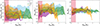 |
Fig. D.2. Properties of the PAH clouds vs galactocentric radius per environment for all the clouds in the 66 galaxies: Σmol (left), Mmol (middle), and Req (right). The running median property per galaxy median (dashed line) is plotted for a bin width of 0.2 Re. The shaded region represents the 84-50th and 50-16th percentiles of the medians per galaxy. The error bars on the median are the standard errors (1.253σ/ |

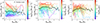 |
Fig. D.3. Properties of the PAH clouds vs galactocentric radius per environment for all the clouds in the 66 galaxies: Σmol (left), Mmol (middle), and Req (right). The running median property per galaxy median (dashed line) is plotted for a bin width of 0.2 Re. In each plot, the individual galaxy trends are color-coded by the median of the property. |
Here, we present the radial profiles per environment. In Sect. 5.4, we presented the global trends and showed that Req shows a flat profile and the Σmol radial profile is slightly decreasing. Fig. D.2 further shows that Req is also flat per environment with a slight decrease after 2 Re for interarm clouds. The Mmol and Σmol profiles generally show a decreasing trend per environment after 0.5 Re.
The individual-galaxy radial profiles are shown in Fig. D.3. The trends largely vary per galaxy. However, the consensus is a decreasing Mmol and Σmol profile after 0.5 Re. Upon adding the flagged clouds or adopting another αCO prescription (e.g., only metallicity dependent, or a constant αCO), we notice a bump in the Mmol and Σmol profiles toward central regions due to higher αCO values and the addition of overlapping structure, which mostly affects central regions. This confirms a general declining Mmol and Σmol radial profiles.
D.3. Galaxy-by-galaxy mass spectra
 |
Fig. D.4. Normalized survival function fits for PAH clouds in different environments. The dashed black block curve represents the fit for all the clouds, and the other block curves are for all clouds in a specific environment, as labeled (i.e., bar in purple, spiral arm in light blue, interarm in green, and disk in yellow). The dashed curves, color-coded by sSFR, are the fits to the galaxy-by-galaxy per environment (depending on the block curves). |
D.4. Mass-radius relationship
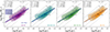 |
Fig. D.5. log(Mmol)-log(Req) scaling relation for the clouds in the different environments. Colored density contours represent 1, 2, and 3 σ contours in their corresponding galactic environments, and the stars show the median values. The solid line in each plot is a linear regression for the clouds in a specific environment. The slope and intercept are given by m and n, respectively, and the correlation coefficient is given by r. The 2D histogram of the full sample is shown in gray. The blue line represents the linear regression for the clouds regardless of environment, and its fit parameters are represented in the blue box in the leftmost plot. The diagonal dotted lines represent constant Σmol lines at 100, 101, 102, and 103 M⊙ pc−2. |
The mass-radius relationship is shown in Fig. D.5 for the full Global cloud sample and the clouds per galactic environment. We compare the distribution to constant Σmol lines plotted and notice that a significant number of clouds exist at the typical observed Σmol ≤10 M⊙ pc−2, which corresponds to the peak of the lognormal column density distribution in the F770W band (∼1021 cm−2 ; Pathak et al. 2024). However, these clouds appear to span over all Req, similar to the clouds in regions above 10 M⊙ pc−2.
We fit a linear regression using linmix12 and take the median values of the fit parameters with errors as 84th - 50th and 50th - 16th percentiles. Generally, the slopes are similar in each galactic environment, and the spiral arm clouds are located at higher Mmol and Σmol values compared to the other environments (see Fig. D.5).
D.5. Correlations
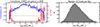 |
Fig. D.6. Left: Spearman correlation coefficient (solid blue) and the corresponding probability values (solid red) between the sum of the binned cloud Mmol ( |

D.6. The scaling parameter
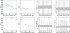 |
Fig. D.7. Top row: Variation in the total number of clouds (N), flux within the clouds relative to the total flux (fall), equivalent radius of the clouds (Req), and molecular mass of the clouds (Mmol) as a function of varying radius scaling parameter (from 50 to 150 pc), assuming a constant Mmol scaling parameter of 5 × 10⁶ M⊙. Bottom row: Same as the top row, but with a varying Mmol scaling parameter between 105 and 108 M⊙, assuming a constant Req scaling parameter of 100 pc. The box plots represent the median and the interquartile range of their distributions, and the whiskers cover the rest of the distribution. All results are shown for NGC 1385. |
We tested how changing the scaling parameters in SCIMES for both Req and Mmol affects the way clouds are grouped, as well as how it impacts the size and mass distributions of the clouds. Figure D.7 shows that when we keep the Mmol scaling parameter at 5 × 10⁶ M⊙ and adjust the Req parameter between 50 and 150 pc, the total number of identified clouds changes by only about 3 % compared to our default setup, where Req is set at 100 pc and Mmol at 5 × 10⁶ M⊙. Even with this slight change in cloud numbers, the recovered flux and the distributions of Req and Mmol remain steady and follow the same general pattern.
When we keep Req fixed at 100 pc and instead vary the Mmol scaling parameter, the results stay consistent for clouds with masses above 106 M⊙, similar to what we saw when adjusting Req. However, setting the Mmol parameter too low (below 105 M⊙) or too high (over 108 M⊙) causes clustering problems. In these cases, the algorithm either picks up too few clusters, leaving behind massive structures that stretch across large regions, for example spiral arms (as seen with the 105 M⊙ case), or it allows these large regions to stay grouped because of the high scaling parameter.
D.7. Cloud radius prescription
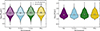 |
Fig. D.8. Left: PAH cloud radius using the area of the cloud across different galactic environments. The beam-deconvolved radii are represented in the colored violins, and the nondeconvolved radii are shown in the transparent violins. The dashed and dotted lines are the medians of the deconvolved and nondeconvolved radii, respectively. Right: Radii of the clouds using second-moment measurements across different galactic environments. The dashed line is the second-moment radius median. |
The radius of the clouds can be assessed by two different measurements (see Fig. D.8 and Sect. 4). In this paper, we recommend the usage of Req as it could be directly inferred from the number of pixels within the clouds. We applied the beam deconvolution using a Gaussian beam, which led to some inaccuracies in the measurement of Req. However, this is an effort to remove the beam contribution. The median Req across the sample is  pc (medians with the 84th - 50th percentile and 50th - 16th percentile displayed in superscript and subscript for the full cloud distribution). For comparison, the median nondeconvolved radius is
  pc, and the median radius based on the second spatial moment is
  pc. We emphasize that our main results are robust to the choice of radius definition, and adopting any of these estimates does not alter the conclusions of our analysis.
D.8. F1130W and F770W comparison
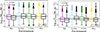 |
Fig. D.9. Mmol and Σmol of the PAH clouds according to F1130W (colored) and F770W (black) in 20 galaxies. The dotted line is the median property for the F770W band, and the dashed line is the median property for the F1130W band. The total number of clouds is displayed in the lower right of the plots. |
The results presented in our analysis are consistent when considering another band. In this section, we compare cloud properties using both F770W and F1130W bands at homogenized physical resolutions for the 20 galaxies that have F1130W observations in the PHANGS-JWST sample. The difference between the molecular properties of the clouds extracted using Chown et al. (2025) prescriptions between the F770W and F1130W (Eq. C2 in Chown et al. 2025) bands is only ∼0.1 dex as seen in Fig. D.9. This minimal effect discrepancy between the bands could be due to stellar continuum emission that plays a minimal role in the F1130W, hence it is not subtracted. It is worth noting, however, that the F1130W band also traces more neutral PAHs than the F770W band, which traces ionized PAHs mainly. This could create further differences toward the central regions of the galaxies.
All Tables
Survival function parameters (σ, s) for the Global sample of clouds, per galactic environment, and galaxy-by-galaxy (σgal, sgal).
Spearman correlation coefficients (r) and p-values (p) between the scale parameter of the lognormal distribution sgal, the shape parameter σgal, the total mass within clouds (∑Mmol), and various galactic and/or cloud parameters across the 66 galaxies.
Pearson χ2 and fractional difference statistical tests for the extreme cloud subsamples.
All Figures
|
Fig. 1. A zoomed-in view of NGC1566, one of the 66 galaxies. Left: Continuum-subtracted intensity image of the galaxy in the F770W MIRI band. The 2σ CO intensity contours from PHANGS-ALMA are represented in black. Right: PAH cloud structures identified by SCIMES color-coded by their F770W intensities. The green, blue, and red contours indicate the spiral arm, bar, and central region masks, respectively. The interarm region in this case consists of the remaining clouds that are not enclosed by the contours. The number of PAH clouds identified in this galaxy is represented in the bottom right. The color bar at the top of the image shows the 7.7 μm intensity range of the identified clouds. |
| In the text | |
|
Fig. 2. GMCs in NGC0628. CO-identified GMCs using CPROPS are shown as red ellipses (Hughes et al., in prep.), and the 7.7 μm identified PAH clouds using SCIMES are shown in the background in different colors. A zoomed-in view of the central region is shown in the inset (upper right corner); it focuses on the structures identified by both PAH and CO. This image highlights the resolution advantage of PAH clouds and the better sensitivity compared to CO, which allows the detection of fainter and smaller clouds where CO is not detected. |
| In the text | |
|
Fig. 3. Box plots with quantiles and outliers comparing the Σmol, R (left), cloud radius (middle), and cloud area (AR; right) distributions of cross-matched PAHs at 30 pc physical resolution and CO clouds at 90 pc in a subsample of 27 galaxies. The colored boxes represent the PAH cloud property distributions without overlapping clouds. The black boxes represent the property distributions of the cross-matched CO clouds. The dashed and dotted horizontal lines represent the median property of the full sample of CO clouds and PAH clouds, respectively. |
| In the text | |
|
Fig. 4. Violin plots showing the distribution and medians of Σmol in each galactic environment for the full sample of PAH clouds (colored) and the 77 844 clouds without overlap (transparent) in the 66 galaxies. The dashed line represents the median Σmol for the full PAH cloud sample. |
| In the text | |
|
Fig. 5. Left: Cumulative distributions of the molecular mass surface densities from the full cloud sample. The different colors represent the different environments. The y-axis is the fraction of clouds with a surface density greater than a given value. All distributions are normalized by the total area of their specific environment, A. Middle: Same as the left plot, but only considering barred spiral galaxies and excluding disks. Right: Same as the left plot, but only considering barred disk galaxies and excluding spirals. We removed the central region from the PDFs due to overlapping cloud bias. |
| In the text | |
|
Fig. 6. Cumulative distributions of the molecular mass surface densities from the full cloud sample. The different colors represent the different environments. The y-axis is the fraction of clouds with a surface density greater than a given value. All distributions are normalized by the total number of clouds in their corresponding environment, Ntot. We removed the central region from the PDFs due to overlapping cloud bias. |
| In the text | |
|
Fig. 7. Mass spectra for the PAH clouds in different environments, as labeled in each plot. The dashed black curves show the survival function fits. The fit parameters are displayed in the bottom left corner of each figure, where σ is the shape parameter and s is the scale parameter. The gray region represents the Poisson errors on the counts |
| In the text | |
|
Fig. 8. Normalized survival function fits for PAH clouds per galaxy. The dark blue dashed line represents the global fit to the entire sample. The background thin dashed lines are color-coded by specific star formation rate (sSFR) and show the global fits to each galaxy. |
| In the text | |
|
Fig. 9. Properties of the PAH clouds vs Rgal for all the clouds in the 66 galaxies: Σmol of the cloud (left), Req (middle), and the total number of galaxies contributing to a specific bin (right). The running galaxy median (filled black circles) is plotted for a bin width of 0.2 Re. The gray-shaded region represents the interquartile range of the medians per galaxy. The error bars on the median are the standard errors (1.253σ/ |
| In the text | |
|
Fig. D.1. Summary of galaxy-by-galaxy properties. The plots are available at https://zenodo.org/records/15428261. Top left: Continuum-subtracted images of the galaxy. Top right: PAH clouds identified using SCIMES. The flagged clouds are in gray, unflagged in green, and PAH clouds with CO cloud counterparts in red. Middle left:Σmol violin plots per galactic environment for the specific galaxy (transparent), and the full sample (colored). The median values and number of PAH clouds per environment are also represented in the plot. Middle center: log(Mmol )-log(Req) scaling relation for the PAH clouds in the galaxy (blue), clouds per galactic environment in the galaxy (see colors in plot), and for the full sample (black). The median values are also represented in the plot per galactic environment. Middle right: Global mass spectra (black), galaxy-specific mass spectra (blue), and per galactic environment in the galaxy. The fit values for the galaxy-specific mass spectra are displayed in the plot. Bottom:Σmol (left), Mmol (center), and Req (right) as a function of Rgal. A scatterplot of the PAH clouds, color-coded by the density of clouds, is also represented. The running galaxy median (filled blue circles) is plotted for a bin width of 0.1 Re. The gray-shaded region represents the interquartile range of the medians per galaxy. The error bars on the median are the standard errors (1.253σ/ |
|
| In the text | |
|
Fig. D.2. Properties of the PAH clouds vs galactocentric radius per environment for all the clouds in the 66 galaxies: Σmol (left), Mmol (middle), and Req (right). The running median property per galaxy median (dashed line) is plotted for a bin width of 0.2 Re. The shaded region represents the 84-50th and 50-16th percentiles of the medians per galaxy. The error bars on the median are the standard errors (1.253σ/ |
| In the text | |
|
Fig. D.3. Properties of the PAH clouds vs galactocentric radius per environment for all the clouds in the 66 galaxies: Σmol (left), Mmol (middle), and Req (right). The running median property per galaxy median (dashed line) is plotted for a bin width of 0.2 Re. In each plot, the individual galaxy trends are color-coded by the median of the property. |
| In the text | |
|
Fig. D.4. Normalized survival function fits for PAH clouds in different environments. The dashed black block curve represents the fit for all the clouds, and the other block curves are for all clouds in a specific environment, as labeled (i.e., bar in purple, spiral arm in light blue, interarm in green, and disk in yellow). The dashed curves, color-coded by sSFR, are the fits to the galaxy-by-galaxy per environment (depending on the block curves). |
| In the text | |
|
Fig. D.5. log(Mmol)-log(Req) scaling relation for the clouds in the different environments. Colored density contours represent 1, 2, and 3 σ contours in their corresponding galactic environments, and the stars show the median values. The solid line in each plot is a linear regression for the clouds in a specific environment. The slope and intercept are given by m and n, respectively, and the correlation coefficient is given by r. The 2D histogram of the full sample is shown in gray. The blue line represents the linear regression for the clouds regardless of environment, and its fit parameters are represented in the blue box in the leftmost plot. The diagonal dotted lines represent constant Σmol lines at 100, 101, 102, and 103 M⊙ pc−2. |
| In the text | |
|
Fig. D.6. Left: Spearman correlation coefficient (solid blue) and the corresponding probability values (solid red) between the sum of the binned cloud Mmol ( |
| In the text | |
|
Fig. D.7. Top row: Variation in the total number of clouds (N), flux within the clouds relative to the total flux (fall), equivalent radius of the clouds (Req), and molecular mass of the clouds (Mmol) as a function of varying radius scaling parameter (from 50 to 150 pc), assuming a constant Mmol scaling parameter of 5 × 10⁶ M⊙. Bottom row: Same as the top row, but with a varying Mmol scaling parameter between 105 and 108 M⊙, assuming a constant Req scaling parameter of 100 pc. The box plots represent the median and the interquartile range of their distributions, and the whiskers cover the rest of the distribution. All results are shown for NGC 1385. |
| In the text | |
|
Fig. D.8. Left: PAH cloud radius using the area of the cloud across different galactic environments. The beam-deconvolved radii are represented in the colored violins, and the nondeconvolved radii are shown in the transparent violins. The dashed and dotted lines are the medians of the deconvolved and nondeconvolved radii, respectively. Right: Radii of the clouds using second-moment measurements across different galactic environments. The dashed line is the second-moment radius median. |
| In the text | |
|
Fig. D.9. Mmol and Σmol of the PAH clouds according to F1130W (colored) and F770W (black) in 20 galaxies. The dotted line is the median property for the F770W band, and the dashed line is the median property for the F1130W band. The total number of clouds is displayed in the lower right of the plots. |
| In the text | |
Current usage metrics show cumulative count of Article Views (full-text article views including HTML views, PDF and ePub downloads, according to the available data) and Abstracts Views on Vision4Press platform.
Data correspond to usage on the plateform after 2015. The current usage metrics is available 48-96 hours after online publication and is updated daily on week days.
Initial download of the metrics may take a while.