| Issue |
A&A
Volume 706, February 2026
|
|
|---|---|---|
| Article Number | A245 | |
| Number of page(s) | 15 | |
| Section | Extragalactic astronomy | |
| DOI | https://doi.org/10.1051/0004-6361/202556357 | |
| Published online | 13 February 2026 | |
A group of merging galaxies falling into Abell 2142
1
LUX, Observatoire de Paris, Sorbonne Université, Université PSL, CNRS F-75014 Paris, France
2
Astronomisches Rechen-Institut, Zentrum für Astronomie der Universität Heidelberg Mönchhofstr. 12–14 69120 Heidelberg, Germany
3
Sternberg Astronomical Institute, Moscow M.V. Lomonosov State University, Universitetskij Pr. 13 Moscow 119234, Russia
4
Collège de France 11 Place Marcelin Berthelot 75005 Paris, France
★ Corresponding author: This email address is being protected from spambots. You need JavaScript enabled to view it.
Received:
10
July
2025
Accepted:
30
December
2025
Abstract
Galaxy clusters produce a very hostile environment for galaxies: their gas gets stripped by ram pressure, they undergo galaxy interactions, and their star formation is quenched. Clusters, like Abell 2142, grow not only through galaxy accretion but also through galaxy group infall. Our goal was to study the physical and dynamical state of the most conspicuous infalling group, which is located at a projected distance of 1.3 Mpc from the Abell 2142 centre. The galaxy group G is the leading edge of a spectacular 700 kpc long X-ray tail of hot gas stripped by ram pressure. The infalling galaxies are not quenched yet and are ideal objects for studying the transformation processes due to the cluster environment. We used integral field spectroscopy from MaNGA to derive stellar and gas kinematics, and MegaCam for photometry. Stellar populations (with age and metallicity) were obtained through full-spectrum fitting using NBURSTS. The gas kinematics and excitation were derived from the line emission of Hα, [N II], [O III], and Hβ. The group contains four galaxies, two of which are merging and partly superposed on the line of sight. With a simple parametric model for each velocity field, we succeeded in disentangling the contribution of each galaxy and derived their physical state and kinematics. They are primarily rotating discs, but perturbations and out-of-equilibrium gas manifest as regions of elevated dispersion and as tidal tails and loops of intra-group material. All galaxies show sustained star formation, with a global star formation rate of 42 M⊙/yr. We conclude that the long X-ray tail must have come from the hot intra-group medium, present before the group infall, and does not correspond to the ram-pressure stripping of the galaxy gas. Ongoing interactions between the group members enhance the star formation activity by inducing mixing of dense gas from their gas-rich galactic discs.
Key words: techniques: imaging spectroscopy / galaxies: clusters: general / galaxies: groups: general / galaxies: interactions / galaxies: star formation
© The Authors 2026
 Open Access article, published by EDP Sciences, under the terms of the Creative Commons Attribution License (https://creativecommons.org/licenses/by/4.0), which permits unrestricted use, distribution, and reproduction in any medium, provided the original work is properly cited.
This article is published in open access under the Subscribe to Open model. This email address is being protected from spambots. You need JavaScript enabled to view it. to support open access publication.
1. Introduction
Galaxy clusters are the largest gravitationally bound structures in the Universe; they are formed through the non-linear growth of primordial density fluctuations (Vikhlinin et al. 2014). These massive assemblies of galaxies are dominated by dark matter and hot gas, the latter of which emits X-ray radiation (Bahcall 1977; Bykov et al. 2019). They evolve slowly and retain important clues about the Universe’s formation through the ongoing accretion of galaxies (e.g. Springel et al. 2006). It is well established that environment significantly influences galaxy evolution, with galaxies in high-density regions undergoing markedly different evolutionary paths than those in lower-density environments (Pasquali 2015; Mateus et al. 2007). Galaxies within clusters tend to be redder, more compact, and have larger Sérsic indices compared to their counterparts in the field (Pranger et al. 2017). They also experience gas depletion and reduced star formation rates (SFRs), a result of the dense cluster environment (Boselli & Gavazzi 2006; Bower & Balogh 2004).
One of the key processes affecting galaxies as they fall into a cluster is ram pressure stripping (RPS). As galaxies move through the hot intracluster medium (ICM), the pressure exerted by the ICM can strip away their gas, though the stars are largely unaffected (Gunn & Gott 1972; Fillingham et al. 2016; Steinhauser et al. 2016). Galaxies with RPS tails, commonly known as jellyfish galaxies, exhibit this gas removal in various phases, for example neutral hydrogen (Chung et al. 2007; Scott et al. 2012) and molecular gas (such as CO; Jáchym et al. 2013, 2014, 2017); it is even visible in X-ray observations (Sun et al. 2006). The process removes gas in layers, akin to peeling onion skins, with the hot diffuse gas being stripped very efficiently and molecular gas remaining more resistant (Bekki 2009; Hausammann et al. 2019). In high-density environments, RPS can significantly deplete the interstellar medium (ISM) of the galaxy, suppressing star formation (Boselli et al. 2022, and references therein). While observations show that SFRs can be high in stripped tails because gas is removed from the disc onto the tail, what is surprising is the temporary boost in star formation within the disc itself, as the increased pressure compresses the ISM gas into stars before stripping begins (Vulcani et al. 2018).
While individual galaxies undergo significant transformation as they move through the cluster environment, many galaxies do not fall into clusters in isolation. Recent simulations by Kuchner et al. (2022) suggest that about 12% of the galaxies that fall into clusters arrive in groups, which are smaller gravitationally bound systems containing a few to dozens of galaxies. Galaxy groups are the sites of complex interactions, which transform galaxies even before they enter a cluster (Choque-Challapa et al. 2019; Lopes et al. 2024); this is called ‘pre-processing’ (Bianconi et al. 2018) and involves gravitational perturbations, enhanced gas stripping (Kleiner et al. 2021), and an increased likelihood of mergers within galaxies (Vijayaraghavan & Ricker 2013; Benavides et al. 2020). These mergers can significantly influence star formation, sometimes triggering bursts of activity (Sanders et al. 1988; Bekki 1999; Li et al. 2008) or, conversely, leading to quenching.
Both galaxy mergers (Comerford et al. 2024) and RPS are known to trigger active galactic nuclei (AGNs). Peluso et al. (2022) find a significantly higher AGN fraction in ram-pressure-stripped galaxies, especially massive ones, aligning with Ricarte et al. (2020), who noted that RPS enhances black hole accretion in massive galaxies during pericentric passage but suppresses it in less massive ones. Poggianti et al. (2017) report a high incidence of AGNs among extreme jellyfish galaxies, suggesting that ram pressure funnels gas towards galactic centres to trigger AGN activity. Marshall et al. (2018) developed a model that indicates that this triggering occurs within a specific range of ram pressures (Pram = 10−14 − 10−13 Pa).
Such group–cluster interactions are particularly evident in systems like Abell 2142, which is at z = 0.0894 (Bilton & Pimbblet 2018), where the infall of galaxy groups drives much of the cluster’s ongoing evolution. Its properties are summarised in Table 1. Previous studies, such as those by Buote & Tsai (1996) using ROSAT X-ray imagery, argue that A2142 has reached an advanced stage of merger, a notion further explored by Markevitch et al. (2000), who identified A2142 as a merger involving two subclusters based on Chandra observations. From optical (Subaru) and X-ray (Chandra) observations, Okabe & Umetsu (2008) detected a complex core region marked by two cold fronts, supporting the merger scenario.
Properties of the galaxy cluster Abell 2142.
Liu et al. (2018) spectroscopically identified 868 galaxy members within 3.5 Mpc, unveiling substructures indicative of ongoing merging activity. This galactic ensemble serves as an ideal testing ground for numerical simulations and dark matter assembly (e.g. Munari et al. 2014, 2016). Nested within a collapsing super-cluster (Einasto et al. 2015, 2020), A2142 hosts detached long filaments that seamlessly connect to the cosmic web (see also Poopakun & Kriwattanawong 2019). Recently, with the advent of LOFAR radio data, Bruno et al. (2023) unveiled a three-component giant radio halo within A2142.
Numerous groups are falling into A2142 (Einasto et al. 2018). SDSS J155850.44+272323.9 (at z = 0.0935) is the main galaxy of a gas-rich infalling galaxy group; it is referred to as Group G and was studied via X-rays by Eckert et al. (2014, 2017). This galaxy group, located at around 1.3 Mpc north-east of the centre of Abell 2142 (i.e. Rgg, the projected distance of the galaxy group with respect to the cluster centre), has been caught before its quenching and exhibits the highest star formation activity (40 M⊙/yr; Salim et al. 2016) of all the groups in the cluster. It is located at the tip of a spectacular 700 kpc long X-ray tail typical of hot gas stripped by RPS. From XMM-Newton observations, Eckert et al. (2014) estimated that this group (with a mass of a few times 1013 M⊙) is falling into the cluster with a relative velocity of about 1200 km/s, and that 95% of the group’s hot gas was expelled more than 600 Myr ago into the tail; the remaining 5% is still present. Deep Chandra observations of the group revealed significant AGN activity in two of the galaxies (marked in Fig. 1 as Galaxy a and Galaxy b) with X-ray luminosities of (2.4 ± 0.3)×1042 erg s−1 and (3.0 ± 0.4)×1042 erg s−1, respectively, in the [2 − 10] keV band (Eckert et al. 2017). They also identified a complex morphology in the tail characterised by an abrupt flaring beyond 250 kpc and a drop in metallicity beyond 300 kpc. Their study highlighted the role of magnetic draping and slow gas interactions with the ICM in shaping the tail, with the structure showing signs of turbulence and suppressed thermal conduction.
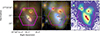 |
Fig. 1. SDSS (Data Release 12) gri image (left), MegaPipe ugr image (centre), and unsharp masking of the MegaPipe r-band image (right), with the MaNGA field of view overlaid in magenta. The three main stellar regions are segregated and marked as (a, b, c) on the SDSS image. The centres of the regions, with a subdivision of the a region into two galaxies, are shown on the MegaPipe images. |
In this paper we explore the kinematics of this complex system with SDSS Mapping Nearby Galaxies at Apache Point Observatory (MaNGA) data. In Sect. 2 we describe the data. In Sect. 3 we outline the stellar analysis, and in Sect. 4 we analyse the gas in the system. In Sect. 5 we discuss our results, and we present our conclusions in Sect. 6. Throughout the paper we assume a Λ cold dark matter cosmology with Ωm = 0.3, ΩΛ = 0.7, and H0 = 70 km s−1/Mpc.
2. Data description and characteristics
2.1. Optical integral field unit data from MaNGA
This galaxy group (MaNGA ID: 1-265404, plateifu = 9094–1902) was observed as part of the MaNGA survey (Bundy et al. 2015) on 17 April 2018. The spectra were acquired through the MaNGA instrument (Drory et al. 2015) mounted on the Sloan Foundation 2.5-meter Telescope, which is located at the Apache Point Observatory in New Mexico, USA. The MaNGA Data Analysis Pipeline (DAP) utilises the MILESHC template (Westfall et al. 2019) for the stellar kinematics and MaSTAR stellar library to obtain the emission lines. The data products include a 3D reduced data cube and 2D maps of emission lines properties.
The centre of the data cubes is located at RA = 15h58m50.4s, Dec = 27° 23′23.9″, which does not necessarily coincide with the centre of the galaxy group. The dimensions of the data cubes are 32 × 32 × 4563; the first two values correspond to the spatial dimensions and the third to the wavelength dimension. The spectral data are stored in the ‘FLUX’ extension, with each pixel containing information about the specific intensity in units of 1 × 10⁻¹⁷ ergs−1 cm−2 Å−1 spaxel−1. The spectral cube covers a broad wavelength range, from 3600−10 300 Å at R ∼ 2000. The pixel size is 0.5 arcsec, which corresponds to 0.87 kpc at z = 0.0935. The spatial full width at half maximum (FWHM) of the reconstructed Gaussian point spread function (PSF) in the g or r bands is of the order of 2.6 arcsec (4.5 kpc) and the spectral FWHM resolution ranges from 250 km/s on the blue end to 150 km/s on the red end.
2.2. MegaCam/MegaPipe ugr photometry
We used archival data from MegaCam, a state-of-the-art wide-field imaging facility at the Canada-France-Hawaii Telescope (CFHT). MegaCam has a 0.187-arcsec pixel size and accurate photometric calibrations up to 0.03 mag. The median seeing at centre is 0.77″ in the g and 0.66″ in the i band1. The data from the MegaCam Image Stacking Pipeline (MegaPipe; Gwyn 2008), utilising first-generation broadband filters, ugr, were used to create a combined red-green-blue image (Fig. 1), photometric modelling (Fig. 2), and to perform unsharp masking (Fig. 1).
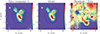 |
Fig. 2. Photometric modelling of the CFHT MegaPipe r-band image using GALFIT. Blue hexagons show the MaNGA field of view, ‘x’ symbols indicate the centres of the ‘core’ components, dots near the c and b components indicate the centres of the ‘outskirts’ components, and the dot between a1 and a2 is the centre of the‘bridge’ between them (see Sect. 3.1.2). Dashed ellipses show the effective radius of the most ‘extended’ component of each galaxy, based on the parameters from Table 2. Third panel shows the residuals-to-data ratio. The colour bar unit is proportional to the analogue-to-digital unit. |
At first glance, we observe three main stellar structures in the left panel of Fig. 1. However, upon closer inspection, we notice two distinct colours in the SDSS (Data Release 12, Alam et al. 2015) image of the central galaxy: the northern part of the galaxy (a) appears bluer than its southern part. To investigate this further, we applied a Gaussian filter with a standard deviation of σ = 0.75 to enforce a common effective resolution and generated a Lupton red-green-blue image (Lupton et al. 2004, central panel of Fig. 1) using the MegaPipe cutouts of the r, g, and u bands as the red, green, and blue channels, respectively. This figure depicts that galaxies (b) and (c) are redder than the central galaxy, which can be attributed to either the older stellar population or the presence of dust. Galaxy (c) seems to be merging with a bluer galaxy, which, however, is situated outside of the MaNGA field of view.
To investigate potential substructures within the central galaxy, we applied a Gaussian convolution with a standard deviation of 0.5 to the original image, using the Gaussian2DKernel from Astropy. The resulting convolved image was then subtracted from the original data, scaled appropriately, and adjusted for dynamic range. This is equivalent to unsharp masking. Two distinct features (henceforth referred to as a1 and a2) become evident in the central region, revealing two galaxies (in Fig. 1) instead of the one previously perceived. Moreover, the tidal tails and their directions are enhanced in this image.
We performed a GALFIT analysis (Peng et al. 2002, 2010) using the MegaPipe r-band image. It was the reddest band with the best seeing (0.71″) for correct decomposition and obtaining stellar luminosity. The merging group is complex and cannot be easily modelled with symmetric and stationary components, as it contains star-forming regions, dust lanes, tidal tails, and shells. In our analysis, we assumed that each galaxy consists of a central ‘core’, while galaxies b and c also have extended ‘outskirts’ components. The ‘core’ components were modelled using a Sérsic profile (centres of which are represented by crosses in Fig. 2), while the extended components were fitted with an exponential disc profile (centres of which are represented by dots in Fig. 2). For galaxies a1 and a2, we added a compact exponential disc that acts as a ‘bridge’ between them and provides a good fit. Galaxies b and c exhibited off-centred components, possibly due to ram pressure or other external factors. The final parameters of the galaxies are provided in Table 2, and the image, best-fit model, and residuals are shown in Fig. 2.
2.3. Subaru photometry
Subaru images in the g and r bands are shown in Appendix A. While some central pixels are blank, thereby precluding their use in our analysis, the images provide an even better view of structures such as tidal tails and bridges.
3. Stellar analysis and a first glance at the gas component
3.1. Stellar populations
One of our objectives was to estimate the stellar masses of the system’s components. Using GALFIT, we were able to decompose the photometric information of the system into its individual components and determine their luminosities. However, to derive the stellar mass, we require the mass-to-light ratio (M/L), which depends on the properties of the stellar populations. These properties can be determined using a full-spectrum fitting with a two-component technique. Before applying this method, several preliminary steps are necessary.
3.1.1. One-component analysis
The first step involves performing a full-spectrum fitting using a one-component model, i.e. a single stellar population (SSP) model, with NBURSTS (Chilingarian et al. 2007a,b), in order to estimate the average properties of the stellar populations, including the age (TSSP) and metallicity ([Z/H]SSP), as well as the stellar and gas kinematics, such as velocity (V) and velocity dispersion (σ). For this analysis, we employed NBURSTS with a grid of SSP models from the E-MILES library (Vazdekis et al. 2016).
The general formulas of NBURSTS are
 (1)
(1)
 (2)
(2)
Here, Pnmult denotes the multiplicative continuum in the form of a Legendre polynomial, while Nst and Nem represent the number of stellar components and emission lines, respectively. The terms pst and pem refer to the contributions of the stellar component (ranging from 0 to 1, ∑Nstpst = 1) and the emission line (the flux of the line). The symbols Tst and Tem denote models for the stellar and emission line components, and ℒst and ℒem represent the convolved parametrised line-of-sight velocity distributions (LOSVDs) with the spectrograph’s line spread function. In Eq. (2), pλ is the mask for good wavelengths, Fλ represents the observed spectrum, and ΔFλ is the error associated with the spectrum.
During each model evaluation in the χ2-minimisation process (Eq. 2), the stellar population spectrum is interpolated from the model grid based on the given age (TSSP) and metallicity ([Z/H]SSP) values. The interpolated spectrum is then convolved with the stellar LOSVD, which in our case is parametrised by a pure Gaussian. Additionally, the spectrum is multiplied by a polynomial continuum to account for the difference between the model and observed spectral shapes, which arises from imperfect spectral sensitivity calibration and the effects of dust extinction. For this, we employed multiplicative Legendre polynomials of the 19th degree (1 degree per each 150 − 200 Å of wavelength range and an odd degree is required). The model also includes a set of strong emission lines (Hγ, Hβ, [O III], [O I], [N II], Hα, [S II], etc.) possessing the same Gaussian kinematics but are treated independently from the stellar kinematics. These emission lines are additive components whose weight, i.e. emission line fluxes, are determined as part of a linear problem solved at each iteration of the non-linear minimisation loop. Prior to the main minimisation process, both the emission line templates and the grid of stellar population templates were pre-convolved with the wavelength-dependent instrumental resolution.
The main results of this analysis are shown in Figs. 3 and 4, applied to the datacubes after Voronoi binning to a target signal-to-noise ratio (S/N) of approximately 20. With this procedure, we confirmed the stellar and gas kinematic maps provided by MaNGA DAP (Westfall et al. 2019). We also obtained the stellar population parameters TSSP and [Z/H]SSP, along with the stellar spectra unconvolved with a parametric Gaussian LOSVD, in each spatial bin.
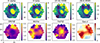 |
Fig. 3. Emission line maps from NBURSTS single Gaussian fits. The main emission lines (Hα, Hβ, [O III]5008, and [N II]6585) are displayed in arbitrary units; the gas velocity dispersions fixed to all lines are in km/s. The x and y coordinates are in MaNGA pixels of 0.4″. |
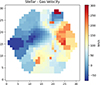 |
Fig. 4. Difference between the stellar and gas velocity. |
From Fig. 3 we can draw several conclusions regarding the star-forming regions and the galaxies involved. The high Hα/Hβ ratio observed at the centre suggests significant dust attenuation, indicating a rich star formation activity. Additionally, the very high [O III]/Hβ ratio supports the previous X-ray identification of (b) as an AGN (following the line ratio diagnostics of Baldwin et al. 1981) while Galaxy (a1) seems to be obscured by dust, impacting its AGN visibility. Furthermore, the high-velocity dispersion in the central region aligns with expectations; however, the anomalous dispersions noted in the bottom-left and top-right areas may be indicative of some unknown perturbations affecting the dynamics within this system and/or to the superposition of lines at different peculiar velocities. A velocity difference of 300 km/s between the gas and stellar components seen in Fig. 4, combined with a high SFR and the presence of an AGN, may indicate that outflows from the AGN and feedback from star formation processes are driving the observed kinematic features.
3.1.2. Two-component analysis
To investigate the two-component stellar kinematics using NBURSTS in our sample and perform full-spectrum fitting with two stellar components, an accurate initial approximation of the kinematics of the components was required and we employed a non-parametric LOSVD recovery approach, successfully used in previous studies (e.g. Katkov et al. 2016; Kasparova et al. 2020; Katkov et al. 2024), with a detailed description provided in Gasymov & Katkov (2024). The key concept of this method is to find a convolution kernel such that, when convolved with the original stellar spectrum, the result best reproduces the observed spectra (see Fig. B.1). In the previous step, this kernel was parametrised as a pure Gaussian, but in this step we solved an ill-posed linear problem to recover its complex shape. This problem was addressed using a least-squares method, with additional L2 (Tikhonov) and ‘edge’ regularisation to smooth the solution and suppress spurious high-velocity peaks due to the limited S/N.
As shown in Fig. B.2, the solution is a vector of the LOSVD for each spatial bin, which allows us to trace the 3D kinematics of the system (in X-Y-V coordinates). In particular, the spaxels in the ‘merging’ regions reveal prominent two- or three-component structures, providing clear evidence of distinct kinematic behaviour in these galaxies, which cannot be accurately described by a single Gaussian parametric LOSVD. This multi-component structure enabled us to model the relative systemic velocities between the galaxies.
We selected the regions corresponding to components a2, b, and c (Figs. 5 and B.2) and assumed Gaussian kinematics for these components within the designated circular regions, defined in Fig. B.2. Using one-, two-, and three-Gaussian models in corresponding spaxels, we then examined the kinematic maps of each galaxy. These maps exhibit a consistent rotation pattern, which we modelled using a circular rotation model:
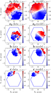 |
Fig. 5. Kinematical modelling of the stellar recovered LOSVD. The panels show the velocity maps of the different components and their corresponding models (see Sect. 3.1.2). Blue hexagons show the field of view covered by the MaNGA observations. |
 (3)
(3)
![Mathematical equation: $$ \begin{aligned}&V_0(r) = V_{\rm max} \tanh \left[\pi \cdot (|R|/R_0)\right]. \end{aligned} $$](/articles/aa/full_html/2026/02/aa56357-25/aa56357-25-eq4.gif) (4)
(4)
We fixed the inclinations (i) from b/a ratios by modelling the system as an oblate spheroid with an intrinsic axis ratio q0 of 0.2, so that the inclination i satisfies: cos2i = ((b/a)2 − q02)/(1 − q02), (Hubble 1926). We fixed R0 as Reff and central positions (x0, y0) derived from the extended components of the galaxies in the photometric analysis (Sect. 3.2). We used the parameters obtained for b and c galaxies from the exponential disc component because the Sérsic components are oriented close to face-on with small Reff. A known numerical issue of per-spaxel kinematic fit is peak ‘hopping’, i.e. artificial swapping of velocity components between neighbouring solutions. We solved this by a two-pass strategy. First, we performed an unconstrained fit using only rough systemic-velocity seeds (Va1, Va2, Vb, Vc = 0, 100, 500, 200 km s−1). Next, we modelled the velocity fields of the galaxies with Eqs. (3) and (4), re-fitted the LOSVDs using the initial approximation for the systemic velocities and the parameters Vmax, Vsys, and position angle (PA) were free. The final result is illustrated in Fig. B.2. The fitted stellar kinematics parameters are in good agreement with the gaseous kinematics (Tables 3 and 4).
Gas modelling.
The final step in determining the mass-to-light ratio is the estimation of the stellar population properties in each galaxy. As shown in Fig. B.2, some spaxels contain spectral contributions from multiple galaxies, which we could then divide using the previously derived kinematic initial approximations. In our analysis, we used the NBURSTS extension to perform spectral fitting with two stellar components. The key difference between this method and the one-component approach is that here the spectrum is modelled by the sum of two independent stellar populations, each with its own parametric LOSVD. This approach is particularly useful when there are significant differences in the velocities of the stellar populations and a comparable contribution to the galaxy luminosity, as is the case in systems with counter-rotation phenomenon (e.g. Katkov et al. 2013, 2016, 2024). Our merging system is another great example for applying this technique.
However, this method is highly sensitive to both the S/N and the accuracy of the initial parameter estimates, making it unsuitable for automatic fit in all spaxels. Hence, we selected several transitive (overlap) regions that feature comparable contributions from a1 and other galaxies. We then co-added these spaxels into a single bin to improve S/N and fitted the spectrum with two SSP components. The initial kinematic estimates were derived from the ‘circular’ rotation model, and these velocities were confirmed (Fig. B.2). The ages and metallicities with corresponding uncertainties of the stellar populations are listed in Table 2. Using these values, we computed the mass-to-light ratios in the SDSS r band.
3.2. Stellar masses
Stellar masses were derived from the luminosities of the galaxies obtained by the Galfit analysis from the MegaPipe r-band images, and the mass-to-light ratios. For the galaxies b and c, we combined the integrated magnitudes of their components, while for a1 and a2, we used the integrated magnitude of the Sérsic component. Assuming a luminosity distance of 428.6 Mpc (for z = 0.09353), we calculated the luminosities and stellar masses of all the galaxies (Table 2).
4. Gas analysis
To analyse the gas content within the group, we used the Hybrid-10 Model LOGCUBE made by the DAP from the MILESHC template for the stellar kinematics and the MaSTAR stellar library. Emission lines properties remain unbinned, while stellar properties are Voronoi binned to a S/N of approximately 10. We subtracted the fits of emission lines from the fits of the full spectra to obtain the stellar contribution to the spectra and we subtracted this contribution from the observed spectra to isolate the emission originating from the gas. We applied the correction provided by MaNGA for Galactic extinction, as a function of wavelength. The rest of the analysis described in this section is based on these spectra.
Figure 6 illustrates the large width of the [O III] emission line and the variety of shapes depending on the region. Given the width of emission lines, the Hα line is blended with the [N II] doublet, complicating the identification of individual components. While the DAP offers single-Gaussian fits for each emission line, significant residual spectra remain. These residuals call for a fitting of gas emission lines from a model with several galaxies. Residuals due to the presence of intra-group components, such as tidal tails, are expected to remain.
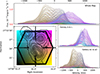 |
Fig. 6. Superposition of all [O III] lines from each pixel, colour-coded by the position of the pixel (as shown in the left panel). Bottom left: SDSS g-band image (black contours). The hexagon is the field of view of MaNGA. Top: Spectra of the whole map. Middle right: Top half of the field (i.e. the field above the dotted white line in the bottom-left panel), emphasising regions where galaxies b and c are present. Bottom right: Bottom half of the field, highlighting areas where galaxies a1 and a2 are situated. |
4.1. Kinematics of emission-line fitting from modelled galaxies
We modelled the gas kinematics through mock observations of four simulated galactic discs. Each disc was generated with particles having positions and velocities drawn from chosen distributions. We used a Miyamoto-Nagai density profile:
![Mathematical equation: $$ \begin{aligned} \rho _d(R,z) = \left(\dfrac{h^2 M}{4 \pi }\right) \dfrac{a R^2 + (a + 3\sqrt{z^2 + h^2}) (a + \sqrt{z^2 + h^2})^2}{\left[R^2 + (a + \sqrt{z^2 + h^2})^2\right]^{\frac{5}{2}} (z^2 + h^2)^{\frac{3}{2}}}, \end{aligned} $$](/articles/aa/full_html/2026/02/aa56357-25/aa56357-25-eq5.gif) (5)
(5)
where M is the total mass of the disc, a is a radial scale length, and h is a vertical scale length. a is set to 1 kpc for all discs, and h to 0.2 kpc. Discs are cut at four times their radial scale length (a). The impact of the exact profile on the modelling is diminished by the following fit in each spaxel, explained below. The rotation curve follows Eq. (4), as for the stellar disc. The disc is placed at the location of the core component found by the photometric fit2. Inclination, position angle, line-of-sight (LOS) systemic velocity, Vmax (plateau velocity of the rotation curve), R0 (transition radius of the rotation curve), and velocity dispersion (modelled with a single value for uniform and equal radial σR and azimuthal σϕ velocity dispersions and a uniform vertical velocity dispersion σz = 1/2σR) are all free parameters. Because of the high degeneracy, especially due to the presence of four galaxies in a region of only a few PSFs wide, we fitted these parameters of all discs by eye, guided by the values obtained for the stellar components.
We realised one mock cube per galaxy, by binning on-sky positions and LOS velocities of the simulated disc particles. LOS velocities are initially binned on channels of width 50 km/s and, for a given emission line, the simulated spectra are interpolated on the velocities obtained using the following conversion between wavelength λ and LOS velocity v:
 (6)
(6)
where zsource is the redshift and λ0 is the rest-frame wavelength in vacuum of the considered emission line, collected from the NIST Atomic Spectra Database3. At each simulated spaxel, we performed a convolution on velocities with a 1D Gaussian kernel with the dispersion of the MaNGA line-spread-function for the spaxel at the redshifted wavelength of the considered emission line (this dispersion is given in the MaNGA model cube). The planes corresponding to each simulated velocity channels are convolved by a circular Gaussian kernel of FWHM 2.6 arcsec, accounting for the MaNGA PSF in the g and r bands.
To fit an emission line from the four simulated mock cubes (with one mock cube per galaxy), we considered a varying contribution of each disc in each spaxel. For each disc i with a mock spectrum si, we fitted for the factors fi such that Σfisi matched the observed spectrum. As the fitting was performed after convolution of the mock cube by the MaNGA PSF, the fitted factors must not vary strongly on the area of the PSF for this approach to be physically valid (otherwise, the contribution of the gas of a given disc at a given location would be inconsistent from one spaxel to its neighbours on which it is smeared by the spatial convolution). We fitted the following emission lines: Hβ, [O III]5008, Hα+[N II] doublet, and the [S II] 6718, 6733 doublet.
We note that, without any clear inclination of disc components derived from the optical images, the large size of the MaNGA PSF compared to the galaxies makes the determination of the plateau rotation velocity and inclination of each disc completely degenerate in our modelling, because the iso-LOS-velocity curves of a disc are almost straight lines parallel to its minor axis. It is thus only possible to determine Vmax sin i. We computed the fits with couples of Vmax and inclination that are reasonable (we especially avoided unrealistically high rotation velocities) and used the inclination to draw the disc on the different figures.
Low-velocity gas (with a LOS velocity < 500 km/s) cannot be fitted by our model, as is visible in Fig. 8. This gas can be modelled by a broad kinematic component of velocity dispersion 500 km/s, spatially and kinematically centred on a2. This additional component is named a2 bis.
Figure C.1 shows observed and modelled spectra for one of the fitted emission lines, [O III]5008, stacked 16 by 16 at the corresponding on-sky locations, with the MegaPipe image as background. Figure 7 shows the moments for the [O III]5008 line. Figure 8 shows the emission lines stacked on the whole system in the observation and the models. Parameters used for the models are given in Table 4. While systemic velocities of galaxies b and c are close to the ones found in the stellar analysis, we obtain very different results for galaxies a1 and a2. Emission lines peak near 100 km/s at the location of the centre of a1, which makes us attribute this systemic velocity to a1. A neighbouring galaxy with a lower systemic velocity is needed to fit the emission lines, hence the systemic velocity −250 km/s attributed to a2. The differences in the results found by the stellar and gas analyses for these two galaxies reflect the high degeneracy of the system and the difficulties created by the low spatial resolution of the observation compared to the sizes of the galaxies.
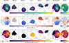 |
Fig. 7. Observations, models, and residuals of the flux, velocity, and velocity dispersion from the [O III]5008 Angstrom line. Models are shown for each component (Cols. 2 to 6) and for the five components together (Col. 7). Residuals (Col. 8) are the observation (Col. 1) minus the model (Col. 7). On the velocity maps of individual galaxies, iso-LOS velocity curves are represented in dashed (solid) black lines for values below (above) the systemic velocity of each galaxy. |
The velocity dispersions that are required to fit the spectra are especially large: 80 km/s for galaxies a1 and 100 km/s for galaxy a2, and as much as 250 km/s for galaxy b and 180 km/s for galaxy c. While the values for galaxies a1 and a2 may be due to kinematically hot gas in perturbed discs, the larger values for b and c likely reflect either an AGN broad-line origin for b or the emission lines originating from several galaxies. As previously mentioned, galaxy c is indeed close to a galaxy lying just outside the MaNGA field of view, and galaxy c might actually consist of more than one galaxy (this is our best guess based on the Subaru images shown in Fig. A.1).
4.2. Star formation rate and BPT diagrams from the modelling
We computed an Hα-based SFR using (Kennicutt 1998)
 (7)
(7)
which assumes a Salpeter initial mass function. Lcorr(Hα) is the luminosity of the Hα emission line corrected from dust attenuation. Lcorr(Hα) was obtained by correcting the observed luminosity Lobs(Hα) by
 (8)
(8)
where k(λHα) = RVAλHα/AV is the value of the total attenuation curve at the Hα rest-frame emission wavelength, with RV the ratio of total to selective extinction in the V band, AλHα and AV the attenuations at the Hα wavelength and in the V band (respectively), and E(B − V) = AB − AV the colour excess. Using Eq. (8) applied to both Hα and Hβ, the colour excess is computed as
![Mathematical equation: $$ \begin{aligned} E(B-V) = \dfrac{2.5}{k(\lambda _{\rm H\beta }) - k(\lambda _{\rm H\alpha )})} \, {\log }_{10} \left[\frac{(\mathrm{H}\alpha /\mathrm{H}\beta )_{\rm obs}}{2.86}\right], \end{aligned} $$](/articles/aa/full_html/2026/02/aa56357-25/aa56357-25-eq9.gif) (9)
(9)
where (Hα/Hβ)obs is the Balmer decrement, the ratio of observed Hα and Hβ luminosities, and an intrinsic Balmer decrement Hα/Hβ of 2.86 is assumed, which corresponds to a temperature of T = 104 K and an electron density of ne = 102 cm−3, for a case B recombination (Osterbrock & Ferland 2006). We used the total attenuation curve parametrised by Calzetti et al. (2000), with RV = 4.05.
By computing the Hα and Hβ fluxes per spaxel and per modelled galaxy and applying the correction for attenuation of Eq. (8), we were able to obtain a SFR map per galaxy. The total SFR per galaxy is shown in Table 5. Using the [S II] doublet and the [O III] emission line, it is possible to correct for the contribution of AGNs to the Hα flux, following Jin et al. (2021). The corrected SFRs are shown in Table 5. Last, Fig. 9 show the Baldwin-Phillips-Terlevich (BPT) diagrams obtained both for the whole system and by separating the emissions of individual galaxies. The whole system identifies one of the two AGNs present (galaxy b). The individual diagrams precisely separate each contribution, and find an additional broad-line component (a2, bis), consistent with either shocked intra-group gas or the nuclear activity of the central galaxy.
SFR per galaxy from our modelling derived using two extinction laws, with an additional broad component, a2, bis.
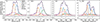 |
Fig. 8. Observations and models of emission lines integrated on the whole system, with residuals shown below each panel. The line doublets ([S II] and [N II]) are displayed as a function of wavelength, and the single lines as a function of LOS velocity. |
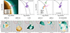 |
Fig. 9. BPT diagrams. Top row, from left to right: [N II] BPT for the five individual components, [N II] BPT for all the components together, [S II] BPT for the five individual components, [S II] BPT for all the components together. Bottom row: Maps with each pixel colour-coded according to the location on the BPT [N II] diagram shown in the top-left panel. Ellipses (or single dot for a2, bis) show the locations of the different components, with the same colour code as in Fig. 7. |
5. Discussion
Figure 10 displays the geometrical configuration of the stellar (left) and gas (right) modelling. We identify four rotating discs that are not yet completely disrupted in the projected field of view of MaNGA (35 kpc in diameter). The maximum difference of the systemic velocity is Δvgas = 600 km/s for the gas and Δvstar = 505 km/s for the stars. We study ram-pressure effects in Sect. 5.1 and possible tidal effects in Sect. 5.2.
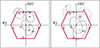 |
Fig. 10. Geometrical configuration. The ellipses in the left (right) panel correspond to the stellar (gas) component of each galaxy, namely its position angle and inclination. The four black bullets correspond to the position of the four galaxies on the sky. The dashed lines correspond to the exponential profiles. The bullets and crosses have the same meanings as in Fig. 2. |
5.1. Ram-pressure stripping
We first estimated the gravitational restoring force per unit mass Pd exerted on the gas content due to the gravitational potential of the galaxy, assuming that gas and stars have the same exponential-disc radial distribution:
 (10)
(10)
where fgas is the gas fraction with respect to the total (stars + gas) disc mass Md, Σ0 = Md/(2πrd2) is the central surface density of the disc, rd is the scale length of the exponential profile, and r the distance from the galactic centre. We assumed that the gas fraction is in the range 5−20%.
Second, given the mass of the cluster A2142 and the projected distance of the galaxy group with respect to the cluster centre (Rgg = 1.3 Mpc), we estimated the cluster density (ρ) at the position of the galaxy group as follows. We considered a Navarro-Frenk-White (NFW) density profile (Navarro et al. 1997), namely
![Mathematical equation: $$ \begin{aligned} \rho _{\mathrm{NFW} }(r) = \rho _0 \, (r/r_0)^{-1} \left[1 + (r/r_0)\right]^{-2}, \end{aligned} $$](/articles/aa/full_html/2026/02/aa56357-25/aa56357-25-eq11.gif) (11)
(11)
with r0 = R200/c. We followed standard conventions: M200 = (4π/3) Δ200 ρc R2003, Δ200 = 200, and ρc = 2.78 × 10¹¹ h2 M⊙ Mpc−3. As summarised in Table 1, we considered M200 = 1.25 × 10¹⁵ M⊙, R200 = 2.16 Mpc, r0 = 0.54 Mpc, and c = 4 (Munari et al. 2014). We then calculated
![Mathematical equation: $$ \begin{aligned} \rho _0 = \Delta _{200} \, \rho _c \, c^3 \times 3^{-1} \times \left[\ln (1 + c) - c(1 + c)^{-1}\right]^{-1} \end{aligned} $$](/articles/aa/full_html/2026/02/aa56357-25/aa56357-25-eq12.gif) (12)
(12)
and estimated ρ0 ≃ 7.18 × 10¹⁴ M⊙ Mpc−3. At r = Rgg, the projected distance of the galaxy group with respect to the cluster centre, it is reasonable to assume that the hot gas profile traces the dark matter NFW profile (e.g. Komatsu & Seljak 2001; Rasia et al. 2004), and therefore ρgas(Rgg)∼fb ρNFW(Rgg)≃3.29 × 10¹² M⊙ Mpc−3, where fb = 0.15 (Planck Collaboration XIII 2016; Tchernin et al. 2016) is the (universal) baryonic fraction. Note that if the group is located at 1.5 Mpc (e.g. Tchernin et al. 2016), this density would be about 30% smaller.
As discussed by Eckert et al. (2014), this galaxy group exhibits a spectacular 700 kpc long X-ray tail that has lasted more than 600 Myr. We could hence estimate the velocity of group in the plane of the sky ( km s−1). In parallel, the radial (or peculiar) velocity could be estimated with the redshift as in Eq. (6).
We hence estimate for the group redshift z = 0.0935, a relative velocity with respect to the cluster of 1126 km s−1, and derive in the frame of the A2142 cluster the following (stellar) radial velocities:  , 1246, 1607 and 1320 km s−1 for the a1, a2, b, and c galaxies. We thus expect the following total velocities for each member of galaxy group (falling inside the MaNGA field of view): Va1tot < 1530 km s−1, Va2tot < 1690 km s−1,
  km s−1, and
  km s−1.
Following Gunn & Gott (1972), we compared the ram pressure (ρgasVgal2) to the force per unit mass (Pdisc) exerted on the gas of disc-galaxies. We hence estimated the radius (rrps) at which all the cold gas of the galaxy disc is stripped using the semi-analytic approximation from Cora et al. (2018):
![Mathematical equation: $$ \begin{aligned} r_{\mathrm{rps} } = -\tfrac{1}{2} \, r_d \, \ln \left[\rho _{\mathrm{gas} } \left(V_{\mathrm{gal} }^{\mathrm{tot} }\right)^2 \left(2 \pi G \, f_{\mathrm{gal} }^{\mathrm{gas} } \, \Sigma _0^2\right)^{-1}\right]. \end{aligned} $$](/articles/aa/full_html/2026/02/aa56357-25/aa56357-25-eq17.gif) (13)
(13)
The disc scale-length is taken from Reff = r1/2 = 1.68rd, and Σ0 from the masses displayed in Table 2. The density of the cluster hot gas ρgas is taken from the previous considerations of the dark matter profile and from X-ray data (Eckert et al. 2014, 2017). The cold gas stripping radius is plotted in Fig. 11 plots. We also took into account the fact that the gas stripping is maximum for a face-on inclination, and minimum for edge-on, as shown by Singh et al. (2024), and have estimated φgal, the angle between the velocity vector and the spin vector for each galaxy.
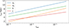 |
Fig. 11. RPS radius as a function of the gas fraction of the galaxy discs. The coloured lines display the values for the disc modelling based on the stellar-derived properties. |
Relying on the direction of the X-ray tail, we estimate its position angle α = 34° with respect to the north direction. In the referential (DEC, RA, LOS), we thus get the following coordinates for the velocity vector V(−Vsky cos α, −Vsky sin α, −Vlos). Vsky is the global velocity modulus of the galaxies in the plane of the sky, assumed to be co-linear with the direction of the X-ray tail. Figure C.2 displays schematically a 3D-rendering of the geometrical distribution of the group positions and velocities. For the unit spin vector of a galaxy (position angle, i), with the usual convention we get sgal(−sin i cos α, −sin i sin α, −cos i). We thus derived the φgal angle between these two vectors as follows:
 (14)
(14)
We thus get φgal = 57°, 56°, 57°, and 53° for a1, a2, b, and c, respectively, which introduces an uncertainty of about 1 kpc on the rrps radius.
Regarding the gas content, we know that the galaxy group is actively forming stars with a global SFR of 42 M⊙ yr−1. Assuming the gas in a region with a typical radius of 5 kpc with a standard depletion time (∼2 Gyr), one expects ΣSFR = 0.5 M⊙ yr−1 kpc−2. Following the typical ‘Kennicutt-Schmidt’ scaling relation (e.g. Fig. 3 in Genzel et al. 2010), one can expect a molecular surface density of Σmol = 530 M⊙ pc−2. Assuming the gas concentrated within a radius of 5 kpc, one can expect a total gas mass of 4.2 × 10¹⁰ fff M⊙, where fff is the filling factor, which could be as low as 1%.
In comparison, the expected mass of the hot gas in the field of view (from the cluster) in a sphere of radius 13.5 kpc is 4 × 10⁷ M⊙. Similarly, one can estimate the mass of the cluster hot gas in the tail, supposed to be shaped as a cone (with 700 kpc length and 150 kpc half-width) is 1011 M⊙.
5.2. Tidal effects
The group of galaxies falling into the Abell 2142 cluster is quite compact, and its galaxies appear in obvious interactions. The group contains four galaxies, two are merging (a1 and a2), and in the others tidal perturbations are detected as tidal tails and loops. In order to provide an estimation of the degree of interaction, based on the total estimated masses, 2D projected distances and relative radial velocities, we calculated the tidal strength affecting the various galaxies.
The total tidal strength produced by a neighbour on each galaxy, with a diameter dg and a mass Mg, is the sum of the tidal forces per unit mass, proportional to Midg/Dig3, where Mi is the mass of the neighbour and Dig is its distance from the centre of the considered galaxy. We approximated Dig via the projected separation at the distance of the galaxy (g). For each galaxy, we summed the tidal forces exerted by its three neighbouring galaxies. We could then compare the total tidal force to the binding force of the galaxy g, i.e. proportional to Mg/dg2. The ratio of tidal to binding forces for each couple of galaxies is Qig = Mi/Mg(dg/Dig)3. The total interaction strength affecting a galaxy g is the sum Qg = ΣiQig. This quantity has been estimated in Table 6.
Tidal strengths estimated using Qig and their sums (Qg).
The most isolated galaxies identified in the sky have their ratio Q of about 10−4, meaning that their total external forces amount only to 0.01% of their internal forces (Verley et al. 2007), while Hickson compact groups have Q between 0.1 and 30. It results from this calculation that the group is highly interacting, with strength comparable to the most compact of galaxy groups (Hickson et al. 1992).
6. Conclusion
We have studied the physical and dynamical state of the galaxy group falling into the galaxy cluster Abell 2142 in order to better quantify the feedback effects of the cluster environment on galaxies. A large fraction of galaxy cluster growth is through such group accretion. This peculiar case is remarkable for the very long (700 kpc) ram pressure tail detected clearly in X-rays. The photometry of the system was made in the ugr bands with ∼1 arcsec (1.7 kpc at z = 0.0935) resolution with MegaCam on the CFHT, and integral field spectroscopy from MaNGA was used to derive stellar and gas kinematics, with 2.6 arcsec (4.5 kpc) and 150−250 km/s resolution depending on wavelength. The full spectral energy distribution was used to derive the age and metallicity of the stellar populations via the NBURSTS package. The gas kinematics and excitation were derived from the line emission of Hα, [N II], [O III], and Hβ. The main difficulty was separating the various components, which correspond to the different galaxies superposed on the LOS. Given that only two spatial coordinates and one radial velocity can be observed, the problem is not well determined, and the solution cannot be unique. For the sake of simplicity, we used parametric models of the four galaxies, with circular velocity and a variable dispersion, combined with simple mass models. We propose a solution compatible with the observations, within the error bars, with the four galaxy rotations disentangled. The kinematics was determined for both stars and gas. Our models are discs dominated by rotation; however, some regions show elevated dispersion, tracing the tidal perturbations. The additional a2, bis component can be interpreted either as the nuclear activity of the central galaxy already confirmed through previous X-ray studies or as the intra-group gas along with the un-modelled residues.
This compact galaxy group lies 1.3 Mpc from the cluster centre, where tidal and ram-pressure effects are difficult to disentangle, and two members are already merging. The four galaxies still host abundant gas and ongoing star formation (∼42 M⊙/yr after AGN correction), indicating that the RPS of their discs is not yet severe. Thus, the long X-ray tail is best explained as the stripping of the group’s hot intra-group medium during its infall into Abell 2142, rather than as the direct stripping of the galaxies themselves.
Acknowledgments
We thank the anonymous referee for their comments and suggestions. DG’s research on the NBURSTS fitting of the spectrum, and interpretation of the kinematic and properties of stellar population was supported by the Russian Science Foundation (RSCF) grants No. 23-12-00146. This work was also supported by the Programme National Cosmologie et Galaxies (PNCG) of CNRS/INSU with INP and IN2P3, 883 co-funded by CEA and CNES.
References
- Alam, S., Albareti, F. D., Allende Prieto, C., et al. 2015, ApJS, 219, 12 [Google Scholar]
- Bahcall, N. A. 1977, ARA&A, 15, 505 [Google Scholar]
- Baldwin, J. A., Phillips, M. M., & Terlevich, R. 1981, PASP, 93, 5 [Google Scholar]
- Bekki, K. 1999, ApJ, 510, L15 [NASA ADS] [CrossRef] [Google Scholar]
- Bekki, K. 2009, MNRAS, 399, 2221 [Google Scholar]
- Benavides, J. A., Sales, L. V., & Abadi, M. G. 2020, MNRAS, 498, 3852 [Google Scholar]
- Bianconi, M., Smith, G. P., Haines, C. P., et al. 2018, MNRAS, 473, L79 [CrossRef] [Google Scholar]
- Bilton, L. E., & Pimbblet, K. A. 2018, MNRAS, 481, 1507 [CrossRef] [Google Scholar]
- Boselli, A., & Gavazzi, G. 2006, PASP, 118, 517 [Google Scholar]
- Boselli, A., Fossati, M., & Sun, M. 2022, A&ARv, 30, 3 [NASA ADS] [CrossRef] [Google Scholar]
- Bower, R. G., & Balogh, M. L. 2004, in Clusters of Galaxies: Probes of Cosmological Structure and Galaxy Evolution, eds. J. S. Mulchaey, A. Dressler, & A. Oemler, 325 [Google Scholar]
- Bruno, L., Botteon, A., Shimwell, T., et al. 2023, A&A, 678, A133 [NASA ADS] [CrossRef] [EDP Sciences] [Google Scholar]
- Bundy, K., Bershady, M. A., Law, D. R., et al. 2015, ApJ, 798, 7 [Google Scholar]
- Buote, D. A., & Tsai, J. C. 1996, ApJ, 458, 27 [NASA ADS] [CrossRef] [Google Scholar]
- Bykov, A. M., Kaastra, J. S., Brüggen, M., et al. 2019, Space Sci. Rev., 215, 27 [NASA ADS] [CrossRef] [Google Scholar]
- Calzetti, D., Armus, L., Bohlin, R. C., et al. 2000, ApJ, 533, 682 [NASA ADS] [CrossRef] [Google Scholar]
- Chilingarian, I., Prugniel, P., Sil’Chenko, O., & Koleva, M. 2007a, IAU Symp., 241, 175 [Google Scholar]
- Chilingarian, I. V., Prugniel, P., Sil’Chenko, O. K., & Afanasiev, V. L. 2007b, MNRAS, 376, 1033 [NASA ADS] [CrossRef] [Google Scholar]
- Choque-Challapa, N., Smith, R., Candlish, G., Peletier, R., & Shin, J. 2019, MNRAS, 490, 3654 [NASA ADS] [CrossRef] [Google Scholar]
- Chung, A., van Gorkom, J. H., Kenney, J. D. P., & Vollmer, B. 2007, ApJ, 659, L115 [Google Scholar]
- Comerford, J. M., Nevin, R., Negus, J., et al. 2024, ApJ, 963, 53 [NASA ADS] [CrossRef] [Google Scholar]
- Cora, S. A., Vega-Martínez, C. A., Hough, T., et al. 2018, MNRAS, 479, 2 [Google Scholar]
- Drory, N., MacDonald, N., Bershady, M. A., et al. 2015, AJ, 149, 77 [CrossRef] [Google Scholar]
- Eckert, D., Molendi, S., Owers, M., et al. 2014, A&A, 570, A119 [NASA ADS] [CrossRef] [EDP Sciences] [Google Scholar]
- Eckert, D., Gaspari, M., Owers, M. S., et al. 2017, A&A, 605, A25 [NASA ADS] [CrossRef] [EDP Sciences] [Google Scholar]
- Einasto, M., Gramann, M., Saar, E., et al. 2015, A&A, 580, A69 [NASA ADS] [CrossRef] [EDP Sciences] [Google Scholar]
- Einasto, M., Deshev, B., Lietzen, H., et al. 2018, A&A, 610, A82 [NASA ADS] [CrossRef] [EDP Sciences] [Google Scholar]
- Einasto, M., Deshev, B., Tenjes, P., et al. 2020, A&A, 641, A172 [NASA ADS] [CrossRef] [EDP Sciences] [Google Scholar]
- Fillingham, S. P., Cooper, M. C., Pace, A. B., et al. 2016, MNRAS, 463, 1916 [Google Scholar]
- Gasymov, D., & Katkov, I. 2024, ASP Conf. Ser., 535, 279 [Google Scholar]
- Genzel, R., Tacconi, L. J., Gracia-Carpio, J., et al. 2010, MNRAS, 407, 2091 [NASA ADS] [CrossRef] [Google Scholar]
- Gunn, J. E., & Gott, J. R. 1972, ApJ, 176, 1 [NASA ADS] [CrossRef] [Google Scholar]
- Gwyn, S. D. J. 2008, PASP, 120, 212 [Google Scholar]
- Hausammann, L., Revaz, Y., & Jablonka, P. 2019, A&A, 624, A11 [NASA ADS] [CrossRef] [EDP Sciences] [Google Scholar]
- Hickson, P., Mendes de Oliveira, C., Huchra, J. P., & Palumbo, G. G. 1992, ApJ, 399, 353 [Google Scholar]
- Hubble, E. P. 1926, ApJ, 64, 321 [Google Scholar]
- Jáchym, P., Kenney, J. D. P., Ržuička, A., et al. 2013, A&A, 556, A99 [NASA ADS] [CrossRef] [EDP Sciences] [Google Scholar]
- Jáchym, P., Combes, F., Cortese, L., Sun, M., & Kenney, J. D. P. 2014, ApJ, 792, 11 [Google Scholar]
- Jáchym, P., Sun, M., Kenney, J. D. P., et al. 2017, ApJ, 839, 114 [Google Scholar]
- Jin, G., Dai, Y. S., Pan, H.-A., et al. 2021, ApJ, 923, 6 [NASA ADS] [CrossRef] [Google Scholar]
- Kasparova, A. V., Katkov, I. Y., & Chilingarian, I. V. 2020, MNRAS, 493, 5464 [NASA ADS] [CrossRef] [Google Scholar]
- Katkov, I. Y., Sil’chenko, O. K., & Afanasiev, V. L. 2013, ApJ, 769, 105 [NASA ADS] [CrossRef] [Google Scholar]
- Katkov, I. Y., Sil’chenko, O. K., Chilingarian, I. V., Uklein, R. I., & Egorov, O. V. 2016, MNRAS, 461, 2068 [Google Scholar]
- Katkov, I. Y., Gasymov, D., Kniazev, A. Y., et al. 2024, ApJ, 962, 27 [NASA ADS] [CrossRef] [Google Scholar]
- Kennicutt, R. C. 1998, ARA&A, 36, 189 [NASA ADS] [CrossRef] [Google Scholar]
- Kleiner, D., Serra, P., Maccagni, F. M., et al. 2021, A&A, 648, A32 [NASA ADS] [CrossRef] [EDP Sciences] [Google Scholar]
- Komatsu, E., & Seljak, U. 2001, MNRAS, 327, 1353 [Google Scholar]
- Kuchner, U., Haggar, R., Aragón-Salamanca, A., et al. 2022, MNRAS, 510, 581 [Google Scholar]
- Li, C., Kauffmann, G., Heckman, T. M., Jing, Y. P., & White, S. D. M. 2008, MNRAS, 385, 1903 [NASA ADS] [CrossRef] [Google Scholar]
- Liu, A., Yu, H., Diaferio, A., et al. 2018, ApJ, 863, 102 [NASA ADS] [CrossRef] [Google Scholar]
- Lopes, P. A. A., Ribeiro, A. L. B., & Brambila, D. 2024, MNRAS, 527, L19 [Google Scholar]
- Lupton, R., Blanton, M. R., Fekete, G., et al. 2004, PASP, 116, 133 [NASA ADS] [CrossRef] [Google Scholar]
- Markevitch, M., Ponman, T. J., Nulsen, P. E. J., et al. 2000, ApJ, 541, 542 [Google Scholar]
- Marshall, M. A., Shabala, S. S., Krause, M. G. H., et al. 2018, MNRAS, 474, 3615 [NASA ADS] [CrossRef] [Google Scholar]
- Mateus, A., Sodré, L., Cid Fernandes, R., & Stasińska, G. 2007, MNRAS, 374, 1457 [NASA ADS] [CrossRef] [Google Scholar]
- Munari, E., Biviano, A., & Mamon, G. A. 2014, A&A, 566, A68 [NASA ADS] [CrossRef] [EDP Sciences] [Google Scholar]
- Munari, E., Grillo, C., De Lucia, G., et al. 2016, ApJ, 827, L5 [Google Scholar]
- Navarro, J. F., Frenk, C. S., & White, S. D. M. 1997, ApJ, 490, 493 [Google Scholar]
- Okabe, N., & Umetsu, K. 2008, PASJ, 60, 345 [NASA ADS] [Google Scholar]
- Osterbrock, D. E., & Ferland, G. J. 2006, Astrophysics of Gaseous Nebulae and Active Galactic Nuclei (Sausalito: University Science Books) [Google Scholar]
- Pasquali, A. 2015, Astron. Nachr., 336, 505 [NASA ADS] [CrossRef] [Google Scholar]
- Peluso, G., Vulcani, B., Poggianti, B. M., et al. 2022, ApJ, 927, 130 [NASA ADS] [CrossRef] [Google Scholar]
- Peng, C. Y., Ho, L. C., Impey, C. D., & Rix, H.-W. 2002, AJ, 124, 266 [Google Scholar]
- Peng, C. Y., Ho, L. C., Impey, C. D., & Rix, H.-W. 2010, AJ, 139, 2097 [Google Scholar]
- Planck Collaboration XIII. 2016, A&A, 594, A13 [NASA ADS] [CrossRef] [EDP Sciences] [Google Scholar]
- Planck Collaboration XXVII. 2016, A&A, 594, A27 [NASA ADS] [CrossRef] [EDP Sciences] [Google Scholar]
- Poggianti, B. M., Jaffé, Y. L., Moretti, A., et al. 2017, Nature, 548, 304 [Google Scholar]
- Poopakun, K., & Kriwattanawong, W. 2019, J. Phys. Conf. Ser., 1380, 012064 [Google Scholar]
- Pranger, F., Trujillo, I., Kelvin, L. S., & Cebrián, M. 2017, MNRAS, 467, 2127 [NASA ADS] [CrossRef] [Google Scholar]
- Rasia, E., Tormen, G., & Moscardini, L. 2004, MNRAS, 351, 237 [NASA ADS] [CrossRef] [Google Scholar]
- Ricarte, A., Tremmel, M., Natarajan, P., & Quinn, T. 2020, ApJ, 895, L8 [NASA ADS] [CrossRef] [Google Scholar]
- Salim, S., Lee, J. C., Janowiecki, S., et al. 2016, ApJS, 227, 2 [NASA ADS] [CrossRef] [Google Scholar]
- Sanders, D. B., Soifer, B. T., Elias, J. H., et al. 1988, ApJ, 325, 74 [Google Scholar]
- Scott, T. C., Cortese, L., Brinks, E., et al. 2012, MNRAS, 419, L19 [Google Scholar]
- Singh, A., Davessar, S., Gulati, M., Bagla, J. S., & Prajapati, M. 2024, MNRAS, 530, 699 [Google Scholar]
- Springel, V., Frenk, C. S., & White, S. D. M. 2006, Nature, 440, 1137 [NASA ADS] [CrossRef] [Google Scholar]
- Steinhauser, D., Schindler, S., & Springel, V. 2016, A&A, 591, A51 [NASA ADS] [CrossRef] [EDP Sciences] [Google Scholar]
- Sun, M., Jones, C., Forman, W., et al. 2006, ApJ, 637, L81 [Google Scholar]
- Tchernin, C., Eckert, D., Ettori, S., et al. 2016, A&A, 595, A42 [NASA ADS] [CrossRef] [EDP Sciences] [Google Scholar]
- Vazdekis, A., Koleva, M., Ricciardelli, E., Röck, B., & Falcón-Barroso, J. 2016, MNRAS, 463, 3409 [Google Scholar]
- Verley, S., Leon, S., Verdes-Montenegro, L., et al. 2007, A&A, 472, 121 [NASA ADS] [CrossRef] [EDP Sciences] [Google Scholar]
- Vijayaraghavan, R., & Ricker, P. M. 2013, MNRAS, 435, 2713 [NASA ADS] [CrossRef] [Google Scholar]
- Vikhlinin, A. A., Kravtsov, A. V., Markevich, M. L., Sunyaev, R. A., & Churazov, E. M. 2014, Phys. Usp., 57, 317 [NASA ADS] [CrossRef] [Google Scholar]
- Vulcani, B., Poggianti, B. M., Gullieuszik, M., et al. 2018, ApJ, 866, L25 [Google Scholar]
- Westfall, K. B., Cappellari, M., Bershady, M. A., et al. 2019, AJ, 158, 231 [Google Scholar]
For galaxies b and c, this differs from the stellar fit for which the discs are centred on the centres of the ‘extended’ components. However, for galaxy b, emission line fluxes are the largest in the MaNGA pixel containing the centre of the core component, making it logical to place the centre of the simulated disc there, and we similarly used the centre of the core component for galaxy c, which is too close to the edges of the field of view to check fluxes near the centre of the extended component.
Appendix A: Subaru images
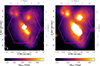 |
Fig. A.1. Subaru g-band (left) and r-band (right) images, from the JVO Subaru Suprime-Cam mosaic image archive. Available here for g and here. |
Appendix B: Stellar analysis
 |
Fig. B.1. Example of two-component NBURSTS fitting for the region with a1 and b galaxies. The black line shows the observed spectrum in the spaxel, and blue is the total best-fitting model. Red and green lines are stellar components of a1 and b galaxies, and the orange line is the emission line component. Black dots are residuals, and the grey line shows the spectrum errors. The shaded regions were excluded from fitting, and the purple line is the multiplicative continuum. The growing trend from the blue to the red spectrum part of the multiplicative continuum is a correction for the extinction. |
 |
Fig. B.2. Non-parametric recovery of the stellar LOSVD. We show the recovered LOSVD derived from the spectral binning in each spaxel of the MaNGA spectrum using Gaussian fitting techniques. The number of Gaussian components fitted varies according to the spatial location of each spaxel. Initially, all spaxels were fitted with a Gaussian representing the a1 component (in blue). Additional Gaussian components were incorporated in regions where extra kinematic structures were identified (denoted by circles a2, b, and c, and coded in orange, green, and red). The merged spaxels used for the two-component full-spectrum fitting are shown as highlighted regions in the corresponding colours. Within these regions, vertical lines mark the velocities obtained from the full-spectrum fitting procedure, which are consistent with the two-Gaussian fits of the recovered non-parametric LOSVDs. |
Appendix C: Gas analysis
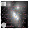 |
Fig. C.1. [O III]5008 Angstroms MaNGA observations and models of four galaxies and a broad component (a2, bis), superimposed on the MegaCam r-band image. MaNGA pixels encompassing the centre of each modelled component are shown. Fits were done on original MaNGA spaxels, but for the figure MaNGA spectra and our fits are binned 16 by 16 and shown in brown boxes encompassing these binned spaxels. The velocity axis of each box is from -1000 to 1000 km/s. The two same ticks for values 0, on the baseline of spectra, and 0.01 are shown on the left and right y axes of each box to show the scale that is adapted to each box. The Gaussian reconstructed MaNGA PSF is shown on the bottom left. The MaNGA hexagonal field of view is represented in black. |
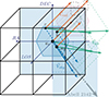 |
Fig. C.2. Kinematical configuration. The four black bullets correspond to the position of the four galaxies on the sky. 3D velocities, labelled Vtot and associated with each galaxy, are displayed as green arrows. Velocities in the plane of the sky, as derived from the X-ray tail, are displayed as blue arrows. The radial velocities associated with the redshift of each galaxy are displayed in orange. The filled rectangles lie in the plane of the sky as well as the MaNGA hexagonal field and are displayed in blue. (In order to give an overview of the 3D effect, we added a purple hexagon projected at the main redshift velocity.) The grey arrow (in the plane of the sky) points towards the centre of A2142. |
All Tables
SFR per galaxy from our modelling derived using two extinction laws, with an additional broad component, a2, bis.
All Figures
|
Fig. 1. SDSS (Data Release 12) gri image (left), MegaPipe ugr image (centre), and unsharp masking of the MegaPipe r-band image (right), with the MaNGA field of view overlaid in magenta. The three main stellar regions are segregated and marked as (a, b, c) on the SDSS image. The centres of the regions, with a subdivision of the a region into two galaxies, are shown on the MegaPipe images. |
| In the text | |
|
Fig. 2. Photometric modelling of the CFHT MegaPipe r-band image using GALFIT. Blue hexagons show the MaNGA field of view, ‘x’ symbols indicate the centres of the ‘core’ components, dots near the c and b components indicate the centres of the ‘outskirts’ components, and the dot between a1 and a2 is the centre of the‘bridge’ between them (see Sect. 3.1.2). Dashed ellipses show the effective radius of the most ‘extended’ component of each galaxy, based on the parameters from Table 2. Third panel shows the residuals-to-data ratio. The colour bar unit is proportional to the analogue-to-digital unit. |
| In the text | |
|
Fig. 3. Emission line maps from NBURSTS single Gaussian fits. The main emission lines (Hα, Hβ, [O III]5008, and [N II]6585) are displayed in arbitrary units; the gas velocity dispersions fixed to all lines are in km/s. The x and y coordinates are in MaNGA pixels of 0.4″. |
| In the text | |
|
Fig. 4. Difference between the stellar and gas velocity. |
| In the text | |
|
Fig. 5. Kinematical modelling of the stellar recovered LOSVD. The panels show the velocity maps of the different components and their corresponding models (see Sect. 3.1.2). Blue hexagons show the field of view covered by the MaNGA observations. |
| In the text | |
|
Fig. 6. Superposition of all [O III] lines from each pixel, colour-coded by the position of the pixel (as shown in the left panel). Bottom left: SDSS g-band image (black contours). The hexagon is the field of view of MaNGA. Top: Spectra of the whole map. Middle right: Top half of the field (i.e. the field above the dotted white line in the bottom-left panel), emphasising regions where galaxies b and c are present. Bottom right: Bottom half of the field, highlighting areas where galaxies a1 and a2 are situated. |
| In the text | |
|
Fig. 7. Observations, models, and residuals of the flux, velocity, and velocity dispersion from the [O III]5008 Angstrom line. Models are shown for each component (Cols. 2 to 6) and for the five components together (Col. 7). Residuals (Col. 8) are the observation (Col. 1) minus the model (Col. 7). On the velocity maps of individual galaxies, iso-LOS velocity curves are represented in dashed (solid) black lines for values below (above) the systemic velocity of each galaxy. |
| In the text | |
|
Fig. 8. Observations and models of emission lines integrated on the whole system, with residuals shown below each panel. The line doublets ([S II] and [N II]) are displayed as a function of wavelength, and the single lines as a function of LOS velocity. |
| In the text | |
|
Fig. 9. BPT diagrams. Top row, from left to right: [N II] BPT for the five individual components, [N II] BPT for all the components together, [S II] BPT for the five individual components, [S II] BPT for all the components together. Bottom row: Maps with each pixel colour-coded according to the location on the BPT [N II] diagram shown in the top-left panel. Ellipses (or single dot for a2, bis) show the locations of the different components, with the same colour code as in Fig. 7. |
| In the text | |
|
Fig. 10. Geometrical configuration. The ellipses in the left (right) panel correspond to the stellar (gas) component of each galaxy, namely its position angle and inclination. The four black bullets correspond to the position of the four galaxies on the sky. The dashed lines correspond to the exponential profiles. The bullets and crosses have the same meanings as in Fig. 2. |
| In the text | |
|
Fig. 11. RPS radius as a function of the gas fraction of the galaxy discs. The coloured lines display the values for the disc modelling based on the stellar-derived properties. |
| In the text | |
|
Fig. A.1. Subaru g-band (left) and r-band (right) images, from the JVO Subaru Suprime-Cam mosaic image archive. Available here for g and here. |
| In the text | |
|
Fig. B.1. Example of two-component NBURSTS fitting for the region with a1 and b galaxies. The black line shows the observed spectrum in the spaxel, and blue is the total best-fitting model. Red and green lines are stellar components of a1 and b galaxies, and the orange line is the emission line component. Black dots are residuals, and the grey line shows the spectrum errors. The shaded regions were excluded from fitting, and the purple line is the multiplicative continuum. The growing trend from the blue to the red spectrum part of the multiplicative continuum is a correction for the extinction. |
| In the text | |
|
Fig. B.2. Non-parametric recovery of the stellar LOSVD. We show the recovered LOSVD derived from the spectral binning in each spaxel of the MaNGA spectrum using Gaussian fitting techniques. The number of Gaussian components fitted varies according to the spatial location of each spaxel. Initially, all spaxels were fitted with a Gaussian representing the a1 component (in blue). Additional Gaussian components were incorporated in regions where extra kinematic structures were identified (denoted by circles a2, b, and c, and coded in orange, green, and red). The merged spaxels used for the two-component full-spectrum fitting are shown as highlighted regions in the corresponding colours. Within these regions, vertical lines mark the velocities obtained from the full-spectrum fitting procedure, which are consistent with the two-Gaussian fits of the recovered non-parametric LOSVDs. |
| In the text | |
|
Fig. C.1. [O III]5008 Angstroms MaNGA observations and models of four galaxies and a broad component (a2, bis), superimposed on the MegaCam r-band image. MaNGA pixels encompassing the centre of each modelled component are shown. Fits were done on original MaNGA spaxels, but for the figure MaNGA spectra and our fits are binned 16 by 16 and shown in brown boxes encompassing these binned spaxels. The velocity axis of each box is from -1000 to 1000 km/s. The two same ticks for values 0, on the baseline of spectra, and 0.01 are shown on the left and right y axes of each box to show the scale that is adapted to each box. The Gaussian reconstructed MaNGA PSF is shown on the bottom left. The MaNGA hexagonal field of view is represented in black. |
| In the text | |
|
Fig. C.2. Kinematical configuration. The four black bullets correspond to the position of the four galaxies on the sky. 3D velocities, labelled Vtot and associated with each galaxy, are displayed as green arrows. Velocities in the plane of the sky, as derived from the X-ray tail, are displayed as blue arrows. The radial velocities associated with the redshift of each galaxy are displayed in orange. The filled rectangles lie in the plane of the sky as well as the MaNGA hexagonal field and are displayed in blue. (In order to give an overview of the 3D effect, we added a purple hexagon projected at the main redshift velocity.) The grey arrow (in the plane of the sky) points towards the centre of A2142. |
| In the text | |
Current usage metrics show cumulative count of Article Views (full-text article views including HTML views, PDF and ePub downloads, according to the available data) and Abstracts Views on Vision4Press platform.
Data correspond to usage on the plateform after 2015. The current usage metrics is available 48-96 hours after online publication and is updated daily on week days.
Initial download of the metrics may take a while.