| Issue |
A&A
Volume 706, February 2026
|
|
|---|---|---|
| Article Number | A7 | |
| Number of page(s) | 16 | |
| Section | Interstellar and circumstellar matter | |
| DOI | https://doi.org/10.1051/0004-6361/202556926 | |
| Published online | 28 January 2026 | |
Weak, extended water vapor emission in the Horsehead nebula
1
Jet Propulsion Laboratory, California Institute of Technology,
4800 Oak Drove Drive,
Pasadena,
CA
91109,
USA
2
LUX, Observatoire de Paris, Université PSL, CNRS, Sorbonne Université,
92190
Meudon,
France
3
Instituto de Física Fundamental (CSIC),
Calle Serrano 121–123,
28006
Madrid,
Spain
4
European Space Agency (ESA), European Space Astronomy Centre (ESAC), Camino bajo del Castillo, s/n, Urbanización Villafranca del Castillo, Villanueva de la Cañada,
28692
Madrid,
Spain
★ Corresponding author: This email address is being protected from spambots. You need JavaScript enabled to view it.
Received:
20
August
2025
Accepted:
1
December
2025
Abstract
We analyzed archival Herschel observations of water vapor emission toward the Horsehead photon dominated region (PDR) along with supporting ground-based and airborne observations of CO isotopologs and fine structure lines of ionized and atomic carbon to determine the distribution and abundance of water vapor in this low-UV illumination PDR. Water emission in the Horsehead nebula is very weak and, surprisingly, extends outward beyond other PDR tracers such as 12CO or [C I] 609 μm, reaching as far out as [C II] 158 μm. We modeled the observations using a newly developed PDR wrapper that takes into account the geometry of this region. The PDR modeling of the molecular and atomic lines studied here provides strong constraints on the thermal pressure, but not on the UV illumination. Maximum model line intensities and spatial profiles are well reproduced, except for CO isotopologs, where the increase on the illuminated side of the PDR is steeper than observed. Water vapor abundance in the model reaches 3.6 × 10⁻⁷ at AV ~ 3 mag. However, the ground state o-H2O 557 GHz line is systematically overestimated by the models by at least a factor of seven for any values of the model parameters. This line has a very high optical depth and the emergent line intensity is sensitive to radiative transfer effects such as line scattering by water molecules in a low-density halo surrounding the dense PDR and the assumed microturbulent line width. A more accurate model of the water surface chemistry is required.
Key words: stars: formation / ISM: abundances / ISM: atoms / ISM: molecules / photon-dominated region (PDR) / ISM: individual objects: Horsehead nebula
© The Authors 2026
 Open Access article, published by EDP Sciences, under the terms of the Creative Commons Attribution License (https://creativecommons.org/licenses/by/4.0), which permits unrestricted use, distribution, and reproduction in any medium, provided the original work is properly cited.
This article is published in open access under the Subscribe to Open model. This email address is being protected from spambots. You need JavaScript enabled to view it. to support open access publication.
1 Introduction
Understanding how the Earth obtained its water and whether water-rich earthlike planets are common in the Universe is a fundamental cosmic origins question. Water forms efficiently in the cold interstellar medium via low-temperature ion-neutral chemistry or grain surface chemistry (van Dishoeck et al. 2013). Gaseous water and water-ice covered dust grains, either pristine or partially reprocessed, make their way through the subsequent stages of star formation, including dense cores and protostellar disks, before being incorporated into planetesimals in forming planetary systems (van Dishoeck et al. 2021). Understanding whether water and organics available for delivery to nascent planets in habitable zones around stars are supplied from their initial interstellar reservoir through a process that operates universally in forming planetary systems is a subject of active research. The possible links between the composition of interstellar and Solar System materials are of great interest for understanding the Solar System beginnings (Bockelée-Morvan et al. 2000; Drozdovskaya et al. 2019).
An investigation of the “water trail” was one of the main science themes of the Herschel Space Observatory (van Dishoeck et al. 2021). Herschel observations demonstrated that gas-phase water abundance is universally low, often orders of magnitude below the canonical value of 4 × 10⁻⁴ with respect to the molecular hydrogen, expected if all volatile oxygen is locked in water. Water vapor emission in molecular clouds was also found to be weak and difficult to detect away from embedded protostars. Melnick et al. (2011, 2020) concluded that water vapor is confined primarily within a few magnitudes of dense cloud surfaces. An exception are photon dominated regions (PDRs), surface layers of molecular clouds exposed to enhanced UV radiation.
Putaud et al. (2019) analyzed velocity-resolved observations of multiple water lines in the Orion Bar, one of the best studied PDRs, where warm chemistry with water ice desorption dominates. Using the Meudon PDR code (Le Petit et al. 2006), they derived the water abundance and ortho-para ratio in this region. They concluded that gas-phase water arises from a region deep into the cloud, corresponding to a visual extinction of AV ~ 9. The ![Mathematical equation: $\[\mathrm{H}_2^{16} \mathrm{O}\]$](/articles/aa/full_html/2026/02/aa56926-25/aa56926-25-eq1.png) fractional abundance in this region is ~2 × 10⁻⁷, and the total water column density is (1.4 ± 0.8) × 1015 cm−2. Contrary to earlier suggestions, a line-of-sight averaged ortho-para ratio was found to be consistent with a nuclear spin isomer repartition at the temperature of the water-emitting gas, 36 ± 2 K.
fractional abundance in this region is ~2 × 10⁻⁷, and the total water column density is (1.4 ± 0.8) × 1015 cm−2. Contrary to earlier suggestions, a line-of-sight averaged ortho-para ratio was found to be consistent with a nuclear spin isomer repartition at the temperature of the water-emitting gas, 36 ± 2 K.
Pilleri et al. (2012) analyzed observations of water vapor in Mon R2, where the associated strongly irradiated PDR could be spatially resolved with Herschel. They derived a low mean abundance of o-H2O of ~10−8 relative to H2, and a higher abundance of ~10−7 in the high-velocity wings detected toward the H II region.
The Orion Bar is a dense PDR characterized by a very high flux of UV photons with Go = (3–5) × 104 in Habing units (Peeters et al. 2024) and a high thermal pressure of ~(1–3) × 108 K cm−3 (Joblin et al. 2018; Putaud et al. 2019). Mon R2 is a relatively distant (830 pc) high-mass star forming region with a complex morphology and Go = 5 × 10⁵ in its PDR. In the present work we analyze observations of water and other molecular and atomic tracers toward the Horsehead nebula, a region characterized by a simple geometry and much lower UV illumination with G0 ~ 100 (Santa-Maria et al. 2023), which is more representative of the average UV-illuminated neutral gas in the Milky Way (e.g., Cubick et al. 2008). The archival data used in the analysis are described in Section 2, the results are presented in Section 3, and the PDR models used to interpret the observations are discussed in Section 4. Section 6 gives a summary and conclusions.
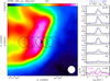 |
Fig. 1 (Left panel) SPIRE 350 μm image of the Horsehead PDR. The white circle shows the FWHM SPIRE beam (25.2″). Black circles show the locations at which 557 GHz o-H2O spectra were obtained, with the circle size corresponding to the FWHM HIFI beam (38.1″). (Right panel) Spectra of the 557 GHz o-H2O and CO (2–1) lines across the PDR (black and blue curves, respectively), labeled by the right ascension offsets with respect to the reference position. The CO 2–1 spectra have been scaled down by a factor of 200. The bottom-right panel shows spectra of the ground state o– and p–H2O lines at the central position. |
2 Archival data
The 557 GHz 110–101 ground-state ortho-water line was observed in the frequency-switched (FSW) mode at six positions along a right ascension strip across the Horsehead PDR using the HIFI instrument (de Graauw et al. 2010) aboard the Herschel Space Observatory (Pilbratt et al. 2010) as a part of the open time program OT_dteyssie_2 (Herschel OBSID 1342203151). Spectra were taken at right ascension offsets from −40 to +60″, with 20" spacing, with respect to the center position αJ2000 = 05h40m53.7s, δJ2000 = −2°28′00″. In addition, FSW spectra of the same ortho-water line and the 1113 GHz 111–000 ground-state para-water line were observed at the center position as a part of guaranteed time program KPGT_vossenko_1 (OBSIDs 1342203191 and 1342217721). The on-source integration time is ~30 min per point for the 557 GHz line and 63 min for the 1113 Ghz line.
In our analysis, we used spectra obtained with the HIFI wide-band spectrometer (WBS) as a backend, which provided 1.1 MHz spectral resolution for H and V instrumental polarizations. The two polarizations were averaged together with equal weighting. The data downloaded from the ESA Herschel Science Archive1 were reduced with version 14.1.0 of the HIFI pipeline. The latest values of the HIFI beam efficiencies of 0.635 at 557 GHz and 0.59 at 1113 GHz were applied to convert the spectra to the main beam brightness temperature scale.
The total observing time for the H2O 110–101 strip varied between 20.2 and 33.1 min per position, resulting in an rms noise level between 3.0 and 4.6 mK in a single spectrometer channel. The integration times for the additional spectra toward the center positions were 27.8 and 63.1 min, for ortho- and para-water lines, respectively. However, these spectra are affected by baseline ripples and have relatively high rms noise levels of 9.3 and 18.8 mK, respectively.
In addition to the HIFI water spectra described above, we used in the analysis ground-based observations of the Horsehead nebula from Philipp et al. (2006), which include ~15″ resolution single-dish images of the [C I] 609 μm and CO (4–3) lines carried out using the CHAMP array at the Caltech Submillimeter Observatory, as well as observations of the (2–1) transitions of the CO isotopologs carried out with the IRAM 30 m telescope. We also used archival observations of [C II] downloaded from the SOFIA Science Archive at IRSA/IPAC2.
3 Results
Figure 1 shows the overall morphology of the Horsehead PDR as traced by the 350 μm dust continuum emission observed with the SPIRE instrument on Herschel. The center position for the HIFI water observations is marked with a black asterisk, and the black circles show locations of the HIFI beams at the six positions along the strip. The white circle shows the full width at half maximum (FWHM) SPIRE beam at 350 μm.
The velocity-resolved HIFI water spectra of the 557 GHz along the east-west strip across the PDR are shown as black histograms in the top six panels on the right. The panels are labeled with the corresponding right ascension offset with respect to the reference position. CO (2–1) spectra from Philipp et al. (2006) at the same position are shown in blue. The water spectra are generally broader than CO spectra, indicating high line opacity. In particular, the water spectrum at the center (Δα = 0) position shows a self-absorption line profile. The bottom-right panel shows the additional spectra of the ortho- and para-water lines at the center position.
Figure 2 shows integrated line intensities of the various atomic and molecular tracers as a function of right ascension offset with respect to the reference position at a zero declination offset. The upper panel shows a clear stratification between the ionized and neutral carbon, with water emission peaking behind both tracers. The lower panels shows the distribution of water emission as compared to the three CO isotopologs. The water emission peaks at a similar location C18O, but extends further out into the ionized region.
To determine whether the observed stratification may be due to the differences in the angular resolution of the data, we convolved all images to the lowest spatial resolution of the HIFI o-H2O data. The resulting strips are shown in Figure 3. The same stratification can still be seen, with water emission extending further out into the ionized region compared to other tracers. Integrated water line intensities between 7 and 14 km s−1 at different positions are listed in Table 1 along with the corresponding uncertainties. Maximum line intensities of the various atomic and molecular tracers considered here in the HIFI beam are listed in Table 2.
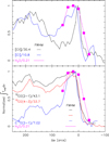 |
Fig. 2 Integrated line intensities of atomic and molecular tracers computed over a 9.2–11.8 km s−1 velocity range across the PDR as a function of right ascension offset at Δδ = 0. (Top) [C II], [C I], and H2O (black, blue, and magenta, respectively). (Bottom) CO (2–1), C18O (2–1), CO (4–3), and H2O (black, blue, red, and magenta, respectively). Line intensities have been normalized to their maxima toward the PDR, with the corresponding scaling factors as labeled. The data are shown at the native resolution of the images, with the corresponding FWHM beam sizes marked for each tracer. The size of the squares corresponds approximately to ±1σ H2O observational uncertainties. |
4 Pseudo 2-D PDR modeling of the Horsehead nebula
4.1 Previous approaches to model the Horsehead geometry with 1D plane-parallel codes
The Horsehead nebula has long served as a benchmark for the study of PDRs, owing to its well-defined, nearly edge-on geometry and wealth of multiwavelength observational data (e.g., Pety et al. 2005). Despite its apparent spatial simplicity, modeling the Horsehead poses specific challenges. Most PDR models, including those using the Meudon PDR code, adopt a 1D plane-parallel slab geometry in which the radiation field and physicochemical gradients vary the depth into the cloud, as the UV photons are gradually attenuated by dust. However, in the case of the Horsehead, the PDR is viewed nearly edge-on, meaning that the observer’s line of sight is perpendicular to the primary gradient direction in the model. As a result, direct comparisons between model predictions (computed along the depth axis) and observational quantities (integrated along the line of sight) require nontrivial adaptations, typically involving assumptions about the effective length of the PDR along the line of sight or geometrical corrections.
Habart et al. (2005), using SOFI observations of the H2 1–0 S(1) line at the NTT, modeled the Horsehead nebula as an edge-on, semi-infinite plane-parallel slab illuminated by an external radiation field and exhibiting a steep density gradient. This structure corresponded to an isobaric PDR with a thermal pressure of 4 × 10⁶ K cm−3. The computed emissivity was then scaled by the PDR length along the line of sight, assumed to be at most equal to the filament’s extent in the plane of the sky, i.e., approximately 0.1 pc.
Goicoechea et al. (2006) first used the output of Meudon PDR models as input for non-local thermodynamic equilibrium (non-LTE) radiative transfer models of CS and C18O emission lines, adapted to the edge-on geometry of the PDR. Similarly, Pabst et al. (2017) used the predictions of a face-on PDR model to calculate the expected [C II] 158 μm line emission. Both approaches compute the line-of-sight radiative transfer assuming 1D plane-parallel slabs.
Guzmán et al. (2011) also employed Meudon PDR models with a steep density gradient to interpret H2CO transition lines observed with the IRAM-30m telescope, which were converted into chemical abundances. These derived abundances were compared to model predictions with and without surface chemistry, at two positions in the cloud referred to as the “core” and the “PDR”. A similar methodology (direct comparison between observed abundances and Meudon PDR model outputs) was applied in the interpretation of IRAM-30m observations of CF+, l-C3H+, CH3OH, and HCO in Pety et al. (2012); Guzmán et al. (2012, 2013).
Using sub-arcsecond angular resolution ALMA observations of the CO J = 3–2 line, Hernández-Vera et al. (2023) constrained the thermal pressure in the Horsehead nebula to the range (3.7–9.2) × 106 K cm−3. This constraint was derived by comparing the observed spatial offsets between the C/CO and H/H2 transitions with respect to the H/H+ transition, to those predicted by 1D Meudon PDR models. Only models within the specified thermal pressure range produced transition separations of the same order of magnitude as observed.
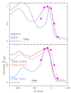 |
Fig. 3 Same as Figure 2 except that all tracers are convolved to the 38.1″ resolution of the HIFI H2O spectra. |
Water line intensities across the Horsehead PDR.
Maximum integrated line intensities toward the Horsehead PDR.
4.2 The PDR wrapper approach
Here, we also use Version 7 of the Meudon PDR code3, but to compare the outputs of the code with spatially resolved observations of edge-on structures such as the Horsehead nebula, we developed a dedicated post-processing tool: the PDR wrapper. This tool maps the 1D Meudon PDR model onto a 2D plane defined by the lines of sight and the direction of radiation propagation, under the assumption of a simplified, shell-like geometry characterized by a fixed radius of curvature.
Figure 4 depicts a typical 1D PDR model geometry as used by the Meudon PDR code, with a two-component radiation field composed of a perpendicular beamed stellar radiation field from a nearby star and an isotropic mean interstellar radiation field (ISRF). We also see the chemical stratification, with the ionization front denoting the beginning of the PDR, followed by the dissociation front (H/H2 transition) separating the atomic and molecular regions, and the C+/C/CO transition taking place deeper in the cloud, followed by the appearance of H2O molecules.
An illustration of the wrapper’s conceptual geometry is provided in Figure 5. The left panel shows a real image of the Horsehead nebula, while the middle and right panels offer a rotated side-view artistic rendition of the cloud. In this representation, the stellar radiation field is incident from the top, while the lines of sight toward the observer extend horizontally to the right. The total set of lines of sight corresponds to a vertical column of pixels in the original image, effectively forming a cut across the nebula.
The shell-like structure superimposed in the right panel models the curved PDR surface, along which the output of a single 1D Meudon PDR model is mapped. This 1D structure is effectively “swept” along the arc, assuming a constant radius of curvature. Examples of such 1D models are drawn as red vertical lines on the figure.
A run of the Meudon PDR code produces a wide range of outputs. Among these, we make use of the density profiles of the chemical species of interest, as well as the profiles of their populations in individual quantum levels. Note that by using perpendicular illumination in the PDR code to simulate irradiation by the illuminating star, each point on the surface of the resulting sphere is illuminated perpendicularly. This approach provides a more realistic representation of a stellar-illuminated surface than would do a 1D spherical PDR model, in which the illumination is assumed to be isotropic.
Once the level populations were known throughout this 2D structure, we computed the line intensities as seen by an observer along many perpendicular lines of sight. This allowed us to reconstruct the spatial variation of the line intensities from the ionization front to the core of the cloud. The line intensities were determined by solving the radiative transfer equation along each line of sight, using the level populations interpolated from the Meudon PDR model, integrating from the far side of the cloud to the edge of the PDR on the observer’s side (see Appendix A for more details).
Lines of sight shown as solid arrows in Figure 5 intersect only physically meaningful regions of the cloud where the PDR model predicts densities and level populations. In contrast, dashed lines cross into central regions not covered by the model and are excluded from further analysis.
The wrapper reconstructs the spatial emission profiles as they would appear when observing a locally curved PDR edge-on, accounting for both curvature effects and radiative transfer along the lines of sight. This method enables the generation of synthetic spatial emission profiles while avoiding the computational cost of full 2D radiative transfer, which can be prohibitive for large parameter-space explorations while maintaining a very high level of process modeling.
Examples illustrating the wrapper geometry are shown in Figure 6, where a single Meudon PDR model (Pth = 4 × 10⁶ K cm−3, G0 = 100 Habing units, Habing 1968) is projected onto shells with three different radii of curvature. The RGB composite maps simultaneously represent the abundances of the three main carbon-bearing species: red for ionized carbon (C+), green for atomic carbon (C), and blue for carbon monoxide (CO). This color-coding highlights the chemical stratification from the ionized outer layers to the molecular interior, with mixed regions appearing as intermediate colors such as yellow, cyan, or white. The observer is located at the bottom of each map, and the stellar radiation field enters from the right. These examples visualize the transition from ionized to atomic to molecular carbon, as well as the local spherical curvature along the line of sight. In this representation, radiative transfer is computed from top to bottom.
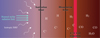 |
Fig. 4 Illustration of the geometry of 1D PDR models made with the Meudon PDR code. We show the two-component radiation field composed of a beamed part representing the stellar radiation field and an isotropic part representing the ISRF. This configuration yields the typical chemical stratification, with the ionization front denoting the beginning of the PDR, followed by the dissociation front, or H/H2 transition, and the C+/C/CO transition deeper in the cloud. H2O appears even deeper. |
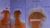 |
Fig. 5 Illustration of the geometry of the PDR wrapper. (Left panel) Image of the Horsehead nebula as seen by the Euclid space telescope (Credits: ESA/Euclid/Euclid Consortium/NASA, image processing by J.-C. Cuillandre (CEA Paris-Saclay), G. Anselmi). Notice the reference frame, with the x-axis corresponding to the direction of the lines of sight. We rotate the nebula so that the x–axis points to the right. (Middle panel) Artistic interpretation of the rotation of the Horsehead nebula, generated using OpenAI’s DALL·E model based on the first panel image. (Right panel) Geometry of the wrapping 2D model, with the star radiation field coming from the top, and examples of Meudon PDR model output overplotted as vertical red lines. Each of these lines correspond to a PDR model as represented on Fig. 4. Notice that we use the same model for each position along the cut of the cloud. The multiple lines of sight correspond to different pixels along a vertical 1D cut in the Horsehead nebula. We emphasize that only the lines of sight shown as solid lines are correctly accounted for by the model, as the central section of the nebula outside of the crescent-shaped area is not included in the computations. The geometry is assumed to be circular with a radius of curvature that remains to be determined. |
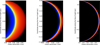 |
Fig. 6 Illustration of the wrapper geometry, showing RGB composite maps of carbon-bearing species for different radii of curvature. The color encodes the local abundances as follows: red for ionized carbon (C+), green for neutral atomic carbon (C), and blue for carbon monoxide (CO). Areas where these species coexist appear as color blends (e.g., cyan for C and CO, yellow for C+ and C, white for equal contributions). The left panel shows a curvature radius of RC = 0.05 pc, the middle to RC = 0.2 pc, and the right to RC = 0.5 pc. These maps highlight the local spherical curvature in the plane of the sky, with the observer located at the bottom of each panel and the stellar radiation field entering from the right. Radiative transfer is computed along vertical lines from top to bottom in this configuration. The abundances originate from a single Meudon PDR model (Pth = 4 × 10⁶ K cm−3, G0 = 100). The usual edge-on representation of abundances of this model can be found in Figure 10. |
4.3 Model grid and physical ingredients
As discussed in Section 4.5, reproducing the H2O emission line proved challenging. For this reason, we separate the analysis into two parts: the reproduction of the C+/C/CO transitions, based on both line intensities and spatial profiles, is presented here, while the modeling of the H2O line and its spatial distribution is treated independently.
For the first part of the analysis, we constructed a grid of isobaric Meudon PDR models coupled with the wrapper tool. The explored parameter space includes:
thermal pressures Pth = 0.5, 1, 2, 3, 4, 5, 6, 8, and 10 × 106 K cm−3; and
curvature radii RC = 0.02, 0.05, 0.1, 0.2, 0.5, and 1.0 pc.
A standard value for the interstellar radiation field of G0 = 100 Habing units is used for the models, as the line intensities of [C II] 158 μm, [C I] 609 μm, and low-J CO transitions depend only weakly on G0 in low-excitation PDRs such as the Horsehead nebula (see, e.g., Kaufman et al. 1999). This choice of G0 is motivated by multiple studies of the Horsehead nebula (e.g., Abergel et al. 2003; Habart et al. 2005; Goicoechea et al. 2009; Santa-Maria et al. 2023; Zannese et al. 2025) and the spectral type of the illuminating star, σ Ori, O 9.5 V at a projected distance of 3.5 pc. We further discuss the weak G0 dependence in Appendix C.
The models incorporate an exact radiative transfer treatment for H2 lines. This means that H2 self-shielding is calculated precisely, properly accounting for the overlap of UV pumping lines from both H and H2. This formalism also ensures that the model accurately considers the shielding of the CO UV lines by the H2 Lyman and Werner transitions.
The chemical network considers 220 species and more than 3300 reactions including a surface chemistry network for the chemistry of carbon and oxygen and the formation of mantles of H2O on the grains. The radiation field is modeled using a synthetic spectra from the POLLUX database (Palacios et al. 2010) to simulate the σ-Ori stellar spectrum. The selected parameters are Teff = 33 000 K, log (g) = 4.26 and R = 5.26 R⊙. Turbulent broadening is included with a velocity dispersion σturb = 0.38 km s−1, following Hernández-Vera et al. (2023), derived from ALMA observations of HCO+ in the Horsehead nebula. The impact of this choice on the predicted line intensities is discussed in Sect. 4.5.
4.4 Model fitting procedure and main results
The synthetic emission profiles produced by the wrapper were compared to observational data using a χ2 minimization method implemented in the pyismtools Python suite. The fitting simultaneously considered both the maximum intensities and, for the first time, the spatial separation between the emission peaks along the PDR. For the minimization, we did not use the raw output of the wrapping procedure, but rather the profiles convolved to match the native angular resolution of each tracer image. The minimum χ2 value is obtained for Pth = 4.1 × 10⁶ K cm−3 and RC = 0.057 pc, being consistent with previously published, with RC being around half the typical 0.1 pc width usually assumed in plane-parallel models of the Horsehead PDR (Figure 7).
A comparison between the best model and the observations is shown in Fig. 8. The bottom panel displays the maximum intensities of the emission lines, demonstrating excellent agreement. Model predictions are plotted as empty circles with 40% error bars, accounting for geometrical uncertainties and the complexity of the parameter space. In the top panels, we compare the full spatial emission profiles from our model to the observed profiles, even though the minimization relied solely on maximum intensities and separations between various tracers. The left panel shows the raw model profiles produced by the Wrapper, while the right panel presents the same profiles convolved to the native angular resolution of the respective tracers, as used in the minimization. As stated before, we emphasize that our modeling focuses solely on reproducing the initial rise in intensity for each emission line, since the geometrical model is physically consistent only within the computed width of the PDR.
Notably, even though only maximum positions were used for fitting, the complete spatial profiles are well reproduced. An exception is observed for the CO lines and their isotopologs, for which the observed rise in intensity near the illuminated edge is smoother than predicted. This discrepancy remains unexplained and may be due to convolution of multiple CO fronts (eg., Hernández-Vera et al. 2023).
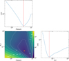 |
Fig. 7 A map of χ2 values obtained from the minimization procedure using maximum intensities and spatial separations. The best-fit model, corresponding to Pth = 4.1 × 10⁶ K cm−3, and RC = 0.057 pc, is denoted by the orange circle on the map. The constraint on RC remains weak, with the χ2 surface relatively flat in a wide valley. |
4.5 H2O emission
Figures 8 and 9 show the spatial emission profiles (after the wrapping procedure, and convolution to the native angular resolution of each tracer) and the maximum intensities including the H2O 110–101 line, for the model: Pth = 4 × 10⁶ K cm−3, G0 = 100, and RC = 0.05 pc. For water, the model predicts an intensity about 20 times higher than the observed value, and a spatial distribution of the emission much more recessed into the cloud. Models with lower G0 values provide a somewhat better fit to the observations. However, the model water line intensity is stil a factor of seven higher than the observations (see Fig. C.2 in Appendix C).
There are several possible explanations for these discrepancies. First, H2O excitation is very sensitive to radiative transfer effects (Poelman & Spaans 2006; Gonzalez Garcia et al. 2008), such as nonlocal pumping by warm dust emission. Also, the line is strongly optically thick, with optical depths of the order of 103, so the emergent intensity is determined by the local excitation temperature at the τ ~ 1 surface. The location of this surface is highly sensitive to both the H2O abundance profile and the line width, which is controlled by turbulent broadening. A smaller turbulent velocity leads to a narrower line, increasing the opacity, and thus shifting the τ ~ 1 surface outward, closer to the cloud edge where the excitation temperature is lower, thereby decreasing the emergent intensity.
To test the sensitivity of the results to turbulent velocity dispersion, we also considered the smaller value of σturb = 0.225 km s−1 derived from the analysis of Gerin et al. (2009), who derived this value for the Horsehead from HCO observations combining Plateau de Bure Interferometer (PdBI) and IRAM-30m data. In this case the predicted intensity decreases by about 24%, from 7.58 × 10⁻⁷ erg cm−2 s−1 sr−1 to 5.75 × 10⁻⁷ erg cm−2 s−1 sr−1. Both predictions remain far above the observed value of 3.67 × 10⁻⁸ erg cm−2 s−1 sr−1. For the other tracers, we find that decreasing the turbulent velocity has almost no effect on [C II] and [C I], but it reduces the CO line intensities by ~20%, thereby slightly improving the agreement with the observations.
In addition, the intensity of optically thick lines varies non linearly with the abundance profile. A small change in the predictions of the density of H2O can result in significant variations in line intensities. We checked that our model is perfectly in line with the classical PDR model of the chemistry of H2O (Hollenbach et al. 2009), except that surface chemical data (e.g., binding energies) have been updated and the modeling of some processes has been modernized (Cuppen et al. 2017). Also, we know that the model reproduces H2O line intensities in more intense PDRs such as the Orion Bar (Putaud et al. 2019). This may suggest that particular processes may be at work in the Horsehead, possibly involving grains with unusual properties, whether in composition or size distribution.
The detailed analysis of dust and H2 emission recently observed by JWST in the Horsehead nebula could help clarify this issue (Abergel et al. 2024). These findings also highlight the need to refine the modeling of chemical processes on interstellar grains, particularly by acknowledging that the physical conditions of these grains likely differ from those under which binding energies and process efficiencies, such as photo-desorption yields, are measured in laboratory experiments (Hacquard et al. 2024). For instance, given the diversity of interstellar grain types, it would be more realistic to adopt distributions of binding energies for adsorbed species instead of single fixed values. However, this would require the development of new formalisms to accurately simulate surface chemistry. Last but not least, another factor to consider is the geometry of the emission and nonlocal radiative transfer effects: the discrepancy between models and observations may well arise from scattering of the radiation emitted by water molecules, as discussed in the following section.
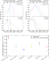 |
Fig. 8 (Top) Spatial profiles of normalized emission line intensities observed in the Horsehead nebula, compared with predictions from a Meudon PDR model with Pth = 4 × 10⁶ K cm−3 and G0 = 100, wrapped in a locally spherical cloud with a curvature radius RC = 0.05 pc. These conditions correspond to commonly adopted literature values. The left panels show the raw profiles from the wrapping procedure, while the right panels present the same profiles convolved to the native angular resolution of each tracer. In those figures, the radiation field comes from the right. (Bottom) Observed maximum intensities of various tracers (colored crosses) compared to model predictions (circles with error bars). All tracers are well reproduced, except for H2O, where the model overestimates the observed maximum intensity by an order of magnitude. |
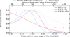 |
Fig. 9 Spatial profiles of normalized emission line intensities observed in the Horsehead nebula, compared to predictions from Meudon PDR model with Pth = 4 × 10⁶ K cm−3 and G0 = 100, wrapped in a locally spherical cloud with curvature radius RC = 0.05 pc. The profiles are convolved to the native angular resolution of the tracer maps. On this figure, the radiation field comes from the right. We observed a significant shift between the observed H2O profile and the model, the latter being much deeper in the cloud. |
5 Scattered o-H2O 110–101 557 GHz line emission by low-density warm envelopes
In this section, we describe a plausible scenario explaining why the o-H2O 110–101 557 GHz line emission is more extended toward the rim of the PDR than the 12CO (2–1) emission, and why it nearly coincides with the [CII] 158 μm emission when convolved to the same low angular resolution (~38″), which traces lower-density gas at the rim of the PDR (Pabst et al. 2017; Bally et al. 2018). Firstly, we note that a steep gas density gradient exists in the Horsehead, with densities varying from the PDR/H II interface (nH ≈ a few 103 cm−3, T ≳ 100 K) to the more shielded, cold molecular cores (nH ≈ a few 105 cm−3, T ≈ 20 K) (e.g., Habart et al. 2005; Pety et al. 2007; Gerin et al. 2009; Goicoechea et al. 2009; Hernández-Vera et al. 2023). The nearly edge-on orientation of the PDR allows these different environments to be partially spatially resolved.
Our PDR models (Sect. 4.5) predict that the peak of the water vapor abundance, reaching 2.6 × 10⁻⁷, occurs at AV ~ 3 mag, well beyond the CO/C transition layer of the PDR, as can be seen on Figure 10 showing the edge-on Meudon PDR model output (thus without the wrapping). As a reference, models from Putaud et al. (2019) yielded a comparable abundance of H2O of 2 × 10⁻⁷, that occurred at AV ~ 9 mag in the Orion Bar, due to the substantially stronger radiation field. Our water abundance peak roughly corresponds to the point where the rate of gas-phase O atoms sticking to grains equals the photo-desorption rate of water molecules from icy grain surfaces. At this depth, the gas temperature is approximately 40 K, and the H2O peak lies deeper than the 12CO abundance peak. In this region of the PDR, the H2O abundance profile closely resembles that of C18O. Hence, contrary to observations, one would expect the o-H2O 557 GHz emission to be as extended as the C18O (2–1) emission. In contrast to C18O, however, H2O starts to form close to the PDR surface, ahead of the CO/C transition, where the C+ abundance is much greater than that of CO, temperatures are high, and densities are lower than at the H2O abundance peak. With this in mind, one can approximate the H2O line radiative transfer problem in the Horsehead using a two-component model: a denser, moderately cold PDR component with a large H2O column density (in the line of sight), surrounded by a lower-density, warm envelope with a lower H2O column density. This envelope represents the bright [CII]158 μm but faint 12CO (2–1) emission edge of the PDR (e.g., Pabst et al. 2017; Hernández-Vera et al. 2023).
Owing to the very high critical density for collisional excitation, ncr (110–101) ≃ 108 cm−3, and the elevated 557 GHz line opacity for moderate H2O column densities, the excitation of the 110–101 transition is very subthermal (nH ≪ ncr) (see, e.g., Flagey et al. 2013), which implies Tex ≪ T, and is prone to nonlocal radiative effects such as line resonant scattering by low-density envelopes containing water vapor. In such envelopes, the local o-H2O 557 GHz line emission is negligible because Tex → Tcmb. However, when o-H2O 557 GHz line photons emitted by the deeper PDR layers diffuse through the envelope, they are self-absorbed and re-emitted by water molecules, which increases Tex in the low-density gas and scatters the emission to greater distances. This produces an impression of a more extended spatial distribution of H2O emission. While this scattering process has been invoked to explain the extended distribution and anomalous J = 1–0 line intensity ratios of very polar molecules such as HCO+ or HCN in dark clouds (i.e., rotational transitions with a high ncr; Langer et al. 1978; Walmsley et al. 1982; Cernicharo et al. 1984; Gonzalez-Alfonso & Cernicharo 1993; Goicoechea et al. 2022), all these studies required cold envelopes. The interesting property of H2O is that the critical density of the ground-state 110–101 transition is at least 3 orders of magnitude higher than that of HCN and HCO+ J = 1–0. As we demonstrate below, this implies that the excitation temperature of the 110–101 transition remains very low even at high gas temperatures, provided that the gas density is significantly lower than the effective critical density of this transition. In this case, a warm/hot envelope containing moderately water vapor abundances will produce self-absorption and resonant scattering due to very low excitation temperature of the 110–101 in the envelope. This nonlocal radiative effect cannot be reproduced by standard (local) escape probability methods.
To investigate the impact of line scattering on the emergent H2O line intensities, we use a nonlocal and non-LTE Monte Carlo radiative transfer code (see Goicoechea et al. 2006, 2022) and develop a “simple” two-component model of the water vapor line emission adapted to the physical conditions known to exist in the Horsehead PDR. We used the H2O–H2 inelastic collision rate coefficients of Daniel et al. (2011, 2012). Following a large list of observational studies of this source, we adopt nH=6×104 cm−3 and T =40 K for the dense PDR component, and nH=6×103 cm−3, T =60 K, and for the extended envelope near the PDR/HII region interface. We found a good match to the observed line intensities by adopting a (beam-averaged) line-of-sight o-H2O column densities, N(o-H2O) ≃ 4.3×1013 cm−2 and N(o-H2O) ≃ 1.7×1013 cm−2 in these two components, respectively. These models include thermal, microturbulent, and line opacity broadening. To reproduce the observed line-widths, we adopt σturb ≃ 0.4 km s−1 in the dense PDR and σturb ≃ 1 km s−1 in the extended envelope. An increased velocity dispersion in the envelope diminishes the depth of the 557 GHz self-absorption line dip. Figure 11 shows the resulting line and radial Tex (110–101) profiles. The blue curves represent a model of the dense PDR component-only, while the red curves represent a model of the low-density envelope-only. The black curves represent the two-component model.
Due to the low gas density, the envelope-only model shows highly subthermal (Tex ≃ 3.2 K) line emission, despite the moderate gas temperatures. Thus, the predicted o-H2O 557 GHz line intensities are very faint (a few millikelvins) and would remain undetectable by Herschel/HIFI. The dense-PDR-only alone, with and order of magnitude higher gas density and a lower temperature (closer to the energy of the upper level 110), leads to more efficient collisional excitation and thus increased excitation temperatures (Tex ~ 4.5–5.5 K). In addition, the o-H2O 557 GHz line from the dense component is optically thick, which produces line opacity broadening and line-trapping (i.e., an increase of Tex at low radii despite the gas density is constant). Compared to the envelope-only model, the two-component model (black curves) has different excitation conditions in the envelope region (R > RdensePDR). The absorption and reemission of o-H2O 557 GHz line photons has two consequences: (i) It reduces the apparent o-H2O 557 GHz line intensity toward the dense component, and (ii) it increases Tex (110–101) in the envelope to levels that produce detectable scattered o-H2O 557 GHz line emission at R > RdensePDR. This is a purely radiative effect and leads to o-H2O 557 GHz line emission beyond the dense PDR component. This scenario would imply that our detection of the o-H2O 557 GHz emission at the rim of the PDR is scattered emission from deeper layers of the PDR.
Figure 12 shows the predicted radial o-H2O 110–101 integrated line intensities, with the black curves representing the two-component model. This model results in detectable o-H2O 557 GHz emission that is more extended than the dense PDR region. It also results in an decrease in the o-H2O 557 GHz line intensity for line of sights toward the core (e.g., for R/RdensePDR = 0). This simple two-component model reasonably fits the observed o-H2O 557 GHz line intensities across the PDR (magenta-filled circles in Fig. 12). We recall that a necessary condition for this radiative effect to occur is the presence of an extended, low-density envelope (lower excitation) containing moderate amounts of water vapor, as predicted by our PDR photochemical model. The size of the H2O scattered emission region and the degree of line self-absorption ultimately depends in the exact physical conditions and water vapor abundance in the different components. We note that resonant scattering does not affect the excitation or emission of low-critical-density transitions (e.g., low-J CO, [C II], or [C I] lines). Indeed, most of the C18O 2–1 emission originates in the dense PDR interior, while any C18O present in the envelope will be excited collisionally (Tex ≃ Tk) and not radiatively. As the line emission from the dense PDR is optically thin, this emission is not self-absorbed. For C+, the [C II] 158 μm line (also collisionally excited) arises mainly from the foreground envelope. These two cases, both with ncr of a few 103 cm−3, are presented in Appendix B.
In summary, our simple model captures the average physical conditions and H2O column densities within the large Herschel/HIFI beam. Higher angular resolution observations of water vapor will be necessary to properly resolve the size of each component and to account for the gradients in physical conditions and water abundance.
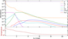 |
Fig. 10 Abundances of key species with respect to hydrogen nuclei (top panel) and gas temperature (bottom panel) profiles of the Horsehead nebula model with Pth = 4 × 10⁶ K cm−3, G0 = 100, computed with the Meudon PDR code (no wrapping or convolution procedure is applied to these profiles). The H/H2 transition can be seen to take place at around AV ~ 0.06 mag, the C+/C/CO transition is at AV ~ 1.7 mag, and the peak of H2O abundance is reached at an AV ~ 3 mag. |
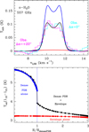 |
Fig. 11 Two-component, nonlocal radiative transfer models adapted to the physical conditions in the Horsehead. The upper panel shows the o-H2O 557 GHz synthetic line profiles (continuous curves) and observed line profiles (histograms) at the emission peak. The lower panel shows the predicted excitation temperatures of the 110–101 transition. The blue curves represent the model of the dense PDR component alone. The red curves represent the model of the low-density envelope alone, while the black curves represent the two-component model. |
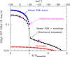 |
Fig. 12 Same as the lower panel of Fig. 11 but showing the predicted radial o-H2O 110–101 integrated line intensities. The magenta-filled circles represent the observed line intensities across the Horsehead PDR, with the peak position at Δα = +20″. |
6 Summary and conclusions
We have analyzed archival Herschel observations of water emission toward the Horsehead PDR, along with supporting ground-based and airborne observations of CO isotopologs and fine structure lines of ionized and atomic carbon. The main results of this study can be summarized as follows:
Water emission in the Horsehead nebula is very weak and, surprisingly, extends outward beyond other PDR tracers, such as CO isotopologs or [C I] 609 μm, and as far out as [C II] 158 μm;
We developed a PDR wrapper to model line emission from 3D objects illuminated by a flux of UV photons. PDR modeling shows that the [C II], [C I], and CO isotopolog intensities and spatial profiles provide strong constraints on the thermal pressure (Pth = 4 × 10⁶ K cm−3), but not on G0. A model with published source parameters provides a reasonable fit to the data, while underestimating the intensities of the [C II] and CO J = 4–3 lines by a factor of ~2.5. Spatial profiles are also well reproduced, except for CO isotopologs, where the increase on the illuminated side of the PDR is steeper than observed;
Water vapor abundance in the PDR model reaches 3.6 × 10⁻⁷ at AV ~ 3 mag. However, the ground state o-H2O 557 GHz line is systematically overestimated by the models by at least a factor of 7 for any values of the model parameters. This line has a very high optical depth, ~10, and the emergent line intensity is sensitive to radiative transfer effects and the assumed turbulent line width. Nevertheless, the PDR modeling suggests that some ingredients describing the processes that lead to the formation and destruction of water ice on grain surfaces are missing in the model;
We demonstrate that scattering of photons by water molecules in a low-density envelope surrounding the dense PDR provides a plausible explanation for the observed spatial extent of the water emission. While an isobaric Meudon PDR model naturally includes a low-density, warm envelope, the local escape and radiative transfer formalism in the code does not treat correctly the resonant scattering of water photons by the outer, lower-density gas layers.
The PDR wrapper developed here will be a powerful tool for analyzing future high angular resolution observations of molecular tracers in the Horsehead nebula obtained using ground-based millimeter-wave interferometers. Such observations will much better delineate the spatial stratification among various PDR tracers than the single-dish observaions presented here, providing more stringent constraints on the physical parameters.
Acknowledgements
This research was carried out at the Jet Propulsion Laboratory, California Institute of Technology, under a contract with the National Aeronautics and Space Administration (80NM0018D0004). D.C.L. acknowledge financial support from the National Aeronautics and Space Administration (NASA) Astrophysics Data Analysis Program (ADAP). HIFI was designed and built by a consortium of institutes and university departments from across Europe, Canada, and the United States (NASA) under the leadership of SRON, Netherlands Institute for Space Research, Groningen, The Netherlands, and with major contributions from Germany, France, and the US. This research has made use of the NASA/IPAC Infrared Science Archive, which is funded by the National Aeronautics and Space Administration and operated by the California Institute of Technology. JRG thanks the Spanish MCINN for funding support under grant PID2023-146667NB-I00. This work was supported by the Thematic Action “Physique et Chimie du Milieu Interstellaire” (PCMI) of INSU Programme National “Astro”, with contributions from CNRS Physique & CNRS Chimie, CEA, and CNES. This research was achieved using the POLLUX database (pollux.oreme.org) operated at LUPM (Université de Montpellier – CNRS, France) with the support of the PNPS and INSU. V.M. and J.R.G. thank the Spanish MCINN for funding support under grant PID2023-146667NB-I00. We thank an anonymous referee for helpful comments.
References
- Abergel, A., Misselt, K., Gordon, K., et al. 2024, A&A, 687, A4 [NASA ADS] [CrossRef] [EDP Sciences] [Google Scholar]
- Abergel, A., Teyssier, D., Bernard, J. P., et al. 2003, A&A, 410, 577 [CrossRef] [EDP Sciences] [Google Scholar]
- Bally, J., Chambers, E., Guzman, V., et al. 2018, AJ, 155, 80 [Google Scholar]
- Bockelée-Morvan, D., Lis, D. C., Wink, J. E., et al. 2000, A&A, 353, 1101 [Google Scholar]
- Cernicharo, J., Castets, A., Duvert, G., & Guilloteau, S. 1984, A&A, 139, L13 [NASA ADS] [Google Scholar]
- Cubick, M., Stutzki, J., Ossenkopf, V., Kramer, C., & Röllig, M. 2008, A&A, 488, 623 [NASA ADS] [CrossRef] [EDP Sciences] [Google Scholar]
- Cuppen, H. M., Walsh, C., Lamberts, T., et al. 2017, Space Sci. Rev., 1 [Google Scholar]
- Daniel, F., Dubernet, M. L., & Grosjean, A. 2011, A&A, 536, A76 [NASA ADS] [CrossRef] [EDP Sciences] [Google Scholar]
- Daniel, F., Goicoechea, J. R., Cernicharo, J., Dubernet, M. L., & Faure, A. 2012, A&A, 547, A81 [NASA ADS] [CrossRef] [EDP Sciences] [Google Scholar]
- Daniel, F., Faure, A., Dagdigian, P. J., et al. 2015, MNRAS, 446, 2312 [NASA ADS] [CrossRef] [Google Scholar]
- de Graauw, T., Helmich, F. P., Phillips, T. G., et al. 2010, A&A, 518, L6 [NASA ADS] [CrossRef] [EDP Sciences] [Google Scholar]
- Drozdovskaya, M. N., van Dishoeck, E. F., Rubin, M., Jørgensen, J. K., & Altwegg, K. 2019, MNRAS, 490, 50 [Google Scholar]
- Faure, A., Gorfinkiel, J. D., & Tennyson, J. 2004, MNRAS, 347, 323 [NASA ADS] [CrossRef] [Google Scholar]
- Flagey, N., Goldsmith, P. F., Lis, D. C., et al. 2013, ApJ, 762, 11 [NASA ADS] [CrossRef] [Google Scholar]
- Gerin, M., Goicoechea, J. R., Pety, J., & Hily-Blant, P. 2009, A&A, 494, 977 [NASA ADS] [CrossRef] [EDP Sciences] [Google Scholar]
- Goicoechea, J. R., Pety, J., Gerin, M., et al. 2006, A&A, 456, 565 [NASA ADS] [CrossRef] [EDP Sciences] [Google Scholar]
- Goicoechea, J. R., Pety, J., Gerin, M., Hily-Blant, P., & Le Bourlot, J. 2009, A&A, 498, 771 [NASA ADS] [CrossRef] [EDP Sciences] [Google Scholar]
- Goicoechea, J. R., Lique, F., & Santa-Maria, M. G. 2022, A&A, 658, A28 [NASA ADS] [CrossRef] [EDP Sciences] [Google Scholar]
- Gonzalez-Alfonso, E., & Cernicharo, J. 1993, A&A, 279, 506 [NASA ADS] [Google Scholar]
- Gonzalez Garcia, M., Le Bourlot, J., Le Petit, F., & Roueff, E. 2008, A&A, 485, 127 [NASA ADS] [CrossRef] [EDP Sciences] [Google Scholar]
- Guzmán, V., Pety, J., Goicoechea, J. R., Gerin, M., & Roueff, E. 2011, A&A, 534, A49 [NASA ADS] [CrossRef] [EDP Sciences] [Google Scholar]
- Guzmán, V., Pety, J., Gratier, P., et al. 2012, A&A, 543, L1 [CrossRef] [EDP Sciences] [Google Scholar]
- Guzmán, V. V., Goicoechea, J. R., Pety, J., et al. 2013, A&A, 560, A73 [Google Scholar]
- Habart, E., Abergel, A., Walmsley, C. M., Teyssier, D., & Pety, J. 2005, A&A, 437, 177 [NASA ADS] [CrossRef] [EDP Sciences] [Google Scholar]
- Habing, H. J. 1968, Bull. Astron. Inst. Netherlands, 19, 421 [Google Scholar]
- Hacquard, A. B., Basalgète, R., Del Fré, S., et al. 2024, J. Chem. Phys., 161, 184306 [Google Scholar]
- Hernández-Vera, C., Guzmán, V. V., Goicoechea, J. R., et al. 2023, A&A, 677, A152 [NASA ADS] [CrossRef] [EDP Sciences] [Google Scholar]
- Hollenbach, D., Kaufman, M. J., Bergin, E. A., & Melnick, G. J. 2009, ApJ, 690, 1497 [NASA ADS] [CrossRef] [Google Scholar]
- Joblin, C., Bron, E., Pinto, C., et al. 2018, A&A, 615, A129 [NASA ADS] [CrossRef] [EDP Sciences] [Google Scholar]
- Kaufman, M. J., Wolfire, M. G., Hollenbach, D. J., & Luhman, M. L. 1999, ApJ, 527, 795 [Google Scholar]
- Langer, W. D., Wilson, R. W., Henry, P. S., & Guelin, M. 1978, ApJ, 225, L139 [NASA ADS] [CrossRef] [Google Scholar]
- Le Petit, F., Nehmé, C., Le Bourlot, J., & Roueff, E. 2006, ApJS, 164, 506 [NASA ADS] [CrossRef] [Google Scholar]
- Melnick, G. J., Tolls, V., Snell, R. L., et al. 2011, ApJ, 727, 13 [Google Scholar]
- Melnick, G. J., Tolls, V., Snell, R. L., et al. 2020, ApJ, 892, 22 [CrossRef] [Google Scholar]
- Pabst, C. H. M., Goicoechea, J. R., Teyssier, D., et al. 2017, A&A, 606, A29 [NASA ADS] [CrossRef] [EDP Sciences] [Google Scholar]
- Palacios, A., Gebran, M., Josselin, E., et al. 2010, A&A, 516, A13 [NASA ADS] [CrossRef] [EDP Sciences] [Google Scholar]
- Peeters, E., Habart, E., Berné, O., et al. 2024, A&A, 685, A74 [NASA ADS] [CrossRef] [EDP Sciences] [Google Scholar]
- Pety, J., Teyssier, D., Fossé, D., et al. 2005, A&A, 435, 885 [NASA ADS] [CrossRef] [EDP Sciences] [Google Scholar]
- Pety, J., Goicoechea, J. R., Hily-Blant, P., Gerin, M., & Teyssier, D. 2007, A&A, 464, L41 [NASA ADS] [CrossRef] [EDP Sciences] [Google Scholar]
- Pety, J., Gratier, P., Guzmán, V., et al. 2012, A&A, 548, A68 [NASA ADS] [CrossRef] [EDP Sciences] [Google Scholar]
- Philipp, S. D., Lis, D. C., Güsten, R., et al. 2006, A&A, 454, 213 [NASA ADS] [CrossRef] [EDP Sciences] [Google Scholar]
- Pilbratt, G. L., Riedinger, J. R., Passvogel, T., et al. 2010, A&A, 518, L1 [NASA ADS] [CrossRef] [EDP Sciences] [Google Scholar]
- Pilleri, P., Fuente, A., Cernicharo, J., et al. 2012, A&A, 544, A110 [NASA ADS] [CrossRef] [EDP Sciences] [Google Scholar]
- Poelman, D. R., & Spaans, M. 2006, A&A, 453, 615 [NASA ADS] [CrossRef] [EDP Sciences] [Google Scholar]
- Putaud, T., Michaut, X., Le Petit, F., Roueff, E., & Lis, D. C. 2019, A&A, 632, A8 [NASA ADS] [CrossRef] [EDP Sciences] [Google Scholar]
- Santa-Maria, M. G., Goicoechea, J. R., Pety, J., et al. 2023, A&A, 679, A4 [NASA ADS] [CrossRef] [EDP Sciences] [Google Scholar]
- Tielens, A. G. G. M., & Hollenbach, D. 1985a, ApJ, 291, 722 [Google Scholar]
- Tielens, A. G. G. M., & Hollenbach, D. 1985b, ApJ, 291, 747 [NASA ADS] [CrossRef] [Google Scholar]
- van Dishoeck, E. F., Herbst, E., & Neufeld, D. A. 2013, Chem. Rev., 113, 9043 [Google Scholar]
- van Dishoeck, E. F., Kristensen, L. E., Mottram, J. C., et al. 2021, A&A, 648, A24 [NASA ADS] [CrossRef] [EDP Sciences] [Google Scholar]
- Walmsley, C. M., Churchwell, E., Nash, A., & Fitzpatrick, E. 1982, ApJ, 258, L75 [NASA ADS] [CrossRef] [Google Scholar]
- Zannese, M., Guillard, P., Abergel, A., et al. 2025, A&A, 704, A202 [NASA ADS] [CrossRef] [EDP Sciences] [Google Scholar]
Appendix A Presentation of the PDR wrapper
A.1 Aims of the code
The Meudon PDR code (Le Petit et al. 2006) models interstellar clouds as 1D, plane-parallel slabs, infinite and homogeneous along their surface. It computes the steady-state gas and chemistry structure along the normal to the surface, as a function of optical depth, and predicts line intensities emerging from the illuminated side. Level excitation is determined at each position in the cloud by solving the non-LTE problem, taking into account radiative and collisional transitions, as well as chemical formation and destruction in specific levels. The algorithm that computes the stationary level populations is intimately coupled to the solution of the radiative transfer equation, as described in Gonzalez Garcia et al. (2008). The algorithm considers non local pumping in the continuum (dust emission plus CMB). For example, the radiation field emitted by warm dust at the edge of the PDR can pump transitions deeper in the cloud where dust is cold. Concerning line emission, the algorithm uses a on the spot approximation meaning that the line can be re-absorbed, but only locally. For H2O, the code considers inelastic collisions with H (Daniel et al. 2015), He (scaling of the collision rates with H), ortho and para H2 (Daniel et al. 2011), e− (Faure et al. 2004).
Edge-on clouds illuminated from the side reveal PDR stratification through spatially offset line emissions. Although their complex geometry requires simplifications, the Meudon code allows for a detailed treatment of microphysics, chemistry, and radiative transfer. Extending this approach to a full 2D model with the same level of refinement in the treatment of physical processes would, however, be computationally prohibitive.
When the PDR width is small compared to the cloud radius, radiative transfer can be simplified by mapping the 1D model onto a 2D spherical geometry. This is the basis of the PDR Wrapper, which reconstructs line emission by solving radiative transfer along each line of sight through a spherical cloud cross-section.
A.2 Geometry
We assumed a locally spherical curvature for the cloud surface, with center of curvature O and radius RC. The PDR is modeled as the outermost shell of thickness dPDR ≪ RC.
The radiation field is assumed constant and perpendicular to the line of sight. The cloud has a curvature radius RC and a constant horizontal thickness dPDR. It is modeled as the shell between two arcs of radius RC, with centers shifted horizontally by dPDR (Fig. A.1). For a point on the outer arc making an angle α with the horizontal, the depth d from the illuminated edge is
![Mathematical equation: $\[d=R_{\mathrm{C}}(\cos~ \alpha-1)+b,\]$](/articles/aa/full_html/2026/02/aa56926-25/aa56926-25-eq2.png) (A.1)
(A.1)
with sin α = s/RC. The expression for smax remains unchanged, while:
![Mathematical equation: $\[s_{\mathrm{min}}(b)= \begin{cases}0 & \text { if } b<d_{\mathrm{PDR}}, \\ \sqrt{R_{\mathrm{C}}^2-\left(R_{\mathrm{C}}-b+d_{\mathrm{PDR}}\right)^2} & \text { otherwise }.\end{cases}\]$](/articles/aa/full_html/2026/02/aa56926-25/aa56926-25-eq3.png) (A.2)
(A.2)
A.3 Radiative transfer
Each image pixel integrates emission and absorption along a single line of sight. Our model solves the radiative transfer equation along multiple, parallel, and independent lines of sight across the cloud.
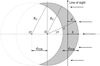 |
Fig. A.1 Horizontal geometry used for the wrapping of Meudon PDR models. The beamed ISRF remains perpendicular to the line of sight. |
The goal is to compute the intensity of a user-selected line at frequency νul, where u and l are the upper and lower energy levels, respectively. Accounting for spontaneous emission (Aul), stimulated emission (Bul), and absorption (Blu), the radiative transfer equation reads
![Mathematical equation: $\[\frac{\mathrm{d} I_\nu}{\mathrm{~d} s}=\frac{\phi\left(\nu, \nu_{u l}, s\right)}{4 \pi} h \nu\left[A_{u l} n_u(s)+\left(B_{u l} n_u(s)-B_{l u} n_l(s)\right) I_\nu\right],]$](/articles/aa/full_html/2026/02/aa56926-25/aa56926-25-eq4.png) (A.3)
(A.3)
where nu(s) and nl(s) are the level populations along the line of sight.
The normalized line profile ϕ is assumed Doppler-broadened due to thermal motions and turbulence, and is given by:
![Mathematical equation: $\[\phi\left(\nu, \nu_{u l}, s\right)=\frac{1}{\sigma_{\nu_{u l}}(s) \sqrt{2 \pi}} \exp \left[-\frac{\left(\nu-\nu_{u l}\right)^2}{2 \sigma_{\nu_{u l}}^2(s)}\right],\]$](/articles/aa/full_html/2026/02/aa56926-25/aa56926-25-eq5.png) (A.4)
(A.4)
![Mathematical equation: $\[\sigma_{\nu_{u l}}=\frac{\sqrt{2}}{2} \frac{\nu_{u l}}{c} \sqrt{\frac{2 k_{\mathrm{B}} T}{m}+\sigma_{\text {turb}}^2},\]$](/articles/aa/full_html/2026/02/aa56926-25/aa56926-25-eq6.png) (A.5)
(A.5)
where the normalization relation is
![Mathematical equation: $\[\int_0^{+\infty} \phi\left(\nu, \nu_{u l}, s\right) \mathrm{d} \nu=1.\]$](/articles/aa/full_html/2026/02/aa56926-25/aa56926-25-eq7.png) (A.6)
(A.6)
The Einstein relations (valid when working with Iν) are:
![Mathematical equation: $\[B_{u l}=\frac{c^2}{2 h \nu_{u l}^3} A_{u l}, \quad B_{l u}=\frac{g_u}{g_l} B_{u l}.\]$](/articles/aa/full_html/2026/02/aa56926-25/aa56926-25-eq8.png) (A.7)
(A.7)
Rewriting the transfer equation as:
![Mathematical equation: $\[\frac{\mathrm{d} I_\nu}{\mathrm{~d} s}=\epsilon_\nu-\alpha_\nu I_\nu,\]$](/articles/aa/full_html/2026/02/aa56926-25/aa56926-25-eq9.png) (A.8)
(A.8)
where we define the emissivity and absorption coefficients:
![Mathematical equation: $\[\epsilon_\nu=\frac{\phi\left(\nu, \nu_{u l}, s\right)}{4 \pi} h \nu A_{u l} n_u(s),\]$](/articles/aa/full_html/2026/02/aa56926-25/aa56926-25-eq10.png) (A.9)
(A.9)
![Mathematical equation: $\[\alpha_\nu=\frac{\phi\left(\nu, \nu_{u l}, s\right)}{4 \pi} h \nu\left[B_{l u} n_l(s)-B_{u l} n_u(s)\right].\]$](/articles/aa/full_html/2026/02/aa56926-25/aa56926-25-eq11.png) (A.10)
(A.10)
The formal solution is
![Mathematical equation: $\[I_\nu(s)=\int_{s_{\min }}^s \epsilon_\nu\left(s^{\prime}\right) e^{-\tau_\nu\left(s^{\prime}\right)} \mathrm{d} s^{\prime}, \quad \tau_\nu(s)=\int_{s_{\min }}^s \alpha_\nu\left(s^{\prime}\right) \mathrm{d} s^{\prime}.\]$](/articles/aa/full_html/2026/02/aa56926-25/aa56926-25-eq12.png) (A.11)
(A.11)
Finally, the total emergent intensity along the line of sight (impact parameter b) is obtained by frequency integration:
![Mathematical equation: $\[I(b)=\int_0^{+\infty} I_\nu(b) \mathrm{d} \nu.\]$](/articles/aa/full_html/2026/02/aa56926-25/aa56926-25-eq13.png) (A.12)
(A.12)
A.4 Convolution with instrumental PSF
The PSF (point spread function) characterizes the response of an instrument to a point-like source. It defines the instrument angular resolution. To model the instrumental response to the spatial profiles, we convolve I(b) or N(b) with a Gaussian kernel:
![Mathematical equation: $\[g(x)=\frac{1}{\sigma \sqrt{2 \pi}} \exp \left(-\frac{x^2}{2 \sigma^2}\right),\]$](/articles/aa/full_html/2026/02/aa56926-25/aa56926-25-eq14.png) (A.13)
(A.13)
where x is the distance to the center of the PSF, and σ the standard deviation of the PSF, linked to the full width half maximum (FWHM) of the instrument:
![Mathematical equation: $\[\sigma=\frac{\mathrm{FWHM}}{2 \sqrt{2 ~ln~2}}.\]$](/articles/aa/full_html/2026/02/aa56926-25/aa56926-25-eq15.png) (A.14)
(A.14)
The convolution product is thus:
![Mathematical equation: $\[(I * g)(b)=\int_{-\infty}^{+\infty} I(b^{\prime}) g(b-b^{\prime})~\mathrm{d} b^{\prime}.\]$](/articles/aa/full_html/2026/02/aa56926-25/aa56926-25-eq16.png) (A.15)
(A.15)
In practice, the integral is limited to the range of b plus or minus 3 times the standard deviation σ of the gaussian kernel. Outside of the range of b, the intensity is taken as a linear extrapolation of the profile.
Appendix B Two-component model of the C18O 2–1 and [C II] 158 μm line emission in the Horsehead
In this Appendix, we present the results of applying the simple two-component model to C18O and C+. These two species serve as examples of line emission arising predominantly from the dense PDR and from the extended PDR envelope, respectively. In contrast to H2O, the C18O 2–1 and [C II] 158 μm lines are low-critical-density transitions, with ncr of only a few ×103 cm−3. This means that they are collisionally excited (Tex ≃ Tk) in the envelope and therefore do not scatter line emission originating from the dense PDR, which we demonstrate here. These representative models are designed to reproduce the observed line peak intensities and their approximate spatial distribution qualitatively. Specifically, C18O 2–1 peaks toward the dense PDR, while [C II] 158 μm peaks further ahead. The physical conditions and line-widths are the same as those of the H2O models (Sect. 5). Following the PDR model, the adopted C18O abundances relative to H nuclei are 1.5 × 10⁻⁷ in the dense PDR and 1 × 10⁻⁸ in the envelope. For C+, we adopt 2×10⁻⁴ in the envelope and 2×10⁻⁶ in the dense PDR. These choices successfully reproduce the observed intensity levels, indicating that the simple two-component model is globally realistic.
Figure B.1 shows the predicted radial profiles of the C18O 2–1 and [C II] 158 μm line intensities for the dense PDR-only model (blue squares), the envelope-only model (red squares), and the combined dense PDR plus envelope model (black squares). This figure is analogous to Fig. 12 for the o-H2O 557 GHz line. As C18O 2–1 and [C II] 158 μm lines are collisionally excited, the envelope does not produce scattering of line photons emitted in the dense PDR (i.e., the red and black curves in the envelope are the same). Furthermore, the C18O 2–1 line is optically thin, so the emission from the dense PDR is not self-absorbed. For C+, the abundance in the dense PDR is much lower than toward the envelope, so any emission along the line of sight originates from the foreground envelope.
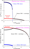 |
Fig. B.1 Two-component, nonlocal non-LTE radiative transfer model of the Horsehead applied to C18O and C+. The horizontal magenta line shows the observed maximum line intensities of the C18O 2–1 (upper panel) and [C II] 158 μm (lower panel) lines (Table 2). |
Appendix C Weak dependence of the model results on G0
We discuss here the dependence of the model line intensities on the interstellar radiation field scaling factor, G0. As shown below, the best fit PDR wrapper model suggests a weak dependence of the model line intensities on G0, with the best fit G0 value that appears low compared to the nominal value of G0 ~ 100 derived in previous studies of the Horsehead nebula (Abergel et al. 2003; Habart et al. 2005; Goicoechea et al. 2009; Santa-Maria et al. 2023), and implied by the spectral type of the ionizing star, σ Ori, O 9.5 V at a projected distance of 3.5 pc. While observations suggest that the ionizing star is located behind the nebula, the angle is quite oblique (see Fig. 13 of Abergel et al. 2024). Therefore, the actual distance is expected to be close to the projected distance. Zannese et al. (2025) also favor G0 = 100 in their analysis of new JWST observations of H2 line emission in the Horsehead nebula. Analysis of observations of tens of H2 lines obtained with the IGRINS spectrometer on Gemini South (Piluso et al., in prep.) will provide additional strong constraints on the value of G0 in this PDR.
In principle, the difference in the G0 values may be due to the new modeling approach using the PDR wrapper or due to the particular selection of tracers used in our analysis. To investigate the G0 dependence of our model results, we first ran the minimization using the standard 1D modeling approach, using the direct output intensities of the plane-parallel isobaric Meudon PDR model grid. We verified that the χ2 distribution is very flat in the parameter space corresponding to the Horsehead physical conditions, and it favors low pressure and G0 values. We further note that Philipp et al. (2006) also derived a low value of G0 (~ 25 in Draine units, or ~ 43 in Habing units) from their isochoric models of the Horsehead nebula based on the same CO isotopolog and [C I] observations as used here, but not including the newer SOFIA [C II] observations.
To further investigate the dependence of model results on G0, we constructed an extended grid of isobaric Meudon PDR models coupled with the wrapper tool, explicitly including G0 as a free parameter. The explored parameter space covers:
thermal pressures Pth = 0.5, 1, 2, 3, 4, 5, 6, 8, and 10 × 106 K cm−3
interstellar radiation fields G0 = 30, 60, 70, 90, 100, and 110 in Habing units; and
curvature radii RC = 0.02, 0.05, 0.1, 0.2, 0.5, and 1.0 pc.
The resulting χ2 maps (Fig. C.1), obtained from a minimization based on both line intensities and the spatial separation of emission peaks along the PDR (see Sections 4.3 and 4.4), provide strong constraints on the thermal pressure, which must lie between 2.5 × 10⁶ and ~ 6 × 10⁶ K cm−3. By contrast, the constraints on G0 and RC are much weaker: the χ2 surface (bottom center panel) is relatively flat, with only a mild preference for lower values. The formal minimum is found for Pth = 3.2 × 10⁶ K cm−3, G0 = 42, and RC = 0.032 pc. However, as discussed above, such a low G0 value is inconsistent with previous studies of the Horsehead, whereas G0 = 100 is more consistent with the literature and remains perfectly compatible with our constraints.
To illustrate the low sensitivity of χ2 to G0, we show in Fig. C.2 an alternative model adopting literature values for the parameters, most notably G0 = 100. This model provides a fit of comparable quality to the best-fit solution, while also being more consistent with previous work, with Pth = 4 × 10⁶ K cm−3, G0 = 100, and RC = 0.05 pc, i.e., about half the typical 0.1 pc width usually assumed in plane-parallel models of the Horsehead PDR. The best-fit model does improve the [C II] 158 μm intensity by ~ 30%, but this has no significant impact on the other tracers (excluding H2O, which was not included in the minimization).
The weak sensitivity to G0 is expected. The intensities of [C II] 158 μm, [C I] 609 μm, and low-J CO transitions vary only weakly with G0 in the range 30 ≤ G0 ≤ 100, at thermal pressures typical of the Horsehead (Pth ~ a few 106 K cm−3). This behavior, already noted in earlier PDR studies (Tielens & Hollenbach 1985a,b; Kaufman et al. 1999), can be understood as follows: (i) in Horsehead conditions, the [C II] line is close to local thermodynamical equilibrium and therefore saturated, so its intensity is largely set by dust opacity and remains nearly constant with G0; (ii) the [C I] column density is itself almost insensitive to the FUV field; and (iii) the low-J CO lines are optically thick, with intensities controlled by the temperature at the C+/C/CO transition, which varies little with G0. As a result, the χ2 maps display a nearly vertical structure in the (Pth, G0) plane: the data constrain the thermal pressure robustly, but provide little leverage on the incident FUV field. Adopting G0 = 100, a value supported by previous studies of the Horsehead, therefore does not affect our conclusions.
We further verified that models using the PDR wrapper with the distance information about the stratification of the peak emission of various tracers provide a tighter fit for the model parameters – in particular without the distance information, G0 is much less constrained. This suggests that observations at higher angular resolution and including additional tracers would be required to better constrain G0.
The objective of the present manuscript is to study the water vapor emission in the Horsehead nebula, not to determine the best value of G0. While models with lower G0 values provide a somewhat better fit to the water observations (Fig. C.2), the model water line intensity is stil a factor of 7 higher than the observations. Photon scattering in a low-density warm envelope surrounding the dense PDR is thus still required to explain our Herschel/HIFI observations of the 557 GHz water line, regardless of the exact value of G0 value used.
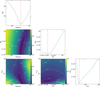 |
Fig. C.1 Maps of χ2 values obtained from the minimization procedure using maximum intensities and spatial separations. The best-fit solution, corresponding to Pth = 3.2 × 10⁶ K cm−3, G0 = 42, and RC = 0.032 pc, is marked by a red circle. Constraints on G0 and RC remain weak, with the χ2 surface appearing relatively flat (bottom center panel), except for very small RC values. For comparison, a model adopting literature values (Pth = 4 × 10⁶ K cm−3, G0 = 100) is shown by a green circle in the G0–Pth panel. |
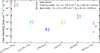 |
Fig. C.2 Observed maximum intensities of various tracers (colored crosses) compared with model predictions (symbols with error bars). Squares show the best-fit model from the minimization described in Appendix C, while circles represent the model obtained in Section 4.4 using literature parameters with G0 = 100. All tracers are well reproduced, except for H2O, for which the models over-predict the observed maximum intensity by about an order of magnitude. The error bars of 40% on models represent geometrical uncertainties and the complexity of the parameter space. |
All Tables
All Figures
|
Fig. 1 (Left panel) SPIRE 350 μm image of the Horsehead PDR. The white circle shows the FWHM SPIRE beam (25.2″). Black circles show the locations at which 557 GHz o-H2O spectra were obtained, with the circle size corresponding to the FWHM HIFI beam (38.1″). (Right panel) Spectra of the 557 GHz o-H2O and CO (2–1) lines across the PDR (black and blue curves, respectively), labeled by the right ascension offsets with respect to the reference position. The CO 2–1 spectra have been scaled down by a factor of 200. The bottom-right panel shows spectra of the ground state o– and p–H2O lines at the central position. |
| In the text | |
|
Fig. 2 Integrated line intensities of atomic and molecular tracers computed over a 9.2–11.8 km s−1 velocity range across the PDR as a function of right ascension offset at Δδ = 0. (Top) [C II], [C I], and H2O (black, blue, and magenta, respectively). (Bottom) CO (2–1), C18O (2–1), CO (4–3), and H2O (black, blue, red, and magenta, respectively). Line intensities have been normalized to their maxima toward the PDR, with the corresponding scaling factors as labeled. The data are shown at the native resolution of the images, with the corresponding FWHM beam sizes marked for each tracer. The size of the squares corresponds approximately to ±1σ H2O observational uncertainties. |
| In the text | |
|
Fig. 3 Same as Figure 2 except that all tracers are convolved to the 38.1″ resolution of the HIFI H2O spectra. |
| In the text | |
|
Fig. 4 Illustration of the geometry of 1D PDR models made with the Meudon PDR code. We show the two-component radiation field composed of a beamed part representing the stellar radiation field and an isotropic part representing the ISRF. This configuration yields the typical chemical stratification, with the ionization front denoting the beginning of the PDR, followed by the dissociation front, or H/H2 transition, and the C+/C/CO transition deeper in the cloud. H2O appears even deeper. |
| In the text | |
|
Fig. 5 Illustration of the geometry of the PDR wrapper. (Left panel) Image of the Horsehead nebula as seen by the Euclid space telescope (Credits: ESA/Euclid/Euclid Consortium/NASA, image processing by J.-C. Cuillandre (CEA Paris-Saclay), G. Anselmi). Notice the reference frame, with the x-axis corresponding to the direction of the lines of sight. We rotate the nebula so that the x–axis points to the right. (Middle panel) Artistic interpretation of the rotation of the Horsehead nebula, generated using OpenAI’s DALL·E model based on the first panel image. (Right panel) Geometry of the wrapping 2D model, with the star radiation field coming from the top, and examples of Meudon PDR model output overplotted as vertical red lines. Each of these lines correspond to a PDR model as represented on Fig. 4. Notice that we use the same model for each position along the cut of the cloud. The multiple lines of sight correspond to different pixels along a vertical 1D cut in the Horsehead nebula. We emphasize that only the lines of sight shown as solid lines are correctly accounted for by the model, as the central section of the nebula outside of the crescent-shaped area is not included in the computations. The geometry is assumed to be circular with a radius of curvature that remains to be determined. |
| In the text | |
|
Fig. 6 Illustration of the wrapper geometry, showing RGB composite maps of carbon-bearing species for different radii of curvature. The color encodes the local abundances as follows: red for ionized carbon (C+), green for neutral atomic carbon (C), and blue for carbon monoxide (CO). Areas where these species coexist appear as color blends (e.g., cyan for C and CO, yellow for C+ and C, white for equal contributions). The left panel shows a curvature radius of RC = 0.05 pc, the middle to RC = 0.2 pc, and the right to RC = 0.5 pc. These maps highlight the local spherical curvature in the plane of the sky, with the observer located at the bottom of each panel and the stellar radiation field entering from the right. Radiative transfer is computed along vertical lines from top to bottom in this configuration. The abundances originate from a single Meudon PDR model (Pth = 4 × 10⁶ K cm−3, G0 = 100). The usual edge-on representation of abundances of this model can be found in Figure 10. |
| In the text | |
|
Fig. 7 A map of χ2 values obtained from the minimization procedure using maximum intensities and spatial separations. The best-fit model, corresponding to Pth = 4.1 × 10⁶ K cm−3, and RC = 0.057 pc, is denoted by the orange circle on the map. The constraint on RC remains weak, with the χ2 surface relatively flat in a wide valley. |
| In the text | |
|
Fig. 8 (Top) Spatial profiles of normalized emission line intensities observed in the Horsehead nebula, compared with predictions from a Meudon PDR model with Pth = 4 × 10⁶ K cm−3 and G0 = 100, wrapped in a locally spherical cloud with a curvature radius RC = 0.05 pc. These conditions correspond to commonly adopted literature values. The left panels show the raw profiles from the wrapping procedure, while the right panels present the same profiles convolved to the native angular resolution of each tracer. In those figures, the radiation field comes from the right. (Bottom) Observed maximum intensities of various tracers (colored crosses) compared to model predictions (circles with error bars). All tracers are well reproduced, except for H2O, where the model overestimates the observed maximum intensity by an order of magnitude. |
| In the text | |
|
Fig. 9 Spatial profiles of normalized emission line intensities observed in the Horsehead nebula, compared to predictions from Meudon PDR model with Pth = 4 × 10⁶ K cm−3 and G0 = 100, wrapped in a locally spherical cloud with curvature radius RC = 0.05 pc. The profiles are convolved to the native angular resolution of the tracer maps. On this figure, the radiation field comes from the right. We observed a significant shift between the observed H2O profile and the model, the latter being much deeper in the cloud. |
| In the text | |
|
Fig. 10 Abundances of key species with respect to hydrogen nuclei (top panel) and gas temperature (bottom panel) profiles of the Horsehead nebula model with Pth = 4 × 10⁶ K cm−3, G0 = 100, computed with the Meudon PDR code (no wrapping or convolution procedure is applied to these profiles). The H/H2 transition can be seen to take place at around AV ~ 0.06 mag, the C+/C/CO transition is at AV ~ 1.7 mag, and the peak of H2O abundance is reached at an AV ~ 3 mag. |
| In the text | |
|
Fig. 11 Two-component, nonlocal radiative transfer models adapted to the physical conditions in the Horsehead. The upper panel shows the o-H2O 557 GHz synthetic line profiles (continuous curves) and observed line profiles (histograms) at the emission peak. The lower panel shows the predicted excitation temperatures of the 110–101 transition. The blue curves represent the model of the dense PDR component alone. The red curves represent the model of the low-density envelope alone, while the black curves represent the two-component model. |
| In the text | |
|
Fig. 12 Same as the lower panel of Fig. 11 but showing the predicted radial o-H2O 110–101 integrated line intensities. The magenta-filled circles represent the observed line intensities across the Horsehead PDR, with the peak position at Δα = +20″. |
| In the text | |
|
Fig. A.1 Horizontal geometry used for the wrapping of Meudon PDR models. The beamed ISRF remains perpendicular to the line of sight. |
| In the text | |
|
Fig. B.1 Two-component, nonlocal non-LTE radiative transfer model of the Horsehead applied to C18O and C+. The horizontal magenta line shows the observed maximum line intensities of the C18O 2–1 (upper panel) and [C II] 158 μm (lower panel) lines (Table 2). |
| In the text | |
|
Fig. C.1 Maps of χ2 values obtained from the minimization procedure using maximum intensities and spatial separations. The best-fit solution, corresponding to Pth = 3.2 × 10⁶ K cm−3, G0 = 42, and RC = 0.032 pc, is marked by a red circle. Constraints on G0 and RC remain weak, with the χ2 surface appearing relatively flat (bottom center panel), except for very small RC values. For comparison, a model adopting literature values (Pth = 4 × 10⁶ K cm−3, G0 = 100) is shown by a green circle in the G0–Pth panel. |
| In the text | |
|
Fig. C.2 Observed maximum intensities of various tracers (colored crosses) compared with model predictions (symbols with error bars). Squares show the best-fit model from the minimization described in Appendix C, while circles represent the model obtained in Section 4.4 using literature parameters with G0 = 100. All tracers are well reproduced, except for H2O, for which the models over-predict the observed maximum intensity by about an order of magnitude. The error bars of 40% on models represent geometrical uncertainties and the complexity of the parameter space. |
| In the text | |
Current usage metrics show cumulative count of Article Views (full-text article views including HTML views, PDF and ePub downloads, according to the available data) and Abstracts Views on Vision4Press platform.
Data correspond to usage on the plateform after 2015. The current usage metrics is available 48-96 hours after online publication and is updated daily on week days.
Initial download of the metrics may take a while.