| Issue |
A&A
Volume 706, February 2026
|
|
|---|---|---|
| Article Number | A198 | |
| Number of page(s) | 16 | |
| Section | Planets, planetary systems, and small bodies | |
| DOI | https://doi.org/10.1051/0004-6361/202556928 | |
| Published online | 13 February 2026 | |
Starlight-driven flared-staircase geometry in radiation hydrodynamic models of protoplanetary disks
1
Max-Planck-Institut für Astronomie,
Königstuhl 17,
69117
Heidelberg,
Germany
2
Fakultät für Physik und Astronomie, Universität Heidelberg,
Im Neuenheimer Feld 226,
69120
Heidelberg,
Germany
3
Ludwig-Maximilians-Universität München, Universitäts-Sternwarte,
Scheinerstraße 1,
81679
München,
Germany
4
Exzellenzcluster ORIGINS,
Boltzmannstr. 2,
85748
Garching,
Germany
★ Corresponding author: This email address is being protected from spambots. You need JavaScript enabled to view it.
Received:
21
August
2025
Accepted:
2
January
2026
Abstract
Context. Protoplanetary disks observed in the millimeter continuum and scattered light show a variety of substructures. While embedded planets are a common explanation, various physical processes in the disk during the early planet formation phase might also trigger these features. One such possibility that has been theorized previously for passive disks is the thermal wave instability or the stellar irradiation instability, where that the flared disk might become unstable as directly illuminated regions puff up and cast shadows behind them. This would manifest as bright and dark rings and as a staircase-like structure in the disk optical surface.
Aims. We provide a realistic radiation hydrodynamic model to test the limits of the thermal wave instability in starlight-heated protoplanetary disks. We make quantitative comparisons to existing results in the literature from simpler linear theory and 1D models to moment-transfer methods to elucidate the importance of correct numerical treatment for this problem.
Methods. We carried out global axisymmetric 2D hydrostatic and dynamic simulations that include radiation transport with frequency-dependent ray-traced irradiation and flux-limited diffusion. We varied the dust-to-gas ratios and surface densities. We also highlight the role of small grains and dust settling with the first radiation hydrostatic dust models to study starlight-driven shadowing.
Results. We found that starlight-driven shadows are most prominent in optically thick, slowly cooling disks, which are shown by our models with high surface densities and dust-to-gas ratios of submicron grains ϵdg = 0.01. We found that thermal waves form and propagate inward in the hydrostatic limit. In contrast, our hydrodynamic models show bumps and shadows within 30 au that converge to a quasi-steady state on several radiative diffusion timescales, which indicates a long-lived staircase structure. Existing thermal pressure bumps might produce and enhance this effect and form secondary structures due to starlight-driven shadowing downstream. Hydrostatic models with self-consistent dust settling instead show a superheated dust irradiation absorption surface with a radially smooth temperature profile without staircases.
Conclusions. We conclude that we can recover thermally induced flared-staircase structures in radiation hydrodynamic simulations of irradiated protoplanetary disks using the flux-limited diffusion method. The shadowing effect is sensitive to the dust content in the disk. We highlight the importance of modeling dust dynamics consistently to explain starlight-driven shadows.
Key words: accretion, accretion disks / hydrodynamics / radiative transfer / protoplanetary disks
© The Authors 2026
 Open Access article, published by EDP Sciences, under the terms of the Creative Commons Attribution License (https://creativecommons.org/licenses/by/4.0), which permits unrestricted use, distribution, and reproduction in any medium, provided the original work is properly cited.
This article is published in open access under the Subscribe to Open model.
Open Access funding provided by Max Planck Society.
1 Introduction
Disk substructures are ubiquitous in modern observations of planet-forming disks at different wavelengths. These include millimeter thermal emission from ground-based instruments such as the Atacama Large Millimeter/submillimeter Array (ALMA, Andrews et al. 2018), scattered-light observations with the Spectro-Polarimetric High-contrast Exoplanet REsearch (SPHERE) instrument on the Very Large Telescope (VLT, Avenhaus et al. 2018; Benisty et al. 2023), and more recently, studies with the James Webb Space Telescope (JWST, Tazaki et al. 2025). Planets within the disk can carve out gaps (Zhang et al. 2018) that explain substructure, of which the planetary gaps in the PDS 70 and WISPIT 2 systems are direct observational constraints (Keppler et al. 2018; Haffert et al. 2019; van Capelleveen et al. 2025; Close et al. 2025). Many physical processes in the disk might also trigger substructures (Bae et al. 2023), such as zonal flows driven by the magneto-rotational instability (MRI, Uribe et al. 2011; Flock et al. 2015), spirals launched by gravitational instability (GI, Kratter & Lodato 2016), gaps and vortices resulting from the vertical shear instability (VSI, Flock et al. 2020), and spirals and rings as a consequence of misaligned inner disks (Zhang & Zhu 2024; Ziampras et al. 2025a). These substructures can invert the local pressure gradient and radially pile up dust in the disk, thereby acting as dust traps (Whipple 1972; Paardekooper & Mellema 2004; Ormel 2026).
The thermal wave instability (or TWI, also known as the irradiation instability or the self-shadowing instability) is one of the mechanisms proposed to explain rings and gaps in disks (Dullemond 2000; Watanabe & Lin 2008; Siebenmorgen & Heymann 2012; Wu & Lithwick 2021; Ueda et al. 2021) through induced pressure variations and subsequent dust concentrations. Historically, this instability was first studied as a consequence of unstable solutions (Dullemond 2000) to the flared-disk model proposed to account for the observed infrared (IR) excess in spectral energy distributions (SEDs) of passive disks around T Tauri stars (Kenyon & Hartmann 1987; Chiang & Goldreich 1997; D’Alessio et al. 1999). This mechanism bring up an interesting possibility that substructures can form at the disk surface without invoking any additional ingredients, solely through starlight-driven shadowing through variations in the irradiation angle onto the surface of a flared disk. Indications of ripples in the flared-disk scattered-light observations of IM Lup with VLT-SPHERE (Avenhaus et al. 2018) are particularly exciting for this scenario.
The mechanism behind this starlight-driven shadowing is outlined as follows (see also Fig. 1 in Ueda et al. 2021, for an illustration): in vertical hydrostatic equilibrium, the balance between gravity and pressure (set by stellar irradiation heating) yields a passive (irradiated) disk with a flared geometry. The outer regions thus absorb substantially more stellar light than in an internally heated conical disk. For optically thick disks, scale-height perturbations might trigger thermal waves that travel inward, which expand regions in the disk and cast shadows behind them. This shows up as bright and dark bands or shadows in temperature or as staircases in the optical surface. They might be referred to in the literature as unstable shadows to distinguish them from the stable shadow cast by the hot inner rim in transition disks (Dullemond et al. 2001) or due to an opacity transition at the snowline (Baillié et al. 2015).
Several methods have been used to study the problem of starlight-driven shadowing in the literature, such as, time-dependent linear theory (Dullemond 2000; Wu & Lithwick 2021), a simplified 1.5 D treatment (i.e., mimicking vertical information with oblique radiation transfer, Watanabe & Lin 2008; Ueda et al. 2021; Okuzumi et al. 2022; Pavlyuchenkov et al. 2022a), and 2.5D (i.e., 2D {R, z} axisymmetric) Monte Carlo radiative transfer models (Siebenmorgen & Heymann 2012; Wu & Lithwick 2021). These models employed either a hydrostatic or a vertically isothermal approximation to the disk (i.e., temperature fluctuations at the atmosphere instantly propagate to the midplane). In the framework of linear analysis in the optically thick disk approximation (Chiang & Goldreich 1997; D’Alessio et al. 1999; Dullemond 2000), models predict that thermal waves form and propagate inward. Watanabe & Lin (2008) found quasi-periodic waves moving inward that decayed at 1 au. Their results also indicated that the disk might reach approximate steady states with bumps and shadows as the mass accretion rate ![Mathematical equation: $\[\dot{M}\]$](/articles/aa/full_html/2026/02/aa56928-25/aa56928-25-eq1.png) increases. The time-dependent analysis by Ueda et al. (2021) with a 1.5D energy equation, however, was focused on models with inwardly propagating waves and found a staircase structure radially outward up to ~100 au for high dust-to-gas mass ratios. Simulations by Wu & Lithwick (2021) with Monte Carlo models and a global two-layer model by Okuzumi et al. (2022) that accounted for radial reprocessing of starlight within the disk also showed inwardly propagating waves.
increases. The time-dependent analysis by Ueda et al. (2021) with a 1.5D energy equation, however, was focused on models with inwardly propagating waves and found a staircase structure radially outward up to ~100 au for high dust-to-gas mass ratios. Simulations by Wu & Lithwick (2021) with Monte Carlo models and a global two-layer model by Okuzumi et al. (2022) that accounted for radial reprocessing of starlight within the disk also showed inwardly propagating waves.
Based on the coupling of radial wave propagation and vertical radiative transfer, however, a full radiation hydrodynamic treatment is necessary to understand the existence and longterm implications of this instability in realistic disks. Radiation transport can be included in hydrodynamic simulations in several ways. These include moment methods such as flux-limited diffusion (FLD Levermore & Pomraning 1981) in the gray (i.e., frequency-integrated) approach (Kley 1989; Kolb et al. 2013), gray FLD coupled with frequency-dependent ray-traced irradiation (Kuiper et al. 2010; Flock et al. 2013), frequency-dependent multigroup FLD (Robinson et al. 2024), M1 moment-transfer method (Melon Fuksman et al. 2021), a three-temperature M1 scheme (Muley et al. 2023), and more complex discrete ordinate methods (Jiang 2021, 2022).
There have been some efforts to model the thermal wave instability using 2.5 D radiation–hydrodynamic simulations in the recent literature. Pavlyuchenkov et al. (2022b) used a diffusion solver for radiation transport, and Melon Fuksman & Klahr (2022) used M1 moment transfer coupled with frequency-dependent irradiation. While these works reported inwardly propagating thermal waves and shadows in the hydrostatic models, both studies concluded that the instability is damped in dynamical simulations. Melon Fuksman & Klahr (2022) attributed this to the inefficiency in transporting thermal perturbations from the atmosphere to the midplane in the disk, as radial advection is more dominant. Kutra et al. (2024) used a simpler radiative forcing method that enforced the vertically isothermal approximation and found staircase structures that did not propagate inward, but settled in the disk for several orbital timescales. Recently, Mori et al. (2025) also reported thermal wave instability-like behavior in their global nonideal magneto-hydrodynamic models, particularly in the model that included the Hall effect and a magnetic field with an anti-aligned polarity.
We aim to provide limits to the thermal wave instability with a realistic radiation hydrodynamic model with frequency-dependent irradiation and cooling via FLD. We relaxed the vertically isothermal assumption of previous models and modeled advection and thermodynamics in 2.5 D self-consistently. While Kutra et al. (2024) also included mass advection in 2.5D with ATHENA++, our models treat radiation transfer more accurately. The ray-traced irradiation + FLD approach also modeled the transition from the optically thick to the thin regime better (Kuiper & Klessen 2013) than Pavlyuchenkov et al. (2022b), which is more suited for optically thick disks. We also explored a higher resolution than they did, and we compared our models with the M1 moment-transfer method (Melon Fuksman & Klahr 2022). Finally, we extended the gas-only disk simulations to include dust settling in the hydrostatic approach. This provided the first results on the effect of dust on starlight-driven shadows and the thermal wave instability.
For clarity, we adopt the following definitions for the words staircase, bump, and shadow: A staircase is a step-like modulation in the irradiation absorption surface as a function of radius, consisting of a heated puffed-up front (a bump) and a colder backside (a shadow). In this context, we note that a bump refers to the locally elevated irradiated region and not to the more traditional temperature or pressure gradient inversion commonly associated with the term. A shadow, in turn, corresponds to the dip in the irradiation flux downstream, which we trace through the midplane temperature decrease of at least 5% relative to the background power law. This is clearly illustrated by the sketch in Fig. 1. In Sect. 2, we outline the physics of our model, the model parameters, and the numerical methods we used. In Sects. 3–5, we show the results from our hydrostatic, dynamical, and dust models. We then discuss the implications of our results in the context of previous work in Sect. 6 and summarize our findings in Sect. 7.
2 Physics, model setup, and numerics
In this section we outline the physics used in our model. We start with the gas dynamics and then describe the radiation method, whose self-consistent treatment is crucial for capturing how the disk responds to thermal perturbations.
2.1 Radiation hydrodynamic equations
We write down the conservative equations for gas dynamics and radiation transport in the gray flux-limited diffusion approximation following Flock et al. (2013). For gas density ρ, velocity u, total energy density Etot, radiation energy density Erad and radiation flux Frad, they read
![Mathematical equation: $\[\frac{\partial \rho}{\partial t}+\nabla \cdot(\rho \boldsymbol{u})=0,\]$](/articles/aa/full_html/2026/02/aa56928-25/aa56928-25-eq2.png) (1a)
(1a)
![Mathematical equation: $\[\frac{\partial(\rho \boldsymbol{u})}{\partial t}+\nabla \cdot(\rho \boldsymbol{u} \otimes \boldsymbol{u}+P \mathbf{I})=-\rho \nabla \Phi_{\star},\]$](/articles/aa/full_html/2026/02/aa56928-25/aa56928-25-eq3.png) (1b)
(1b)
![Mathematical equation: $\[\begin{aligned}\frac{\partial E_{\mathrm{tot}}}{\partial t}+\nabla \cdot & {\left[\left(E_{\mathrm{tot}}+P\right) \boldsymbol{u}\right]=-\rho \boldsymbol{u} \cdot \nabla \Phi_{\star} } \\& -\kappa_{\mathrm{P}} \rho c\left(a_{\mathrm{R}} T^4-E_{\mathrm{rad}}\right)-\nabla \cdot F_{\star}\end{aligned}\]$](/articles/aa/full_html/2026/02/aa56928-25/aa56928-25-eq4.png) (1c)
(1c)
![Mathematical equation: $\[\begin{gathered}\frac{\partial E_{\mathrm{rad}}}{\partial t}+\nabla \cdot \boldsymbol{F}_{\mathrm{rad}}=\kappa_{\mathrm{p}} \rho c\left(a_{\mathrm{R}} T^4-E_{\mathrm{rad}}\right), \\\boldsymbol{F}_{\mathrm{rad}}=-\frac{\lambda c}{\kappa_{\mathrm{R}} \rho} \nabla E_{\mathrm{rad}}.\end{gathered}\]$](/articles/aa/full_html/2026/02/aa56928-25/aa56928-25-eq5.png) (1d)
(1d)
The gravitational potential of the star is given by Φ⋆ = −GM⋆/r where G is the gravitational constant, M⋆ is the mass of the central star, and ![Mathematical equation: $\[r=\sqrt{R^{2}+z^{2}}\]$](/articles/aa/full_html/2026/02/aa56928-25/aa56928-25-eq6.png) is the spherical radius distance to the star. The total energy is a function of kinetic energy and the specific internal energy e with
is the spherical radius distance to the star. The total energy is a function of kinetic energy and the specific internal energy e with ![Mathematical equation: $\[E_{\text {tot }}=\rho e+\frac{1}{2} \rho \boldsymbol{u}^{2}\]$](/articles/aa/full_html/2026/02/aa56928-25/aa56928-25-eq7.png) . The gas pressure is denoted by P, and I is the unit matrix. The temperature-dependent Planck and Rosseland mean opacities are κP and κR respectively, aR is the radiation constant, and c is the speed of light. The set of equations is complete with a closure relation, that is, the ideal gas equation P = (γ −1)ρe with the adiabatic index chosen as γ = 1.42 (Decampli et al. 1978) and the mean molecular weight μ = 2.35. The gas temperature T is given by e = ρcVT, with cV = Rgas/μ(γ − 1) being the specific heat capacity at constant volume, and Rgas the gas constant. The isothermal sound speed is defined as
. The gas pressure is denoted by P, and I is the unit matrix. The temperature-dependent Planck and Rosseland mean opacities are κP and κR respectively, aR is the radiation constant, and c is the speed of light. The set of equations is complete with a closure relation, that is, the ideal gas equation P = (γ −1)ρe with the adiabatic index chosen as γ = 1.42 (Decampli et al. 1978) and the mean molecular weight μ = 2.35. The gas temperature T is given by e = ρcVT, with cV = Rgas/μ(γ − 1) being the specific heat capacity at constant volume, and Rgas the gas constant. The isothermal sound speed is defined as ![Mathematical equation: $\[c_{\mathrm{s}}=\sqrt{P / \rho}\]$](/articles/aa/full_html/2026/02/aa56928-25/aa56928-25-eq8.png) and the gas pressure scale height is given by H = cs/ΩK where
and the gas pressure scale height is given by H = cs/ΩK where ![Mathematical equation: $\[\Omega_{\mathrm{K}}=\sqrt{G M_{\star} / R^{3}}\]$](/articles/aa/full_html/2026/02/aa56928-25/aa56928-25-eq9.png) is the Keplerian angular velocity.
is the Keplerian angular velocity.
The two coupled equations for radiative transfer are given by
![Mathematical equation: $\[\frac{\partial e}{\partial t}=-\kappa_{\mathrm{P}} \rho c\left(a_{\mathrm{R}} T^4-E_{\mathrm{rad}}\right)-\nabla \cdot F_{\star},\]$](/articles/aa/full_html/2026/02/aa56928-25/aa56928-25-eq10.png) (2a)
(2a)
![Mathematical equation: $\[\frac{\partial E_{\mathrm{rad}}}{\partial t}+\nabla \cdot \boldsymbol{F}_{\mathrm{rad}}=\kappa_{\mathrm{P}} \rho c\left(a_{\mathrm{R}} T^4-E_{\mathrm{rad}}\right).\]$](/articles/aa/full_html/2026/02/aa56928-25/aa56928-25-eq11.png) (2b)
(2b)
We write the radiation flux above in terms of the radiation energy density with a flux limiter λ which accounts for the optically thick (λ → 1/3) and thin regimes (Frad → cErad, see also Kolb et al. 2013). We use the flux limiter of Levermore & Pomraning (1981) which is given by ![Mathematical equation: $\[\lambda=\frac{2+X}{6+3 X+X^{2}}\]$](/articles/aa/full_html/2026/02/aa56928-25/aa56928-25-eq12.png) with
with ![Mathematical equation: $\[X=\frac{\left|\nabla E_{\text {rad}}\right|}{\kappa_{\mathrm{R}} \rho E_{\text {rad}}}\]$](/articles/aa/full_html/2026/02/aa56928-25/aa56928-25-eq13.png) .
.
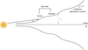 |
Fig. 1 Schematic to illustrate the different terms bump, shadow, and staircase defined in the introduction. The star is denoted by the orange blob, and the stellar rays hit the irradiation absorption surface τ⋆ = 1 at a height zs = z (τ⋆ = 1) from the midplane and a flaring angle φ. |
2.2 Frequency–dependent irradiation
The transition between the optically thick midplane of the disk to the optically thin surface is better captured by including ray-traced irradiation from the star at different frequencies (Kuiper et al. 2010). The frequency–dependent irradiation flux F⋆ from the central star is written in terms of the black body spectrum Bν(T⋆),
![Mathematical equation: $\[F_{\star}(r)=\int_\nu \pi B_\nu\left(T_{\star}\right)\left(\frac{R_{\star}}{r}\right)^2 e^{-\tau_\nu(r)} d \nu,\]$](/articles/aa/full_html/2026/02/aa56928-25/aa56928-25-eq14.png) (3)
(3)
with the optical depth τν defined as an integral over the solid angle Ω and frequency ν (or wavelength λ = c/ν),
![Mathematical equation: $\[\tau_\nu(r)=\int_{R_{\star}}^r \kappa_\nu \rho d r=\tau_{\nu, 0}\left(r_{\mathrm{beg}}\right)+\int_{r_{\mathrm{beg}}}^r \kappa_\nu \rho d r.\]$](/articles/aa/full_html/2026/02/aa56928-25/aa56928-25-eq15.png) (4)
(4)
The optical depth is a function of the frequency-dependent absorption opacity κν and the density ρ. Following Melon Fuksman & Klahr (2022), we use tabulated values for opacities provided by the dust from Krieger & Wolf (2020, 2022). We plot κν, κP, and κR, along with the blackbody function Bλ(T⋆) = c/λ2Bν(T⋆) for T⋆ = 4000 K in Fig. 2. We do not model the hot inner rim of the disk that otherwise casts a shadow, and instead compute an effective optical depth τν,0 from the central star out to the edge rbeg of the disk region of particular interest for our problem, given by
![Mathematical equation: $\[\tau_{\nu, 0}\left(r_{\text {beg }}\right)=\kappa_\nu \rho_{r_{\text {beg }}}\left(r_{\text {beg }}-R_{\star}\right),\]$](/articles/aa/full_html/2026/02/aa56928-25/aa56928-25-eq16.png) (5)
(5)
following a similar prescription from Flock et al. (2013). A more detailed discussion on this initial optical depth profile and how it aligns with our current understanding of the inner disk structure can be found in Sect. 6.6. We then calculate the irradiation flux at each cell center by ray-tracing for different frequency bins.
2.3 Model parameters
For our reference run MFID we model a T Tauri central star, similar to previous models in the literature (e.g., Watanabe & Lin 2008; Ueda et al. 2021; Melon Fuksman & Klahr 2022), with a mass M⋆ = 1 M⊙, radius R⋆ = 2.6 R⊙, effective temperature T⋆ = 4000 K, and luminosity L⋆ = 1.56 L⊙. We implement a surface density power law of Σ(R) = Σ0 (R/1 au)−1, with R being the cylindrical radius. We use Σ0 = 200 g cm−2 for the MFID model, consistent with dust-mass based measurements at 1 au (van Boekel et al. 2017). To explore the effects of higher disk masses, we also consider a model with Σ0 = 2000 g cm−2 (MSIG2000), which is more representative of classical minimum-mass solar nebula models (MMSN, Weidenschilling 1977; Hayashi 1981). While dust mass estimates support the lower surface densities, we explore both models as gas mass estimates still remain poorly constrained. The higher surface density profile matches the one computed using a viscous disk model with a mass accretion rate ![Mathematical equation: $\[\dot{M}\]$](/articles/aa/full_html/2026/02/aa56928-25/aa56928-25-eq17.png) = 10−8 M⊙ yr−1 and viscosity parameter α = 10−3 following Shakura & Sunyaev (1973). This is a commonly used initial condition in disk theoretical studies (including the thermal wave instability, e.g., Watanabe & Lin 2008; Flock et al. 2019; Steiner et al. 2021). However, our models ignore viscous heating (including it would yield a lower Σ in the inner regions, see Fig. 3 of Ziampras et al. 2020), which results in a disk that is marginally more massive in the innermost regions (≲5 au).
= 10−8 M⊙ yr−1 and viscosity parameter α = 10−3 following Shakura & Sunyaev (1973). This is a commonly used initial condition in disk theoretical studies (including the thermal wave instability, e.g., Watanabe & Lin 2008; Flock et al. 2019; Steiner et al. 2021). However, our models ignore viscous heating (including it would yield a lower Σ in the inner regions, see Fig. 3 of Ziampras et al. 2020), which results in a disk that is marginally more massive in the innermost regions (≲5 au).
The initial guess for the temperature is determined by the optically thin solution for a passively irradiated disk (Chiang & Goldreich 1997). We also sample dust-to-gas mass ratios ϵdg = {0.01, 0.001} (models MFID and MD0.001, respectively). A table with the different setups corresponding to the model parameters is given in Table 1. This excludes the hydrostatic dust models for which the parameters are described in detail in Sect. 5. Our models are inviscid and do not account for the effect of accretion heating.
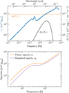 |
Fig. 2 Top panel: frequency-dependent dust absorption opacities (per gram of dust, gdust) from tabulated values (Krieger & Wolf 2020, 2022). The blue points denote 132 frequencies logarithmically sampled in the range ν ∈ [1.5 × 10¹¹, 6 × 10¹⁵] Hz for the computation of irradiation flux in our models. The black line indicates the blackbody function, and the orange line shows the Planck opacity for T⋆ = 4000 K (figure similar to Kuiper et al. 2010). Bottom panel: temperature-dependent Planck and Rosseland mean opacities for the radiation transfer. The local maximum (≈ 250 K) and the subsequent dip in the mean opacities is due to the 10 μm silicate feature. |
2.4 Numerics
We solved the radiation hydrodynamic equations outlined in Eqs. (1) and (2) using the astrophysical finite–volume fluid code PLUTO (Mignone et al. 2007). We use the flux–limited diffusion module outlined in Flock et al. (2013) which uses a Jacobi preconditioned BiCGSTAB solver for the radiation matrix. We perform 2.5 D axisymmetric simulations of gas assuming a constant dust-to-gas mass ratio ϵdg in spherical coordinates (r, θ) with a logarithmic grid in r ∈ [0.41, 95] au and a uniform grid in θ ∈ [π/2–0.32, π/2+0.32]. We use a grid of Nr × Nθ = 1024 × 128 cells, which corresponds to a resolution of ≈6 cps (cells per scale height) in r and ≈7 cps in θ. We use a second-order Runge Kutta (RK2) time integrator, a linear reconstruction scheme, the HLLc Riemann solver (Toro et al. 1994) and a CFL (Courant–Friedrichs–Lewy) value of 0.4.
We implement strict outflow conditions for the radial velocity ur at the radial inner boundary (R < 0.5 au), and use power-law extrapolation for the azimuthal velocity uϕ. The rest of the quantities are set to zero gradient. We also damp the density and velocities at the inner boundary using the de Val-Borro et al. (2006) prescription over a damping timescale of 0.01 inner orbits at R0. For the radiation boundaries, we restrict the radiation energy density at the polar boundaries to a small value ![Mathematical equation: $\[E_{\text {rad }}=a_{R} T_{0}^{4}\]$](/articles/aa/full_html/2026/02/aa56928-25/aa56928-25-eq18.png) , where T0 = 370 ϵdg (R/au)−0.5 K which is about 7% of the optically thin temperature profile for the model MFID (Chiang & Goldreich 1997). Following the prescription in Flock et al. (2016, see their Eq. (19)), we implement a modified gravitational potential in the inner radial boundary to improve numerical stability in the dynamical simulations. In very optical thin regions of the disk we modify the Rosseland mean opacity κR so that κνρrbegΔr > 10−4 is fulfilled. This helps the convergence of the matrix solver without affecting the temperature significantly. Furthermore, we ensure that the radially innermost cell remains optically thin, preventing unphysical heating by the irradiation flux (Flock et al. 2013).
, where T0 = 370 ϵdg (R/au)−0.5 K which is about 7% of the optically thin temperature profile for the model MFID (Chiang & Goldreich 1997). Following the prescription in Flock et al. (2016, see their Eq. (19)), we implement a modified gravitational potential in the inner radial boundary to improve numerical stability in the dynamical simulations. In very optical thin regions of the disk we modify the Rosseland mean opacity κR so that κνρrbegΔr > 10−4 is fulfilled. This helps the convergence of the matrix solver without affecting the temperature significantly. Furthermore, we ensure that the radially innermost cell remains optically thin, preventing unphysical heating by the irradiation flux (Flock et al. 2013).
Parameters for the different hydrostatic and dynamic runs.
2.5 Iterative solver for hydrostatic models
Using the iterative method described in Flock et al. (2013) to compute solutions for irradiated disks in radiative hydrostatic equilibrium, we first run hydrostatic models with the parameters described above. Given an initial density profile ρ(r, θ), this solver iterates between each FLD step given by Eq. (2) over a typical radiative diffusion timescale of ~106 s (for typical solar parameters, see Eq. (C.1)). The extended runtimes with successive diffusion steps reaching up to 108 s in later iterations ensure thermal equilibrium, with temperatures reaching a converged state. Once the radiation solver converges, new densities (and azimuthal velocities) are computed by integrating the hydrostatic equations
![Mathematical equation: $\[\frac{\partial P}{\partial r}=-\rho \frac{\partial \Phi_{\star}}{\partial r}+\frac{\rho u_\phi^2}{r},\]$](/articles/aa/full_html/2026/02/aa56928-25/aa56928-25-eq19.png) (6a)
(6a)
![Mathematical equation: $\[\frac{1}{r} \frac{\partial P}{\partial \theta}=\cot \theta \frac{\rho u_\phi^2}{r},\]$](/articles/aa/full_html/2026/02/aa56928-25/aa56928-25-eq20.png) (6b)
using a second-order Runge–Kutta integrator. The iterative process is continued until a converged density state is reached. The computed profiles are then used as initial conditions for the hydrodynamic simulations. While disk hydrostatics are more correctly treated in cylindrical coordinates (see, e.g., codes like cuDisc, Robinson et al. 2024), our approach works well and has been robustly tested and used for various problems (for validation tests, see Appendix B of Flock et al. 2013).
(6b)
using a second-order Runge–Kutta integrator. The iterative process is continued until a converged density state is reached. The computed profiles are then used as initial conditions for the hydrodynamic simulations. While disk hydrostatics are more correctly treated in cylindrical coordinates (see, e.g., codes like cuDisc, Robinson et al. 2024), our approach works well and has been robustly tested and used for various problems (for validation tests, see Appendix B of Flock et al. 2013).
Previous models of the thermal wave instability suggest that unstable shadows form and propagate inward in such a hydrostatic iterative treatment (Ueda et al. 2021; Okuzumi et al. 2022). Our models further include vertical and radial radiative transfer, relaxing the commonly used isothermal approximation. We start by describing these hydrostatic models, followed by the hydrodynamic simulations in the following sections.
3 Results I: Fiducial model MFID
We first outline results from our fiducial model MFID, for which the model parameters are listed in Table 1. This corresponds to a high dust-to-gas ratio case of ϵdg = 0.01. Such a value represents the early times of disk evolution, where most of the dust material is still in the form of small (≤10 μm) grains. For reference, a total dust-to-gas mass ratio ϵtot = 0.01 for all sizes and MRN dust distribution (Mathis et al. 1977), and a dust-to-gas ratio in small grains ϵdg of 0.01, 0.001 and 0.0001 would yield maximum grain sizes of amax of 0.25 μm, 19 μm and 1.8 mm, respectively (see also Melon Fuksman et al. 2024). At later stages, dust grains grow, settle to the midplane, and small grains become depleted in the disk (Birnstiel et al. 2010; Testi et al. 2014). While ϵdg = 0.01 may be on the higher end for a T Tauri disk, we adopt this value as our fiducial case in order to optimize the conditions under which staircase structures are most likely to develop.
3.1 Hydrostatic model
We see the emergence of alternating bright and dark regions in the disk with thermal waves forming and propagating inward, consistent with the expectations from hydrostatic models in the literature (Watanabe & Lin 2008; Ueda et al. 2021; Pavlyuchenkov et al. 2022a). This is clearly depicted by the midplane temperature profiles plotted for different iteration times in Fig. 3 and also the 2D snapshot of temperature and irradiation heating rate −∇ · F⋆ at the end of the hydrostatic run in Fig. 4.
From Fig. 3, we see that as the disk tries to find a hydrostatic solution, a thermal wave forms and travels inward, and two form after i = 15 iterations that also propagate inward. The perturbations in temperature deviate from the background power law by up to 30%.
We plot the 2D snapshots at the last iteration (i = 30) in Fig. 4. To get a complete picture of where in the disk radiation is emitted and absorbed, we plot different optical depth surfaces, that is, τν = 1 profiles corresponding to the starlight at different frequencies τν and the emission of the disk itself τdisk, defined by
![Mathematical equation: $\[\tau_\nu=\int_{R_{\star}}^r \kappa_\nu \rho d r, \quad \tau_{\mathrm{disk}}=\int_{\theta=\pi / 2}^\theta \kappa_\nu \rho r d \theta.\]$](/articles/aa/full_html/2026/02/aa56928-25/aa56928-25-eq21.png) (7)
(7)
These surfaces exhibit a clear staircase pattern in contrast to the typical smooth flared-disk power-law solution. Nevertheless, it is important to investigate the existence of such a pattern in hydrodynamic simulations to assess their stability. This is discussed in the following section. The red line in Fig. 4 indicates the optical depth to the disk’s own emission τdisk = 1, showing that the disk is optically thick up to R ~ 50 au.
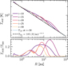 |
Fig. 3 Top: time evolution of the temperature profile at the disk midplane for iterations i = [10, 15, 20, 25, 30]. The profiles indicate that thermal waves form and travel inward with time. There are two bump and shadow pairs at the end of the hydrostatic run for model MFID. The dotted blue line is the radiation temperature at i = 30 and the dashed black line indicates the background power law fit for the midplane Tlaw = 185 (R/au)−0.5. Bottom: deviation of the temperature profile from the background power law. |
3.2 Hydrodynamics
With initial conditions from the previously described hydrostatic model, we introduce dynamics, allowing the system to evolve over time. Plotted in Fig. 5 (top panel) are the profiles of the temperature and the irradiation source term at t = 500 inner orbits or 131.3 yrs. We do not find inwardly propagating waves. Instead, among the bumps in temperature that we started out with in the hydrostatic case, the innermost bump grows in amplitude, and as a result of this bump, the region behind it is shadowed, giving rise to the second one. After about 400 inner orbits, we see that this staircase structure reaches a quasi-steady state that remains stable for several hundreds of orbits. This is clearer in the top panel of Fig. 6, where we plot radial profiles of the midplane temperature normalized to the background power law for different times.
3.2.1 The inner bump
The innermost bump has slightly grown, and shifted inward compared to its radial location in the static models. There are two factors to consider while interpreting this first bump as a consequence of the thermal wave instability. First, its location between 1–2 au, which corresponds to a temperature of ≈ 250 K, coincides with the 10 μm silicate transition1 in the temperature-dependent opacities (see the bottom panel of Fig. 2). This is further indicated by a solid black line in Fig. 5, and the first dashed line in the time evolution plot in Fig. 6. Regions in the disk with opacity transitions can locally change the heating rate, and a strong enough transition could also flatten the pressure gradient causing bumps (Garaud & Lin 2007). While this may not be enough for the formation of this inner bump, it may have an influence. Second, the inner disk is modeled with an effective optical depth profile τν,0, which can affect the first bump through a nonuniform heating rate. In our simulations, we do find a slight enhancement in the irradiation power inward of 1 au (see Fig. D.1) with the prescription of τν,0. A more detailed discussion on this is included in Appendix D.
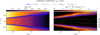 |
Fig. 4 2D profiles of temperature and the irradiation heating term for the hydrostatic model at i = 30 iterations. The orange line refers to the τ⋆ = 1 profile for the stellar radiation using the Planck mean opacity. Blue lines refer to τν = 1 profiles for for different frequencies ν (same as in Fig. 2), with the line opacity weighted by Bν at that frequency. (see also Fig. 7 in Melon Fuksman & Klahr 2022). The red line indicates the τdisk = 1 profile for the disk’s radiation using κP(T). The green lines indicate the midplane gas scale height of the disk. |
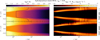 |
Fig. 5 2D profiles of temperature and the irradiation heating term for the hydrodynamic model at t = 500 orbits (top) and t = 10 000 orbits (bottom). The solid black line denotes the temperature corresponding to the opacity transition in Fig. 2. |
3.2.2 Secondary structure around a bump
Regardless of the origin of the first bump, we would like to highlight that the key consequence of this inner bump is that it casts a shadow behind, driving a second one. This second bump is a natural consequence of the first, driven by starlight-driven shadowing. This behavior is unlike that expected by the “thermal wave instability” discussed in Wu & Lithwick (2021) and Ueda et al. (2021), where the staircase pattern propagates inward. Instead, the disk seems to relax to a quasi-steady state characterized by bumps and shadows formed sequentially from the inside out. Forming secondary structure around existing bumps creates interesting implications for disk studies focused on pressure traps (see Sect. 6.7 for a discussion on snowlines).
We plot the radial temperature gradient in the bottom panel of Fig. 6. The bumps and shadows have a clear imprint with modulations of the radial temperature profile. However, neither the first bump and shadow pair nor the subsequent ones in the MFID model produce local extrema (dTmid/dR = 0). The profile remains radially monotonic, albeit with a varying slope.
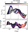 |
Fig. 6 Top: time evolution of the temperature profile at the disk midplane against the background power law. The dashed lines (the first corresponds to the opacity transition) indicate the final locations of the temperature bumps. Bottom: time evolution of the radial temperature gradient indicating a less steep profile at the shadow locations and no sign flip. |
3.3 Long-term evolution of the staircase structure
We run the fiducial model MFID for a long time, the second panel of Fig. 5 shows the 2D profiles after t = 10 000 inner orbits or 2625.3 yr. We see that the two bump and shadow pairs remain in the disk after several thousands of years. This brings up the interesting possibility that they could correspond to long-lived substructure in the disk. Both panels showing temperature in Fig. 5 show hot regions in the upper layers of the inner disk, owing to numerical artifacts that arise due to a combination of strong shocks at very low-density regions and some compressional heating due to the modified gravitational potential (seen also in other works like Melon Fuksman & Klahr 2022; Cecil & Flock 2024).
Our results clearly show that starlight-driven staircases are strongly affected by the hydrodynamics in the disk and also show that the predictions from linear theory and hydrostatic models do not fully come true. Our results for the ϵdg = 0.01 MFID model are different from such predictions where inwardly propagating thermal waves were seen (Wu & Lithwick 2021; Ueda et al. 2021; Pavlyuchenkov et al. 2022a). This is also different from the dynamical models of Melon Fuksman & Klahr (2022), who found that the thermal waves completely damp away, although our setups have a different treatment of the inner disk profile. We show that in the dynamical case, while thermal waves do not propagate inward, they grow and reach a quasi-steady state. While Kutra et al. (2024) hint toward a similar theory of staircases settling in the disk, there are clear differences in the physics we model. We make comparisons to previous works in detail in Sect. 6.
4 Results II: Changing the dust content
We explore the two models MD0.001 and MSIG2000 with lower dust-to-gas ratios of ϵdg = 0.001 and a higher surface density Σ0 = 2000 g/cm2 respectively. Both of these vary the dust content in the disk, which controls the efficiency of radiation transport and hence affects the thermal structure of the disk. The growth rate of the instability, predicted by Ueda et al. (2021), Wu & Lithwick (2021) depends on the height at which the irradiation is absorbed on the surface of the disk. Disks with a higher dust opacity, be it due to a higher ϵdg or gas mass, achieve this. Previous work also verified that for lower dust content, the TWI was suppressed (Ueda et al. 2021; Melon Fuksman & Klahr 2022).
4.1 Low dust-to-gas ratio model MD0.001
In this section we outline our results from our hydrostatic and dynamical models for the low dust-to-gas ratio case of ϵdg = 0.001. As outlined above, these values are more typical to the dust content observed in later stages (i.e., Class II protoplanetary disks Rilinger & Espaillat 2021; Birnstiel 2024). Figure 7 shows the temperature and the irradiation source term after 30 iterations for the hydrostatic model (top) and the hydrodynamic model (bottom) after t = 500 orbits. We do not see any temperature bumps or shadows forming in the hydrostatic model, but recover an inner bump in the dynamic model.
While studies in the literature point toward the TWI being suppressed for very low dust-to-gas mass ratios ϵdg ⪅ 10−4 (Ueda et al. 2021), we do not recover any secondary shadowing already for the ϵdg = 0.001 model. The combined effect of the reduced dust content and a lower radiation boundary (see T0 in Sect. 2.4) could enhance the cooling efficiency of the disk in the outer parts, affecting the formation of staircases. An outline of the cooling timescales in the disk can be found in Appendix C. We speculate that the smaller amplitude of the shadowing with the FLD method might also affect this limit. We discuss this further in Sect. 6.5.
4.2 High surface density model MSIG2000
We now present the results for the model with a surface density of Σ0 = 2000 g/cm2 and a dust-to-gas ratio of ϵdg = 0.01, motivated in Sect. 2.3. A higher surface density not only implies a higher dust content in the disk, with 10 times the amount of dust at a certain radius compared to the fiducial model but also a longer cooling timescale (in the hydrodynamic case the diffusion-regulated cooling timescale scales with Σ2ϵdg; see also Eq. (C.1)). Such a disk would be overall more optically thick than the MFID model, which would have an effect on the temperature structure.
Figure 8 shows the temperature and the irradiation heating term for the hydrostatic and dynamical MSIG2000 models. We see three temperature bumps at the end of the 30 hydrostatic iterations, all within 10 au of the disk. The time evolution of the staircase structure is clearer in Fig. 9, showing how the system readjusts from this static initial condition with three TWI bumps. In the hydrodynamic model, the inner bump continues to grow, altering the structure downstream: the staircases shift inward, and the first bump eventually grows sufficiently to merge with the second. The thermal response time for the disk is 100 times slower than the MFID model, and after about 7000 inner orbits, we see a final state with two bumps (see also the bottom panel of Fig. 8, where the final state is plotted at 12 000 inner orbits). On more careful observation, we can also spot a smaller bump at ~20 au in the disk, with a relative temperature difference of 10%, less noticeable in the 2D profiles (Fig. 8) compared to the more prominent ones (see Sect. 6.5 for a discussion on the amplitude of the bumps in our models). The profiles of the radial temperature gradient in the bottom panel of Fig. 9 show that the innermost bump in the hydrodynamic model causes a temperature gradient inversion i.e., a local maximum in the profile, something that was absent in the fiducial MFID model. The bumps downstream to it are more comparable, with the shadowing causing deviations in the slope of the temperature profile.
Overall, it is clear that the dust content in the disk has a significant effect on the staircase structure: a higher dust content correlates not only to more bumps that are more pronounced, but also show signs of inward motion. This hints at more favorable conditions for the staircase structure in opaque disks, further enhanced by a driving inner bump.
Interestingly, our MSIG2000 model shows inwardly moving waves similar to the predictions of the TWI, until it reaches a steady state after long-term evolution. This behavior could imply that optically thick disks provide more favorable conditions for the TWI itself, but identifying these conditions is beyond the scope of this work.
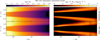 |
Fig. 7 2D profiles of temperature and the irradiation source term for the MD0.001 hydrostatic+dynamic model with ϵdg = 0.001. Top panel: hydrostatic model after t = 30 iterations does not show any staircase structure. Bottom panel: hydrodynamic model after t = 500 orbits shows the innermost bump. |
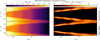 |
Fig. 8 2D profiles of temperature and the irradiation source term for the high surface density MSIG2000 hydrostatic+dynamic model. The hydrostatic run shows three prominent bumps (top), hydrodynamic run shows two bumps (bottom). Midplane temperature reached equilibrium after several radiative diffusion timescales, and hence the longer run time of t ≈ 12 000 orbits. |
5 Results III: Adding dust settling
With the dust content controlling radiation transport in the bulk of the disk via its opacity, modeling dust consistently is crucial to correctly capturing the shape of the thermal surface of the disk, as the latter determines the irradiation absorption surface. Dust settles at different heights and interacts with the gas through drag forces. In almost all previous models studying the thermal wave instability (including the results in our previous sections), there is an inherent assumption that the dust is perfectly coupled to the gas, and that the dust content scales with the gas mass through a constant dust-to-gas ratio. We present the first physically motivated hydrostatic model with dust by introducing a dust scale height within the hydrostatic radiation solver in PLUTO (see Sect. 2.5). In the Epstein regime, the dust–gas drag force depends on the Stokes number St = tstopΩK, which describes how well dust is coupled to the gas. Given a dust grain size of a and a dust density ρd, the stopping time tstop is defined as
![Mathematical equation: $\[t_{\text {stop }}=\frac{\rho_{\mathrm{d}} a}{\rho \boldsymbol{v}_{\text {th }}},\]$](/articles/aa/full_html/2026/02/aa56928-25/aa56928-25-eq22.png) (8)
(8)
where ![Mathematical equation: $\[\boldsymbol{v}_{\text {th }}=\sqrt{8 / \pi} c_{\mathrm{s}}\]$](/articles/aa/full_html/2026/02/aa56928-25/aa56928-25-eq23.png) is the mean thermal velocity (Birnstiel 2024). The vertical profile for the dust can be determined by the settling–diffusion equilibrium. A simple model usually imposes a Gaussian profile for the dust similar to the gas, although now with the dispersion being the dust scale height Hd (e.g., observations of IM Lup in Pinte et al. 2008). A more general approach involves modeling dust turbulence as a diffusive process (Dubrulle et al. 1995; Dullemond & Dominik 2004; Mulders & Dominik 2012). A steady state solution for vertical settling and turbulent diffusion can be written in terms of the diffusion coefficient D which quantifies diffusivity. For the simplest case, we utilize the solution assuming D = αdcsH, where αd is a dimensionless diffusion parameter. The dust density structure is then given by Fromang & Nelson (2009)
is the mean thermal velocity (Birnstiel 2024). The vertical profile for the dust can be determined by the settling–diffusion equilibrium. A simple model usually imposes a Gaussian profile for the dust similar to the gas, although now with the dispersion being the dust scale height Hd (e.g., observations of IM Lup in Pinte et al. 2008). A more general approach involves modeling dust turbulence as a diffusive process (Dubrulle et al. 1995; Dullemond & Dominik 2004; Mulders & Dominik 2012). A steady state solution for vertical settling and turbulent diffusion can be written in terms of the diffusion coefficient D which quantifies diffusivity. For the simplest case, we utilize the solution assuming D = αdcsH, where αd is a dimensionless diffusion parameter. The dust density structure is then given by Fromang & Nelson (2009)
![Mathematical equation: $\[\rho_{\mathrm{d}}=\rho_{\mathrm{d}, ~\text {mid}} ~\exp \left[-\frac{\mathrm{St}_{\mathrm{mid}}}{\alpha_{\mathrm{d}}}\left(\exp \left(\frac{z^2}{2 H^2}\right)-1\right)-\frac{z^2}{2 H^2}\right].\]$](/articles/aa/full_html/2026/02/aa56928-25/aa56928-25-eq24.png) (9)
(9)
We compute the dust density at the midplane from this formula at the end of every hydrostatic iteration once the new temperatures and gas densities are determined. In our models, we consider a fixed grain size of a = 10 μm and dust density ρd = 3 g cm−3.
Figure 10 shows 2D profiles of temperature and the irradiation source term for the dust models, for different diffusion parameters αD ∈ [0.0001, 0.001, 0.01]. We see a superheated dust layer and a very sharp irradiation surface for all cases, with dust settling more for a lower αD (Zsom et al. 2011). For a given grain size, the dust–gas coupling is stronger where the gas density is higher. While the dust and gas are well coupled in the midplane, there is a sharp transition layer at the height where the dust is no longer well-coupled to the gas, and the dust density drops rapidly. Since the dust layer dictates the irradiation surface, this results in sharp layers where the majority of the irradiation from the star is absorbed (Chiang & Goldreich 1997). The height at which the radiation is absorbed is thus substantially closer to the midplane, an effect usually neglected in previous work on this topic. This affects the flaring angle of the disk, and hence the temperature structure. We see that staircases are not formed in any of these hydrostatic models with the dust scale height included.
While these models are already a first step to evolve dust in the disk, this iterative static settling–diffusion approach breaks down at a few gas scale heights. Our radiation transfer method accounts for small grain opacities through the precomputed opacity tables based on a grain size distribution, but the assumption of a constant 10 μm mass-carrying component, which would experience moderate settling is a simplification (see Sect. 5 for a more detailed discussion on caveats of the existing dust models). To fully consistently model the transition of coupled-to-decoupled dust grains, we would have to model dust–gas interaction with drag and turbulent diffusion, along with the opacity feedback on radiation transport. We note that including this could affect the preliminary results with dust discussed in this section. Our future work will focus on this aspect in more detail, modeling dust as a pressureless fluid with the PLUTO code (outlined in Ziampras et al. 2025b).
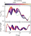 |
Fig. 9 Top: long-term time evolution of the midplane temperature deviation from the background power law for the dynamical model MSIG2000. After about t = 700 orbits, we see that the first and the second bump merge together. We can also spot an additional bump at ≈20 au. The dashed green line corresponds to the final state of the MFID model in Fig. 6, for comparison. Bottom: the evolution of the radial temperature gradient in time similar to Fig. 6. Here, we see that the innermost bump is a local maximum, producing a temperature gradient inversion, while the other two shadows produce slope changes in the profile. |
6 Discussion
In this section, we discuss some additional aspects of our models, such as the physical implications of the shadows and their observability, the effect of the initial optical depth profile, the dust scale height, and the cooling timescales, which might be important for the long-term evolution of shadows in the disk. We will also draw some qualitative comparisons to previous work on the thermal wave instability to the linear theory and hydrostatic models of Wu & Lithwick (2021), Ueda et al. (2021), and the hydrodynamic models of Pavlyuchenkov et al. (2022b), Melon Fuksman & Klahr (2022), and Kutra et al. (2024). Finally, we highlight some caveats of our work and future directions.
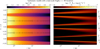 |
Fig. 10 2D profiles of temperature and the irradiation heating term for the hydrostatic model with a dust tracer at i = 30 iterations for diffusion coefficients αD ∈ [0.0001, 0.001, 0.01]. We see a very sharp irradiation surface but there are no staircases formed in any of these models. |
6.1 Physical implications of the bumps and shadows
To understand if the staircase structure we see in our radiation hydrodynamic simulations can produce observable features, in addition to the relative midplane temperature profiles and the temperature gradients plotted in Figs. 6 and 9, we provide further analysis here. The first two panels of Fig. 11 show the radial profiles of the luminosity factor φ = sin α, where α is the flaring (grazing) angle and the height of the irradiation surface normalized to the local radius zs/R where zs = z (τ⋆ = 1). The flaring angle is the angle at which stellar rays hit the surface of the disk defined similar to the classical approach of Chiang & Goldreich (1997) and Dullemond (2000), where α = arctan (dzs/dR) – arctan (zs/R) and the irradiation factor φ is the fraction of luminosity intercepted by the disk surface, essentially approximating Eq. (3) as
![Mathematical equation: $\[F_{\star} \approx \phi \frac{L_{\star}}{4 \pi r^2}.\]$](/articles/aa/full_html/2026/02/aa56928-25/aa56928-25-eq25.png) (10)
(10)
For small angles (i.e., razor-thin disks), φ ≃ α. We use the above mentioned quantities to trace whether the bump and shadow pairs produced in our models can affect the optical or near-infrared (NIR) intensities producing observable signatures. We see that φ decreases downstream of the bumps, blocking stellar rays to efficiently reach the shadows. This is also reflected by the nonuniform profiles of zs/R, deviating from a smooth power-law profile. This provides evidence that the optical/NIR intensities are indeed reduced in the shadowed regions, but to also illustrate this further we provide synthetic scattered-light images in the H Band (VLT-SPHERE) with RADMC-3D (Dullemond et al. 2012) in Appendix. B showing that our models produce bright rings and subsequent dark shadows. We also plot the midplane pressure gradient for our models in the bottom panel of Fig. 11 to understand the implications of the shadows/bumps in our models in the mm continuum. We do not see the inversion of the pressure gradient (i.e., dust traps, Whipple 1972; Paardekooper & Mellema 2004) for any of our models, but we see deviations in the pressure gradient at the shadow locations. This implies that while the staircase structure due to the starlight-shadowing mechanism is not strong enough to trap dust, they could act as dust traffic jams that could slow down dust grain drift, and also act as seeds for secondary dust accumulation mechanisms (Jiang & Ormel 2021). We highlight that the self-consistent modeling of dust–gas dynamics coupled with radiation transfer is required for more accurate constraints on observable signatures of shadows, which is why providing state-of-the-art synthetic observations both in NIR and the mm continuum is not the focus of this work.
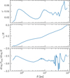 |
Fig. 11 Top: radial profile of the luminosity factor φ at the irradiation absorption surface showing a decreased incidence of stellar rays in the shadowed regions. Middle: radial profiles of the surface aspect ratio h at the τ⋆ = 1 surface. We see that the profiles deviate from a smooth power-law. Bottom: midplane radial pressure gradient shows deviations in the pressure profile. We note the flaring angle φ and the midplane pressure gradient d log Pmid/d log R are smoothed with a rolling average over 20 cells to eliminate noise. |
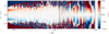 |
Fig. 12 Vertical velocity profiles of the disk at t = 10 000 orbits normalized to the sound speed. We see the development of the VSI modes in the outer disk. The dashed line indicates the location where VSI is expected according to the Lin & Youdin (2015) criterion. |
6.2 Vertical velocity profiles of the long-term evolved models
As mentioned in Sect. 3.3, we ran the fiducial model MFID for several radiative diffusion timescales and saw long-lived staircases. Figure 12 shows the vertical velocity profile of the disk at t = 10 000 orbits. In the outer disk (≳10 au), we see characteristic vertical motions extending from the top and bottom surfaces to the midplane (the so called finger modes) of the vertical shear instability (VSI, Nelson et al. 2013; Pfeil & Klahr 2019). We also see some fully developed (corrugation) modes extending throughout the whole disk. The VSI is a hydrodynamic instability that could occur in outer protoplanetary disks where the cooling timescale is short, and can generate turbulence levels that match the ones observed in disks (Dullemond et al. 2022; Villenave et al. 2025). Although typical studies of the VSI require a higher resolution (~16 cps) to capture saturated states, and even higher (~50 cps) for accurate growth rates (Flores-Rivera et al. 2020), we can still resolve the characteristic motions for grid sizes used in this study (Ziampras et al. 2023). A more detailed calculation of the cooling timescales in our model can be found in Appendix C. The VSI is expected to mix small grains in the disk efficiently (Dullemond et al. 2022). A combination of a VSI-active outer disk and a vertically settled dust layer in the inner regions could further result in a sharp radial transition of the height of the dust layer, affecting or even promoting structure due to starlight-driven shadowing. This can only captured by models with self-consistent dust dynamics.
6.3 Hydrodynamic modeling changes the picture: Comparisons to linear theory and hydrostatic studies
Within the framework of linear analysis in the optically thick disk approximation, D’Alessio et al. (1999) showed that the disk is stable to temperature perturbations for very long cooling times (e.g., in the inner disk) and Dullemond (2000) found unstable thermal waves for short cooling times (e.g., in the outer disk). We find that temperature bumps and shadows are most likely between 1–30 au, corresponding to intermediate-to-long cooling times (similar to the findings of Wu & Lithwick 2021). Time-dependent analysis by Watanabe & Lin (2008) and Ueda et al. (2021) found shadows radially outward up to ~100 au for dust-to-gas mass ratios up to ϵdg = 0.001. While both linear theory (Dullemond 2000), and hydrostatic models (Ueda et al. 2021; Wu & Lithwick 2021; Okuzumi et al. 2022) found inwardly propagating waves, we find temperature bumps that grow and reach a quasi-steady configuration in our models, similar to models of Watanabe & Lin (2008) with stabilized shadows for high mass accretion rates ![Mathematical equation: $\[\dot{M}\]$](/articles/aa/full_html/2026/02/aa56928-25/aa56928-25-eq26.png) . While we see some inward motion of bumps in the MSIG2000 model, they also reach a quasi-steady state after a few thousand orbits.
. While we see some inward motion of bumps in the MSIG2000 model, they also reach a quasi-steady state after a few thousand orbits.
We show that linear theory and vertically isothermal hydrostatic models do not accurately reflect the conditions in the disk. Consistent radial and vertical transport of radiation and advection indicate a more quasi-setady picture than a disk susceptible to a thermal wave or a self-shadowing instability. While this nonlinear quasi-steady state remains to be fully constrained, the natural formation of long-lived shadows in the disk is an interesting explanation for the origin of some of the ubiquitously observed substructures in protoplanetary disks.
6.4 Comparisons to existing hydrodynamic models
Kutra et al. (2024) performed hydrodynamic simulations with a simplified cooling model, where they relaxed the local temperature of the disk toward a forcing temperature calculated based on a vertical integration of the irradiation source term, over the thermal relaxation timescale. This restricts their model effectively to a vertically isothermal approximation, implying changes in the temperature at the surface are propagated downward almost instantaneously likely favoring the formation of staircases (Melon Fuksman & Klahr 2022). They perform hydrodynamic simulations with gray irradiation, constant opacities for the dust, and find staircases forming in the disk that stall.
While our hydrodynamic models with frequency-dependent irradiation and the flux-limited diffusion method also predict a similar quasi-steady state, it is important to note key differences in physics. Solving 2D axisymmetric hydrodynamics with a simplified cooling model (one that is effectively vertically isothermal) constrains thermal evolution to being a purely radial process. Heating and cooling due to vertical compression, expansion, or radiative diffusion is affected by the imposed vertical temperature profile to which the system is forced to relax. We believe that this can cause unphysical propagation or even amplification of temperature perturbations, exaggerating the staircase structure (to similar amplitudes like in 1.5D simulations, e.g., Ueda et al. 2021). Moreover, the thermal relaxation timescale they use is vertically constant throughout the disk (see Fig. 1 of Kutra et al. 2024), not capturing the transitions in optical depth from the disk surface to the midplane nor vertical heat diffusion. For context, their model matches closely to our MSIG2000 model, but while their midplane reaches equilibrium after a few hundred orbits, the same takes several thousand orbits in our model.
Pavlyuchenkov et al. (2022b) also performed hydrodynamic simulations with a diffusion method, one that handles radiation transport in the optically thick regime accurately, but is artifically too diffusive in the optically thin and transition regions. This results in excessively rapid cooling near the optically thin disk atmosphere, where dust densities and therefore cooling rates, that are proportional to ρϵdgκP are extremely low. Our model uses a flux limiter to capture both regimes, and also includes frequency-dependent ray tracing which improves the treatment of the radiation field (Kuiper & Klessen 2013). Their initial conditions differ from ours and more closely resemble a disk around a Herbig star with a luminosity of L = 5 L⊙. They include the inner rim, which when heated by such a bright star, puffs up and casts a wide shadow radially that extends outward into the optically thin region, thereby suppressing other bumps in the domain. Kutra et al. (2024) showed that this shadow extended to about 20 au, and recovered the temperature bumps as the shadow was smaller when they used stellar properties similar to our work. They use a sparse grid resolution (especially in the vertical direction), which might have prevented them from capturing the irradiation surface accurately, inhibiting the formation of shadows in the disk.
Melon Fuksman & Klahr (2022) used the M1 closure for radiation transport along with frequency-dependent irradiation. While in hydrostatic models we see that the M1 method produces temperature bumps that are more pronounced in amplitude than the ones we see with FLD, they always found that the thermal waves damp away when including hydrodynamics. This is in contrast to our findings, with the two shadows stabilizing for several hundreds of orbits in our simulations. We nevertheless compare our radial midplane temperature profiles and find that they match quite well (see Appendix A). Our prescriptions of the inner disk and the initial optical depth differ, where we adopt a simpler prescription following Eq. (5) and Flock et al. (2013). We discuss the implications of using different initial optical depth profiles in Sect. 6.6 and the differences between our models in Appendix D.
The differences in the radiation methods among all of these existing hydrodynamic studies make it difficult to establish direct comparisons. This acts as motivation for future studies to compare the different methods in a systematic way to constrain the reliability of the irradiated disk studies. More complicated methods like the half-moment (HM) method (Melon Fuksman et al. 2025) and the discrete ordinate methods Jiang (2021) could help resolve the discrepancy.
6.5 The amplitude of the bumps with FLD
We see that the largest amplitude of the bumps (with the inner bump being the strongest) is about 40% relative to the background power law. The shadows resolved with our FLD model are less steep compared to those resolved with other radiation methods. In comparison, bumps in the M1 hydrostatic models of Melon Fuksman & Klahr (2022) showed amplitudes of order 50–60% (see Fig. A.1). The models of Kutra et al. (2024) show bumps that stand out by a factor of 2, more consistent with a 1D thermodynamic approach. With FLD, we also see that the bumps are not strong enough for a temperature gradient inversion (except for the inner bump in the MSIG2000 model) as opposed to the above mentioned methods, where they are locations of local extrema. These differences are expected with different radiation methods, details of are explored in code comparison works like Menon et al. (2022) and Thomas & Pfrommer (2022).
6.6 The inner disk structure and the initial optical depth
The structure and evolution of the inner rim of a protoplanetary disk is still an active field of research. The disk at the magnetospheric radius, studied by previous works like Dullemond et al. (2001) and in radiation hydrodynamical models like Flock et al. (2019); Chrenko et al. (2024); Flock et al. (2025), is expected to feature a hot, puffed-up inner rim which casts a shadow upon the outer disk. Hence, there is still uncertainty about choosing the exact inner disk profile and whether the prescription for the optical depth of the inner disk τν,0 (see Eq. (5)) is realistic. Our prescription of the initial optical depth is similar to the one used in Flock et al. (2013) and could introduce a small hotspot in the inner disk (see Fig. D.1) which was not the case in the approach of Melon Fuksman & Klahr (2022). Nevertheless, this parameter cannot be constrained without more informed modeling of the inner disk temperature profile, and whether such a profile is smooth or structured. Studies further show that owing to material pileup at the inner edge of the dead zone, which can periodically trigger flares in MRI activity and accretion bursts, the inner disk can be hydrodynamically active and likely structured (Vorobyov & Basu 2006; Cecil & Flock 2024). This can cause dynamical shadowing in the outer disk (e.g., outwardly moving shadows along with static ones found in Schneider et al. 2018).
6.7 Snowlines and opacity transitions
The possibility that opacity transitions could trigger bumps, causing subsequent structure around it due to starlight-driven shadowing, could have physical and chemical implications on the structure in the outer disk close to snowlines, which are regions of high opacity shifts (Garaud & Lin 2007; Oka et al. 2011; Baillié et al. 2015). Some viscous models in the literature that include this show evidence of downstream shadowing (Savvidou et al. 2020). Moreover, we know that snowlines might not be thermally stable, and could be susceptible to the snowline instability (Owen 2020). Dynamic changes of the snowline location, combined with secondary shadows downstream, might create ringed structures as in this work that could show variability in the disk. Secondary structures due to starlight-driven shadowing could also be important for planet formation models that invoke shadows around the snowline in the solar system (for e.g., modeling the formation of Jupiter in the shadow cast by dust pileup near the water snowline in Ohno & Ueda 2021).
6.8 The effect of dust
Our hydrostatic dust models in Sect. 5 show very sharp irradiation absorption layers, and no temperature bumps regardless of the level of turbulent diffusion. This is in contrast with the models that take into account dust-settling using RADMC-3D in Wu & Lithwick (2021). The authors of this work show shadows due to the TWI extending out to 100 au, but their approach relied on an ad hoc prescription of removing dust from the upper layers (above two scale heights). While this emulates a dust distribution with vertical settling, it does not explicitly account for turbulent diffusion, size dependence on settling and is not entirely physically self-consistent with the radiation transfer iterations. The qualitative impact of settling in determining the accurate irradiation absorption surface is robust from the dust models included in article. However, we note that relaxing the constant grain size of 10 μm for the mass-carrying dust component could have an effect on the amplitude of the shadows, something worth exploring in the future.
Self-consistent hydrodynamic models of dust–gas interaction are an important next step toward understanding the shadows and the overall thermal structure of the disk. Our hydrostatic dust scale-height models, even though they take into account a settling–diffusion equilibrium, can be improved further to account for the dust transition layer, that is, the height beyond where dust decouples dynamically from the gas. Moreover, the effect of dust backreaction and opacity feedback (e.g., Krapp et al. 2024; Ziampras et al. 2025b) will be crucial to understanding the irradiation absorption surface, and subsequently any possible starlight-driven shadowing. For regions where dust–gas coupling is weak, decoupled dust temperatures with schemes like the three-temperature approach of Muley et al. (2023) might also become relevant.
7 Summary
We ran radiation hydrostatic and hydrodynamic simulations using frequency-dependent ray-traced irradiation and the flux-limited diffusion approach to study regions of the disk that are susceptible to starlight-driven shadowing and to explore the thermal wave instability (TWI). We also presented the first models that self-consistently capture the vertical structure of dust in the hydrostatic approximation. We outline our key findings below:
The best-case scenario for recovering starlight-driven shadows corresponds to optically thick, slowly cooling disks that are characterized by a high dust-to-gas ratio in small grains ϵdg = 0.01 or high surface densities (models MFID, MSIG2000). In the hydrostatic limit, we recovered the TWI with thermal waves that grew and traveled inward;
The growth and final state of the shadows in the disk are strongly affected by dynamics. We report that temperature bumps within 30 au of the disk grow, reach a quasi-steady state, and remain stable for several thousand orbits. The largest relative amplitude of 40% was found for the bumps with respect to the background power law in the midplane. The inner bump was about 1.7–2 au wide, and the second bump was 10 au wide in the MFID model and 5 au wide in the MSIG2000 model, where even a third bump formed;
The staircase structure did not propagate inward at the timescales predicted by linear theory and 1D models, and hence, we did not recover the instability referred to by these models, but a long-lived stable structure;
While the innermost bump in the disk might be affected by the opacity transition at 250 K or the optical depth profile of the inner disk, the consequent bumps were natural consequences of an existing first bump, driven by starlight-driven shadowing;
The amplitude of the shadows is less pronounced than the amplitudes recovered in the vertically isothermal limit (Ueda et al. 2021; Kutra et al. 2024). This might be a result of more accurate thermodynamic modeling and indicates the importance of accounting for vertical diffusion of temperature in any study that relies on temperature transitions;
For lower dust-to-gas ratios ϵdg ≤ 0.001, the shadowing is suppressed. We only recovered the innermost bump in the dynamic runs;
We presented the first physically motivated hydrostatic models that include dust settling. Our models with 10 μm dust grains showed a superheated dust layer without any staircases, indicating that dust affects the irradiation absorption layer, and hence, any subsequent shadowing. Further, the τν = 1 layer substantially moves closer to the midplane. We highlight that coupling the dust motion and dynamics to the opacity remains important;
Better constraints on the structure and optical depth of the inner disk, an important initial condition in our model in light of recent self-consistent radiation hydrodynamic modeling of the inner rim casting a shadow on the outer and less turbulent disk (Flock et al. 2017; Cecil & Flock 2024; Flock et al. 2025) will help us to address the robustness of these starlight shadows in a more realistic scenario.
We note that a more detailed parametric study of different stellar properties and opacities, including snowlines, will help us to further constrain the limits of starlight-driven shadowing in protoplanetary disks. Furthermore, the differences in the results from various radiation methods need to be explored in detail and are decisive for our current understanding of the temperature structure in protoplanetary disks. More refined methods with multigroup radiative transfer or angle-dependent discrete ordinate methods will constrain our models better.
It is also interesting to explore the observability of these shadows with synthetic observations. This mechanism might be a simple explanation of rather common surface substructure, such as rings and gaps found in scattered-light observations with VLT-SPHERE (and possibly in the future, with the facilities on the Extremely Large Telescope). The subsequent effect on the dust dynamics will also give us insight into how these shadows might manifest in the millimeter continuum, which will add to our understanding of the observed substructures in protoplanetary disks.
Acknowledgements
The authors thank the anonymous referee for a thorough report, corrections and comments that improved this manuscript. PS thanks Satoshi Okuzumi and Thomas Pfeil for helpful comments. PS is grateful for the many discussions on steady states and equilibria with Siva Athreya. PS acknowledges the support of the German Science Foundation (DFG) through grant number 495235860 and is a Fellow of the International Max Planck Research School for Astronomy and Cosmic Physics at the University of Heidelberg (IMPRS-HD). MF acknowledges support from the European Research Council (ERC), under the European Union’s Horizon 2020 research and innovation program (grant agreement No. 757957). AZ and TB acknowledge funding from the European Union under the European Union’s Horizon Europe Research and Innovation Programme 101124282 (EARLYBIRD). Views and opinions expressed are those of the authors only. All plots in this paper were made with the Python library matplotlib (Hunter 2007). Typesetting was expedited with the use of GitHub Copilot and ChatGPT, but without the use of any AI-generated text.
References
- Andrews, S. M., Huang, J., Pérez, L. M., et al. 2018, ApJ, 869, L41 [NASA ADS] [CrossRef] [Google Scholar]
- Avenhaus, H., Quanz, S. P., Garufi, A., et al. 2018, ApJ, 863, 44 [NASA ADS] [CrossRef] [Google Scholar]
- Bae, J., Isella, A., Zhu, Z., et al. 2023, in Astronomical Society of the Pacific Conference Series, 534, Protostars and Planets VII, eds. S. Inutsuka, Y. Aikawa, T. Muto, K. Tomida, & M. Tamura, 423 [Google Scholar]
- Baillié, K., Charnoz, S., & Pantin, E. 2015, A&A, 577, A65 [NASA ADS] [CrossRef] [EDP Sciences] [Google Scholar]
- Benisty, M., Dominik, C., Follette, K., et al. 2023, in Astronomical Society of the Pacific Conference Series, 534, Protostars and Planets VII, eds. S. Inutsuka, Y. Aikawa, T. Muto, K. Tomida, & M. Tamura, 605 [Google Scholar]
- Birnstiel, T. 2024, ARA&A, 62, 157 [Google Scholar]
- Birnstiel, T., Dullemond, C. P., & Brauer, F. 2010, A&A, 513, A79 [NASA ADS] [CrossRef] [EDP Sciences] [Google Scholar]
- Cecil, M., & Flock, M. 2024, A&A, 692, A171 [NASA ADS] [CrossRef] [EDP Sciences] [Google Scholar]
- Chiang, E. I., & Goldreich, P. 1997, ApJ, 490, 368 [Google Scholar]
- Chrenko, O., Flock, M., Ueda, T., et al. 2024, AJ, 167, 124 [Google Scholar]
- Close, L. M., van Capelleveen, R. F., Weible, G., et al. 2025, ApJ, 990, L9 [Google Scholar]
- D’Alessio, P., Cantó, J., Hartmann, L., Calvet, N., & Lizano, S. 1999, ApJ, 511, 896 [CrossRef] [Google Scholar]
- de Val-Borro, M., Edgar, R. G., Artymowicz, P., et al. 2006, MNRAS, 370, 529 [Google Scholar]
- Decampli, W. M., Cameron, A. G. W., Bodenheimer, P., & Black, D. C. 1978, ApJ, 223, 854 [NASA ADS] [CrossRef] [Google Scholar]
- Dominik, C., Min, M., & Tazaki, R. 2021, OpTool: Command-line driven tool for creating complex dust opacities, Astrophysics Source Code Library [record ascl:2104.010] [Google Scholar]
- Dubrulle, B., Morfill, G., & Sterzik, M. 1995, Icarus, 114, 237 [Google Scholar]
- Dullemond, C. P. 2000, A&A, 361, L17 [NASA ADS] [Google Scholar]
- Dullemond, C. P., & Dominik, C. 2004, A&A, 421, 1075 [NASA ADS] [CrossRef] [EDP Sciences] [Google Scholar]
- Dullemond, C. P., Dominik, C., & Natta, A. 2001, ApJ, 560, 957 [NASA ADS] [CrossRef] [Google Scholar]
- Dullemond, C. P., van Zadelhoff, G. J., & Natta, A. 2002, A&A, 389, 464 [NASA ADS] [CrossRef] [EDP Sciences] [Google Scholar]
- Dullemond, C. P., Juhasz, A., Pohl, A., et al. 2012, RADMC-3D: A multi-purpose radiative transfer tool, Astrophysics Source Code Library [record ascl:1202.015] [Google Scholar]
- Dullemond, C. P., Ziampras, A., Ostertag, D., & Dominik, C. 2022, A&A, 668, A105 [NASA ADS] [CrossRef] [EDP Sciences] [Google Scholar]
- Flock, M., Fromang, S., González, M., & Commerçon, B. 2013, A&A, 560, A43 [NASA ADS] [CrossRef] [EDP Sciences] [Google Scholar]
- Flock, M., Ruge, J. P., Dzyurkevich, N., et al. 2015, A&A, 574, A68 [NASA ADS] [CrossRef] [EDP Sciences] [Google Scholar]
- Flock, M., Fromang, S., Turner, N. J., & Benisty, M. 2016, ApJ, 827, 144 [CrossRef] [Google Scholar]
- Flock, M., Nelson, R. P., Turner, N. J., et al. 2017, ApJ, 850, 131 [Google Scholar]
- Flock, M., Turner, N. J., Mulders, G. D., et al. 2019, A&A, 630, A147 [NASA ADS] [CrossRef] [EDP Sciences] [Google Scholar]
- Flock, M., Turner, N. J., Nelson, R. P., et al. 2020, ApJ, 897, 155 [Google Scholar]
- Flock, M., Chrenko, O., Ueda, T., et al. 2025, A&A, 701, A259 [NASA ADS] [CrossRef] [EDP Sciences] [Google Scholar]
- Flores-Rivera, L., Flock, M., & Nakatani, R. 2020, A&A, 644, A50 [NASA ADS] [CrossRef] [EDP Sciences] [Google Scholar]
- Fromang, S., & Nelson, R. P. 2009, A&A, 496, 597 [NASA ADS] [CrossRef] [EDP Sciences] [Google Scholar]
- Garaud, P., & Lin, D. N. C. 2007, ApJ, 654, 606 [Google Scholar]
- Haffert, S. Y., Bohn, A. J., de Boer, J., et al. 2019, Nat. Astron., 3, 749 [Google Scholar]
- Hayashi, C. 1981, Progr. Theoret. Phys. Suppl., 70, 35 [CrossRef] [Google Scholar]
- Hunter, J. D. 2007, Comput. Sci. Eng., 9, 90 [NASA ADS] [CrossRef] [Google Scholar]
- Jiang, Y.-F. 2021, ApJS, 253, 49 [NASA ADS] [CrossRef] [Google Scholar]
- Jiang, Y.-F. 2022, ApJS, 263, 4 [Google Scholar]
- Jiang, H., & Ormel, C. W. 2021, MNRAS, 505, 1162 [NASA ADS] [CrossRef] [Google Scholar]
- Kenyon, S. J., & Hartmann, L. 1987, ApJ, 323, 714 [Google Scholar]
- Keppler, M., Benisty, M., Müller, A., et al. 2018, A&A, 617, A44 [NASA ADS] [CrossRef] [EDP Sciences] [Google Scholar]
- Kley, W. 1989, A&A, 222, 141 [NASA ADS] [Google Scholar]
- Kolb, S. M., Stute, M., Kley, W., & Mignone, A. 2013, A&A, 559, A80 [NASA ADS] [CrossRef] [EDP Sciences] [Google Scholar]
- Krapp, L., Kratter, K. M., Youdin, A. N., et al. 2024, ApJ, 973, 153 [NASA ADS] [CrossRef] [Google Scholar]
- Kratter, K., & Lodato, G. 2016, ARA&A, 54, 271 [Google Scholar]
- Krieger, A., & Wolf, S. 2020, A&A, 635, A148 [NASA ADS] [CrossRef] [EDP Sciences] [Google Scholar]
- Krieger, A., & Wolf, S. 2022, A&A, 662, A99 [NASA ADS] [CrossRef] [EDP Sciences] [Google Scholar]
- Krieger, A., Klahr, H., Melon Fuksman, J. D., & Wolf, S. 2025, A&A, 694, A52 [NASA ADS] [CrossRef] [EDP Sciences] [Google Scholar]
- Kuiper, R., & Klessen, R. S. 2013, A&A, 555, A7 [NASA ADS] [CrossRef] [EDP Sciences] [Google Scholar]
- Kuiper, R., Klahr, H., Dullemond, C., Kley, W., & Henning, T. 2010, A&A, 511, A81 [NASA ADS] [CrossRef] [EDP Sciences] [Google Scholar]
- Kutra, T., Wu, Y., & Lithwick, Y. 2024, ApJ, 964, 165 [Google Scholar]
- Levermore, C. D., & Pomraning, G. C. 1981, ApJ, 248, 321 [NASA ADS] [CrossRef] [Google Scholar]
- Lin, M.-K., & Youdin, A. N. 2015, ApJ, 811, 17 [NASA ADS] [CrossRef] [Google Scholar]
- Mathis, J. S., Rumpl, W., & Nordsieck, K. H. 1977, ApJ, 217, 425 [Google Scholar]
- Melon Fuksman, J. D., & Klahr, H. 2022, ApJ, 936, 16 [NASA ADS] [CrossRef] [Google Scholar]
- Melon Fuksman, J. D., Klahr, H., Flock, M., & Mignone, A. 2021, ApJ, 906, 78 [NASA ADS] [CrossRef] [Google Scholar]
- Melon Fuksman, J. D., Flock, M., & Klahr, H. 2024, A&A, 682, A139 [NASA ADS] [CrossRef] [EDP Sciences] [Google Scholar]
- Melon Fuksman, D., Flock, M., Klahr, H., Mattia, G., & Muley, D. 2025, A&A, 701, A97 [NASA ADS] [CrossRef] [EDP Sciences] [Google Scholar]
- Menon, S. H., Federrath, C., Krumholz, M. R., et al. 2022, MNRAS, 512, 401 [CrossRef] [Google Scholar]
- Mignone, A., Bodo, G., Massaglia, S., et al. 2007, ApJS, 170, 228 [Google Scholar]
- Mori, S., Bai, X.-N., & Tomida, K. 2025, ApJ, 992, 85 [Google Scholar]
- Mulders, G. D., & Dominik, C. 2012, A&A, 539, A9 [NASA ADS] [CrossRef] [EDP Sciences] [Google Scholar]
- Muley, D., Melon Fuksman, J. D., & Klahr, H. 2023, A&A, 678, A162 [NASA ADS] [CrossRef] [EDP Sciences] [Google Scholar]
- Nelson, R. P., Gressel, O., & Umurhan, O. M. 2013, MNRAS, 435, 2610 [Google Scholar]
- Ohno, K., & Ueda, T. 2021, A&A, 651, L2 [NASA ADS] [CrossRef] [EDP Sciences] [Google Scholar]
- Oka, A., Nakamoto, T., & Ida, S. 2011, ApJ, 738, 141 [Google Scholar]
- Okuzumi, S., Ueda, T., & Turner, N. J. 2022, PASJ, 74, 828 [NASA ADS] [CrossRef] [Google Scholar]
- Ormel, C. 2026, in Encyclopedia of Astrophysics, 1st edn., ed. I. Mandel (Oxford: Elsevier), 233 [Google Scholar]
- Owen, J. E. 2020, MNRAS, 495, 3160 [Google Scholar]
- Paardekooper, S. J., & Mellema, G. 2004, A&A, 425, L9 [NASA ADS] [CrossRef] [EDP Sciences] [Google Scholar]
- Pavlyuchenkov, Y. N., & Akimkin, V. V. 2025, Astron. Rep., 69, 547 [Google Scholar]
- Pavlyuchenkov, Y. N., Maksimova, L. A., & Akimkin, V. V. 2022a, Astron. Rep., 66, 321 [Google Scholar]
- Pavlyuchenkov, Y. N., Maksimova, L. A., & Akimkin, V. V. 2022b, Astron. Rep., 66, 800 [Google Scholar]
- Pfeil, T., & Klahr, H. 2019, ApJ, 871, 150 [NASA ADS] [CrossRef] [Google Scholar]
- Pinte, C., Padgett, D. L., Ménard, F., et al. 2008, A&A, 489, 633 [NASA ADS] [CrossRef] [EDP Sciences] [Google Scholar]
- Rilinger, A. M., & Espaillat, C. C. 2021, ApJ, 921, 182 [NASA ADS] [CrossRef] [Google Scholar]
- Robinson, A., Booth, R. A., & Owen, J. E. 2024, MNRAS, 529, 1524 [Google Scholar]
- Savvidou, S., Bitsch, B., & Lambrechts, M. 2020, A&A, 640, A63 [NASA ADS] [CrossRef] [EDP Sciences] [Google Scholar]
- Schneider, A. D., Dullemond, C. P., & Bitsch, B. 2018, A&A, 617, L7 [NASA ADS] [CrossRef] [EDP Sciences] [Google Scholar]
- Shakura, N. I., & Sunyaev, R. A. 1973, A&A, 24, 337 [NASA ADS] [Google Scholar]
- Siebenmorgen, R., & Heymann, F. 2012, A&A, 539, A20 [NASA ADS] [CrossRef] [EDP Sciences] [Google Scholar]
- Steiner, D., Gehrig, L., Ratschiner, B., et al. 2021, A&A, 655, A110 [NASA ADS] [CrossRef] [EDP Sciences] [Google Scholar]
- Tazaki, R., Ménard, F., Duchêne, G., et al. 2025, ApJ, 980, 49 [Google Scholar]
- Testi, L., Birnstiel, T., Ricci, L., et al. 2014, in Protostars and Planets VI, eds. H. Beuther, R. S. Klessen, C. P. Dullemond, & T. Henning, 339 [Google Scholar]
- Thomas, T., & Pfrommer, C. 2022, MNRAS, 509, 4803 [Google Scholar]
- Toro, E. F., Spruce, M., & Speares, W. 1994, Shock Waves, 4, 25 [Google Scholar]
- Ueda, T., Flock, M., & Birnstiel, T. 2021, ApJ, 914, L38 [NASA ADS] [CrossRef] [Google Scholar]
- Uribe, A. L., Klahr, H., Flock, M., & Henning, T. 2011, ApJ, 736, 85 [NASA ADS] [CrossRef] [Google Scholar]
- van Boekel, R., Henning, T., Menu, J., et al. 2017, ApJ, 837, 132 [Google Scholar]
- van Capelleveen, R. F., Ginski, C., Kenworthy, M. A., et al. 2025, ApJ, 990, L8 [Google Scholar]
- Villenave, M., Rosotti, G. P., Lambrechts, M., et al. 2025, A&A, 697, A64 [NASA ADS] [CrossRef] [EDP Sciences] [Google Scholar]
- Vorobyov, E. I., & Basu, S. 2006, ApJ, 650, 956 [CrossRef] [Google Scholar]
- Watanabe, S.-i., & Lin, D. N. C. 2008, ApJ, 672, 1183 [NASA ADS] [CrossRef] [Google Scholar]
- Weidenschilling, S. J. 1977, MNRAS, 180, 57 [Google Scholar]
- Whipple, F. L. 1972, in From Plasma to Planet, ed. A. Elvius, 211 [Google Scholar]
- Wu, Y., & Lithwick, Y. 2021, ApJ, 923, 123 [NASA ADS] [CrossRef] [Google Scholar]
- Zhang, S., & Zhu, Z. 2024, ApJ, 974, L38 [Google Scholar]
- Zhang, S., Zhu, Z., Huang, J., et al. 2018, ApJ, 869, L47 [Google Scholar]
- Ziampras, A., Ataiee, S., Kley, W., Dullemond, C. P., & Baruteau, C. 2020, A&A, 633, A29 [NASA ADS] [CrossRef] [EDP Sciences] [Google Scholar]
- Ziampras, A., Kley, W., & Nelson, R. P. 2023, A&A, 670, A135 [NASA ADS] [CrossRef] [EDP Sciences] [Google Scholar]
- Ziampras, A., Nelson, R. P., & Paardekooper, S.-J. 2024, MNRAS, 532, 351 [Google Scholar]
- Ziampras, A., Dullemond, C. P., Birnstiel, T., Benisty, M., & Nelson, R. P. 2025a, MNRAS, 540, 1185 [Google Scholar]
- Ziampras, A., Sudarshan, P., Dullemond, C. P., et al. 2025b, MNRAS, 536, 3322 [NASA ADS] [CrossRef] [Google Scholar]
- Zsom, A., Ormel, C. W., Dullemond, C. P., & Henning, T. 2011, A&A, 534, A73 [NASA ADS] [CrossRef] [EDP Sciences] [Google Scholar]
This is more of a local change in the power-law dependence of the opacity on temperature due to variations in the optical constants near the silicate resonance rather than a jump due to a change in dust composition (e.g., near a snowline).
Appendix A Comparing FLD to M1 moment transfer
We compare the final structures from the hydrostatic models of Melon Fuksman & Klahr (2022) who use the M1 moment-transfer method, as opposed to the flux-limited diffusion approach we use in this work, in Fig. A.1. The parameters used for the model corresponds to the ML1 run (see Table 1). The temperature profiles at the optically thin atmosphere match between the models very well, and to the analytical solution by Chiang & Goldreich (1997) and the corresponding RADMC-3D calculations (green line in Fig. A.1). The background power-law of the midplane temperatures are also in good agreement, with some minor deviations given the different radiation treatments. Both radiation methods show the formation of thermal waves. However, with the M1 method, we see that the observed bumps are of higher amplitude than the ones we see with FLD.
Both the M1 and the FLD methods overestimate the temperature at the midplane, which is expected to be lower using Monte Carlo methods (Dullemond et al. 2002; Krieger et al. 2025; Melon Fuksman et al. 2025; Pavlyuchenkov & Akimkin 2025). This is also clear in in Fig. A.1 by the comparison of the FLD model (dotted blue line) to the corresponding RADMC-3D calculation (dotted green line). Kutra et al. (2024) argued that this casts doubt on the validity of the results in Melon Fuksman & Klahr (2022), suggesting that this effect may preclude the formation of a temperature staircase. However, despite this overestimation, both FLD and M1 models reproduce shadowed structures in hydrostatic simulations, and we find a parameter space where shadows persist in hydrodynamic models with FLD. Thus, we find the argument presented in Kutra et al. (2024) to lack strong physical motivation. Instead, the presence or absence of a staircase is sensitive to the assumed dust content, the production of initial bumps, and the correct treatment of diffusive cooling timescales resulting from the balance of stellar irradiation and thermal cooling.
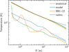 |
Fig. A.1 Comparison of 1D temperature profiles of the hydrostatic models at the end of the simulation for two different radiation methods — flux-limited diffusion (FLD, used in this work) and moment transfer (M1, Melon Fuksman & Klahr 2022). Overall we see very good agreement with temperatures with FLD and M1, with the optically thin atmosphere being captured quite well. The dotted black line shows the analytical solution for the temperature profile in the optically thin atmosphere (Chiang & Goldreich 1997). The midplane temperatures are also in good agreement, with some minor deviations. The M1 method shows higher amplitude bumps than the FLD method. We also include the RADMC-3D calculations corresponding to our FLD model, these correspond to the green lines. |
Appendix B H-band scattered-light synthetic observation
We post-processed the final temperature state from our fiducial radiation hydrodynamic model MFID using the radiation transfer code RADMC-3D (Dullemond et al. 2012) to produce synthetic scattered-light images that could be observed using VLT-SPHERE in the H Band (1.65 μm). We do not recompute the temperatures with radmc mctherm but we recalculated the dust opacities with optool (Dominik et al. 2021) with the same parameters as the ones used in this article (Krieger & Wolf 2020) to also include the scattering components. We then convolve the image using a Gaussian filter with a beam size of 40″ × 40″, and add a coronograph of the same size around the star. Figure B.1 shows the scattered-light image with the two starlight-driven bump and shadow pairs in our model having an imprint in the observables.
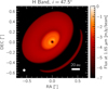 |
Fig. B.1 Synthetic scattered-light images in the H band of the final disk state in the fiducial model MFID. We chose a disk at a distance of 158 pc and an inclination of 47.5 deg similar to IM Lup (Avenhaus et al. 2018). The square in the bottom left denotes our beam size with a FWHM of 40″ × 40″. |
Appendix C Thermal relaxation timescale
Previous work has supported the idea that the ratio between the cooling timescale tcool and the dynamical timescale (≈![Mathematical equation: $\[\Omega_{\mathrm{K}}^{-1}\]$](/articles/aa/full_html/2026/02/aa56928-25/aa56928-25-eq27.png) ) is important in determining the formation and propagation of thermal waves (e.g., Dullemond 2000; Melon Fuksman & Klahr 2022). We therefore compute the cooling timescale to both assess its effect on the dynamics of the TWI as well as to estimate the radiative diffusion timescale between hydrostatic iterations in our models. For well-coupled dust and gas, the cooling parameter β = tcool ΩK can be written as a sum of optically thick and thin cooling components in the flux-limited diffusion approach (following Flock et al. 2017; Ziampras et al. 2024),
) is important in determining the formation and propagation of thermal waves (e.g., Dullemond 2000; Melon Fuksman & Klahr 2022). We therefore compute the cooling timescale to both assess its effect on the dynamics of the TWI as well as to estimate the radiative diffusion timescale between hydrostatic iterations in our models. For well-coupled dust and gas, the cooling parameter β = tcool ΩK can be written as a sum of optically thick and thin cooling components in the flux-limited diffusion approach (following Flock et al. 2017; Ziampras et al. 2024),
![Mathematical equation: $\[\beta=\frac{\Omega_{\mathrm{K}}}{\eta}\left(H^2+\frac{l^2}{3}\right), \quad \eta=\frac{16 \sigma_{\mathrm{SB}} T^3}{3 \kappa_P \rho^2 c_{\mathrm{V}}}, \quad l=\frac{1}{\kappa_P \rho}\]$](/articles/aa/full_html/2026/02/aa56928-25/aa56928-25-eq28.png) (C.1)
(C.1)
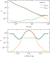 |
Fig. C.1 Top: Radial profile of the cooling timescale β for the disk. The regions of the disk where we find starlight-driven shadows lie in the intermediate cooling timescale regime (1–30 au). Bottom: Vertical profile of the cooling timescale β at R = 1 au. We see that for most of the disk (except for the atmosphere, and outermost regions), optically thick cooling is more dominant. |
where σSB is the Stefan-Boltzmann constant. We plot β radially and at a vertical slice corresponding to R = 1 au in Fig. C.1. Most of our radial computational domain is dominated by the optically thick component (∝ H2) until up to R ~ 50 au. We find starlight-driven staircases between 1–30 au, in regions corresponding to long-to-intermediate cooling timescales radially. Cooling is inefficient in the inner parts where the cooling parameter is as high as β = 103 and then it decreases reaching up to β = 0.1 at ~15 au. This indicates that the outer part of the disk is susceptible to the vertical shear instability (Nelson et al. 2013; Pfeil & Klahr 2019; Flock et al. 2020), as also supported by our study (see Fig.12). In the inner disk and along the vertical direction, the region around the midplane remains optically thick up to about four scale heights (|z|/r ≲ 0.12), with a rapidly cooling optically thin atmosphere where β ≲ 10−4. The spikes in the vertical profiles of the cooling timescale correspond to the numerical artifact in the temperature (see Fig. 6) and the flat profile in the upper disk boundaries corresponds to the density floor.
Appendix D The effect of τν,0 on the irradiation source term
In Sect. 6.6 we discussed the effect of the optical depth profile τν,0 at the inner radial end of our domain, given that it is an important initial condition that sets our disk model. We do not fully know the exact structure of the inner disk in reality. Starting out with shadows in the inner disk suggests that the disk outside of it could be subject to nonuniform heating. This could further help starlight-driven shadowing. In this section we compare the effect of two different profiles of τν,0 on the irradiation source term.
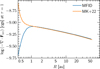 |
Fig. D.1 Comparison of the irradiation source term sampled at the τ = 1 surface for two different profiles for the initial optical depth τν,0. The blue line shows the profile used in this work while the orange line shows the profile used in Melon Fuksman & Klahr (2022). We see that they match very well outside 1 au but differ inward. While Melon Fuksman & Klahr (2022) use a radially decreasing, smooth profile, we see that our prescription can create little nonuniformities in heating that might affect the innermost bump. |
We compare the profile used in this work (Eq. (5)) with the one used in Melon Fuksman & Klahr (2022). Figure D.1 shows the irradiation source term sampled at the τ = 1 surface for both cases. We find very good agreement between the two prescriptions through most of the disk outward of 1 au. In the innermost parts, we note that the orange line (used by Melon Fuksman & Klahr 2022) is a smooth, radially decreasing quantity, while there is a little hotspot in the profile we use. This could influence the growth of the innermost bump in our model. Better models that motivate the inner disk structure from self-consistent radiation hydrodynamic models will help constrain this initial condition better. We nevertheless stress that the presence of a second bump (e.g., at 10 au in Fig. 6) is unaffected by this.
All Tables
All Figures
|
Fig. 1 Schematic to illustrate the different terms bump, shadow, and staircase defined in the introduction. The star is denoted by the orange blob, and the stellar rays hit the irradiation absorption surface τ⋆ = 1 at a height zs = z (τ⋆ = 1) from the midplane and a flaring angle φ. |
| In the text | |
|
Fig. 2 Top panel: frequency-dependent dust absorption opacities (per gram of dust, gdust) from tabulated values (Krieger & Wolf 2020, 2022). The blue points denote 132 frequencies logarithmically sampled in the range ν ∈ [1.5 × 10¹¹, 6 × 10¹⁵] Hz for the computation of irradiation flux in our models. The black line indicates the blackbody function, and the orange line shows the Planck opacity for T⋆ = 4000 K (figure similar to Kuiper et al. 2010). Bottom panel: temperature-dependent Planck and Rosseland mean opacities for the radiation transfer. The local maximum (≈ 250 K) and the subsequent dip in the mean opacities is due to the 10 μm silicate feature. |
| In the text | |
|
Fig. 3 Top: time evolution of the temperature profile at the disk midplane for iterations i = [10, 15, 20, 25, 30]. The profiles indicate that thermal waves form and travel inward with time. There are two bump and shadow pairs at the end of the hydrostatic run for model MFID. The dotted blue line is the radiation temperature at i = 30 and the dashed black line indicates the background power law fit for the midplane Tlaw = 185 (R/au)−0.5. Bottom: deviation of the temperature profile from the background power law. |
| In the text | |
|
Fig. 4 2D profiles of temperature and the irradiation heating term for the hydrostatic model at i = 30 iterations. The orange line refers to the τ⋆ = 1 profile for the stellar radiation using the Planck mean opacity. Blue lines refer to τν = 1 profiles for for different frequencies ν (same as in Fig. 2), with the line opacity weighted by Bν at that frequency. (see also Fig. 7 in Melon Fuksman & Klahr 2022). The red line indicates the τdisk = 1 profile for the disk’s radiation using κP(T). The green lines indicate the midplane gas scale height of the disk. |
| In the text | |
|
Fig. 5 2D profiles of temperature and the irradiation heating term for the hydrodynamic model at t = 500 orbits (top) and t = 10 000 orbits (bottom). The solid black line denotes the temperature corresponding to the opacity transition in Fig. 2. |
| In the text | |
|
Fig. 6 Top: time evolution of the temperature profile at the disk midplane against the background power law. The dashed lines (the first corresponds to the opacity transition) indicate the final locations of the temperature bumps. Bottom: time evolution of the radial temperature gradient indicating a less steep profile at the shadow locations and no sign flip. |
| In the text | |
|
Fig. 7 2D profiles of temperature and the irradiation source term for the MD0.001 hydrostatic+dynamic model with ϵdg = 0.001. Top panel: hydrostatic model after t = 30 iterations does not show any staircase structure. Bottom panel: hydrodynamic model after t = 500 orbits shows the innermost bump. |
| In the text | |
|
Fig. 8 2D profiles of temperature and the irradiation source term for the high surface density MSIG2000 hydrostatic+dynamic model. The hydrostatic run shows three prominent bumps (top), hydrodynamic run shows two bumps (bottom). Midplane temperature reached equilibrium after several radiative diffusion timescales, and hence the longer run time of t ≈ 12 000 orbits. |
| In the text | |
|
Fig. 9 Top: long-term time evolution of the midplane temperature deviation from the background power law for the dynamical model MSIG2000. After about t = 700 orbits, we see that the first and the second bump merge together. We can also spot an additional bump at ≈20 au. The dashed green line corresponds to the final state of the MFID model in Fig. 6, for comparison. Bottom: the evolution of the radial temperature gradient in time similar to Fig. 6. Here, we see that the innermost bump is a local maximum, producing a temperature gradient inversion, while the other two shadows produce slope changes in the profile. |
| In the text | |
|
Fig. 10 2D profiles of temperature and the irradiation heating term for the hydrostatic model with a dust tracer at i = 30 iterations for diffusion coefficients αD ∈ [0.0001, 0.001, 0.01]. We see a very sharp irradiation surface but there are no staircases formed in any of these models. |
| In the text | |
|
Fig. 11 Top: radial profile of the luminosity factor φ at the irradiation absorption surface showing a decreased incidence of stellar rays in the shadowed regions. Middle: radial profiles of the surface aspect ratio h at the τ⋆ = 1 surface. We see that the profiles deviate from a smooth power-law. Bottom: midplane radial pressure gradient shows deviations in the pressure profile. We note the flaring angle φ and the midplane pressure gradient d log Pmid/d log R are smoothed with a rolling average over 20 cells to eliminate noise. |
| In the text | |
|
Fig. 12 Vertical velocity profiles of the disk at t = 10 000 orbits normalized to the sound speed. We see the development of the VSI modes in the outer disk. The dashed line indicates the location where VSI is expected according to the Lin & Youdin (2015) criterion. |
| In the text | |
|
Fig. A.1 Comparison of 1D temperature profiles of the hydrostatic models at the end of the simulation for two different radiation methods — flux-limited diffusion (FLD, used in this work) and moment transfer (M1, Melon Fuksman & Klahr 2022). Overall we see very good agreement with temperatures with FLD and M1, with the optically thin atmosphere being captured quite well. The dotted black line shows the analytical solution for the temperature profile in the optically thin atmosphere (Chiang & Goldreich 1997). The midplane temperatures are also in good agreement, with some minor deviations. The M1 method shows higher amplitude bumps than the FLD method. We also include the RADMC-3D calculations corresponding to our FLD model, these correspond to the green lines. |
| In the text | |
|
Fig. B.1 Synthetic scattered-light images in the H band of the final disk state in the fiducial model MFID. We chose a disk at a distance of 158 pc and an inclination of 47.5 deg similar to IM Lup (Avenhaus et al. 2018). The square in the bottom left denotes our beam size with a FWHM of 40″ × 40″. |
| In the text | |
|
Fig. C.1 Top: Radial profile of the cooling timescale β for the disk. The regions of the disk where we find starlight-driven shadows lie in the intermediate cooling timescale regime (1–30 au). Bottom: Vertical profile of the cooling timescale β at R = 1 au. We see that for most of the disk (except for the atmosphere, and outermost regions), optically thick cooling is more dominant. |
| In the text | |
|
Fig. D.1 Comparison of the irradiation source term sampled at the τ = 1 surface for two different profiles for the initial optical depth τν,0. The blue line shows the profile used in this work while the orange line shows the profile used in Melon Fuksman & Klahr (2022). We see that they match very well outside 1 au but differ inward. While Melon Fuksman & Klahr (2022) use a radially decreasing, smooth profile, we see that our prescription can create little nonuniformities in heating that might affect the innermost bump. |
| In the text | |
Current usage metrics show cumulative count of Article Views (full-text article views including HTML views, PDF and ePub downloads, according to the available data) and Abstracts Views on Vision4Press platform.
Data correspond to usage on the plateform after 2015. The current usage metrics is available 48-96 hours after online publication and is updated daily on week days.
Initial download of the metrics may take a while.