| Issue |
A&A
Volume 706, February 2026
|
|
|---|---|---|
| Article Number | A191 | |
| Number of page(s) | 13 | |
| Section | The Sun and the Heliosphere | |
| DOI | https://doi.org/10.1051/0004-6361/202557427 | |
| Published online | 09 February 2026 | |
Solar limb faculae: Intensity contrast from two vantage points
1
Max-Planck-Institut für Sonnensystemforschung Justus-von-Liebig-Weg 3 37077 Göttingen, Germany
2
Instituto de Astrofísica de Andalucía (IAA-CSIC) Apartado de Correos 3004 E-18080 Granada, Spain
3
Institut d’Astrophysique Spatiale, Bâtiment 121, Rue Jean Dominique Cassini, Université Paris Saclay 91405 Orsay, France
★ Corresponding author: This email address is being protected from spambots. You need JavaScript enabled to view it.
Received:
26
September
2025
Accepted:
6
November
2025
Abstract
Context. Small-scale magnetic-flux concentrations contribute significantly to the brightness variations of the Sun, yet observing them – particularly their magnetic field – near the solar limb remains challenging. The Solar Orbiter mission offers an unprecedented second vantage point for observing the Sun. When combined with observations from the perspective of Earth, this enables simultaneous dual-viewpoint measurements of these magnetic structures, thereby helping to mitigate observational limitations.
Aims. Using such a dual-viewpoint geometry, we characterised the brightness contrast of faculae near the limb as a function of both their associated magnetic field strength and the observation angle.
Methods. We analysed data from the Polarimetric and Helioseismic Imager on board the Solar Orbiter (SO/PHI), obtained during an observation programme conducted in near-quadrature configuration with Earth, in combination with data from the Helioseismic and Magnetic Imager on the Solar Dynamics Observatory (SDO/HMI). The High Resolution Telescope of SO/PHI observed a facular region located near the disc centre as seen from its vantage point, while the same region was simultaneously observed near the solar limb by SDO/HMI. We identified faculae and determine their magnetic field strength from the disc-centre observations, and combined these with continuum intensity measurements at the limb to derive dual-viewpoint contrast curves. We then compared these with contrast curves derived from SDO/HMI alone.
Results. Using two viewpoints, we consistently find higher facular contrast near the limb than from a single viewpoint. A comparison of the facular line-of-sight magnetic field derived from limb observations with that derived from disc-centre observations (and re-projected to the limb) reveals significant differences between the two. Co-temporal observations of limb faculae from a second, disc-centre viewpoint enable a more precise determination of their associated magnetic field.
Key words: Sun: faculae / plages / Sun: magnetic fields / Sun: photosphere
© The Authors 2025
 Open Access article, published by EDP Sciences, under the terms of the Creative Commons Attribution License (https://creativecommons.org/licenses/by/4.0), which permits unrestricted use, distribution, and reproduction in any medium, provided the original work is properly cited.
This article is published in open access under the Subscribe to Open model.
Open Access funding provided by Max Planck Society.
1. Introduction
In the solar photosphere, active regions appear in the form of sunspots, pores, and faculae1. While large magnetic-flux concentrations, such as sunspots and pores, are seen as dark features, smaller concentrations manifest as faculae, which are typically brighter than the surrounding quiet Sun and are commonly interpreted in terms of magnetic flux tubes.
The intensity of faculae relative to the local quiet Sun (hereafter referred to as the intensity contrast) increases with the viewing angle from the disc centre towards the solar limb (e.g. Ortiz et al. 2002; Hirzberger & Wiehr 2005). This behaviour is best explained by the variations in optical depth of our observations with the angle at which we observe, which cause different portions of the flux-tube walls to become visible. The walls of flux tubes appear bright due to the “hot-wall effect” (see, Spruit 1976), leading to the observed intensity variation (see simulations from, e.g. Carlsson et al. 2004; Steiner 2005). The change of the intensity close to the extreme limb is less certain, and studies historically disagree on whether the intensity increases continuously or if it decreases at the extreme limb (see Solanki 1993 for an overview).
More recent studies, based on full-disc observations, such as Yeo et al. (2013) and Ortiz et al. (2002) find a decrease when approaching the limb, which is attributed to the surrounding granulation eventually obscuring these small structures. The intensity contrast of faculae at different viewing angles also depends on their associated magnetic field strength. Faculae with stronger magnetic fields generally appear brighter near the limb and darker near the disc centre than those with weaker fields. This is attributed to the correlation of the magnetic field strength to the size of the faculae. The relationship between facular intensity contrast and magnetic field strength has been examined in studies such as Kobel et al. 2011; Kahil et al. 2019 (see also references therein), while characterising this relationship as a function of the observation angle has been addressed in works such as Ortiz et al. 2002; Yeo et al. 2013; Albert et al. 2023; this is also the goal of the present study. Beyond insight into the physics of flux tubes, these studies provide essential information for solar irradiance models spanning timescales ranging from days to millennia (see Krivova et al. 2003; Solanki et al. 2013; Yeo et al. 2017; Wu et al. 2018; Chatzistergos et al. 2025).
Observing faculae, however, remains challenging, primarily because the underlying magnetic elements are frequently small (∼150 km). In most cases, and in particular in full-disc observations, they are not spatially resolved, even at the disc centre. Consequently, the analysis of facular observations must account for the spatial averaging of signal from the flux tubes (with strong magnetic fields and high intensity contrast) and their surroundings (with considerably lower magnetic fields and intensity contrast) within each resolution element. This challenge becomes even more severe near the solar limb. As the viewing angle increases, each resolution element covers a larger surface area due to projection effects, further reducing the effective spatial resolution.
In addition, radiative transfer effects complicate the interpretation of observations away from the disc centre. Compared to disc-centre observations, at the limb, the same optical depth corresponds to higher atmospheric layers, which are generally cooler, leading to various effects. Firstly, this causes limb darkening, which decreases the signal-to-noise ratio (S/N) of limb measurements across all Stokes parameters. Radiative transfer effects that influence brightness and contrast are part of the investigated phenomenon (how the intensity of faculae changes with the observation angle). However, the same effects also impact the measured Stokes profiles, and, therefore, the inferred magnetic quantities. This is undesirable: the magnetic field would ideally be retrieved consistently across the disc, without differences in optical depth and line-of-sight geometry, allowing us to establish the variation of the intensity in relation to observation angle and the magnetic field strength coherently. The amplitude of the Stokes V profile does not necessarily scale linearly with μ, as a consequence of radiative transfer effects. Most notably, at high viewing angles, due to the narrow nature of these structures, light may pass through both magnetic and non-magnetic regions. This leads to the Stokes profiles accumulating signal from various regions (see Solanki et al. 1998; Sinjan et al. 2024).
In studies of solar faculae, the line-of-sight component of the magnetic field (BLOS) is typically used as a measure of magnetic field strength due to its greater reliability compared to the full vector magnetic field. However, deriving the magnetic field strength from the BLOS is not straightforward. In the absence of information on the magnetic field orientation, the BLOS is commonly divided by the cosine of the heliocentric angle (μ = cos θ), based on the assumption that facular magnetic fields are oriented radially with respect to the solar surface. Under this assumption, the division acts as a geometrical correction, yielding a representative magnetic field value. However, facular magnetic fields are only radial on average; therefore, this assumed geometrical correction – i.e. dividing the BLOS by μ – introduces errors. Assuming a roughly symmetric, fanning-out configuration of field lines in facular structures, the geometrical re-projection of the field lines to the limb introduces systematic, strongly asymmetric biases in the line-of-sight component. If the same structure were observed at disc centre, the derived BLOS would underestimate the magnetic field strength, but no asymmetry would be introduced. See, for example Leka et al. (2017) for further discussion on using the BLOS to approximate the vector magnetic field, Centeno et al. (2023) for related effects, and Calchetti et al., in prep., for effects observed in polar faculae.
Moreover, the BLOS presents further disadvantages at the limb. Most importantly, for nearly surface-radial magnetic fields, the line-of-sight component diminishes towards the limb, leading to lower signal levels. These levels are often comparable to the noise level of the observations (which is also increased at the limb, even in ideal conditions, by photon noise), even for relatively strong fields, such as those associated with faculae. Moreover, limb observations probe higher atmospheric layers, where magnetic structures are more expanded and appear larger and more horizontal. The signal from these magnetic canopies can significantly contribute to the Stokes V signal, altering the observed magnetic landscape (see Giovanelli & Jones 1982; Solanki et al. 1994; Pietarila et al. 2010; Ball et al. 2012; Yeo et al. 2013; Albert et al. 2023). Both of these effects hinder the reliable identification of faculae near the limb based on the BLOS.
Due to these observational limitations, the relationship between the contrast of faculae and the magnetic field strength near the limb remains uncertain in single-viewpoint studies (as in, e.g. Ortiz et al. 2002; Yeo et al. 2013). A second viewpoint, where regions near the limb appear closer to disc centre, can help overcome some of these challenges. This approach was demonstrated by Albert et al. (2023), combining data from the Full Disc Telescope of the Polarimetric and Helioseismic Imager on board the Solar Orbiter (SO/PHI-FDT, Müller et al. 2020; Solanki et al. 2020) and the Heliosismic and Magnetic Imager on board the Solar Dynamics Observatory (SDO/HMI, Pesnell et al. 2012; Schou et al. 2012). They analysed co-observations taken at line-of-sight angles separated by 60° and demonstrated that facular contrast can be determined much closer to the limb in the dual-viewpoint than in single-viewpoint analyses. This first study employed SO/PHI-FDT data which was acquired at a large distance from the Sun, and therefore had low resolution.
In the current work, we used high-resolution observations. We analysed co-temporal observations of a facula-rich region obtained by the High Resolution Telescope of SO/PHI (HRT; Gandorfer et al. 2018) and by SDO/HMI in a near-quadrature configuration, where the region appears close to disc centre from the perspective of SO/PHI-HRT and near the limb from the viewpoint of SDO/HMI.
2. Methods
The data used in this study were acquired as the Solar Orbiter emerged from behind the Sun from Earth’s viewpoint, crossed quadrature, and approached the Sun-Earth line. During this period, the same region appeared at varying disc positions in SDO/HMI data, spanning from the extreme limb to a μ of around 0.7. Figure 1 shows the observing geometry of the two spacecraft. These data provide an unprecedented opportunity to complement our understanding of facular magnetic fields at the limb through simultaneous observations of the same region from the disc-centre viewpoint.
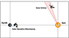 |
Fig. 1. Sketch of observing geometry between Solar Dynamics Observatory (SDO) and Solar Orbiter for observations used in the study. The coordinate system is with the Earth and the Sun at fixed positions, as seen from above. While SDO observes the Sun from the Earth’s perspective, on the horizontal black line, the Solar Orbiter varies its view angle between the two red lines, moving from right to left (i.e. approaching the Sun-Earth line). The spacecraft illustrations are provided courtesy of ESA and NASA. |
Deriving the facular contrast as a function of magnetic field strength and observation angle (we call the resulting curves, intensity contrast curves), includes three key components: (1) the intensity contrast; (2) the magnetic field strength; and (3) the identification of faculae, which we based on the magnetic field. Our aim is to improve on some of the observational constraints at the limb by incorporating a BLOS obtained from a disc-centre-viewpoint into our analysis. In our study, we used (1) the contrast derived from SDO/HMI observations at the limb; (2) the BLOS derived at the disc centre in SO/PHI-HRT and re-projected to the limb, resulting in spatial averaging of the SO/PHI-HRT pixels; and (3) the facular map derived at the disc centre from SO/PHI-HRT, and re-projected to the limb (with the method used for the BLOS).
The combination of intensity contrast observed at the limb with BLOS and facular map derived at the disc centre is only possible under the assumption that the continuum contrast only changes in magnitude when going from disc centre to the limb, but the physical area in which the contrast enhancement is observed does not become larger or smaller (other than the geometrical effect of a different view-angle). Steiner (2005) found that the apparent size of faculae (i.e. the spatial extent of contrast enhancement) changes at most by 87 km at various view angles (measured in the plane of the sky). This is below the pixel size of SO/PHI-HRT even at the disc centre at perihelion (≲130 km), and therefore the effect is negligible in our observations.
2.1. The observations
We used data from a SO/PHI-HRT observational campaign in October 2022, conducted under the RSMALLMRESMCADAR-Long-Term Solar Orbiter Observing Plan (SOOP, Zouganelis et al. 2020). At that time, from Earth’s perspective, Solar Orbiter was approaching the Sun-Earth line. Observations were carried out near the disc centre in the SO/PHI viewpoint (at μ > 0.8), at heliocentric distances ranging from 0.35 to 0.37 au. Given the 0.5″ plate scale of the HRT, this corresponds to 127 km – 134 km on the Sun per pixel at the disc centre, and one observation is conducted in 85 s. The Solar Orbiter tracked a region containing two largely unipolar groups of faculae, with several small pores located at the larger magnetic concentrations in both polarities.
We analysed 34 SO/PHI-HRT magnetograms from this campaign, recorded between 2022.10.20 21:15:03 and 2022.10.22 21:15:03 UTC. Specifically, we used the soloL2phi-hrt-blos data product, which is processed entirely on the ground (see Sinjan et al. 2022; Kahil et al. 2023; Bailén et al. 2024). The BLOS values are derived from the vector magnetic field, inferred using the cmilos RTE inversion code (see Orozco Suárez & Del Toro Iniesta 2007).
The SDO/HMI instrument operates on the same principle as SO/PHI. To ensure the best temporal alignment and consistency between the two instruments, we used SDO/HMI 45 s data products. For the BLOS, we used hmi.M45s, computed with the so-called MDI-like algorithm (named after the Michelson Doppler Imager instrument on the Solar and Heliospheric Observatory, using a similar technique; see Scherrer et al. 1995). This method computes Dopplergrams in the right and left circularly polarised light and derives the magnetic field from their difference. For continuum intensity, we used the hmi.Ic45s data product, which estimates the Ic from the Doppler shift, line width, and line depth, assuming a Gaussian line profile (see Couvidat et al. 2016).
We selected the SDO/HMI observations closest in time to each SO/PHI-HRT magnetogram. We did not apply any cross-calibration of the magnetic field between the instruments, as Sinjan et al. (2023) showed that the chosen data products agree well. Figure 2 shows the first and last dataset pairs in the data series used in this study. At the time of the observations, Solar Orbiter partially co-rotated with the Sun. As a result, the region remained near the disc centre in the SO/PHI-HRT view, while in the SDO/HMI view it moved from close to the limb towards the disc centre. Thus, the first dataset corresponds to the largest angular separation, with the region closest to the limb in HMI, while the last shows the same region closer to disc centre.
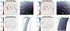 |
Fig. 2. First and last dataset pairs used in this study, from 20 and 22 October 2022 (A and B, respectively). Top: BLOS and μ of a facular region near disc centre (a and b). Bottom: BLOS and μ of same region, as seen simultaneously by SDO/HMI (c and d). The contour shows the location of the SO/PHI field of view, and the μ in the SDO/HMI view-point is shown only for the contoured region. |
Figure 3 highlights the significant increase in detail in BLOS provided by the SO/PHI-HRT owing to its higher spatial resolution and its disc-centre view-point compared to the limb view from SDO/HMI in the first dataset used in our study. We exploited the high resolution of the HRT data in two ways: it allowed us to reliably identify faculae, and it ensured that, after degrading the magnetic field maps to the limb resolution for pixel-to-pixel comparison, the resulting data retained much lower noise levels.
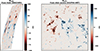 |
Fig. 3. Co-observation of BLOS in same region at the limb (SDO/HMI, left) and at disc centre (SO/PHI-HRT, right), from the first dataset pair in our study. The SO/PHI observation time was 2022-10-20T21:15:46, which corresponds to 2022-10-20T21:20:28 at Earth after accounting for light travel time (in UTC). The SDO/HMI observation time was 2022-10-20T21:19:58 UTC. |
2.2. Changing geometric perspective from disc centre to limb
We analysed pairs of datasets that capture the same region from two different viewing angles: with SO/PHI-HRT near disc centre and SDO/HMI near the limb. To enable such an analysis, we must associate each limb-pixel with a corresponding value, originating from the disc-centre observations. Besides geometrical mapping (i.e. bringing them to a common reference frame), we must also account for foreshortening – that is, the same pixel covers an increasingly larger area on the solar surface as the observation angle increases. Additionally, the spatial resolution of the two instruments is also different.
We changed the perspective of the disc centre observation (by SO/PHI-HRT) to that of the area observed at the limb (by SDO/HMI), using the re-projection algorithm described in (DeForest 2004), as implemented in SunPy Community et al. (2020). This method associates each limb pixel with its footprint (i.e. contributing pixels) at the disc centre and assigns the mean of the footprint pixels as the value of the pixel. We used the Hann window option of the algorithm for weighting the mean, which we found to provide the best balance between magnetic-flux conservation and re-sampling to the lower resolution of the limb observations, specifically avoiding additional smoothing of the results. This process simultaneously accounts for the foreshortening effect caused by observing the same area from different viewing angles and the difference in spatial resolution between the two instruments, and we did not apply prior spatial degradation to the SO/PHI data. We used the term re-projection, following (DeForest 2004), but we note that there is no vector re-projection performed, just a re-mapping or re-sampling of the pixels.
For the reference frame used in the geometrical mapping, we rely on the georeferencing of the datasets (expressed in the World Coordinate System framework, WCS, see Thompson 2006). For full-disc observations, such as those from SDO/HMI, we can take the disc centre as a reference, which can be determined with high accuracy by using limb-fitting algorithms. In contrast, the SO/PHI-HRT data used in the study lack clear reference features such as the solar limb within its limited field of view. Consequently, its WCS coordinates rely on the spacecraft’s attitude determination, which is less precise. To improve the accuracy of the SO/PHI-HRT WCS coordinates, we first re-projected the SDO/HMI data to the SO/PHI reference frame and performed a cross-correlation between the two. The resulting shift was then used to update the WCS entries to the SO/PHI-HRT data.
After updating the WCS coordinates of the SO/PHI-HRT data, we applied image-distortion corrections and re-projected the data into the SDO/HMI reference frame. To identify residual misalignment, we computed the cross-correlation between the re-projected SO/PHI BLOS and the Ic provided by SDO/HMI near the limb. We refined the alignment to sub-pixel accuracy by fitting a quadratic surface to the 3 × 3 pixel region surrounding the correlation peak and calculating its maximum. This ad hoc alignment assumes that the disc-centre and limb views correspond to the same solar region without any significant parallax effect.
2.3. Viewing-angle compensation of BLOS
Due to the evacuated nature of magnetic flux tubes, faculae are buoyant in the surrounding granulation, and, on average, they exhibit surface-vertical orientation (see, e.g. Knoelker & Schüssler 1988; Schüssler 1992). Therefore, the line-of-sight component of the magnetic field, BLOS, decreases towards the limb. This is commonly compensated by dividing BLOS by μ, which is a simple geometrical correction under this surface-radial assumption (see also Murray 1992).
Facular structures are not strictly radial, however. They expand with height (Solanki et al. 1999). In observations of faculae near the limb, a reversal in magnetic polarity is observed for the limb-ward sides of facular regions (see Pietarila et al. 2010). This is due to the fact that the inclined fields at observation angles larger than their inclination tilt away from the observer, and they show a reversal of their polarity in the BLOS. These observations indicate that the structures in facular regions are sufficiently inclined to introduce strong asymmetric biases in the derived BLOS at large heliocentric angles. Meanwhile, we can expect that approximating the magnetic field strength with BLOS/μ at or close to the disc centre underestimates the magnetic field due to the inclined field lines, but it does not introduce strong asymmetries. By incorporating simultaneous disc-centre observations from a second viewpoint, we can determine the magnetic field strength of facular structures near the limb without the strong biases affecting limb measurements, and we can ensure consistency across all viewing angles.
2.4. Continuum intensity contrast
The continuum intensity contrast quantifies the brightness of facular features relative to their local surroundings. In this study, we used the contrast derived exclusively from the SDO/HMI viewpoint.
To begin, we calculated the normalised intensity, Ic, norm.(x, y, t), by dividing the continuum intensity images by the local μ-dependent mean quiet-Sun intensity, where x and y are the spatial dimensions and t denotes time. This relationship is similar to the commonly used centre-to-limb variation (CLV) of solar intensity, with the distinction that it accounts not only for limb darkening but also for stray light and other instrumental artefacts. We determine this relationship in the individual datasets by computing the mean intensity of the quiet-Sun regions (defined as regions where |BLOS|< 2 * σ, σ being the noise level of SDO/HMI) as a function of μ. We sorted the Ic data by μ and grouped them into bins of 5000 pixels. The mean intensity in each bin was then fitted with a 20th-order polynomial, which provides an accurate representation of the intensity variation for μ > 0.035 (see Appendix B for further details).
The continuum intensity contrast, CIc(x, y, t), was then calculated as
 (1)
(1)
2.5. Identification of faculae
We identified faculae based on their associated BLOS values following the approach of Albert et al. (2023) applied in the respective observed coordinate systems. The result of this identification is referred to hereafter as the ‘facular map’. A pixel is classified as facular if it is part of a contiguous structure, exceeds three times the noise level in BLOS, and is not dark (i.e. not a sunspot or pore, assessed based on an intensity threshold). We confirmed the robustness of the three-times-noise-level threshold by increasing it to four, which yielded no significant change in the results.
For SDO/HMI, the noise level follows a centre-to-limb variation, which we determined using the method described in Albert et al. (2023). However, in contrast to Albert et al. (2023), we did not account for field-of-view-dependent residual variations in the noise additional to the centre-to-limb changes. We note that the noise levels at the east and west limbs may deviate by up to 1 G from the mean noise level due to the radial velocity of SDO (private communications, A. Kumar Yadav); however, we do not account for these variations. The derived noise level ranges from 10.2 G near the limb to 8.6 G at the disc centre. These values are largely consistent with those reported by Liu et al. (2012) at the disc centre, although they are somewhat lower at the limb.
In addition to the BLOS threshold, we applied an intensity-based criterion to exclude sunspots and pores in the full-disc SDO/HMI data, following Albert et al. (2023). Specifically, any pixel with a continuum intensity below a certain threshold was excluded. This threshold is defined as the mean of the minimum values of Ic, norm.(x, y, t)−3σIc, QS(x, y, t) across all observations, where σIc, QS is the standard deviation of the quiet-Sun continuum intensity (i.e. of those pixels that did not classify as faculae). We note that this facular map is only used for the reference results from a single-viewpoint, for which we used SDO/HMI data from the full disc (see Fig. 6).
For SO/PHI, we assumed a uniform BLOS noise level of 10 G across the entire field of view. Since the observed region at the disc centre contains no sunspots or large pores – except for small pores, which appear bright near the limb, and hence also contribute to the facular brightness there – we did not apply additional intensity-based selection criteria.
The facular map determined from SO/PHI was re-projected to the SDO/HMI coordinate system. Since we mapped data from the disc centre to the limb, the projected area becomes compressed, meaning that multiple disc-centre pixels – with potentially not all of them being classified as the same type of structure – contribute to a single pixel at the limb. As a result, the re-projected facular map contains pixels with varying degrees of facular contribution. To ensure that only pixels with sufficient facular contribution are included in our analysis, we applied an additional filtering criterion: any pixel for which the re-projected BLOS/μ from SO/PHI-HRT falls below the SDO/HMI BLOS noise level at the limb was excluded (see also Albert et al. 2023). The excluded pixels typically lie at the peripheries of facular regions or correspond to small, scattered flux concentrations, consistently with the effects of reduced spatial resolution (see Fig. A.1 in Appendix A).
3. Results
3.1. Comparison of the two viewpoints
We begin by comparing the BLOS and BLOS/μ values derived at the limb from SDO/HMI with the BLOS/μ of the same region, derived from disc-centre co-observations by SO/PHI and re-projected to the limb. In Fig. 4, we show a sub-region of the first dataset pair used in our analysis, where the observed area lies closest to the limb in SDO/HMI (μ < 0.4).
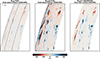 |
Fig. 4. Sub-region of first dataset pair in time series used in the study, showing BLOS derived from the limb observation by SDO/HMI (first panel), the same data divided by μ (BLOS/μ, second panel), and BLOS derived from disc centre by SO/PHI-HRT; these are divided by the μ value of the disc-centre view and re-projected to the limb to match the reference frame of SDO/HMI (third panel). |
A key difference between the two viewpoints is that the same region shows patches of a largely unipolar BLOS at the disc centre, while it exhibits a polarity reversal at limb – which is similar to what is observed for sunspots. This behaviour is consistent with previous findings by Pietarila et al. (2010), and here we confirm these for the first time from an independent vantage point. The underlying cause is the expansion of the magnetic structures with height, which leads to the inclination of the magnetic field lines relative to the surface normal (as also modelled in Pietarila et al. 2010). On the disc-centre-facing side of a fanned-out structure, the field lines point towards the observer, maintaining the same polarity as observed at the disc centre. On the limb-facing side, however, the field lines tilt away from the observer, resulting in the reversal of their polarity in the observed BLOS (see also, Giovanelli & Jones 1982; Solanki et al. 1994). This also leads to the appearance of a polarity reversal line, with close-to-zero BLOS values in the magnetograms at the limb.
Including a simultaneous disc-centre viewpoint of the limb faculae offers two key advantages in the analysis. First, deriving the magnetic field of limb faculae from the disc-centre viewpoint reduces the biases present in limb observations (such as geometrical projection and foreshortening effects, which are detailed in Sect. 1). This ensures a more consistent determination of the facular magnetic field across the solar disc. Second, because in this study faculae are identified based on their associated magnetic field (see Sect. 2.5), a more accurate field determination leads to a more reliable facular map at the limb.
3.2. Intensity-contrast curves
Figure 5 illustrates the combination of data used in the double-viewpoint analysis, showing a sub-region of the first data pair included in the study. The data were processed as described in Sect. 2.
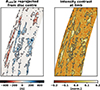 |
Fig. 5. Data combined in our analysis from different viewing angles. Left: BLOS derived at disc centre from SO/PHI-HRT observations, normalised by the local μ at which it was observed and reprojected to the limb. Right: Intensity contrast is computed from SDO/HMI Ic data at the limb. Contours: We identified facular pixels at disc centre in SO/PHI-HRT observations and then re-projected this map to the limb. The same sub-region as in Fig. 4 is shown. |
To characterise the CIc of faculae as a function of both the associated BLOS/μ and μ, we derived intensity contrast curves (CIc versus μ) for different BLOS/μ categories (Fig. 6). Faculae are grouped into eight categories based on their BLOS/μ values. Within each category, the data are binned in intervals of Δμ = 0.03. Only points with μ ≥ 0.05 were considered, and any bin with fewer than ten points was disregarded.
Figure 6 presents the centre-to-limb variation of the facular continuum contrast. This is shown separately for eight bins in BLOS/μ in the different panels. In each panel two curves are plotted: a reference derived from a single viewpoint (from SDO/HMI, shown in orange), and the results of our double-viewpoint approach (combining SDO/HMI and SO/PHI-HRT in their overlapping region, shown in green). The markers represent the mean CIc within each bin, while the shaded regions indicate the standard deviation.
The orange curves are derived from the full solar disc observed in SDO/HMI, and therefore show comparable results to those of Yeo et al. (2013). There are two major differences in how the SDO/HMI data were treated in Yeo et al. (2013) and in our study. Yeo et al. (2013) (1) averaged seven consecutive hmi.M45s data products and (2) used a total of 15 datasets, spanning a period longer than a year. In contrast, in this study we (1) used single hmi.M45s magnetograms and (2) based our statistics on 34 datasets, recorded over two days. The largest difference in the results is that the noise level was lower in the averaged magnetograms, leading to the curves extending closer to the limb in Yeo et al. 2013. Apart from this aspect, the results agree well.
The green curves, derived using the double-viewpoint approach, show that for faculae associated with lower magnetic field strengths (BLOS/μ < 180 G), the method enables intensity contrast observations significantly closer to the limb than the single-viewpoint approach (as also demonstrated by Albert et al. 2023). Additionally, we find a few faculae linked to strong magnetic fields (BLOS/μ > 640 G) near the limb in the double-viewpoint results; these are marked by the green curves that do not extend all the way to the limb in panels (a) to (c). This is a consequence of the magnetic field now being derived at the disc centre and therefore showing lower values (see also Sect. 3.1 and Appendix C). These contrast curves also exhibit trends distinct from those of the single-viewpoint curves. In the single-viewpoint case, the contrast generally increases smoothly from the disc centre toward the limb before gradually decreasing (as also observed by Ortiz et al. 2002; Yeo et al. 2013). In comparison, the double-viewpoint results show a close-to-linear increase in contrast toward the limb, followed by a sharp drop.
Figure 7 shows the pixel counts in each bin for both single- and double-viewpoint methods. In the single-viewpoint case, stronger magnetic fields are predominantly detected near the limb, producing an artificial distribution in which high-field faculae appear more frequently at low μ values than closer to the disc centre. This contradicts the expectation that BLOS measured at lower spatial resolution (larger pixels near the limb) should be reduced by averaging with neighbouring signal, rather than being enhanced relatively to the higher resolution disc-centre view. In contrast, the double-viewpoint method produces a more balanced distribution, with most pixels concentrated at intermediate μ values and gradually decreasing towards the extremes. This pattern aligns with the motion of Solar Orbiter during the observations, moving from quadrature towards the Sun-Earth line and corresponding to 0 ≤ μ ≤ 0.75 in SDO/HMI. Consequently, the overlapping area of most datasets – and thus the region with increased statistics – is centred around intermediate μ values of the observed range. With this new distribution, however, we have low statistics in the higher magnetic field categories, as well as in regions close to the limb.
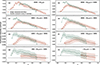 |
Fig. 6. Relationship between facular intensity contrast and μ. Panels (a)–(h) show pixels grouped by their associated BLOS/μ values. Points represent the mean intensity contrast in μ bins of width 0.03; shaded areas indicate the standard deviation within each bin. Orange dots correspond to a single-viewpoint analysis using SDO/HMI data from the full disc. Green triangles represent results from the dual-viewpoint approach, combining SO/PHI-HRT observations at the disc centre with SDO/HMI observations near the limb in the region of overlap. Note that the y-axis limits differ between panels. |
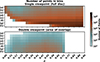 |
Fig. 7. Number of pixels averaged in each μ bin for the results in Fig. 6. The y-axis is labelled from ‘a’ to ‘h’ in accordance with the panel identifiers in Fig. 6. Top panel: Single-viewpoint case (orange dots in Fig. 6). Bottom panel: Double-viewpoint case (green triangles in Fig. 6). A logarithmic colour scale is used. Note that the single-viewpoint analysis has more pixels overall, as we consider the entire solar disc, as opposed to the small, overlapping field-of-view region in the double viewpoint. |
The observation angle at which facular contrast reaches its maximum (μmax) has long been debated (see Solanki 1993), and observations disagree due to differences in, for example, observational resolution and facular identification methods (see Centrone & Ermolli 2003; Auffret & Muller 1991). In our results, the maximum contrast lies systematically closer to the limb, especially in the lower magnetic field cases (panels d-h), than observed from a single viewpoint. However, especially in panels (a)–(c), the statistics are too low to form a clear peak. While in panels (d)–(h) we can identify a clear peak, this lies so close to the limb that the decrease after the peak is defined by only a few points, which all have relatively low statistics. Therefore, due to the limited statistics, we did not fit a curve to our results to determine the μmax (as in, e.g. Albert et al. 2023; Yeo et al. 2013).
4. Discussion
The observed differences between the single- and double-viewpoint contrast curves in Fig. 6 arise from two main factors: (1) the pixels in the analysis are selected based on the new facular map derived at disc centre, and (2) the magnetic field values associated with the faculae are likewise taken from disc-centre observations. Since faculae are identified via their associated BLOS values, both effects ultimately reflect the differences between the magnetic landscapes seen at the limb and at the disc centre (Fig. 4).
Figure 8 highlights the discrepancies between the facular maps derived from limb data (based on SDO/HMI) and disc-centre data (based on SO/PHI) re-projected to the limb. Using the disc-centre identification as a reference, only 44% of faculae are correctly identified in the data gathered near the limb, while 56% are missed – mainly along the edges of the facular regions. However, some of the smaller facular structures were entirely undetected. There are also a number of pixels identified as faculae at the limb, that do not qualify as faculae from the disc centre. These are mainly along the edges of the facular structures, with some smaller concentrations scattered around the region. The latter could be the signature of horizontal magnetic fields at the extreme limb (see, e.g. Lites et al. 2008; Danilovic et al. 2010). Figure 9 shows the intensity contrast of the pixels identified as faculae at the limb, and at the disc centre. The disc-centre identification outlines the contrast enhancement better, while the limb identification includes many dark pixels and misses bright pixels in the centre of the structure, also shown in the histogram.
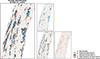 |
Fig. 8. Differences in faculae identification between direct limb observations (as in state-of-the-art studies) and identifications performed on disc-centre data, with the results re-projected to the limb (this study). Colour B shows facular pixels identified both at the disc centre and at the limb, while colour C shows the faculae missed at the limb compared to the disc-centre view. Colour D shows pixels identified as faculae in the limb data, which do not appear as faculae at the disc centre. The same sub-region and dataset pair as in Fig. 4 is shown. |
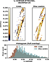 |
Fig. 9. Intensity contrast of a facular region at the limb. Left: Facular pixels are identified at the limb. Right: Facular pixels are identified at the disc centre. Bottom: Histogram of pixels in the top left and right panels. We show a sub-region of the first dataset in the study, corresponding to μ < 0.2. |
Using the magnetic field derived at the disc centre instead of the limb causes pixels to be reclassified among the different magnetic field categories. Figure 10 illustrates an example of how the BLOS/μ categories differ between centre and limb views. Pixels are coloured according to their assigned category. In the limb view, pixels falling into the higher magnetic field categories are found at the edges of the structures, while a line of pixels in the lowest categories runs through their centres, corresponding to the location where the polarity reverses at the limb. In contrast, the centre view offers a natural distribution, where the centre of the region falls into the strongest field categories, and the edges into the weaker ones. These differences in categorisation are consistent with Fig. 7, which shows that a single viewpoint leads to an over-population of the high magnetic field categories at the limb.
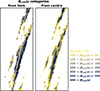 |
Fig. 10. Sub-region of the first dataset pair in the study, illustrating the change in BLOS category of facular pixels between vantage points. Left: Limb view. Right: Disc-centre view. The categories (a to h in Fig. C.1) are assigned colours ranging from blue to yellow, which are used to colour the pixels in the images. Same region as in Figure 9. |
The differences shown in Fig. 10 result from the expansion of magnetic structures with height, which causes field lines to deviate from the radial direction at the edges of facular regions. Although these fields appear weaker at disc centre, their inclination enhances the Stokes V signal near the limb, resulting in higher BLOS values than a purely radial field would. Dividing by μ then amplifies these values further, leading to the misinterpretation of such pixels as high magnetic field regions at the limb.
For more insight into the differences between the single- and double- viewpoints, an intermediate step between the two curves of Fig. 6 is presented and discussed in Appendix C.
5. Conclusions
The SO/PHI instrument, when combined with assets on Earth, or orbiting Earth, provides unprecedented opportunities to study photospheric magnetic structures from two viewpoints. A first demonstration of the advantages of a second viewpoint in the study of faculae was presented by Albert et al. 2023, who combined data from the SO/PHI-FDT and SDO/HMI at a 60° line-of-sight separation. That study showed not only that a second viewpoint enables the observation of facular contrast closer to the limb, but also that systematic differences arise between single- and double-viewpoint results near the limb, mainly because magnetic field measurements are less reliable close to the limb.
We extended the analysis of Albert et al. 2023 to high-resolution SO/PHI-HRT observations taken as the Solar Orbiter emerged from behind the Sun from Earth’s viewpoint, approaching the Sun-Earth line and approximately co-rotating with the Sun. SO/PHI-HRT followed a facular region observed roughly at disc centre from the SO/PHI perspective. The same region, as the Sun rotated into view, appeared at different angles in SDO/HMI, ranging from the limb to μ ∼ 0.8. Our study consists of two main components: (1) a direct comparison of the facular observations near the limb (as seen by SDO/HMI) and at disc centre (as observed by SO/PHI-HRT), and (2) an analysis of the facular contrast as a function of the associated BLOS and μ obtained by combining the two viewpoints. The results thus obtained are compared with those from just a single viewpoint.
Comparing the BLOS/μ of the region measured at the limb by SDO/HMI with that measured at the disc centre by SO/PHI-HRT and re-projected to the limb, we find that facular regions at the limb exhibit a polarity reversal in their line-of-sight magnetic fields, consistent with the findings of Pietarila et al. 2010. Here, we verified this behaviour for the first time from a second viewpoint. This is best explained by the expansion of the magnetic field of individual unresolved faculae with height. Groups of such faculae form a ‘facular bouquet’ configuration (Pietarila et al. 2010). In this configuration, flux tubes at the periphery of facular areas (adjacent to quiet-Sun regions) are more inclined than those at the centre of the facular complex. This large-scale organisation is discernible in the observations and gives rise to the observed polarity reversal, when viewed at large angles. As a result of the expansion with height, most of the magnetic field lines in facular regions are not normally directed to the local solar surface, even if that is the case on average. Consequently, the line-of-sight component of the magnetic field carries insufficient information to describe the strength of the magnetic field in faculae (see also Leka et al. 2017, for a more detailed discussion). In principle, a similar analysis could be performed using the strength of the vector magnetic field (|B|) to mitigate biases at the limb; however, the higher noise levels in |B| considerably limit the applicability of this approach.
As a consequence of the differences in the derived magnetic field, facular identification methods based on BLOS produce substantially different facular maps from disc-centre and limb perspectives. In the first observation of our time series (corresponding to the largest viewpoint separation), we find that less than half (44%) of the faculae identified at disc centre are successfully detected at the limb. Many faculae associated with weaker magnetic fields are missed (56% of disc-centre facular pixels), while false positives also occur, accounting for 27% of the disc-centre facular map when re-projected to the limb. These false positives falsely associate a significant amount of non-facular signal with magnetic features in single-viewpoint near-limb intensity-contrast studies.
Comparing the facular intensity-contrast curves derived from the double-viewpoint approach (using SO/PHI-HRT and SDO/HMI) to those obtained from a single viewpoint (using SDO/HMI only), we find that the facular intensity contrast towards the limb is systematically higher in the double-viewpoint case, particularly for faculae associated with weaker magnetic fields. Additionally, we observe that the angle at which the maximum contrast (μmax) occurs in the double-viewpoint approach is located closer to the limb. However, the statistics of the current study are too limited to reliably determine the value of μmax. These findings differ from the results of Albert et al. 2023, likely due to several factors: (1) the lower resolution of the SO/PHI-FDT dataset used in that study; (2) the fact that the reference ‘disc-centre’ observations in that study spanned a wide μ range (0.4 < μ < 1), thereby still incorporating limb effects; and (3) the derivation of μmax being based on a combination of single- and double-viewpoint observations (above and below μ = 0.4, respectively). The main limitation of the present study, however, remains the restricted statistics. Since we observed only a single region over several days, the dataset lacks a diversity of structures.
Acknowledgments
We thank Aimee Norton and Jeneen Sommers for fast-tracking the processing of the PSF-deconvolved data products from SDO/HMI for our study. K.A. thanks Juan Sebastián Castellanos Durán for the many stimulating discussions during this study. Solar Orbiter is a space mission of international collaboration between ESA and NASA, operated by ESA. We are grateful to the ESA SOC and MOC teams for their support. This project has received funding from the European Research Council (ERC) under the European Union’s Horizon 2020 research and innovation programme (grant agreement No. 101097844 – project WINSUN). The German contribution to SO/PHI is funded by the BMWi through DLR and by MPG central funds. The Spanish contribution is funded by AEI/MCIN/10.13039/501100011033/ (RTI2018-096886-C5, PID2021-125325OB-C5, PCI2022-135009-2) and ERDF “A way of making Europe”; “Center of Excellence Severo Ochoa” awards to IAA-CSIC (SEV-2017-0709, CEX2021-001131-S); and a Ramón y Cajal fellowship awarded to DOS. The French contribution is funded by CNES. The SDO/HMI data are courtesy of NASA/SDO and the HMI Science Team.
References
- Albert, K., Krivova, N. A., Hirzberger, J., et al. 2023, A&A, 678, A163 [NASA ADS] [CrossRef] [EDP Sciences] [Google Scholar]
- Auffret, H., & Muller, R. 1991, A&A, 246, 264 [NASA ADS] [Google Scholar]
- Bailén, F. J., Orozco Suárez, D., Blanco Rodríguez, J., et al. 2024, A&A, 681, A58 [NASA ADS] [CrossRef] [EDP Sciences] [Google Scholar]
- Ball, W. T., Unruh, Y. C., Krivova, N. A., et al. 2012, A&A, 541, A27 [NASA ADS] [CrossRef] [EDP Sciences] [Google Scholar]
- Carlsson, M., Stein, R. F., Nordlund, Å., & Scharmer, G. B. 2004, ApJ, 610, L137 [NASA ADS] [CrossRef] [Google Scholar]
- Centeno, R., Milić, I., Rempel, M., Nitta, N. V., & Sun, X. 2023, ApJ, 951, 23 [NASA ADS] [CrossRef] [Google Scholar]
- Centrone, M., & Ermolli, I. 2003, Mem. Soc. Astron. It., 74, 671 [NASA ADS] [Google Scholar]
- Chatzistergos, T., Krivova, N. A., Solanki, S. K., & Leng Yeo, K. 2025, A&A, 696, A204 [NASA ADS] [CrossRef] [EDP Sciences] [Google Scholar]
- Couvidat, S., Schou, J., Hoeksema, J. T., et al. 2016, Sol. Phys., 291, 1887 [Google Scholar]
- Danilovic, S., Beeck, B., Pietarila, A., et al. 2010, ApJ, 723, L149 [Google Scholar]
- DeForest, C. E. 2004, Sol. Phys., 219, 3 [NASA ADS] [CrossRef] [Google Scholar]
- Gandorfer, A., Grauf, B., Staub, J., et al. 2018, SPIE Conf. Ser., 0698, 2018 [Google Scholar]
- Giovanelli, R. G., & Jones, H. P. 1982, Sol. Phys., 79, 267 [NASA ADS] [CrossRef] [Google Scholar]
- Hirzberger, J., & Wiehr, E. 2005, A&A, 438, 1059 [NASA ADS] [CrossRef] [EDP Sciences] [Google Scholar]
- Kahil, F., Riethmüller, T. L., & Solanki, S. K. 2019, A&A, 621, A78 [NASA ADS] [CrossRef] [EDP Sciences] [Google Scholar]
- Kahil, F., Gandorfer, A., Hirzberger, J., et al. 2023, A&A, 675, A61 [NASA ADS] [CrossRef] [EDP Sciences] [Google Scholar]
- Knoelker, M., & Schüssler, M. 1988, A&A, 202, 275 [Google Scholar]
- Kobel, P., Solanki, S. K., & Borrero, J. M. 2011, A&A, 531, A112 [NASA ADS] [CrossRef] [EDP Sciences] [Google Scholar]
- Krivova, N. A., Solanki, S. K., Fligge, M., & Unruh, Y. C. 2003, A&A, 399, L1 [NASA ADS] [CrossRef] [EDP Sciences] [Google Scholar]
- Leka, K. D., Barnes, G., & Wagner, E. L. 2017, Sol. Phys., 292, 36 [Google Scholar]
- Lites, B. W., Kubo, M., Socas-Navarro, H., et al. 2008, ApJ, 672, 1237 [Google Scholar]
- Liu, Y., Hoeksema, J. T., Scherrer, P. H., et al. 2012, Sol. Phys., 279, 295 [Google Scholar]
- Müller, D., St. Cyr, O. C., Zouganelis, I., et al. 2020, A&A, 642, A1 [Google Scholar]
- Murray, N. 1992, ApJ, 401, 386 [NASA ADS] [CrossRef] [Google Scholar]
- Neckel, H., & Labs, D. 1994, Sol. Phys., 153, 91 [CrossRef] [Google Scholar]
- Orozco Suárez, D., & Del Toro Iniesta, J. C. 2007, A&A, 462, 1137 [NASA ADS] [CrossRef] [EDP Sciences] [Google Scholar]
- Ortiz, A., Solanki, S. K., Domingo, V., Fligge, M., & Sanahuja, B. 2002, A&A, 388, 1036 [NASA ADS] [CrossRef] [EDP Sciences] [Google Scholar]
- Pesnell, W. D., Thompson, B. J., & Chamberlin, P. C. 2012, Sol. Phys., 275, 3 [Google Scholar]
- Pietarila, A., Cameron, R., & Solanki, S. K. 2010, A&A, 518, A50 [NASA ADS] [CrossRef] [EDP Sciences] [Google Scholar]
- Scherrer, P. H., Bogart, R. S., Bush, R. I., et al. 1995, Sol. Phys., 162, 129 [Google Scholar]
- Schou, J., Scherrer, P. H., Bush, R. I., et al. 2012, Sol. Phys., 275, 229 [Google Scholar]
- Schüssler, M. 1992, NATO Advanced Study Institute (ASI) Ser. C, 373, 191 [Google Scholar]
- Sinjan, J., Calchetti, D., Hirzberger, J., et al. 2022, SPIE Conf. Ser., 12189, 121891J [NASA ADS] [Google Scholar]
- Sinjan, J., Calchetti, D., Hirzberger, J., et al. 2023, A&A, 673, A31 [NASA ADS] [CrossRef] [EDP Sciences] [Google Scholar]
- Sinjan, J., Solanki, S. K., Hirzberger, J., Riethmüller, T. L., & Przybylski, D. 2024, A&A, 690, A341 [NASA ADS] [CrossRef] [EDP Sciences] [Google Scholar]
- Solanki, S. K. 1993, Space Sci. Rev., 63, 1 [Google Scholar]
- Solanki, S. K., Montavon, C. A. P., & Livingston, W. 1994, A&A, 283, 221 [NASA ADS] [Google Scholar]
- Solanki, S. K., Steiner, O., Buente, M., Murphy, G., & Ploner, S. R. O. 1998, A&A, 333, 721 [Google Scholar]
- Solanki, S. K., Finsterle, W., Rüedi, I., & Livingston, W. 1999, A&A, 347, L27 [NASA ADS] [Google Scholar]
- Solanki, S. K., Krivova, N. A., & Haigh, J. D. 2013, ARA&A, 51, 311 [Google Scholar]
- Solanki, S. K., del Toro Iniesta, J. C., Woch, J., et al. 2020, A&A, 642, A11 [NASA ADS] [CrossRef] [EDP Sciences] [Google Scholar]
- Spruit, H. C. 1976, Sol. Phys., 50, 269 [NASA ADS] [CrossRef] [Google Scholar]
- Steiner, O. 2005, A&A, 430, 691 [NASA ADS] [CrossRef] [EDP Sciences] [Google Scholar]
- SunPy Community, Barnes, W. T., Bobra, M. G., et al. 2020, ApJ, 890, 68 [NASA ADS] [CrossRef] [Google Scholar]
- Thompson, W. T. 2006, A&A, 449, 791 [NASA ADS] [CrossRef] [EDP Sciences] [Google Scholar]
- Wu, C. J., Krivova, N. A., Solanki, S. K., & Usoskin, I. G. 2018, A&A, 620, A120 [NASA ADS] [CrossRef] [EDP Sciences] [Google Scholar]
- Yeo, K. L., Solanki, S. K., & Krivova, N. A. 2013, A&A, 550, A95 [NASA ADS] [CrossRef] [EDP Sciences] [Google Scholar]
- Yeo, K. L., Solanki, S. K., Norris, C. M., et al. 2017, Phys. Rev. Lett., 119, 139902 [NASA ADS] [CrossRef] [Google Scholar]
- Zouganelis, I., De Groof, A., Walsh, A. P., et al. 2020, A&A, 642, A3 [NASA ADS] [CrossRef] [EDP Sciences] [Google Scholar]
This source is known today as 1401-33.
Appendix A: Re-projection of SO/PHI facular map onto SDO/HMI’s coordinate system
When reprojecting facular maps from disc centre to the limb, the original map compresses into fewer pixels. As a result, each pixel in the reprojected map contains varying degrees of facular contribution. Pixels with minimal facular contribution may not exhibit facular-like intensity behaviour at the limb.
To separate pixels with sufficient facular contribution from those without, we apply a threshold criterion. Specifically, pixels must also be classified as faculae at the limb based on their reprojected BLOS. To ensure that this is the case, as a conservative approach, we require the reprojected BLOS of any facular pixel to exceed three times the noise level (denoted σ) of the limb observation (consistently with our single-viewpoint analysis):
 (A.1)
(A.1)
otherwise we exclude these pixels from the analysis.
Figure A.1 shows the reprojected facular map, where pixels accepted as faculae are shown in blue (colour B), while those excluded from the analysis are in orange (colour C). The exclusion of these pixels impacts only panel (h) in Fig. 6 – including them would lower the contrast close to the limb for this panel.
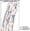 |
Fig. A.1. A sub-region of the first dataset in this study (same as in Fig. 4), showing the facular map determined at disc centre by SO/PHI-HRT and reprojected onto the reference frame of SDO/HMI. After re-projection, an additional selection criterion is applied: only those facular pixels are kept, for which the reprojected BLOS/μ, originally measured at disc centre, exceeds three times the noise level of SDO/HMI at the limb. Pixels meeting this criterion are shown in colour B, while those excluded from the analysis are shown in colour C. |
Appendix B: Approaching the limb
Profiting from the double view-point, we aim to analyse data closer to the limb than previous studies did – which typically consider pixels with μ > 0.1. There are two important considerations in this regard: (1) how close are these pixels to the solar limb; and (2) how well can we reconstruct the centre-to-limb variation of the intensity in these pixels.
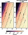 |
Fig. B.1. Close-up of SDO/HMI continuum intensity pixels near the solar limb. Left: Continuum intensity from the hmi.Ic_45s data product, normalised to the mean intensity at disc centre. Right: Corresponding normalised intensity after PSF deconvolution, from the hmi.Ic_45s_dcon data product. The associated μ values are computed from the metadata of the hmi.Ic_45s data product. The solid line marks the solar limb; dashed lines indicate the outermost bin-width (used in Fig. 6); and the dotted line shows the μ = 0.1 contour for reference. |
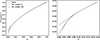 |
Fig. B.2. The centre-to-limb variation (CLV) of the quiet Sun intensity in the first hmi.Ic_45s data set used in the study, along with fifth- and twentieth-order polynomial fits. The left panel shows the full solar disc, while the right panel zooms in on the range 0 < μ < 0.2. |
In this study, we analyse data as close to the limb as μ = 0.05. The first bin in Fig. 6 includes pixels with 0.05 ≤ μ < 0.08. Figure B.1 shows where these pixels fall in relation to the solar limb, and in relation to the more traditional μ > 0.1 approach. The colour scheme shows the Ic at the SDO/HMI limb, for both the hmi.Ic_45s data product and its PSF deconvolved counterpart, the hmi.Ic_45s_dcon. The points considered in our analysis are all at least two pixels away from the solar limb – we consider the solar limb to be where it is defined in the metadata of the SDO/HMI data products. This region also avoids the pixels where the PSF clearly has a very strong influence (which is the case for the closest one to two pixels to the limb).
The use of the hmi.Ic_45s data product has the drawback that centre-to-limb variation (CLV) corrected continuum intensity data are not provided. Previous studies (e.g., Albert et al. 2023; Yeo et al. 2013) apply a fifth-order polynomial fit to the CLV of the quiet sun intensity, following the method of Neckel & Labs (1994), considering only points with μ > 0.1 in their analyses.
However, in the present study we derive facular intensity curves as close to the limb as μ < 0.05. Since the intensity contrast of magnetic elements is defined in relation to the local μ-dependent mean quiet Sun intensity, the accurate determination of this reference is fundamental to our analysis. We have, therefore, evaluated the accuracy to which this relationship is determined, with special focus on the regions near the extreme limb.
Figure B.2 shows the mean quiet Sun intensity as a function of μ for the first SDO/HMI data set used in the study (gray). The mean quiet Sun intensity is derived from pixels with BLOS/< 2 * σ, as a conservative threshold, where σ is the noise level of the SDO/HMI BLOS, determined as a function of μ (see also Sec. 2.5). These pixels are sorted by their associated μ values and grouped into bins of 5000 pixels each, for which the mean is calculated. We then fit the resulting profile with both a fifth-order and a twentieth-order polynomial (green and red, respectively).
The fifth-order fit overestimates the intensity for μ < 0.08, causing an artificial decrease in the derived intensity contrast in this region. Although the sudden intensity drop in the CLV profile is likely instrumental, using a higher-order polynomial substantially improves the fit. For this study, we adopt the twentieth-order polynomial, which provides a very good match down to μ ≈ 0.035, as shown in Fig. B.2. This allows us to confidently include points with μ > 0.05 in our analysis.
Appendix C: Differences between the results from a single and double view-points
For additional insight, we present an intermediate step between the green and orange curves in Fig. 6. Figure C.1 shows three curves: the green curve is the same as the one in Fig. 6, while the orange curve is from SDO/HMI-data only, however it is restricted to the region which is seen by both SDO/HMI and SO/PHI, instead of using data from the full solar disc (as in Fig. 6). The intermediate curve, in blue, is calculated based on pixels identified as faculae at the disc centre, while retaining the BLOS/μ values measured at the limb (consistent with the single-viewpoint approach). See also the legend in Fig. C.1 for an overview of the differences between the curves.
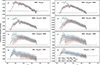 |
Fig. C.1. Same relationship as shown in Fig. 6, but limited to data in the common field-of-view of SDO/HMI and SO/PHI, which falls between 0.05 < μ < 0.75. Consequently, the orange curve now uses much less data than that shown in Fig. 6, and therefore has more limited statistics, but it is calculated in the same way as the one in Fig. 6. The green curve (double-viewpoint approach) remains unchanged. An additional blue curve is included, representing the facular contrast derived from both Ic and BLOS measured at the limb, but using pixels selected from the facular map derived at disc centre. Markers and shaded areas have the same meaning as in Fig. 6. |
We can now examine the differences and agreements between these curves. First, we focus on the comparison of the orange and blue curves, which represent, respectively, the purely single-viewpoint data and the data where the facular map is derived from the disc-centre perspective. As expected from the increase of noise and decrease of resolution at the limb, most of the additional pixels identified by the new facular map correspond to low magnetic field strengths (see also Sec. 2.5). This improved identification of faculae near disc centre effectively extends the curve closer to the limb for the lowest magnetic field categories (panels f to h).
Faculae with stronger magnetic field are identified in both viewpoints, and as a result the blue and orange curves are close in panels a to d. However, in panel a, while the orange curve extends all the way to μ = 0.05, the blue curve stops at μ = 0.11. This suggests that at the extreme limb, the single-viewpoint identification introduces several high-magnetic-field pixels that do not correspond to faculae. These may result from measurement noise, amplified by the division by μ, or from strong Stokes V signals produced by horizontal magnetic fields in the quiet Sun.
Second, we examine how the results change when incorporating disc-centre information about the magnetic field. We compare the blue and green curves: the blue curve uses the facular map from disc centre but retains BLOS values from the limb, while the green curve uses both the facular map and magnetic field values from disc-centre observations. In this comparison, a key consideration is the reclassification of pixels into different magnetic field categories, as changes in BLOS/μ can shift pixels between panels. These changes can be interpreted in terms of change in the contrast curves, under the general assumption that faculae associated with stronger magnetic fields tend to exhibit higher contrasts.
For example, in panel (h) of Fig. C.1, the polarity reversal line (see Fig. 10) appears as a peak in the contrast in the blue curve just below μ = 0.2. It is the results of high-intensity pixels near the solar limb being incorrectly assigned very low magnetic field values. When these pixels are reassigned to the correct magnetic field categories using disc-centre information, this contrast enhancement disappears in the green curve. In panel (g), which also represents low magnetic fields, the blue and green curves remain in good agreement. This suggests that although some pixel exchange between magnetic field categories occurs, the majority of the contributing pixels are newly introduced and are associated with low magnetic fields at the limb as well.
At higher magnetic field strengths (panels a to f), the contrast in each category increases when using disc-centre information. This trend reflects the general overestimation of BLOS/μ near the limb, as discussed in Sec.3.1, and illustrated in Fig.10. After correction, pixels that were previously misclassified into higher field categories move into lower ones; and in panel a, no pixels remain below μ = 0.23. This re-sorting also increases the mean intensity contrast: in the high-field categories by removing lower-contrast, misclassified pixels, and in the lower-field panels by correctly adding higher-contrast pixels.
All Figures
|
Fig. 1. Sketch of observing geometry between Solar Dynamics Observatory (SDO) and Solar Orbiter for observations used in the study. The coordinate system is with the Earth and the Sun at fixed positions, as seen from above. While SDO observes the Sun from the Earth’s perspective, on the horizontal black line, the Solar Orbiter varies its view angle between the two red lines, moving from right to left (i.e. approaching the Sun-Earth line). The spacecraft illustrations are provided courtesy of ESA and NASA. |
| In the text | |
|
Fig. 2. First and last dataset pairs used in this study, from 20 and 22 October 2022 (A and B, respectively). Top: BLOS and μ of a facular region near disc centre (a and b). Bottom: BLOS and μ of same region, as seen simultaneously by SDO/HMI (c and d). The contour shows the location of the SO/PHI field of view, and the μ in the SDO/HMI view-point is shown only for the contoured region. |
| In the text | |
|
Fig. 3. Co-observation of BLOS in same region at the limb (SDO/HMI, left) and at disc centre (SO/PHI-HRT, right), from the first dataset pair in our study. The SO/PHI observation time was 2022-10-20T21:15:46, which corresponds to 2022-10-20T21:20:28 at Earth after accounting for light travel time (in UTC). The SDO/HMI observation time was 2022-10-20T21:19:58 UTC. |
| In the text | |
|
Fig. 4. Sub-region of first dataset pair in time series used in the study, showing BLOS derived from the limb observation by SDO/HMI (first panel), the same data divided by μ (BLOS/μ, second panel), and BLOS derived from disc centre by SO/PHI-HRT; these are divided by the μ value of the disc-centre view and re-projected to the limb to match the reference frame of SDO/HMI (third panel). |
| In the text | |
|
Fig. 5. Data combined in our analysis from different viewing angles. Left: BLOS derived at disc centre from SO/PHI-HRT observations, normalised by the local μ at which it was observed and reprojected to the limb. Right: Intensity contrast is computed from SDO/HMI Ic data at the limb. Contours: We identified facular pixels at disc centre in SO/PHI-HRT observations and then re-projected this map to the limb. The same sub-region as in Fig. 4 is shown. |
| In the text | |
|
Fig. 6. Relationship between facular intensity contrast and μ. Panels (a)–(h) show pixels grouped by their associated BLOS/μ values. Points represent the mean intensity contrast in μ bins of width 0.03; shaded areas indicate the standard deviation within each bin. Orange dots correspond to a single-viewpoint analysis using SDO/HMI data from the full disc. Green triangles represent results from the dual-viewpoint approach, combining SO/PHI-HRT observations at the disc centre with SDO/HMI observations near the limb in the region of overlap. Note that the y-axis limits differ between panels. |
| In the text | |
|
Fig. 7. Number of pixels averaged in each μ bin for the results in Fig. 6. The y-axis is labelled from ‘a’ to ‘h’ in accordance with the panel identifiers in Fig. 6. Top panel: Single-viewpoint case (orange dots in Fig. 6). Bottom panel: Double-viewpoint case (green triangles in Fig. 6). A logarithmic colour scale is used. Note that the single-viewpoint analysis has more pixels overall, as we consider the entire solar disc, as opposed to the small, overlapping field-of-view region in the double viewpoint. |
| In the text | |
|
Fig. 8. Differences in faculae identification between direct limb observations (as in state-of-the-art studies) and identifications performed on disc-centre data, with the results re-projected to the limb (this study). Colour B shows facular pixels identified both at the disc centre and at the limb, while colour C shows the faculae missed at the limb compared to the disc-centre view. Colour D shows pixels identified as faculae in the limb data, which do not appear as faculae at the disc centre. The same sub-region and dataset pair as in Fig. 4 is shown. |
| In the text | |
|
Fig. 9. Intensity contrast of a facular region at the limb. Left: Facular pixels are identified at the limb. Right: Facular pixels are identified at the disc centre. Bottom: Histogram of pixels in the top left and right panels. We show a sub-region of the first dataset in the study, corresponding to μ < 0.2. |
| In the text | |
|
Fig. 10. Sub-region of the first dataset pair in the study, illustrating the change in BLOS category of facular pixels between vantage points. Left: Limb view. Right: Disc-centre view. The categories (a to h in Fig. C.1) are assigned colours ranging from blue to yellow, which are used to colour the pixels in the images. Same region as in Figure 9. |
| In the text | |
|
Fig. A.1. A sub-region of the first dataset in this study (same as in Fig. 4), showing the facular map determined at disc centre by SO/PHI-HRT and reprojected onto the reference frame of SDO/HMI. After re-projection, an additional selection criterion is applied: only those facular pixels are kept, for which the reprojected BLOS/μ, originally measured at disc centre, exceeds three times the noise level of SDO/HMI at the limb. Pixels meeting this criterion are shown in colour B, while those excluded from the analysis are shown in colour C. |
| In the text | |
|
Fig. B.1. Close-up of SDO/HMI continuum intensity pixels near the solar limb. Left: Continuum intensity from the hmi.Ic_45s data product, normalised to the mean intensity at disc centre. Right: Corresponding normalised intensity after PSF deconvolution, from the hmi.Ic_45s_dcon data product. The associated μ values are computed from the metadata of the hmi.Ic_45s data product. The solid line marks the solar limb; dashed lines indicate the outermost bin-width (used in Fig. 6); and the dotted line shows the μ = 0.1 contour for reference. |
| In the text | |
|
Fig. B.2. The centre-to-limb variation (CLV) of the quiet Sun intensity in the first hmi.Ic_45s data set used in the study, along with fifth- and twentieth-order polynomial fits. The left panel shows the full solar disc, while the right panel zooms in on the range 0 < μ < 0.2. |
| In the text | |
|
Fig. C.1. Same relationship as shown in Fig. 6, but limited to data in the common field-of-view of SDO/HMI and SO/PHI, which falls between 0.05 < μ < 0.75. Consequently, the orange curve now uses much less data than that shown in Fig. 6, and therefore has more limited statistics, but it is calculated in the same way as the one in Fig. 6. The green curve (double-viewpoint approach) remains unchanged. An additional blue curve is included, representing the facular contrast derived from both Ic and BLOS measured at the limb, but using pixels selected from the facular map derived at disc centre. Markers and shaded areas have the same meaning as in Fig. 6. |
| In the text | |
Current usage metrics show cumulative count of Article Views (full-text article views including HTML views, PDF and ePub downloads, according to the available data) and Abstracts Views on Vision4Press platform.
Data correspond to usage on the plateform after 2015. The current usage metrics is available 48-96 hours after online publication and is updated daily on week days.
Initial download of the metrics may take a while.