| Issue |
A&A
Volume 706, February 2026
|
|
|---|---|---|
| Article Number | A176 | |
| Number of page(s) | 18 | |
| Section | Extragalactic astronomy | |
| DOI | https://doi.org/10.1051/0004-6361/202557795 | |
| Published online | 10 February 2026 | |
HALO
I. Photometric continuum reverberation mapping of Fairall 9
1
Center for Theoretical Physics, Polish Academy of Sciences Al. Lotników 32/46 02-668 Warsaw, Poland
2
Astroinformatics, Heidelberg Institute for Theoretical Studies Schloss-Wolfsbrunnenweg 35 69118 Heidelberg, Germany
3
Institut d’Astrophysique et de Géophysique Université de Liège Allée du six août 19c B-4000 Liège (Sart-Tilman), Belgium
4
International Gemini Observatory/NSF NOIRLab Casilla 603 La Serena, Chile
5
Nicolaus Copernicus Astronomical Center, Polish Academy of Sciences Bartycka 18 00-716 Warszawa, Poland
6
Universidad de Concepción, Departamento de Astronomía Casilla 160 – C Concepción, Chile
7
Aryabhatta Research Institute of Observational Sciences Nainital 263001 Uttarakhand, India
8
c/o Tracy L. Turner 205 South Prospect Street Granville OH 43023, USA
9
Department of Theoretical Physics and Astrophysics, Faculty of Science, Masaryk University Kotlářská 2 611 37 Brno, Czech Republic
10
Astronomical Institute of the Czech Academy of Sciences Boční II 1401 CZ-14100 Prague, Czech Republic
11
Institute of Astronomy, Faculty of Physics, Astronomy and Informatics, Nicolaus Copernicus University ul. Grudziądzka 5 87-100 Toruń, Poland
12
Millenium Institute of Astrophysics Avenue Libertador Bernardo O’Higgins 340 Casa Central Santiago, Chile
13
LIRA, Observatoire de Paris, Université PSL, Sorbonne Université, Université Paris Cité, CY Cergy Paris Université, CNRS 92190 Meudon, France
14
French-Chilean Laboratory for Astronomy, IRL 3386, CNRS and U. de Chile Casilla 36-D Santiago, Chile
15
Department of Applied Physics/Physics, Mahatma Jyotiba Phule Rohilkhand University Bareilly 243006, India
★ Corresponding authors: This email address is being protected from spambots. You need JavaScript enabled to view it.
; This email address is being protected from spambots. You need JavaScript enabled to view it.
; This email address is being protected from spambots. You need JavaScript enabled to view it.
Received:
22
October
2025
Accepted:
14
December
2025
Abstract
Context. We investigate the origin of inter-band continuum time delays in active galactic nuclei (AGNs) in order to study the structure and properties of their accretion disks.
Aims. We aim to measure the inter-band continuum time delays through photometric monitoring of Seyfert galaxy Fairall 9 to construct the lag-spectrum. Additionally, we explain the observed features in the Fairall 9 lag-spectrum and discuss the potential drivers behind them based on our newly collected data from the Obserwatorium Cerro Murphy (OCM) telescope.
Methods. We initiated a long-term, continuous AGN photometric monitoring program in 2024 titled Hubble constant constraints through AGN Light curve Observations (HALO) using intermediate and broadband filters. Here, we present the first results from HALO, focusing on photometric light curves and continuum time-delay measurements for Fairall 9. To complement these observations and extend the wavelength coverage of the lag-spectrum, we also reanalyzed archival Swift light curves and spectroscopic data available in the literature.
Results. Using HALO and Swift light curves, we measured inter-band continuum delays to construct the lag-spectrum of Fairall 9. Excess lags appear in the u and U bands (Balmer continuum contamination) and in the I band (Paschen jump and dust emission from the torus). Overall, the lag-spectrum deviates significantly from standard disk model predictions.
Conclusions. We find that inter-band delays deviate from the power law, τλ ∝ λβ, due to broad-line region scattering, reprocessing, and dust contributions at longer wavelengths. Power-law fits are therefore not well suited to characterizing the nature of the time delays.
Key words: galaxies: active / galaxies: distances and redshifts / galaxies: nuclei / galaxies: photometry / quasars: emission lines / galaxies: Seyfert
Gemini Science Fellow.
Retired.
© The Authors 2026
 Open Access article, published by EDP Sciences, under the terms of the Creative Commons Attribution License (https://creativecommons.org/licenses/by/4.0), which permits unrestricted use, distribution, and reproduction in any medium, provided the original work is properly cited.
This article is published in open access under the Subscribe to Open model. This email address is being protected from spambots. You need JavaScript enabled to view it. to support open access publication.
1. Introduction
In active galactic nuclei (AGNs), which are among the most luminous objects in the Universe, matter accretes onto a central supermassive black hole (SMBH) and forms an optically thick and geometrically thin standard accretion disk (SSD; Shakura & Sunyaev 1973). According to the lamp-post model (George et al. 1989; Matt et al. 1991), the disk of an AGN is illuminated by a compact ionizing X-ray source. The intercepted radiation is subsequently reprocessed into UV–optical emission, with progressively larger disk radii contributing to longer wavelengths as the disk temperature decreases outward, following the relation  (Collier et al. 1999).
To probe the structure of such accretion disks, several studies have employed photometric continuum reverberation mapping (continuum-RM; Sergeev et al. 2005; McHardy et al. 2014; Shappee et al. 2014; Jiang et al. 2017; Mudd et al. 2018; Homayouni et al. 2019; Yu et al. 2020; Dalla Bontà et al. 2020; Kara et al. 2021; Jha et al. 2022; Guo et al. 2022; Kara et al. 2023; Sharp et al. 2024; Edelson et al. 2024; Mandal et al. 2025; Prince et al. 2025; Pozo Nuñez et al. 2025), and their investigations have revealed several key outcomes. First, inter-band time delays are broadly found to follow a power-law dependence on wavelength, τλ ∝ λβ, with a slope of β ∼ 4/3 (Kara et al. 2021; Guo et al. 2022; Kara et al. 2023; Mandal et al. 2025), in good agreement with the predictions of the SSD model. This consistency now extends even to the highest redshift probed through continuum-RM (z = 2.7; Pozo Nuñez et al. 2025). Nevertheless, a number of continuum-RM studies have reported accretion-disk sizes and wavelength-delay slopes that deviate from the SSD prediction (e.g., Fausnaugh et al. 2016; Starkey et al. 2017; Lawther et al. 2018; Fian et al. 2023b; McHardy et al. 2023), suggesting that the structure and reprocessing properties of some AGN disks may be more complex than assumed in the simple model. Second, the continuum-emitting region size inferred from SSD-based power-law fits is consistently measured to be about three to five times larger than predicted, a discrepancy often referred to as the “disk-size anomaly” (Fausnaugh et al. 2016; Kara et al. 2023; Mandal et al. 2025). This mismatch is now thought to arise from contamination due to broad-line region (BLR) scattering and reprocessing, which can increase the UV–optical time delays (Korista & Goad 2001; Netzer 2022). Alternatively, as discussed by Kammoun et al. (2021a,b, 2023), an enlarged disk size at a given wavelength can arise from the significant vertical extent of the X-ray corona. Interestingly, these continuum-emitting sizes also show correlations with AGN luminosity and BLR sizes, suggesting that continuum time delays measured from photometric light curves may provide a promising avenue for black hole mass measurements once established over a large dynamic range in luminosity (Wang et al. 2023; Panda et al. 2024; Mandal et al. 2025). Third, observed lag-spectra reveal a significant excess lag around the 3646 Å Balmer jump (Cackett et al. 2018), with an additional potential excess around the 8206 Å Paschen jump (Guo et al. 2022). These excess lags strongly indicate contamination from the BLR, causing the inter-band time delays to deviate significantly from a simple power-law wavelength dependence.
Recently, we have demonstrated that photometric continuum time delays provide a powerful method for estimating the Hubble constant (H0) by simultaneously fitting the lag-spectrum and the spectral energy distribution (SED) of AGNs (see Jaiswal et al. 2025, for details). Our study, based on the well-studied AGN NGC 5548, yielded an H0 estimate of  km s−1 Mpc−1 with an uncertainty of about 10–15%. Although this error is relatively large and derived from a single object, the approach shows great promise, i.e., by extending such measurements to a large sample of AGNs spanning a wide range of redshifts, the uncertainty can be significantly reduced, thereby offering a new avenue to address the ongoing Hubble tension (Abdalla et al. 2022).
Motivated by this potential, we initiated a long-term AGN photometric monitoring program at the Rolf Chini Cerro Murphy Observatory (OCM, from Polish: Obserwatorium Cerro Murphy) 60 cm telescope in Chile, namely, Hubble constant constraint through AGN Light curves Observation (HALO). The HALO program began in 2024 and employs multifilter photometry using the Strömgren u, v, b, y, and Johnson–Cousins I bands to probe continuum time delays. As part of HALO, we have completed observations of one target, the bright Seyfert galaxy Fairall 9.
Fairall 9 is a well-known and extensively studied AGN. It was first identified during a survey for galaxies with bright compact nuclei in the southern sky (Fairall 1977), and it soon attracted attention because of its relative brightness and proximity, with a redshift of z = 0.046145. Over the years, multiwavelength observations spanning the X-ray, ultraviolet, optical, and infrared bands have provided a comprehensive characterization of its physical properties. In particular, X-ray spectral studies have shown that Fairall 9 is relatively simple in structure, often classified as a ‘bare AGN’ since it lacks the strong warm absorbers commonly detected in many other Seyfert galaxies (Patrick et al. 2011; Emmanoulopoulos et al. 2011). Its intrinsic variability has further established it as a valuable target for long-term monitoring, motivating extensive campaigns that have been conducted over several decades (e.g., Rodríguez-Pascual et al. 1997; Peterson et al. 1998). Most notably, Edelson et al. (2024) reported the results of an exceptionally dense 1.8-year daily monitoring program with Swift, whereas Hernández Santisteban et al. (2020) analyzed the first year of the same campaign while complementing it with ground-based observations. These studies serve as an invaluable reference for our work, enabling a comparison between space-based and ground-based monitoring approaches.
In this paper, we present our optical photometric monitoring of Fairall 9 using four Strömgren and one Johnson-Cousins filters. Our current analysis focuses on constructing the lag-spectrum of this source, which will form the basis for subsequent estimation of H0 within the broader HALO framework. The paper is organized as follows: In Sect. 2 we outline the observations and data reduction procedures. Section 3 provides details regarding the flux variability, host-galaxy flux estimation, and time-series analysis. The results are presented in Sect. 4 and followed by a discussion in Sect. 5. Finally, Sect. 6 provides a summary of the main findings.
2. Observations and data reduction
The core objective of HALO is to perform simultaneous modeling of inter-band continuum time delays and SEDs for a well-selected sample of AGNs across a broad luminosity and redshift range. Observations for this project are primarily conducted using meter-class robotic telescopes at the OCM, an international astrophysical project, hosted in European Southern Observatory (ESO) in Chile, and operated by the Nicolaus Copernicus Astronomical Center of the Polish Academy of Sciences in Warsaw, Poland. A detailed overview of the HALO project will be presented in Pozo Núñez et al. (in prep.). Below, we describe the photometric monitoring campaign targeting Fairall 9.
2.1. Observations
The monitoring was conducted between September 20, 2024, and February 17, 2025, using the Strömgren u, v, b, and y filters to trace the AGN’s optical continuum in spectral regions minimally affected by emission lines. To extend coverage toward the red end of the optical spectrum, the Johnson-Cousins I filter was also used. The main properties of Fairall 9 are summarized in Table 1.
Basic properties of Fairall 9.
To ensure that our photometric measurements are free from contamination by broad emission lines, we carefully selected four Strömgren intermediate-band filters along with the Johnson-Cousins I filter. This selection was made specifically to minimize contamination from any prominent broad emission features within the filter bandpasses. In contrast to many previous continuum–RM studies, which often lacked this level of precision in filter selection, our approach prioritizes minimizing contamination from the BLR while maximizing the contribution from the underlying accretion disk continuum. We illustrate the chosen filter transmission curves in Figure 1 overlaid on the optical spectrum of Fairall 9 (Edelson et al. 2024). This approach provides an optimal framework to evaluate the consistency of our observations with predictions from the standard disk model and to explain the disk size anomalies reported in earlier studies.
 |
Fig. 1. Ultraviolet and optical spectra of Fairall 9 obtained with the HST Faint Object Spectrograph on 1993 January 21 and with the ESO 1.5 m telescope on 1994 July 14, respectively. Overplotted are the transmission curves of the OCM filters (u, v, b, y, and I) used for photometric observations in our HALO program, along with the transmission curves of Swift-UVOT filters (W2, M2, W1, U, B, and V) employed in constructing the photometric light curves in the literature. |
2.2. Data reduction
For photometric data reduction, we followed standard procedures, including bias subtraction, dark current removal, flat-fielding, astrometric calibration, and distortion correction. These steps were carried out using a combination of standard IRAF1 (Tody 1986) tasks and custom-developed routines, following the detailed methodology described in Pozo Nuñez et al. (2017).
The light curves were then extracted using aperture photometry. To optimize the signal-to-noise ratio (S/N) and minimize flux scatter, photometry was first performed on all stars in the field across a range of aperture sizes. From these measurements, a photometric curve of growth was constructed using the instrumental magnitudes at different apertures to evaluate the combined contributions from the host galaxy and the central engine of Fairall 9. Field stars were subsequently selected according to brightness, proximity to the AGN, and the standard deviation (σ*) of their light curves.
Small apertures (1.0–2.0 arcsec) yielded higher scatter due to PSF sensitivity and incomplete flux inclusion, while large apertures (15–20 arcsec) increased σ* as a result of elevated background contamination. In general, σ* was found to be brightness-dependent. To ensure photometric stability, we selected reference stars with brightness levels similar to the AGN and located within 25 arcminutes of the target. From these, the top 20% with the lowest σ* values were retained, yielding a final set of 12 reference stars. Subsequently, relative light curves were constructed by normalizing the AGN flux to the ensemble of selected reference stars. The final AGN light curve corresponds to the average flux calibrated against this reference set.
The absolute flux calibration was performed using non-variable stars flagged for high quality in the DES Data Release 2 catalog (Abbott et al. 2021), located in the same field as Fairall 9. The calibration accounts for both atmospheric extinction (Patat et al. 2011) and Galactic foreground extinction. The latter was derived from the Schlafly & Finkbeiner (2011) recalibration of the dust maps by Schlegel et al. (1998), using NED2 extinction values at the source coordinates with E(B − V) = 0.023. These values were interpolated to the effective wavelengths of our filters. The final light curve data in u, v, b, y, and I bands are provided in Table 2.
Photometric light curve data from HALO.
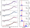 |
Fig. 2. Light curves from OCM monitoring and lag analysis. Left: Light curves of Fairall 9 in the u, v, b, y, and I filters, shown from top to bottom, respectively. In each panel, the dashed lines in various colors indicate second-order polynomial detrending, while the solid lines represent the best-fit light curves obtained from PyROA. The full light curve is divided into two segments, S1 and S2, separated by an observational gap indicated by the vertical dashed orange line. Right: Distribution of the cross-correlation coefficient relative to the u band (solid black line) derived using the ICCF method for the full, non-detrended original light curve. The blue histogram shows the cross-correlation centroid distribution from ICCF, the red histogram represents the lag probability distribution obtained from PyROA, and the brown histogram shows the corresponding distribution from JAVELIN. A vertical dashed gray line marks the reference point at τ = 0 days. |
2.3. Spectrum data
In addition to our photometric monitoring of Fairall 9, we also compiled spectroscopic data from the literature, as such data are essential for constructing the SED and assessing potential BLR contamination in the measured continuum inter-band delays. Specifically, we incorporated UV spectrum observed with the Hubble Space Telescope (HST) Faint Object Spectrograph obtained on 1993 January 21 (Edelson et al. 2024). Furthermore, an optical spectrum is available from the optical monitoring campaign using the European Southern Observatory (ESO) 1.5 m telescope equipped with the Boller & Chivens spectrograph and a CCD detector (Santos-Lleó et al. 1997), conducted in synergy with the eight-month monitoring campaign using the International Ultraviolet Explorer (IUE; Rodríguez-Pascual et al. 1997).
For our study, we utilized the combined UV and optical spectrum of Fairall 9 which was presented by Edelson et al. (2024). This spectrum is shown in Figure 1.
2.4. Additional photometric data from Swift
We collected additional light curve data of Fairall 9 from the literature. For this purpose, we adopted the homogeneous and relatively uninterrupted set of Swift observations assembled by Edelson et al. (2024), which includes hard- and soft- X-ray light curves from the X-Ray Telescope (XRT) as well as UV-optical light curves in the W2, M2, W1, U, B, and V bands from the Ultraviolet/Optical Telescope (UVOT). We did not include the dataset from Hernández Santisteban et al. (2020), as those Swift observations were already incorporated in the compilation of Edelson et al. (2024). Likewise, we followed Edelson et al. (2024) in excluding data from the Las Cumbres Observatory Global Telescope (LCOGT) network, and used Swift light curve data up to MJD ∼58 900 in order to maintain the homogeneity and uniformity of the light curves.
3. Analysis
3.1. Flux variability
We present the light curves of Fairall 9 in Figure 2 in the u, v, b, y, and I filters. To quantify the flux variability of the source, we computed the normalized excess variance, Fvar (Rodríguez-Pascual et al. 1997; Vaughan et al. 2003), defined as
 (1)
(1)
where ⟨F⟩ is the mean flux over the light curve. The sample variance, σ2, and the mean square measurement uncertainty,  , were calculated as
 (2)
(2)
 (3)
(3)
where ϵi denotes the uncertainty associated with each individual flux measurement. The uncertainties in Fvar were estimated following the methodology described in Edelson et al. (2002) and Mandal et al. (2021). Additionally, we calculated the maximum to minimum flux ratio, defined by the parameter Rmax. The obtained variability properties are summarized in Table 3.
Light curve properties and results from the variability analysis.
In the top panel of Figure 3, we present the SED in optical bands derived from the mean fluxes and their corresponding uncertainties, as obtained from the multiband light curves. All flux measurements were corrected for Galactic extinction. A standard thin accretion disk model predicts an SED that follows the relation λFλ ∝ λ−4/3. To test this, we first fit the observed SED with a power-law function, obtaining λFλ ∝ λ−0.67 ± 0.01. This slope is significantly shallower than the theoretical expectation, indicating a deviation from the standard accretion disk prediction.
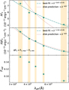 |
Fig. 3. Results from the photometric flux variability analysis. Top: Optical SED of Fairall 9 derived from the mean fluxes in the u, v, b, y, and I filters. Middle: Differential SED constructed from the difference between the maximum and minimum fluxes in the corresponding filters. Bottom: Normalized excess variance, Fvar, as a function of wavelength. In both the top and middle panels, the dot-dashed teal line represents the best-fit power law with a free spectral index, while the dashed brown line corresponds to a power law with the index fixed at −4/3, as predicted by the standard thin accretion disk model. The orange-shaded regions indicate the ±1σ range, representing the wavelength uncertainty of each filter, as quantified by the rms width of its transmission curve. |
To better isolate the variable component of the emission, we constructed an alternative SED using the difference between the maximum and minimum flux states (ΔFλ) of the light curves (also see; Fausnaugh et al. 2016). This difference SED, shown in the middle panel of Figure 3, provides a more accurate representation of the intrinsic variability of the accretion disk while effectively minimizing contamination from host galaxy starlight in different filters. Fitting this differential SED yields a steeper slope of λFλ ∝ λ−1.52 ± 0.05, which is in much closer agreement with the −4/3 slope predicted by the thin disk model. For reference, we also overplot the theoretical SED slope of −4/3 on both panels by fixing the normalization constant accordingly. This facilitates a direct visual comparison between the observed trends and the canonical thin accretion disk expectation.
In the bottom panel of Figure 3, we show Fvar as a function of wavelength. Across all five filters used in this study, we observe significant flux variability, with Fvar values ranging from 0.0868 to 0.1542. Notably, Fvar shows a gradual decrease with increasing wavelength in Fairall 9, consistent with the commonly observed “bluer when brighter” trend in AGNs (Sakata et al. 2010). However, this decreasing trend flattens at longer wavelengths, suggesting increased contamination from host galaxy starlight, which effectively dilutes the observed variability in those bands (also see Section 3.2 for host-galaxy subtraction). Furthermore, the outer regions of the accretion disk, which emit primarily at optical and near-infrared wavelengths, act as a low-pass filter due to their longer dynamical and thermal timescales. This filtering smooths out rapid fluctuations, thereby reducing the amplitude of variability. As a result, the observed Fvar is both diluted and damped at longer wavelengths.
3.2. Host subtracted AGN luminosity
To estimate the contribution of the host galaxy and isolate the AGN emission, we applied the flux variation gradient (FVG) method as described in Pozo Nuñez et al. (2012). In essence, the method assumes that, for a fixed photometric aperture, flux measurements in different filters are the sum of a variable AGN component and a constant host-galaxy component, the latter including emission from the narrow-line region. Although the AGN flux varies over time, its optical spectral shape remains effectively constant. Consequently, fluxes measured in two bands define a linear relation in flux–flux space, where the slope corresponds to the AGN color and the host galaxy color is confined to a well-defined range (e.g., Sakata et al. 2010). The intersection of the AGN slope with the host-galaxy color range then yields the host flux in each band for the period of monitoring.
Because light curves are affected by photometric noise, we estimated the intersection region using the density of possible solutions from a Bayesian principal component analysis (Gianniotis et al. 2022). Figure A.1 in Appendix A shows the FVG diagrams for all filter pairs, along with the adopted host-galaxy color ranges from Sakata et al. (2010). The resulting median values of AGN, and host-galaxy fluxes for each filter are listed in Table 3.
Our results show that the fractional contribution of the host galaxy increases steadily with wavelength, in agreement with expectations for stellar-dominated emission at longer wavelengths. In the bluest u band, the host accounts for only ∼7% of the total flux, rising to ∼14% in v and ∼22% in b. Beyond 5000 Å, the host fraction becomes more significant, reaching ∼35% in y and nearly 40% in the I band (see Table 3). This wavelength dependence reflects the increasing prominence of the old stellar population in the host galaxy, whose SED peaks in the optical–NIR, while the AGN continuum remains comparatively blue. Accurate host subtraction is therefore particularly critical in the redder filters, where stellar contamination can dominate the flux budget.
Figure 4 presents the median SED after decomposing the total flux into AGN and host-galaxy components using the FVG method. When compared with an Sb galaxy template scaled to the inferred host fluxes, the host contribution shows close agreement across the optical bands. Although Bentz et al. (2009) reported an SBa-type morphology for Fairall 9, our results favor an intermediate-type spiral stellar population as the dominant contributor to its host galaxy. The I-band point lies modestly below the Sb template prediction. Given the low photometric uncertainties and the consistent extraction aperture across all bands, this offset is unlikely to be due to measurement or calibration effects.
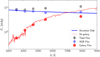 |
Fig. 4. Spectral flux decomposition obtained with the FVG method. Black circles show the total flux density Fν. The host-subtracted AGN spectrum (blue circles) follows the thin accretion-disk prediction Fν ∝ ν1/3 (Shakura & Sunyaev 1973). The host component inferred from the FVG (red stars) is well matched by an Sb galaxy template (red curve; Kinney et al. 1996). |
A more plausible explanation is that the host stellar population differs slightly from that of a canonical Sb galaxy, with a reduced contribution from late-type giants, leading to a lower near-infrared flux. This is consistent with the morphological classification suggested by Jiang et al. (2021) who, from visual inspection of the Hubble ACS image presented by Bentz et al. (2009), proposed a likely SB0/a type. Such an intermediate morphology could produce an SED broadly similar to Sb in the optical while exhibiting reduced flux at longer wavelengths. Nevertheless, the consistency between the difference SED shown in Figure 3 and the host-subtracted SED presented in Figure 4 with the thin accretion disk prediction further supports the reliability of our flux decomposition based on the FVG method.
3.3. Detrending of light curves
In addition to the rapid variations associated with short-timescale accretion disk reverberation, the observed UV-optical light curves also exhibit slower variability on longer timescales. These longer timescales are related to two separate phenomena. The first is the stochastic, multiscale variability of the accretion rate in the innermost regions of the flow (e.g., Vaughan et al. 2003), most likely arising from local fluctuations that propagate inward (Lyubarskii 1997). Such variability can give rise to long-timescale negative delays, which have now been tentatively identified in some sources (e.g., Secunda et al. 2023, specifically in Fairall 9). The second phenomenon is the contribution of reprocessing from more distant regions such as the BLR, and torus, which leads to positive time delays. To isolate the rapid variability and recover short lags, a detrending method is often applied by subtracting the slower variability component from the observed UV-optical light curves (Denney et al. 2010; Li et al. 2018; McHardy et al. 2018; Rakshit 2020; Zajaček et al. 2020; Woo et al. 2024; Edelson et al. 2024; Zajaček et al. 2024). For instance, Edelson et al. (2024) detrended their light curves by fitting and subtracting a second-order polynomial, thereby removing long-term trends.
Following this approach, we adopted the methodology of Edelson et al. (2024) for detrending our light curves. Specifically, we fit the entire light curves with polynomials of order 0, 1, and 2, where order = 0 corresponds to the original, unmodified light curves. We did not employ polynomial orders higher than 2, since higher-order detrending risks oversubtracting genuine short-timescale variability (Edelson et al. 2024) and introducing spurious artifacts into the light curves.
In our subsequent analysis, we therefore made use of both the original and detrended light curves. We emphasize, however, that there is no universally accepted choice for the polynomial order in detrending, and in all cases this process carries the risk of generating artificial variability in the light curves (for more details see the discussion in Appendix B and Figure B.1). For this reason, we treat the original light curves as our primary dataset, while using the detrended versions only for comparison.
3.4. Lag analysis
During our monitoring period, Fairall 9 exhibited correlated significant flux variations across all the five filters used. Therefore, to measure the inter-band time delays, we employed the interpolated cross-correlation function (ICCF) method as our primary analysis tool, implemented via the PyCCF python package (Gaskell & Sparke 1986; Gaskell & Peterson 1987; Peterson et al. 1998; Sun et al. 2018). This method involves linearly interpolating the two light curves and computing the cross-correlation coefficient (r). The uncertainties are estimated using a model-independent Monte Carlo simulation based on flux randomization and random subset selection method following Peterson et al. (1998), Wandel et al. (1999), and Peterson et al. (2004). We repeated the simulation for 5000 iterations, with the lag centroid calculated in each iteration. Subsequently, these centroids were used to construct the cross-correlation centroid distribution (CCCD). For each iteration, the centroid lag was determined using only the points above 80% of the peak value of the cross-correlation function (rmax). The final lag value was obtained from the median of the CCCD, while the associated uncertainties were defined by the 15.9th and 84.1st percentiles of the distribution corresponding to a 1σ confidence interval assuming a Gaussian distribution. We used the u band as the reference light curve, as it corresponds to the shortest wavelength in our monitoring program, and measured the inter-band delays between u versus v (τuv), u versus b (τub), u versus y (τuy), and u versus I (τuI).
In addition to the ICCF method, we also employed PyROA (Donnan et al. 2021) and JAVELIN (Zu et al. 2011) to measure inter-band time delays as a consistency check. PyROA models AGN light curve variability using the running optimal average (ROA) technique, where model parameters are sampled via Markov chain Monte Carlo (MCMC) methods. This empirical approach does not rely on the commonly assumed damped random walk (DRW; Kelly et al. 2009; MacLeod et al. 2010) model. The effective number of parameters in the ROA model is governed by the shape and width (Δ) of its window function, as well as by the sampling cadence and precision of the data. This setup allows for a Bayesian optimization of the ROA width and other parameters, using Bayesian information criterion minimization and MCMC sampling (Donnan et al. 2021). Ultimately, PyROA provides an estimate of the time delay between light curves at different wavelengths.
JAVELIN models and interpolates AGN light curves using the DRW framework (Zu et al. 2011). First, it fits the reference light curve with a DRW model characterized by two parameters, the variability amplitude (σd) and the time scale of variability (τd). The reprocessed continuum light curve is then generated by convolving this model with a top-hat transfer function. Next, the time lag is estimated by maximizing the likelihood through MCMC sampling, with the final lag taken as the median of the resulting lag probability distribution.
The time delays were derived using three different methods applied to various combinations of light curve data, both with and without detrending. The resulting delays are summarized in Appendix C and presented in Table C.1.
Comparing different methods, we noticed small inconsistencies between the nonparametric, model-independent method ICCF and model-dependent approaches that rely on Bayesian or stochastic modeling based on the DRW process, such as PyROA and JAVELIN. While ICCF tends to yield more conservative uncertainties and remains robust even in the presence of flux error mis-estimates, both PyROA and JAVELIN are more sensitive to the underlying modeling assumptions. These assumptions may not fully capture the true nature of AGN variability, particularly when attempting to model short-timescale fluctuations in light curves that span long temporal baselines.
For instance, PyROA fails to accurately model the short-timescale rapid variations, specifically in the b, y and I light curves (as example see Figure 2 for the period MJD ∼60 675 to 60 715), leading to significant deviations in the inferred lags, τuy and τuI, when compared with those obtained from ICCF. Similar discrepancies are also evident when using JAVELIN. This issue is further supported by earlier studies, such as, Mandal et al. (2025) reported that JAVELIN often fails to recover accurate lag values in the presence of large seasonal gaps in the data, and Wang & Woo (2024) suggested that ICCF offers the most robust lag measurements compared to PyROA and JAVELIN. Furthermore, we compare the lags obtained from these three methods in Figure D.1 and discuss them in detail in Appendix D.
Given these limitations, and despite the larger associated uncertainties, we adopt the lags obtained from ICCF as our final measurements in the subsequent analysis, prioritizing reliability and robustness over potentially underestimated errors from model-dependent methods. Note that the inclusion or exclusion of the single data point at MJD 60573.238, which is separated by a large observational gap in the I light curve, does not affect the derived lags. Therefore, we included all available data points in the I band for our analysis.
4. Results
4.1. Disk-mapping: Traditional method with τλ ∝ λβ
According to the lamp-post model, an X-ray emitting corona illuminates the accretion disk, whose reprocessed UV-optical emission shows delayed responses to variations in the shorter-wavelength continuum. This delay arises from the radial temperature gradient in the disk, T(r)∝r−3/4, as predicted by the standard accretion disk model. Consequently, the size of the standard disk at wavelength λ can be expressed as (Edelson et al. 2017)
![Mathematical equation: $$ \begin{aligned} R_{\lambda ,\mathrm{SSD}} = \left(\chi \frac{\kappa \lambda }{hc}\right)^{4/3} \left[\left(\frac{GM_{\mathrm{BH}}}{8 \pi \sigma }\right) \left(\frac{L_{\mathrm{Edd}}}{\eta c^2}\right) (3+\kappa )\lambda _{\mathrm{Edd}}\right]^{1/3}, \end{aligned} $$](/articles/aa/full_html/2026/02/aa57795-25/aa57795-25-eq9.gif) (4)
(4)
where G is the gravitational constant, MBH the black hole mass, σ the Stefan–Boltzmann constant, LEdd the Eddington luminosity, and λEdd the Eddington ratio. The parameter χ is a scaling factor that accounts for systematic discrepancies in converting the annulus temperature T to a wavelength λ at a characteristic radius. The radiative efficiency is denoted by η, and κ represents the ratio of external to internal disk heating. In this work, we assume η = 0.1 and κ = 1, corresponding to equal contributions from X-ray and viscous heating. We adopt χ = 2.49, consistent with a flux-weighted radius (Edelson et al. 2024), while Wien’s law predicts a larger value of χ = 4.97 (Netzer 2022). Note that there is no standard value of χ, which introduces additional uncertainty in Equation (4).
As a result, the inter-band continuum time delays follow a power-law dependence on wavelength as τλ ∝ λ4/3. Measuring these continuum reverberation lags across different UV–optical bands therefore provides a way to infer the temperature profile of the disk. This technique, referred to as disk-mapping, is implemented by fitting the observed inter-band delays as a function of wavelength using the relation
![Mathematical equation: $$ \begin{aligned} \tau _{\lambda } = \tau _{0} \left[\left(\frac{\lambda }{\lambda _{0}}\right)^{\beta }-\alpha \right], \end{aligned} $$](/articles/aa/full_html/2026/02/aa57795-25/aa57795-25-eq10.gif) (5)
(5)
where λ0 represents the reference-band wavelength, τ0 is the normalization amplitude of the power law lag-spectrum at λ0, and β is the power-law index, which is ∼4/3 as prescribed by the SSD model. The parameter α introduces flexibility by allowing the model lag at λ0 to differ from zero; specifically, α = 1 forces the lag at λ0 to be zero. Hence, the normalization constant τ0 inferred from disk-mapping provides a measure of the accretion disk size at λ0, given by Rλ0 = c × τ0.
Although many studies have reported that inter-band delays broadly follow the expected power-law behavior, τλ ∝ λ4/3 (Guo et al. 2022; Kara et al. 2023; Edelson et al. 2024; Mandal et al. 2025; Pozo Nuñez et al. 2025), significant departures from this relation have also been observed in numerous cases (Fausnaugh et al. 2016; Starkey et al. 2017; Fian et al. 2023b; McHardy et al. 2023; Gonzalez-Buitrago et al. 2025). Furthermore, disk sizes inferred from disk-mapping are typically found to be about 4–5 times (0.69 ± 0.04 dex) larger than those predicted by the standard SSD model, a discrepancy commonly referred to as the ‘disk-size anomaly’ (Cackett et al. 2021; Mandal et al. 2025). Similar disk-size anomalies have also been detected in microlensing studies of gravitationally lensed quasars (Rauch & Blandford 1991; Morgan et al. 2010; Blackburne et al. 2011; Chartas et al. 2016; Li et al. 2019; Vernardos et al. 2024).
4.1.1. For HALO dataset
Motivated by these findings, we first perform disk-mapping on Fairall 9 using data from our HALO program, assuming a power-law dependence of τλ on wavelength λ using Equation (5), with τ0, β, and α as free parameters, in order to examine any potential departure from the SSD-predicted slope. We then repeat the analysis by fixing the slope to βfix = 4/3, as expected from the SSD model, and setting α to 1, thereby forcing the lag to be zero at λ0.
In Figure 5, we present the lag-spectra, i.e., the rest-frame inter-band time delays as a function of rest-frame wavelength, using the complete light curves for three different cases: the original light curves, and detrended light curves of order 1 and order 2, shown in the left, middle, and right panels, respectively. When we treat τ0, β, and α as free parameters, we find that the resulting power-law slope varies significantly, ranging between 0.91 and 2.50 for different data combinations, and thus deviates considerably from the SSD-predicted value of 4/3.
 |
Fig. 5. Examples of lag-spectra based on ICCF lag measurements using the complete light curves for three cases: original (left), detrended with order = 1 (middle), and detrended with order = 2 (right). The ICCF lag measurements (red circles) are shown in the rest-frame as a function of rest-frame wavelength. The dot-dashed red line represents the best-fit to the relation τ ∝ λβ using Equation (5), where τ0, β, and α are free parameters. The dot-dashed black line shows the best-fit with fixed β = 4/3 and α = 1 with only τ0 as a free parameter. Shaded regions indicate the 1σ uncertainties from the fitting. The blue and maroon dashed lines show the respective best-fits derived without including τuI in the lag-spectrum for the cases where all parameters (τ0, β, and α) are free and where β = 4/3 and α = 1 are fixed. Vertical and horizontal dotted lines mark the rest-frame reference wavelength and zero rest-lag, respectively. |
However, the disk sizes inferred from the normalization parameter τ0 at the reference wavelength λ0 cannot be directly compared with the SSD-predicted value, since β deviates significantly from 4/3, and the τ = 0 lags in the best-fit models are shifted relative to the reference wavelength λ0 = 3468.0 Å/(1+z).
When we repeat the analysis by fixing β and α to 4/3 and 1, respectively, leaving only τ0 as a free parameter, we find systematically larger disk sizes, about 1.5–3.6 times greater than the SSD prediction. These results consistently indicate a significant departure from the SSD expectations.
Since the object variability shows an apparent change in the middle of our monitoring (see Figure 2), we also analyzed separately the two segments: S1 and S2, which are divided by an observational gap. The best-fit values obtained from our disk-mapping analysis are summarized in Table 4, where the corresponding χ2 per degree of freedom (χ2/d.o.f.) values are also listed. Among the various disk size measurements derived from different data combinations, the original dataset for S2 and the detrended dataset with order = 1 for S1 provide comparatively better estimates, with χ2/d.o.f. = 0.98 (0.78) and 1.00 (1.25) when β and α are treated as free (fixed) parameters during fitting, respectively. The corresponding disk sizes at λ0 = 3468.0 Å/(1+z) are  light-days for S2-original and
  light-days for S1-detrending = 1.
Parameters estimated from the disk-mapping.
For comparison, Hernández Santisteban et al. (2020) and Edelson et al. (2024) reported disk sizes of R1928 = 1.20 ± 0.10 light-days, and R2050 = 1.81 ± 0.20 light-days at reference wavelengths of 1928 Å and 2050 Å, respectively. When extrapolated to 3315 Å with βfix = 4/3, these correspond to R3315 = 2.47 ± 0.21 light-days, and 3.44 ± 0.38 light-days, respectively. In contrast, our estimated disk sizes are smaller by a factor of ∼2 − 4 compared to those reported by Hernández Santisteban et al. (2020) and Edelson et al. (2024). This discrepancy can arise due to (i) firstly, the inter-band delays do not strictly follow a simple power law; instead, the lag-spectrum exhibits wavelength-dependent wiggles. These features are primarily caused by Balmer continuum contamination in the u (or Swift U, see the following section) band and diffuse continuum emission due to BLR reprocessing across all continuum-tracing filters. Consequently, disk size estimates based on power-law fits may vary between monitoring campaigns, depending on the wavelength coverage. (ii) Secondly, differences in data quality between monitoring periods can further affect the measured lags and, in turn, the resulting lag-spectrum fits. Our observations, obtained with intermediate-band Strömgren filters, benefit from denser sampling (Δt ∼ 0.3 days) and the absence of emission-line contamination, thereby offering a clearer recovery of subtle accretion-disk reverberation signals. In contrast, their campaigns relied on broad-band filters with relatively sparse sampling (Δt ∼ 1.3 days), making them more susceptible to emission-line dilution and less sensitive to small-scale disk variations. And (iii) thirdly, the small variations in disk sizes estimated from different seasons (S1 and S2) of our light-curve observations further suggest that the source may undergo intrinsic changes in the accretion disk-reverberation timescale across epochs.
4.1.2. For combined dataset: HALO plus literature
To further investigate the discrepancies between our lag-spectra fitting of Fairall 9 and the results reported in the literature, we compiled additional light-curve data from the literature. In particular, we made use of the Swift light curves assembled by Edelson et al. (2024) (see Appendix E for details). The resulting delays are summarized in Table E.1 and are hereafter referred to as the “Literature” measurements.
We then plot the inter-band delays obtained from Swift observations together with our HALO measurements in the lag-spectrum shown in Figure 6. We exclude both HX- and SX-band lags from the lag-spectrum, as hard and soft X-rays are generally assumed to originate in the X-ray corona rather than from reprocessed emission in the accretion disk, leading to relatively weak correlations between the X-ray and UV-optical light curves. Remarkably, the lags within the overlapping wavelength range of filters show good consistency between measurements from HALO and those from Literature, despite derived from two independent monitoring programs carried out over distinct time periods. This consistency further suggests that the discrepancy in disk sizes inferred from these separate disk-mapping campaigns is not due to temporal variations or differences in data quality, but rather due to deviations from a simple power-law dependence of lag on wavelength.
 |
Fig. 6. Combined lag–spectrum. Red circular points show our HALO measurements, while black square points indicate reanalyzed literature measurements based on the light curve data from Edelson et al. (2024). The horizontal error bars represent the rms width of the transmission curve as the filter’s wavelength uncertainty. The dot-dashed red and black lines, together with their shaded regions, represent the best-fit results from power-law lag–spectrum fitting, with β and α treated as free parameters and fixed at 4/3 and 1, respectively. The corresponding fits obtained excluding τuI from the lag-spectrum are shown by the dashed blue and maroon lines. The lag–spectrum shows a clear excess in the u and U bands, suggesting Balmer continuum contamination from the BLR in these bands. |
In addition, the combined lag-spectrum of Fairall 9 reveals a pronounced excess in the u and U bands, a feature that points to a significant contribution from the Balmer continuum in these bands. Such an excess has previously been observed in NGC 4593 (Cackett et al. 2018), further supporting this interpretation.
These results highlight that the inter-band delays significantly deviate from the simple power-law trend τλ ∝ λβ. In particular, when using the complete original light curve data, we find negative delays, τuv, τub, and τUB, which suggest a significant Balmer continuum contribution from the BLR to the u and U bands. However, when the light curves are detrended, the Balmer continuum contamination appears to diminish progressively with increasing detrending order. This reduction is likely due to the removal of long-timescale trends, which are expected to originate from the outer regions, such as BLR and/or torus. It should be noted, though, that there is no standard method for such detrending (Edelson et al. 2024) that avoids introducing artifacts into the observed light curves. Nevertheless, the results clearly indicate that the standard thin SSD model alone cannot account for the observed lag-spectra since a simple power-law fit fails to reproduce individual features present in the AGN lag-spectra.
However, τuI deviates significantly from the overall trend, exhibiting an excess lag in the lag-spectrum. This anomaly at the longest wavelength likely arises from contamination by the dust torus and the Paschen jump emission from the BLR (see Section 5.1 for more details). Such excess lag can steepen the power-law slope, thereby affecting the normalization constant τ0. To assess the influence of τuI on the power-law fitting, we refit the lag-spectrum after excluding τuI; the best-fit results are listed in Table 4. For the HALO dataset, the revised fit gives β = 1.83, which is lower than the β = 2.50 obtained from the lag-spectrum including τuI constructed using the original-total light curve data, yet remains steeper than the SSD prediction and is accompanied by a significantly smaller normalization constant. For other data combinations, we find even flatter lag–wavelength dependencies (β ∼ 0.5), which makes it difficult to directly compare the normalization constant with cases that include τuI. However, when β and α are fixed to 4/3 and 1, respectively, we obtain a negative disk size from the original-total light curves at a reference wavelength of 3315 Å giving R3315 = −0.13 light-days. This result primarily arises from Balmer continuum contamination in the u band, which causes both τuv and τub to become negative. In all other cases, the observed R3315 values are larger than the SSD-predicted value of 0.76 light-days, except in fits dominated by measurement uncertainties, where the reduced χ2/d.o.f. values (< 0.1) are much smaller than unity. The similar behavior is observed for HALO+Literature dataset. Therefore, the lag-spectra of Fairall 9, both with and without τuI, show significant deviations from the SSD model predictions.
These findings motivate the development of a more comprehensive model that incorporates both accretion-disk emission and BLR reprocessing in order to explain the observed inter-band continuum time delays (Jaiswal et al. 2025). A detailed treatment of such a model on Fairall 9 lag-spectrum including contamination from dust torus at longer wavelengths will be presented in a forthcoming paper (Mandal et al., in prep.).
5. Discussion
The observed disk size anomalies, together with the departure from the simple power-law relation τλ ∝ λβ predicted by the standard thin-disk model with β = 4/3, remain central issues in the ongoing debate on AGN continuum lags. Recently, Lewin et al. (2025) classified AGNs into obscured and unobscured categories based on X-ray spectral modeling. They argued that the observed lag excess arises exclusively in obscured AGNs, whereas the continuum lags in unobscured AGNs are consistent with SSD predictions and remain unaffected by BLR contamination. However, our findings indicate that this claim does not hold universally. In particular, Fairall 9, despite being an unobscured AGN, clearly exhibits excess lags in the u and U bands within its lag-spectrum, attributable to BLR contamination, as demonstrated in this study. To account for these discrepancies further, several physical interpretations have been proposed. Early work (e.g., Korista & Goad 2001; Lawther et al. 2018) and subsequent observations (e.g., Chelouche 2019) established the BLR diffuse continuum as a key driver of inter-band lags. Netzer (2022) later proposed that inter-band time delays are dominated by diffuse emission from radiation-pressure-supported clouds in the BLR, while the contribution from an irradiated accretion disk is negligible. Notably, recent microlensing studies (e.g., Fian et al. 2023a; Hutsemékers & Sluse 2025) also suggest that a diffuse BLR continuum contributes to the observed continuum signal, consistent with findings from continuum-RM. In contrast, Kammoun et al. (2021a,b) presented a fundamentally different view, suggesting that thermal reverberation within the accretion disk itself can explain the observed UV/optical time lags in AGN lag-spectra. More recently, Jaiswal et al. (2025) demonstrated that the observed delays are likely produced by a combination of irradiated disk emission and additional contributions from the outer BLR through scattering and reprocessing, an interpretation further supported by the findings of Pozo Nuñez et al. (2023), Mandal et al. (2025).
Motivated by these contrasting perspectives, in this section we tested the radiation-pressure-confined (RPC) cloud model proposed by Netzer (2022) and the relativistic accretion disk model developed by Kammoun et al. (2021b). We apply both frameworks to the lag–spectrum of Fairall 9 to evaluate whether either model can adequately reproduce the observed inter-band time delays.
5.1. Radiation-pressure-confined model including BLR diffuse continuum and emission lines
Netzer (2022), in his RPC model, proposed that the observed inter-band time delays are primarily driven by the diffuse continuum and emission line contributions from the BLR, while the intrinsic disk lag is so small that it remains unmeasurable with the resolution of current data. According to this model, the total observed continuum time delay (τλ, tot) at wavelength λ can be expressed as
 (6)
(6)
where τλ, irr denotes the continuum lag from an irradiated disk, τλ, diff represents the diffuse emission lag, Linc is the combined luminosity of the accretion disk and central X-ray source, and Ldiff includes the combined luminosity from broad emission lines, bound-free and free-free continua, as well as scattering by ionized and neutral gas.
Therefore, to apply the RPC model to the Fairall 9 data, we first reconstructed the lag-spectrum by calculating time delays relative to the b band. This was achieved by subtracting τub from all measured lags and propagating the corresponding errors. The choice of the b band as reference was due to the fact that a power-law fit to the lag-spectrum with free parameters β and α yielded a model time delay that approaches zero near this band (see Figure 6). Then, to determine the BLR spectral shape, we performed photoionization calculations with the Cloudy code (Chatzikos et al. 2023). We adopted an incident bolometric luminosity of Lbol = 1044.9 erg s−1, estimated from L5100 using a bolometric correction factor of 9.26 (Richards et al. 2006). The representative BLR cloud was assumed to be located at a distance of log r (cm) = 16.65 from the central source (i.e., Hβ BLR size; Peterson et al. 2004), with a constant hydrogen gas density of log nH (cm−3) = 11 and a column density of log NH (cm−2) = 23.5 (Korista & Goad 2001; Panda et al. 2022), while the metallicity was taken to be five times the solar value (Panda et al. 2019; Naddaf et al. 2021; Floris et al. 2024; Jaiswal et al. 2025).
The resulting spectral shape of the ratio  is shown in top panel of Figure 7. Then, we computed its filter-averaged values by convolving the model spectrum with the filter-response curves. These averages are shown as black points at representative rest-frame wavelengths for each filter.
 |
Fig. 7. Lag-spectrum modeling. Top: Ratio |


Based on these results, we calculated τλ, irr using Equation (4), while τλ, diff was taken to be the rest-frame Hβ BLR lag. The total RPC model-predicted time delays, τλ, tot, were then obtained from Equation (6) for a covering factor of 0.2 as suggested by Netzer (2022). These predictions are shown in bottom panel of Figure 7 as red square open points, while the observed original data are represented by black points.
Overall, the model reproduces the observed delays around the Balmer jump (τbM2, τbW1, τbU, τbu, τbv, τbB, τbb, τbV, τby) reasonably well within errors, with a χ2/d.o.f. of 2.19, when assuming no free parameters. However, it fails to accurately match the lags in certain filters, most notably τbW2 and τbI. In particular, near the Paschen jump, the recovered lag τbI is substantially underestimated. This result suggests that the contribution from the BLR diffuse continuum is significantly underestimated when adopting a covering factor of 0.2, while the contribution from disk emission remains negligible. However, increasing the covering factor would substantially enhance the Balmer jump, which in turn would produce unrealistically large values for both τbU and τbu. In addition, the model predicts a significantly larger τbW2 than observed. This discrepancy can be attributed to the inclusion of an additional fraction of BLR emission line contamination in the W2 band (see top panel of Figure 7), which leads to an increased diffuse emission lag in the model. In contrast, the observed spectrum shows contributions from the narrow C III] 1909 Å line and a fraction of the broad C IV 1550 Å line within the W2 band (see Figure 1). Since broadband filter light curves are generally dominated by the continuum, the bias introduced by these emission line contributions in lag measurements is expected to be small (Fausnaugh et al. 2016). Similar discrepancies between the observed data and RPC model predictions have also been reported by Edelson et al. (2024). However, the soft X-ray excess below ∼1–2 keV, commonly observed in AGN X-ray SEDs, likely originates from Comptonization in a warm, optically thick (τop − depth > 10), and relatively cool (kT ∼ 0.1–1 keV) corona located on or above the disk (Petrucci et al. 2018). Photons emitted from this extended region can irradiate the outer disk, increasing the effective light-travel distance between the variable illuminating source and the disk annuli that produce UV and optical emission. Furthermore, reprocessing within the warm corona on thermal or Comptonization timescales smooths rapid variability (Gardner & Done 2017; Kubota & Done 2018), collectively leading to longer negative lags (τbW2 and τbM2) between optical and UV bands than predicted by the RPC model, which does not include contributions from the warm corona.
These results suggest that although the RPC model reasonably reproduces the time delays around the Balmer jump, it fails to capture the full lag-spectrum of Fairall 9 with high accuracy, possibly due to its assumption of negligible or minimal contributions from the irradiated disk, along with its incomplete treatment of emission line features and the diffuse continuum near the Paschen jump.
However, the significant underestimation in the model-recovered lag τbI is likely due to the omission of emission from hot dust in the torus (Ldust), which contributes predominantly at longer optical wavelengths. To account for this component, we first generated the spectral shape of dust emission at a temperature of Tdust = 1700 K, normalized to the mean observed ratio L5100/L2 μm. This yielded the spectral shape of  , shown as the dashed brown line in the top panel of Figure 7. We then incorporated this dust contribution into the continuum time delay, leading to the following expression:
 (7)
(7)
Here, τλ, dust is taken to be approximately four times the Hβ BLR lag, corresponding to the K-band dust lag (Suganuma et al. 2006; Koshida et al. 2014; Kokubo & Minezaki 2020; Mandal et al. 2024). The resulting time delays are shown as solid red squares in the bottom panel of Figure 7, assuming a BLR covering factor of 0.2 and a dust covering factor of 0.4. With this inclusion, the lags around the Balmer jump and τbI are successfully reproduced, indicating a significant contribution from hot dust within the I filter, as expected. The reduced χ2/d.o.f. of 0.67 confirms a significantly improved fit. Nevertheless, the lags τbW2 and τbM2 remain substantially larger than observed.
5.2. Relativistic accretion disk model including X-ray reflection
In addition, we applied a relativistic accretion disk model with realistic X-ray reflection, implemented in the code KYNXiltr (Kammoun et al. 2021b, 2023), to the lag-spectrum data of Fairall 9. In this framework, an X-ray point-like source illuminates a standard Novikov-Thorne accretion disk (Novikov & Thorne 1973), as described in the lamp-post geometry. A fraction of the incident X-ray radiation is subsequently reprocessed and emitted as UV-optical continua, producing the observed inter-band time delays. We fit the lag-spectrum of Fairall 9 using KYNXiltr.
During the fitting procedure, we fixed MBH to 2.18 × 10⁸ M⊙ and explored three values of the parameter, Lext = 0.1, 0.5, and 0.9. The parameter, Lext, parametrizes the X-ray luminosity as the ratio of the accretion power released within a given radius to the total accretion power. In addition, we considered three values of the color correction factor, fcolor = 1.0, 1.7, and 2.4. The accretion rate and corona height were left as free parameters. The median best-fit results for two spin configurations, a * = 0 and a * = 0.998, are summarized in Table 5, while the corresponding model-predicted time-delay dependencies on wavelength are shown in Figure 7 by solid black and dashed blue lines, respectively. We find the median value of the corona height to be 20 rg, with a range spanning from 11.5 to 35.3 rg (8.5 to 54.1 for a * = 0.998). The Eddington ratio varies between 0.019 and 0.647 (0.034 and 1.025) with a median of 0.080 (0.238) for a * = 0 (a * = 0.998). For comparison, the observed Eddington ratio of Fairall 9, inferred from MBH and L5100, is 0.028.
Relativistic accretion disk model fitting results.
The results for the two spin configurations are broadly consistent with a reduced χ2/d.o.f. value of 1.25 when no free parameters are assumed, and 1.53 when two free parameters (i.e., the accretion rate and corona height) are included. In both cases, the recovered lags follow a power-law dependence on wavelength, consistent with expectations from the Novikov–Thorne accretion disk model, which retains the same asymptotic temperature–radius scaling as the standard thin disk but incorporates general relativistic corrections. However, the model fails to reproduce the observed lags near the Balmer jump and significantly underestimates the lag τbI around the Paschen jump.
To evaluate the impact of this discrepancy, we refit the data using the same input parameters but excluded τbI from the lag-spectrum, as it deviates significantly at the longest wavelength. The resulting best fits, shown by the dotted lines for the two spin configurations, exhibit a relatively flatter lag-wavelength dependence than before but still fail to reproduce the lags around the Balmer jump, resulting in reduced χ2/d.o.f. values of 1.87 and 2.06 for a * = 0 and a * = 0.998, respectively, assuming two free parameters. Nevertheless, the recovered Eddington ratios 0.035 for a * = 0 and 0.043 for a * = 0.998 (see Table 5) are found to be more consistent with the observed value of 0.028.
Neither the RPC model nor the relativistic accretion disk model is able to reproduce the observed lag-spectrum of Fairall 9 accurately. Though the RPC model with additional dust emission successfully captures the atomic features in the lag-spectrum and provides a better fit to the delays at longer wavelengths (as indicated by the improved reduced χ2/d.o.f.), it substantially overestimates the delays at the shortest wavelengths, namely τbW2 and τbM2. Furthermore, it is important to note that τλ, irr in Equation (7) carries additional uncertainty due to the χ factor, which can significantly affect the recovered time delays. The relativistic accretion disk model also falls short, as the intrinsic lag-spectrum does not follow a simple power-law behavior; instead, there is strong evidence of contamination from BLR scattering and reprocessing, which this model entirely neglects.
6. Summary
We have presented the first photometric monitoring results carried out on Fairall 9 from our AGN monitoring program HALO aimed at constraining the Hubble constant through continuum time-delay fitting. Fairall 9 was monitored over a period of 146 days with a typical cadence of 0.3 days in the u, v, b, y, and I filters. Using these data, we measured inter-band time delays employing several independent methods, and subsequently ICCF lag measurements were used to construct the lag–spectrum of Fairall 9. This analysis also incorporated additional reanalyzed measurements from the literature, which significantly increased the wavelength coverage in the lag-spectrum. The main findings obtained from the current study are summarized below.
-
Fairall 9 exhibited significant flux variability across all filters during our observing period. To separate the nuclear and host contributions, we employed the FVG method, which enabled us to estimate the host-galaxy flux and thereby recover the intrinsic AGN flux. The FVG analysis further indicates that the host galaxy of Fairall 9 closely resembles an Sb-type morphology, suggesting that an intermediate-type spiral stellar population is the dominant contributor to the host emission.
-
The lag–spectrum of Fairall 9 reveals significant excess lags in the u and U bands, clearly indicating a contribution from the diffuse Balmer continuum emission originating in the BLR.
-
In addition, the I band exhibits noticeably larger delays in the lag-spectrum, which can be attributed to a potential contribution from dust emission in the torus as well as from the Paschen jump originating in the BLR.
-
A conventional lag–spectrum fit, assuming a simple power-law dependence of continuum delay on wavelength, departs significantly from the predictions of the SSD model. Both the power-law slope (β) and the disk size inferred from the fit are larger than expected for Fairall 9. When the most deviant I-band lag is excluded from the lag-spectrum, however, the fit slope decreases significantly to β = 0.50, except in the original-total case where a steeper slope of β = 1.83 is obtained. Nevertheless, because of the Balmer jump and the contamination in the measured fluxes by scattering and reprocessing within the BLR, such a simple power-law fit does not fully capture the features of the lag-spectrum and is therefore inadequate for detailed analysis, particularly for the observed lag-spectrum of Fairall 9.
-
We find that the RPC model reproduces the observed delays reasonably well across most wavelengths, except in the shortest-wavelength bands, W2 and M2, provided that hot dust emission is included in addition to the disk and BLR contributions. In contrast, the relativistic accretion disk model fails to accurately reproduce the inter-band lags. Nevertheless, both models are sensitive to the assumed source luminosity and therefore cannot be used to constrain H0, which is the ultimate goal of this dataset and is to be explored in future work.
Our photometric monitoring of Fairall 9 reveals significant inter-band continuum delays, with the lag–spectrum indicating clear contributions from the BLR, including the Balmer continuum and Paschen jumps, as well as from hot dust in the torus at longer wavelengths. Simple power-law fits are unable to reproduce these observed lags, as they fail to capture the atomic features present in the lag–spectrum. Together, these findings highlight the necessity of multi-component modeling for accurately interpreting AGN lag–spectra.
Data availability
The data presented in Table 2 are available at the CDS via https://cdsarc.cds.unistra.fr/viz-bin/cat/J/A+A/706/A176
Acknowledgments
We thank the referee for comments and suggestions. This project has received funding from the European Research Council (ERC) under the European Union’s Horizon 2020 research and innovation program (grant agreement No. [951549]). The Czech-Polish Mobility program of the two Academies of Sciences, titled “Appearance and dynamics of accretion onto black holes”, is greatly appreciated. VKJ acknowledges the OPUS-LAP/GA CR-LA bilateral project (2021/43/I/ST9/01352/OPUS 22 and GF23-04053L). MHN also acknowledges the financial support by the University of Liege under Special Funds for Research, IPD-STEMA Program. SP is supported by the international Gemini Observatory, a program of NSF NOIRLab, which is managed by the Association of Universities for Research in Astronomy (AURA) under a cooperative agreement with the U.S. National Science Foundation, on behalf of the Gemini partnership of Argentina, Brazil, Canada, Chile, the Republic of Korea, and the United States of America. BC and SP acknowledge the support from COST Action CA21136 – Addressing observational tensions in cosmology with systematics and fundamental physics (CosmoVerse), supported by COST (European Cooperation in Science and Technology). FPN gratefully acknowledges the generous and invaluable support of the Klaus Tschira Foundation. We also acknowledge support from the Polish Ministry of Science and Higher Education grant 2024/WK/02. MZ received the support from the Czech Science Foundation Junior Star grant no. GM24-10599M.
References
- Abbott, T. M. C., Adamów, M., Aguena, M., et al. 2021, ApJS, 255, 20 [NASA ADS] [CrossRef] [Google Scholar]
- Abdalla, E., Abellán, G. F., Aboubrahim, A., et al. 2022, J. High Energy Astrophys., 34, 49 [NASA ADS] [CrossRef] [Google Scholar]
- Bentz, M. C., Peterson, B. M., Netzer, H., Pogge, R. W., & Vestergaard, M. 2009, ApJ, 697, 160 [Google Scholar]
- Bentz, M. C., Denney, K. D., Grier, C. J., et al. 2013, ApJ, 767, 149 [Google Scholar]
- Blackburne, J. A., Pooley, D., Rappaport, S., & Schechter, P. L. 2011, ApJ, 729, 34 [Google Scholar]
- Cackett, E. M., Chiang, C.-Y., McHardy, I., et al. 2018, ApJ, 857, 53 [NASA ADS] [CrossRef] [Google Scholar]
- Cackett, E. M., Bentz, M. C., & Kara, E. 2021, iScience, 24, 102557 [NASA ADS] [CrossRef] [Google Scholar]
- Chartas, G., Rhea, C., Kochanek, C., et al. 2016, Astron. Nachr., 337, 356 [NASA ADS] [CrossRef] [Google Scholar]
- Chatzikos, M., Bianchi, S., Camilloni, F., et al. 2023, Rev. Mex. Astron. Astrofis., 59, 327 [Google Scholar]
- Chelouche, Pozo Nuñez D. & Kaspi, S., 2019, Nat. Astron., 3, 251 [NASA ADS] [CrossRef] [Google Scholar]
- Collier, S., Horne, K., Wanders, I., & Peterson, B. M. 1999, MNRAS, 302, L24 [NASA ADS] [CrossRef] [Google Scholar]
- Dalla Bontà, E., Peterson, B. M., Bentz, M. C., et al. 2020, ApJ, 903, 112 [CrossRef] [Google Scholar]
- Denney, K. D., Peterson, B. M., Pogge, R. W., et al. 2010, ApJ, 721, 715 [NASA ADS] [CrossRef] [Google Scholar]
- Donnan, F. R., Horne, K., & Hernández Santisteban, J. V. 2021, MNRAS, 508, 5449 [NASA ADS] [CrossRef] [Google Scholar]
- Edelson, R., Turner, T. J., Pounds, K., et al. 2002, ApJ, 568, 610 [CrossRef] [Google Scholar]
- Edelson, R., Gelbord, J., Cackett, E., et al. 2017, ApJ, 840, 41 [NASA ADS] [CrossRef] [Google Scholar]
- Edelson, R., Peterson, B. M., Gelbord, J., et al. 2024, ApJ, 973, 152 [Google Scholar]
- Emmanoulopoulos, D., Papadakis, I. E., McHardy, I. M., et al. 2011, MNRAS, 415, 1895 [NASA ADS] [CrossRef] [Google Scholar]
- Fairall, A. P. 1977, MNRAS, 180, 391 [Google Scholar]
- Fausnaugh, M. M., Denney, K. D., Barth, A. J., et al. 2016, ApJ, 821, 56 [Google Scholar]
- Fian, C., Chelouche, D., & Kaspi, S. 2023a, A&A, 677, A94 [NASA ADS] [CrossRef] [EDP Sciences] [Google Scholar]
- Fian, C., Chelouche, D., Kaspi, S., et al. 2023b, A&A, 672, A132 [NASA ADS] [CrossRef] [EDP Sciences] [Google Scholar]
- Floris, A., Marziani, P., Panda, S., et al. 2024, A&A, 689, A321 [NASA ADS] [CrossRef] [EDP Sciences] [Google Scholar]
- Gardner, E., & Done, C. 2017, MNRAS, 470, 3591 [NASA ADS] [CrossRef] [Google Scholar]
- Gaskell, C. M., & Peterson, B. M. 1987, ApJS, 65, 1 [NASA ADS] [CrossRef] [Google Scholar]
- Gaskell, C. M., & Sparke, L. S. 1986, ApJ, 305, 175 [NASA ADS] [CrossRef] [Google Scholar]
- George, I. M., Fabian, A. C., Nandra, K., Pounds, K. A., & Stewart, G. C. 1989, ESA SP, 1, 945 [Google Scholar]
- Gianniotis, N., Pozo Nuñez, F., & Polsterer, K. L. 2022, A&A, 657, A126 [NASA ADS] [CrossRef] [EDP Sciences] [Google Scholar]
- Gonzalez-Buitrago, D., Barth, A. J., Edelson, R., et al. 2025, MNRAS, 542, 2572 [Google Scholar]
- Guo, H., Barth, A. J., & Wang, S. 2022, ApJ, 940, 20 [NASA ADS] [CrossRef] [Google Scholar]
- Guo, H., Barth, A. J., Korista, K. T., et al. 2022, ApJ, 927, 60 [NASA ADS] [CrossRef] [Google Scholar]
- Hernández Santisteban, J. V., Edelson, R., Horne, K., et al. 2020, MNRAS, 498, 5399 [CrossRef] [Google Scholar]
- Homayouni, Y., Trump, J. R., Grier, C. J., et al. 2019, ApJ, 880, 126 [NASA ADS] [CrossRef] [Google Scholar]
- Hutsemékers, D., & Sluse, D. 2025, A&A, 695, A10 [NASA ADS] [CrossRef] [EDP Sciences] [Google Scholar]
- Jaiswal, V. K., Mandal, A. K., Prince, R., et al. 2025, A&A, 702, A92 [NASA ADS] [CrossRef] [EDP Sciences] [Google Scholar]
- Jha, V. K., Joshi, R., Chand, H., et al. 2022, MNRAS, 511, 3005 [NASA ADS] [CrossRef] [Google Scholar]
- Jiang, Y.-F., Green, P. J., Greene, J. E., et al. 2017, ApJ, 836, 186 [Google Scholar]
- Jiang, B.-W., Marziani, P., Savić, {D}., et al. 2021, MNRAS, 508, 79 [NASA ADS] [CrossRef] [Google Scholar]
- Kammoun, E. S., Dovčiak, M., Papadakis, I. E., Caballero-García, M. D., & Karas, V. 2021a, ApJ, 907, 20 [NASA ADS] [CrossRef] [Google Scholar]
- Kammoun, E. S., Papadakis, I. E., & Dovčiak, M. 2021b, MNRAS, 503, 4163 [CrossRef] [Google Scholar]
- Kammoun, E. S., Robin, L., Papadakis, I. E., Dovčiak, M., & Panagiotou, C. 2023, MNRAS, 526, 138 [NASA ADS] [CrossRef] [Google Scholar]
- Kara, E., Mehdipour, M., Kriss, G. A., et al. 2021, ApJ, 922, 151 [NASA ADS] [CrossRef] [Google Scholar]
- Kara, E., Barth, A. J., Cackett, E. M., et al. 2023, ApJ, 947, 62 [NASA ADS] [CrossRef] [Google Scholar]
- Kelly, B. C., Bechtold, J., & Siemiginowska, A. 2009, ApJ, 698, 895 [Google Scholar]
- Kinney, A. L., Calzetti, D., Bohlin, R. C., et al. 1996, ApJ, 467, 38 [NASA ADS] [CrossRef] [Google Scholar]
- Kokubo, M., & Minezaki, T. 2020, MNRAS, 491, 4615 [NASA ADS] [CrossRef] [Google Scholar]
- Korista, K. T., & Goad, M. R. 2001, ApJ, 553, 695 [Google Scholar]
- Koshida, S., Minezaki, T., Yoshii, Y., et al. 2014, ApJ, 788, 159 [Google Scholar]
- Kubota, A., & Done, C. 2018, MNRAS, 480, 1247 [Google Scholar]
- Lawther, D., Goad, M. R., Korista, K. T., Ulrich, O., & Vestergaard, M. 2018, MNRAS, 481, 533 [NASA ADS] [CrossRef] [Google Scholar]
- Lewin, C., Kara, E., Panagiotou, C., et al. 2025, arXiv e-prints [arXiv:2509.25315] [Google Scholar]
- Li, Y.-R., Songsheng, Y.-Y., Qiu, J., et al. 2018, ApJ, 869, 137 [CrossRef] [Google Scholar]
- Li, Y.-P., Yuan, F., & Dai, X. 2019, MNRAS, 483, 2275 [NASA ADS] [CrossRef] [Google Scholar]
- Lohfink, A. M., Reynolds, C. S., Miller, J. M., et al. 2012, ApJ, 758, 67 [Google Scholar]
- Lyubarskii, Y. E. 1997, MNRAS, 292, 679 [Google Scholar]
- MacLeod, C. L., Ivezić, Ž., Kochanek, C. S., et al. 2010, ApJ, 721, 1014 [Google Scholar]
- Mandal, A. K., Rakshit, S., Stalin, C. S., et al. 2021, MNRAS, 502, 2140 [NASA ADS] [CrossRef] [Google Scholar]
- Mandal, A. K., Woo, J.-H., Wang, S., et al. 2024, ApJ, 968, 59 [NASA ADS] [CrossRef] [Google Scholar]
- Mandal, A. K., Woo, J.-H., & Wang, S. 2025, ApJ, 985, 30 [Google Scholar]
- Matt, G., Perola, G. C., & Piro, L. 1991, A&A, 247, 25 [NASA ADS] [Google Scholar]
- McHardy, I. M., Cameron, D. T., Dwelly, T., et al. 2014, MNRAS, 444, 1469 [NASA ADS] [CrossRef] [Google Scholar]
- McHardy, I. M., Connolly, S. D., Horne, K., et al. 2018, MNRAS, 480, 2881 [NASA ADS] [CrossRef] [Google Scholar]
- McHardy, I. M., Beard, M., Breedt, E., et al. 2023, MNRAS, 519, 3366 [Google Scholar]
- Morgan, C. W., Kochanek, C. S., Morgan, N. D., & Falco, E. E. 2010, ApJ, 712, 1129 [Google Scholar]
- Mudd, D., Martini, P., Zu, Y., et al. 2018, ApJ, 862, 123 [Google Scholar]
- Naddaf, M.-H., Czerny, B., & Szczerba, R. 2021, ApJ, 920, 30 [NASA ADS] [CrossRef] [Google Scholar]
- Netzer, H. 2022, MNRAS, 509, 2637 [NASA ADS] [Google Scholar]
- Novikov, I. D., & Thorne, K. S. 1973, in Black Holes (Les Astres Occlus), eds. C. Dewitt, & B. S. Dewitt, 343 [Google Scholar]
- Panda, S., Marziani, P., & Czerny, B. 2019, ApJ, 882, 79 [NASA ADS] [CrossRef] [Google Scholar]
- Panda, S., Bon, E., Marziani, P., & Bon, N. 2022, Astron. Nachr., 343, e210091 [NASA ADS] [CrossRef] [Google Scholar]
- Panda, S., Pozo Nuñez, F., Bañados, E., & Heidt, J. 2024, ApJ, 968, L16 [Google Scholar]
- Patat, F., Moehler, S., O’Brien, K., et al. 2011, A&A, 527, A91 [NASA ADS] [CrossRef] [EDP Sciences] [Google Scholar]
- Patrick, A. R., Reeves, J. N., Porquet, D., et al. 2011, MNRAS, 411, 2353 [Google Scholar]
- Peterson, B. M., Wanders, I., Horne, K., et al. 1998, PASP, 110, 660 [Google Scholar]
- Peterson, B. M., Ferrarese, L., Gilbert, K. M., et al. 2004, ApJ, 613, 682 [Google Scholar]
- Petrucci, P.-O., Ursini, F., De Rosa, A., et al. 2018, A&A, 611, A59 [NASA ADS] [CrossRef] [EDP Sciences] [Google Scholar]
- Pozo Nuñez, F., Ramolla, M., Westhues, C., et al. 2012, A&A, 545, A84 [NASA ADS] [CrossRef] [EDP Sciences] [Google Scholar]
- Pozo Nuñez, F., Chelouche, D., Kaspi, S., & Niv, S. 2017, PASP, 129, 094101 [CrossRef] [Google Scholar]
- Pozo Nuñez, F., Bruckmann, C., Deesamutara, S., et al. 2023, MNRAS, 522, 2002 [CrossRef] [Google Scholar]
- Pozo Nuñez, F., Bañados, E., Panda, S., & Heidt, J. 2025, A&A, 700, L8 [NASA ADS] [CrossRef] [EDP Sciences] [Google Scholar]
- Prince, R., Hernández Santisteban, J. V., Horne, K., et al. 2025, MNRAS, 541, 642 [Google Scholar]
- Rakshit, S. 2020, A&A, 642, A59 [NASA ADS] [CrossRef] [EDP Sciences] [Google Scholar]
- Rauch, K. P., & Blandford, R. D. 1991, ApJ, 381, L39 [NASA ADS] [CrossRef] [Google Scholar]
- Richards, G. T., Lacy, M., Storrie-Lombardi, L. J., et al. 2006, ApJS, 166, 470 [Google Scholar]
- Rodríguez-Pascual, P. M., Alloin, D., Clavel, J., et al. 1997, ApJS, 110, 9 [CrossRef] [Google Scholar]
- Sakata, Y., Minezaki, T., Yoshii, Y., et al. 2010, ApJ, 711, 461 [NASA ADS] [CrossRef] [Google Scholar]
- Santos-Lleó, M., Chatzichristou, E., de Oliveira, C. M., et al. 1997, ApJS, 112, 271 [CrossRef] [Google Scholar]
- Schlafly, E. F., & Finkbeiner, D. P. 2011, ApJ, 737, 103 [Google Scholar]
- Schlegel, D. J., Finkbeiner, D. P., & Davis, M. 1998, ApJ, 500, 525 [Google Scholar]
- Secunda, A., Greene, J. E., Jiang, Y.-F., Yao, P. Z., & Zoghbi, A. 2023, ApJ, 956, 81 [Google Scholar]
- Sergeev, S. G., Doroshenko, V. T., Golubinskiy, Y. V., Merkulova, N. I., & Sergeeva, E. A. 2005, ApJ, 622, 129 [NASA ADS] [CrossRef] [Google Scholar]
- Shakura, N. I., & Sunyaev, R. A. 1973, A&A, 500, 33 [NASA ADS] [Google Scholar]
- Shappee, B. J., Prieto, J. L., Grupe, D., et al. 2014, ApJ, 788, 48 [Google Scholar]
- Sharp, H. W., Homayouni, Y., Trump, J. R., et al. 2024, ApJ, 961, 93 [Google Scholar]
- Starkey, D., Horne, K., Fausnaugh, M. M., et al. 2017, ApJ, 835, 65 [NASA ADS] [CrossRef] [Google Scholar]
- Suganuma, M., Yoshii, Y., Kobayashi, Y., et al. 2006, ApJ, 639, 46 [NASA ADS] [CrossRef] [Google Scholar]
- Sun, M., Grier, C. J., & Peterson, B. M. 2018, Astrophysics Source Code Library [record ascl:1805.032] [Google Scholar]
- Tody, D. 1986, SPIE Conf. Ser., 627, 733 [Google Scholar]
- Vaughan, S., Edelson, R., Warwick, R. S., & Uttley, P. 2003, MNRAS, 345, 1271 [Google Scholar]
- Vernardos, G., Sluse, D., Pooley, D., et al. 2024, Space Sci. Rev., 220, 14 [NASA ADS] [CrossRef] [Google Scholar]
- Wandel, A., Peterson, B. M., & Malkan, M. A. 1999, ApJ, 526, 579 [NASA ADS] [CrossRef] [Google Scholar]
- Wang, S., & Woo, J.-H. 2024, ApJS, 275, 13 [NASA ADS] [CrossRef] [Google Scholar]
- Wang, S., Guo, H., & Woo, J.-H. 2023, ApJ, 948, L23 [NASA ADS] [CrossRef] [Google Scholar]
- Woo, J.-H., Yoon, Y., Park, S., Park, D., & Kim, S. C. 2015, ApJ, 801, 38 [NASA ADS] [CrossRef] [Google Scholar]
- Woo, J.-H., Wang, S., Rakshit, S., et al. 2024, ApJ, 962, 67 [NASA ADS] [CrossRef] [Google Scholar]
- Yu, Z., Martini, P., Davis, T. M., et al. 2020, ApJS, 246, 16 [Google Scholar]
- Zajaček, M., Czerny, B., Martinez-Aldama, M. L., et al. 2020, ApJ, 896, 146 [Google Scholar]
- Zajaček, M., Panda, S., Pandey, A., et al. 2024, A&A, 683, A140 [NASA ADS] [CrossRef] [EDP Sciences] [Google Scholar]
- Zu, Y., Kochanek, C. S., & Peterson, B. M. 2011, ApJ, 735, 80 [NASA ADS] [CrossRef] [Google Scholar]
IRAF is distributed by the National Optical Astronomy Observatory, which is operated by the Association of Universities for Research in Astronomy (AURA) under cooperative agreement with the National Science Foundation.
Appendix A: Flux variation gradient
Figure A.1 shows the FVG diagrams for all filter pairs used in the decomposition discussed in Sect. 3.2. The points follow tight linear relations, indicating variability dominated by a single continuum component. The OLS-bisector slopes, ΓAGN (reported in each panel), are consistently > 1, implying a bluer variable AGN continuum relative to the host. The dashed red lines mark the empirical range of host-galaxy slopes from Sakata et al. (2010) (yellow locus). Intersections between ΓAGN and the host range yield the host flux in each band, while the corresponding AGN-only ranges are traced by the blue lines. The small scatter about the regressions indicates negligible contamination from emission lines or variable extinction within our uncertainties.
 |
Fig. A.1. Flux variation gradient diagrams for all filter pairs. Black points are the observed fluxes; the OLS-bisector fit (black line) gives the AGN slope ΓAGN (values in each panel). Dashed red lines show the range of host slopes from Sakata et al. (2010) (yellow region); their intersections with ΓAGN yield the host fluxes. Blue lines indicate the corresponding AGN flux ranges. |
Appendix B: Effect of detrending
In this section, we investigated the potential impact of detrending AGN photometric continuum light curves to remove long-timescale variations arising either from stochastic, multiscale accretion-disk variability or from reprocessing in the BLR and torus. To this end, we incorporated previously published light curves of Fairall 9 from Edelson et al. (2024), who provided multiband monitoring in Swift-HX, SX, W2, M1, W1, U, B, and V with a typical cadence of ∼1.3 days over a baseline of ∼1.8 years. Among these, the U-band light curve spans a longer baseline of ∼2.7 years, from 13 May 2018 to 14 February 2021, and overlaps with the wavelength coverage of the u-band used for our observations.
Our monitoring campaign covers the period from 20 September 2024 to 13 February 2025, with a duration of ∼146 days and a much denser cadence of ∼0.3 days. In Figure B.1, we present the U-band light curve from Edelson et al. (2024) and our u-band light curve. We then applied first- and second-order detrending procedures to each light curve independently. Interestingly, the two datasets, which span distinct and non-overlapping monitoring periods, exhibit different detrending behaviors; in particular, a completely different trend is observed under second-order detrending.
This contrast demonstrates that the shape of the detrending curve is highly sensitive to the total length of the light curve. Consequently, detrending may subtract different components of the long-timescale, slower variability depending on the duration of the dataset. This, in turn, demonstrates that detrending the light curve can compromise the reliable recovery of the intrinsic short-timescale accretion-disk reverberation signal. Therefore, we adopt the lag analysis results obtained from the undetrended light curves as our final measurements, while those derived from detrended light curves are presented for comparison.
 |
Fig. B.1. Comparison of the light curves of Fairall 9 in the Swift-U band (black points) from Edelson et al. (2024) (MJD 58251.6570−59259.1066) and the OCM-u band (blue-violet points) obtained during our HALO observing campaign (MJD 60573.2523−60719.0495), together with their respective detrending trends. The dotted and dashed lines show the detrending trends with order= 1 and 2, respectively. The Swift-U and OCM-u light curves exhibit distinctly different long-term detrending behaviors across their independent monitoring periods. This suggests that the detrending trend is strongly dependent on the overall duration of the light curve, as different time spans subtract different components of the slower variability from the observed signal. |
Appendix C: Lag analysis results for light curves from HALO observations
We employed the ICCF, PyROA, and JAVELIN methods to estimate the time lags between the u-band light curve and those obtained in the v, b, y, and I bands from the OCM observations conducted as part of the HALO program. Lag measurements were performed using multiple data combinations, both with and without the application of detrending, following the procedures described in Sections 3.3 and 3.4. The resulting lag estimates from these analyses are given in Table C.1.
Results of lag analysis for the entire data (Total), for part 1 (S1), and for part 2 (S2).
Appendix D: Comparison of lags from different methods
In this section, we compared the estimated lags τICCF, τPyROA, and τJAVELIN obtained using three different lag analysis methods employed in this work, such as ICCF, PyROA, and JAVELIN, respectively. These lags were derived for various combinations of light curve data, as described in Section 3.4. The comparison included all estimated lags, as shown in Figure D.1.
To quantify the agreement between different methods, we computed the scatter around the 1:1 relation. We find a scatter of 1.155 days between τICCF and τPyROA, 1.907 days between τICCF and τJAVELIN, and 2.142 days between τPyROA and τJAVELIN. These values indicate that τICCF and τPyROA show the closest agreement, while the largest discrepancy occurs between τPyROA and τJAVELIN. Overall, this suggests that τICCF and τPyROA are more consistent with each other than either is with τJAVELIN.
This trend is consistent with findings from Wang & Woo (2024), who also reported that ICCF and PyROA typically yield more reliable lag estimates compared to JAVELIN. However, it is important to note that PyROA tends to underperform in modeling short-timescale rapid variations in the light curves. As discussed in Section 3.4, this limitation can lead to less reliable lag estimates than those derived from ICCF. Considering these factors, we adopt the lags estimated from ICCF as the most reliable for our analysis.
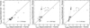 |
Fig. D.1. Comparison of lag estimates between ICCF and PyROA, ICCF and JAVELIN, and PyROA and JAVELIN, in the left, middle, and right panel, respectively. The black dashed line represents the 1:1 relation. The scatter around the 1:1 line is indicated in each panel. |
Appendix E: Lag analysis results for light curves from the literature
It is important to note that Edelson et al. (2024) performed a lag analysis of the Swift photometric light curves using the ICCF method, taking the W2 band as the reference. For consistency with our study, we reanalyzed the inter-band delays using the ICCF method with respect to the U band, which overlaps with the Strömgren u filter adopted as the reference band in our analysis. The obtained inter-band delays from Swift observations are given in Table E.1.
Results of Literature lag analysis.
All Tables
Results of lag analysis for the entire data (Total), for part 1 (S1), and for part 2 (S2).
All Figures
|
Fig. 1. Ultraviolet and optical spectra of Fairall 9 obtained with the HST Faint Object Spectrograph on 1993 January 21 and with the ESO 1.5 m telescope on 1994 July 14, respectively. Overplotted are the transmission curves of the OCM filters (u, v, b, y, and I) used for photometric observations in our HALO program, along with the transmission curves of Swift-UVOT filters (W2, M2, W1, U, B, and V) employed in constructing the photometric light curves in the literature. |
| In the text | |
|
Fig. 2. Light curves from OCM monitoring and lag analysis. Left: Light curves of Fairall 9 in the u, v, b, y, and I filters, shown from top to bottom, respectively. In each panel, the dashed lines in various colors indicate second-order polynomial detrending, while the solid lines represent the best-fit light curves obtained from PyROA. The full light curve is divided into two segments, S1 and S2, separated by an observational gap indicated by the vertical dashed orange line. Right: Distribution of the cross-correlation coefficient relative to the u band (solid black line) derived using the ICCF method for the full, non-detrended original light curve. The blue histogram shows the cross-correlation centroid distribution from ICCF, the red histogram represents the lag probability distribution obtained from PyROA, and the brown histogram shows the corresponding distribution from JAVELIN. A vertical dashed gray line marks the reference point at τ = 0 days. |
| In the text | |
|
Fig. 3. Results from the photometric flux variability analysis. Top: Optical SED of Fairall 9 derived from the mean fluxes in the u, v, b, y, and I filters. Middle: Differential SED constructed from the difference between the maximum and minimum fluxes in the corresponding filters. Bottom: Normalized excess variance, Fvar, as a function of wavelength. In both the top and middle panels, the dot-dashed teal line represents the best-fit power law with a free spectral index, while the dashed brown line corresponds to a power law with the index fixed at −4/3, as predicted by the standard thin accretion disk model. The orange-shaded regions indicate the ±1σ range, representing the wavelength uncertainty of each filter, as quantified by the rms width of its transmission curve. |
| In the text | |
|
Fig. 4. Spectral flux decomposition obtained with the FVG method. Black circles show the total flux density Fν. The host-subtracted AGN spectrum (blue circles) follows the thin accretion-disk prediction Fν ∝ ν1/3 (Shakura & Sunyaev 1973). The host component inferred from the FVG (red stars) is well matched by an Sb galaxy template (red curve; Kinney et al. 1996). |
| In the text | |
|
Fig. 5. Examples of lag-spectra based on ICCF lag measurements using the complete light curves for three cases: original (left), detrended with order = 1 (middle), and detrended with order = 2 (right). The ICCF lag measurements (red circles) are shown in the rest-frame as a function of rest-frame wavelength. The dot-dashed red line represents the best-fit to the relation τ ∝ λβ using Equation (5), where τ0, β, and α are free parameters. The dot-dashed black line shows the best-fit with fixed β = 4/3 and α = 1 with only τ0 as a free parameter. Shaded regions indicate the 1σ uncertainties from the fitting. The blue and maroon dashed lines show the respective best-fits derived without including τuI in the lag-spectrum for the cases where all parameters (τ0, β, and α) are free and where β = 4/3 and α = 1 are fixed. Vertical and horizontal dotted lines mark the rest-frame reference wavelength and zero rest-lag, respectively. |
| In the text | |
|
Fig. 6. Combined lag–spectrum. Red circular points show our HALO measurements, while black square points indicate reanalyzed literature measurements based on the light curve data from Edelson et al. (2024). The horizontal error bars represent the rms width of the transmission curve as the filter’s wavelength uncertainty. The dot-dashed red and black lines, together with their shaded regions, represent the best-fit results from power-law lag–spectrum fitting, with β and α treated as free parameters and fixed at 4/3 and 1, respectively. The corresponding fits obtained excluding τuI from the lag-spectrum are shown by the dashed blue and maroon lines. The lag–spectrum shows a clear excess in the u and U bands, suggesting Balmer continuum contamination from the BLR in these bands. |
| In the text | |
|
Fig. 7. Lag-spectrum modeling. Top: Ratio |
| In the text | |
|
Fig. A.1. Flux variation gradient diagrams for all filter pairs. Black points are the observed fluxes; the OLS-bisector fit (black line) gives the AGN slope ΓAGN (values in each panel). Dashed red lines show the range of host slopes from Sakata et al. (2010) (yellow region); their intersections with ΓAGN yield the host fluxes. Blue lines indicate the corresponding AGN flux ranges. |
| In the text | |
|
Fig. B.1. Comparison of the light curves of Fairall 9 in the Swift-U band (black points) from Edelson et al. (2024) (MJD 58251.6570−59259.1066) and the OCM-u band (blue-violet points) obtained during our HALO observing campaign (MJD 60573.2523−60719.0495), together with their respective detrending trends. The dotted and dashed lines show the detrending trends with order= 1 and 2, respectively. The Swift-U and OCM-u light curves exhibit distinctly different long-term detrending behaviors across their independent monitoring periods. This suggests that the detrending trend is strongly dependent on the overall duration of the light curve, as different time spans subtract different components of the slower variability from the observed signal. |
| In the text | |
|
Fig. D.1. Comparison of lag estimates between ICCF and PyROA, ICCF and JAVELIN, and PyROA and JAVELIN, in the left, middle, and right panel, respectively. The black dashed line represents the 1:1 relation. The scatter around the 1:1 line is indicated in each panel. |
| In the text | |
Current usage metrics show cumulative count of Article Views (full-text article views including HTML views, PDF and ePub downloads, according to the available data) and Abstracts Views on Vision4Press platform.
Data correspond to usage on the plateform after 2015. The current usage metrics is available 48-96 hours after online publication and is updated daily on week days.
Initial download of the metrics may take a while.