| Issue |
A&A
Volume 707, March 2026
|
|
|---|---|---|
| Article Number | A352 | |
| Number of page(s) | 14 | |
| Section | Extragalactic astronomy | |
| DOI | https://doi.org/10.1051/0004-6361/202556204 | |
| Published online | 17 March 2026 | |
Breaking through the cosmic fog: JWST/NIRSpec constraints on ionizing photon escape in reionization-era galaxies
1
Department of Astronomy, University of Geneva, Chemin Pegasi 51, 1290 Versoix, Switzerland
2
Cosmic Dawn Center (DAWN), Niels Bohr Institute, University of Copenhagen, Jagtvej 128, København N, DK-2200, Denmark
3
Niels Bohr Institute, University of Copenhagen, Jagtvej 128, Copenhagen, Denmark
4
Max Planck Institut für Astrophysik, Karl Schwarzschild Straße 1, D-85741 Garching, Germany
5
Department of Astronomy, The University of Texas at Austin, Austin, TX 78712, USA
6
Max-Planck-Institut für Astronomie, Königstuhl 17, D-69117 Heidelberg, Germany
7
Department of Astronomy & Astrophysics, University of Chicago, 5640 S Ellis Avenue, Chicago, IL 60637, USA
8
Department of Astronomy & Astrophysics, The Pennsylvania State University, University Park, PA 16802, USA
9
Institute for Computational & Data Sciences, The Pennsylvania State University, University Park, PA 16802, USA
10
Institute for Gravitation and the Cosmos, The Pennsylvania State University, University Park, PA 16802, USA
11
Department of Astronomy, University of Wisconsin-Madison, 475 N. Charter St., Madison, WI 53706, USA
12
Centro de Astrobiologí (CAB), CSIC-INTA, Ctra. de Ajalvir km4, Torrejón de Ardoz, E-28850 Madrid, Spain
13
LUX, Observatoire de Paris, Université PSL, Sorbonne Université, CNRS, 75014 Paris, France
★ Corresponding author: This email address is being protected from spambots. You need JavaScript enabled to view it.
Received:
1
July
2025
Accepted:
26
January
2026
Abstract
Aims. The escape fraction of Lyman continuum photons (fesc(LyC)) is the last key unknown in our understanding of cosmic reionization. Directly estimating the escape fraction (fesc) of ionizing photons in the epoch of reionization (EoR) is impossible, due to the opacity of the intergalactic medium (IGM). However, a high fesc leaves clear imprints in the spectrum of a galaxy, due to reduced nebular line and continuum emission, which also leads to bluer UV continuum slopes (βUV).
Methods. In this work, we exploited the large archive of deep James Webb Space Telescope (JWST) NIRSpec spectra from the DAWN JWST archive to analyze over 1400 galaxies at 5 < zspec < 10 and constrain their fesc based on spectral-energy-distribution fitting enhanced with a picket-fence model. We identify 71 high-confidence sources with significant fesc based on Bayes-factor analysis strongly favoring fesc > 0 over fesc= 0 solutions. We compare the characteristics of this high-escape subset against both the parent sample and established diagnostics including βUV slope, O32, and SFR surface density (ΣSFR).
Results. For the overall sample, we find that most sources have a low escape fraction (< 1%); however, a small subset of sources seems to emit a large number of their ionizing photons into the IGM, such that the average fesc is found to be ∼10%, as needed for galaxies to drive reionization.
Conclusions. Although uncertainties remain regarding recent burstiness and the intrinsic stellar ionizing-photon output at low metallicities, our results demonstrate the unique capability of JWST/NIRSpec to identify individual LyC leakers, measure average fesc, and thus constrain the drivers of cosmic reionization.
Key words: galaxies: high-redshift / early Universe / dark ages / reionization / first stars
© The Authors 2026
 Open Access article, published by EDP Sciences, under the terms of the Creative Commons Attribution License (https://creativecommons.org/licenses/by/4.0), which permits unrestricted use, distribution, and reproduction in any medium, provided the original work is properly cited.
This article is published in open access under the Subscribe to Open model. This email address is being protected from spambots. You need JavaScript enabled to view it. to support open access publication.
1. Introduction
The epoch of reionization (EoR) marks the last phase transition of the Universe, when the intergalactic medium (IGM) went from completely neutral to completely ionized (see, e.g., Becker et al. 2015; Dayal & Ferrara 2018; Robertson 2022; Fan et al. 2023 and Stark et al. 2026 for some recent reviews). This process starts with the formation of the first stars (Barkana & Loeb 2001) and does not conclude until z ∼ 5.3, as suggested by the scatter in opacity measured from the Lyman-α and Lyman-β absorption in quasar spectra (e.g., Eilers et al. 2018; Kulkarni et al. 2019; Yang et al. 2020; Bosman et al. 2022). Reionization is likely driven by star forming galaxies (e.g., Bouwens et al. 2015; Robertson et al. 2015; Naidu et al. 2020; Atek et al. 2024; Dayal et al. 2025) which can leak Lyman-continuum (LyC) photons (λrest < 912 Å) into the IGM. In this framework, the reionization process is very patchy (e.g., D’Aloisio et al. 2015; Bosman et al. 2018; Eilers et al. 2018; Yang et al. 2020; Bosman et al. 2022; Jamieson et al. 2025; Meyer et al. 2025), with bubbles forming around the objects that leak the most ionizing photons, which then expand and overlap until the entire Universe is ionized. Active Galactic Nuclei (AGNs) have also been suggested as possible contributors to reionization (Giallongo et al. 2015; Madau & Haardt 2015; Grazian et al. 2024; Madau et al. 2024), although other studies of the AGN luminosity function in the EoR have shown that their contribution is likely minor, compared to that of galaxies (Mitra et al. 2018; Hassan et al. 2018; Matsuoka et al. 2023).
To determine which sources are responsible for the bulk of reionization, we need to determine ṅion, which is the number of ionizing photons that reach the IGM per unit time and volume (Madau & Dickinson 2014; Robertson 2022). If we can rely on the UV light to trace the bulk of star formation in galaxies, this quantity, to the first order, can be expressed as
 (1)
(1)
where ρUV is the UV luminosity density (erg s−1 Hz−1 Mpc−3) calculated from the integral of the UV luminosity function, ξion is the ionizing-photon production efficiency (Hz erg−1), which measures the number of ionizing photons created per 1500 Å UV luminosity density, and fesc is the escape fraction of LyC photons; that is, the number of photons that escape the interstellar and circumgalactic media and reach the IGM.
Building on the results from the Hubble Space Telescope (HST), the James Webb Space Telescope (JWST) has allowed us to measure both ρUV (Bouwens et al. 2023; Donnan et al. 2024; Harikane et al. 2025; Whitler et al. 2025) and ξion (Simmonds et al. 2024a,b; Llerena et al. 2025; Pahl et al. 2025) during reionization. Therefore, one of the last major unknowns in our understanding of reionization is fesc, making this a key quantity.
Predictions from models (Bouwens et al. 2015; Robertson et al. 2013, 2015; Finkelstein et al. 2019; Naidu et al. 2020) indicate an average fesc∼5 − 20% over cosmic time for Equation (1) to work with globally averaged quantities, although this does not take into account obscured star formation (Simmonds et al. 2024c). Simulations that account for this source of ionizing photons predict lower fesc values, such as < 5% in SPHINX (Rosdahl et al. 2022) and ∼5%−10% at redshift 6 < z < 10 for THESAN (Yeh et al. 2023) and OBELISK (Trebitsch et al. 2021).
As important as fesc is, placing constraints on its value at z > 6 in the EoR is highly challenging due to the still partly neutral IGM. This is completely opaque to LyC photons and prevents the detection of LyC photons at z > 4.5, making direct observations of the escaped LyC flux and estimates of fesc in the EoR impossible (Inoue et al. 2014).
Until now, we had relied heavily on proxies and indirect indicators –calibrated at low redshifts where the LyC leakage can be directly measured– to estimate the fesc of EoR galaxies. Many studies have attempted to link various properties of known low-redshift LyC leakers to their fesc. The most comprehensive of these studies is the Low-Redshift Lyman Continuum Survey (LzLCS, Flury et al. 2022a,b), which observed 66 low-z (z = 0.2 − 0.4) galaxies, 12 of which are LyC emitters with fesc > 5%, and tested various indirect diagnostics. Other studies have tested the feasibility of the [Mg II] line (e.g., Chisholm et al. 2020; Xu et al. 2022), the C IV line (e.g., Saxena et al. 2022; Schaerer et al. 2022), the [O III]λ5007/[O II]λ3727 line ratio (O32; e.g., Jaskot & Oey 2013a; Nakajima & Ouchi 2014; Izotov et al. 2018b; Paalvast et al. 2018; Tang et al. 2021), the UV β slope (βUV; e.g., Chisholm et al. 2022; Flury et al. 2022b), star-formation-rate surface density (ΣSFR; Naidu et al. 2020), various properties of the Lyman-α line such as the double-peak separation (vsep; Verhamme et al. 2017; Izotov et al. 2018b; Naidu et al. 2022), or even multiple indicators together (e.g., Mascia et al. 2023, 2024; Jaskot et al. 2024a,b). However, many of these relations present large amounts of scatter, and, although they have been used to estimate fesc at high redshift (e.g., Navarro-Carrera et al. 2025), it is not obvious that relations calibrated on subsamples of galaxies at low redshifts (which often have unclear selection functions) will necessarily hold for the average galaxy in the EoR. Indeed, Pahl et al. (2024) found that this is not the case, at least when using the Lyman-α line shape as a proxy for LyC escape. They find different relations between fesc and the Lyman-α line shape at z ∼ 0.3 and z ∼ 3. Moreover, Witten et al. (2023) found that the fraction of neutral gas in the IGM has a strong impact on the red peak of Lyman-α, which would affect the shape of the line through cosmic time, and Giovinazzo et al. (2024) found the Lyman-α line alone is not sufficient to estimate LyC fesc in the EoR. Overall, a big caveat to the use of low-redshift analogs consists of the intrinsic differences between the low- and high-redshift Universe, due to differences in environment leading to fewer mergers and inflow of less pristine gas at later cosmic times, all of which can have an impact on the escape fraction. It is therefore evident that other methods for estimating fesc in the EoR are needed.
Thanks to the JWST and its NIRSpec instrument (Jakobsen et al. 2022), we now have deep rest-UV and rest-optical spectra of galaxies directly from the EoR. These provide access to all the information encoded therein, including information on fesc. Indeed, we expect the higher escape of ionizing photons to correlate with reduced nebular line and continuum emission, given the conservation of ionizing photons. Since nebular continuum emission and the presence of dust make the βUV slope redder, we can expect steep βUV slopes and weak nebular line emission (e.g., Hβ) to coincide with high fesc (Zackrisson et al. 2013, 2017; Chisholm et al. 2022; Marques-Chaves et al. 2022, 2024; Topping et al. 2022; Yanagisawa et al. 2025).
In this work, we exploited the large public archive of NIRSpec/PRISM spectra from a range of public JWST programs to analyze 1428 spectra of galaxies in the EoR and performed spectral-energy-distribution (SED) fitting with a picket-fence model on the spectra directly to estimate their fesc. For a similar work, see also Papovich et al. (2025).
In Section 2, we present the dataset that we used to perform this analysis. In Section 3, we present the picket-fence model, the SED fitting code we used, the selection of the high-confidence sample, and the line and size measurements. In Section 4, we describe how we validated our method with a recovery simulation. In Section 5, we present the main results, and we compare to other methods in Section 6. We discuss possible degeneracies and selection effects in Section 7, and, finally, we conclude in Section 8.
Throughout this work, we assumed flat ΛCDM cosmology with H0 = 70 km s−1 Mpc−1, Ωm = 0.3, and ΩΛ = 0.7. Magnitudes are given in the AB system (Oke & Gunn 1983).
2. Data
2.1. NIRSpec prism spectroscopy
The data in this work are part of the DAWN JWST archive (DJA1) (Heintz et al. 2025a; Brammer & Valentino 2025), an online repository containing spectroscopic data from public JWST programs, all uniformly extracted and reduced with the same pipeline, which makes use of grizli2 and MSAexp3. Further details on the data reduction and processing can be found in de Graaff et al. (2025), Heintz et al. (2025a), Valentino et al. (2025) and Pollock et al. (2026). We performed our database query on 7 February, 2025 and include all sources with available PRISM/CLEAR spectra at 5 < z < 10 with grade = 3 (i.e., with a robust redshift measurement based on visual inspections) and available photometry in at least one JWST NIRCam filter (as described in Section 2.2), which is needed to estimate sizes and slit-loss corrections.
The spectra stem from various public surveys, including RUBIES (GO 4233, de Graaff et al. 2025), JADES (GTO-1180, 1181, 1210, 1286, 1287; GO-3215 Eisenstein et al. 2026), GO-3215 (Eisenstein et al. 2025), GTO WIDE (GTO-1211, 1212, 1213, 1214, 1215; Maseda et al. 2024), CEERS (ERS-1345; Finkelstein et al. 2023), UNCOVER (GO-2561, Bezanson et al. 2024), CAPERS (GO-6368; PI: Dickinson), GO-1433 (Hsiao et al. 2024), GO-2198 (Barrufet et al. 2025), GO-2565 (Nanayakkara et al. 2025), DD 2750 (Arrabal Haro et al. 2023), GO-3073 (Castellano et al. 2024), DD-2756 (PI: Chen), DD-6541 (PI: Egami), DD-6585 (PI: Coulter), and GO-4106 (PI: Nelson). The number of sources corresponding to each program can be found in Table 1. The redshift constraints that we applied to our sample allowed us to select sources in the EoR that also have coverage of the Hβ line, which is bright enough to be detected in most galaxies and is also visible at high redshifts. We applied a UV-magnitude cut at MUV = −18. The distribution of MUV as a function of redshift is shown in Figure 1, which only shows a slight evolution toward brighter MUVs with increasing redshift. Lastly, we removed 64 broad-line LRDs reported in Kocevski et al. (2025). We did not remove any other AGNs as they are unlikely to have a significant impact on the identification of leakers in our framework where we expect high fesc sources to have very faint lines. In total, our sample consists of 1428 galaxies at 5 < zspec < 10. While this wide selection gives us access to a large amount of data, it also leads to an effectively unknown selection function with varying exposure times. The possible impact of this is addressed in Section 7.
Overview of sources included in our analysis.
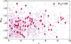 |
Fig. 1. Distribution of MUV as function of redshift for the whole sample. The high confidence sample (see Section 3.3) is highlighted with diamond markers, while the parent sample of spectroscopic redshifts is shown as dots. |
2.2. Photometry
Based on the JWST and ancillary HST imaging available on the DJA, we derived photometric catalogs following Weibel et al. (2024). We used an inverse-variance weighted stack of the long wavelength filters F277W, F356W, and F444W as the detection image, and measure fluxes in circular apertures of 0.16″ radius in point spread function (PSF) matched images. These aperture fluxes were first scaled to the flux measured through Kron ellipses in the detection image. Additionally, we placed each Kron ellipse on the F444W PSF and divided by the encircled energy to account for flux in the wings of the PSF.
The photometric data were needed to correct flux-sensitive quantities such as UV magnitudes and masses, as in many cases the slit is positioned such that only a part of the galaxy is observed. Using the photometry helped us estimate slit-loss corrections. We performed these corrections by creating synthetic photometry from the spectra and scaling this synthetic photometry to the real photometry using a wavelength-independent scaling. The typical rescaling factors hover around 1, with a median of 1.1 and a standard deviation of 0.6, indicating that the msaexp corrections are accurate and that most of our sources are compact, as expected at high redshift. We used this uniform scaling to correct the UV magnitudes and the masses estimated from the spectra. We also used the photometry to fit for galaxy sizes. The fitting process is described in detail in Section 3.4.
3. Methods
3.1. Picket-fence model
To estimate fesc with bagpipes, we implemented a picket-fence (Heckman et al. 2001; Zackrisson et al. 2013) model. With this model, we assume that stars are partially covered by an optically thick ISM, with some channels of low column density (and no dust) that allow for ionizing photons to escape. Effectively, this means that only a fraction of a source is covered by optically thick gas, so fesc is estimated as fesc = 1 − Cf, where Cf is the covering fraction. In the SED fitting, this means that the output spectra will be a linear combination of fesc = 0 models in the fraction that is covered by gas and fesc = 1 and AV = 0 models in the free channels. While this model has been found to not exactly reproduce the fesc from radiative transfer in simulations, it is in reasonable agreement (Mauerhofer et al. 2021) and has been used before at redshift 3 < z < 5 to connect UV absorption features to fesc (Saldana-Lopez et al. 2023).
The effects of the picket-fence model on a spectrum are shown in Figure 2. Note that we would expect similar traces of fesc on the spectra from a density-bounded model, at least in a dust-free scenario (Zackrisson et al. 2013). The galaxy modeled in Figure 2 is at redshift of z = 6 and has a stellar mass of M* = 109 M⊙, a metallicity of Z = 0.05 Z⊙, an ionization parameter of log U = −2, a dust attenuation of AV = 0.2 modeled with a Calzetti (Calzetti et al. 2000) dust model, and a constant star formation history (SFH) that is switched on at 5 Myr. The only parameter that we modified between the various models is fesc, which we did to highlight the effect of this quantity on a mock galaxy. As fesc increases, there is a clear steepening of the βUV slope and weakening of all the emission lines, as highlighted in the bottom panels: one for Hα (left) and one for Hβ+[O III] (right). There is also an effect on the continuum in the optical part of the spectrum, which is reduced due to an overall reduction or absence of the nebular continuum contribution.
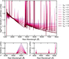 |
Fig. 2. Top: spectrum of a model galaxy with various fesc. The model galaxy is at z = 6 and has a mass of M* = 109 M⊙, metallicity of Z = 0.05 Z⊙, ionization parameter of log U = −2, constant star formation switched on at 5 Myr, and dust modelled via the Calzetti (Calzetti et al. 2000) dust curve with Av = 0.2. As fesc increases, the βUV slope becomes steeper due to reduced nebular continuum emission, and the emission lines become weaker. The continuum emission is also affected as its nebular component scales with fesc. The full spectrum thus contains information on the escape fractions, which we exploited to constrain the fesc of galaxies with NIRSpec spectra. Bottom left: zoomed-in view of Hα. Bottom right: zoomed-in view of Hβ+[O III]. |
It is possible for the βUV slope to redden due to dust or an older stellar population; however, here we simply highlight the effects of fesc on the spectrum. These effects should make it possible to estimate it at any redshift, as long as the βUV slope and emission lines are covered in the spectrum, which they are in the EoR when observing with the PRISM configuration of NIRSpec.
3.2. SED fitting
We implemented a picket-fence model in the bagpipes SED fitting code4 (Carnall et al. 2018, 2019; Lange 2023). This was then applied directly to the spectra to estimate the physical properties of our sources, including fesc. Our custom version of bagpipes also employs updated CLOUDY grids (Ferland et al. 2017) that were run without internal dust (i.e., with grains ISM turned off). This solves an issue with the emission-line normalizations in the original bagpipes grids.
The choices of free parameters, their ranges, and priors are outlined in Table 2. The range for logU is based on the results of Reddy et al. (2023). We also fit for the redshift using a very narrow Gaussian prior, with a standard deviation of only 0.002, centered at the spectroscopic redshift zspec. We used the BPASS v2.2.1 stellar-population models (Stanway & Eldridge 2018) with the default broken-power-law initial mass function (IMF), with slopes of α1 = −1.30 for the 0.1 − 0.5 M⊙ mass range and α2 = −2.35 for the 0.5 − 300 M⊙ mass range, based on Kroupa et al. (1993). To estimate the stellar and nebular attenuation, we used the Calzetti dust law (Calzetti et al. 2000), allowing for a maximum AV = 0.5 as we were mainly interested in blue sources. This choice did lead to poor fits for very dusty galaxies, which are unlikely to be leakers and therefore will only be in the background sample. We modeled the SFH with the continuity prior (Leja et al. 2019) in bagpipes, a nonparametric model, which allows for greater flexibility in the SFHs than parametric models would. Using this prior, we estimated the star formation rate (SFR) in seven bins – with 5, 10, 50, 100, 200, 400 and 800 Myr – unless the age of the Universe at the source’s redshift was less than 800 Myr. In that case, the last bin ended at the age of the Universe. With the continuity prior, bagpipes fits for the ΔSFR between adjacent bins, which therefore adds a number of free parameters equal to the number of bins minus one. We used a Student-t prior with ΔSFR ∈ [ − 3, 3] and adopted ν = 2 and σ = 0.3 following Leja et al. (2019). We opted for a logarithmic prior for fesc as observations seem to suggest that most sources have little to no leakage (Kreilgaard et al. 2024), which is more consistent with a logarithmic than a constant distribution. When performing the fit, we chose to mask the spectrum below rest-frame wavelengths of λr < 1300 Å to avoid fitting the Lyman-α line or the IGM attenuation, which can vary from source to source and may include damped Lyman-α (DLA) absorption profiles (Heintz et al. 2024, 2025b; Mason et al. 2026; Meyer et al. 2025).
Bagpipes parameters used for SED fitting.
3.3. High-confidence sample selection
To identify which galaxies are more likely to be leakers, we performed a second run with a fixed fesc = 0 throughout our sample. We then compared the statistical evidence of the two different runs by calculating the Bayes factor over the unmasked (λr > 1300 Å) region. This helped us determine how likely a high fesc solution is compared to a low fesc solution and select galaxies for the high-confidence sample. The Bayes factor, introduced by Jeffreys (1939), compares the evidence of two models with equal priors and quantifies the pertinence one model over the other, given the data. It is defined as
 (2)
(2)
where M1 and M2 are the models being tested and y represents the data the models are being tested on. In our case, the models being tested are one with variable fesc and the fesc = 0 model, given the priors and model used. Therefore, a high Bayes factor implies that fesc > 0 is favored with respect to the fesc = 0 solution. We computed the Bayes factors for the full spectra and used them to determine a high-confidence sample. To do this, we followed the table provided by Kass & Raftery (1995) and chose to consider Bayes factors greater than 100 as decisive evidence. We therefore selected the high-confidence sample to include galaxies with a Bayes factor of B12 > 100. With these criteria, we initially identified 74 high-confidence LyC leakers. We visually inspected all sources and removed three objects with poor fits. After the visual inspection, we were then left with 71 sources that we considered the high-confidence sample of LyC leakers. This sample is identified in all our scatter plots via the diamond markers.
The spectrum of one of our high-fesc candidates, together with the two fits, is shown in the first panel of Figure 3. For this source, the Bayes factor was calculated to be 1.06 × 10⁴, which indicates that the high-fesc solution is a much better fit for the data. The most striking difference between the two models is in the βUV slope, which the high fesc model can fit well. The fesc = 0 model cannot reproduce such a blue slope, resulting in a mismatch with the data. This is highlighted in the middle panel, where we show the difference between the two models.
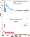 |
Fig. 3. Example galaxy with Bayes factor > 100. Top: observed spectrum (blue line) and the two models, one with high fesc (solid orange line) and one with fesc = 0 (dashed magenta line). The shaded gray region represents the masked area. A clear difference between the two models can be seen in the βUV part of the spectrum, where the high fesc solution fits the data much better than the other solution. Middle: difference between two models highlighting the difference in the βUV slope and to some extent in the emission-line strengths. Bottom: Comparison of SFH for the two models. The models are extremely different, as reproducing the weak lines and steep βUV slope without fesc is only possible with a recent quenching of star formation. This indicates a degeneracy between SFH and fesc, which is discussed further in Section 7. |
In the same figure, we also show the SFH of the two models. The difference stems from the different mechanisms required by bagpipes to match the spectrum: high fesc in one case and post starburst in the other. There is therefore some level of degeneracy between the estimation of fesc and that of the SFH. This is discussed in more detail in Section 7.
3.4. Size measurements
One potential tracer of fesc proposed by Sharma et al. (2016, 2017) and Naidu et al. (2020) is the SFR surface density. Hence, we also estimated the effective radii (reff) of our sources. For this, we used imaging data from JWST/NIRCam in the F115W, F150W, or F200W filters, depending on the redshift of the objects. As we were interested in the size in the UV, we selected the filter that contains 1600 Å in the rest-frame wavelength; if this wavelength was not covered by any filter, we used F115W as it is the bluest filter. Hence, we used F115W in the 5 < z < 7.3 range, F150W in the 7.3 < z < 9.3 range, and F200W for z > 9.3. The short wavelength filters are not always available, so for some sources (107) it was impossible to calculate the sizes in the UV.
The fitting was performed with pysersic (Pasha & Miller 2023) using the variational inference method svi-flow. We used uniform priors for reff and n with ranges of [0.25, 10] kpc and [0.65, 6], respectively. For the center pixels, we used Gaussian priors with the mean as the center of the cutout and a one-pixel standard deviation. We masked all neighboring sources and used the empirical PSF models described in Weibel et al. (2024). All other priors were set with the autoprior function of pysersic.
3.5. βUV slope and line measurements
The UV continuum of galaxies can be characterised by a power law:
 (3)
(3)
where β is the UV-slope, βUV. We measured the UV slope from the best-fit SED in the 1268 < λ < 2580 Å range. We chose to exclude ten windows, as described by Calzetti et al. (1994), in order to avoid stellar and interstellar absorption features affecting the shape of the continuum. This ensured that we fit the continuum and that our fit was not contaminated by the lines. We chose to measure the βUV slope from the SED, as bagpipes simultaneously fits to the βUV slope and the lines, therefore allowing us to make use of all the information in the spectrum. In this context, the error on the βUV slope was derived by calculating the βUV slope of all the spectra of the bagpipes posterior and by taking the 16th and 84th percentiles of the βUV distribution.
For consistency, we also measured the equivalent width of Hβ from the best fit SED using the indices function within bagpipes. We took the line fluxes for [O III] and [O II] from the DJA;5 they were extracted using masexp.
4. Validation
Before applying our method to all of the spectra, we performed some validation tests. Since we used data from very different programs, with different selections, it is necessary to understand how our method behaves at different signal-to-noise ratio (S/N) levels. We thus performed a recovery simulation to determine how well bagpipes can recover a known escape fraction from a model spectrum when noise is added. We performed this test on a model galaxy from bagpipes, with every model parameter fixed except for the escape fraction, which we varied using nine values. We then normalized the spectra to obtain results consistent with the SED fits on the NIRSpec spectra. To do this, we calculated the median continuum flux at 5100 Å < λr< 6500 Å for the overall sample and scaled each model spectra with a factor of fnorm = ⟨fν,NIRSpec⟩/⟨fν,model⟩, where the median continuum flux for the model spectrum was calculated in the same wavelength range. We would like to note that the uncertainties that noise added to our estimation of fesc may have been larger if different input SEDs had been tested. As all parameters except for fesc were fixed, we can confirm that we provide lower limits to the fesc.
We then ran the normalized model with the given escape fraction through the JWST exposure time calculator (ETC)6 to degrade the bagpipes SED model to prism resolution. This also gave us the S/N curve, which we used to add the desired level of noise.
We used four different S/N levels –3, 5, 10, and 20– calculated between rest-frame wavelengths of 1300 Å < λr < 1800 Å. For each fesc and S/N value, we created three different instances of Gaussian noise that is added to the input spectra, thus giving us three realizations of spectra per fesc and S/N value. Each of the spectra is fit with bagpipes using the same setup as the one used for the real NIRSpec spectra. We also performed a fesc = 0 run to determine the Bayes factor.
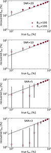 |
Fig. 4. Results of recovery simulation. The open markers indicate a Bayes factor of < 100, while the filled markers indicate a Bayes factor of > 100. The dashed black line indicates the 1:1 line, i.e., the true values. Our method can recover the high-fesc galaxies with a high confidence at all signal-to-noise levels, while we can also recover lower fesc values at high S/N levels. |
The results of the recovery simulation are shown in Figure 4, where each panel features a different S/N level. In all the panels, the filled points indicate that the Bayes factor is > 100, while the empty points have a Bayes factor of < 100, and the dashed line indicates the 1:1 line (i.e., the truth line). At S/N = 20, all the runs except for fesc = 10% have a high Bayes factor, and while the high-fesc points are on the truth line, the low fesc (< 50%) are slightly overestimated. In the S/N ≤10 cases, the Bayes factors for the lowest fesc values become < 100, and the uncertainties increase. Overall, the results are consistent with the truth, except when S/N = 3, for all fesc < 30%, and where all the recovered fesc are consistent with fesc = 0. We can thus conclude that our method is robust and can safely recognize high-fesc sources even at low signal-to-noise levels.
5. Results
Having validated our picket-fence model fitting on NIRSpec data, we now present our results from the SED fitting to the sample described in Section 2.1. We present the inferred fesc and other properties of the sources.
5.1. βUV versus EW0(Hβ)
We start by showing the relation between βUV slopes, the rest-frame equivalent width (EW0) of Hβ – both calculated from the best-fit SED – and fesc in Figure 5. The βUV - EW0(Hβ) plane was already proposed by Zackrisson et al. (2013) to identify high-fesc sources, predicting high fesc to correlate with steep βUV slopes and EW0(Hβ) < 150 Å. However, this is not seen in the LzLCS sample (Flury et al. 2022b). We indeed find a correlation between steep βUV slopes and high fesc: below βUV = −2.5 we find no low fesc galaxies. This correlation stems from the fact that the addition of nebular continuum reddens the slope. For a young stellar population, this reddening pushes the βUV slope from ∼−3.0 up to ∼−2.5, almost independently of the chosen IMF (Katz et al. 2025; Yanagisawa et al. 2025). In the case of BPASS, it is only possible to have βUV < −2.5 if the nebular continuum is reduced, due to a nonzero fesc. We do not see a relation with EW0(Hβ). Many high-fesc galaxies have an EW < 200 Å, but no clear trends with decreasing EW are visible. In the same figure, we also highlight our high-confidence sample of 71 galaxies with a Bayes factor of > 100 via the diamond markers. As expected, all of these sources have very blue βUV slopes, mostly below −2.5, making the fesc = 0 solution unlikely.
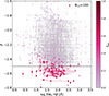 |
Fig. 5. βUV slope versus EW0 of Hβ, color-coded by fesc. The parent sample is shown as circles, and the high-confidence sample is highlighted with diamond markers. All of the high-confidence sources occur at a low βUV slope, with most having a βUV slope of < − 2.5, but they span the entire EW range. |
5.2. fesc versus βUV
In Figure 6, we analyze the fesc distribution as a function of the βUV slope and the evolution of mean fesc with bins of the βUV slope. The mean fesc was calculated over the whole parent sample, and the uncertainties on the mean were computed by resampling each fesc value over its posterior 1000 times to properly account for measurement uncertainties. We find a consistent decrease of mean fesc as slopes get shallower, indicating an overall redder spectrum, as expected from our model. This trend is qualitatively consistent with the results of both Chisholm et al. (2022) and Jaskot et al. (2024a) shown in the same plot, although our relation is steeper. Both relations from the literature are based on a sample of 89 z = 0.3 galaxies, with the main difference between their methods being the use of survival analysis in the case of Jaskot et al. (2024a), using the LyCsurv code (Flury et al. 2024). This indicates that, on average, galaxies that leak a lot of their ionizing continuum are those that have a steep βUV slope.
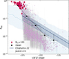 |
Fig. 6. fesc versus βUV slope. The darker diamond points highlight the high-confidence sample, while the dots represent the parent sample. The squares represent the average fesc in βUV bins, calculated from the parent sample. The fesc − βUV relation from Chisholm et al. (2022) is shown as the dashed line, with the uncertainty shown as the shaded area. With the dotted line, we show the results of Jaskot et al. (2024a), using the LyCsurv code (Flury et al. 2024). The average fesc decreases as the βUV slope becomes bluer. |
We again see the limit of βUV ∼ −2.5, as calculated from the best-fit model, below which it is very difficult to have fesc = 0; this is due to the impact of the nebular continuum on the slope. Although the overall shape of the relation is similar, it must be noted that the βUV < −2.5 range is almost unpopulated in the LzLCS sample, possibly due to more dust being present at low redshift.
We also see a large amount of scatter in the relation, which is not symmetric, toward lower values of fesc. We find a larger scatter in the relation than that found by Chisholm et al. (2022). Overall, the trend that we find seems to be mostly driven by the necessarily higher fesc at low (βUV < −2.5) βUV values rather than by a real, smooth decrease in fesc with a reddened βUV. The mean fesc values indeed decrease exponentially to a redder βUV. Around βUV ∼ −2.5, we see a steep drop in many fesc values, which is likely due to the fact that the spectra of these sources do not contain significant information on the fesc values, such that they end up spanning almost the full range of the prior distribution. This also leads to a particularly large dispersion in fesc values around βUV of −2.5 to −2.2.
5.3. fesc versus MUV
To fully understand reionization, it is important to identify which subpopulation of galaxies leaks the most ionizing photons: faint or bright ones. For this reason, we show the relation between fesc and MUV in Figure 7.
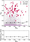 |
Fig. 7. Top: fesc versus MUV. The parent sample is shown with the pink dots, the high-confidence sample is shown by the dark diamonds, and the average fesc in bins of MUV is shown as the black squares. The mean fesc does not show a trend with MUV. The average fesc of our sample is consistently measured between 10 and 15% in all bins. Bottom: fraction of sources with fesc > 0.1 in each UV magnitude bin. This fraction also shows no trend with MUV. |
Both the high-confidence sample and the average fesc do not show a clear trend with MUV. At all magnitudes, the average fesc sits at around 10%, which is consistent with the results of Mascia et al. (2025), but in contrast with the results of Papovich et al. (2025), which found a much lower average fesc: ⟨fesc⟩∼3%.
In the bottom panel of the same figure, we present the fraction of objects with fesc > 0.1 in each MUV bin. This also remains mostly flat with MUV.
This implies that the trends in mean fesc are due to the amount of leaker galaxies compared to non-leakers. Tabulated values of both the average fesc and the fraction of galaxies with fesc > 0.1 in each magnitude bin can be found in Table 3 to facilitate reading.
Tabulated means and standard deviations of ⟨fesc⟩.
Our values are consistent with current models of reionization, which suggest that mean fesc values of about 5%–20% are needed to reionize the Universe by z ∼ 6 (Bouwens et al. 2015; Robertson et al. 2015; Finkelstein et al. 2019). Our results would thus imply that bright and faint galaxies have an equal number of strong leakers and that both bright and faint galaxies contribute. A more detailed discussion will be presented in Giovinazzo et al. (in prep.) We note, however, that it is possible that our sample is lacking some high-fesc sources at faint magnitudes, as faint sources with no lines might not have high-confidence redshifts in the DJA or might not have been targeted. It is therefore possible that our inferred average fesc at faint magnitudes could be somewhat underestimated.
5.4. The cumulative distribution function of fesc
A good test to determine if our fesc distribution is consistent with reionization models is to compare the cumulative distribution function (CDF) of our inferred fesc values with simulations that also estimate fesc. We compared our CDF to the CDF of three simulations: (1) SPHINX (Rosdahl et al. 2022; Katz et al. 2023), which we calculated from the entire SPDRv1; (2) OBELISK (Trebitsch et al. 2021), which we calculated from all the main snapshots at 5 < z < 9.6; and (3) the three models of SPICE (Bhagwat et al. 2024). For both SPHINX and OBLEISK, we applied the same MUV < −18 cut as we did for the parent sample. Although we applied the same cuts to the simulations as we did to the observations, it is important to note that the selection function of the observed sample is not well characterized, making the comparison between observations and simulations not obvious. Our results are shown in Figure 8.
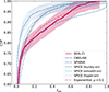 |
Fig. 8. Empirical cumulative distribution function (CDF) of fesc in the parent sample. The solid dark pink line shows the CDF for our data, with the shaded area representing the 95% confidence interval. The dotted lines with the shaded areas show the CDF of different simulations, including SPHINX and OBELISK, with the respective 95% confidence interval. The dashed blue lines show the three realizations of the SPICE simulation. The dot-dashed purple line represents a simple exponential distribution with a mean of 10%, as justified by the results of Figure 7, and which fits our CDF rather well. All models consistently predict mostly low-fesc objects, with a few high-fesc sources that drive the mean fesc to non-negligible values. |
We also show the CDF of an exponential distribution of fesc, similar to that presented in Kreilgaard et al. (2024) but with a mean fesc of 10%, which is more in line with our measurements, as shown in Figure 7. Our CDF shows that most of the sample has extremely low fesc and few galaxies have very high fesc, with only about 20% of the sample showing fesc > 0.2. This is broadly consistent with all of the simulations, the CDFs of which all show a large number of very low fesc galaxies, but differ in amounts of high-fesc sources. Both OBELISK and SPHINX contain a much larger fraction of sources with very low fesc with respect to our sample, which could be due to ionizing photons produced by obscured star formation; these were not taken into account in our model, but they were in the simulations. Taking this source of ionizing photons into account can lower the inferred escape fraction, possibly leading to the discrepancy between OBELISK and SPHINX and our model.
The simulation that is most consistent with our results is the bursty-sn model of SPICE. Out of all the SPICE models, this is the only one that reionizes at a time consistent with observations (Bhagwat et al. 2024), which is very encouraging for our results. The exponential model is also entirely within our confidence interval, showing good agreement with our data. This indicates that our method results in a consistent fraction of high-fesc galaxies that is compatible with current models of reionization, even if we cannot determine the completeness of our sample well.
5.5. High-confidence versus parent sample
Next, we wanted to test if the high-confidence, high-fesc sample has any particular properties that set it apart from the parent population at the same redshift. To do this, we compared the physical properties derived from bagpipes between our high-confidence sample and the parent sample. We present this comparison in Figure 9. Looking at the specific star formation rate (sSFR = SFR10/M*) distributions, it is clear that, on average, the high-confidence sample has a higher sSFR than the parent sample, which is in line with the model of Ferrara et al. (2025). Our candidate leakers are thus likely to have gone through a recent burst of star formation, consistent with results from simulations (e.g., Trebitsch et al. 2017). This is also seen in the age distributions, which indicate that all the high-confidence fesc sources have ages < 0.2 Gyr, while the parent sample has sources with ages up to 0.6 Gyr.
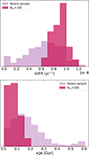 |
Fig. 9. Top: comparison of specific SFR distribution between the parent sample (light pink) and the high-confidence sample (dark pink). Bottom: comparison of age distribution between the parent sample and the high-confidence sample. The high-confidence sample is both more star forming and younger, indicating a relation between these properties and LyC leakage. |
From this figure, we can say that, overall, our sample of confident leakers is more star forming and younger than the parent sample. This is consistent with the conditions for production and escape of ionizing photons, as young stars are those that can produce LyC photons and are also required to produce very steep UV slopes (βUV < −2.5).
6. Comparison with other methods to indirectly estimate fesc
There have been many attempts in the literature at linking fesc to other characteristics of galaxies, such as the [O III]λ5007/[O II]λ3727 line ratio (O32; e.g., Jaskot & Oey 2013a; Nakajima & Ouchi 2014; Izotov et al. 2018b; Paalvast et al. 2018; Tang et al. 2021), the βUV slope (e.g., Chisholm et al. 2022; Flury et al. 2022b), star formation rate surface density (ΣSFR; Naidu et al. 2020), and those discussed in Section 1. In this section, we explore some of these methods and determine if our data follow the relations previously found in the literature.
6.1. The O32 line ratio
We first explored O32 (defined as [O III]λ5007/[O II]λ3727), an indicator for fesc that has been studied both from simulations and observations, but for which a clear understanding of its suitability to estimate fesc is still lacking. High O32 ratios might be indicative of density-bounded conditions, and therefore high fesc, but its dependence on ionization parameter and metallicity (Sawant et al. 2021) makes its interpretation challenging. Simple photoionization models show a correlation between O32 and low optical depth for LyC photons (Jaskot & Oey 2013b; Nakajima & Ouchi 2014), while results from simulations show no clear trends between fesc and O32 (Katz et al. 2020; Barrow et al. 2020; Choustikov et al. 2024). Low-redshift observations also show a tenuous relation with varying degrees of scatter in the fesc–O32 plane (Faisst 2016; Nakajima et al. 2020; Flury et al. 2022b), showing that while many LyC leakers present a high O32, this condition alone is not enough to identify leakers. This is also seen in our sample in Figure 10. Many sources with high O32 ratios do indeed show fesc > 0.2, but the average values in bins of O32 only increase very slowly. This result is consistent with those of Choustikov et al. (2024), which also found no clear trend between fesc and O32 in the SPHINX simulation.
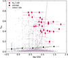 |
Fig. 10. Relation between fesc and O32, with the average fesc shown as black squares, in bins on log(O32). The diamond points represent the high-confidence sample, and the dots show the parent sample. The dashed gray line shows the relation between fesc and O32 form Izotov et al. (2018a). The gray triangles indicate lower limits on the O32 ratio for the points with S/N([O II]) < 3. Our points show no strong trend between ⟨fesc⟩ and O32. |
It is important to note here that the relation between O32 and fesc was proposed for a density bounded scenario, whereas we assumed a picket-fence model in our SED fitting, which could be the cause of the discrepancy with the low-redshift observations. However, the agreement with the result of SPHINX by Choustikov et al. (2024) could imply that this relation might not be easily applicable at high redshift.
6.2. A high SFR surface density
We also looked at the star formation rate surface density, defined as
 (4)
(4)
where we used SFR10 for the star formation rate. LyC leakers have previously been found to be generally compact with high ΣSFR (Sharma et al. 2016, 2017; Naidu et al. 2020; Flury et al. 2022b). Others found that UV compact sources are more likely to be LyC leakers (Marchi et al. 2018). This suggests that highly concentrated star-forming regions might create the ideal conditions for feedback to clear paths in the ISM to leak ionizing radiation (Flury et al. 2022b). In Figure 11, we show fesc versus ΣSFR for our sample.
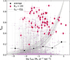 |
Fig. 11. fesc versus star formation rate surface density. The high-confidence sample is shown with the dark diamonds, and the average fesc is shown with the black squares. Our sample does not show any significant trend of higher fesc with higher ΣSFR, as was expected from the proposed relation from Naidu et al. (2020) that is shown as the dashed line. |
We compared this to the proposed relation from Naidu et al. (2020), fesc ∝ (ΣSFR)0.4. Our sample clearly does not follow this simple scaling. Although there may be a mild trend toward higher escape fractions, this is not significant at higher ΣSFR on average. There is again enormous scatter in the individual measurements, and it is certainly not the case that all sources with very high ΣSFR have high escape fractions. In summary, we conclude that none of the previously proposed “simple” relations to estimate fesc are consistent with our results, apart from the strong trend with UV continuum slope.
7. Discussion
7.1. Selection
Our choice to use all the NIRSpec/prism spectra from the entire DJA gives us access to an unprecedented amount of deep rest-optical spectra in the 5 < z < 10 redshift range, but it also comes with important considerations about the selection. First of all, the choice of only using sources with grade = 3, although necessary to ensure that the objects are fit at the correct redshift, biases the sample toward line emitters. As the grades are assigned through visual inspection, sources with stronger Lyman breaks and stronger lines are more likely to receive a high grade. Because of this, we are possibly missing leakers with very weak lines, especially at the faint end of our magnitude range. We note that this selection can also lead to a bias toward intrinsically brighter sources at higher redshifts, as fainter sources may not receive a high grade through visual inspection.
Second, the choice of using a wide array of different programs makes the selection function essentially intractable. Many of the spectra used here were only included as filler targets in individual masks. It is therefore difficult to know if our results are valid for a UV- or mass-selected sample of galaxies, as it is unclear what kind of biases enter our sample through the mask design strategies of the different programs. This will have to be tested with future initiatives that aim to obtain mass-selected galaxy samples with prism spectroscopy.
7.2. Method caveats
Until now, we have focused on the role of the βUV slope and the Balmer lines as indicators of high fesc that can be used in the EoR. However, there is another possible scenario that could lead to a source having a steep βUV but weak Balmer lines, which is the case of a recently quenched source that has had star formation within the last 100 Myr (Looser et al. 2024). In such cases, O-type stars with lifetimes of ≲10 Myr have already died (reducing the observed nebular emission), while less massive B-type stars (with lifetimes of ∼100 Myr) would still be present, producing slightly steeper UV slopes. This indicates a possible degeneracy of our results with the SFH, as most of our high-confidence sources have a very blue βUV slope but weak Hβ. This is exemplified in the third panel in Figure 3, where we compare the SFH of a single galaxy for the high-fesc case to the no-fesc case. However, the same example also shows that even with a recent quenching SFH, the fesc = 0 cannot match the data quite as well, as quantified by the very high Bayes factor. It is important to note that we fit everything together –fesc and SFH– and therefore this degeneracy was included in the uncertainties of fesc, which were computed as the 16th and 84th percentiles of the posterior distribution and are small for our high-confidence sample. We also note that none of these high-confidence sources show any signs of a Balmer break, which one could expect to appear if the star formation was suppressed for long enough. We would like to comment on the fact that our quantitative results should only be interpreted within the modeling framework we used here, i.e., using the BPASS v2.2.1 stellar population-synthesis models and the specific dust-extinction prescriptions. While systematic uncertainties arising from alternative stellar evolution models, stellar spectral libraries, or dust-extinction laws could impact our quantitative conclusions, we do not expect the results to change qualitatively. Nevertheless, it is important to fit sources with known, directly measured escape fractions and with NIRSpec/prism spectra to further test our method in the future.
8. Summary
In this paper, we present the addition of a picket-fence model to bagpipes as a new tool to recover fesc from the spectra of EoR galaxies. This allows the direct estimation of this important parameter for reionization, without the need for indirect tracers calibrated at lower redshift.
Using public NIRSpec/prism spectra and photometry available in the DJA, we compiled 1’428 galaxies at redshifts 5 < zspec < 10 from a variety of public programs (see Table 1). We derived the physical properties and fesc of each source through SED fitting on the spectra, using the picket-fence model with bagpipes. We performed a second bagpipes run with fesc = 0 and quantified the best-fit model with the use of the Bayes factor. In doing this, we identified 71 galaxies as high-confidence LyC emitters based on their Bayes factor (B12 > 100).
We validated our picket-fence model by performing a recovery simulation with various noise levels and find that the SED fitting can recover the correct fesc, with the exception of low-fesc values at low S/N, which are underestimated. High-fesc values were always recovered correctly and with high confidence (B12 > 100).
The main results from our analysis are listed below:
-
The high-confidence LyC leaker sample is mostly characterized by blue βUV slopes, < − 2.5. The average fesc of the overall sample decreases with increasing βUV slope, making it broadly consistent with results from Chisholm et al. (2022) and Jaskot et al. (2024a). This shows that the βUV is also an important indicator for fesc at high redshift when applied as a general trend.
-
There is no significant trend of fesc as a function of MUV. Overall, we find average fesc values at all magnitudes hovering around 10-15%. This is consistent with the required values for completing reionization with galaxies alone by z ∼ 6, as discussed in the past literature.
-
The cumulative distribution function of the fesc measured with our method is consistent with simulations. We find that most of our sources have very low fesc, with only a few high-fesc sources, as expected. The closest model to our CDF is the bursty-sn model of SPICE (Bhagwat et al. 2024). We find our CDF to be consistent with an exponential distribution of fesc and a mean of 10%.
-
We find that the high-confidence sample is on average younger and more star forming than the overall sample, indicating that both properties might aid the escape of ionizing photons.
-
We do not find any trend between fesc and O32. This and the overall shape of the distribution are consistent with results from the SPHINX simulation (Choustikov et al. 2024). We do not find a significant trend between fesc and ΣSFR either.
Overall, we show that our method produces results consistent with our theories of reionization and with previous studies. This suggests that it is indeed possible to estimate fesc directly in the EoR thanks to the capabilities of the JWST, with a caveat being the degeneracy with SFH, which could eventually be broken through the use of high-resolution spectroscopy in the UV to search for stellar absorption lines.
With fesc being the key unknown of reionization, obtaining a consistent estimate of its value for galaxies at high redshift will allow us to head toward a better understanding of the EoR as more and more data are acquired by JWST. Future work will necessarily have to include better estimates of the ionizing photon-production efficiency in high-redshift galaxies, possibly including a model to directly calculate the rate of LyC photon productions in galaxies (Giovinazzo et al., in prep).
Data availability
Table A.1 is available at the CDS via https://cdsarc.cds.unistra.fr/viz-bin/cat/J/A+A/707/A352
Acknowledgments
This work is based on observations made with the NASA/ESA/CSA James Webb Space Telescope. The raw data were obtained from the Mikulski Archive for Space Telescopes at the Space Telescope Science Institute, which is operated by the Association of Universities for Research in Astronomy, Inc., under NASA contract NAS 5-03127 for JWST. Some of the data products presented herein were retrieved from the Dawn JWST Archive (DJA). DJA is an initiative of the Cosmic Dawn Center, which is funded by the Danish National Research Foundation under grant No. 140 (DNRF140). This work has received funding from the Swiss State Secretariat for Education, Research and Innovation (SERI) under contract number MB22.00072, as well as from the Swiss National Science Foundation (SNSF) through project grant 200020_207349.
References
- Arrabal Haro, P., Dickinson, M., Finkelstein, S. L., et al. 2023, Nature, 622, 707 [NASA ADS] [CrossRef] [Google Scholar]
- Atek, H., Labbé, I., Furtak, L. J., et al. 2024, Nature, 626, 975 [NASA ADS] [CrossRef] [Google Scholar]
- Barkana, R., & Loeb, A. 2001, Phys. Rep., 349, 125 [NASA ADS] [CrossRef] [Google Scholar]
- Barrow, K. S. S., Robertson, B. E., Ellis, R. S., et al. 2020, ApJ, 902, L39 [NASA ADS] [CrossRef] [Google Scholar]
- Barrufet, L., Oesch, P. A., Marques-Chaves, R., et al. 2025, MNRAS, 537, 3453 [Google Scholar]
- Becker, G. D., Bolton, J. S., & Lidz, A. 2015, PASA, 32 [Google Scholar]
- Bezanson, R., Labbe, I., Whitaker, K. E., et al. 2024, ApJ, 974, 92 [NASA ADS] [CrossRef] [Google Scholar]
- Bhagwat, A., Costa, T., Ciardi, B., Pakmor, R., & Garaldi, E. 2024, MNRAS, 531, 3406 [NASA ADS] [CrossRef] [Google Scholar]
- Bosman, S. E. I., Fan, X., Jiang, L., et al. 2018, MNRAS, 479, 1055 [Google Scholar]
- Bosman, S. E. I., Davies, F. B., Becker, G. D., et al. 2022, MNRAS, 514, 55 [NASA ADS] [CrossRef] [Google Scholar]
- Bouwens, R. J., Illingworth, G. D., Oesch, P. A., et al. 2015, ApJ, 811, 140 [NASA ADS] [CrossRef] [Google Scholar]
- Bouwens, R. J., Stefanon, M., Brammer, G., et al. 2023, MNRAS, 523, 1036 [NASA ADS] [CrossRef] [Google Scholar]
- Brammer, G., & Valentino, F. 2025, The DAWN JWST Archive: Compilation of Public NIRSpec Spectra [Google Scholar]
- Calzetti, D., Kinney, A. L., & Storchi-Bergmann, T. 1994, ApJ, 429, 582 [Google Scholar]
- Calzetti, D., Armus, L., Bohlin, R. C., et al. 2000, ApJ, 533, 682 [NASA ADS] [CrossRef] [Google Scholar]
- Carnall, A. C., McLure, R. J., Dunlop, J. S., & Davé, R. 2018, MNRAS, 480, 4379 [Google Scholar]
- Carnall, A. C., McLure, R. J., Dunlop, J. S., et al. 2019, MNRAS, 490, 417 [Google Scholar]
- Castellano, M., Napolitano, L., Fontana, A., et al. 2024, ApJ, 972, 143 [Google Scholar]
- Chisholm, J., Prochaska, J. X., Schaerer, D., Gazagnes, S., & Henry, A. 2020, MNRAS, 498, 2554 [CrossRef] [Google Scholar]
- Chisholm, J., Saldana-Lopez, A., Flury, S., et al. 2022, MNRAS, 517, 5104 [CrossRef] [Google Scholar]
- Choustikov, N., Katz, H., Saxena, A., et al. 2024, MNRAS, 529, 3751 [NASA ADS] [CrossRef] [Google Scholar]
- D’Aloisio, A., McQuinn, M., & Trac, H. 2015, ApJ, 813, L38 [CrossRef] [Google Scholar]
- Dayal, P., & Ferrara, A. 2018, Phys. Rep., 780, 1 [Google Scholar]
- Dayal, P., Volonteri, M., Greene, J. E., et al. 2025, A&A, 697, A211 [NASA ADS] [CrossRef] [EDP Sciences] [Google Scholar]
- de Graaff, A., Brammer, G., Weibel, A., et al. 2025, A&A, 697, A189 [NASA ADS] [CrossRef] [EDP Sciences] [Google Scholar]
- Donnan, C. T., McLure, R. J., Dunlop, J. S., et al. 2024, MNRAS, 533, 3222 [NASA ADS] [CrossRef] [Google Scholar]
- Eilers, A.-C., Davies, F. B., & Hennawi, J. F. 2018, ApJ, 864, 53 [NASA ADS] [CrossRef] [Google Scholar]
- Eisenstein, D. J., Johnson, B. D., Robertson, B., et al. 2025, ApJS, 281, 50 [Google Scholar]
- Eisenstein, D. J., Willott, C., Alberts, S., et al. 2026, ApJS, 283, 6 [Google Scholar]
- Faisst, A. L. 2016, ApJ, 829, 99 [NASA ADS] [CrossRef] [Google Scholar]
- Fan, X., Bañados, E., & Simcoe, R. A. 2023, ARA&A, 61, 373 [NASA ADS] [CrossRef] [Google Scholar]
- Ferland, G. J., Chatzikos, M., Guzmán, F., et al. 2017, Rev. Mex. Astron. Astrofis., 53, 385 [NASA ADS] [Google Scholar]
- Ferrara, A., Giavalisco, M., Pentericci, L., et al. 2025, Open J. Astrophys., 8, 125 [Google Scholar]
- Finkelstein, S. L., D’Aloisio, A., Paardekooper, J.-P., et al. 2019, ApJ, 879, 36 [Google Scholar]
- Finkelstein, S. L., Bagley, M. B., Ferguson, H. C., et al. 2023, ApJ, 946, L13 [NASA ADS] [CrossRef] [Google Scholar]
- Flury, S., Jaskot, A., & Silveyra, A. 2024, https://doi.org/10.5281/zenodo.11392442 [Google Scholar]
- Flury, S. R., Jaskot, A. E., Ferguson, H. C., et al. 2022a, ApJS, 260, 1 [NASA ADS] [CrossRef] [Google Scholar]
- Flury, S. R., Jaskot, A. E., Ferguson, H. C., et al. 2022b, ApJ, 930, 126 [NASA ADS] [CrossRef] [Google Scholar]
- Giallongo, E., Grazian, A., Fiore, F., et al. 2015, A&A, 578, A83 [NASA ADS] [CrossRef] [EDP Sciences] [Google Scholar]
- Giovinazzo, E., Trebitsch, M., Mauerhofer, V., Dayal, P., & Oesch, P. A. 2024, A&A, 688, A122 [NASA ADS] [CrossRef] [EDP Sciences] [Google Scholar]
- Grazian, A., Giallongo, E., Boutsia, K., et al. 2024, ApJ, 974, 84 [Google Scholar]
- Harikane, Y., Inoue, A. K., Ellis, R. S., et al. 2025, ApJ, 980, 138 [NASA ADS] [Google Scholar]
- Hassan, S., Davé, R., Mitra, S., et al. 2018, MNRAS, 473, 227 [Google Scholar]
- Heckman, T. M., Sembach, K. R., Meurer, G. R., et al. 2001, ApJ, 558, 56 [Google Scholar]
- Heintz, K. E., Bennett, J. S., Oesch, P. A., et al. 2024, ArXiv e-prints [arXiv:2407.06287] [Google Scholar]
- Heintz, K. E., Brammer, G. B., Watson, D., et al. 2025a, A&A, 693, A60 [Google Scholar]
- Heintz, K. E., Pollock, C. L., Witstok, J., et al. 2025b, ApJ, 987, L2 [Google Scholar]
- Hsiao, T. Y. Y., Abdurro’uf, Coe, D., et al. 2024, ApJ, 973, 8 [NASA ADS] [CrossRef] [Google Scholar]
- Inoue, A. K., Shimizu, I., Iwata, I., & Tanaka, M. 2014, MNRAS, 442, 1805 [NASA ADS] [CrossRef] [Google Scholar]
- Izotov, Y. I., Schaerer, D., Worseck, G., et al. 2018a, MNRAS, 474, 4514 [Google Scholar]
- Izotov, Y. I., Worseck, G., Schaerer, D., et al. 2018b, MNRAS, 478, 4851 [Google Scholar]
- Jakobsen, P., Ferruit, P., Alves de Oliveira, C., et al. 2022, A&A, 661, A80 [NASA ADS] [CrossRef] [EDP Sciences] [Google Scholar]
- Jamieson, N., Smith, A., Neyer, M., et al. 2025, MNRAS, 541, 1088 [Google Scholar]
- Jaskot, A. E., & Oey, M. S. 2013a, ApJ, 766, 91 [Google Scholar]
- Jaskot, A. E., & Oey, M. S. 2013b, ApJ, 766, 91 [Google Scholar]
- Jaskot, A. E., Silveyra, A. C., Plantinga, A., et al. 2024a, ApJ, 972, 92 [NASA ADS] [CrossRef] [Google Scholar]
- Jaskot, A. E., Silveyra, A. C., Plantinga, A., et al. 2024b, ApJ, 973, 111 [NASA ADS] [CrossRef] [Google Scholar]
- Jeffreys, H. 1939, Theory of Probability (Oxford, England: Clarendon Press) [Google Scholar]
- Kass, R. E., & Raftery, A. E. 1995, J. Am. Statist. Assoc., 90, 773 [CrossRef] [Google Scholar]
- Katz, H., Rosdahl, J., Kimm, T., et al. 2023, The Sphinx Public Data Release: Forward Modelling High-Redshift JWST Observations with Cosmological Radiation Hydrodynamics Simulations [Google Scholar]
- Katz, H., Cameron, A. J., Saxena, A., et al. 2025, Open J. Astrophys., 8, 104 [Google Scholar]
- Katz, H., Ďurovčíková, D., Kimm, T., et al. 2020, MNRAS, 498, 164 [Google Scholar]
- Kocevski, D. D., Finkelstein, S. L., Barro, G., et al. 2025, ApJ, 986, 126 [Google Scholar]
- Kreilgaard, K. C., Mason, C. A., Cullen, F., Begley, R., & McLure, R. J. 2024, A&A, 692, A57 [NASA ADS] [CrossRef] [EDP Sciences] [Google Scholar]
- Kroupa, P., Tout, C. A., & Gilmore, G. 1993, MNRAS, 262, 545 [NASA ADS] [CrossRef] [Google Scholar]
- Kulkarni, G., Keating, L. C., Haehnelt, M. G., et al. 2019, MNRAS, 485, L24 [Google Scholar]
- Lange, J. U. 2023, MNRAS, 525, 3181 [NASA ADS] [CrossRef] [Google Scholar]
- Leja, J., Carnall, A. C., Johnson, B. D., Conroy, C., & Speagle, J. S. 2019, ApJ, 876, 3 [Google Scholar]
- Llerena, M., Pentericci, L., Napolitano, L., et al. 2025, A&A, 698, A302 [NASA ADS] [CrossRef] [EDP Sciences] [Google Scholar]
- Looser, T. J., D’Eugenio, F., Maiolino, R., et al. 2024, Nature, 629, 53 [Google Scholar]
- Madau, P., & Dickinson, M. 2014, ARA&A, 52, 415 [Google Scholar]
- Madau, P., & Haardt, F. 2015, ApJ, 813, L8 [Google Scholar]
- Madau, P., Giallongo, E., Grazian, A., & Haardt, F. 2024, ApJ, 971, 75 [NASA ADS] [CrossRef] [Google Scholar]
- Marchi, F., Pentericci, L., Guaita, L., et al. 2018, A&A, 614, A11 [NASA ADS] [CrossRef] [EDP Sciences] [Google Scholar]
- Marques-Chaves, R., Schaerer, D., Álvarez-Márquez, J., et al. 2022, MNRAS, 517, 2972 [CrossRef] [Google Scholar]
- Marques-Chaves, R., Schaerer, D., Vanzella, E., et al. 2024, A&A, 691, A87 [NASA ADS] [CrossRef] [EDP Sciences] [Google Scholar]
- Mascia, S., Pentericci, L., Calabrò, A., et al. 2023, A&A, 672, A155 [NASA ADS] [CrossRef] [EDP Sciences] [Google Scholar]
- Mascia, S., Pentericci, L., Calabrò, A., et al. 2024, A&A, 685, A3 [NASA ADS] [CrossRef] [EDP Sciences] [Google Scholar]
- Mascia, S., Pentericci, L., Llerena, M., et al. 2025, A&A, 701, A122 [NASA ADS] [CrossRef] [EDP Sciences] [Google Scholar]
- Maseda, M. V., de Graaff, A., Franx, M., et al. 2024, A&A, 689, A73 [NASA ADS] [CrossRef] [EDP Sciences] [Google Scholar]
- Mason, C. A., Chen, Z., Stark, D. P., et al. 2026, A&A, 705, A114 [NASA ADS] [CrossRef] [EDP Sciences] [Google Scholar]
- Matsuoka, Y., Onoue, M., Iwasawa, K., et al. 2023, ApJ, 949, L42 [NASA ADS] [CrossRef] [Google Scholar]
- Mauerhofer, V., Verhamme, A., Blaizot, J., et al. 2021, A&A, 646, A80 [NASA ADS] [CrossRef] [EDP Sciences] [Google Scholar]
- Meyer, R. A., Roberts-Borsani, G., Oesch, P. A., & Ellis, R. S. 2025, MNRAS, 542, 1952 [Google Scholar]
- Mitra, S., Choudhury, T. R., & Ferrara, A. 2018, MNRAS, 473, 1416 [Google Scholar]
- Naidu, R. P., Tacchella, S., Mason, C. A., et al. 2020, ApJ, 892, 109 [NASA ADS] [CrossRef] [Google Scholar]
- Naidu, R. P., Matthee, J., Oesch, P. A., et al. 2022, MNRAS, 510, 4582 [CrossRef] [Google Scholar]
- Nakajima, K., & Ouchi, M. 2014, MNRAS, 442, 900 [Google Scholar]
- Nakajima, K., Ellis, R. S., Robertson, B. E., Tang, M., & Stark, D. P. 2020, ApJ, 889, 161 [NASA ADS] [CrossRef] [Google Scholar]
- Nanayakkara, T., Glazebrook, K., Schreiber, C., et al. 2025, ApJ, 981, 78 [Google Scholar]
- Navarro-Carrera, R., Caputi, K. I., Iani, E., et al. 2025, ApJ, 993, 194 [Google Scholar]
- Oke, J. B., & Gunn, J. E. 1983, ApJ, 266, 713 [NASA ADS] [CrossRef] [Google Scholar]
- Paalvast, M., Verhamme, A., Straka, L. A., et al. 2018, A&A, 618, A40 [NASA ADS] [CrossRef] [EDP Sciences] [Google Scholar]
- Pahl, A., Shapley, A., Steidel, C. C., et al. 2024, ApJ, 974, 212 [Google Scholar]
- Pahl, A., Topping, M. W., Shapley, A., et al. 2025, ApJ, 981, 134 [Google Scholar]
- Papovich, C., Cole, J. W., Hu, W., et al. 2025, ApJ, accepted [arXiv:2505.08870] [Google Scholar]
- Pasha, I., & Miller, T. B. 2023, J. Open Source Softw., 8, 5703 [NASA ADS] [CrossRef] [Google Scholar]
- Pollock, C. L., Gottumukkala, R., Heintz, K. E., et al. 2026, A&A, in press, https://doi.org/10.1051/0004-6361/202556032 [Google Scholar]
- Reddy, N. A., Topping, M. W., Sanders, R. L., Shapley, A. E., & Brammer, G. 2023, ApJ, 952, 167 [CrossRef] [Google Scholar]
- Robertson, B. E. 2022, ARA&A, 60, 121 [NASA ADS] [CrossRef] [Google Scholar]
- Robertson, B. E., Furlanetto, S. R., Schneider, E., et al. 2013, ApJ, 768, 71 [Google Scholar]
- Robertson, B. E., Ellis, R. S., Furlanetto, S. R., & Dunlop, J. S. 2015, ApJ, 802, L19 [Google Scholar]
- Rosdahl, J., Blaizot, J., Katz, H., et al. 2022, MNRAS, 515, 2386 [CrossRef] [Google Scholar]
- Saldana-Lopez, A., Schaerer, D., Chisholm, J., et al. 2023, MNRAS, 522, 6295 [NASA ADS] [CrossRef] [Google Scholar]
- Sawant, A. N., Pellegrini, E. W., Oey, M. S., López-Hernández, J., & Micheva, G. 2021, ApJ, 923, 78 [Google Scholar]
- Saxena, A., Cryer, E., Ellis, R. S., et al. 2022, MNRAS, 517, 1098 [Google Scholar]
- Schaerer, D., Izotov, Y. I., Worseck, G., et al. 2022, A&A, 658, L11 [NASA ADS] [CrossRef] [EDP Sciences] [Google Scholar]
- Sharma, M., Theuns, T., Frenk, C., et al. 2016, MNRAS, 458, L94 [CrossRef] [Google Scholar]
- Sharma, M., Theuns, T., Frenk, C., et al. 2017, MNRAS, 468, 2176 [NASA ADS] [CrossRef] [Google Scholar]
- Simmonds, C., Tacchella, S., Hainline, K., et al. 2024a, MNRAS, 527, 6139 [Google Scholar]
- Simmonds, C., Tacchella, S., Hainline, K., et al. 2024b, MNRAS, 535, 2998 [NASA ADS] [CrossRef] [Google Scholar]
- Simmonds, C., Verhamme, A., Inoue, A. K., et al. 2024c, MNRAS, 530, 2133 [NASA ADS] [CrossRef] [Google Scholar]
- Stanway, E. R., & Eldridge, J. J. 2018, MNRAS, 479, 75 [NASA ADS] [CrossRef] [Google Scholar]
- Stark, D. P., Topping, M. W., Endsley, R., & Tang, M. 2026, Encyclop. Astrophys., 4, 453 [Google Scholar]
- Tang, M., Stark, D. P., Chevallard, J., et al. 2021, MNRAS, 503, 4105 [NASA ADS] [CrossRef] [Google Scholar]
- Topping, M. W., Stark, D. P., Endsley, R., et al. 2022, ApJ, 941, 153 [NASA ADS] [CrossRef] [Google Scholar]
- Trebitsch, M., Blaizot, J., Rosdahl, J., Devriendt, J., & Slyz, A. 2017, MNRAS, 470, 224 [Google Scholar]
- Trebitsch, M., Dubois, Y., Volonteri, M., et al. 2021, A&A, 653, A154 [NASA ADS] [CrossRef] [EDP Sciences] [Google Scholar]
- Valentino, F., Heintz, K. E., Brammer, G., et al. 2025, A&A, 699, A358 [NASA ADS] [CrossRef] [EDP Sciences] [Google Scholar]
- Verhamme, A., Orlitová, I., Schaerer, D., et al. 2017, A&A, 597, A13 [NASA ADS] [CrossRef] [EDP Sciences] [Google Scholar]
- Weibel, A., Oesch, P. A., Barrufet, L., et al. 2024, MNRAS, 533, 1808 [NASA ADS] [CrossRef] [Google Scholar]
- Whitler, L., Stark, D. P., Topping, M. W., et al. 2025, ApJ, 992, 63 [Google Scholar]
- Witten, C. E. C., Laporte, N., & Katz, H. 2023, ApJ, 944, 61 [NASA ADS] [CrossRef] [Google Scholar]
- Xu, X., Henry, A., Heckman, T., et al. 2022, ApJ, 933, 202 [NASA ADS] [CrossRef] [Google Scholar]
- Yanagisawa, H., Ouchi, M., Nakajima, K., et al. 2025, ApJ, 988, 86 [Google Scholar]
- Yang, J., Wang, F., Fan, X., et al. 2020, ApJ, 904, 26 [Google Scholar]
- Yeh, J. Y. C., Smith, A., Kannan, R., et al. 2023, MNRAS, 520, 2757 [NASA ADS] [CrossRef] [Google Scholar]
- Zackrisson, E., Inoue, A. K., & Jensen, H. 2013, ApJ, 777, 39 [NASA ADS] [CrossRef] [Google Scholar]
- Zackrisson, E., Binggeli, C., Finlator, K., et al. 2017, ApJ, 836, 78 [NASA ADS] [CrossRef] [Google Scholar]
Available at https://github.com/pascaloesch/bagpipes-wfesc
Appendix A: High-confidence sample
Figure A.1 shows the SED fits to the spectra of some of the 71 galaxies in the high-confidence LyC emitter sample with B12 > 100 and Table A.1 lists their properties.
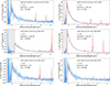 |
Fig. A.1. Fits of high confidence sample sources. Just as in Figure 3 The orange line represents the high fesc fit, the magenta dashed line represents the fesc = 0. The grey shaded area represents the region masked when performing the fit. |
Properties of the high confidence sample.
All Tables
All Figures
|
Fig. 1. Distribution of MUV as function of redshift for the whole sample. The high confidence sample (see Section 3.3) is highlighted with diamond markers, while the parent sample of spectroscopic redshifts is shown as dots. |
| In the text | |
|
Fig. 2. Top: spectrum of a model galaxy with various fesc. The model galaxy is at z = 6 and has a mass of M* = 109 M⊙, metallicity of Z = 0.05 Z⊙, ionization parameter of log U = −2, constant star formation switched on at 5 Myr, and dust modelled via the Calzetti (Calzetti et al. 2000) dust curve with Av = 0.2. As fesc increases, the βUV slope becomes steeper due to reduced nebular continuum emission, and the emission lines become weaker. The continuum emission is also affected as its nebular component scales with fesc. The full spectrum thus contains information on the escape fractions, which we exploited to constrain the fesc of galaxies with NIRSpec spectra. Bottom left: zoomed-in view of Hα. Bottom right: zoomed-in view of Hβ+[O III]. |
| In the text | |
|
Fig. 3. Example galaxy with Bayes factor > 100. Top: observed spectrum (blue line) and the two models, one with high fesc (solid orange line) and one with fesc = 0 (dashed magenta line). The shaded gray region represents the masked area. A clear difference between the two models can be seen in the βUV part of the spectrum, where the high fesc solution fits the data much better than the other solution. Middle: difference between two models highlighting the difference in the βUV slope and to some extent in the emission-line strengths. Bottom: Comparison of SFH for the two models. The models are extremely different, as reproducing the weak lines and steep βUV slope without fesc is only possible with a recent quenching of star formation. This indicates a degeneracy between SFH and fesc, which is discussed further in Section 7. |
| In the text | |
|
Fig. 4. Results of recovery simulation. The open markers indicate a Bayes factor of < 100, while the filled markers indicate a Bayes factor of > 100. The dashed black line indicates the 1:1 line, i.e., the true values. Our method can recover the high-fesc galaxies with a high confidence at all signal-to-noise levels, while we can also recover lower fesc values at high S/N levels. |
| In the text | |
|
Fig. 5. βUV slope versus EW0 of Hβ, color-coded by fesc. The parent sample is shown as circles, and the high-confidence sample is highlighted with diamond markers. All of the high-confidence sources occur at a low βUV slope, with most having a βUV slope of < − 2.5, but they span the entire EW range. |
| In the text | |
|
Fig. 6. fesc versus βUV slope. The darker diamond points highlight the high-confidence sample, while the dots represent the parent sample. The squares represent the average fesc in βUV bins, calculated from the parent sample. The fesc − βUV relation from Chisholm et al. (2022) is shown as the dashed line, with the uncertainty shown as the shaded area. With the dotted line, we show the results of Jaskot et al. (2024a), using the LyCsurv code (Flury et al. 2024). The average fesc decreases as the βUV slope becomes bluer. |
| In the text | |
|
Fig. 7. Top: fesc versus MUV. The parent sample is shown with the pink dots, the high-confidence sample is shown by the dark diamonds, and the average fesc in bins of MUV is shown as the black squares. The mean fesc does not show a trend with MUV. The average fesc of our sample is consistently measured between 10 and 15% in all bins. Bottom: fraction of sources with fesc > 0.1 in each UV magnitude bin. This fraction also shows no trend with MUV. |
| In the text | |
|
Fig. 8. Empirical cumulative distribution function (CDF) of fesc in the parent sample. The solid dark pink line shows the CDF for our data, with the shaded area representing the 95% confidence interval. The dotted lines with the shaded areas show the CDF of different simulations, including SPHINX and OBELISK, with the respective 95% confidence interval. The dashed blue lines show the three realizations of the SPICE simulation. The dot-dashed purple line represents a simple exponential distribution with a mean of 10%, as justified by the results of Figure 7, and which fits our CDF rather well. All models consistently predict mostly low-fesc objects, with a few high-fesc sources that drive the mean fesc to non-negligible values. |
| In the text | |
|
Fig. 9. Top: comparison of specific SFR distribution between the parent sample (light pink) and the high-confidence sample (dark pink). Bottom: comparison of age distribution between the parent sample and the high-confidence sample. The high-confidence sample is both more star forming and younger, indicating a relation between these properties and LyC leakage. |
| In the text | |
|
Fig. 10. Relation between fesc and O32, with the average fesc shown as black squares, in bins on log(O32). The diamond points represent the high-confidence sample, and the dots show the parent sample. The dashed gray line shows the relation between fesc and O32 form Izotov et al. (2018a). The gray triangles indicate lower limits on the O32 ratio for the points with S/N([O II]) < 3. Our points show no strong trend between ⟨fesc⟩ and O32. |
| In the text | |
|
Fig. 11. fesc versus star formation rate surface density. The high-confidence sample is shown with the dark diamonds, and the average fesc is shown with the black squares. Our sample does not show any significant trend of higher fesc with higher ΣSFR, as was expected from the proposed relation from Naidu et al. (2020) that is shown as the dashed line. |
| In the text | |
|
Fig. A.1. Fits of high confidence sample sources. Just as in Figure 3 The orange line represents the high fesc fit, the magenta dashed line represents the fesc = 0. The grey shaded area represents the region masked when performing the fit. |
| In the text | |
Current usage metrics show cumulative count of Article Views (full-text article views including HTML views, PDF and ePub downloads, according to the available data) and Abstracts Views on Vision4Press platform.
Data correspond to usage on the plateform after 2015. The current usage metrics is available 48-96 hours after online publication and is updated daily on week days.
Initial download of the metrics may take a while.