| Issue |
A&A
Volume 707, March 2026
|
|
|---|---|---|
| Article Number | A80 | |
| Number of page(s) | 23 | |
| Section | Extragalactic astronomy | |
| DOI | https://doi.org/10.1051/0004-6361/202556906 | |
| Published online | 27 February 2026 | |
SN 2024hpj: A perspective on SN 2009ip-like events
1
INAF–Osservatorio Astronomico di Capodimonte Salita Moiariello 16 80131 Napoli, Italy
2
INAF-Osservatorio Astronomico di Padova Vicolo dell’Osservatorio 5 35122 Padova, Italy
3
Dipartimento di Fisica e Astronomia “Galileo Galilei”, Università degli Studi di Padova Vicolo dell’Osservatorio 3 35122 Padova, Italy
4
Yunnan Observatories, Chinese Academy of Sciences Kunming 650216, P.R. China
5
International Centre of Supernovae, Yunnan Key Laboratory Kunming 650216, P.R. China
6
Institute of Space Sciences (ICE, CSIC), Campus UAB, Carrer de Can Magrans s/n 08193 Barcelona, Spain
7
School of Physics, University College Dublin, L.M.I. Main Building Beech Hill Road Dublin 4 D04 P7W1, Ireland
8
Institut d’Estudis Espacials de Catalunya (IEEC) 08860 Castelldefels (Barcelona), Spain
9
The Oskar Klein Centre, Department of Astronomy, Stockholm University AlbaNova 106 91 Stockholm, Sweden
10
Finnish Centre for Astronomy with ESO (FINCA), University of Turku 20014 Turku, Finland
11
Department of Physics and Astronomy, University of Turku 20014 Turku, Finland
12
Department of Physics, University of Warwick Gibbet Hill Road Coventry CV4 7AL, UK
13
Nordic Optical Telescope, Aarhus Universitet, Rambla José Ana Fernández Pérez 7, local 5 E-38711 San Antonio Breña Baja Santa Cruz de Tenerife, Spain
14
Department of Applied Physics, School of Engineering, University of Cádiz Campus of Puerto Real E-11519 Cádiz, Spain
15
Università degli Studi di Padova (UNIPD), Dipartimento di Fisica e Astronomia “G. Galilei” Via F. Marzolo 8 35131 Padova, Italy
16
INAF – Osservatorio Astronomico di Brera Via E. Bianchi 46 I-23807 Merate (LC), Italy
17
Instituto de Alta Investigación, Universidad de Tarapacá Casilla 7D Arica, Chile
18
Tuorla Observatory, Department of Physics and Astronomy, 20014 University of Turku Vesilinnantie 5 Turku, Finland
19
Cosmic DAWN Centre, Niels Bohr Institute, University of Copenhagen Jagtvej 128 2200 København N, Denmark
20
Astrophysics sub-Department, Department of Physics, University of Oxford Keble Road Oxford OX1 3RH, UK
21
Astrophysics Research Centre, School of Mathematics and Physics, Queen’s University Belfast Belfast BT7 1NN, UK
22
INAF-Osservatorio Astronomico d’Abruzzo Via M. Maggini snc 64100 Teramo, Italy
23
School of Astronomy and Space Science, University of Chinese Academy of Sciences Beijing 100049, China
24
National Astronomical Observatories, Chinese Academy of Sciences Beijing 100101, China
★ Corresponding author: This email address is being protected from spambots. You need JavaScript enabled to view it.
Received:
19
August
2025
Accepted:
23
December
2025
Abstract
Supernovae (SNe) IIn are terminal explosions of massive stars that are surrounded by a dense circumstellar medium (CSM). Among SNe IIn, a notable subset is the SN 2009ip-like, which exhibits an initial, fainter peak attributed to stellar variability in the late evolutionary stages, followed by a brighter peak, interpreted as the SN explosion itself. In this context, we analysed the spectrophotometric evolution of SN 2024hpj, an object with a triple-peaked light curve and spectra typical of a SN IIn but with a complex line profile composed of broad P-Cygni features topped by narrow emissions. Comparing it with other SN 2009ip-like events in the literature, as well as with other unpublished objects (SNe 2019mry, 2022ytx, 2024uzf, and 2025csc), we identify star-forming regions as their preferred formation environment. On the other hand, the diversity of spectrophotometric features within the sample suggests that variations in CSM mass and distribution may influence the observed characteristics. We identify four sub-classes based on the luminosity and rapidity of the light curve evolution, which provides insights into possible differences in the progenitors, while a statistical analysis of their observed rate indicates progenitor masses around 25 − 31 M⊙ or lower.
Key words: supernovae: general / supernovae: individual: 2025csc / supernovae: individual: 2024uzf / supernovae: individual: 2024hpj / supernovae: individual: 2022ytx / supernovae: individual: 2022mop
© The Authors 2026
 Open Access article, published by EDP Sciences, under the terms of the Creative Commons Attribution License (https://creativecommons.org/licenses/by/4.0), which permits unrestricted use, distribution, and reproduction in any medium, provided the original work is properly cited.
This article is published in open access under the Subscribe to Open model. This email address is being protected from spambots. You need JavaScript enabled to view it. to support open access publication.
1. Introduction
Massive stars (M ≳ 8 M⊙) are thought to end their lives in terminal explosions as core-collapse supernovae (SNe) (Smartt 2009).
Among all SN subclasses, SNe IIn (Schlegel 1990) are brighter, with an average peak magnitude of ∼ − 19 mag (Nyholm et al. 2020). Their H-rich spectra show broad (v ∼ 104 km s−1) emission lines topped by narrower (v ∼ 100 km s−1) components (Smith 2017) produced in the unshocked circumstellar medium (CSM) and photoionised by shock collisions occurring in the inner CSM regions (Chugai 1991; Chugai et al. 2004). If, instead, a star is completely stripped of H before the explosion and the CSM is relatively He-rich, the SN is classified as a SN Ibn (Pastorello et al. 2015; Smith 2017). Further stripping of the He layers produces a SN Icn, in which the dominant lines are due to C and O (Gal-Yam et al. 2021).
Some SNe show a peculiar light curve, with a first peak, called ‘Event A’, that is less luminous than a SN (≲ − 14/−15 mag at peak) and has a variable duration, from a few weeks (Tartaglia et al. 2016) to months (Elias-Rosa et al. 2016). The spectra of these SNe at this time resemble those of a SN II (Filippenko 1997), with broad P-Cygni profiles. Afterwards, the light curve brightens once again in the so-called ‘Event B’, with a higher luminosity at peak and spectra typical of a SN IIn. The best-studied case is SN 2009ip (e.g. Smith et al. 2010; Pastorello et al. 2013; Fraser et al. 2013; Mauerhan et al. 2013; Prieto et al. 2013; Graham et al. 2014; Margutti et al. 2014; Smith et al. 2014, 2022).
SN 2009ip was first discovered in 2009 (Maza et al. 2009) and classified as a SN impostor, specifically a luminous blue variable (LBV) outburst, due to its faint magnitude (M = −13.7 mag) and low expansion velocity (vFWHM = 550 km s−1) (Berger et al. 2009). A progenitor was also observed in archival images, with an estimated mass of 50 − 80 M⊙ (Smith et al. 2010). The transient later experienced a phase of repeated outbursts (Drake et al. 2010) that ended in 2012, when it rebrightened with a light curve with two peaks: Event A and Event B (Drake et al. 2012; Margutti et al. 2014; Prieto et al. 2013). After the main Event B peak, a series of smaller fluctuations was also observed during the subsequent evolution (Fraser et al. 2013; Margutti et al. 2014; Graham et al. 2014). Their explanation remains uncertain, as such features are not usually observed in SNe IIn; possible scenarios include interaction with asymmetric CSM (Graham et al. 2014) or binary interaction (Soker & Kashi 2013; Kashi et al. 2013), the latter being further supported by their periodicity (Martin et al. 2015). The left panel of Fig. 1 shows the light curve evolution of SN 2009ip over six years from first discovery, while the right panel shows a sequence of selected spectra from key phases. Spectra taken during the 2009–2010 outbursts show Balmer and He I lines with relatively slow bulk velocities (varying with eruption phase but always below 6000 km s−1), whereas broad (∼12 000 km s−1) absorption features similar to a SN II appear in spectra taken at the end of 2011 and subsequently increase with the onset of Event A in 2012 (Smith & Mauerhan 2012; Pastorello et al. 2013). In contrast, spectra of Event B closely resemble those of SNe IIn (Pastorello et al. 2013; Graham et al. 2017), although no transition to a nebular spectrum was observed (Fraser et al. 2013). The fate of SN 2009ip has been debated: while some authors argued that it terminally exploded in 2012 (Mauerhan et al. 2013; Prieto et al. 2013), the absence of newly synthesised material raised doubts about the occurrence of an actual explosion (Fraser et al. 2013; Margutti et al. 2014; Fraser et al. 2015; Pessi et al. 2023). Hubble Space Telescope (HST) photometry obtained at late times showed that the transient had faded below the original progenitor, a strong indicator of a terminal explosion (Smith et al. 2022), although it remains possible that the pre-2009 images captured the progenitor during an outburst and thus the star may not have exploded. Following the notable case of SN 2009ip, other SNe IIn have shown similar evolutions, including SNe 2010mc (Ofek et al. 2013) (which also exhibited smaller light curve fluctuations), 2011fh (Pessi et al. 2022), 2015bh (Elias-Rosa et al. 2016; Thöne et al. 2017), 2016jbu (Kilpatrick et al. 2018; Brennan et al. 2022b), and 2023ldh (Pastorello et al. 2025), as well as transitional SNe IIn and Ibn such as SN 2021foa (Reguitti et al. 2022; Farias et al. 2024; Gangopadhyay et al. 2024). Although post-explosion HST images show that some of these have effectively disappeared (2015bh, Jencson et al. 2022; 2016jbu, Brennan et al. 2022a), it is reported that the progenitor of 2011fh has not exploded (Reguitti et al. 2024).
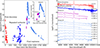 |
Fig. 1. Light curve and spectra of SN 2009ip. Left: Annotated R light curve showing the first outburst that marked the discovery of the transient in 2009, repeated outbursts during 2010 and 2011, and the main event in 2012. The inset zooms in on the latter, highlighting the presence of Events A and B. Different colours indicate the various light curve phases. Adapted from Pastorello et al. (2013). Data from Maza et al. (2009), Smith et al. (2010), Foley et al. (2011), Mauerhan et al. (2013), Fraser et al. (2013), Pastorello et al. (2013), Prieto et al. (2013), Margutti et al. (2014). Right: Selected spectra of SN 2009ip for key light curve phases (first discovery, repeated outbursts, Event A, and Event B). Numbers next to the spectra are computed from the epoch of first discovery. Data from Pastorello et al. (2013), Fraser et al. (2013). |
The mechanism generating the two events of SN 2009ip-like SNe is also disputed. For many SNe, including 2009ip, Event A is interpreted as the result of pre-explosion outburst activity, and Event B as the actual SN explosion (Pastorello et al. 2013; Elias-Rosa et al. 2016; Tartaglia et al. 2016). It is also possible that a faint SN explosion is responsible for Event A, while Event B is almost entirely due to the ejecta-CSM interaction. This interpretation was proposed, for example, in the case of SN 1996al (Benetti et al. 2016), based on light curve modelling, although Event A was not observed in that case. Alternative scenarios, such as binary interaction (Soker & Kashi 2013; Brennan et al. 2025), have also been proposed. Mergerbursts result from accretion onto a compact object in a binary system, possibly during common-envelope evolution (Chevalier 2012). Repeated passages to the periastron may trigger mass-loss episodes and outbursts (Kashi et al. 2013), whereas accretion onto a compact object during an outburst can power the luminosity sufficiently to reproduce the typical evolution of Event A (Tsuna et al. 2024a). The final explosion following the merge then produces the interaction-powered transient observed during Event B (Tsuna et al. 2024b). More recent observations of SN 2009ip-like objects support their origin from intermediate-mass (17 − 20 M⊙) progenitors, possibly in binary systems (e.g. Brennan et al. 2022c; Kilpatrick et al. 2018; Brennan et al. 2025).
In this paper, we present the results of our follow-up campaign for SN 2024hpj, a SN 2009ip-like with a light curve composed of a dimmer Event A, a subsequent brighter Event B, and a secondary dimmer peak after Event B, plus SN IIn spectra showing a composite emission profile. The paper is organised as follows: in Sect. 2 we present the observations and data reduction procedures, in Sect. 3 we analyse the spectrophotometric evolution of SN 2024hpj, and in Sect. 4 we compare it with other SN 2009ip-like objects and their host environments. We discuss the results in Sect. 5 and draw conclusions in Sect. 6.
2. Observations and data reduction
SN 2024hpj (also known as PS24dff, GOTO24bjv, ATLAS24gww, and ZTF24aaleeji) was first discovered by Rehemtulla et al. (2024) on 30 April 2024 (MJD 60430.9) at a magnitude of 20.0 mag in the g band of the Zwicky Transient Facility (ZTF; Bellm et al. 2019; Graham et al. 2019; Masci et al. 2019). The last reported non-detection was also by ZTF, at mg = 19.9 mag on 23 April 2024, seven days before the first detection. It was classified as a SN IIn on 11 May 2024 (Pérez-Fournon et al. 2024a). Its coordinates are α = 17:48:47.759, δ = +37:13:02.01 [J2000], and it is located 2 49 N, 2
 10 E from the centre of the host galaxy, WISEA J174847.58+371259.4 (a.k.a. GALEXASC J174847.58+371259.4, Cutri et al. 2013). The SN position is indicated on the finding chart shown in Fig. 2.
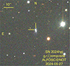 |
Fig. 2. Finding chart for SN 2024hpj, observed on 27 May 2024 with NOT/ALFOSC in the g, r, and i bands. |
2.1. Photometry
We obtained photometry of SN 2024hpj using proprietary time at the Schmidt and Copernico telescopes of the Asiago Observatory1 of the Istituto Nazionale di Astrofisica (INAF, Italy); at the Telescopio Nazionale Galileo (TNG)2 and the Gran Telescopio CANARIAS (GTC)3, both located in La Palma (Spain); and at the 2.2m telescope of the Calar Alto Observatory (CAHA-2.2) in Andalucía (Spain). We also used time allocated to the Nordic Optical Telescope (NOT)4 in La Palma (Spain) through the international collaboration Nordic-Optical-Telescope Un-biased Transient Survey (NUTS2)5. We also retrieved publicly available data from ZTF, the Panoramic Survey Telescope and Rapid Response System (Pan-STARRS; Chambers et al. 2019), and the Asteroid Terrestrial-impact Last Alert System (ATLAS; Tonry et al. 2018; Smith et al. 2020).
Pre-reduction of photometric data was performed using standard techniques in IRAF6 together with various Python packages, notably astropy (Astropy Collaboration 2022) and affiliated packages (astroquery, ccdproc, and photutils). The initial steps included removing the detector signature through bias and flat-field corrections. Following this, a cosmic-ray rejection algorithm7 was applied to further clean the data.
Astrometric and photometric calibration, as well as SN magnitude measurements, were conducted using routines from the ecsnoopy package8. When the SN was too faint (below ∼18 mag9), template subtraction was applied to the observed frames to reduce host-galaxy contamination. Archival reference images from Pan-STARRS were used to create the host galaxy templates. With ecsnoopy, the template images were aligned with the pixel grid of the science images, and hotpants (Becker 2015) was then used to convolve them, ensuring a consistent PSF and photometric scale. If no source was detected above a threshold of 2.5 times the background noise, a corresponding upper limit was registered.
Instrumental magnitudes (or upper limits) were calibrated using photometric zero points derived from local stars, with photometry from Pan-STARRS. For near-infrared (NIR) observations, the same reduction process was applied, with an additional sky-background subtraction step achieved by median-combining dithered images in each filter. Nightly zero points were established using photometry from the Two Micron All-Sky Survey (2MASS; Skrutskie et al. 2003) catalogue. The measured magnitudes are plotted alongside forced-photometry measurements from publicly available ZTF, ATLAS, and Pan-STARRS data in Fig. 3 (measurements are available online only, see the Data availability section for details). We were provided with the Pan-STARRS photometry from the Pan-STARRS Search For Transients from the ongoing Pan-STARRS NEO survey (Fulton et al. 2025). Detections exist in the y and w band, but no historic detections were found on approximately 60 nights between MJD = 57448 and 60234 through forced photometry.
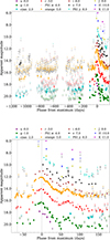 |
Fig. 3. Apparent light curve of SN 2024hpj in the u, g, r, i, z, J, H, K, cyan, orange, w, and y bands. A rigid shift is applied for better visualisation. Top: Complete light curve covering the last ∼3 years. Bottom: Zoom-in on the Event A+B light curve. Dashed grey lines indicate the peaks of Events A and B, while grey arrows and open symbols indicate upper limits. Phases are calculated with respect to the epoch of the Event B maximum (MJD 60455). |
2.2. Spectroscopy
Optical spectra were acquired with the Alhambra Faint Object Spectrograph and Camera (ALFOSC) at NOT, the Device Optimized for the Low Resolution (DOLORES) at TNG, the Calar Alto Faint Object Spectrograph (CAFOS) at CAHA-2.2, and the Optical System for Imaging and low-Intermediate-Resolution Integrated Spectroscopy (OSIRIS+) at GTC.
The same data reduction procedure was applied to all spectra. Using standard IRAF tasks, we corrected the 2D images for bias and flat-field and subtracted cosmic rays. We then extracted the SN trace and calibrated in wavelength using spectra of standard lamps, and in flux with the spectrum of a spectrophotometric standard star. For spectra obtained with ALFOSC and OSIRIS+, the procedure was automated using the foscgui pipeline10. Finally, spectra were rescaled in flux to match the host-subtracted photometry at the corresponding epochs. A log of all spectral observations is available online (see the Data Availability section), while the complete spectral sequence is plotted in Fig. 4.
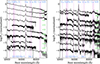 |
Fig. 4. Spectral evolution of SN 2024hpj, with all spectra corrected for redshift and reddening. Numbers next to each spectrum indicate the rest-frame phase since the Event B maximum in the g band. Dotted lines indicate the position of major emission lines. |
2.3. Redshift and reddening
We measured the average position of the narrow Hα emission present in the SN spectra and derived a redshift z = 0.0187 ± 0.0003. Adopting the cosmology H0 = 73 km s−1 Mpc−1, Ωm = 0.27, and Ωvacuum = 0.73 from Tully et al. (2013), we obtain a distance d = 74 ± 1 Mpc, corresponding to a distance modulus m − M = 34.36 ± 0.03 mag. From the Nasa Extragalactic Database (NED)11, we find an absorption AV = 0.08 ± 0.01 mag in the SN direction. Adopting RV = AV/E(B − V) = 3.1 (Cardelli et al. 1989; Schlegel et al. 1998), we derive E(B − V) = 0.020 ± 0.003 mag for the Galactic reddening. We do not detect any Na I D lines in the SN spectra associated with the host galaxy. For this reason, hereafter we assume a negligible contribution of the host galaxy to the total reddening towards SN 2024hpj.
3. Evolution of SN 2024hpj
3.1. Light curve
Figure 3 shows the multiband light curve of SN 2024hpj. The light curve shows a peculiar shape, with a first low-luminosity peak (Event A) that reaches an apparent magnitude in the ATLAS orange band o = 19.8 ± 0.1 mag (absolute magnitude Mo = −14.5 ± 0.2 mag) when fitted with a polynomial function. Constraining the start of this phase is challenging due to its faint apparent magnitude, but it appears to last at least 20 days. The first peak is followed by a second, brighter peak (Event B). The last declining point of Event A and the first rising point of Event B are separated by a gap of 13 days. Assuming that the first point after the gap marks the start of the rise to the second peak, the time to maximum is 37 ± 1 days, which is longer than expected for regular SNe II but consistent with interaction-powered SNe. The maximum luminosity reached is mo = 17.11 ± 0.02 mag (Mo = −16.32 ± 0.04 mag), occurring on MJD 60454 ± 1 days. This epoch is adopted as the reference for the peak throughout the paper. The subsequent decline is slower than the rise, lasting about 50 days, after which the luminosity increases again in all bands, forming an ulterior peak that reaches a maximum luminosity of o = 19.18 ± 0.02 mag (Mo = −15.13 ± 0.04 mag) 67 days after the Event B peak. Finally, the light curve declines slightly more slowly than the 56Co decay timescale, until the SN is lost due to solar conjunction.
We also calculated a pseudo-bolometric light curve. Magnitudes were converted to flux densities using photometric zero points12. The flux within the sampled spectral region was integrated using the trapezoidal rule, assuming zero flux outside the boundaries of the bluer and redder filters and constant colour evolution between contiguous data points. The flux was then converted to luminosity based on the distance modulus. Figure 5 shows the resulting light curve. By fitting the late-time tail with a linear decline and comparing its slope to that of SN 1987A (Arnett & Fu 1989), we derive an upper limit for the 56Ni mass of 0.07 ± 0.01 M⊙. We caution that, as noted above, the decline is slightly shallower than expected for 56Co decay alone, and interaction may still contribute significantly to the energy budget. Although the derived 56Ni mass is almost identical to that of SN 1987A, the main peak of SN 2024hpj is significantly brighter, indicating that the interaction provides an additional source of energy.
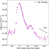 |
Fig. 5. Pseudo-bolometric light curve of SN 2024hpj, constructed by integrating the u to K bands. The expected theoretical decay rate due to 56Co is also shown. |
Aside from the general declining trend, the light curves (both multiwavelength and pseudo-bolometric) exhibit several bumps beyond the main peaks already discussed, which are likely due to interaction with the CSM. To further investigate this, we applied the procedure described by Martin et al. (2015). In short, we fitted the peak and the decline with two second-order polynomial functions: one between −20 and 25 days from the peak and the other between 25–45 and 90–200 days after the peak, thereby excluding the secondary bump. This fit, shown in Fig. 6, was then subtracted, and the residuals are plotted in Fig. 7. The secondary peak around 50–100 days is the main feature, while the remaining residuals are scattered around zero. Excluding the secondary peak, which was not fitted, the variation is higher in the early light curve, with undulations peaking around 0 and +25 days in all bands, as well as in the pseudo-bolometric light curve. Larger variations around 50 days, particularly in the g band, are due to poor fitting of the epochs immediately preceding the secondary bump, as shown in Fig. 6. Smaller residual structures at earlier epochs may indicate that the CSM traversed by the ejecta had either changes in density (possibly even multiple distinct shells) or a non-spherical shape (Kurfürst et al. 2020).
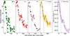 |
Fig. 6. Fit of the peak (dotted blue line) and decline (dashed cyan line) of the multiband (g, r, i and orange) and pseudo-bolometric light curves. The secondary bump is excluded from the fit (see text). |
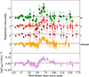 |
Fig. 7. Residuals of the multiwavelength (upper panel) and bolometric (bottom panel) light curves after subtracting the peak and decline fits. Magnitudes are shifted for better visualisation. The dashed lines indicate the mean value of the residuals for each band. |
3.2. Spectra
Figure 4 shows the spectral sequence of SN 2024hpj. We did not obtain any spectra during Event A. The first spectrum, taken nine days before the Event B maximum, exhibits a blue continuum and prominent broad P-Cygni profiles in Hα and Hβ, with a hint of a blue shoulder that may be a proxy of the H shell. The broad lines are superimposed by narrow emission lines with full width at half maximum (FWHM ∼ 600 km s−1, corrected for instrumental broadening) originating from the ionised CSM surrounding the SN. The spectrum at −3 days is similar but shows deeper P-Cygni absorptions, with He Iλ5876 also detected in emission at this phase. Spectra at +5 and +12 days show enhanced P-Cygni profiles from Hγ and Hδ, along with a cooler continuum. At +22 days, we detect P-Cygni absorption features indicating several Fe II lines, along with broad emission corresponding to the Ca II NIR triplet λλλ8498, 8542, 8662. The spectra remain similar until +76 days, with increasing contributions from Fe II multiplets in the bluer part of the spectrum and Ca II NIR in the redder part, plus [O III] λλ4959, 5007 from either the host galaxy or the CSM itself. We cannot exclude the contamination from other host lines such as Hα, [N II] λλ6548, 6583, and [S II] λλ6716, 6731, which, although not detected, could be blended with the broad Hα from the SN. At +89 days, we detect blended emission lines from [Ca II] λλ7293, 7326, along with a double-peaked emission that we tentatively identify with He Iλ7065. Around 100 days after maximum, the P-Cygni absorptions disappear, and the emission lines show electron-scattering profiles.
Figure 8 shows the evolution in velocity space for Hα and Hβ (first two panels). Both lines show similar evolution, with a broadening of the feature closer to the peak and a considerable shrinkage shortly thereafter. We also fitted the broad emission lines with a Gaussian function to estimate the flux, and the resulting  flux ratio is shown in the third panel of Fig. 8. There is an evident evolution from values close to or below the 3.1 limit for case B hydrogen recombination (Osterbrock & Ferland 2006) to significantly higher values, indicating a probable collisional origin for the excitation.
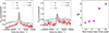 |
Fig. 8. Evolution of Hα and Hβ during the first month after discovery. Left: Evolution of Hα in velocity space. Centre: Evolution of Hβ in velocity space. Numbers indicate the phase from the peak. Right: Flux ratios of |

We fitted a blackbody (BB) function to the spectral continuum to estimate its temperature and to derive the corresponding radius and luminosity. For accuracy, we excluded areas in the vicinity of major emission lines (Hα and Hβ) from the fit. Spectra at +12, +29, and +69 days were excluded because the limited wavelength coverage does not allow for a good fit of the continuum. The results are shown in Fig. 9. The temperature decreases rapidly during the first ∼60 days from the peak of Event B, decreasing from 10 000 to 5000 K. The evolution of BB luminosity is straightforward, showing an initial plateau in the first three spectra followed by a sharp decline. The radius shows a more erratic behaviour, initially increasing in the first spectra before decreasing, although later than the luminosity and the temperature. A slight increase in the radius may correspond to the hint of plateau observed before the decline in the light curve; however, there is no evident variation in correspondence with the second bump of the light curve. This behaviour is likely a fluctuation due to a poor fit of the spectrum. A secondary peak is also observed at approximately +70 days. This feature corresponds to smaller increases in the temperature and luminosity, indicating that the CSM responsible for the interaction is producing additional heat, shifting the continuum peak towards the blue, while the BB radius expands to the position at which interaction is taking place. We did not perform the fit on later spectra because the assumption of BB emission no longer holds at late stages in the evolution (a fit on the pseudo-bolometric light curve confirms this assumption).
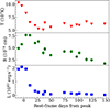 |
Fig. 9. Temperature, radius, and luminosity from the blackbody (BB) fit to the spectra. There is a clear decline during the first ∼60 days, while the data show a highly variable trend, likely indicating that the assumption of a BB is no longer valid. |
To estimate the expansion velocity of the ejecta, we measured the position of the minimum of the P-Cygni absorption on Hα, He Iλ5876, and Fe IIλ5169 (Fig. 10). The velocity of He Iλ5876 decreases at all epochs, although we cannot exclude some contamination from Galactic Na I D. The behaviour of Fe II is more erratic, with an increase around the second peak of the light curve, which could be attributed to scattering. Moreover, this line shows the largest scatter, possibly because of the difficulty of identification in some spectra. The Hα line shows the most peculiar evolution, with an initial slow decrease during the first three spectra, followed by a rapid drop and then a flattening that settles into a plateau at the onset of the second peak, with a possible increase near its maximum at around +70 days. The differing behaviour of the expansion velocities measured on different spectral lines is probably because these lines originate from different regions of the ejecta, particularly if the photosphere is detached and the faster spectral lines are far above it. This phenomenon manifests as a flattening of the expansion velocity (Arcavi et al. 2017), as seen here for Hα. In this scenario, Hα follows the outer layers, while Fe II traces the photosphere. Adopting ∼10 000 km s−1 as the average photospheric velocity during the secondary peak returns a radius of ∼3 × 1014 cm, of the same order of magnitude as that derived from the BB fit (see Fig. 9).
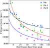 |
Fig. 10. Expansion velocity measured from the minimum of the broad P-Cygni for Hα, He Iλ5876, and Fe IIλ5169, together with the corresponding power-law fits (black, red, and blue lines, respectively). A similar double trend is seen for Hα before and after phase +30 days, while He I follows a power-law decline, although, it is contaminated by Na I D, especially at late phases. The Fe II line also shows a power-law decline, albeit with some scatter, possibly due to the difficult identification. |
We do not detect any narrow (FWHM ∼ 100 km s−1) P-Cygni profiles in the spectra, likely because the resolution is insufficient to resolve this faint feature or because of the viewing angle; therefore, we do not have a clear measure of the wind velocity of the progenitor. We therefore analysed the spectra with the highest resolution, obtained at +12 and +29 days from the Event B peak, and measured the FWHM of the narrow Hα emission line. The measured values are 4.81 Å and 4.75 Å, respectively (corresponding to 5.47 Å and 5.51 Å before correcting for resolution). The average of the two values translates to an upper limit on the wind velocity of 220 ± 30 km s−1. This value is significantly higher than the few tens of km s−1 expected for a red supergiant (RSG) progenitor, but is consistent with values inferred for other SN 2009ip-like events (e.g. 2009ip itself, for which a wind velocity of 550 km s−1 was derived; Moriya 2015). This provides an upper limit on the wind velocity that carried the CSM to its position at the time of the explosion. The expansion velocity at the onset of the second bump, occurring approximately 50 days after the main peak, is ∼15 000 km s−1 (derived by fitting the expansion velocity from the P-Cygni minima with a power-law decline). We can then estimate that the CSM shell responsible for this bump was ejected approximately 1.8 years before the explosion.
4. SN 2009ip-like objects
To study the SN 2009ip-like subclass, we assembled a sample of similar objects. The primary criterion for assigning a SN to this class is the presence of Event A. However, such an event may be missed due to its relative faintness (particularly for more distant objects) or its duration (especially for those lasting only a few days). A practical approach to address this issue is to examine both the light curve and the spectra. SN 2009ip-like objects exhibit spectra during Event B that resemble those of SNe IIn, with prominent narrow emission lines. In contrast, their light curves are similar to those of regular SNe IIL (Barbon et al. 1979), with average peak magnitudes (M ∼ −18) and duration, which fades some 100 days after the peak. Applying these criteria, we compiled a sample of 24 comparison SNe: 19 from the literature and five unpublished objects observed by our group. We briefly introduce the latter and summarise their characteristics. The light curve and spectra of these objects are shown in Figs. 11–12 (photometric measurements and spectral logs are provided online; see the Data availability section), while their main properties are summarised in Table 1.
-
SN 2019mry: Event A is poorly constrained, but there is a first rise to a peak of approximately −14.4 ± 0.2 mag in the I band about 30 days before the peak of Event B, which reaches MI = −17.5 ± 0.2 mag. The light curve then declines over the following 30 days at a rate of 0.0061 ± 0.0007 mag d−1, before setting on a plateau that lasts roughly 20 days. The decline then resumes at a slightly slower pace of 0.0046 ± 0.0002 mag d−1. All spectra of SN 2019mry were obtained after the Event B peak. A Hα with a significant P-Cygni profile dominates at all epochs. The narrow component also shows P-Cygni absorption, from which we measure a velocity of almost 2000 km s−1. A strong absorption, sometimes accompanied by a less evident emission, is also present at all times at the position of He Iλ5876. The Ca II NIR appears in the spectrum at +26 days.
-
SN 2022mop: The light curve of this SN is unusual, showing activity from multiple outbursts over three years prior to the explosion (Srivastav et al. 2025; Sollerman et al. 2025). Event A peaks at −15.16 ± 0.02 mag in the r band, 26 days before the peak of Event B, which reaches −18.40 ± 0.02 mag. The available spectra were obtained during the rise to Event B. These spectra are blue and dominated by Balmer emission lines with symmetric, electron-scattering profiles. Brennan et al. (2025) recently highlighted similarities between SNe 2022mop and 2009ip, proposing a merger-burst scenario to explain the two peaks. In this scenario, the progenitor of SN 2022mop belongs to a binary system in which the companion star strips the progenitor, which subsequently explodes as a stripped-envelope SN (SESN). The neutron star (NS) remnant from the explosion enters an eccentric orbit due to natal kicks and interacts with the inflated companion and the previously-emitted CSM. This interaction is periodic and thus explains the variability witnessed between the first burst in 2022 and Event A+B in 2024–2025. Drag forces then decrease the orbital period until an in-spiral occurs, producing a merger that powers Event B rebrightening.
-
2022ytx: The r light curve peaks at −17.862 ± 0.004 mag, with a short plateau 17 − 36 days after the Event B peak. Detections of Event A are observed starting approximately 60 days before the Event B peak in the ATLAS cyan and orange bands and peaking 20 days after at ∼ − 15 mag in the orange band. Although initially classified as a SN IIb with precursor activity (Srivastav et al. 2022), a more careful analysis of the dataset allows us to classify this object as a peculiar Type IIn SN, sharing similarity with SN 1996al (Benetti et al. 2016). The spectra of SN 2022ytx resemble those of SN 2024hpj, with the same composite structure in the Hα profile. This SN also shows a narrow P-Cygni profile in the Hα, with a calculated velocity of ∼1000 km s−1.
-
2024uzf: Event A in this SN is relatively bright, peaking at −15.70 ± 0.01 mag in the r band, 33 days before Event B, which peaks at −18.21 ± 0.01 mag. The light curve then declines rapidly at 0.042 ± 0.002 mag d−1 until a brief plateau appears between 53 − 62 days, after which the SN is lost due to a sudden luminosity drop. We obtained all spectra around the Event B peak. These spectra resemble those of typical SNe IIn, with blue continua and Balmer emission lines with electron-scattering profiles.
-
2025csc: Event A in the light curve of SN 2025csc is suggested from ATLAS stacked data; however, ZTF only provides detection limits at similar epochs, casting doubt on the reliability of the ATLAS detections. To verify this, we performed PSF photometry on ZTF images taken around the time of Event A (from MJD 60706 to 60729) and find one detection at 20.371 ± 0.149 mag within 1σ of the ZTF limit magnitude in the r band on MJD 60725. If real, Event A resembles SN 2024uzf in shape but is brighter, peaking at −16.23 ± 0.04 mag in the orange band, 31 days prior to Event B. The latter, instead, is almost identical to SN 2024hpj, reaching −18.05 ± 0.04 mag. We obtained all spectra around and after the maximum of Event B. The main feature is an asymmetric Hα with a narrow P-Cygni profile that returns a velocity of ∼800 km s−1. In the final spectrum at +93 days, Ca II NIR also appears, along with He Iλ5876 and numerous Fe II lines. Notably, we observe O Iλ8446 in emission in all spectra, whereas O Iλ7774 appears only as weak absorption. This could be interpreted as an effect of Bowen fluorescence (also known as UV pumping, Osterbrock & Ferland 2006): the Lyβ λ1025.72 and the O Iλ1025.76 lines are in resonance and this pumps electrons from O I to higher levels. The subsequent de-excitation produces O Iλ8446 emission but not O Iλ7774. This mechanism has been observed in intermediate-luminosity red transients, which exhibit light curves similar to faint, linearly declining SNe II and progressively redder spectra (e.g. Cai et al. 2021). In this context, Valerin et al. (2025) determined that the Doppler shift required for perfect wavelength alignment is +12 km s−1, with H and O moving in opposite directions. Furthermore, the Bowen mechanism appears more efficient at later phases, when opacity is lower and Lyβ photons have fewer opportunities to thermalise before encountering O I (Valerin et al. 2025). The Bowen mechanism should also produce O Iλ11287, therefore detecting this line would confirm our hypothesis. Our spectra lack the wavelength coverage to confirm this; nevertheless, the interpretation remains plausible, and follow-up observations at NIR wavelengths would help to confirm it.
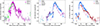 |
Fig. 11. Light curves of objects observed in our sample. Each SN is shown in the best-sampled broadband light curve. Comparisons with SN 2024hpj and, when available, SN 2009ip, are also included. Phases are calculated from the Event B peak. The luminosity at this peak and the subsequent decline rate are very similar, whereas there is some variation in the duration and brightness of Event A. Arrows and open symbols indicate upper limits. |
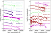 |
Fig. 12. Spectral evolution of objects observed in our sample. All spectra are redshift- and reddening-corrected and rescaled for better visualisation. Numbers close to the spectra indicate the rest-frame phase from the Event B peak. |
Summary of properties for the SNe observed in this study.
4.1. Comparison with supernovae from the literature
As described above, we performed a literature search to select all SNe showing possible Event A + Event B light curves. To account for the fact that Event A may be missed prior to the SN discovery, we also considered other SNe IIn with spectra that match those of SN 2024hpj and 2009ip13. Additionally, SNe 2019mry, 2002ytx, and 2025csc show clear narrow P-Cygni profiles on top of broader emission. We therefore included historical SNe that display the same structure and similar Event B evolution, assuming that Event A was missed due to limited survey coverage (e.g. SNe 1994aj Benetti et al. 1998, 1996L Benetti et al. 1999, 1996al Benetti et al. 2016, and 2000P Cappellaro et al. 2000). Notably, several of the SNe that exhibit this emission profile also showed evidence of pre-SN eruptions, similar to SN 2009ip (e.g. iPTF13z Nyholm et al. 2017 and 2013gc Reguitti et al. 2019). The selected SNe are reported in Table 2, together with the main characteristics of their host galaxies.
Host-galaxy characteristics of sample SNe.
To compare their light curves, we computed pseudo-bolometric light curves by integrating the flux across all available bands as described in Sect. 3.1, using the distance modulus reported in the corresponding references. For the unpublished SNe, we applied the same cosmology as for SN 2024hpj (see Sect. 2.3) and included any available host-galaxy reddening. For each SN, we used the information from all available filters. Because the filter coverage differs significantly among the comparison SNe, ranging from full UV–NIR coverage to only a few filters, we constructed the pseudo-bolometric light curve of SN 2024hpj to match, in each case, the available photometry of the comparison SNe. Figure 13 displays the pseudo-bolometric light curves for all selected SNe compared to that of SN 2024hpj. In each panel, we also report the wavelength range used to build the pseudo-bolometric light curve.
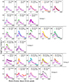 |
Fig. 13. Individual pseudo-bolometric light curve of SN 2024hpj (mauve points) compared with the sample SNe. All light curves are matched at the Event B peak (for SN 2022mop, only the 2024–2025 period is shown). Labels indicate the bands used to build the light curve (see text). Four groups are discernible: rise and/or decay time and peak luminosity similar to SN 2024hpj (group 1); more luminous and/or faster declining than SN 2024hpj (group 2); slower declining than SN 2024hpj (group 3); and exhibiting a plateau (group 4). |
Figure 13 reveals four groups: SNe that are more similar to SN 2024hpj in terms of rise and/or decay times (when covered) and peak luminosity (group 1); those that are more luminous and/or decline faster than SN 2024hpj (group 2); those that are brighter and decline more slowly than SN 2024hpj (group 3); and those with a plateau (group 4). Notably, SN 2024hpj is the only object with a bright second peak after the Event B peak (although iPTF13z showed several smaller bumps, they are not as extreme as for SN 2024hpj and more similar to the undulations of SN 2009ip, rather than a distinct peak, Nyholm et al. 2017). All SNe with late-time data show late-time tails roughly consistent with powering from the decay of 56Co. However, as discussed in Sect. 3.1, the interaction can still dominate, masking the contribution of 56Ni and leading to shallower slopes and/or higher estimates for the 56Ni mass. We also caution that, in the case of SN 2009ip, the presence of 56Ni was questioned since the decline was faster than expected and the interaction was arguably the main driving mechanism (Fraser et al. 2013). This dichotomy suggests a common inner engine, with evolutionary variations most likely due to the mass and distribution of the CSM, which affects H recombination and the escape time for photons.
In SNe IIn, the observed diversity is generally due to the shape and density of the CSM, as well as the mass and velocity of the ejecta, with different combinations of these parameters generating a continuum of observed spectrophotometric properties (Ransome & Villar 2025). Nevertheless, there appears to be a bimodality in the decline time (fast versus slow; Nyholm et al. 2020; Ransome & Villar 2025), as well as in the peak energy (Hiramatsu et al. 2024). There is also a positive correlation between higher CSM masses and decline time, as well as between longer declines, slower rise times, and higher peak magnitudes, indicating that brighter SNe IIn tend to evolve more slowly and have more CSM (Ransome & Villar 2025). In the context of our sample of SN 2009ip-like events, those belonging to group 1 would share a similar progenitor with SN 2024hpj, while those in group 3 would have a more massive CSM, and those in group 4 may have a progenitor that retained a larger part of their H envelope, allowing a plateau to form. Group 2 is more challenging to interpret, as it deviates from the general rule that slower evolution produces brighter light curves. The combination of a brighter, yet faster, or equally declining, light curve relative to SN 2024hpj may indicate a different CSM density or geometry.
For the majority of the SNe in the sample, Event A shows a clear rise to a peak followed by a decline, which is followed, after a variable delay, by the rise to Event B. For these objects, we measured the main peak magnitude and duration of Event A and searched for possible correlations with the magnitude of Event B and the separation between the two peaks. Although there is a large spread, the average duration of Event A is around 20 − 40 days, and the peak of Event A occurs between 30 − 40 days from the peak of Event B. These values do not appear to be affected by the magnitude of either Event A or Event B. The only significant correlation is between the peak magnitudes of Events A and B, which is shown in Fig. 14. A brighter Event A tends to be associated with a brighter Event B, consistent with SNe IIn exhibiting progenitor activity, and has been interpreted as evidence for more massive CSM in brighter events (Ofek et al. 2014; Strotjohann et al. 2021). If interaction is a major contributor during the evolution of SN 2009ip-like events, such an explanation is plausible. This correlation is particularly evident for SNe belonging to group 1, which also display the broadest spread in magnitude and include the faintest Events A and B in the sample. Objects in group 4 (albeit only two of them showed a clearly measurable Event A+B) also follow this correlation and are among the brightest in the sample. Group 2 and 3, by contrast, cluster around average magnitudes, with group 3 showing a slight deviation from the correlation, characterised by a bright Event B associated with a fainter-than-average Event A. While these considerations are limited by the small number of objects in the sample, this diversity could be tied to the physical parameters of the progenitor and its CSM. In particular, a more massive progenitor could give rise to a brighter transients overall, whereas a larger amount of CSM ejected prior to the explosion could power a brighter Event B while not affecting Event A.
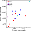 |
Fig. 14. Magnitude at the Event B peak as a function of the magnitude at the Event A peak. Measurements were performed in the r and R bands when available. For SNe not covered during Event A in r (SNe 2025csc, 2022ytx, and 2019mry), we performed the measurements in the orange band for SNe 2025csc and 2022ytx, and in the I band for SN 2019mry. Colours are the same as in Fig. 13. Error bars are present but often smaller than the data points. |
Figure 15 compares the spectral characteristics of SN 2024hpj with the selected sample SNe peak of Event B and approximately 100 days later. The spectra around the peak of Event B are markedly different within the sample: while the spectrum of SN 2024uzf is of insufficient quality to distinguish anything other than a composite Hα feature, SNe 2022ytx and 2025csc are the most similar to SN 2024hpj, with the same composite structure in the emission lines, particularly in Hα. In contrast, SN 2022mop exhibits a spectrum more closely resembling those of SNe 2009ip, LSQ13zm, and 2016bdu (respectively belonging to groups 2, 3, and 4 based on their light curve), even though its light curve is more similar to those of group 1. These spectra are hotter than that of SN 2024hpj shown here and are characterised by emission profiles dominated by electron scattering that resemble the earlier spectra of SN 2024hpj, but lacking P-Cygni absorption. Although clear differences between the SNe spectra belonging to groups 2, 3, and 4 are not apparent here, we note that SN 2009ip began to exhibit composite line profiles similar to those of SN 2024hpj approximately one week after its maximum. This indicates that the spectra of these objects evolve quite rapidly around the maximum of Event B, transitioning from higher to lower optical depth as the electron scattering profiles recede and the structure of the line beneath is revealed. The timing of the transition is likely due to the amount of material that the shock wave must traverse before it emerges. Spectra obtained at later phases, around 100 days, are instead more similar, with flat continua that indicate that the emission is no longer a BB, and with a narrower Hα. In spectra with sufficient wavelength coverage, the blended Ca II NIR triplet is always visible.
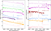 |
Fig. 15. Spectral comparison of SN 2024hpj with selected SNe from the sample. Left: Comparison around the Event B peak. Right: Comparison approximately 100 days after the Event B peak. Numbers in parentheses indicate the group based on the light curve (see text). Phases from the Event B maximum are also reported. All spectra are redshift- and reddening-corrected. |
4.2. Host galaxies
To infer the general properties of the population of the progenitors, we explored the characteristics of host galaxies. For each SN in our sample, we retrieved the host morphological classification, preferentially from HyperLeda (Makarov et al. 2014) or NED, or from reference articles, when available. In cases where no classification was available, namely for the host galaxies of SNe 2010mc, 2016bdu, 2018cnf, 2019mry, LSQ13zm, 2023vbg and 2024hpj, we estimated the morphology through a direct comparison of their images with those of galaxies with established classifications.
For the unclassified hosts, we also chose to apply spectral energy distribution (SED) fitting techniques to retrieve some intrinsic properties, primarily the star formation rate (SFR). We retrieved the UV, optical, and NIR photometry from NED assuming a 10% error on each flux (the flux values are reported in Table B.1). This assumption accounts for possible systematic errors not included in the catalogue estimates. For the host of 2019mry, we adopted Legacy Survey (Dey et al. 2019) DR10 photometry. For the hosts of SNe 2010mc and 2024hpj, we found no available photometry, therefore we modelled pre-explosion Pan-STARRS stacked images in the g, r, i, and z bands and retrieved upper limits from the 2MASS point source catalogue. The SED fitting was performed with BAGPIPES (Carnall et al. 2018) using an exponential star-formation history and a Calzetti dust extinction law (Calzetti et al. 1994). The redshift was assumed to be equal to that of the SNe. The full results of the SED fitting are summarised in Table 3. Our findings highlight that the host galaxies are generally low-mass dwarf galaxies, with the sole exception of the host of SN 2018cnf (LEDA 196096), which is a massive galaxy. Two out of five hosts are consistent with being main-sequence galaxies (the hosts of SNe 2010mc and 2018cnf), while the remaining three appear to be in a starburst phase (see Appendix B for details).
Results of the SED fitting.
The transient’s position within its host galaxy is also important for inferring the stellar population to which the progenitor belongs. We visually inspected the images of each SN and determined its position among the following categories: halo, spiral arm, disc, outskirts, or bulge, to provide a general idea of the SN environment. Figure B.2 shows the finding charts for the SNe in the sample as r band cutouts from SkyView14. In a de-projected image, a transient could be further away from the galaxy nucleus due to the inclination. We then measured the projected distance of the SN from the host galaxy centre, which provides a lower limit to the true distance. These measurements, together with the host morphological parameter t15 and the radius corresponding to a surface brightness of 25 mag (R25), are reported in Table 2. From these SNe, we built a volume-limited sample by establishing a cut at 100 Mpc (z = 0.024). Moreover, since SNe discovered before SN 2009ip were not classified as 2009ip-like, we may have missed some contributors. Therefore, SNe discovered before 2009 were excluded from the filtered sample. Figure 16 shows the distribution of the host morphology and the distance of the SNe from the centre of the host galaxy using these criteria. Although small dwarf galaxies whose morphological class was difficult to determine appear dominant in the volume- and time-limited sample, there is also a strong contribution from spiral and irregular galaxies, yielding an average of t = 5 ± 3 in the filtered sample and a 95% confidence interval of t = 3.12 − 6.49. The variation is therefore large, and no preferred morphological type is evident; however, spirals constitute the majority of hosts in the volume- and time-limited sample, suggesting a prevalence of younger stellar populations. Regarding the position of the explosion site, SNe tend to explode within a few kiloparsecs of the host centre. We caution that this measurement represents a lower limit, as the de-projected distance may be larger. Moreover, as shown in Table 2 and in the second panel of Fig. 16, the position is generally marginal, either located in a spiral arm or in the outskirts, and the majority of SNe are found well outside the bulge. Thus, the stellar populations surrounding the explosion sites are likely young and blue.
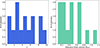 |
Fig. 16. Distribution of host morphology as a function of the t parameter and SN distance from the host-galaxy centre for SNe in the volume- and time-limited sample (within 100 Mpc, discovered after 2009). |
Classical SNe II with these absolute magnitudes and evolution timescales are associated with ∼15 − 20 M⊙ RSG stars (Boian & Groh 2020; Smartt 2009; Morozova et al. 2017). However, the environments in which the SN 2009ip-like events in our sample preferentially explode appear to indicate more massive progenitors. While older SNe (discovered before ∼2013) are mostly found in grand-design spiral galaxies, the trend with newer SNe in the sample indicates more dwarf galaxies, consistent with our SED fitting results. This could be a selection effect: in the past, SNe were discovered by chance during the observation of nearby, massive galaxies. Modern surveys, in contrast, focus more on the distant Universe and thus detect smaller galaxies that were previously overlooked because they were too faint to be reached with older instruments. However, it is noteworthy that Tartaglia et al. (2016) classified the host of LSQ13zm as a blue compact dwarf galaxy (BCDG, Haro 1956; Zwicky et al. 1961). These are blue with low luminosity and metallicity, and some display spectra characteristic of H II regions with high SFRs (Fanelli et al. 1988; Cairós et al. 2001). They could therefore be favourable hosts for this type of SNe.
5. Discussion
The progenitors of SN 2009ip-like events remain a topic of debate. While Event A is consistent with being a stellar eruption, the luminosity of Event B more closely resembles that of a terminal explosion. However, for SN 2011fh, a source is still visible at the SN position, only slightly fainter than three years before the major brightening in 2011, suggesting that the star may not have exploded (Pessi et al. 2022; Reguitti et al. 2024).
Many authors proposed LBVs as possible progenitors of SN 2009ip-like events (e.g. Kashi et al. 2013; Soker & Kashi 2013; Smith et al. 2014), as an LBV could easily produce the observed CSM during the eruptive phases, which typically occur close to the explosion. Therefore, the CSM would remain close to the progenitor, allowing interaction to commence soon after the explosion. Several mechanisms may trigger the eruptive mass-loss phases in LBVs, including stripping by a binary companion (Kashi & Soker 2010) or pair-instability processes (PI; Smith & Owocki 2006; Woosley et al. 2007). The progenitor of SN 2005gl was proposed to be an LBV (Gal-Yam et al. 2007) (although it was detected in only one filter and it was not possible to confirm its variable nature) and the SN spectra resemble those of SN 2009ip-like objects (Pastorello et al. 2018). In addition, other SN 2009ip-like events have high calculated progenitor masses (e.g. SN 2011fh has a reported progenitor mass of 35 − 80 M⊙, in line with an LBV scenario, Pessi et al. 2022, although we recall that the progenitor is likely yet to explode, Reguitti et al. 2024). However, these estimates assume that the progenitor was in a quiescent state, which is unlikely to be the case, especially when considering highly variable stars such as LBVs. If the progenitor was observed even during a minor outburst (Smartt 2015), the mass would be dramatically overestimated. Therefore, the identification of the progenitor in pre-explosion images provides only an upper limit to its mass. Moreover, LBVs may not be the only stars capable of producing a high mass-loss before the explosion, as Wolf-Rayet (WR) stars (Dwarkadas 2011) or even RSGs have been proposed as viable alternatives.
A PI-induced explosion could produce a late-time tail with a decay rate similar to that expected from a 56Ni-powered light curve (Kasen et al. 2011). However, the peak luminosities of SNe in our sample are relatively faint, far below the levels PI models predict (∼1044 erg s−1, Nagele et al. 2024). Pulsational PI (PPI) could easily explain the dense CSM ejected shortly before the explosion, as well as the shallower late-time decay discussed in Sect. 3.1. However, this scenario is not supported by the measured expansion velocity: PPI models suggest low velocities (≲5000 km s−1, Woosley 2017), whereas our measurements from several emission lines indicate velocities at least twice as high (Fig. 10). Although models of Eta Carinae expansion velocities indicate that some layers can reach > 10 000 km s−1 due to asymmetric eruptions, the average velocity of the main eruption remains < 600 km s−1 (Smith et al. 2018). Furthermore, Smith et al. (2022) examined the PPI scenario for SN 2009ip, concluding that it could not explain the series of weak ejections prior to the major burst or for the H retention observed in SN 2009ip. This contrasts with PPI models, which predict complete ejection following the first pulse. In addition, in our sample we observe that the late-time decline rate of the light curve is mostly consistent with radioactive 56Co, whereas PPI can vary and depends on the amount of mass ejected. Although a PPI SN could, in principle, mimic the late-time evolution of 56Co, it is unlikely to occur for all the SNe in the sample, since PPISNe are not expected to show a radioactive tail due to the absence of 56Co (Woosley et al. 2007).
Another progenitor scenario for SN 2009ip-like events was recently proposed for SN 2016jbu, based on HST observations suggesting a possible yellow supergiant (YSG) with 17 − 30 M⊙ (similar to the progenitors of SNe IIb; Van Dyk 2017; Reguitti et al. 2025). The uncertainty arises from reddening at the explosion site and the flux overestimation in the HST filters (Kilpatrick et al. 2018; Brennan et al. 2022c). In this scenario, the mass-loss would result from waves generated in the core during the latest stages of nuclear burning (O/Ne onward, depending on the mass, Quataert & Shiode 2012). Another possibility for RSG and YSG stars to lose sufficient mass to create the dense CSM observed is if they belong to binary systems. The merger of the two binary components could then produce the main SN peak, while the precursor event would result from the energy released during the final inspiral (Schrøder et al. 2020). A similar interpretation is also proposed for SN 2022mop (Brennan et al. 2025), in which a SESN forms a NS that interacts with the companion, as discussed in Sect. 4. In this scenario, Event A would result from the interaction of shells ejected by the companion star, whereas Event B could arise from either a jet produced during the merging between the NS and the secondary interaction with the CSM or from the explosion of the companion.
There are no definite indications that favour one scenario over another; on the contrary, it is possible that multiple mechanisms contribute to the population of SN 2009ip-like events. Taddia et al. (2015) found that SNe IIn with a small amount of CSM originate from RSGs, whereas those with longer durations and stronger interactions (and consequently higher luminosities) are consistent with LBV progenitors. If this dichotomy also applies to 2009ip-like objects, the more luminous and longer-lasting transients may arise from higher-mass stars, possibly losing mass through PI processes. Conversely, objects with light curves more similar to regular SNe II may be better explained by a YSG progenitor in a binary system, possibly as the result of a merging event. Although we observe some diversity in the peak luminosity and duration (with longer durations possibly due to the SNe being closer and thus observable for longer), none of the SNe in our sample reach the values of the LBV products suggested by Taddia et al. (2015) (Mr < −19 mag, decline rate ≲0.7 mag (100 days)−1, Taddia et al. 2013). Therefore, the LBV contribution to this sample is likely limited. Taking into account SNe IIb (whose progenitors are YSGs and transitional SNe such as SN 2021foa, it appears that there is a continuum of properties among these transients (Reguitti et al. 2022; Farias et al. 2024; Gangopadhyay et al. 2024). The fraction of the H envelope lost in eruptive episodes before the explosion determines whether the SN appears as IIL, 2009ip-like, IIb, transitional Ibn, or completely stripped Ibn. Hydrogen can even produce a plateau following the Event B peak, as observed in SNe 2019zrk and 2023ldh, if part of the envelope is still retained by the progenitor and recombines after the ejection. The amount of H retained depends on numerous variables, including the progenitor mass (with lower masses retaining more envelope) and the metallicity (with metal-rich progenitors shedding more layers). For SN 2024hpj, however, the significant rebrightening after Event B is more readily explained by a collision between the ejecta and a thin shell of CSM. Mass loss in YSGs may be triggered by waves in the core, as noted previously, and can be enhanced by the presence of a companion (as is the case for SNe Ib and IIb, Yoon et al. 2017). Finally, the environment may also play a role: SN 2009ip-like transients in our sample generally do not occur in extremely marginal regions (particularly in dwarf galaxies), although the hosts are predominantly dwarf, star-forming systems. Therefore, the metallicity in these regions is likely low, as noted for SN 2009ip itself (Smith et al. 2016), and the mass-loss rate is inhibited in such environments compared to more metal-rich ones. This could explain why they retain part of their H envelope and are not completely stripped (although we note that Moriya et al. (2023) found that while SNe IIn belong to metal-poor regions and younger stellar populations, the CSM density does not correlate with the metallicity, indicating that it does not influence the stripping mechanism). According to Galbany et al. (2018), CCSNe are generally found in regions with high SFRs, except SNe IIb, which tend to be located in areas with lower and narrowly distributed SFRs. Stellar populations are young across all CCSN subtypes, but SNe IIb are slightly older than SNe IIn, while metallicity remains similarly low across all subtypes. This supports a binary progenitor scenario, where older, lower-mass stars can be stripped and form a CSM around the pair.
One approach to distinguish between progenitor scenarios is to compare the rate of SN 2009ip-like events in our sample with theoretical predictions. A search in the Transient Name Server (TNS)16 reveals 1480 classified core-collapse SNe over the past 15 years within 100 Mpc, of which 69 are SNe IIn, corresponding to ∼5%, consistent with Graur et al. (2017). In our SN 2009ip-like sample, we find 14 SNe within 100 Mpc since 2009. Assuming our sample is complete, this represents a fraction of ∼20% of SNe IIn, or ∼1% of all CCSNe. However, considering an absolute magnitude around −14 mag for a typical Event A, an outburst at 100 Mpc would have a peak apparent magnitude > 21 mag, which is outside the limits of ZTF or ATLAS. While Pan-STARRS could theoretically detect it, the cadence is generally too relaxed to catch the evolution. If we restrict to a volume of 50 Mpc, the peak apparent magnitude is ∼19.5 mag. Within 50 Mpc, TNS reports 327 classified CCSNe since 2009, of which 14 are SNe IIn. In our SN 2009ip-like sample, seven SNe have been discovered since 2009, representing ∼2% of CCSNe. These estimates, however, have several limits. Some SNe are too faint to detect, others are obscured by dust, and some remain unclassified spectroscopically; overall it is estimated that ∼40% is lost (Abac et al. 2025) for these reasons. Furthermore, many SNe initially classified as type IIn may be contaminated by host galaxy lines or show flash ionisation features that disappear soon after the explosion. For instance, Ransome et al. (2021) systematically re-classified SNe IIn in TNS, and find that many are consistent with H II contamination, gap transients, flash ionisation, or show no narrow lines at all. This implies that the 1 − 2% fraction is only a lower limit and SN 2009ip-like events could be more abundant. Even accounting for these caveats, the small fraction of SN 2009ip-like events indicates that they are rare. Therefore, a plausible explanation is that they come from massive progenitors. Assuming a Salpeter initial mass function (IMF; Salpeter 1955) between 0.1 − 100 M⊙ within a volume of 100 Mpc, Abac et al. (2025) derive an SFR of ∼0.018 M⊙ yr−1 Mpc−3 based on observations of IR and UV luminosity functions by Bothwell et al. (2011). To determine the plausible mass of the progenitors of SN 2009ip-like events, first we calculated the CCSN rate following the approach of Abac et al. (2025) using the IMF and SFR discussed above within a progenitor mass range of 8 − 40 M⊙17. We varied the integration limits to determine the interval that reproduces the observed 2% fraction of SN 2009ip-like events within 50 Mpcs over 15 years, obtaining the range 31 − 34 M⊙. If the progenitors of SN 2009ip-like events belong to binary systems that eventually experience a mergerburst, as proposed for SNe 2022mop (Brennan et al. 2025) and 2009ip (Soker & Kashi 2013; Kashi et al. 2013), an important factor affecting the observed rate is that only about 70% of massive stars in binaries will interact (Sana et al. 2012; Eldridge et al. 2017). Furthermore, if the peculiar light curves of SN 2009ip-like events are caused by merger events, then only one such event will occur per pair of suitable progenitors. Taking into account these factors, we find that the range 25 − 31 M⊙ yields the best results within a 10% maximum difference between the observed and calculated rates, consistent with previous studies (Bilinski et al. 2015; Kilpatrick et al. 2018; Brennan et al. 2022c). We note that this procedure assumes that all progenitors within this mass range produce SN 2009ip-like events, whereas it is probable that, depending on the mass-loss during the evolution and especially binary interaction, only a fraction of progenitors will produce SN 2009ip-like events, while others will give rise to SNe IIb, IIL, and Ibn. As a sanity check, we performed a second integration over a wider range of 8 − 80 M⊙ to include the mass of SN 2009ip, although this mass is likely overestimated. We find that while the range 31 − 42 M⊙ yields good results, reproducing the observed rate with higher masses requires that all stars in the range 40 − 70 M⊙ give rise to SN 2009ip-like events, which is unlikely.
Another explanation for the rarity of SN 2009ip-like events is that the system configuration is very peculiar. If these events originate from a merger-type scenario, factors such as delay time, orbital separation, pre-explosion mass-loss, and common envelope phase come into play, making the situation extremely complex.
Finally, sample selection also plays a role. To construct our sample, we selected SNe with detected Event A+B and added a few SNe with light curves that match Event B of SN 2024hpj. However, it is likely that some events were missed. Taken together, these considerations indicate that our derived ranges are upper limits; if SN 2009ip-like events constituted a higher fraction of CCSNe, the progenitor mass range would be larger and extend towards lower masses. Future studies will expand on this by including Event A-less SNe to construct a more complete sample.
6. Conclusions
This work presents the spectrophotometric analysis of SN 2024hpj. The SN exhibits a peculiar light curve, featuring a pre-explosion Event A, a major peak (Event B), and a secondary peak likely caused by interaction with the CSM. The spectra are also consistent with interaction, displaying narrow emission lines on top of a fast-expanding photosphere.
We compiled a sample of SN 2009ip-like events and analysed their properties. The light curves were divided into four groups based on their similarity to SN 2024hpj. Those in group 1 (the most populated group) have similar rise and decay times, as well as a comparable peak magnitude. Group 2 is the second-most populous and includes SNe that resembles SN 2009ip, characterised by brighter peaks and faster declines than SN 2024hpj. The SNe in group 3 contains SNe with slower declines, whereas those in group 4 exhibit a plateau following the peak of Event B. The spectra of group 1 SNe are also similar (except for SN 2022mop), showing composite Hα emission around the Event B peak, while SNe in the other groups are uniformly blue with symmetric line profiles. For the SNe with a clear Event A, we find a positive correlation between the peak magnitude of Events A and B, possibly indicating a more massive CSM for the brightest events.
Older SNe tend to occur in the spiral arms of grand-design spiral galaxies, whereas more recently discovered SNe appear to prefer dwarf galaxies. Although this trend could result from a selection effect, in both cases the SNe are associated with regions of high SF. Finally, statistically, SN 2009ip-like events originate from a range of intermediate to high progenitor masses (25 − 31 M⊙). However, this estimate represents only an upper limit, since it is sensitive to the fraction of SNe that is lost due to obscuration, faintness, or that are not classified, as well as the specific configuration of the system. Additionally, this specific SN class is difficult to constrain because Event A can easily be missed. Upcoming surveys and instruments aimed at monitoring and classifying the transient sky, such as the Vera Rubin Legacy Survey of Space and Time (LSST; Ivezić et al. 2019) and Son-Of-X-Shooter (SOXS; Schipani et al. 2018), will offer the possibility of probing the evolution of these transients through more systematic and complete follow-up campaigns, thus shedding light on this matter.
Data availability
Tables with photometric measurements and spectral logs of the observations is/are available at the CDS via https://cdsarc.cds.unistra.fr/viz-bin/cat/J/A+A/707/A80.
Spectra are available to download in WISeREP at the following links: https://www.wiserep.org/object/25293 (SN 2024hpj), https://www.wiserep.org/object/27646 (SN 2025csc), https://www.wiserep.org/object/26439 (SN 2024uzf), https://www.wiserep.org/object/21979 (SN 2022ytx), https://www.wiserep.org/object/12916 (SN 2019mry).
References
- Abac, A., Abramo, R., Albanesi, S., et al. 2025, ArXiv e-prints [arXiv:2503.12263] [Google Scholar]
- Angus, C., Wiseman, P., Swann, E., et al. 2019, Transient Name Server AstroNote, 62, 1 [Google Scholar]
- Arcavi, I., Howell, D. A., Kasen, D., et al. 2017, Nature, 551, 210 [Google Scholar]
- Arnett, W. D., & Fu, A. 1989, ApJ, 340, 396 [NASA ADS] [CrossRef] [Google Scholar]
- Astropy Collaboration (Price-Whelan, A. M., et al.) 2022, ApJ, 935, 167 [NASA ADS] [CrossRef] [Google Scholar]
- Balcon, C. 2024, Transient Name Server Classification Report, 2024–4300, 1 [Google Scholar]
- Barbon, R., Ciatti, F., & Rosino, L. 1979, A&A, 72, 287 [Google Scholar]
- Becker, A. 2015, Astrophysics Source Code Library [record ascl:1504.004] [Google Scholar]
- Bellm, E. C., Kulkarni, S. R., Graham, M. J., et al. 2019, PASP, 131, 018002 [Google Scholar]
- Benetti, S., Cappellaro, E., Danziger, I. J., et al. 1998, MNRAS, 294, 448 [NASA ADS] [CrossRef] [Google Scholar]
- Benetti, S., Turatto, M., Cappellaro, E., Danziger, I. J., & Mazzali, P. A. 1999, MNRAS, 305, 811 [NASA ADS] [CrossRef] [Google Scholar]
- Benetti, S., Chugai, N. N., Utrobin, V. P., et al. 2016, MNRAS, 456, 3296 [NASA ADS] [CrossRef] [Google Scholar]
- Berger, E., Foley, R., & Ivans, I. 2009, ATel., 2184, 1 [Google Scholar]
- Bilinski, C., Smith, N., Li, W., et al. 2015, MNRAS, 450, 246 [NASA ADS] [CrossRef] [Google Scholar]
- Boian, I., & Groh, J. H. 2020, MNRAS, 496, 1325 [CrossRef] [Google Scholar]
- Boselli, A., Fossati, M., Roediger, J., et al. 2023, A&A, 669, A73 [NASA ADS] [CrossRef] [EDP Sciences] [Google Scholar]
- Bothwell, M. S., Kennicutt, R. C., Johnson, B. D., et al. 2011, MNRAS, 415, 1815 [NASA ADS] [CrossRef] [Google Scholar]
- Brennan, S. J., Elias-Rosa, N., Fraser, M., Van Dyk, S. D., & Lyman, J. D. 2022a, A&A, 664, L18 [NASA ADS] [CrossRef] [EDP Sciences] [Google Scholar]
- Brennan, S. J., Fraser, M., Johansson, J., et al. 2022b, MNRAS, 513, 5642 [NASA ADS] [Google Scholar]
- Brennan, S. J., Fraser, M., Johansson, J., et al. 2022c, MNRAS, 513, 5666 [NASA ADS] [Google Scholar]
- Brennan, S. J., Barmentloo, S., Schulze, S., et al. 2025, A&A, submitted [arXiv:2503.08768] [Google Scholar]
- Cai, Y. Z., Pastorello, A., Fraser, M., et al. 2021, A&A, 654, A157 [NASA ADS] [CrossRef] [EDP Sciences] [Google Scholar]
- Cairós, L. M., Vílchez, J. M., González Pérez, J. N., Iglesias-Páramo, J., & Caon, N. 2001, ApJS, 133, 321 [CrossRef] [Google Scholar]
- Calzetti, D., Kinney, A. L., & Storchi-Bergmann, T. 1994, ApJ, 429, 582 [Google Scholar]
- Cappellaro, E., Benetti, S., Turatto, M., & Pastorello, A. 2000, IAU Circ., 7380, 2 [Google Scholar]
- Cardelli, J. A., Clayton, G. C., & Mathis, J. S. 1989, ApJ, 345, 245 [Google Scholar]
- Carnall, A. C., McLure, R. J., Dunlop, J. S., & Davé, R. 2018, MNRAS, 480, 4379 [Google Scholar]
- Chambers, K. C., Magnier, E. A., Metcalfe, N., et al. 2019, The Pan-STARRS1 Surveys [Google Scholar]
- Chambers, K. C., Boer, T. D., Bulger, J., et al. 2022, Transient Name Server Discovery Report, 2022–1650, 1 [Google Scholar]
- Chevalier, R. A. 2012, ApJ, 752, L2 [NASA ADS] [CrossRef] [Google Scholar]
- Chugai, N. N. 1991, MNRAS, 250, 513 [CrossRef] [Google Scholar]
- Chugai, N. N., Blinnikov, S. I., Cumming, R. J., et al. 2004, MNRAS, 352, 1213 [NASA ADS] [CrossRef] [Google Scholar]
- Cutri, R. M., Wright, E. L., Conrow, T., et al. 2013, in Explanatory Supplement to the AllWISE Data Release Products, Explanatory Supplement to the AllWISE Data Release Products, ed. R. M. Cutri, et al. [Google Scholar]
- Das, K., Covarrubias, S., & Kasliwal, M. 2025, Transient Name Server Classification Report, 2025–908, 1 [Google Scholar]
- de Vaucouleurs, G. 1959, Handbuch der Physik, 53, 275 [Google Scholar]
- Dey, A., Schlegel, D. J., Lang, D., et al. 2019, AJ, 157, 168 [Google Scholar]
- Dimitriadis, G., Terwel, J., Deckers, M., et al. 2022, Transient Name Server Classification Report, 2022–3225, 1 [Google Scholar]
- Drake, A. J., Prieto, J. L., Djorgovski, S. G., et al. 2010, ATel., 2897, 1 [Google Scholar]
- Drake, A. J., Howerton, S., McNaught, R., et al. 2012, ATel., 4334, 1 [Google Scholar]
- Dwarkadas, V. V. 2011, MNRAS, 412, 1639 [NASA ADS] [CrossRef] [Google Scholar]
- Eldridge, J. J., Stanway, E. R., Xiao, L., et al. 2017, PASA, 34 [Google Scholar]
- Elias-Rosa, N., Pastorello, A., Benetti, S., et al. 2016, MNRAS, 463, 3894 [NASA ADS] [CrossRef] [Google Scholar]
- Fanelli, M. N., O’Connell, R. W., & Thuan, T. X. 1988, ApJ, 334, 665 [Google Scholar]
- Farias, D., Gall, C., Narayan, G., et al. 2024, ArXiv e-prints [arXiv:2409.01359] [Google Scholar]
- Filippenko, A. V. 1997, ARA&A, 35, 309 [NASA ADS] [CrossRef] [Google Scholar]
- Foley, R. J., Berger, E., Fox, O., et al. 2011, ApJ, 732, 32 [NASA ADS] [CrossRef] [Google Scholar]
- Fransson, C., Sollerman, J., Strotjohann, N. L., et al. 2022, A&A, 666, A79 [NASA ADS] [CrossRef] [EDP Sciences] [Google Scholar]
- Fraser, M., Inserra, C., Jerkstrand, A., et al. 2013, MNRAS, 433, 1312 [NASA ADS] [CrossRef] [Google Scholar]
- Fraser, M., Kotak, R., Pastorello, A., et al. 2015, MNRAS, 453, 3886 [Google Scholar]
- Fulton, M. D., Smartt, S. J., Huber, M. E., et al. 2025, MNRAS, 542, 541 [Google Scholar]
- Galbany, L., Anderson, J. P., Sánchez, S. F., et al. 2018, ApJ, 855, 107 [Google Scholar]
- Gal-Yam, A., Leonard, D. C., Fox, D. B., et al. 2007, ApJ, 656, 372 [NASA ADS] [CrossRef] [Google Scholar]
- Gal-Yam, A., Yaron, O., Pastorello, A., et al. 2021, Transient Name Server AstroNote, 76, 1 [NASA ADS] [Google Scholar]
- Gangopadhyay, A., Dukiya, N., Moriya, T. J., et al. 2024, ArXiv e-prints [arXiv:2409.02666] [Google Scholar]
- Goto, S., Yamanaka, M., Nagayama, T., et al. 2025, ApJ, 990, 167 [Google Scholar]
- Graham, M. L., Sand, D. J., Valenti, S., et al. 2014, ApJ, 787, 163 [NASA ADS] [CrossRef] [Google Scholar]
- Graham, M. L., Bigley, A., Mauerhan, J. C., et al. 2017, MNRAS, 469, 1559 [NASA ADS] [CrossRef] [Google Scholar]
- Graham, M. J., Kulkarni, S. R., Bellm, E. C., et al. 2019, PASP, 131, 078001 [Google Scholar]
- Graur, O., Bianco, F. B., Modjaz, M., et al. 2017, ApJ, 837, 121 [CrossRef] [Google Scholar]
- Gromadzki, M., & Wyrzykowski, Ł. 2019, Transient Name Server Discovery Report, 2019–1416, 1 [Google Scholar]
- Haro, G. 1956, AJ, 61, 178 [Google Scholar]
- Heger, A., Fryer, C. L., Woosley, S. E., Langer, N., & Hartmann, D. H. 2003, ApJ, 591, 288 [CrossRef] [Google Scholar]
- Hiramatsu, D., Berger, E., Gomez, S., et al. 2024, ArXiv e-prints [arXiv:2411.07287] [Google Scholar]
- Ivezić, Ž., Kahn, S. M., Tyson, J. A., et al. 2019, ApJ, 873, 111 [Google Scholar]
- Jencson, J. E., Sand, D. J., Andrews, J. E., et al. 2022, ApJ, 935, L33 [CrossRef] [Google Scholar]
- Kasen, D., Woosley, S. E., & Heger, A. 2011, ApJ, 734, 102 [NASA ADS] [CrossRef] [Google Scholar]
- Kashi, A., & Soker, N. 2010, ApJ, 723, 602 [Google Scholar]
- Kashi, A., Soker, N., & Moskovitz, N. 2013, MNRAS, 436, 2484 [NASA ADS] [CrossRef] [Google Scholar]
- Kilpatrick, C. D., Foley, R. J., Drout, M. R., et al. 2018, MNRAS, 473, 4805 [NASA ADS] [CrossRef] [Google Scholar]
- Kurfürst, P., Pejcha, O., & Krtička, J. 2020, A&A, 642, A214 [NASA ADS] [CrossRef] [EDP Sciences] [Google Scholar]
- Makarov, D., Prugniel, P., Terekhova, N., Courtois, H., & Vauglin, I. 2014, A&A, 570, A13 [NASA ADS] [CrossRef] [EDP Sciences] [Google Scholar]
- Margutti, R., Milisavljevic, D., Soderberg, A. M., et al. 2014, ApJ, 780, 21 [Google Scholar]
- Martin, J. C., Hambsch, F. J., Margutti, R., et al. 2015, AJ, 149, 9 [NASA ADS] [CrossRef] [Google Scholar]
- Masci, F. J., Laher, R. R., Rusholme, B., et al. 2019, PASP, 131, 018003 [Google Scholar]
- Mauerhan, J. C., Smith, N., Filippenko, A. V., et al. 2013, MNRAS, 430, 1801 [NASA ADS] [CrossRef] [Google Scholar]
- Maza, J., Hamuy, M., Antezana, R., et al. 2009, Central Bureau Electronic Tel., 1928, 1 [Google Scholar]
- McCully, C., Crawford, S., Kovacs, G., et al. 2018, https://doi.org/10.5281/zenodo.1482019 [Google Scholar]
- Moriya, T. J. 2015, ApJ, 803, L26 [NASA ADS] [CrossRef] [Google Scholar]
- Moriya, T. J., Galbany, L., Jiménez-Palau, C., et al. 2023, A&A, 677, A20 [NASA ADS] [CrossRef] [EDP Sciences] [Google Scholar]
- Morozova, V., Piro, A. L., & Valenti, S. 2017, ApJ, 838, 28 [NASA ADS] [CrossRef] [Google Scholar]
- Nagele, C., Umeda, H., & Maeda, K. 2024, ApJ, 972, 11 [Google Scholar]
- Nightingale, J. W., Dye, S., & Massey, R. J. 2018, MNRAS, 478, 4738 [Google Scholar]
- Nightingale, J., Hayes, R., & Griffiths, M. 2021, J. Open Source Software, 6, 2550 [Google Scholar]
- Nyholm, A., Sollerman, J., Taddia, F., et al. 2017, A&A, 605, A6 [NASA ADS] [CrossRef] [EDP Sciences] [Google Scholar]
- Nyholm, A., Sollerman, J., Tartaglia, L., et al. 2020, A&A, 637, A73 [NASA ADS] [CrossRef] [EDP Sciences] [Google Scholar]
- Ofek, E. O., Sullivan, M., Cenko, S. B., et al. 2013, Nature, 494, 65 [CrossRef] [Google Scholar]
- Ofek, E. O., Sullivan, M., Shaviv, N. J., et al. 2014, ApJ, 789, 104 [NASA ADS] [CrossRef] [Google Scholar]
- Osterbrock, D. E., & Ferland, G. J. 2006, Astrophysics of gaseous nebulae and active galactic nuclei [Google Scholar]
- Pastorello, A., Cappellaro, E., Inserra, C., et al. 2013, ApJ, 767, 1 [NASA ADS] [CrossRef] [Google Scholar]
- Pastorello, A., Benetti, S., Brown, P. J., et al. 2015, MNRAS, 449, 1921 [Google Scholar]
- Pastorello, A., Kochanek, C. S., Fraser, M., et al. 2018, MNRAS, 474, 197 [NASA ADS] [CrossRef] [Google Scholar]
- Pastorello, A., Reguitti, A., Morales-Garoffolo, A., et al. 2019, A&A, 628, A93 [NASA ADS] [CrossRef] [EDP Sciences] [Google Scholar]
- Pastorello, A., Reguitti, A., Tartaglia, L., et al. 2025, A&A, 701, A32 [NASA ADS] [CrossRef] [EDP Sciences] [Google Scholar]
- Pérez-Fournon, I., Akoudad-Ekajouan, H., Arrizabalaga-Díaz-Caneja, C., et al. 2024a, Transient Name Server Classification Report, 2024–1475, 1 [Google Scholar]
- Pérez-Fournon, I., Poidevin, F., Jaén-Martín, C., et al. 2024b, Transient Name Server Discovery Report, 2024–3377, 1 [Google Scholar]
- Pérez-Fournon, I., Cano-Morales, D., Correa-Plasencia, I., et al. 2025, Transient Name Server Discovery Report, 2025–777, 1 [Google Scholar]
- Pessi, T., Prieto, J. L., Monard, B., et al. 2022, ApJ, 928, 138 [NASA ADS] [CrossRef] [Google Scholar]
- Pessi, T., Prieto, J. L., & Dessart, L. 2023, A&A, 677, L1 [NASA ADS] [CrossRef] [EDP Sciences] [Google Scholar]
- Prieto, J. L., Brimacombe, J., Drake, A. J., & Howerton, S. 2013, ApJ, 763, L27 [NASA ADS] [CrossRef] [Google Scholar]
- Quataert, E., & Shiode, J. 2012, MNRAS, 423, L92 [NASA ADS] [CrossRef] [Google Scholar]
- Ransome, C. L., & Villar, V. A. 2025, ApJ, 987, 13 [Google Scholar]
- Ransome, C. L., Habergham-Mawson, S. M., Darnley, M. J., et al. 2021, MNRAS, 506, 4715 [NASA ADS] [CrossRef] [Google Scholar]
- Reguitti, A., Pastorello, A., Pignata, G., et al. 2019, MNRAS, 482, 2750 [NASA ADS] [Google Scholar]
- Reguitti, A., Pastorello, A., Pignata, G., et al. 2022, A&A, 662, L10 [NASA ADS] [CrossRef] [EDP Sciences] [Google Scholar]
- Reguitti, A., Pignata, G., Pastorello, A., et al. 2024, A&A, 686, A231 [NASA ADS] [CrossRef] [EDP Sciences] [Google Scholar]
- Reguitti, A., Pastorello, A., Smartt, S. J., et al. 2025, A&A, 698, A129 [NASA ADS] [CrossRef] [EDP Sciences] [Google Scholar]
- Rehemtulla, N., Fremling, C., Perley, D., & Laz, T. D. 2024, Transient Name Server Discovery Report, 2024–1305, 1 [Google Scholar]
- Salpeter, E. E. 1955, ApJ, 121, 161 [Google Scholar]
- Sana, H., de Mink, S. E., de Koter, A., et al. 2012, Science, 337, 444 [Google Scholar]
- Schipani, P., Campana, S., Claudi, R., et al. 2018, SPIE Conf. Ser., 10702, 107020F [Google Scholar]
- Schlegel, E. M. 1990, MNRAS, 244, 269 [NASA ADS] [Google Scholar]
- Schlegel, D. J., Finkbeiner, D. P., & Davis, M. 1998, ApJ, 500, 525 [Google Scholar]
- Schrøder, S. L., MacLeod, M., Loeb, A., Vigna-Gómez, A., & Mandel, I. 2020, ApJ, 892, 13 [CrossRef] [Google Scholar]
- Skrutskie, M. F., Cutri, R. M., Stiening, R., et al. 2003, VizieR On-line Data Catalog: VII/233 [Google Scholar]
- Smartt, S. J. 2009, ARA&A, 47, 63 [NASA ADS] [CrossRef] [Google Scholar]
- Smartt, S. J. 2015, PASA, 32 [Google Scholar]
- Smith, N., & Mauerhan, J. 2012, ATel., 4412, 1 [Google Scholar]
- Smith, N., & Owocki, S. P. 2006, ApJ, 645, L45 [NASA ADS] [CrossRef] [Google Scholar]
- Smith, N., Miller, A., Li, W., et al. 2010, AJ, 139, 1451 [NASA ADS] [CrossRef] [Google Scholar]
- Smith, N., Mauerhan, J. C., & Prieto, J. L. 2014, MNRAS, 438, 1191 [NASA ADS] [CrossRef] [Google Scholar]
- Smith, N., Andrews, J. E., & Mauerhan, J. C. 2016, MNRAS, 463, 2904 [CrossRef] [Google Scholar]
- Smith, N. 2017, in Handbook of Supernovae, eds. A. W. Alsabti, & P. Murdin, 403 [Google Scholar]
- Smith, N., Rest, A., Andrews, J. E., et al. 2018, MNRAS, 480, 1457 [NASA ADS] [CrossRef] [Google Scholar]
- Smith, K. W., Smartt, S. J., Young, D. R., et al. 2020, PASP, 132, 085002 [Google Scholar]
- Smith, N., Andrews, J. E., Filippenko, A. V., et al. 2022, MNRAS, 515, 71 [NASA ADS] [CrossRef] [Google Scholar]
- Soker, N., & Kashi, A. 2013, ApJ, 764, L6 [Google Scholar]
- Sollerman, J., Covarrubias, S., Chu, M., & Fremling, C. 2025, Transient Name Server Classification Report, 2025–54, 1 [Google Scholar]
- Srivastav, S., Fulton, M., Smartt, S. J., et al. 2022, Transient Name Server AstroNote, 248, 1 [Google Scholar]
- Srivastav, S., Stevance, H., Smartt, S. J., et al. 2025, Transient Name Server AstroNote, 2, 1 [Google Scholar]
- Strotjohann, N. L., Ofek, E. O., Gal-Yam, A., et al. 2021, ApJ, 907, 99 [NASA ADS] [CrossRef] [Google Scholar]
- Taddia, F., Stritzinger, M. D., Sollerman, J., et al. 2013, A&A, 555, A10 [NASA ADS] [CrossRef] [EDP Sciences] [Google Scholar]
- Taddia, F., Sollerman, J., Fremling, C., et al. 2015, A&A, 580, A131 [NASA ADS] [CrossRef] [EDP Sciences] [Google Scholar]
- Tartaglia, L., Pastorello, A., Sullivan, M., et al. 2016, MNRAS, 459, 1039 [NASA ADS] [CrossRef] [Google Scholar]
- Thöne, C. C., de Ugarte Postigo, A., Leloudas, G., et al. 2017, A&A, 599, A129 [NASA ADS] [CrossRef] [EDP Sciences] [Google Scholar]
- Tonry, J. L., Denneau, L., Heinze, A. N., et al. 2018, PASP, 130, 064505 [Google Scholar]
- Tonry, J., Denneau, L., Weiland, H., et al. 2022, Transient Name Server Discovery Report, 2022–3130, 1 [Google Scholar]
- Tsuna, D., Matsumoto, T., Wu, S. C., & Fuller, J. 2024a, ApJ, 966, 30 [Google Scholar]
- Tsuna, D., Wu, S. C., Fuller, J., Dong, Y., & Piro, A. L. 2024b, Open J. Astrophys., 7, 82 [Google Scholar]
- Tully, R. B., Courtois, H. M., Dolphin, A. E., et al. 2013, AJ, 146, 86 [NASA ADS] [CrossRef] [Google Scholar]
- Valerin, G., Pastorello, A., Mason, E., et al. 2025, A&A, 695, A43 [NASA ADS] [CrossRef] [EDP Sciences] [Google Scholar]
- van Dokkum, P. G. 2001, PASP, 113, 1420 [Google Scholar]
- Van Dyk, S. D. 2017, Philos. Trans. Royal Soc. London Ser. A, 375, 20160277 [Google Scholar]
- Woosley, S. E. 2017, ApJ, 836, 244 [Google Scholar]
- Woosley, S. E., Blinnikov, S., & Heger, A. 2007, Nature, 450, 390 [NASA ADS] [CrossRef] [PubMed] [Google Scholar]
- Yoon, S.-C., Dessart, L., & Clocchiatti, A. 2017, ApJ, 840, 10 [NASA ADS] [CrossRef] [Google Scholar]
- Zwicky, F., Herzog, E., Wild, P., Karpowicz, M., & Kowal, C. T. 1961, Catalogue of galaxies and of clusters of galaxies, Vol. I. [Google Scholar]
The algorithm is an implementation of the code described in van Dokkum (2001) as implemented by McCully et al. (2018).
ecsnoopy is a Python package for SN photometry using point-spread function (PSF) fitting and/or template subtraction, developed by E. Cappellaro. A package description can be found at http://sngroup.oapd.inaf.it/ecsnoopy.html
The total estimated magnitude of the host galaxy is approximately 12 mag, 21 mag at the SN position.
Foscgui is a graphic user interface for extracting SN spectroscopy and photometry obtained with FOSC-like instruments. It was developed by E. Cappellaro. A package description can be found at http://sngroup.oapd.inaf.it/foscgui.html.
SN 2021foa is included in the sample despite its classification as SN IIn/Ibn because of its transitional nature (e.g. Reguitti et al. 2022; Farias et al. 2024; Gangopadhyay et al. 2024).
The parameter t places galaxies within the Hubble classification scheme, with negative values for ellipticals and positive values for spirals (de Vaucouleurs 1959).
Originally, Abac et al. (2025) integrated over 9 − 25 M⊙ but we elected to expand the range to include the upper limit of the mass found for SN 2016jbu (Kilpatrick et al. 2018; Brennan et al. 2022c) and terminate at the limit for direct collapse to a black hole (Heger et al. 2003).
Appendix A: Acknowledgements
We thank the anonymous referee for the helpful comments, S. Goto for providing the SN 2023vbg data, and S. Brennan for the useful discussions.
IS, AP, AR, GV, NER acknowledge financial support from the PRIN-INAF 2022 "Shedding light on the nature of gap transients: from the observations to the models". IS acknowledge financial support from the SOXS project. YZC is supported by the National Natural Science Foundation of China (NSFC, Grant No. 12303054), the National Key Research and Development Program of China (Grant No. 2024YFA1611603), the Yunnan Fundamental Research Projects (Grant Nos. 202401AU070063, 202501AS070078), and the International Centre of Supernovae, Yunnan Key Laboratory (No. 202302AN360001). AR acknowledges financial support from the GRAWITA Large Program Grant (PI P. D’Avanzo). TLK acknowledges support via an Academy of Finland grant (340613; P.I. R. Kotak), support from the Turku University Foundation (grant no. 081810), and a Warwick Astrophysics prize post-doctoral fellowship made possible thanks to a generous philanthropic donation. MGB, CPG, AMG and NER acknowledge financial support from the Spanish Ministerio de Ciencia e Innovación (MCIN) and the Agencia Estatal de Investigación (AEI) 10.13039/501100011033 under the PID2023-151307NB-I00 SNNEXT project, from Centro Superior de Investigaciones Científicas (CSIC) under the PIE project 20215AT016 and the program Unidad de Excelencia María de Maeztu CEX2020-001058-M, and from the Departament de Recerca i Universitats de la Generalitat de Catalunya through the 2021-SGR-01270 grant. CPG acknowledges financial support from the Secretary of Universities and Research (Government of Catalonia) and by the Horizon 2020 Research and Innovation Programme of the European Union under the Marie Skłodowska-Curie and the Beatriu de Pinós 2021 BP 00168 programme. LG acknowledges financial support from AGAUR, CSIC, MCIN and AEI 10.13039/501100011033 under projects PID2023-151307NB-I00, PIE 20215AT016, CEX2020-001058-M, ILINK23001, COOPB2304, and 2021-SGR-01270. TK acknowledges support from the Research Council of Finland project 360274.
Based on observations collected at Copernico 1.82m telescope and Schmidt 67/92 telescope (Asiago Mount Ekar, Italy) INAF - Osservatorio Astronomico di Padova, at the Nordic Optical Telescope, owned in collaboration by the University of Turku and Aarhus University, and operated jointly by Aarhus University, the University of Turku and the University of Oslo, representing Denmark, Finland and Norway, the University of Iceland and Stockholm University at the Observatorio del Roque de los Muchachos, La Palma, Spain, of the Instituto de Astrofisica de Canarias. Observations from the Nordic Optical Telescope were obtained through the NUTS2 collaboration, which are supported in part by the Instrument Centre for Danish Astrophysics (IDA). The data presented here were obtained in part with ALFOSC, which is provided by the Instituto de Astrofisica de Andalucia (IAA). The Liverpool Telescope is operated on the island of La Palma by Liverpool John Moores University in the Spanish Observatorio del Roque de los Muchachos of the Instituto de Astrofisica de Canarias with financial support from the UK Science and Technology Facilities Council. This work was based in part on observations made with the Italian Telescopio Nazionale Galileo (TNG), operated on the island of La Palma by the Fundación Galileo Galilei of the INAF (Istituto Nazionale di Astrofisica) at the Spanish Observatorio del Roque de los Muchachos of the Instituto de Astrofisica de Canarias. Based on observations made with the Gran Telescopio Canarias (GTC), (Programs GTCMULTIPLE2B-24B (PI: Nancy Elias-Rosa), GTCMULTIPLE2G-24A (PI: Nancy Elias-Rosa), GTCMULTIPLE2E-25A (PI: Antonia Morales-Garoffolo)) installed at the Spanish Observatorio del Roque de los Muchachos of the Instituto de Astrofísica de Canarias, on the island of La Palma; at Centro Astronómico Hispano en Andalucía (CAHA) at Calar Alto, operated jointly by Junta de Andalucía and Consejo Superior de Investigaciones Científicas (IAA-CSIC); at the Samuel Oschin Telescope 48-inch and the 60-inch Telescope at the Palomar Observatory as part of the Zwicky Transient Facility project. ZTF is supported by the National Science Foundation under Grant No. AST-2034437 and a collaboration including Caltech, IPAC, the Weizmann Institute for Science, the Oskar Klein Center at Stockholm University, the University of Maryland, Deutsches Elektronen-Synchrotron and Humboldt University, the TANGO Consortium of Taiwan, the University of Wisconsin at Milwaukee, Trinity College Dublin, Lawrence Livermore National Laboratories, and IN2P3, France. Operations are conducted by COO, IPAC, and UW. The Pan-STARRS1 Surveys (PS1) and the PS1 public science archive have been made possible through contributions by the Institute for Astronomy, the University of Hawaii, the Pan-STARRS Project Office, the Max-Planck Society and its participating institutes, the Max Planck Institute for Astronomy, Heidelberg and the Max Planck Institute for Extraterrestrial Physics, Garching, The Johns Hopkins University, Durham University, the University of Edinburgh, the Queen’s University Belfast, the Harvard-Smithsonian Center for Astrophysics, the Las Cumbres Observatory Global Telescope Network Incorporated, the National Central University of Taiwan, the Space Telescope Science Institute, the National Aeronautics and Space Administration under Grant No. NNX08AR22G issued through the Planetary Science Division of the NASA Science Mission Directorate, the National Science Foundation Grant No. AST–1238877, the University of Maryland, Eotvos Lorand University (ELTE), the Los Alamos National Laboratory, and the Gordon and Betty Moore Foundation. This work has made use of data from the Asteroid Terrestrial-impact Last Alert System (ATLAS) project. The Asteroid Terrestrial-impact Last Alert System (ATLAS) project is primarily funded to search for near earth asteroids through NASA grants NN12AR55G, 80NSSC18K0284, and 80NSSC18K1575; byproducts of the NEO search include images and catalogs from the survey area. This work was partially funded by Kepler/K2 grant J1944/80NSSC19K0112 and HST GO-15889, and STFC grants ST/T000198/1 and ST/S006109/1. The ATLAS science products have been made possible through the contributions of the University of Hawaii Institute for Astronomy, the Queen’s University Belfast, the Space Telescope Science Institute, the South African Astronomical Observatory, and The Millennium Institute of Astrophysics (MAS), Chile. This work makes use of observations from the Las Cumbres Observatory global telescope network (data from GSP telescope) and from the William Herschel Telescope operated on the island of La Palma by the Isaac Newton Group of Telescopes in the Spanish Observatorio del Roque de los Muchachos of the Instituto de Astrofísica de Canarias. We acknowledge the usage of the HyperLeda database (http://leda.univ-lyon1.fr). This research has made use of the NASA/IPAC Extragalactic Database, which is funded by the National Aeronautics and Space Administration and operated by the California Institute of Technology.
Appendix B: SED fitting
In Table B.1, we report the available photometry for the host galaxies of SNe 2010mc, 2016bdu, 2018cnf, LSQ13zm, and 2024hpj as reported by NED, assuming a 10% error on each flux. This is done to account for possible systematic errors not included in the catalogue estimates. For SNe 2010mc and 2024hpj no photometry was available, so we used g, r, i, z and J, H, K stacked images retrieved from Pan-STARRS and 2MASS, respectively. We checked the morphology in the Pan-STARRS images, finding two spatially resolved galaxies near the location of the SN. For the 2MASS data, we checked the point-source catalogue, finding no obvious detection for either galaxy. Hence, we adopted the magnitude upper limits corresponding to the 10σ point source detection depths.
Flux densities in μJy of the host galaxies of the SNe.
Given both the hosts of SNe 2010mc and 2024hpj are resolved, we applied surface brightness modelling techniques using PyAutoGalaxy (Nightingale et al. 2021) to model their light distribution and retrieve their photometric properties. The host of SN 2024hpj seems to be dominated by a disc structure with visible star-forming regions/spiral structure, especially dominating in the bluer bands, therefore, we fitted an exponential profile for the disc and a pixelisation (see Nightingale et al. 2018) for the spiral structure. The host of SN 2010mc, instead, shows a more diffuse featureless light distribution that we fitted using a Sérsic profile alone as model for the surface brightness. For both galaxies, we fitted each Pan-STARRS band together using shared parameters for the flattening, Sérsic indices and position angles while leaving free the effective surface brightness and effective radius to allow the model to slightly adapt to each specific band. In the case of the host of SN 2024hpj, the pixelisation shape and regularisation constant were shared across all bands. We also computed the isophotal diameter at which the surface brightness is 25 mag (D25) by extracting the last 1000 model images from the fits chains in the PANSTARRS r band, converted them to surface brightness, and lastly computed the area in pixels having lower surface brightness than 25 mag arcsec−2. These areas were circularised to derive the D25/2 through ![Mathematical equation: $ D_{25}/2 [\mathrm{pixel}] = \sqrt{A [\mathrm{pixel}] / \pi} $](/articles/aa/full_html/2026/03/aa56906-25/aa56906-25-eq48.gif) . The D25 was then converted to arcsec by multiplying by the pixel scale. We obtained D25 = 10.12 ± 0.02 arcsec and
. The D25 was then converted to arcsec by multiplying by the pixel scale. We obtained D25 = 10.12 ± 0.02 arcsec and  arcsec for 2024hpj and 2010mc respectively. The results of the fit are shown in the summary plots in Fig. B.1.
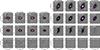 |
Fig. B.1. Surface brightness fit on the hosts of SNe 2010mc (left) and 2024hpj (right). For each band, the data, model, and residuals are shown. For SN 2024hpj, separate models for the exponential disc (second row) and spiral arms (third row) are shown. |
To apply a uniform treatment to all hosts, we decided on a simple model composed of an exponential star formation history (SFH, Carnall et al. 2018) and a Calzetti dust extinction law (Calzetti et al. 1994). The redshift was assumed to be the same as the one measured on the SNe. In total, we had five free parameters: the time since the beginning of the star-formation (Ageexp) and its timescale (τexp), the dust extinction in V-band magnitudes (AV), the metallicity relative to the solar value (Zexp/Z⊙), and integrated formed stellar mass across time log10(Mexp/M⊙). To quantify whether the hosts are star-forming or quiescent, we compare them with the star-formation main sequence (SFMS) obtained by Boselli et al. (2023) for a sample of H I-normal galaxies in the Virgo cluster spanning stellar masses within 107 < M* < 1011. The SFMS best fitting parameters are a slope of 0.92 ± 0.02, an intercept of −1.57 ± 0.53 computed at the reference mass of 108.451, and an intrinsic scatter of 0.42 dex. The SED fits are shown for each host galaxy in Fig. B.2.
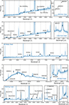 |
Fig. B.2. SED fit of the host galaxies of (from top to bottom) SNe 2010mc, LSQ13zm, 2016bdu, 2018cnf, and 2024hpj. |
In the following, we summarise the main results for each host galaxy:
2010mc host: we used the Pan-STARRS g, r, i, z flux densities measured with the surface brightness fitting and upper limits for the 2MASS J, H, K. The host appears to be a 108.15 M⊙ dwarf galaxy with a very low dust content (AV < 0.81 at the 95th percentile). The galaxy sits on the upper part of the main sequence with a log10(SFR)SED − log10(SFR)MS = 0.49, hence being a normal star-forming galaxy.
LSQ13zm host: we used the GALEX FUV and NUV, SDSS u, g, r, i, z, and WISE W1 flux densities available from NED. The host appears to be a 108.14 M⊙ dwarf galaxy with a high dust content ( at the 95th percentile). The galaxy sits well above the main sequence with a log10(SFR)SED − log10(SFR)MS = 1.29 (∼ × 3 the intrinsic scatter), consistent with the galaxy experiencing a starbursting phase.
2016bdu host: we used the SDSS u, g, r, i, z flux densities available from NED. The host appears to be a very low-mass 105.75 M⊙ dwarf galaxy with a low dust content (AV < 0.41 at the 95th percentile). The galaxy sits well above the main sequence with a log10(SFR)SED − log10(SFR)MS = 1.26 (∼ × 3 the intrinsic scatter), consistent with the galaxy experiencing a starbursting phase.
2018cnf host: we used the Johnson B, 2MASS J, H, K, and WISE W1, W2, W3, W4 flux densities available from NED. The host is the most massive galaxy on which we performed the fit, with a mass of 1010.19 M⊙. The metallicity is unconstrained, given the available photometry. The galaxy sits slightly below the main sequence with a log10(SFR)SED − log10(SFR)MS = −0.12. Nevertheless, given the intrinsic scatter of 0.42 dex, the host of SN 2018cnf is consistent with being a main sequence galaxy.
2024hpj host: we used the GALEX FUV and NUV and WISE W1, W2, W3 flux densities available from NED and the Pan-STARRS g, r, i, z flux densities measured with the surface brightness fitting. The host appears to be a 107.47 M⊙ dwarf galaxy with a very low dust content (AV = 0.10 ± 0.01), while the τexp in unconstrained. The posteriors of the metallicity seem to suggest very high values, with Zexp/Z⊙ > 1. The galaxy sits well above the main sequence with a log10(SFR)SED − log10(SFR)MS = 1.99 (∼ × 5 the intrinsic scatter), consistent with the galaxy experiencing a strong starbursting phase.
2019mry host: we used DEcam g, r, i, z and WISE W1, W2, W3, W4 flux densities available from the Legacy Survey (Dey et al. 2019) DR10 tractor catalogues. The host appears to be a 107.02 M⊙ dwarf galaxy with a very low dust content AV < 0.12 and a weakly constrained metallicity Zexp/Z⊙ < 1.32 (at the 95th percentile). The τexp in unconstrained. The galaxy sits well above the main sequence with a log10(SFR)SED − log10(SFR)MS = 0.62 (∼ × 1.5 the intrinsic scatter) being consistent with the galaxy experiencing a mild starbursting phase.
2023vbg host: we used the SDSS u, g, r, i, z and WISE W1, W2, W3, W4 flux densities available from NED. The host appear to be a 107.57 M⊙ dwarf galaxy with a very low dust content and subsolar metallicity AV < 0.10 and Zexp/Z⊙ < 1.02 (at the 95th percentile). The τexp in unconstrained. The galaxy sits well above the main sequence with a log10(SFR)SED − log10(SFR)MS = 0.95 (∼ × 2 the intrinsic scatter) being consistent with the galaxy experiencing a starbursting phase.
 |
Fig. B.3. Finding charts for the SNe in the sample. Each finding chart is a 2.33′×2.33′ cutout of a r band image from SkyView. In each image, a red cross marks the SN position. |
All Tables
All Figures
|
Fig. 1. Light curve and spectra of SN 2009ip. Left: Annotated R light curve showing the first outburst that marked the discovery of the transient in 2009, repeated outbursts during 2010 and 2011, and the main event in 2012. The inset zooms in on the latter, highlighting the presence of Events A and B. Different colours indicate the various light curve phases. Adapted from Pastorello et al. (2013). Data from Maza et al. (2009), Smith et al. (2010), Foley et al. (2011), Mauerhan et al. (2013), Fraser et al. (2013), Pastorello et al. (2013), Prieto et al. (2013), Margutti et al. (2014). Right: Selected spectra of SN 2009ip for key light curve phases (first discovery, repeated outbursts, Event A, and Event B). Numbers next to the spectra are computed from the epoch of first discovery. Data from Pastorello et al. (2013), Fraser et al. (2013). |
| In the text | |
|
Fig. 2. Finding chart for SN 2024hpj, observed on 27 May 2024 with NOT/ALFOSC in the g, r, and i bands. |
| In the text | |
|
Fig. 3. Apparent light curve of SN 2024hpj in the u, g, r, i, z, J, H, K, cyan, orange, w, and y bands. A rigid shift is applied for better visualisation. Top: Complete light curve covering the last ∼3 years. Bottom: Zoom-in on the Event A+B light curve. Dashed grey lines indicate the peaks of Events A and B, while grey arrows and open symbols indicate upper limits. Phases are calculated with respect to the epoch of the Event B maximum (MJD 60455). |
| In the text | |
|
Fig. 4. Spectral evolution of SN 2024hpj, with all spectra corrected for redshift and reddening. Numbers next to each spectrum indicate the rest-frame phase since the Event B maximum in the g band. Dotted lines indicate the position of major emission lines. |
| In the text | |
|
Fig. 5. Pseudo-bolometric light curve of SN 2024hpj, constructed by integrating the u to K bands. The expected theoretical decay rate due to 56Co is also shown. |
| In the text | |
|
Fig. 6. Fit of the peak (dotted blue line) and decline (dashed cyan line) of the multiband (g, r, i and orange) and pseudo-bolometric light curves. The secondary bump is excluded from the fit (see text). |
| In the text | |
|
Fig. 7. Residuals of the multiwavelength (upper panel) and bolometric (bottom panel) light curves after subtracting the peak and decline fits. Magnitudes are shifted for better visualisation. The dashed lines indicate the mean value of the residuals for each band. |
| In the text | |
|
Fig. 8. Evolution of Hα and Hβ during the first month after discovery. Left: Evolution of Hα in velocity space. Centre: Evolution of Hβ in velocity space. Numbers indicate the phase from the peak. Right: Flux ratios of |
| In the text | |
|
Fig. 9. Temperature, radius, and luminosity from the blackbody (BB) fit to the spectra. There is a clear decline during the first ∼60 days, while the data show a highly variable trend, likely indicating that the assumption of a BB is no longer valid. |
| In the text | |
|
Fig. 10. Expansion velocity measured from the minimum of the broad P-Cygni for Hα, He Iλ5876, and Fe IIλ5169, together with the corresponding power-law fits (black, red, and blue lines, respectively). A similar double trend is seen for Hα before and after phase +30 days, while He I follows a power-law decline, although, it is contaminated by Na I D, especially at late phases. The Fe II line also shows a power-law decline, albeit with some scatter, possibly due to the difficult identification. |
| In the text | |
|
Fig. 11. Light curves of objects observed in our sample. Each SN is shown in the best-sampled broadband light curve. Comparisons with SN 2024hpj and, when available, SN 2009ip, are also included. Phases are calculated from the Event B peak. The luminosity at this peak and the subsequent decline rate are very similar, whereas there is some variation in the duration and brightness of Event A. Arrows and open symbols indicate upper limits. |
| In the text | |
|
Fig. 12. Spectral evolution of objects observed in our sample. All spectra are redshift- and reddening-corrected and rescaled for better visualisation. Numbers close to the spectra indicate the rest-frame phase from the Event B peak. |
| In the text | |
|
Fig. 13. Individual pseudo-bolometric light curve of SN 2024hpj (mauve points) compared with the sample SNe. All light curves are matched at the Event B peak (for SN 2022mop, only the 2024–2025 period is shown). Labels indicate the bands used to build the light curve (see text). Four groups are discernible: rise and/or decay time and peak luminosity similar to SN 2024hpj (group 1); more luminous and/or faster declining than SN 2024hpj (group 2); slower declining than SN 2024hpj (group 3); and exhibiting a plateau (group 4). |
| In the text | |
|
Fig. 14. Magnitude at the Event B peak as a function of the magnitude at the Event A peak. Measurements were performed in the r and R bands when available. For SNe not covered during Event A in r (SNe 2025csc, 2022ytx, and 2019mry), we performed the measurements in the orange band for SNe 2025csc and 2022ytx, and in the I band for SN 2019mry. Colours are the same as in Fig. 13. Error bars are present but often smaller than the data points. |
| In the text | |
|
Fig. 15. Spectral comparison of SN 2024hpj with selected SNe from the sample. Left: Comparison around the Event B peak. Right: Comparison approximately 100 days after the Event B peak. Numbers in parentheses indicate the group based on the light curve (see text). Phases from the Event B maximum are also reported. All spectra are redshift- and reddening-corrected. |
| In the text | |
|
Fig. 16. Distribution of host morphology as a function of the t parameter and SN distance from the host-galaxy centre for SNe in the volume- and time-limited sample (within 100 Mpc, discovered after 2009). |
| In the text | |
|
Fig. B.1. Surface brightness fit on the hosts of SNe 2010mc (left) and 2024hpj (right). For each band, the data, model, and residuals are shown. For SN 2024hpj, separate models for the exponential disc (second row) and spiral arms (third row) are shown. |
| In the text | |
|
Fig. B.2. SED fit of the host galaxies of (from top to bottom) SNe 2010mc, LSQ13zm, 2016bdu, 2018cnf, and 2024hpj. |
| In the text | |
|
Fig. B.3. Finding charts for the SNe in the sample. Each finding chart is a 2.33′×2.33′ cutout of a r band image from SkyView. In each image, a red cross marks the SN position. |
| In the text | |
Current usage metrics show cumulative count of Article Views (full-text article views including HTML views, PDF and ePub downloads, according to the available data) and Abstracts Views on Vision4Press platform.
Data correspond to usage on the plateform after 2015. The current usage metrics is available 48-96 hours after online publication and is updated daily on week days.
Initial download of the metrics may take a while.