| Issue |
A&A
Volume 707, March 2026
|
|
|---|---|---|
| Article Number | A156 | |
| Number of page(s) | 18 | |
| Section | Extragalactic astronomy | |
| DOI | https://doi.org/10.1051/0004-6361/202556973 | |
| Published online | 03 March 2026 | |
Broad iron line as a relativistic reflection from warm corona in AGNs
1
Nicolaus Copernicus Astronomical Center, Polish Academy of Sciences Bartycka 18 PL-00-716 Warszawa, Poland
2
ESIA, Observatoire de Paris, PSL Research University, CNRS, Sorbonne Universités, UPMC Univ. Paris 06, Univ. Paris Diderot, Sorbonne Paris Cité 5 place Jules Janssen F-92195 Meudon, France
3
Research Center for Computational Physics and Data Processing, Institute of Physics, Silesian University in Opava Bezručovo nám. 13 746 01 Opava, Czech Republic
★ Corresponding author: This email address is being protected from spambots. You need JavaScript enabled to view it.
Received:
25
August
2025
Accepted:
19
January
2026
Abstract
Context. We present that the broad feature usually observed in X-ray spectra at around 6.4 keV can be explained by ray-traced emission from the two-slab system containing a dissipative, warm corona on the top of an accretion disk in an active galactic nucleus (AGN). Such an accretion flow is externally illuminated by X-ray radiation from a lamp located above a central supermassive black hole (SMBH). Thermal lines from highly ionized iron ions (FeXXV and FeXXVI) caused by both internal heating and reflection from the warm corona, can be integrated into the observed broad line profile due to the close vicinity to the SMBH.
Aims. We investigate the dependence of the total broad line profile on the variations in black hole spin parameter, viewing angle, lamp height, and dissipation factor. Our results introduce a new method to probe properties of warm corona using high-resolution spectroscopic measurements with current XRISM and future NewATHENA X-ray missions.
Methods. We use photoionization code TITAN to compute local ion population and emission line profiles, and ray-tracing code GYOTO to include relativistic effects on the outgoing X-ray spectrum.
Results. In our models, the temperature of the inner atmosphere covering the disk can reach values of 107 − 108 K due to warm corona dissipation and external illumination, which is adequate for generating highly ionized iron lines. These lines can undergo significant gravitational redshift near the black hole, leading to a prominent spectral feature centered around 6.4 keV.
Conclusions. For all computed models, relativistic corrections shift highly ionized iron lines to the 6.4 keV region, usually attributed to fluorescent emission from the illuminated skin of an accretion disk. Hence, for a warm corona that covers the inner disk regions, the resulting theoretical line profile under strong gravity is a sum of different iron line transitions, with highly ionized iron contributing the most to the total line profile observed in an AGN.
Key words: accretion / accretion disks / black hole physics / radiative transfer / relativistic processes
© The Authors 2026
 Open Access article, published by EDP Sciences, under the terms of the Creative Commons Attribution License (https://creativecommons.org/licenses/by/4.0), which permits unrestricted use, distribution, and reproduction in any medium, provided the original work is properly cited.
This article is published in open access under the Subscribe to Open model. This email address is being protected from spambots. You need JavaScript enabled to view it. to support open access publication.
1. Introduction
Active galactic nuclei (AGNs) are one of the most prominent X-ray sources. The existence of a reflection component with Fe Kα fluorescent emission was first discussed by Lightman & White (1988). The features were initially reported by Pounds et al. (1990), which implies a cold accretion disk with a temperature around 105 K (Guilbert & Rees 1988) that emits the fluorescent iron line (FeI-FeXVI, Kallman & McCray 1982) caused by a reflection from neutral material. With an improved resolution of XMM-Newton and Chandra X-ray telescopes, a broad iron line was reported with a narrow core (e.g., Yaqoob et al. 1995; Nandra et al. 1997; Reeves 1990; Guainazzi et al. 2006), suggesting a relativistic broadened feature originating from the inner accretion disk, while the narrow core was emitted from a distant region (see Fabian et al. 2000; Nandra 2006; Nandra et al. 2007; Andonie et al. 2022). The broadening of the fluorescent Fe Kα line generated very close to the supermassive black hole (SMBH) is subject to relativistic effects like rotational broadening, relativistic boosting, and gravitational redshift, which generates the characteristic double-peaked, disk-like, emission line (Laor 1991). Thus, the overall shape of the line profile depends on the spin of the SMBH and the observer’s viewing angle (Fabian et al. 2000).
An accepted scenario is that the observed iron line is created due to the reflection of external hard X-rays from the inner regions of an accretion disk (Fabian et al. 1989; George & Fabian 1991). Strong illumination supports the formation of the so-called “ionized skin” on the top of an accretion disk (Ross & Fabian 1993; Nayakshin et al. 2000; Madej & Różańska 2000; Ballantyne et al. 2001; Różańska et al. 2002). Models of ionized skin, such as relxill (García et al. 2014, and references therein) are commonly used to interpret X-ray reflected spectra of AGNs.
Nevertheless, ionized skin was shown to be relatively optically thick (Różańska et al. 1999). However, recent X-ray data show the existence of a soft X-ray excess in the majority of AGNs (e.g., Boissay et al. 2016; Gliozzi & Williams 2020). The origin of such excess is still under debate, but recent studies strongly favor the presence of a warm corona, i.e., a high-temperature (kBT ∼ 2 keV, where kB is the Boltzmann constant) structure close to the SMBH. A warm skin on top of the accretion disk (Petrucci et al. 2013) is an important part of the so-called two-corona model (Petrucci et al. 2018): i.e., a fully ionized hot corona inner structure as an origin of observed power-law emission, and a warm corona as an origin of soft X-ray excess. The final spectrum of such a model consists of soft excess together with the power law, and it was successfully used for the interpretation of high-resolution X-ray data of many AGNs (Done et al. 2012; Petrucci et al. 2018; Ballantyne et al. 2024; Palit et al. 2024). It was analytically shown by Różańska et al. (2015) that to produce a warm optically thick layer, covering a cold accretion disk, the inclusion of an internal dissipation in the warm corona is required, in addition to radiation and strong Compton cooling. This suggests that the emissivity profile deviates from the prediction of a standard disk atmosphere. Furthermore, radiation magneto-hydrodynamic simulations of the accretion disk around an SMBH indicated the existence of a dissipative warm or hot slab as an upper zone of the accretion disk atmosphere (e.g., Jiang et al. 2019b, and references therein).
As the temperature in the warm corona is high, iron atoms are likely to be highly ionized. The warm corona temperatures, of the order of ∼2 keV, are suitable for the emission of Fe Kα from highly ionized species such as FeXXV and FeXXVI (Bianchi & Matt 2002). It is worth mentioning that from a theoretical point of view, if the Kα transition originates from the high-ionization states of iron, such as FeXVII–FeXXIV, the line photons undergo resonant Auger destruction, significantly reducing their emission intensity (Liedahl 2005). We also expect the warm corona to be very close to the SMBH, which subjects the FeXXV and FeXXVI iron lines to strong gravitational effects. A broad emission feature, likely from highly ionized iron ions, was already reported by Reeves et al. (2001) and Pounds et al. (2001). If the highly ionized Fe Kα lines are generated very close to the SMBH, then we also expect them to get gravitationally redshifted moving away from their core emission region, broadened due to rotation, and Doppler boosting. Hence, the broad line observed around the 6.4 keV region may be composed of many transitions on highly ionized iron ions.
In this work, we show the effects of strong gravity subjected to the highly ionized Fe Kα profiles produced in the warm corona. To do so, we consider the two-corona model schematically presented in Fig. 1. The radiation from a hot corona illuminates a two-zone structure: an accretion disk that is surrounded by a dissipative, Compton-cooled warm corona. In addition, a warm atmosphere at the top of an accretion disk is radially stratified. Due to its dissipative nature, the inner regions of the disk atmosphere may reach temperatures characteristic of a warm corona at a large optical depth (Różańska et al. 2015; Petrucci et al. 2020). At such high temperatures, the spectrum is dominated by the emission of highly ionized Fe Kα ions (FeXXV, FeXXVI) (Ballantyne 2020). Contrary to the ionized skin that is only heated by external illumination, the warm corona is additionally heated by an internal mechanical process, which ensures its high temperature from the outset. The highly ionized Fe Kα lines produced in the warm corona close to the SMBH are relativistically redshifted, broadened due to fast rotation of the disk, and relativistically boosted, appearing as a broad Fe Kα structure. To model highly ionized iron line profiles in the close vicinity of an SMBH, we used a combination of the photoionization code TITAN (Dumont et al. 2000, 2003) and the publicly available ray-tracing code GYOTO1 (Vincent et al. 2011). The radiative transfer code TITAN produces angle-dependent intensities with all relevant iron lines, illuminated in the warm corona on top of the cold disk. Those intensities act as the input for GYOTO to compute the final ray-traced spectrum seen by the distant observer. This form of modeling enables us to include relativistic effects in the computed spectrum for different viewing angles and black hole spins. The GYOTO code was already used to ray trace the reflected spectra from X-ray binaries (Vincent et al. 2016). In addition to the proper treatment of all spectral effects, like many other convolution ray-tracing models for X-ray data analysis, GYOTO also produces images at the assumed energy range, which we present here.
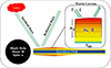 |
Fig. 1. A schematic diagram of our model’s setup. A hot corona, as in lamppost geometry, is located at height h above the SMBH of mass M and spin a. The warm corona is positioned on top of an accretion disk. The incident flux coming from the hot corona is reprocessed in the warm corona, which is then detected by the observer. The rin and rout are the integration limits for our model. We compute the vertical structure using TITAN with the input parameters depicted in the warm corona panel; Γ – photon index, ξ – ionization parameter, NH – column density, nH – gas number density, Q – internal heating, and TBB – the temperate of blackbody radiation from an underlying disk. |
The goal of this paper is to follow the same scheme of computations as in the reXcor model of Ballantyne et al. (2024), but with the use of different computational codes. Nevertheless, the global disk solutions for its radial structure remain the same. Since our radiative transfer code TITAN contains a rich set of iron transitions and angle-dependent emission, we can deeply investigate the region of the iron line complex in the reflected spectrum. In this paper, the Compton scattering is included in the total energy balance, and therefore, the gas temperature is determined correctly. We decided not to include the broadening of the lines due to Compton scattering to first study purely relativistic broadening. The model description on how to combine TITAN and GYOTO computations with their assumptions is discussed in Section 2. The results are presented in Section 3. Finally, Section 4 is dedicated to discussion and conclusions.
2. Model description
We calculate the observed emission from the inner part of an accretion disk atmosphere in plane-parallel geometry. A schematic representation of our model is shown in Fig. 1. We assume a dissipative warm corona on top of a geometrically thin and optically thick accretion disk. We adopt a lamppost geometry, where the disk is illuminated by a source placed at a height h above the black hole, along the spin axis (e.g., Matt et al. 1991; Martocchia & Matt 1996; Dauser et al. 2013). The lamp represents a hot corona with power-law emission, which illuminates the warm optically thick corona in the direction normal to the surface. The effect of gravitational light bending of the illuminated radiation is schematically taken into account in Eq. (5) below. We note that the lamp approximation holds, given that the height of the lamp is not too small, where the light bending is extreme.
In our calculation of the observable emission, we chose a region very close to the SMBH where the relativistic effects are dominant, and the relatively high temperature of the warm corona can produce highly ionized Fe Kα ions. For the assumed black hole mass – M, dimensionless spin – a, and disk accretion rate – λ, we calculate radially dependent parameters of gas and radiation defined on the top of the atmosphere given in Sect. 2.1.
In the next step, for each radius considered, these parameters are input for the radiative transfer code TITAN, which calculates the emergent spectrum from an ionized, illuminated, and dissipated atmosphere, i.e., an optically thick warm corona with a defined optical thickness τWC. For this paper, we are interested in the iron line spectral region; therefore, we treat Compton scattering only in the expression of cooling and heating functions as described in Sect. 2.2 below. The full code, which solves photoionization with Compton scattering on the microscopic level, is under construction by our team, and its results will be presented in our future work.
Finally, after collecting the angle and radial dependent intensity field for a given set of global disk parameters, as M, a, and λ, we use GYOTO to calculate the image and spectrum seen by a distant observer (see Sect. 2.3). We analyze the emergent spectra as a function of black hole spin, viewing angle, and disk matter structure for the model setup given in Sect. 2.4.
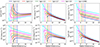 |
Fig. 2. Radial distribution of global model parameters that are inputs for TITAN code. The colors represent different spin values given in the top box. The subplots are as follows: top left panel: gas number density (Eq. (1)), top middle panel: dissipation flux (Eq. (2)), top right panel: X-ray flux from a hot corona (Eq. (5)), bottom left panel: ionization parameter (Eq. (9)), bottom middle panel: internal heating of the warm corona (Eq. (10)), and bottom right: accretion disk temperature TBB (Eq. (11)). The vertical dashed lines mark the radius at which the output temperature structure from TITAN reaches the maximum, see Fig. 3 and text for details. |
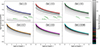 |
Fig. 3. Temperature dependence on the optical depth for various spin values given in the boxes. The gray gradient of lines represents the matter structure calculated at different radii, with the darkest line at rin, and the lightest line at rout. The colored lines show the simulation with maximum temperature, which is consistent with the dashed line in Fig. 2. The corresponding radial point where the temperature drop is observed is labeled and marked in green text. The parameters other than spin are chosen to be canonical values from Table 2. As this is the temperature structure, it is independent of the viewing angle. |
2.1. Radial stratification
For the radial stratification of the warm corona, we follow the same prescription as in Xiang et al. (2022); hence, in the following section, we reiterate the formalisms they described. In our approach, the disk is radially stratified into 20 uniformly spaced zones from rin = rISCO + 1 rg to rout = 25 rg (we assume that the maximum flux comes from within this region and the effects of strong gravity is minor beyond this radii) (see Appendix B). Here, ISCO is defined as the innermost stable circular orbit of a prograde accretion disk, and rg = GM/c2 is the gravitational radius, M – mass of the black hole, G and c being the gravitational constant and the speed of light in vacuum, respectively. Note that 1 rg is added to avoid the nonphysical increase of the disk number density in Eq. (1) (Xiang et al. 2022).
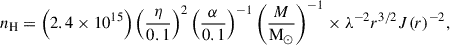
To compute the radially stratified gas number density of the warm corona, we first consider the mid-plane density from Svensson & Zdziarski (1994) and assume that the density falls by 103 to the surface (e.g., Jiang et al. 2019a). Hence, the gas number density in cm−3, for a disk atmosphere, is given by
 (1)
(1)
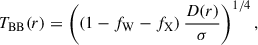
where r is the radial distance in units of rg, the accretion rate λ = Lbol/LEdd where Lbol is the bolometric luminosity and LEdd = 4πGMmpc/σT is the Eddington luminosity (with mp being mass of proton and σT as the Thompson cross section), η is the accretion efficiency, α is the viscosity parameter, and J(r) = 1 − (rISCO/r)1/2 is the stress-free inner boundary condition in a standard thin disk model (Shakura & Sunyaev 1973). The radial dependence of the gas number density is shown in the top left panel of Fig. 2.
The total energy flux D(r) in erg cm−2 s−1, produced by each side of a standard accretion disk due to dissipation, is given by
 (2)
(2)
This dissipative flux is further divided into three contributing fractions: the illuminating X-ray flux fraction fX determines the total X-ray luminosity of the hot corona, i.e., lamp; the dissipative flux fraction fW determines the dissipation due to internal heating of the warm corona; and (1 − fX − fW) of D(r) determines the accretion disk flux that enters the atmosphere from below in the form of blackbody radiation with TBB temperature.
For two-corona geometry, we assume a power-law spectrum emitted by the hot corona (lamp) with the photon index Γ following the relation E−Γ ∝ photon flux. This hot corona within a critical radius rc emits the X-ray luminosity in erg s−2
 (3)
(3)
where dSdisk is the area of the proper disk element adapted from Vincent et al. (2016) that depends on the spin and radius of the black hole as
 (4)
(4)
The critical radius of the hot corona rc is assumed to be at 10 rg, which considers a highly compact corona consistent with observations (e.g., Miniutti & Fabian 2004; Reis & Miller 2013). Following Xiang et al. (2022), we assume that the regions above rc do not contribute to the hot corona, because the dissipation factor falls rapidly beyond 10 rg having negligible effects on the hard X-ray spectrum.
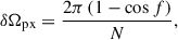
Given that the X-ray luminosity originates from the lamppost source, the incident X-ray flux reaching the disk atmosphere is subjected to gravitational light bending and hence depends on the height of the lamp h and the dimensionless spin parameter a (e.g., Miniutti & Fabian 2004; Fukumura & Kazanas 2007; Dauser et al. 2013). The radially stratified X-ray flux in erg cm−2 s−1 is defined as (Ballantyne 2017)
 (5)
(5)
where F(r, h) is given by the fitting formula proposed by Fukumura & Kazanas (2007) for the illumination pattern of the disk, glp is the ratio of the photon frequency on the disk to that at the X-ray source (Dauser et al. 2013),
 (6)
(6)
and z(M) is used to convert the area into physical units (Ballantyne 2017)
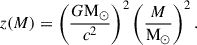 (7)
(7)
Finally, the integrated total flux corresponds to LX via the normalization factor given by
 (8)
(8)
The X-ray flux and the gas number density can further be used to define the ionization parameter ξ(r) in erg cm s−1 as
 (9)
(9)
The radial dependence of the X-ray flux and the ionization parameter is depicted in Fig. 2.
The internal heating Q(r) in units of erg cm2 s−1 that occurs in the disk atmosphere is uniformly distributed throughout the vertical structure of the warm corona with the given optical depth τWC, and it is defined by the dissipative flux fraction fW as
 (10)
(10)
Finally, the remaining dissipative energy contributes to the warm corona as a back-illumination from the accretion disk. It enters an atmosphere from below and follows the blackbody shape of the spectrum with the corresponding temperature TBB(r) in K given by
 (11)
(11)
where σ is the Stefan-Boltzmann constant. The above radially stratified parameters are further used as input parameters to the photoionization code TITAN, described in the following section.
2.2. Radiative transfer with TITAN
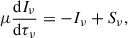
The radiation emitted from the atmosphere covering the underlying accretion disk is computed using the photoionization code TITAN, specifically with its most advanced version described by Dumont et al. (2003). With the given input parameters, TITAN solves the radiative transfer through the slab of gas
 (12)
(12)
where μ is the cosine of the angle between normal and light ray, Iν is the specific intensity at the angle μ, Sν is the source function, and τν is the optical depth. The slab is divided into discrete horizontal layers, and the transfer of radiation is calculated using the accelerated lambda iteration method under non-local thermodynamic equilibrium (nLTE) conditions (Dumont et al. 2003). It assumes a two-stream approximation where two intensities are from top to bottom of the disk atmosphere as the inward flux and from bottom to top as the backward flux.
Within each layer, the physical state of the gas (ion abundances, temperature, and level population) is computed by solving a local balance between ionization and recombination ions, excitations and de-excitations, local energy balance (radiative and mechanical heating is balanced by radiative cooling), and total energy balance (equality of total inward and outward energy flows) (Dumont et al. 2000). All relevant radiative processes, such as: free-free processes, i.e., bremsstrahlung; Compton heating and cooling; bound-free processes, i.e., photoionization and recombination; and finally bound-bound processes, such as line heating and cooling, are taken into account.
The number of ionic transitions taken into account is 4141 in the energy range between 0.01 eV and 25 keV. The ten most abundant elements are taken into account: H, He, C, N, O, Ne, Mg, Si, S, and Fe with solar abundances. In general, it is possible to change the gas content, but due to the model complexity, we keep them constant at the values provided by Grevesse & Anders (1989). There are two more parameters, which are inputs to TITAN’s models, but we keep them constant for better visualization of our results. Those parameters are the total column density NH, and the photon index Γ of the power-law shape of incident hard X-rays (see Secy. 2.4 for their values).
Currently, TITAN has two modes of operation, with constant density and constant total pressure. The constant density mode assumes a constant density for all layers of the slab (disk atmosphere), which are stratified against temperature. The constant pressure assumes a constant total (i.e., gas + radiation) pressure throughout the structure, varying both density and temperature. For this paper, we have prescribed a constant density, where at each radius the density number nH(r) is given by Eq. (1). The rest of the input parameters required by the TITAN code are the ionization parameter ξ(r), the internal heating of the warm corona Q(r), and the blackbody temperature TBB(r), and they change with radius according to radially stratified Eqs. (9), (10), and (11), respectively.
TITAN computes the output intensity spectra for six fixed angles i, listed in Table 1, defined as an inclination between the normal to the slab and the line of sight towards an observer. In addition, Table 1 displays the cosine of these angles in column 2, the solid angles being roots of the Gauss-Legendre quadrature used for numerical integration of the total energy flux. These angle-dependent intensities are further used as input parameters for the ray-tracing code GYOTO. Note that the above angles are used only to represent the angular dependence of local intensities emitted from the slab, and the proper viewing angle of the total system is an output parameter of GYOTO during ray-tracing computations.
Angles prescribed in TITAN.
2.3. Relativistic ray-tracing with GYOTO
GYOTO is a relativistic ray-tracing code that computes null geodesics for photons using the 3+1 formalism, in which a 4D spacetime is foliated into 3D spatial hypersurfaces and a 1D timelike direction (see Gourgoulhon 2007; Alcubierre 2008; Baumgarte & Shapiro 2010). It assumes a square screen with a total number of pixels N = n × n, where n is a 1D pixel number. Hence, a total of N photon paths are traced back to the source – one from each pixel on the screen (Luminet 1979).
To compute the ray-traced spectrum with GYOTO, we used the directional disk option of the code, which was previously tested by Vincent et al. (2016) in the case of an illuminated accretion disk around an SMBH. This model allows us to include the relativistic effects caused by a central black hole on the intensity spectrum emitted locally from a flat equatorial disk. The spectral input is organized as intensity varying with both viewing angle and radial distance from the black hole, while the disk is cylindrically symmetric and emits only from its surface. The model is constructed under the assumption of Kerr geometry, assuming Boyer-Lindquist coordinates; thus, both mass M and spin a are input parameters.
The resulting intensities from TITAN are treated as locally emitted intensities Iνem in erg cm−2 s−1 Hz−1 sr−1, while the observed intensities measured by a distant observer are given by
 (13)
(13)
where g = νobs/νem is the redshift factor, with νobs and νem as the observed and emitted photon frequency, respectively. The computed observed specific intensity is then further used to calculate the observed monochromatic flux in erg cm−2 s−1 Hz−1:
 (14)
(14)
subtended by the solid angle dΩobs, where θobs is the angle between the angle normal to the screen and the angle normal to the accretion disk, which corresponds to the viewing angle. As customary in ray-tracing calculations, the observed solid angle equals the angle that subtends the field of view used on the screen.
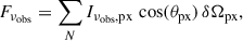
Of the total number of N pixels on the screen, each pixel (assumed to be a point-like object) corresponds to a specific direction in the sky. The object on the screen is defined by the field of view, the pixels that cover the field of view, and the spectral property used, such as the channels and their corresponding wavelengths (or energies) (Vincent et al. 2011). Each pixel covers a small field of view δΩpx, which is defined as the total field of view divided by the total number of pixels
 (15)
(15)
where f is the angle of the normal to the screen and the most distant incident angle of the photons on the screen. Using Eq. (14), the total observed flux can therefore be defined by
 (16)
(16)
where θpx is the angle between the normal to the screen and the direction of incidence corresponding to this pixel. As the screen is not a point source, θpx is not identical to θobs. At large observer (screen)–source distances, the angle subtended by a pixel, θpx, may differ only slightly from the viewing angle θobs; however, at shorter distances, this deviation can become significant. At each frequency, the flux at every pixel is computed on the basis of the radial distance and viewing angle corresponding to that pixel, resulting in a 2D image. Integrating over this image gives the total flux at that frequency. Repeating this process across all frequencies yields the relativistically corrected spectrum. Detailed computations of the frequency-dependent flux with more models can be found in Vincent et al. (2011). Finally, the observed flux is transformed into frequency-dependent luminosity using
 (17)
(17)
where Lν is defined in erg s−1 Hz−1 and D is the distance of the source from the observer.
2.4. Setup of parameters
In this paper, we pay special attention to the spectral shape of the iron line modified by gravitational effects from the SMBH. Therefore, we test only one case of black hole mass M = 108 M⊙ and accretion rate λ = 0.1, concentrating solely on the dependence of black hole spin – a, viewing angle – θobs, fraction of X-ray illuminating flux from the lamp – fX, fraction of dissipation in warm corona – fW, and the height of the lamp – h. The rest of the global disk parameters are taken to be fixed at: η = 0.1 and α = 0.1. We are aware that the accretion efficiency depends on the SMBH spin. But since we are not solving any dynamical equations of an accretion flow and this value is only needed to define the accretion rate and therefore the total energy dissipated at the given radius, we keep it constant for all models considered (also prescribed in Xiang et al. 2022).
The variation of the model parameters that affect the shape of the outgoing iron line profile is depicted in Table 2. We show our parameter space in the table with the first column depicting the variable parameter, the second column showing values of the computed grid, and the last column showing the canonical parameters, i.e., constant values for each parameter, while others are varied. The canonical values allow us to isolate and study the effect of each parameter individually. Spin dependence occurs in the inner boundary condition J(r), due to the different rISCO values. Since the accretion disk is modeled as geometrically thin and optically thick, we assume a constant optical depth of the top layer of the warm corona at a value of τWC = 5 throughout the entire radial structure. We are aware that some hard X-ray photons are getting thermalized at larger optical depths, but since our conditions change with radius, we keep this amount at a moderate value and uniform throughout all radially stratified zones. As the incident photon spectrum follows a power-law distribution, we fix the photon index to Γ = 2 at all radial points. There is a possibility to change the elemental abundances in TITAN code, but in this paper, we keep them fixed to the solar values.
List of model parameters.
Computations by TITAN result in angle-dependent intensities at each radial point considered. These angles and radial-dependent intensities are then used as the input spectra into the GYOTO code that integrates them over the disk surface, considering all relativistic effects in the Kerr geometry assuming Boyer-Lindquist coordinates. In principle, we can study the final outgoing spectrum for a large grid of parameter space, but for this paper, we consider values given in Table 2. The observer’s viewing angle directly corresponds to θobs from Eq. (14), and the lowest value reflects a face-on projection, while the highest value provides an edge-on view of the source.
The field of view is set to 5 μas to study the inner region of the SMBH, and it is assumed that the observer is at a large distance of D = 16.9 Mpc, far enough to ensure flat spacetime. We kept the resolution of N = 801 × 801 pixels for our simulations, which is reasonable for image resolution in the X-ray domain.
GYOTO can also generate photons originating from the photon ring region, which are classified as higher-order photons due to the multiple orbits they complete around the compact object. However, this region was excluded from the analysis due to resolution limitations, and only first-order photons were considered. Although higher-order photons were neglected in our work, it was demonstrated by Falanga et al. (2021) that their contribution to the observable iron line profiles is minimal.
3. Results
Our results are strictly focused on the iron line profile originating from the innermost region of the SMBH. The correctness of our ray-tracing procedure is tested in the case of a single Gaussian line on a flat continuum in Appendix A. Although the luminosity level of a single line test is consistent with the AGN disk luminosity, to have a realistic scenario, we used the ray-tracing code GYOTO on the reflected spectra calculated by the TITAN code, which physically changes with radial distance from the SMBH. We present those results in the following sections.
3.1. Matter structure and local spectra
We used the photoionization code TITAN to generate the local emitted spectrum from the disk atmosphere. At each radially stratified point, TITAN computes the vertical structure, in which the Compton process is simplified, but ionization is computed more rigorously with a large database of atomic transitions. The radial evolution of the input parameters needed locally for TITAN code, as described in Section 2.1, is shown in Fig. 2. The gas number density is observed to initially fall and then rise with the increase in the radial distance from the SMBH, but in general the disk atmosphere is very dense, as expected in the case of accretion disks around SMBHs. The initial fall occurs due to the stress-free inner boundary condition. Hence, very close to rISCO, the gas number density can reach nonphysical values, due to which we start our simulations from rISCO + 1 rg.
The total energy flux D(r) decreases with the r−3 dependence, and is presented in the top middle panel of Fig. 2. It directly affects the other parameters, such as the X-ray power-law illumination flux FX(r) – top right panel, the internal heating parameter Q(r) – bottom middle panel, and back illumination Temperature TBB(r)– bottom right panel. Both Q(r) and the ionization parameter ξ(r) also exhibit inverse dependencies on the gas number density nH(r) – specifically, Q(r)∝nH(r)−1 and ξ(r)∝nH(r)−1 – which further suppresses their values. With these given input parameters of nH(r), Q(r), ξ(r), and TBB(r) in each of the 20 equally spaced radial zones between rISCO + 1rg and 25rg, we compute the vertical structure with TITAN radiative transfer code assuming at each radius constant photon index Γ and the warm corona optical depth τWC. During radiative transfer computations, we use the assumption of constant density throughout the vertical gas zones given in the optical depth of electron scattering τ.
One of the outputs generated by TITAN is the vertical matter structure with which we can study the temperature at each optical depth of an atmosphere. This temperature results from the solution of the energy equilibrium equation, where all cooling processes balance all heating processes, radiative plus mechanical. The dependence of the vertical temperature profiles for various spin values and at different radial points is depicted in Fig. 3. As we go vertically deeper into the layers, the optical depth increases and the temperature decreases. The temperature also decreases with the increase of the radius, depicted by the change in the gradient of lines, where the dark lines represent the innermost radii and the light gray lines represent the outer regions (see the sidebar of Fig. 3).
As the black hole spin increases, the disk’s temperature also increases. This occurs mainly because of the disk model we use, where the amount of energy released increases with spin. Spin affects the inner edge of the disk, and with higher spin, the value of J(r) increases. This causes D(r), the energy flux being given off, to increase as well. As a result, the disk gives off more energy overall, making it hotter.
We also detected a sudden fall in temperature for spin values of: 0, 0.3, and 0.5 at radii 21.385 rg, 24.298 rg, and 25.737 rg, respectively. This temperature drop may be caused by the change in the radiative heating or cooling mechanism operating in the gas. To investigate the origin of the above temperature drop, in Fig. 4 we plot the vertical heating and cooling profiles computed by the TITAN code for three consecutive radii: before the drop – top panel, during the drop – middle panel, and after the drop – bottom panel, for the spin case a = 0. All relevant processes taken into account are listed in the box above the panels. We see that in all cases, mechanical internal heating dominates throughout the atmosphere. Nevertheless, there is a difference between the structure of the radiative cooling, which starts to dominate as the optical depth increases. Deeper, at about τ = 3.5 net line cooling starts to outweigh Compton and bremsstrahlung cooling, causing the final temperature drop. In the lower panel, when the overall atmospheric temperature is lower, line cooling dominates all cooling processes throughout the entire thickness of the warm corona. The radial location of the temperature drop corresponding to higher spin shifts outward, implying that line cooling becomes dominant for higher spin at larger radii, i.e., larger than rout, outside our computational limit.
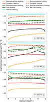 |
Fig. 4. Heating and cooling of the matter structure at equilibrium for spin 0 and mass 108 M⊙. The plots depict different points of the radial structure, left: 20.538, middle: 21.385, right: 22.231 rg. The solid lines depict heating and the dashed lines depict cooling. |
The initial parameterization of the input also produces a peak in the temperature profile within the grid domain of our radial structure. In Fig. 2, we mark with dashed lines the radial point where we see the highest temperature in our radial structure. Such a peak arises primarily due to the global model, and it aligns closely with the peak of the internal heating parameter D(r). This shows that even though roughly 40% of the dissipative flux is in the form of internal heating, the energy balance at equilibrium is dominated by the heating provided to the structure. Overall, the peak of the matter structure shifts inward with an increase in spin, suggesting that a higher spin value will have a hotter temperature structure near the ISCO. Since the back-illumination temperature is lower than that of the disk atmosphere, seed photons from the disk in the form of blackbody radiation contribute to the net cooling of the atmospheric layers.
The reflected spectrum produced by TITAN for different spins at an angle of 17.6° is illustrated in Fig. 5. The direct influence of temperature can be seen with the variation in the strength of the highly ionized Fe Kα lines. With an increase in spin, the temperature of the disk rises, which is apparent from the effect where the FeXXV ions get ionized to FeXXVI, increasing the strength of the line at 6.957 keV. Absorption features are also observed in the spectrum emitted locally from the disk. These arise due to the dissipation of energy within the disk and the presence of photons transmitted from its deeper layers.
 |
Fig. 5. Local spectra νFν versus photon energy E, from TITAN code, for different spin values at the i = 17.6°. The gray gradient of lines depicts outgoing spectra calculated at different radii, with the darkest line at rin, and the lightest line at rout. The colored lines show the simulation with maximum temperature, which is coherent with the dashed line in Fig. 2 and solid colored lines in Fig. 3. The parameters other than the spin and the viewing angle are set to be canonical values as depicted in Table 2. |
Note that in the case of a warm corona, illuminated photons from the hot corona are generally more energetic than warm gas on the top of the disk and mostly cause photoionization and excitation processes. This gives rise to the line emission, which may exceed the Compton cooling of the matter. On the other hand, soft photons from the disk are the major drivers for Compton up-scattering, i.e., Compton cooling, which we expect to be responsible for soft X-ray excess emission from the warm corona (Petrucci et al. 2018; Ballantyne et al. 2024; Palit et al. 2024). Furthermore, in a gas of relatively high density, bremsstrahlung cooling becomes dominant, which can provide stability to thermally unstable matter as studied by Adhikari (2019), Gronkiewicz et al. (2023). Despite these specific features, we see that under our assumptions, the warm atmosphere can be sustained, and locally the resonant iron Kα lines can be created and then subject to relativistic blurring.
3.2. Ray-traced spectrum
In the previous section, we demonstrated that, for the assumptions of the global disk model and with the assumed emitting surface, highly ionized Fe Kα lines can be created in the local spectrum of the warm and dissipative corona. This section discusses the output from GYOTO, where we include the relativistic effects in the emitted spectrum. We start with an illustration of the image produced by GYOTO at 6.4 keV in Sect. 3.2.1. Following a 2D integration of the image at each frequency, we obtain the relativistically corrected spectrum. Hence, in the following subsections, we show the dependence of the output spectrum on the spin of the SMBH, viewing angle, height of the lamp, and the dissipative flux distribution.
3.2.1. GYOTO image
For the given viewing angle and spatial resolution, the GYOTO code produces ray-traced images at different energies. Examples of such images for two extreme spin parameters 0 and 0.9, as seen by a distant observer, are presented in Fig. 6 in the case of the source seen face-on. The influence of the gravitational mass of the SMBH is seen as a relativistic distortion of the luminosity emission.
On the quite uniform luminosity emission map, we also see a few bright and dark stripes in the image. As GYOTO includes all the relativistic effects, the resonant emission line at 6.957 keV from FeXXVI would have to be emitted at a specific distance r from the SMBH center to be redshifted to the 6.4 keV region. The bright curve close to the SMBH in Fig. 6 is the 6.957 keV emission, which shifts to the 6.4 keV region. Similarly, the dark and bright lines show the spectrum’s other absorption and emission features moved to the 6.4 keV region. If we compare the spectrum plotted in Fig. 5 to the image produced by GYOTO in Fig. 6, we see a one-to-one correlation of the location of the emission and absorption features, illustrating the gravitational redshift map computed by GYOTO. The curves follow the contours of a constant redshift factor g for the equatorial thin disk.
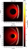 |
Fig. 6. Black hole disk images computed by GYOTO from the TITAN local angle dependent spectra, for two different spins. Images are computed at 6.4 keV and at θobs = 15° – almost face-on. The black hole mass is set to 108 M⊙. The map is created for monochromatic luminosity νLν in erg s−1 px−1, and the X and Y axes are in units of rg with the SMBH center as the origin. |
We also present an almost edge-on accretion disk in Fig. 7. The bright elongated region observed on the right side of an accretion disk is primarily due to relativistic Doppler boosting, where emission from the approaching side of the disk is enhanced (the disk rotates clockwise as viewed by a face-on observer). In addition, general relativistic light bending allows photons emitted from the other side of the disk, behind the black hole, to be redirected toward the observer. However, the flux observed from this lensed region is significantly lower than the direct disk emission, as only a small fraction of photons are bent along paths that reach the observer at a given θobs.
3.2.2. The influence of viewing angle and spin
To further study the various scenarios, we present the spectra of iron line regions for different spins (a) and viewing angles (θobs) in Figs. 8 and 9, respectively. In all those simulations, the iron line complex is self-consistently given by photoionization modeling with TITAN radiative transfer code. The effective emitting area of the disk increases with increasing black hole spin, since rISCO moves inward for higher spin values, as illustrated in Fig. 6. This trend directly affects the total luminosity, which is reflected in the position of the spectral continuum: for zero spin, the continuum strength is weakest, and it progressively increases with spin as seen in both Figs. 8 and 9.
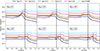 |
Fig. 8. The reflected ray-traced spectra from TITAN+GYOTO computations, for viewing angles (θobs) of the range from 5° to 30° given in the panel’s boxes. For each θobs, different line colors are plotted according to the spin values, displayed in the box above the figure. All spectra are presented by luminosity νLν versus photon energy E. The vertical dashed line marks the position of 6.4 keV energy. |
The dashed lines in Fig. 8 and Fig. 9 highlight the 6.4 keV energy in the observer’s frame. We do not see a neutral emission line for the initial data generated from TITAN in most of our scenarios, with a few exceptions at the outer edge of our radial structure. The major contribution to the observed 6.4 keV spectral feature comes from the Fe Kα emission lines of FeXXV and FeXXVI ions generated at 6.63, 6.67, 6.682, 6.7 keV for FeXXV and 6.957 keV for FeXXVI (see Sect. 3.3 for details). The high temperature of the matter structure is adequate for the existence of the highly ionized iron ions, whereas neutral iron does not exist under those physical conditions. Due to the close proximity to the SMBH, the emission from the highly ionized iron ions is gravitationally redshifted. For angles below 20°, we observe that the lines are redshifted around the 6.4 keV region. In contrast, for θobs greater than 20°, the line shift prominently moves out of this region, as seen on the lower panels of Fig. 8 and all panels of Fig. 9.
The motion of matter in an accretion disk around an SMBH introduces Doppler broadening and blue boosting of the emission lines. For θobs beyond 20°, the lines become extremely broadened due to disk motion, and at a maximal angle of 85°, the spectral features disappear in the underlying continuum, as presented in the lower right panels of Fig. 9. We also observe a noisier spectrum in Fig. 9. Since GYOTO traces rays backward from the screen to the disk, some rays may miss the disk, especially at high θobs, when the disk appears more edge-on. As a result, we see more numerical noise at these angles. Nevertheless, with increasing resolution, errors are suppressed.
The high θobs also produces a noticeable change in the spectrum continuum. In Fig. 9, we observe a rapid decrease in the continuum beyond the angle of 70°. The general relativistic light bending allows photons emitted from the far side of the disk, behind the black hole, to be redirected toward the observer. However, the flux observed from this lens region is significantly lower than the direct disk emission, as only a small fraction of photons are bent along paths that reach the observer at a given θobs, decreasing the overall continuum of the disk. Hence, the total line strength peaks around the region of 6.4 keV for lower θobs, approximately less than 20°, beyond which the contribution to the 6.4 keV region is not significant, and the peak moves either to higher energies or is completely smeared out.
3.2.3. The influence of lamp height and dissipation fraction
The position and energetics of the hot lamp and warm corona also determine the final line profile. The top panel in Fig. 10 shows how the relativistically corrected Fe Kα line profiles respond to changes in the lamp height. Only slight differences are observed in the line shapes, indicating that h has a relatively weak impact on the iron line shape. To understand the reason behind these small changes, we plotted the corresponding incident X-ray flux radial profiles FX(r) as a function of lamp height in the bottom panel of Fig. 10. Although there are minor changes in the flux level, the inversion in FX(r) appears around 10 rg, consistent with the emissivity profile discussed by Wilkins & Fabian (2012). This behavior arises due to the underlying formalism, where the lamp height only affects the FX(r) function, which in turn changes ξ(r), as defined in Eqs. (5) and (9), respectively (Ballantyne 2017).
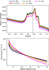 |
Fig. 10. Top panel shows the variation of the Fe Kα profile with the lamp height. The other parameters are set to their canonical values as shown in Table 2. The bottom panel shows the illuminating X-ray flux radial profiles, varying with the lamp height. The height is in units of rg given in the box above panels. |
We also see the variation of the energy flux distribution between the dissipative fraction fW and incident X-ray flux fraction fX in Fig. 11 and Fig. 12, respectively. The variation of fW gives the notion of the variation of the internal heating, which signifies the dissipative nature of the warm corona, while the variation of fX represents the variation of the incident X-ray flux incoming from the compact hot corona above the SMBH.
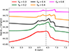 |
Fig. 11. Variation of the Fe Kα line profile with the dissipation fraction in the warm corona. The other parameters are set to their canonical values as shown in Table 2. |
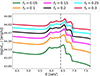 |
Fig. 12. Variation of the Fe Kα line profile with the illuminating X-ray flux fraction. The other parameters are set to their canonical values as shown in Table 2. |
As we assume the energy flux D(r) is varied between fX and fW, if fW is varied, then the back illumination’s contribution also changes, where fX is kept constant. Hence, as we change fW, we see in Fig. 11 how the contribution of internal heating affects the Fe Kα line profile. With no internal heating of the warm corona, i.e., fW = 0, thermal lines are still produced, as the temperature of the disk atmosphere is high enough to contain a large amount of highly ionised iron ions. With an increase of fW, we see the variation in the contribution of FeXXV and FeXXVI. As fW reaches higher values, the temperature of the matter structure rises, which ionizes FeXXV to FeXXVI, and the contributions of FeXXVI increase. For an fW = 0.8, the FeXXV is almost fully ionized to FeXXVI, and hence we only observe the double-peaked contribution of the FeXXVI ions. The detailed contribution of different iron line transitions to the total observed line profile is discussed in the section below.
A similar trend is also observed when we vary fX, while fW is kept constant. The FeXXV ions with an increase in fX ionize and the strength of FeXXVI increases. By increasing the emitting flux from the lamp, we observe an increase in the position of the continuum with the relativistically corrected Fe Kα profile. Hence, studying the variation in the highly ionized Fe Kα profile in AGN sources can help constrain the nature of the dissipative warm corona and the incident illumination strength. We also note that changes in the X-ray flux fraction fX or the lamp height h over time can give insights into the reverberation studies of accreting black hole systems. That is, the time-dependent changes in the reflected X-ray spectrum of the accretion disk, especially in the highly ionized Fe Kα line, show how the disk responds to changes in the lamp above the SMBH.
3.3. Contribution from different line transitions
The contribution of the Fe Kα lines that are emitted locally to the total observed line profile is depicted in Fig. 13 for a nearly face-on disk and six different spin values given in the boxes. With an increase in spin, the strength of the Fe Kα line emitted due to FeXXVI at 6.957 keV increases, which is expected due to the rise in total temperature of the matter structure as shown in Fig. 3. The contribution of FeXXV ions dominates most of the line profile, leading to the peak of the broad line structure at 6.4 keV for θobs = 15°. Their shift is similar, as these lines are generated very close to each other. A slight shift in their strength can be seen, suggesting that the temperature is adequate for the matter structure to generate more FeXXV ions at the energies 6.63 keV and 6.667 keV, which correspond to the forbidden and intercombination lines, respectively (see Bianchi et al. 2005). For spin 0.998, we see that the line structure has three distinctive peaks (bottom right panel of Fig. 13). Due to the high spin of the SMBH, the surrounding matter is heated to extremely high temperatures, leading to significant ionization. As a result, FeXXV ions become further ionized to FeXXVI, giving rise to a distinctive sharp peak for FeXXVI ions.
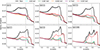 |
Fig. 13. Contribution of major Fe Kα lines to the total observed line profile is plotted by the solid black line. Lines emitted locally at 6.63 keV (cyan), 6.667 keV (green), 6.682 keV (orange), and 6.7 keV (brown) are contributions from the different ionization states of FeXXV, while the line at 6.957 keV (red) is the contribution from the FeXXVI ion. The continuum level is arbitrarily lumped together for better visualization. Different panels are for various spin values marked in the boxes, all for θobs = 15°. The vertical dashed line marks the position of 6.4 keV energy. |
Figures 14 and 15 show the contribution of the highly ionized iron lines for a rotating black hole with a = 0.9 but across θobs from 5° to 30°, and from 40° to 85°, respectively. The line profiles match the predictions in the literature (e.g., Fabian et al. 2000; Dauser et al. 2010). The effect of the tangential velocity of the disk is less at θobs = 5° compared to 85°. Hence, with the increase in angle, the rotational Doppler effect starts to dominate, and the lines become broadened. The peaks corresponding to the lines of the highly ionized ions FeXXV and FeXXVI are very close to each other for lower θobs, and are smeared into one peak. However, with increasing angle, FeXXVI, which originates further in energy than the FeXXV ions, starts to show a distinctive peak from θobs ≈ 40°. Beyond this angle, the Doppler effect is strong due to rotation, causing the lines to smear out.
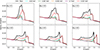 |
Fig. 14. Same as in Fig. 13 but for the single spin value of 0.9, and θobs in the range from 5° to 30° given in the panel’s boxes. |
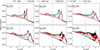 |
Fig. 15. Same as in Fig. 13 but for the single spin value of 0.9, and θobs in the range from 40° to 85° given in the panel’s boxes. |
The outer radius of the disk for two-zone geometry is arbitrarily chosen in this paper. A natural question arises about fluorescent line emission from outer disk radii, where the warm corona ends, and reflection from a cold disk may happen (see Fig. 2, lower right panel). This so-called cold iron line may contribute as an additional component to the total broad line profile seen by the distant observer. In Appendix B, we clearly show that due to the radial emissivity profile interpolated from TITAN calculations, the cold iron line has a negligible contribution to the total line profile. For a complete explanation of the broad iron line profile, we wish to physically define the transition radius between two-zone (warm corona or cold disk) and one-zone (cold disk) accretion flows. This issue will be the focus of our future research.
4. Discussion and conclusion
In this paper, we demonstrate that the broad feature typically observed in AGNs around 6.4 keV also has contributions from highly ionized Fe Kα lines. This can be modeled by ray-traced emission from a two-slab system containing a warm corona on the top of a cold disk, which is externally illuminated by hard X-ray power-law radiation from a lamp located above the central black hole. The inner region of the disk, surrounded by a warm corona, is fully dissipative and reaches very high temperatures at a large optical depth, in line with recent theoretical and observational predictions (e.g., Xiang et al. 2022; Gronkiewicz et al. 2023; Palit et al. 2024). Under such high temperatures, iron is highly ionized (Ballantyne 2020), and the emission lines corresponding to these ions, the so-called iron line complex, are created at local energies higher than 6.4 keV. Nevertheless, due to the close vicinity of the SMBH, these lines broaden and become gravitationally redshifted. Depending on the observer’s viewing angle, the highly ionized Fe Kα lines produced in the warm atmosphere may shift near 6.4 keV, and all of them partially participate in the total broad line profile. For this paper, we decided to concentrate only on line broadening due to relativistic effects, while Compton broadening will be included in the next step of our studies.
We considered 2D matter stratification to investigate the relativistic effects on highly ionized Fe Kα iron lines generated from FeXXV and FeXXVI ion populations. The radial solution adopted was taken from Xiang et al. (2022) and Ballantyne et al. (2024), where it was used to formulate the reXcor model to reproduce the soft X-ray excess widely observed in AGNs. In the reXcor model, local reflected spectra have been computed using a photoionization code designed by Ross & Fabian (1993) and later modified by Ballantyne et al. (2001). We follow this approach; nevertheless, for the solution of the matter structure and radiation transfer, we used the TITAN code by Dumont et al. (2003). It was demonstrated that TITAN is appropriate for matter under broad ionization conditions and being additionally heated by internal gain of energy, as required in the warm corona (Petrucci et al. 2020; Palit et al. 2024).
Our study shows the case of AGNs with a SMBH of the assumed mass 108 M⊙, and with a disk of mass accretion rate equal to 0.1 in units of Eddington accretion rate. According to the radial model used, the total energy flux generated due to accretion is fractionally distributed among three regions: hot lamp, warm dissipative corona, and cold disk. We show the dependence of the highly ionized Fe Kα features on the intrinsic parameters: spin, viewing angle, lamp height, dissipative fraction, and illuminating X-ray flux fraction.
The central SMBH spin plays a significant role in shaping the matter structure and influencing the relativistic shifts of emission lines, since we assume that the inner edge of the accretion disk is located at the rISCO, given solely by the spin. As the spin increases, the line profile becomes more pronounced and often exhibits a more distinctive peak structure. Although this may seem counterintuitive, the primary cause of these changes is not the variation in disk rotation, but rather the alteration in the disk’s vertical temperature structure, thereby changing the strength of the local emission from the highly ionized Fe Kα. The SMBH’s spin has minimal impact on disk rotation at large radial distances, but it becomes crucial in the innermost regions near the SMBH, by increasing the emitting surface with relatively high temperature that ensures a large FeXXV and FeXXVI ion population. This is a crucial factor as the temperature is heavily spin-dependent. Hence, for higher temperatures, the contribution from the FeXXVI ion increases, giving rise to a distinctive peaky structure in the line spectrum.
As expected, the viewing angle (θobs) of the observer plays an important role in the overall observed spectral shape. For a lower observing angle, the line shift is prominent at 6.4 keV, but with an increase in angle, the broad lines extend beyond 6.4 keV. At high θobs (above ∼30°), the lines are affected by extreme relativistic effects. Hence, for low θobs, the broad lines observed near 6.4 keV (see Guainazzi et al. 2006) in AGNs may contribute to the signatures of broadened and relativistically redshifted iron lines emitted from the FeXXV and FeXXVI ion populations.
We also investigated the lamp height and the distribution of the total energy flux. We reported that the lamp height did not show a significant change in the iron line profile. Hence, we studied how the illuminating X-ray flux changes with the height of the lamp. We noticed that the flux tends to pivot around a radial distance of about 10–20 rg. This means that when the lamp is close to the SMBH, the inner regions of the disk receive more X-ray light than the outer parts. This happens due to strong gravitational effects that bend the light more toward the center, as shown in Eq. (5). However, when the lamp is placed high above the black hole, the effect of gravity is weaker. As a result, the flux spreads more evenly and decreases smoothly with distance from the center.
On the other hand, the changes in the fractions of the energy flux distribution among the three regions have a significant effect on the iron line profiles. The increase of internal heating in the warm corona first results in a higher contribution from FeXXV, and further heating ionizes FeXXV to FeXXVI. This shows that effects such as changes in viscosity or magnetic field strength that induce changes in the dissipation of the warm atmosphere can highly affect the iron line profile. We also observe a strong correlation between the X-ray illumination and the iron line profile. An increase in the X-ray flux emitted from the lamp alters the profile of the iron line, particularly affecting the relative contributions of FeXXV and FeXXVI. This reflects how variations in the internal properties of the lamp can induce changes in the accretion disk that resemble reverberation effects. Although we focus here solely on the broad Fe Kα feature, and a direct analysis of reverberation is beyond the scope of this study, the observed changes in the line profile may still serve as a useful diagnostic of the lamp’s influence on the X-ray spectrum.
Numerous studies have shown the presence of the broad iron line structure in X-rays for different AGN sources (e.g., Fabian et al. 2000; Guainazzi et al. 2006; Miller 2007, and references therein). One of the best candidates showing a broad emission line in its X-ray spectrum is MGC-6-30-15(Tanaka et al. 1995). In a qualitative comparison, we see that our results for viewing angles of 20° −30° match the MGC-6-30-15 dataset shown in Fig. 4 of Miller (2007). In Iwasawa et al. (1996), a disk line is fitted assuming an angle of 30° obtained from Tanaka et al. (1995). These results show a strong resemblance to the scenario in which highly ionized iron ions are redshifted and contributing near the 6.4 keV region.
We note that in our work we have included the relativistic effects, but as a limitation of TITAN, we have not included the effects of Comptonization on the microscopic level. We are aware that multiple Compton scatterings of the line originating from dense matter can modify the final line profile; nevertheless, for this paper, we aimed to clearly show only one phenomenon that changes the line profile, which is strong gravity. Adding a proper treatment of Compton scattering will be included in our future work. The next important limitation of our model is the position of an outer cold disk from which the reflection may also occur and contribute to the overall spectrum. In the current model, we do not consider the reflection from the cold outer disk, since according to our studies (see Appendix B), the final line profile will be fully dominated by the emission from the inner disk’s warm corona region. We note that the above conclusion depends on the transition radius between a two-zone disk plus corona accretion flow and a one-zone cold disk. In this paper, only one arbitrarily assumed radial transition was considered. In our future work, we plan to develop a physically consistent model in which the warm corona can build up on the top of a cold disk, and the above transition will be self-consistently determined. This paper presents a complete method that can be used as soon as we can change the transition radius. Moreover, reverberation studies will be possible in such a complete model.
Contrary to the assumption of soft excess as an ionized standard disk emission (García & Kallman 2010; García et al. 2011, 2014), we assume that the disk has an additional heating component. We adopt the radial profile of internal heating from Xiang et al. (2022), while noting that the physical origin of the dissipative nature of the warm corona is possibly linked to magnetic fluxes, which have been discussed by Gronkiewicz et al. (2023). The deviation of the radial dependence of the emissivity profile from the standard disk assumption (as depicted in Appendix B) may also show the warm corona has a dissipative nature. We also show the importance of including the relativistic effects from the emission of the warm corona, which is also discussed by García et al. (2014). Hence, the broad line component observed in the X-ray spectrum can be described by emission from the warm corona.
We also aim to study further the effect of the mass, accretion rate, viscosity parameter, the radiative efficiency, and finally the matter structure on the emitted iron line profile. In future work, we aim to build a larger parameter space with larger constraints to compare it with the upcoming data from observatories like XRISM and NewATHENA. Broad iron line profiles have already been observed in multiple AGN sources (e.g., Reeves et al. 2001; Pounds et al. 2001; Guainazzi et al. 2006). We aim to develop a model that offers better parameterization for constraining the spin, mass, and viewing angles of SMBHs in AGNs.
Acknowledgments
PPB has been fully and AR has been partially supported by the Polish National Science Center grant No. 2021/41/B/ST9/04110. All computations have been performed using our computer cluster at NCAC PAS. DL acknowledges the Czech Science Foundation (GAČR) grant no. 25-16928O. We would like to thank David Ballantyne, Xin Xiang (Cindy), and Biswaraj Palit for their insightful comments on the paper.
References
- Adhikari, T. P. 2019, Photoionization Modelling as a Density Diagnostic of Line Emitting/Absorbing Regions in Active Galactic Nuclei (Cham: Springer International Publishing) [Google Scholar]
- Alcubierre, M. 2008, Introduction to 3+1 Numerical Relativity (Oxford, UK: Oxford University Press) [Google Scholar]
- Andonie, C., Bauer, F. E., Carraro, R., et al. 2022, A&A, 664, A46 [NASA ADS] [CrossRef] [EDP Sciences] [Google Scholar]
- Arnaud, K. A. 1996, in Astronomical Data Analysis Software and Systems V, eds. G. H. Jacoby, & J. Barnes, ASP Conf. Ser., 101, 17 [NASA ADS] [Google Scholar]
- Ballantyne, D. R. 2017, MNRAS, 472, L60 [NASA ADS] [CrossRef] [Google Scholar]
- Ballantyne, D. R. 2020, MNRAS, 491, 3553 [NASA ADS] [CrossRef] [Google Scholar]
- Ballantyne, D. R., Ross, R. R., & Fabian, A. C. 2001, MNRAS, 327, 10 [Google Scholar]
- Ballantyne, D. R., Sudhakar, V., Fairfax, D., et al. 2024, MNRAS, 530, 1603 [NASA ADS] [CrossRef] [Google Scholar]
- Baumgarte, T. W., & Shapiro, S. L. 2010, Numerical Relativity: Solving Einstein’s Equations on the Computer (Cambridge University Press) [Google Scholar]
- Bianchi, S., & Matt, G. 2002, A&A, 387, 76 [NASA ADS] [CrossRef] [EDP Sciences] [Google Scholar]
- Bianchi, S., Matt, G., Nicastro, F., Porquet, D., & Dubau, J. 2005, MNRAS, 357, 599 [Google Scholar]
- Boissay, R., Ricci, C., & Paltani, S. 2016, A&A, 588, A70 [NASA ADS] [CrossRef] [EDP Sciences] [Google Scholar]
- Dauser, T., Wilms, J., Reynolds, C. S., & Brenneman, L. W. 2010, MNRAS, 409, 1534 [Google Scholar]
- Dauser, T., Garcia, J., Wilms, J., et al. 2013, MNRAS, 430, 1694 [Google Scholar]
- Done, C., Davis, S. W., Jin, C., Blaes, O., & Ward, M. 2012, MNRAS, 420, 1848 [Google Scholar]
- Dumont, A. M., Abrassart, A., & Collin, S. 2000, A&A, 357, 823 [NASA ADS] [Google Scholar]
- Dumont, A. M., Collin, S., Paletou, F., et al. 2003, A&A, 407, 13 [NASA ADS] [CrossRef] [EDP Sciences] [Google Scholar]
- Fabian, A. C., Rees, M. J., Stella, L., & White, N. E. 1989, MNRAS, 238, 729 [Google Scholar]
- Fabian, A. C., Iwasawa, K., Reynolds, C. S., & Young, A. J. 2000, PASP, 112, 1145 [NASA ADS] [CrossRef] [Google Scholar]
- Falanga, M., Bakala, P., La Placa, R., et al. 2021, MNRAS, 504, 3424 [Google Scholar]
- Fukumura, K., & Kazanas, D. 2007, ApJ, 664, 14 [NASA ADS] [CrossRef] [Google Scholar]
- García, J., & Kallman, T. R. 2010, ApJ, 718, 695 [CrossRef] [Google Scholar]
- García, J., Kallman, T. R., & Mushotzky, R. F. 2011, ApJ, 731, 131 [CrossRef] [Google Scholar]
- García, J., Dauser, T., Lohfink, A., et al. 2014, ApJ, 782, 76 [Google Scholar]
- Gates, D. E. A., Truong, C., Sahu, A., & Cárdenas-Avendaño, A. 2025, Phys. Rev. D, 111, 124004 [Google Scholar]
- George, I. M., & Fabian, A. C. 1991, MNRAS, 249, 352 [Google Scholar]
- Gliozzi, M., & Williams, J. K. 2020, MNRAS, 491, 532 [Google Scholar]
- Gourgoulhon, E. 2007, arXiv e-prints [arXiv:gr-qc/0703035] [Google Scholar]
- Grevesse, N., & Anders, E. 1989, in Cosmic Abundances of Matter, ed. C. J. Waddington, AIP Conf. Ser., 183, 1 [Google Scholar]
- Gronkiewicz, D., Różańska, A., Petrucci, P.-O., & Belmont, R. 2023, A&A, 675, A198 [NASA ADS] [CrossRef] [EDP Sciences] [Google Scholar]
- Guainazzi, M., Bianchi, S., & Dovčiak, M. 2006, Astron. Nachr., 327, 1032 [NASA ADS] [CrossRef] [Google Scholar]
- Guilbert, P. W., & Rees, M. J. 1988, MNRAS, 233, 475 [Google Scholar]
- Iwasawa, K., Fabian, A. C., Reynolds, C. S., et al. 1996, MNRAS, 282, 1038 [NASA ADS] [CrossRef] [Google Scholar]
- Jiang, J., Fabian, A. C., Dauser, T., et al. 2019a, MNRAS, 489, 3436 [NASA ADS] [CrossRef] [Google Scholar]
- Jiang, Y.-F., Blaes, O., Stone, J. M., & Davis, S. W. 2019b, ApJ, 885, 144 [NASA ADS] [CrossRef] [Google Scholar]
- Kallman, T. R., & McCray, R. 1982, ApJS, 50, 263 [NASA ADS] [CrossRef] [Google Scholar]
- Laor, A. 1991, ApJ, 376, 90 [Google Scholar]
- Liedahl, D. A. 2005, in X-ray Diagnostics of Astrophysical Plasmas: Theory, Experiment, and Observation, ed. R. Smith (AIP), AIP Conf. Ser., 774, 99 [Google Scholar]
- Lightman, A. P., & White, T. R. 1988, ApJ, 335, 57 [NASA ADS] [CrossRef] [Google Scholar]
- Luminet, J. P. 1979, A&A, 75, 228 [Google Scholar]
- Madej, J., & Różańska, A. 2000, A&A, 363, 1055 [NASA ADS] [Google Scholar]
- Martocchia, A., & Matt, G. 1996, MNRAS, 282, L53 [NASA ADS] [CrossRef] [Google Scholar]
- Matt, G., Perola, G. C., & Piro, L. 1991, A&A, 247, 25 [NASA ADS] [Google Scholar]
- Miller, J. M. 2007, ARA&A, 45, 441 [NASA ADS] [CrossRef] [Google Scholar]
- Miniutti, G., & Fabian, A. C. 2004, MNRAS, 349, 1435 [NASA ADS] [CrossRef] [Google Scholar]
- Nandra, K. 2006, MNRAS, 368, L62 [NASA ADS] [CrossRef] [Google Scholar]
- Nandra, K., George, I. M., Mushotzky, R. F., Turner, T. J., & Yaqoob, T. 1997, ApJ, 477, 602 [NASA ADS] [CrossRef] [Google Scholar]
- Nandra, K., O’Neill, P. M., George, I. M., & Reeves, J. N. 2007, MNRAS, 382, 194 [NASA ADS] [CrossRef] [Google Scholar]
- Nayakshin, S., Kazanas, D., & Kallman, T. R. 2000, ApJ, 537, 833 [NASA ADS] [CrossRef] [Google Scholar]
- Palit, B., Różańska, A., Petrucci, P. O., et al. 2024, A&A, 690, A308 [NASA ADS] [CrossRef] [EDP Sciences] [Google Scholar]
- Petrucci, P. O., Paltani, S., Malzac, J., et al. 2013, A&A, 549, A73 [NASA ADS] [CrossRef] [EDP Sciences] [Google Scholar]
- Petrucci, P. O., Ursini, F., De Rosa, A., et al. 2018, A&A, 611, A59 [NASA ADS] [CrossRef] [EDP Sciences] [Google Scholar]
- Petrucci, P. O., Gronkiewicz, D., Rozanska, A., et al. 2020, A&A, 634, A85 [NASA ADS] [CrossRef] [EDP Sciences] [Google Scholar]
- Pounds, K. A., Nandra, K., Stewart, G. C., George, I. M., & Fabian, A. C. 1990, Nature, 344, 132 [NASA ADS] [CrossRef] [Google Scholar]
- Pounds, K., Reeves, J., O’Brien, P., et al. 2001, ApJ, 559, 181 [NASA ADS] [CrossRef] [Google Scholar]
- Reeves, J. in Active Galactic Nuclei: From Central Engine to Host Galaxy, eds. S. Collin, F. Combes, & I. Shlosman, ASP Conf. Ser., 290 [Google Scholar]
- Reeves, J. N., Turner, M. J. L., Pounds, K. A., et al. 2001, A&A, 365, L134 [NASA ADS] [CrossRef] [EDP Sciences] [Google Scholar]
- Reis, R. C., & Miller, J. M. 2013, ApJ, 769, L7 [NASA ADS] [CrossRef] [Google Scholar]
- Ross, R. R., & Fabian, A. C. 1993, MNRAS, 261, 74 [NASA ADS] [CrossRef] [Google Scholar]
- Różańska, A., Czerny, B., Życki, P. T., & Pojmański, G. 1999, MNRAS, 305, 481 [CrossRef] [Google Scholar]
- Różańska, A., Dumont, A. M., Czerny, B., & Collin, S. 2002, MNRAS, 332, 799 [CrossRef] [Google Scholar]
- Różańska, A., Malzac, J., Belmont, R., Czerny, B., & Petrucci, P. O. 2015, A&A, 580, A77 [NASA ADS] [CrossRef] [EDP Sciences] [Google Scholar]
- Shakura, N. I., & Sunyaev, R. A. 1973, A&A, 24, 337 [NASA ADS] [Google Scholar]
- Svensson, R., & Zdziarski, A. A. 1994, ApJ, 436, 599 [NASA ADS] [CrossRef] [Google Scholar]
- Tanaka, Y., Nandra, K., Fabian, A. C., et al. 1995, Nature, 375, 659 [NASA ADS] [CrossRef] [Google Scholar]
- Vincent, F. H., Paumard, T., Gourgoulhon, E., & Perrin, G. 2011, Class. Quant. Grav., 28, 225011 [NASA ADS] [CrossRef] [Google Scholar]
- Vincent, F. H., Różańska, A., Zdziarski, A. A., & Madej, J. 2016, A&A, 590, A132 [NASA ADS] [CrossRef] [EDP Sciences] [Google Scholar]
- Wilkins, D. R., & Fabian, A. C. 2012, MNRAS, 424, 1284 [NASA ADS] [CrossRef] [Google Scholar]
- Xiang, X., Ballantyne, D. R., Bianchi, S., et al. 2022, MNRAS, 515, 353 [NASA ADS] [CrossRef] [Google Scholar]
- Yaqoob, T., Edelson, R., Weaver, K. A., et al. 1995, ApJ, 453, L81 [NASA ADS] [Google Scholar]
Appendix A: Single line test
Here we present the results for the single line test, where we inject a 6.9 keV Gaussian function with the flat continuum at all the disk radii. This scenario is unrealistic as the line flux is kept constant throughout the disk radial structure with an arbitrary value of the equivalent width of 600 eV. We aimed to show that the inclusion of relativistic effects on the highly ionized Fe Kα line may contribute to the broad line profile observed at the energy of the neutral (6.4 keV) line.
Fig. A.1 shows the relativistically corrected spectrum for the case of a non-spinning SMBH, varying with the viewing angle θobs. We observe the profiles to follow a similar structure as described in Dauser et al. (2010) and Gates et al. (2025). For a low viewing angle, the shift of the line from the 6.9 keV (marked with a dashed vertical line in Fig. A.1) to the energy of the neutral fluorescent line (dash-dotted vertical line in Fig. A.1) is observed. Additionally, with a low θobs, we see a high continuum flux as more photons reach us from a face-on view, which is also consistent with the previous results (e.g., Fabian et al. 2000). The line shape broadens with an increase in θobs as the tangential component of the rotational velocity contributes more, which leads to extreme line broadening. Single line test shows the correctness of the GYOTO code, but it does not include a proper radial emissivity profile of a line flux. It corresponds to the disk line models of Fabian et al. (1989) and of Laor (1991) that are available in the commonly used XSPEC fitting package (Arnaud 1996). To study the realistic emissivity profile of the iron line complex together with the underlying continuum, we used a combination of TITAN and GYOTO, as described in Sec. 3.
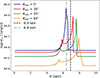 |
Fig. A.1. Spectrum generated by GYOTO for various viewing angles, computed for an injected single Gaussian line with μ = 6.9 keV and σ = 10 eV. The computations have been made for a non-spinning black hole with 108 M⊙, and for an integration disk surface from rin = rISCO + 1 to rout = 25 rg. The equivalent width was chosen as 600 eV and was kept constant at all radii. The vertical dashed black line depicts the 6.9 keV, while the vertical dash-dotted gray line depicts 6.4 keV. |
Appendix B: Reflection from an external cold disk
The two-zone geometry, which includes the warm, optically thick corona above the cold disk, ends on an arbitrarily chosen outer radius 25 rg. Since we do not know the physical mechanism that causes the warm corona disappearance, we decided not to explore this parameter in the current paper. We plan to explore this issue towards a complete solution of the disk + corona geometry. Nevertheless, we should not completely forget about the reflection from the outer cold disk and eventual production of the fluorescent iron line. Hence, to test here the contribution from the outer region of the disk, we appended additional disk rings up to 100 rg. The local emission from those rings contains a continuum with a Gaussian-like shape of emission line originating from a fluorescent process. We tested the contribution for the outer region in the case of a non-rotating SMBH, i.e., a = 0.
As a starting point, we have to estimate the radial emission profile (EP) up to the outer radius 100 rg. To extract EPs, we take radial flux values of reflected spectra calculated by TITAN code for different emission angles and extrapolate them to larger radii by fitting the following emissivity law:
 (B.1)
(B.1)
where K is a power-law normalization constant, and n is an emissivity power-law index. We plot the EPs resulting from TITAN code by a solid line in Fig. B.1, where we choose continuum flux at 6.8 keV as a reference point. The region where the warm corona is dominated by Compton cooling is seen by the strong radial bump in the emissivity. This may be a potential radial size of a warm corona, but we plan to explore this issue in our future research. The bump decreases with radius, and the EP given by Eq. (B.1) is fitted to the last 5 points, which depict the region where line cooling starts to dominate, as discussed in Sec. 3.1. For all the profiles, we found that the best-fit for emissivity follows a profile close to r−3, which depicts the EP for a standard (Wilkins & Fabian 2012). The best fit values for each emission angle are shown in Tab. B.1.
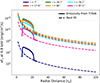 |
Fig. B.1. Variation of the flux emitted at 6.8 keV with the radial distance. The computations were done for different emission angles (i) prescribed in TITAN. |
Best fit parameters for the angle-dependent Emissivity Profile given by Eq. (B.1), and depicted in Fig. B.1. Here i is the emission angle from TITAN. The best-fit parameter is computed for the continuum emission at 6.8 keV.
Further, we construct the continuum for the radial range 25-100 rg with 50 points in between using the reflected continuum at 25 rg to follow the best fit power law of EP. Then we add a 400 eV line at each within this radial distance. In this way, we created an expected level of continuum and line spectra for the outer cold disk region (i.e., without a warm corona). The dependence of continuum levels and lines on radii for the case of emission angle i = 17.6° is presented in Fig B.2. The fluorescence iron line at 6.4 keV is visible as a reflection from outer radii.
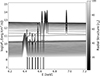 |
Fig. B.2. Output spectrum from TITAN added with the spectra of the best fit parameters beyond 25 rg. The 6.4 keV line is injected with a 400 eV equivalent width. This figure is depicted for the emission angle i = 17.6°. |
The final ray-traced spectrum is computed after integration of the emission up to 100 rg. The contribution of each iron transition to the total broad observed feature is presented in Fig. B.3, similar to Sec. 3.3. Cold iron line (depicted by green dashed line) has a negligible impact on the final broad iron line profile. Hence, the two-zone (warm corona on the top of a cold disk) region within 25 rg is extremely important, which contributes to the formation of the broad iron line spectrum. More cases will be considered in our future papers when the radial extension of the warm corona will be self-consistently defined.
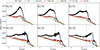 |
Fig. B.3. Contribution of the individual lines to the total line profile computed for different angles. The depicted colors are the same as Fig. 13, with the addition of light green showing the contribution from the 6.4 keV fluorescent iron line. |
Appendix C: Comparison to the reXcor model
We compare our results (TITAN+GYOTO) to the reXcor model; however, we note that there are significant differences between the two models: we mainly aim to model the line profiles, but reXcor is designed to study the soft excess, thus the line profile in it is computed as angle-averaged. With GYOTO, we compute the viewing angle-dependent emission spectrum. In Fig. C.1, we show different panels corresponding to the emission spectra produced for different viewing angles θobs from our model, and compare them to the angle-integrated reXcor profile. Our emission spectra for θobs = 10° and 20° show some similarities to the angle-averaged spectrum produced by reXcor. For larger viewing angles, we observe that the line is broadened out of the range of the line profile produced by reXcor.
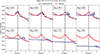 |
Fig. C.1. Angle-averaged emission spectrum from reXcor versus the viewing angle-dependent spectrum from our model (dark blue lines). The panels depict different viewing angles, as indicated in the top-left corner of each panel. The red line corresponds to the spectrum from reXcor. The model parameters are selected to be consistent with reXcor, and they are indicated in the plot header. The vertical dashed line represents the 6.4 keV region. |
We also calculate that the angle-averaged flux,
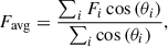 (C.1)
(C.1)
where Fi is the flux observed at viewing angle θi. The comparison of the angle-averaged emission spectrum of our model and reXcor is depicted in Fig. C.2. We observe that the angle-averaged emission spectrum aligns with the output from reXcor, with minor differences in the peak. These differences in the peak suggest a difference in the assumption of the physical process considered in reXcor. The peaks at around 6.5 keV do match in Fig. C.1 for the θobs = 20°, but disappear in the angle averaging. Hence, we note that the angle-averaged emission spectrum for TITAN+GYOTO is computed via summation of discrete angles, which may give rise to a spectrum with high errors observed as a bumpy line spectrum in Fig. C.2. We also note that the inclusion of Comptonization gives an estimate of soft excess, while with TITAN+GYOTO, we only model the lines and not the soft excess. Hence, below approximately 4 keV, the continuum mismatch can be seen.
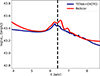 |
Fig. C.2. Comparison of the emission spectrum from the angle-averaged data from our model (dark blue) and the reXcor model (red). The vertical dashed line represents the 6.4 keV region. |
All Tables
Best fit parameters for the angle-dependent Emissivity Profile given by Eq. (B.1), and depicted in Fig. B.1. Here i is the emission angle from TITAN. The best-fit parameter is computed for the continuum emission at 6.8 keV.
All Figures
|
Fig. 1. A schematic diagram of our model’s setup. A hot corona, as in lamppost geometry, is located at height h above the SMBH of mass M and spin a. The warm corona is positioned on top of an accretion disk. The incident flux coming from the hot corona is reprocessed in the warm corona, which is then detected by the observer. The rin and rout are the integration limits for our model. We compute the vertical structure using TITAN with the input parameters depicted in the warm corona panel; Γ – photon index, ξ – ionization parameter, NH – column density, nH – gas number density, Q – internal heating, and TBB – the temperate of blackbody radiation from an underlying disk. |
| In the text | |
|
Fig. 2. Radial distribution of global model parameters that are inputs for TITAN code. The colors represent different spin values given in the top box. The subplots are as follows: top left panel: gas number density (Eq. (1)), top middle panel: dissipation flux (Eq. (2)), top right panel: X-ray flux from a hot corona (Eq. (5)), bottom left panel: ionization parameter (Eq. (9)), bottom middle panel: internal heating of the warm corona (Eq. (10)), and bottom right: accretion disk temperature TBB (Eq. (11)). The vertical dashed lines mark the radius at which the output temperature structure from TITAN reaches the maximum, see Fig. 3 and text for details. |
| In the text | |
|
Fig. 3. Temperature dependence on the optical depth for various spin values given in the boxes. The gray gradient of lines represents the matter structure calculated at different radii, with the darkest line at rin, and the lightest line at rout. The colored lines show the simulation with maximum temperature, which is consistent with the dashed line in Fig. 2. The corresponding radial point where the temperature drop is observed is labeled and marked in green text. The parameters other than spin are chosen to be canonical values from Table 2. As this is the temperature structure, it is independent of the viewing angle. |
| In the text | |
|
Fig. 4. Heating and cooling of the matter structure at equilibrium for spin 0 and mass 108 M⊙. The plots depict different points of the radial structure, left: 20.538, middle: 21.385, right: 22.231 rg. The solid lines depict heating and the dashed lines depict cooling. |
| In the text | |
|
Fig. 5. Local spectra νFν versus photon energy E, from TITAN code, for different spin values at the i = 17.6°. The gray gradient of lines depicts outgoing spectra calculated at different radii, with the darkest line at rin, and the lightest line at rout. The colored lines show the simulation with maximum temperature, which is coherent with the dashed line in Fig. 2 and solid colored lines in Fig. 3. The parameters other than the spin and the viewing angle are set to be canonical values as depicted in Table 2. |
| In the text | |
|
Fig. 6. Black hole disk images computed by GYOTO from the TITAN local angle dependent spectra, for two different spins. Images are computed at 6.4 keV and at θobs = 15° – almost face-on. The black hole mass is set to 108 M⊙. The map is created for monochromatic luminosity νLν in erg s−1 px−1, and the X and Y axes are in units of rg with the SMBH center as the origin. |
| In the text | |
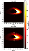 |
Fig. 7. Same as in Fig. 6 but for θobs = 70° – almost edge-on. |
| In the text | |
|
Fig. 8. The reflected ray-traced spectra from TITAN+GYOTO computations, for viewing angles (θobs) of the range from 5° to 30° given in the panel’s boxes. For each θobs, different line colors are plotted according to the spin values, displayed in the box above the figure. All spectra are presented by luminosity νLν versus photon energy E. The vertical dashed line marks the position of 6.4 keV energy. |
| In the text | |
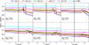 |
Fig. 9. Same as in Fig. 8, but for θobs for the range from 40° to 85° given in the panel’s boxes. |
| In the text | |
|
Fig. 10. Top panel shows the variation of the Fe Kα profile with the lamp height. The other parameters are set to their canonical values as shown in Table 2. The bottom panel shows the illuminating X-ray flux radial profiles, varying with the lamp height. The height is in units of rg given in the box above panels. |
| In the text | |
|
Fig. 11. Variation of the Fe Kα line profile with the dissipation fraction in the warm corona. The other parameters are set to their canonical values as shown in Table 2. |
| In the text | |
|
Fig. 12. Variation of the Fe Kα line profile with the illuminating X-ray flux fraction. The other parameters are set to their canonical values as shown in Table 2. |
| In the text | |
|
Fig. 13. Contribution of major Fe Kα lines to the total observed line profile is plotted by the solid black line. Lines emitted locally at 6.63 keV (cyan), 6.667 keV (green), 6.682 keV (orange), and 6.7 keV (brown) are contributions from the different ionization states of FeXXV, while the line at 6.957 keV (red) is the contribution from the FeXXVI ion. The continuum level is arbitrarily lumped together for better visualization. Different panels are for various spin values marked in the boxes, all for θobs = 15°. The vertical dashed line marks the position of 6.4 keV energy. |
| In the text | |
|
Fig. 14. Same as in Fig. 13 but for the single spin value of 0.9, and θobs in the range from 5° to 30° given in the panel’s boxes. |
| In the text | |
|
Fig. 15. Same as in Fig. 13 but for the single spin value of 0.9, and θobs in the range from 40° to 85° given in the panel’s boxes. |
| In the text | |
|
Fig. A.1. Spectrum generated by GYOTO for various viewing angles, computed for an injected single Gaussian line with μ = 6.9 keV and σ = 10 eV. The computations have been made for a non-spinning black hole with 108 M⊙, and for an integration disk surface from rin = rISCO + 1 to rout = 25 rg. The equivalent width was chosen as 600 eV and was kept constant at all radii. The vertical dashed black line depicts the 6.9 keV, while the vertical dash-dotted gray line depicts 6.4 keV. |
| In the text | |
|
Fig. B.1. Variation of the flux emitted at 6.8 keV with the radial distance. The computations were done for different emission angles (i) prescribed in TITAN. |
| In the text | |
|
Fig. B.2. Output spectrum from TITAN added with the spectra of the best fit parameters beyond 25 rg. The 6.4 keV line is injected with a 400 eV equivalent width. This figure is depicted for the emission angle i = 17.6°. |
| In the text | |
|
Fig. B.3. Contribution of the individual lines to the total line profile computed for different angles. The depicted colors are the same as Fig. 13, with the addition of light green showing the contribution from the 6.4 keV fluorescent iron line. |
| In the text | |
|
Fig. C.1. Angle-averaged emission spectrum from reXcor versus the viewing angle-dependent spectrum from our model (dark blue lines). The panels depict different viewing angles, as indicated in the top-left corner of each panel. The red line corresponds to the spectrum from reXcor. The model parameters are selected to be consistent with reXcor, and they are indicated in the plot header. The vertical dashed line represents the 6.4 keV region. |
| In the text | |
|
Fig. C.2. Comparison of the emission spectrum from the angle-averaged data from our model (dark blue) and the reXcor model (red). The vertical dashed line represents the 6.4 keV region. |
| In the text | |
Current usage metrics show cumulative count of Article Views (full-text article views including HTML views, PDF and ePub downloads, according to the available data) and Abstracts Views on Vision4Press platform.
Data correspond to usage on the plateform after 2015. The current usage metrics is available 48-96 hours after online publication and is updated daily on week days.
Initial download of the metrics may take a while.