| Issue |
A&A
Volume 707, March 2026
|
|
|---|---|---|
| Article Number | A162 | |
| Number of page(s) | 20 | |
| Section | Interstellar and circumstellar matter | |
| DOI | https://doi.org/10.1051/0004-6361/202557159 | |
| Published online | 17 March 2026 | |
A surprisingly large asymmetric ejection from Mira A
1
Department of Space, Earth and Environment, Chalmers University of Technology,
412 96
Gothenburg,
Sweden
2
Escuela de Física, Universidad Nacional Autónoma de Honduras, Ciudad Universitaria,
Tegucigalpa,
Honduras
3
School of Physics and Center for Relativistic Astrophysics, Georgia Institute of Technology,
837 State Street,
Atlanta,
GA
30332,
USA
4
European Southern Observatory, Alonso de Córdova,
3107
Vitacura,
Santiago,
Chile
5
Rosseland Centre for Solar Physics, University of Oslo,
PO Box 1029 Blindern,
0315
Oslo,
Norway
6
Institute of Theoretical Astrophysics, University of Oslo,
PO Box 1029 Blindern,
0315
Oslo,
Norway
7
School of Physics & Astronomy, Monash University,
Wellington Road,
Clayton
3800,
Victoria,
Australia
★ Corresponding author: This email address is being protected from spambots. You need JavaScript enabled to view it.
Received:
9
September
2025
Accepted:
19
January
2026
Abstract
Context. Stars with masses between roughly 1 and 8 M⊙ end their lives on the asymptotic giant branch (AGB), when intense mass loss takes place, with major consequences for the chemical evolution of the universe. The mechanism responsible for the outflows is generally accepted to be radiation pressure acting on dust grains that form in the dense extended atmospheres of AGB stars. Dust formation is enabled, or at least dramatically enhanced, by the action of convection and stellar pulsations. The complex physics underlying convection, stellar pulsations, and dust nucleation precludes predicting AGB mass loss from first principles.
Aims. Our aim was to characterize the recent mass ejections of the AGB star Mira A using observations of the inner envelope. In particular, we studied two lobes observed to be expanding away from Mira A to obtain empirical insights into the mass-ejection process.
Methods. We investigated the evolution of the lobes using images of polarized light obtained at six epochs using the Spectro-Polarimetric High-contrast Exoplanet REsearch (SPHERE) on the Very Large Telescope and of molecular emission at two epochs obtained with the Atacama Large Millimeter/submillimeter Array (ALMA). Six lines of SO2 were used to investigate the excitation temperature and column density of SO2 in the lobes. We used the 13CO J = 3-2 line and radiative transfer models to constrain the column density of the gas, which allowed us to infer the abundances of SO, SO2, AlO, AlF, and PO in the lobes.
Results. While dust seems confined almost exclusively to the edges of the lobes, gas fills the lobes and displays higher densities than expected at the observed radial distances based on the large-scale mass-loss rate of Mira A, with a total gas mass in the lobes of ∼2 × 10⁻⁵ M⊙. We find the expansion of the lobes to be consistent with both a constant velocity (ejection time in 2010 or 2011) or a decelerating expansion (ejection time in 2012). If ejection events with a similar magnitude happen periodically, we derive periods between 50 and 200 years to account for the mass-loss rate of Mira A. This periodicity is very uncertain because of the complexity of the circumstellar environment that hampers accurate determinations of the mass-loss rate. We find abundances in the lobes of ∼1.5 × 10⁻⁶ and ∼2.5 × 10⁻⁶ for SO and SO2, respectively, when accounting for radiative transfer effects and of 2 × 10⁻¹⁰, 6.5 × 10⁻¹⁰, and 4 × 10⁻⁷ for AlO, AlF, and PO assuming LTE and optically thin emission. The strong variation in brightness of the different features identified in the polarized-light images is puzzling. We suggest that an asymmetric stellar radiation field preferentially illuminates specific regions of the circumstellar envelope at a given time, producing a lighthouse-like effect.
Key words: stars: AGB and post-AGB / circumstellar matter / stars: mass-loss / stars: individual: omicron Ceti / stars: winds, outflows
© The Authors 2026
 Open Access article, published by EDP Sciences, under the terms of the Creative Commons Attribution License (https://creativecommons.org/licenses/by/4.0), which permits unrestricted use, distribution, and reproduction in any medium, provided the original work is properly cited.
This article is published in open access under the Subscribe to Open model. This email address is being protected from spambots. You need JavaScript enabled to view it. to support open access publication.
1 Introduction
The asymptotic giant branch (AGB) represents one of the last phases of the evolution of low- and intermediate-mass stars, with initial masses between ∼1 and ∼8 M⊙. During the AGB, stars are cool and have sizes that are more than two orders of magnitude larger than on the main sequence, and a structure that consists of a compact dense core surrounded by a large convective envelope (Herwig 2005). Stellar pulsations excited in the envelope and convective motions cause the atmosphere to be out of hydrostatic equilibrium, and to have a larger density scale height. In this dense, cool, extended atmosphere, atoms can form molecules and, if the partial pressures are high enough, dust grains. The newly formed grains significantly affect the opacity in the region by absorbing and scattering radiation. The radiation pressure felt by the dust grains can affect the dynamics of the gas and dust mixture in the extended atmosphere significantly. If the radiation pressure force per mass element is stronger than the gravitational pull, material is accelerated outward (Höfner & Olofsson 2018). The outflows that develop in this way have mass-loss rates roughly between 10−8 and 10−4 M⊙ yr−1, and determine the fate of the star.
Predicting the mass-loss rate from first principles is not yet possible because of the complex interplay between convection, stellar pulsations, and dust formation and growth. The dust-formation process is especially difficult to understand in oxygen-rich AGB stars for which the carbon-to-oxygen number ratio is lower than one, and where dust nucleation is still a matter of debate (Plane 2013; Gail et al. 2016; Gobrecht et al. 2022, 2023). In these environments, the lack of dust species that are abundant and can survive at high temperatures (Woitke 2006) implies that relatively large grains (≳0.3 μm) are expected to drive the outflow mainly through the scattering of radiation (Höfner 2008). Despite the complex context, wind-driving models have made significant advances in the last decades. For instance, calculations of convection and dust growth in threedimensional models now allow for the evolution of ejected filaments to be studied in simulations (Höfner & Freytag 2019; Freytag & Höfner 2023).
Our empirical knowledge has also improved significantly, thanks to the advance in instrumentation. Specifically, high angular resolution instruments now allow for the direct study of the region where dust forms and grows and the wind is accelerated. The detection of grains within the expected size range around AGB stars (Norris et al. 2012; Ohnaka et al. 2017; Khouri et al. 2020) using these techniques with NaCo and the Spectro-Polarimetric High-contrast Exoplanet REsearch (SPHERE) on the Very Large Telescope (VLT) has provided support for this mass-loss paradigm. In particular, the emerging picture is of an inner circumstellar structure consisting of a gravitationally bound shell containing aluminum oxide grains surrounded by a region where silicate formation happens and the outflow is triggered (Karovicova et al. 2013; Khouri et al. 2015; Höfner et al. 2016).
In addition, the Atacama Large Millimeter/submillimeter Array (ALMA) and near-IR interferometry allow the dynamics of the gas in the extended atmospheres to be studied in unprecedented detail (Vlemmings et al. 2017; Khouri et al. 2018; Ohnaka et al. 2019; Khouri et al. 2024; Ohnaka et al. 2024). The very high angular resolution achieved in such observations reveals structures imprinted on the stellar photospheres by convective cells that are spatially resolved (Paladini et al. 2018; Vlemmings et al. 2024) and hotspots on the extended atmospheres that remain largely unexplained (Vlemmings et al. 2015, 2017). On larger scales, observations of molecular emission have also revealed new features of ejection and shaping mechanisms of the outflow. For instance, the clumpy ejections observed in the carbon-rich AGB star CW Leo have been hypothesized to be produced by convective motions (Velilla-Prieto et al. 2023), while the complex morphologies on intermediate scales observed in a sample of oxygen-rich AGB stars were suggested to originate from interactions with companions (Decin et al. 2020).
In this context, we report observations with ALMA of molecular emission arising from the inner circumstellar environment of the AGB star in the binary system o Ceti, Mira A. These observations reveal the expansion of gas and dust in lobes that increase in extent from ∼10 au to ∼40 au from Mira A between 2015 and 2023. In particular, we studied in detail two lobes with enhanced molecular emission first reported by Khouri et al. (2018). We also analyzed light scattered by dust observed using SPHERE on the VLT that arises from the edges of such lobes. In Sects. 2 and 3, we present the observations and the results obtained from the analysis of the data, respectively. In Sect. 4, we present radiative transfer models guided by the results given in Sect. 3. In Sect. 5, we discuss our results, while our conclusions are summarized in Sect. 6.
2 Observations
For the molecular line emission, we used data obtained with ALMA on 2017 November 9 and 2023 July 6 and 14 at high angular resolution in the context of projects 2017.1.00191.S and 2022.1.01071.S. The spatial resolutions achieved in the observations of these projects are ∼17 (2017.1.00191.S) and ∼15 milliarcseconds (mas; 2022.1.01071.S). We also employed lower spatial resolution (0″.2) data from project 2018.1.00749.S obtained on 2018 November 26 to investigate whether a significant amount of flux is not recovered by the interferometer in the 2017 observations. The data obtained in 2017 were reduced and presented by Khouri et al. (2018), and we refer to that study for details of the data reduction process. The datasets from 2018 and 2023 were reduced using the standard ALMA pipeline by the observatory. We retrieved the reduced cubes through the ALMA archive. The maximum recoverable scales estimated by the ALMA observatory and listed in the archive are 0″.329, 3″.033, and 0″.433 for the data obtained in 2017, 2018, and 2022, respectively.
The observations of polarized light were acquired using the ZIMPOL sub-instrument (Schmid et al. 2018) of SPHERE on the VLT in the context of individual projects and guaranteed-time observations. We searched the archive of the European Southern Observatory and retrieved data obtained using the CntHa filter on 2015 September 23, 2016 October 12, 2018 October 10, 2021 January 3, and 2023 July 21 and the NR filter on 2017 November 27. The data were reduced using the pipeline developed at ETH Zurich including bias subtraction, flat-field correction and modulation-demodulation-efficiency correction (Schmid et al. 2018), with the adoption of values for the modulation-demodulation efficiency of 0.8 when the fast readout mode was employed (2016 October 12, 2017 November 27, 2021 January 3, and 2023 July 21) and 0.9 when the slow mode was used (2015 September 9 and 2018 October 10).
The spatial resolution in the ZIMPOL images depends on the performance of the adaptive optics and can be measured using the full width at half maximum (FWHM) of the point spread function (PSF). The performance is strongly influenced by the atmospheric conditions and the brightness of the source, and can produce FWHM as narrow as ∼15 mas in optimal cases (Schmid et al. 2018). When a reference point source was observed close in time to the images of the Mira system (two epochs), the reference images were used to determine the FWHM of the PSF. Alternatively, Mira B can be used as a PSF reference even if it has a low brightness compared to Mira A. In Table 1, we give the measurement of the FWHM of Mira B and the other PSF reference (del Cet), when available. The resolution in the SPHERE images presented by us varies between ∼19 mas and ∼28 mas.
All images are shown with coordinates relative to the position of Mira A (α = 02h19m20s.79 and δ = -02°58′39″.496). The moment-zero maps of the lines shown below are obtained by averaging the channels that show emission. Throughout the paper, we consider a systemic velocity of Mira A with respect to the local standard of rest of υLSR = 47 km s−1. The pulsation period of Mira A is ∼332 days (Samus’ et al. 2017) and we use the maximum of the light curve around May 5, 2015 as the zero-phase reference.
Stellar pulsation phase at the time of the ZIMPOL observations and spatial resolution in the obtained images.
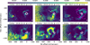 |
Fig. 1 Images of the polarization degree (color map) toward Mira at different epochs in filters CntHa for all epochs except for 2017, which was observed with filter NR. The approximate pulsation phases (φ) of Mira A at the times of the observations are given above each panel. The white contours show the total intensity emission from Mira A at 20%, 40%, and 80% of the peak value. The red dots mark the position of the companion in the total intensity images, while the gray dots in the bottom right panel indicate the approximate position of the companion in previous epochs. The straight line used to determine the reference point on the NE lobe is shown in the upper middle panel. The 3σ contour of the SO JK = 88 - 77 emission in 2017 November (shown in Fig. 2) is marked by the magenta line in comparison to the polarized-light map at the same epoch. The gray ellipse in the bottom right corner of each panel indicates the full width at half maximum of the point spread function in the obtained images. |
3 Observational results
A complex structure with two prominent lobes is observed in both the polarized light images (Fig. 1) and the maps of molecular line emission (Fig. 2 and additional maps throughout the paper). In addition to the lobes, a feature to the south of Mira A that seems to curve to the east toward Mira B can be seen in the polarized-light images, but it has at most a weak counterpart in the molecular line data, as seen in the SO emission to the south of Mira A (Fig. 2). The lobes are by far the most conspicuous structures in the molecular line maps. The presence of these lobes were reported by Khouri et al. (2018) based on single-epoch observations (data from 2017 also included in this study). The authors noted that the dust producing the scattered light seems to be confined mostly to the edge of the molecular emission lobes. When the observations at other epochs are considered, the evolution of the lobes becomes clear, with expansion visible both in the polarized light images (Fig. 1) and in the molecular emission maps (Fig. 2).
3.1 Scattered light
The polarized light images shown in Fig. 1 reveal a complex dust distribution in the system. In particular, the edges of the lobes are traced. The images acquired in 2015 and 2021 reveal that dust in the lobe to the north-east (NE lobe) of Mira A is mostly confined to a shell. The images show the NE lobe to expand significantly over the timespan of the observations we report, ∼8 years. A lobe to the north-west (NW lobe) is not seen as clearly at all epochs. We speculate that this is caused by the different orientation of the two lobes. Given that the NW lobe is too faint in most epochs for its morphological evolution to be assessed, we only use the polarized light images to quantify the expansion of the NE lobe.
The size of the NE lobe at each epoch was measured using the position of a reference point relative to the center of Mira A. The reference point was chosen as the intersection of the centre of the filament with a straight line making a 30° angle with the west-east direction and passing through the center of Mira A (see Fig. 1). We consider the measurement uncertainty to be half of the width of the filament at a given epoch, or a larger width from a previous epoch. This was motivated by the facts that the surface brightness distribution of the filament and its width vary significantly as a function of time, which is probably caused by the varying strength of the signal from the filament between the different epochs, rather than an actual variation in its width. Independently of the cause, this hampers a more precise identification of a reference point. The obtained radial positions as a function of time are shown in Fig. 3.
Using the function CURVE_FIT of the SciPy Python module, we fitted two functions to the measured points, a straight line representing constant expansion and a ballistic trajectory assuming a mass of 1.2 M⊙ for Mira A. For the constant-expansion model, we obtain the expansion velocity of the NE lobe on the plane of the sky,  , and its corresponding projected radial extent at the reference epoch (Sep 23, 2015),
  . We find
  = 10.5 ± 1.6 km s−1 and
  = 12.3 ± 0.8 au. Extrapolating backward implies that the NE lobe would have been located at Mira A’s surface 1650 ± 200 days before the first SPHERE observations (Sep 23, 2015), suggesting an ejection date between late 2010 and early 2011. For the ballistic model, the two free parameters are the ejection velocity,
  , and the ejection time,
  . We obtain
  = 31.6 ± 0.6 km s−1 and
  = 980 ± 150 days before September 23, 2015, which corresponds to an ejection time in late 2012 or early 2013. As shown in Fig. 3, both models fit the observations well, preventing us from precisely concluding what the initial velocity and time of the ejection of the NE lobe were.
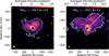 |
Fig. 2 Moment-zero maps of the emission in the SO JK = 88–77 line observed in 2017 November 9 and 2023 July 6 and 14. The approximate pulsation phases (φ) of Mira A at the times of the observations are given at the top of each panel. The white contours mark where emission reaches three times the RMS noise level in each image. The straight white line in the right panel indicates the direction used to measure the size of the NW lobe in the two epochs. |
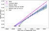 |
Fig. 3 Observed distance on the plane of the sky of the reference point of the NE (maroon circles) and NW (magenta squares) lobes. The magenta solid line and blue dashed line show the fits to the observed extents of the NW and NE lobes, respectively, assuming constant expansion. The magenta dot-dashed and green dotted line shows a fit to the extent of the NW and NE lobes, respectively, assuming a ballistic trajectory for a star with 1.2 M⊙. The black intervals mark the uncertainty interval on the ejection times of the lobe to the NE based on the two models. |
3.2 Molecular emission in the lobes
The molecular emission traces the two lobes clearly both in November 2017 and in July 2023. However, the size of the lobes in 2023 is larger than the maximum recoverable scale of the ALMA array used for the observations, which likely leads to a significant loss of flux. In the observations acquired in 2017, several lines reveal the lobes, as noted by Khouri et al. (2018). To characterize the emission in the lobes, we use 9 lines (Table 2) from four different molecules: CO, 13CO, SO, and SO2. Additionally, we use one line of AlO, AlF, and PO to estimate the abundances of these molecules in the lobes. Throughout the text, we do not specify the atomic mass and the vibrational state when referring to the main isotopes of each atom and to transitions within the ground vibrational state, respectively.
A particularly good tracer of the lobe is the SO JK = 88 − 77 line (Fig. 2), because this line is optically thick in the lobes, as discussed below. Intrinsically stronger lines, such as 29SiO J = 8-7, show that lower-density gas surrounds the lobes. As discussed in Sect. 5.4, we estimate the gas surrounding the lobes to have a density about one order of magnitude lower if the excitation temperatures and abundances in the two regions are not significantly different. In the second epoch, emission in the SO JK = 88 − 77 line becomes weaker relative to the noise level, which remains basically the same at the two epochs, at ∼0.5 mJy/beam. This is caused both by an intrinsic decrease in the surface brightness with the expansion of the lobes and an observational effect due to loss of flux (see Sect. 3.2.2). Because of the weaker emission and larger emission region size with respect to the beam in 2023, we use the observations from 2017 to derive the physical properties of the gas in the lobes.
Properties of the lines used to study the lobes.
3.2.1 Expansion of the NW lobe
To estimate the projected expansion velocity of the NW lobe,  , in a similar way as done for the NE one, we measured the position of its edge using a straight line in the north-west direction passing through the center of Mira A (Fig. 2). Our reference point is defined by the interception of this line with the edge of the molecular lobe, which we define as the contour at three times the root-mean square (RMS) noise level of the molecular emission maps. We use both the SO JK = 88 − 77 and 13CO J = 3-2 emission maps averaged over the line profiles. For the images from 2017, the two lines yielded sizes that differed by only 5%, and we used the average as a representative value. For the images from 2023, we used only the SO JK = 88 − 77 maps because the emission of the 13CO J = 3-2 line was weak compared to the RMS noise level and did not produce continuous contours. With this approach, we obtain the two magenta points shown in Fig. 3. A fit of a straight line (constant velocity) implies
  ∼ 12.4 km s−1 and
  ∼ 14.9 au. Hence, the edge of the NW lobe would have been at the surface of Mira A ∼1785 days before the reference epoch (Sep 23, 2015), which corresponds to an ejection time around late 2010. Considering a ballistic trajectory, we find ejection velocity,
  , and the ejection time,
  , equal to ∼33 km s-1 and 1090 days before 23 September, 2015, respectively, implying an ejection time in mid or late 2012.
The values for the NW lobe are more uncertain than those for the NE one, because of the smaller number of measurements and the less robust method for measuring a reference point at the edge of the lobe.
3.2.2 Resolved-out emission
To estimate whether a significant amount of flux was resolved out in the observations of the low-excitation lines acquired in 2017, we used the products available in the ALMA archive from project 2018.1.00749.S. These data were acquired on 2018 November 26, which is close to one year after the observations we analyze in this study and cover the lines 13 CO J = 32, SO Jκ = 88−77, AlO N = 9-8 and SO2 JKa,Kc = 43,1−32,2, 212,20−211,21, and 343,31−342,32. The achieved spatial resolution is significantly lower, with a beam size of 0″.25 × 0″.19 and a position angle varying between -71° and -77°.
To compare both datasets, we use the IMSMOOTH function in CASA to smooth the higher-resolution image cubes from 2017 to the same resolution as the 2018 ones, using the appropriate beam size and orientation at the frequency of each line. Then, we extract spectra from both datasets using a circular region with diameter 0″.4 centered on the continuum peak. As shown in Fig. A.1, the lines have very similar strengths in both epochs. The only line displaying strong variation is AlO N = 9-8, which is almost a factor of two weaker in 2018. This could be caused by dissociation or a change in the excitation of the molecule. Based on this comparison, we conclude that there is no significant loss of flux in the observations from 2017 despite the relatively small beam.
3.2.3 SO2 population diagrams
We identify six relatively strong lines of SO2 (Table 2) in the spectra of the data obtained in November 2017. The energies of the upper level of these lines range between ∼31 and ∼985 K, covering the expected gas temperatures in the region probed. Hence, these are excellent for tracing the excitation temperature,  , and column density, NSO2, of SO2 molecules in the lobes.
To retrieve the excitation temperature and column density of SO2 per pixel, we averaged the emission in these six SO2 lines over frequency to obtain the so-called moment-zero maps of the lines. These maps were then used to obtain a population diagram (Goldsmith & Langer 1999) for each pixel. To calculate the number of molecules in the upper level of each transition at each given pixel (Nu), we used the expression
 (1)
(1)
where d is the distance to the Mira system (∼100 pc, van Leeuwen 2007; Haniff et al. 1995), F is the flux of the given line in the given pixel, lpxl is the size at the distance of Mira corresponding to the angular size of the pixels, h is the Planck constant, and ν and Aul are the frequency and the Einstein-A coefficient of the relevant transition, respectively. The flux per pixel was obtained by dividing the flux per beam by the ratio between beam and pixel areas at the frequency of each line. The pixel size in the images produced by us corresponds to 3.6 mas, or 0.36 au at 100 pc, at all frequencies.
After obtaining values for the populations of the six levels for each pixel, we derived the excitation temperature and column density, N, per pixel by fitting straight lines to the data in the  plane, where gu and Eu are the degeneracy and excitation energies of the upper level, respectively. An example of such a fit is shown in Fig. D.10. The excitation temperature is equal to minus the inverse of the slope of the fitted line, while the column density is equal to the partition function at the relevant excitation temperature,
  , times the exponential of the intercept of the fitted line. We used the partition function as a function of temperature provided by Underwood et al. (2016) and available through the ExoMol database.
To calculate the uncertainties in the derived quantities, we used a Monte Carlo method and simulated 3 × 10⁴ observations. In each simulation, the line fluxes per pixel were randomly chosen from Gaussian distributions centered on the values of the given pixel of the moment zero maps and with standard deviations equal to the observed root-mean square noise of the given map. We do not include the absolute flux calibration uncertainty in the estimate of the excitation temperature because that does not affect the relative strengths of the lines, which is used to determine the excitation temperature. We considered in our calculations all pixels for which the fluxes of at least four SO2 lines were higher than three times the root-mean square noise. The standard deviations on the determined values of  and NSO2 for each pixel were calculated based on the distributions of the 3 × 10⁴ values of
  and NSO2. The maps of the excitation temperature, column density, and the corresponding standard deviation are shown in Fig. 4. Integrating over the SO2 emission region, we obtain a total number of SO2 molecules ∼6.6 × 1045.
Based on the obtained temperature maps and channel-averaged emission of the SO2 lines, we calculated maps of the averaged optical depth for each line (Fig. D.2). Given that the averaged optical depth of the SO2 lines peaks at ∼0.5, optical depth effects are expected to affect the lines to some extent. Nonetheless, the derived excitation temperature distribution are also supported by our radiative transfer models discussed below, implying that these transitions provide a good probe of the SO2 excitation in this region.
3.2.4 Gas column densities
To translate the observed NSO2 values to gas column densities, the abundance of SO2 needs to be determined. This is not straightforward, however, because sulfur can be atomic, in molecules (mainly SO or SO2), and even in dust grains. Therefore, there is a large uncertainty on the SO2 abundance.
In light of this, we use the 13CO J = 3-2 line to estimate the gas column density and derive the SO2 abundance. The abundance of 13CO should be much better constrained, because virtually all 13C is expected to be locked in 13CO. To obtain the column density of 13CO molecules, we assume that the excitation temperature of the 13CO J = 3-2 line is the same as the one derived from the SO2 line. The simplest scenario in which this would be true is if all the lines in question are excited under LTE conditions. Our population diagram calculations for SO2 suggest that this is a likely possibility, given that a single excitation temperature produced very good fits to each pixel in both lobes. Moreover, the derived temperatures vary smoothly over the lobes. The relatively low value of the Einstein-A coefficient of the 13CO J = 3-2 line implies that collisions dominate the excitation for the gas densities we infer. The average optical depth of the 13CO J = 3-2 line in the lobes (Fig. 5) implies that the estimated column densities are a lower limit because of opacity effects. Nonetheless, we do not expect a strong effect in the lobes. We address the problem of the optical depths by calculating radiative transfer models below.
Under the assumption of optically thin emission and excitation temperature equal to that of SO2, we obtain the column density map shown in Fig. 5. As can be seen, the highest optical depths in the 13CO J = 3-2 line are reached in the innermost regions of the envelope, where densities are high. Hence, we expect strong optical depth effects to affect the measured column density of 13CO for regions at radii r < 60 mas from the center of Mira A.
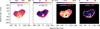 |
Fig. 4 Results from the SO2 populations diagram. From left to right, the panels show the obtained maps of |


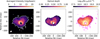 |
Fig. 5 Observed emission (left) and inferred optical depth (middle) of the 13CO J = 3-2 line and corresponding calculated column density of 13CO (right) assuming optically thin emission and the same excitation temperature distribution derived for SO2. The dashed white circle in the middle panel marks the 60 mas radius inside of which the derived column densities are not reliable because of high optical depths. The white and magenta contours in the left and right panels, respectively, mark emission equal to three times the RMS noise level. |
3.2.5 Estimated molecular abundances
Assuming a 13CO abundance relative to H2 of 3 × 10⁻⁵ (Hinkle et al. 2016; Khouri et al. 2018), our results imply an average abundance of SO2 with respect to H2 of −2.5 × 10 6 for r > 60 mas from the center of Mira A. As a reference, we consider the solar sulfur abundance with respect to H2 (~2.6 × 10⁻⁵, Asplund et al. 2021) to be an upper limit to possible values of sulfurbearing molecules. Similarly, we estimated the abundances of other molecules with strong line emission in the lobes using the lines SO 88−77 (Fig. D.3), AlF J = 10-9 (Fig. D.4), AlO J = 98 (Fig. D.5) and PO 2Π3/2 J = 8-7 (Fig. D.6) and the excitation temperatures and gas column densities derived above using the SO2 and 13CO lines. As before, we consider only the emission arising from r > 60 mas. The partition function and transition parameters adopted from the literature for each molecule are specified in Appendix C. We find average abundances of ~4.5 × 10⁻⁷ for SO, of 6.5 × 10⁻¹⁰ for AlF, of 2 × 10⁻¹⁰ for AlO, and 4 × 10⁻⁷ for PO. While emission in most lines is overall optically thin, the SO JK = 88−77 line reaches high optical depths in the lobes, implying that the abundance derived in this way represents only a lower limit. The radiative transfer calculations discussed below provide a better estimate of the abundance. The J = 8-7 line of 29SiO was also inspected by us, but the optical depths in this line are so high that estimating an abundance associated with the emission has little meaning.
4 Radiative transfer models for the molecular lines
To better constrain the morphology, abundances, and density and velocity distributions of the gas in the lobes, we calculated radiative transfer models using the code LIME (Brinch & Hogerheijde 2010). The model output consists of a line emission cube for each line. These cubes were convolved to the resolution of the observations at the central frequency of each transition. The stellar continuum was subtracted to produce continuum-free model line cubes. The modeled spectra were extracted using circular apertures centered on the model star and with radii equal to 40 mas, 100 mas, and 200 mas. These were compared to spectra extracted from the same regions from the observed data (Fig. 8).
4.1 Model setup
We base the structure of the model on the results presented in Sect. 3 and on the model for r < 84 mas around Mira A presented by Khouri et al. (2018). The stellar temperature (T* = 2100 K) and radius of the central star at 338 GHz, R*338 GHz = 21.25 mas (or 2.125 au at 100 pc), were adopted from Vlemmings et al. (2019). Since LIME does not include a central star explicitly, we include a central blackbody consisting of a dust-rich sphere that is optically thick at all wavelengths considered in the calculation and has a temperature equal to the brightness temperature of the central star at 338 GHz (2100 K).
For CO, rotational levels up to J= 40 in the ground, first, and second vibrational states are included. The collisional rates we use were obtained by Castro et al. (2017). The CO and 13CO abundances relative to H2 were kept fixed in the models at 4 × 10⁻⁴ and 3 × 10⁻⁵, respectively, following (Khouri et al. 2018), while the abundances of SO and SO2 were allowed to vary to fit the observed line strengths. In this way, the gas density in the lobes is constrained mostly by fitting the strength of the 13CO line extracted using different apertures, while the abundances of SO and SO2 are the most relevant parameters to match the strength of the lines of each species. The relative strengths of the SO2 lines together with the radial brightness distribution of each line are the main constraints for the gas temperature distribution.
4.1.1 Envelope physical structure
To approximate the structure of the inner circumstellar environment of Mira A, we consider a sphere (Inner Region) and two lobes described by truncated ellipsoids (Fig. 6). The radius of transition between the Inner Region and the lobes, Rtrans, was set to 91.375 mas (4.3 R*) based on the size of the bright ring seen in the 13CO J = 3-2 channel maps (Fig. D.8). The lobes are described by ellipsoids centered on Mira A and truncated at the intersection with a plane perpendicular to the major axis of the given lobe and located 2 R* away from the center of Mira A. This approach was chosen to avoid the lobes extending in front of the star because that would produce blueshifted absorption against the stellar continuum which is not observed in the spectral lines. The lobes envelop the Inner Region for radii smaller than 4.3 R*.
As a reference, we refer to the plane defined by the two major axes of the ellipsoids as the main plane of the model in the following description. As shown in Fig. 6, we oriented the major axis of the NE lobe 20° away from the x direction and toward the y direction on the main plane. For the NW lobe, the major axis was oriented 5° off the x = y direction toward the y axis on the main plane. This implies an angle of 110° between the two major axes of the lobes. These parameters were chosen to reproduce the morphology traced by the molecular lines (e.g., Fig. 7). The lobe to the NW was inclined toward the observer by an angle of 20° by rotating the main plane about the major axis of the NE lobe. This is necessary to reproduce the observed blueshifted emission in the channel maps (Fig. D.8).
The kinetic temperature, T, density, ρ, and velocity distributions of the gas were assumed to be power-law functions of the radial distance to the star. The gas density and temperature decrease radially and are described by one power-law function within the Inner Region and different ones in the lobes. The steepness and reference values of the functions were determined from the observations as detailed below. The gas velocity field has only a radial component, to which a turbulence velocity of 3 km s−1 is added. The lines are also affected by thermal broadening based on the local kinetic temperature.
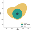 |
Fig. 6 Schematic view of the model with the different regions indicated. This view is a cut through the plane defined by the two major axes of the ellipses (main plane of the model). For the ray-tracing, the model is rotated about the major axis of the smaller lobe by an angle of 20°. In this way, the larger lobe is inclined toward the observer to produce the observed blueshifted emission. |
4.1.2 Model parameters and modeling approach
The good description of the level populations of SO2 using a single temperature for each pixel suggests that the obtained temperature values are good approximations to the average gas kinetic temperature along the line of sight, and that the populations of the corresponding SO2 levels are excited under LTE. Based on the obtained map, we adopt a continuous temperature profile that is equal to the observed continuum temperature at  (2100 K) and drops to 400 K at Rtrans = 4.3 R* (91.375 mas) and to 300 K at 10.4 R* (220 mas). This corresponds to a broken power law with exponents ~-1.14 for r < Rtrans and ~-0.33 for r > Rtrans.
We use the estimated radial decrease of the 13CO column density to assess the steepness of the gas density profile. For this, we consider only the regions over which the lobes have roughly constant width (up to r ~ 180 mas) to prevent effects from the narrowing of the lobes at the edges. We find the 13CO column density to decrease by less than a factor of two from the average value at r = 90 mas. This factor should not be strongly affected by the effect of the morphology of the lobes on the observed column densities and, hence, should be indicative of the steepness of the gas density profile, implying a weak dependence of the gas density with radius in the lobes. For a power-law distribution  , this implies η~-0.75. The velocity of the gas in the models is also described by a linear function of r,
  , where υin and υout are the velocities at the inner (Rin) and outer (Rout) radii of the given region. Negative and positive velocities correspond to infall and outflow, respectively. The velocity distribution was assumed to be on average negative in the inner spherical region and positive in the lobes, because of the redshifted absorption observed in the line profiles (Fig. 8) and of the measured outward expansion of the lobes, respectively.
The density and velocity distributions were varied from our initial model to reproduce the observed line emission. We compared the model predictions to the observed lines  and 36(5,31)−36(4,32) of SO2, JK = 88−77 of SO, and J = 3-2 of 13CO considering local thermodynamical equilibrium and from line v = 1, J = 3-2 of CO considering non-LTE effects. Although non-LTE effects can be important for the CO v = 1, J = 3-2 line, it is difficult to assess whether our calculations provide a good approximation for the radiative excitation, given the uncertain direct stellar radiation field as discussed below.
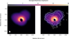 |
Fig. 7 Moment-zero map of the 13CO J = 3-2 line of the best-fitting model (color map) compared to the moment zero of the observed line (white contours at levels of 3, 5, 10, and 20 times the RMS noise). The line emission and physical structure of the same model are shown in Figs. 8 and 9, respectively. |
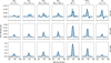 |
Fig. 8 Observed lines extracted from three different apertures (blue histograms) compared to the results from the radiative transfer model (dashed black lines) summarized in Table 3. A systemic velocity of 47 km s−1 was added to the model. |
4.2 Model results
As shown in Figs. 7 and 8, the observed lines are fairly well reproduced by a radiative transfer model with the parameters derived in Sect. 4.1.2 based on the population diagram analysis. The temperature, density and velocity profiles used in the model are summarized in Table 3 and shown in Fig. 9. To reproduce the weaker emission observed south of the star, we reduce the gas density in the Inner Region for y < R*, where y is the coordinate on the main plane of the model (Fig. 6), to the value at the base of the lobes (8 × 10¹⁴ H2 molecules m−3, Table 3). Additionally, the gas densities in the NE lobe are 30% lower than in the NW lobe at the same radial distance. This difference was introduced because otherwise the relative brightnesses of the lobe does not fit the observed emission maps.
The density needs to be relatively high (~1017 molecules/m3) close to the star for the CO v = 1, J = 3-2 line to be as strong as observed. A steep density distribution is required to reproduce the lower-excitation 13CO J = 3-2 emission arising from a larger region. The model contains gas masses of −8 × 10⁻⁵ M⊙ and ~2.1 × 10⁻⁵ M⊙ in the Inner Region and the lobes, respectively.
We find abundances of SO and SO2 in the lobes of −1.5 × 10⁻⁶ and −2.5 × 10⁻⁶, respectively. Our calculations also show that the abundance of SO2 in the high gas density region close to the star (r ≲ Rtrans) is likely significantly lower than in the lobes, with values −2 × 10⁻⁷, because otherwise the lines from the smallest aperture considered by us are predicted to be stronger than observed as shown in Fig. B.1. Our models also suggest a similar behavior for the SO abundances, but the high optical depths of the SO line in the Inner Region make constraining the SO abundance more difficult.
While the optical depths in the 13CO J = 3-2 line reach values of −1 in our models, the SOJK = 88−77 emission reaches higher values. Especially in the innermost regions (r ≤ Rtrans), strong optical depth effects are expected to affect these lines. The SO2 lines have average optical depths peaking at −0.5, which indicates some effects from opacity. Nonetheless, these transitions are not strongly affected by optical depth effects and our model confirms that they constitute a good probe of the excitation temperature and SO2 column density in the lobes.
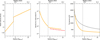 |
Fig. 9 Physical parameters of the radiative transfer model (yellow line) summarized in Table 3 and with fits to the observations shown in Fig. 8. The dashed red line shows the lower density in the NE lobe. The gray curve in the temperature panel shows a gray atmosphere temperature profile. The vertical light gray lines mark Rtrans. |
Results from the radiative transfer model.
5 Discussion
5.1 Gas density and temperature in the extended atmosphere
The model described in Sect. 4.2 and shown in Fig. 9 was tailored to reproduce the low-excitation lines. This requires making a compromise of not reproducing the strength of the absorption observed in the CO v = 1, J = 3-2 line. As discussed by Khouri et al. (2018), the relatively strong absorption feature in the CO v = 1, J = 3-2 line is an indication of this line tracing gas that is cool compared to the stellar continuum temperature. However, if we decrease the gas temperature in the innermost regions of the model to try to reproduce this feature, the absorption in the lower-excitation lines 13CO J = 3-2 and SO JK = 8877 becomes stronger. Therefore, we are not able to reproduce the strength of the absorption in all lines simultaneously, and we conclude that there are aspects of the physical properties of the gas in the extended atmosphere that are not captured by our model. We prioritize reproducing the low-excitation transitions, which are used to constrain the properties of gas in the lobes.
One possible way to explain this problem is a more complex distribution of gas with cool and warm components existing at the same distance from the star, which is different from our model in which the temperature is a function of only the radial distance. Such a structure is not unexpected and could correspond to gas in updrafts and downdrafts, or an overall clumpy structure, with gas having different properties at the same radius such as seen in three-dimensional hydrodynamical models (Freytag & Höfner 2023). Another possible explanation is that our model does not include the proper stellar radiation field to account for the non-LTE excitation of CO to excited vibrational states. Our approach for including the star in our model has the shortcoming that the stellar brightness temperature corresponds to the one observed in the continuum at 338 GHz (2100 K) and is the same at all frequencies. In reality, the radiation from deeper, hotter regions of the star probably contribute significantly to the radiation field at ∼2.3 and ∼4.6 μm, which is responsible for exciting CO to higher vibrational states. Despite this shortcoming, we deem it more important to include a star that provides the correct continuum brightness temperature at the frequencies of our observations because that has a direct effect on the amount of absorption in all lines.
Both the excitation temperature map and the radiative transfer calculations reveal a steep temperature profile close to the star, with temperatures as low as 600 K reached at r ~ 3 R* and 430 K at r ~ 4 R*. Such a steep temperature profile is in agreement with previous results which revealed cold gas close to the Mira A (Wong et al. 2016; Kaminski et al. 2017; Khouri et al. 2018), as well as similar results for other oxygen-rich AGB stars, such as R Dor and W Hya (Khouri et al. 2024; Vlemmings et al. 2017; Ohnaka et al. 2025). This indicates that low gas temperatures close to the star are a relatively common feature of oxygen-rich AGB envelopes. For comparison, the radius at which the temperature has dropped to ∼430 K is ∼9 times larger than where it reaches 2100 K in state-of-the-art three-dimensional hydrodynamic models of AGB stars (Freytag & Höfner 2023).
5.2 Velocity profile
We consider the determined velocity profile more uncertain than the density and temperature profiles. There are two main reasons for this. First, the velocity distribution in the model was only constrained using the line profiles as a function of aperture size, because we did not aim to reproduce the brightness distribution in individual velocity channels in detail. Second, the radial velocities and the turbulence in the gas both affect the line profiles and are somewhat degenerate in the models, with the turbulence also probably varying as a function of radius from the star. Hence, the exact shape of the velocity profile should be seen as a representative possibility rather than a full description, but its general characteristics, such as expanding outer lobes with maximum expansion between ∼12 km/s and an in-falling inner shell with average velocities –4 km/s, are trustworthy.
Additionally, the discontinuity in the profile at Rtrans does not necessarily represent a region of acceleration of the flow, as in a steady-wind scenario, but instead of the radial boundary between bodies of gas that experienced different kinematic histories.
5.3 Redshifted emission peak in the SO2 lines
In the spectra extracted from small apertures shown in Fig. 8, an emission component observed in the SO2 lines at velocities ∼58 km s−1 (∼11 km s−1 with respect to the systemic velocity of 47 km s−1) is not reproduced by the model. The SO line shows emission at similar velocities which might be produced by the same kinematic component of the envelope. At larger apertures, no additional emission is observed at those velocities except for that already present in the spectrum from the innermost region.
To determine the location of the gas producing this emission, we averaged the SO2  line over the five channels in which the emission is clearly seen. The resulting map is shown in Fig. 10. The emission arises from the direction where the CO v = 1, J = 3-2 emission also peaks (Fig. D.9).
In contrast to the CO v = 1, J = 3-2 line, SO2 JKa,Kc = 212, 20−211, 21 emission seems to be produced in front of the stellar disk, which is unexpected for cooler gas surrounding a hotter source. If emission arises from gas in front of the star, the observed red-shifted velocity would correspond to gas falling back to the star. Moreover, an excitation temperature higher than the brightness temperature of the star is expected for thermal emission in this case. However, the molecules responsible for this feature do not seem to have a particularly high excitation temperature because the feature is strongest in the SO2 JKa,Kc = 212, 20−211, 21 line with excitation energy of ∼219.5 K, and its strength decreases in the higher-excitation lines (see Fig. 8). If the emission arises from close to the stellar limb by gas located behind the star, it would be produced by outflowing material.
This feature could also be produced by stimulated emission in principle, if the excitation is non-thermal. However, it is probably unlikely that maser emission in several SO2 lines at similar velocities arises from the same region.
Vlemmings et al. (2017) and Ohnaka et al. (2025) also reported emission toward the stellar disk of the AGB star W Hya and attributed the lines to SO2 transitions. In the interstellar medium and in protostars, SO and SO2 are known as tracers of shocks (e.g., Pineau des Forets et al. 1993; Podio et al. 2015). A deeper understanding of whether these molecules also trace shocks in the inner regions of the circumstellar envelopes of AGB stars might provide new tools to studying these crucial innermost regions, where shocks and active chemistry affect the level populations of molecules. Such an investigation is beyond the scope of this study.
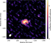 |
Fig. 10 Redshifted emission excess observed in the SO2 JKa,Kc = 212, 20−211, 21 line. The red circle represents the stellar disk observed in the continuum emission. The white contour marks emission above three times the RMS noise level. |
5.4 Recent mass-loss rate and ejection periodicity
We find that the ejections observed using ZIMPOL and ALMA must have taken place roughly between 5 and 7 years before the ALMA observations in November 2017 when considering expansion with deceleration or constant velocity, respectively. Since the expansion velocity evolution cannot be well constrained based on the observations we report, we are unable to constrain the ejection mechanism. The observations are consistent with either an energetic event that expelled gas at very high velocities or the standard dust-driven outflow with relatively fast acceleration to the current expansion velocities.
The density of the gas around the lobes can be estimated by assuming that the excitation temperatures and abundances are similar in the lobes and the gas surrounding them. The 29SiO abundance for solar composition is ∼1.6 × 10 6 without depletion, which is very similar to the value we derive for the SO abundance (∼1.5 × 10⁻⁶). Considering LTE excitation at a temperature ∼300 K, emission in the 29SiO J = 8-7 line is expected to be a factor of ten stronger than in the SO JK = 88−77 line given the difference in the value of the partition functions, energy levels, and Einstein-A coefficients of the two transitions. Therefore, the fact that we see weak emission in the 29SiO line surrounding the lobes but no emission in the SO line implies a gas density contrast ≲10 under these assumptions.
The fate of the ejected gas is not immediately clear because the material in the lobes might leave the system or not. At a distance of 20 au, the escape velocity from a star with 1 M⊙ is ∼9 km s−1. However, this value can easily be ∼12 km s−1 if the present-day mass of Mira A is higher (∼1.6 M⊙) or if Mira B is included in the calculation. Hence, the maximum inferred expansion velocities are tantalizingly close to the expected escape velocity, and the gas might not escape the system without an extra force, such as radiation pressure on dust. In fact, the derived initial velocity for the ballistic trajectory to the NE lobe (31.6 ± 0.6 km s−1) is within the possible range of escape velocities from the surface of Mira A, between ∼26 and 35 km s−1 for a present-day mass between 0.8 and 1.5 M⊙. This implies that gas following trajectories within the uncertainty would either narrowly escape the gravitational field of Mira A or not. For a 1.2 M⊙ star (with trajectories shown in Fig. 3), gas moving ballistically would expand to distances of at least ∼70 au before potentially falling back. In reality, the problem is complicated by the distribution of previously ejected gas in the circumstellar environment and the effect of Mira B. Additionally, even a relatively small amount of radiation pressure on dust would imply that the material indeed leaves the system. However, dust does not seem to be very abundant in the lobes, apart from in the edges, which puts to question whether the observed lobes are mostly driven by radiation pressure on dust, or created by an alternative ejection mechanism (e.g., Judge & Stencel 1991) with radiation pressure on dust playing only a supporting role. Observing the future evolution of the lobes should provide important clues to answering these questions.
It is possible to set constraints on the potential periodicity of ejections of this magnitude. In the case that all gas in the lobes leaves the system, events such as this would contribute to the mass lost by Mira A. However, determining the mass-loss rate and history of Mira A on larger scales is difficult because of the complexity introduced by the gravitational pull, radiation field, and high-velocity outflow of Mira B (Ramstedt et al. 2014). Nonetheless, analyses of CO lines indicate a relatively low value for the mass-loss rate of Mira A. Scaling values from the literature using the distance and CO abundance considered by us, we obtain 1.1 × 10⁻⁷, 1.5 × 10⁻⁷, 1.9 × 10⁻⁷, 4 × 10⁻⁷ M⊙ yr−1 from values available in De Beck et al. (2010), Planesas et al. (1990), Ryde & Schöier (2001), and Knapp et al. (1998), respectively. We note that the models from Ryde & Schöier (2001) and Planesas et al. (1990) have fairly low values for the expansion velocity (2.5 and 3.0 km s−1, respectively), which are at odds with the observed expansion velocity of the lobes. The results from De Beck et al. (2010) and Knapp et al. (1998) imply higher maximum expansion velocities (8.1 and 6.7 km s−1, respectively), which are more comparable to the values we infer for the lobes. In Knapp et al. (1998), the outflow of Mira A is divided into two components, one faster (6.7 km s−1) and the other slower, expanding at 2.4 km s−1 and accounting ∼18% of the total rate of mass loss.
On even larger scales, a tail seen in far-UV light likely produced by emission from collisionally excited H2 (Martin et al. 2007) is seen to extend ∼4 pc away from the system. Using the proper motion of the binary pair, Martin et al. (2007) derived that this tail corresponds to mass lost in the last 3 × 10⁴ years. However, hydrodynamical modeling revealed that the ejected gas is decelerated more slowly by the interstellar medium and that the tail might have been created over 4.5 × 10⁵ years instead (Wareing et al. 2007). Both works considered a mass-loss rate of 3 × 10⁻⁷ M⊙ yr−1 (or 2.6 × 10⁻⁷ M⊙ yr−1 at 100 pc) and an expansion velocity of 5 km s−1 . Emission from atomic hydrogen was also detected from part of the tail and the observed deceleration of the gas implies timescales of 1.2 × 10⁵ years for its creation (Matthews et al. 2008). The observed UV emission can be reconciled with a constant mass-loss rate of the order estimated from CO lines (Martin et al. 2007; Wareing et al. 2007), but the relatively weak HI emission (accounting for ∼20% of the expected amount of gas) raises some questions about the properties of the gas in the tail. Based on the study of the tail, the mass-loss rate seems to have remained mostly constant over the last ∼ 105 years. While a mass-loss rate of a few times 10−7 M⊙ yr−1 seems consistent with the observations, the analysis and modeling of the tail do not seem to exclude different values of the mass-loss rate and expansion velocity.
Given the complexity of the distribution of gas in the system (Ramstedt et al. 2014), mass-loss rates derived for Mira A based on emission lines observed with single-dish telescopes are most likely not very accurate. Nonetheless, the large-scale rate of mass loss appears to be between 1 × 10⁻⁷ and 4 × 10⁻⁷ M⊙ yr−1, which is not at odds with the mass-loss history on timescales as long as 105 years. Hence, we use this range in the following calculations.
If the type of ejection that produced the lobes is not periodic, or if it happens so rarely that it does not contribute significantly to the gas in the system, observing this event so close to its inception would be very unlikely. Therefore, the scenario preferred by us is that events like this must be relatively common. Regarding the fate of the ejected material in the lobes, we explore two different scenarios: 1) most of the mass in the lobes will be ejected from the system, 2) most of the mass currently in the lobes will remain gravitationally bound to the system.
5.4.1 Scenario 1: Periodic ejections that contribute significantly to the total mass-loss rate
The gas mass traced by molecular lines in the lobe (∼2.1 × 10⁻⁵ M⊙) can account for the vast majority, or even all, of the between 1 × 10⁻⁷ and 4 × 10⁻⁷ M⊙ yr−1 estimated to be lost by o Ceti, if this type of ejection occurs periodically.
In order to account for all the mass lost by Mira A, a timescale between 50 and 200 years would be required for ejections of this type and magnitude. If we consider the two lobes to have been ejected by different events, the timescale would be reduced by half. However, it would be unlikely that two lobes would be created within roughly one year of each other if this was a stochastic process with a characteristic timescale ≳25 years. Hence, given the coincidence of the estimated ejection times for the two lobes, the most logical conclusion at this point is that the lobes were created by the same event. According to our estimates, this constituted a short period of enhanced mass loss that started some time between 2010 and 2012 and could have lasted for a few years. An inspection of the light curve of the Mira system between 2005 and nowadays using the AAVSO international database reveals that Mira displayed maxima and minima brighter by −1 mag in visible light between late 2010 and early 2012 (over −2.5 pulsation cycles). Whether this is associated with the observed ejection or not is unknown. A similar pattern in the light curve can be seen between late 2019 and late 2021. No associated enhancement in mass-loss rate has been identified so far, but observations of the system in the coming years will reveal if that was the case. Over the last 60 pulsation cycles (55 years), −20% of the maxima are brighter by a comparable amount.
Given the periodicity we estimate, it is unlikely that we would witness another an ejection of this magnitude in the near future. However, this estimate is inversely proportional to the uncertain mass-loss rate on larger scales. To improve our understanding of this type of ejection process and its effect on the circumstellar envelope and the mass-loss rate of Mira A, a better description of the physical parameters of the complex circumstellar environment is necessary. If the mass-loss rate has been underestimated or if less massive ejections happen more frequently, observations of the system in the coming decades should reveal additional ejections.
Regarding past events, an expansion velocity of −11 km s−1 and a timescale between 50 and 200 years corresponds to radial distance between 115 au (1″.15) and 460 au (4″.6), in radius for a potential previous ejection. Hence, the signature of these periodic ejections could in principle be found in the envelope with current instruments. However, the strong effect Mira B has on the distribution of the gas (e.g., Ramstedt et al. 2014) and the orbital period of the system of −500 years (Prieur et al. 2002), make it difficult to identify gas ejected by previous events in the larger-scale circumstellar envelope of Mira. Nonetheless, Wong et al. (2016) reported a structure observed in the SiO J = 5-4 line to the southwest of Mira A and located at a projected distance of ~2″.7 consistent with our estimate for a possible previous ejection. This structure could have been produced by the same type of ejection process reported by us, but this is highly speculative at this point.
5.4.2 Scenario 2: An ejection that does not escape the system
If ejections of this type are relatively common but the gas does not leave the system, the periodicity estimated based on the mass-loss rate is not meaningful. Moreover, accretion of the ejected material by Mira A or Mira B would be required in this case. The relatively low accretion rate of Mira B (−10−10 M⊙ yr−1, Sokoloski & Bildsten 2010) implies that most of the material would have to be re-accreated by Mira A. Given the high gas mass we derive in the inner regions of the circumstellar envelope of Mira A (8 × 10⁻⁵ M⊙), this seems possible. In this case, the ejection timescale would be difficult to directly constrain, but would likely be relatively short (≲100 years) to make the serendipitous observation of this event likely. A reaccretion rate >10−7 M⊙ yr−1 would be expected. Such a gas inflow is not obvious from the data, but it is also unclear from our analysis whether this possibility can be excluded. However, we deem it unreasonable for gas to be accreted by Mira A at rates 1000 times higher than by Mira B, given that material reaches distances from Mira A which are larger than the orbital separation.
Based on these considerations, our preferred scenario is that the ejected gas will likely leave the system. In this case, the mass loss of Mira A would likely be dominated by relatively rare, massive ejections, contrary to our current expectation for AGB stars of variability on timescales comparable to the pulsation period. Additionally, it is worthwhile noting that an X-ray flare was observed toward Mira A in late 2003 (Karovska et al. 2005). This unexpected occurrence could in principle be associated with mass ejection. However, given the time delay between the detected flare and the ejection times estimated by us, we believe a direct connection between this specific X-ray flare and the creation of the lobes unlikely. It is not known how often Mira A produces similar X-ray flares.
5.5 Molecular abundances
5.5.1 SO and SO2
The combined abundances of SO and SO2 (−4 × 10⁻⁶) correspond to about seven times lower than that of 13CO. For solar composition, the sulfur abundance with respect to H2, −2.6 × 10⁻⁵, implies a 13C∕S of only ~1.2 for 12C∕13C = 13 (Khouri et al. 2018). Hence, the total abundance derived by us accounts for a relatively small fraction (≲20%) of the sulfur expected for solar composition.
The SO and SO2 abundances cannot be high enough to account for the majority of sulfur in the envelope because that would lead to very strong absorption and emission, as shown in Fig. B.1. However, given the complex morphology, the abundance can be high in morphological components that do not contribute to absorption against the star, such as the lobes. We also find that the abundances in the lobes need to be at least −10−6 to produce the observed emission. For the Inner Region, which produces absorption against the star, we find an upper limit for the abundances of ~3 × 10⁻⁷.
Observations of SO and SO2 in oxygen-rich AGB stars reveal differences between stars with high and low mass-loss rates. On the one hand, the combined abundances of these two molecules seem to reach stable levels close to the star and account for all the available sulfur in sources with low mass-loss rates (~10−7 M⊙ yr−1). On the other hand, the SO2 abundance peaks at several hundred stellar radii from the central source and the two molecules do not account for the expected amount of sulfur in stars with higher mass-loss rates (~10 6 M⊙ yr−1, Danilovich et al. 2016). The classification of Mira in this context is not clear. Despite the average mass-loss rate on longer timescales being relatively low, the gas densities in the lobes are as high as expected in a source with high mass-loss rate. The observed abundances account for only a fraction of the expected available sulfur, in agreement with what is found for sources with higher mass-loss rates. While the lower abundances in the inner few stellar radii are in agreement with the low values found by Danilovich et al. (2016) for SO in R Cas and IK Tau (with Ṁ ≳ 10−6 M⊙ yr−1), we find that abundances of the order of 10−6 are reached much closer to Mira A (−10 AU) than in those sources (at tens or hundreds of AU). The abundances we find are significantly higher than expected from chemical equilibrium models, with expected peak values −10−7 and −10−9 between 2 and 5 R* for SO and SO2, respectively (Agúndez et al. 2020). More complex chemical model calculations (Van de Sande & Millar 2022; Van de Sande et al. 2023) reproduce these higher abundances, but do not show lower abundances close to the star for any mass-loss rates unless the radiation field of a hotter (T ≳ 4000 K) companion is also added. We also note that these models do not consider any companions at the separation of Mira B. It is unclear if activity from Mira A can mimic these results.
5.5.2 AlO, AlF, and PO
Chemical equilibrium models (Agúndez et al. 2020) predict the AlF abundance in an oxygen-rich AGB star to reach a peak of ~1 × 10⁻⁷ between 3 and 10 R*. For AlO, the maximum abundance is found to be ~1 × 10⁻⁸ between 1 and 3 R*, with a rather steep fall to a value of ~1 × 10⁻¹⁸ at 10 R*. Finally, for PO the abundance is found to peak at −4 × 10⁻⁷ between 2 and 5 R*, and to fall to ~1 × 10⁻¹⁰ at 10 R*.
The abundances we derive for AlF and AlO reach values about two order of magnitude below the expected peak values. This could be caused by depletion of Al into dust grains. Interestingly, the derived abundance distribution of AlO (Fig. D.5) shows no sign of the precipitous decline predicted by the models, with the abundance peak located at ~7 R*. For PO, the peak abundance we find is in agreement with the value expected from chemical equilibrium models, but we are unable to confirm the expected decline in abundance at ~5 R* because the relatively low signal-to-noise of the observed emission prevents us from inferring whether the PO abundance remains high farther out than ~7 R*.
We note that the gas temperatures adopted in the models of Agúndez et al. (2020) are significantly higher than what we find, with −1000 K being reached at 5  in comparison to −500 K at 3.5 R* in the profile we find. In this comparison, we assume a conversion between the stellar radius in the IR (
 ) and the sub-mm (R*) of −1.4 based on the stellar radii discussed in Vlemmings et al. (2019).
5.6 Polarized light images
The dramatic change in the relative brightness of the structures identified in the polarized-light images as a function of time (Fig. 1) is puzzling. Dust to the south of the star is seen to produce strong polarized light in October 2016 and October 2018, while it is weakly detected in 2017 and strongly outshined by the edge of the NE lobe (and barely detected overall) in January 2021. The brightness of the edge of the NE lobe that becomes extreme in 2021, while it is relatively low in 2018 and 2023 is also puzzling. Explaining this type of variation with changes in the grain sizes or properties would require somewhat abrupt changes that are not expected at relatively large distances (r > 10 au) from the central star.
To explain these observations we consider changes in the orientation of the structures, which would cause the scattering angle of the light detected by us to vary as a function of time. However, given that the expansion on the plane of the sky is so well described by a constant projected velocity, it would be difficult to imagine a scenario in which the structures rotate significantly with respect to the line of sight while maintaining the appearance of constant expansion on the plane of the sky.
Considering a radially expanding outflow, the expanding structures would have scattering angles with respect to us constant in time. Moreover, the scattering phase function and the polarization efficiency for that given scattering angle should not vary if the size and composition of the grains are not changing significantly. Even if we assume that the grain properties are changing as a function of time, the observed changes in polarized light remain difficult to explain. For grains that are smaller than about the wavelength of observations divided by 2π (corresponding to grains of 0.1 μm in this case), scattering is roughly equally likely in all directions and the scattered radiation has maximum polarization for scattering angles of ~90°. For larger grains, both the scattering phase function and the polarization efficiency have more complex behaviors with scattering angle. The dramatic changes in brightness of the polarized light would require large grains (>0.3 μm) that change sizes significantly over two years. At r > 10 au from the central star, such rapid dust growth is no longer expected. For instance, grain size stabilizes at −2.5 R* in the wind-driving models presented by Höfner et al. (2022).
We speculate that the most obvious explanation for the observed variation is a lighthouse effect, in which the stellar radiation field is not spherically symmetric, and structures that receive more direct stellar light at a given time are seen to shine brighter in polarized light. Shocks happening close to the star and non-uniform distribution of dust grains or gas close to the star that block stellar light are potential mechanisms to create an asymmetric stellar radiation field, but whether these effects are sufficient to produce the observed effects is unclear and should be investigated in future studies.
How such a lighthouse effect would affect the very periodic light curve of Mira A at visible wavelengths is unclear, but it could be related to the brightness variations between cycles discussed in Sect. 5.4.1. Given the cadence of the observations we report, between one and two years, and the relatively small number of epochs, it is not possible to assess whether there is any periodicity to the brightening of the different regions in polarized light. Monitoring the polarization degree around Mira A will allow this to be clarified.
6 Conclusions
We reported observations of light polarized by dust scattering and of molecular line emission that reveal two expanding lobes close to Mira A. The observed expansion is consistent with the outflow having either a constant velocity or a decelerating profile. These two scenarios would correspond to the standard dust-driven paradigm for AGB outflows or to an explosive ejection, respectively. We constrained the ejection time to between 2010 and 2012, but we were not able to determine the ejection mechanism.
Our analysis of the molecular lines reveals high gas masses in the extended atmosphere (8 × 10⁻⁵ M⊙) and in the lobes (2 × 10⁻⁵ M⊙). Given the low accretion rate of Mira B and the potential effect of additional forces, we consider that the most likely scenario is that the ejected material leaves the system. If ejection events of this magnitude are periodic and indeed contribute to mass loss, the associated timescale would be between 50 and 200 years. In the unlikely case that the gas does not leave the system, it must be mostly re-accreated by Mira A. If the massloss rate of the system provided in the literature is not accurate or if similar but less massive events are more common, ejections of this type can happen more often.
Our models constrain the abundances of SO and SO2 in the lobes to be −1.5 × 10⁻⁶ and −2.5 × 10⁻⁶, while we find abundances of 2 × 10⁻¹⁰, 6.5 × 10⁻¹⁰, and 4 × 10⁻⁷ for AlO, AlF, and PO assuming LTE and optically thin emission. We also find that the SO and SO2 abundance must be lower close to the star, because otherwise stronger emission from the inner regions would be expected. Compared to predictions from chemical equilibrium models, the peak abundances we derive are higher by one and three orders of magnitude for SO and SO2, respectively; lower by two orders of magnitude for AlF and AlO; and in agreement for PO. Calculations including chemical reaction networks reproduce the observed peak abundances of SO and SO2, but would require a hotter companion close to Mira A to explain the lower abundances in the inner regions. It is unclear whether activity from Mira A can be responsible.
The polarized-light images reveal strong variation in brightness of the different features in the six images obtained. The cause for this is unclear. We put forward the suggestion that an asymmetric stellar radiation field could be preferentially illuminating specific regions of the circumstellar envelope at a given time in a lighthouse-like effect. If this is indeed the case, it would have significant consequences for the interpretation of polarized light from this system and other AGB stars similar to Mira A.
Acknowledgements
This paper makes use of the following ALMA data: ADS/JAO.ALMA#2017.1.00191.S, ADS/JAO.ALMA#2018.1.00749.S, and ADS/JAO.ALMA#2022.1.01071.S. ALMA is a partnership of ESO (representing its member states), NSF (USA) and NINS (Japan), together with NRC (Canada), MOST and ASIAA (Taiwan), and KASI (Republic of Korea), in cooperation with the Republic of Chile. The Joint ALMA Observatory is operated by ESO, AUI/NRAO and NAOJ. We gratefully acknowledge the contributions of the AAVSO observer community, whose photometric data and metadata resources were used in this study and made available through the AAVSO’s scientific archives. T.K. acknowledges support from the Swedish Research Council through grants 2019-03777. TD is supported in part by the Australian Research Council through a Discovery Early Career Researcher Award (DE230100183).
References
- Agúndez, M., Martínez, J. I., de Andres, P. L., Cernicharo, J., & Martín-Gago, J. A. 2020, A&A, 637, A59 [Google Scholar]
- Asplund, M., Amarsi, A. M., & Grevesse, N. 2021, A&A, 653, A141 [NASA ADS] [CrossRef] [EDP Sciences] [Google Scholar]
- Brady, R. P., Yurchenko, S. N., Tennyson, J., & Kim, G.-S. 2024, MNRAS, 527, 6675 [Google Scholar]
- Brinch, C., & Hogerheijde, M. R. 2010, A&A, 523, A25 [NASA ADS] [CrossRef] [EDP Sciences] [Google Scholar]
- Castro, C., Doan, K., Klemka, M., et al. 2017, Mol. Astrophys., 6, 47 [NASA ADS] [CrossRef] [Google Scholar]
- Danilovich, T., De Beck, E., Black, J. H., Olofsson, H., & Justtanont, K. 2016, A&A, 588, A119 [NASA ADS] [CrossRef] [EDP Sciences] [Google Scholar]
- De Beck, E., Decin, L., de Koter, A., et al. 2010, A&A, 523, A18 [NASA ADS] [CrossRef] [EDP Sciences] [Google Scholar]
- Decin, L., Montargès, M., Richards, A. M. S., et al. 2020, Science, 369, 1497 [Google Scholar]
- Freytag, B., & Höfner, S. 2023, A&A, 669, A155 [NASA ADS] [CrossRef] [EDP Sciences] [Google Scholar]
- Gail, H.-P., Scholz, M., & Pucci, A. 2016, A&A, 591, A17 [NASA ADS] [CrossRef] [EDP Sciences] [Google Scholar]
- Gobrecht, D., Plane, J. M. C., Bromley, S. T., et al. 2022, A&A, 658, A167 [NASA ADS] [CrossRef] [EDP Sciences] [Google Scholar]
- Gobrecht, D., Hashemi, S. R., Plane, J. M. C., et al. 2023, A&A, 680, A18 [NASA ADS] [CrossRef] [EDP Sciences] [Google Scholar]
- Goldsmith, P. F., & Langer, W. D. 1999, ApJ, 517, 209 [Google Scholar]
- Goto, M., Takano, S., Yamamoto, S., Ito, H., & Saito, S. 1994, Chem. Phys. Lett., 227, 287 [NASA ADS] [CrossRef] [Google Scholar]
- Haniff, C. A., Scholz, M., & Tuthill, P. G. 1995, MNRAS, 276, 640 [NASA ADS] [CrossRef] [Google Scholar]
- Hedderich, H. G., & Bernath, P. F. 1992, J. Mol. Spectrosc., 153, 73 [Google Scholar]
- Herwig, F. 2005, ARA&A, 43, 435 [Google Scholar]
- Hinkle, K. H., Lebzelter, T., & Straniero, O. 2016, ApJ, 825, 38 [NASA ADS] [CrossRef] [Google Scholar]
- Hoeft, J., Lovas, F. J., Tiemann, E., & Törring, T. 1970, Zeitsch. Naturfor. A, 25, 1029 [Google Scholar]
- Höfner, S. 2008, A&A, 491, L1 [NASA ADS] [CrossRef] [EDP Sciences] [Google Scholar]
- Höfner, S., & Freytag, B. 2019, A&A, 623, A158 [NASA ADS] [CrossRef] [EDP Sciences] [Google Scholar]
- Höfner, S., & Olofsson, H. 2018, A&A Rev., 26, 1 [CrossRef] [Google Scholar]
- Höfner, S., Bladh, S., Aringer, B., & Ahuja, R. 2016, A&A, 594, A108 [NASA ADS] [CrossRef] [EDP Sciences] [Google Scholar]
- Höfner, S., Bladh, S., Aringer, B., & Eriksson, K. 2022, A&A, 657, A109 [NASA ADS] [CrossRef] [EDP Sciences] [Google Scholar]
- Judge, P. G., & Stencel, R. E. 1991, ApJ, 371, 357 [Google Scholar]
- Kaminski, T., Müller, H. S. P., Schmidt, M. R., et al. 2017, A&A, 599, A59 [NASA ADS] [CrossRef] [EDP Sciences] [Google Scholar]
- Karovska, M., Schlegel, E., Hack, W., Raymond, J. C., & Wood, B. E. 2005, ApJ, 623, L137 [Google Scholar]
- Karovicova, I., Wittkowski, M., Ohnaka, K., et al. 2013, A&A, 560, A75 [NASA ADS] [CrossRef] [EDP Sciences] [Google Scholar]
- Khouri, T., Waters, L. B. F. M., de Koter, A., et al. 2015, A&A, 577, A114 [NASA ADS] [CrossRef] [EDP Sciences] [Google Scholar]
- Khouri, T., Vlemmings, W. H. T., Olofsson, H., et al. 2018, A&A, 620, A75 [NASA ADS] [CrossRef] [EDP Sciences] [Google Scholar]
- Khouri, T., Vlemmings, W. H. T., Paladini, C., et al. 2020, A&A, 635, A200 [NASA ADS] [CrossRef] [EDP Sciences] [Google Scholar]
- Khouri, T., Olofsson, H., Vlemmings, W. H. T., et al. 2024, A&A, 685, A11 [NASA ADS] [CrossRef] [EDP Sciences] [Google Scholar]
- Knapp, G. R., Young, K., Lee, E., & Jorissen, A. 1998, ApJS, 117, 209 [CrossRef] [Google Scholar]
- Maki, A. G., & Lovas, F. J. 1982, J. Mol. Spectrosc., 95, 80 [Google Scholar]
- Martin, D. C., Seibert, M., Neill, J. D., et al. 2007, Nature, 448, 780 [NASA ADS] [CrossRef] [Google Scholar]
- Matthews, L. D., Libert, Y., Gérard, E., Le Bertre, T., & Reid, M. J. 2008, ApJ, 684, 603 [CrossRef] [Google Scholar]
- Norris, B. R. M., Tuthill, P. G., Ireland, M. J., et al. 2012, Nature, 484, 220 [NASA ADS] [CrossRef] [Google Scholar]
- Ohnaka, K., Weigelt, G., & Hofmann, K.-H. 2017, A&A, 597, A20 [NASA ADS] [CrossRef] [EDP Sciences] [Google Scholar]
- Ohnaka, K., Weigelt, G., & Hofmann, K.-H. 2019, ApJ, 883, 89 [NASA ADS] [CrossRef] [Google Scholar]
- Ohnaka, K., Wong, K. T., Weigelt, G., & Hofmann, K. H. 2024, A&A, 691, L14 [NASA ADS] [CrossRef] [EDP Sciences] [Google Scholar]
- Ohnaka, K., Wong, K. T., Weigelt, G., & Hofmann, K.-H. 2025, A&A, 704, A18 [NASA ADS] [CrossRef] [EDP Sciences] [Google Scholar]
- Paladini, C., Baron, F., Jorissen, A., et al. 2018, Nature, 553, 310 [NASA ADS] [CrossRef] [Google Scholar]
- Patrascu, A. T., Yurchenko, S. N., & Tennyson, J. 2015, MNRAS, 449, 3613 [NASA ADS] [CrossRef] [Google Scholar]
- Pineau des Forets, G., Roueff, E., Schilke, P., & Flower, D. R. 1993, MNRAS, 262, 915 [CrossRef] [Google Scholar]
- Plane, J. M. C. 2013, Philos. Trans. Roy. Soc. Lond. A, 371, 20120335 [Google Scholar]
- Planesas, P., Bachiller, R., Martin-Pintado, J., & Bujarrabal, V. 1990, ApJ, 351, 263 [NASA ADS] [CrossRef] [Google Scholar]
- Podio, L., Codella, C., Gueth, F., et al. 2015, A&A, 581, A85 [NASA ADS] [CrossRef] [EDP Sciences] [Google Scholar]
- Prajapat, L., Jagoda, P., Lodi, L., et al. 2017, MNRAS, 472, 3648 [NASA ADS] [CrossRef] [Google Scholar]
- Prieur, J. L., Aristidi, E., Lopez, B., et al. 2002, ApJS, 139, 249 [NASA ADS] [CrossRef] [Google Scholar]
- Ramstedt, S., Mohamed, S., Vlemmings, W. H. T., et al. 2014, A&A, 570, L14 [NASA ADS] [CrossRef] [EDP Sciences] [Google Scholar]
- Ryde, N., & Schöier, F. L. 2001, ApJ, 547, 384 [Google Scholar]
- Samus’, N. N., Kazarovets, E. V., Durlevich, O. V., Kireeva, N. N., & Pastukhova, E. N. 2017, Astron. Rep., 61, 80 [Google Scholar]
- Schmid, H. M., Bazzon, A., Roelfsema, R., et al. 2018, A&A, 619, A9 [NASA ADS] [CrossRef] [EDP Sciences] [Google Scholar]
- Sokoloski, J. L., & Bildsten, L. 2010, ApJ, 723, 1188 [NASA ADS] [CrossRef] [Google Scholar]
- Törring, T., & Herrmann, R. 1989, Mol. Phys., 68, 1379 [CrossRef] [Google Scholar]
- Underwood, D. S., Tennyson, J., Yurchenko, S. N., et al. 2016, MNRAS, 459, 3890 [NASA ADS] [CrossRef] [Google Scholar]
- Van de Sande, M., & Millar, T. J. 2022, MNRAS, 510, 1204 [Google Scholar]
- Van de Sande, M., Walsh, C., & Millar, T. J. 2023, Faraday Discuss., 245, 586 [CrossRef] [Google Scholar]
- van Leeuwen, F. 2007, A&A, 474, 653 [CrossRef] [EDP Sciences] [Google Scholar]
- Velilla-Prieto, L., Fonfría, J. P., Agúndez, M., et al. 2023, Nature, 617, 696 [NASA ADS] [CrossRef] [Google Scholar]
- Vlemmings, W. H. T., Ramstedt, S., O’Gorman, E., et al. 2015, A&A, 577, L4 [NASA ADS] [CrossRef] [EDP Sciences] [Google Scholar]
- Vlemmings, W., Khouri, T., O’Gorman, E., et al. 2017, Nat. Astron., 1, 848 [NASA ADS] [CrossRef] [Google Scholar]
- Vlemmings, W. H. T., Khouri, T., & Olofsson, H. 2019, A&A, 626, A81 [NASA ADS] [CrossRef] [EDP Sciences] [Google Scholar]
- Vlemmings, W., Khouri, T., Bojnordi Arbab, B., De Beck, E., & Maercker, M. 2024, Nature, 633, 323 [Google Scholar]
- Wareing, C. J., Zijlstra, A. A., O’Brien, T. J., & Seibert, M. 2007, ApJ, 670, L125 [Google Scholar]
- Woitke, P. 2006, A&A, 460, L9 [NASA ADS] [CrossRef] [EDP Sciences] [Google Scholar]
- Wong, K. T., Kaminski, T., Menten, K. M., & Wyrowski, F. 2016, A&A, 590, A127 [NASA ADS] [CrossRef] [EDP Sciences] [Google Scholar]
- Wyse, F. C., Gordy, W., & Pearson, E. F. 1970, J. Chem. Phys., 52, 3887 [NASA ADS] [CrossRef] [Google Scholar]
- Yamada, C., Fujitake, M., Hirota, E., & Cohen, E. A. 1990, J. Chem. Phys., 92, 2146 [NASA ADS] [CrossRef] [Google Scholar]
- Yousefi, M., & Bernath, P. F. 2018, ApJS, 237, 8 [NASA ADS] [CrossRef] [Google Scholar]
Appendix A Comparison of data from 2017 and 2018
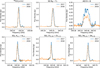 |
Fig. A.1 Comparison of observations acquired in 2017 and 2018. The observations from 2017 were convolved to the same spatial resolution as those from 2018 and the emission was computed using a circular aperture centered on the continuum peak and with diameter equal to 0″.4. |
Appendix B SO and SO2 abundance profiles
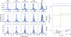 |
Fig. B.1 Predicted SO and SO2 line emission (left panels) considering different abundance profiles (right panel) and the density, temperature, and velocity distributions presented in Table 3. The line emission is shown with the same line color and style as the corresponding abundance profile. |
Appendix C Adopted partition functions and transitions constants
The energy of the upper levels and the Einstein-A coefficients were obtained from the Cologne Database for Molecular Spectroscopy (CDMS) or from the ExoMol database. When the partition functions listed in CDMS did not extend to high-enough temperatures (∼ 1000 K), we retrieved the partition function and the transition parameters from the ExoMol database. Care has to be taken that the same levels are taken into account in the partition function and on the calculation of the level populations (for instance, whether hyperfine splitting was accounted for or not).
For SO and SO2, we retrieved the transition properties and the partition function provided by Brady et al. (2024) and Underwood et al. (2016) through the ExoMol database.
For AlO, the transition properties and the partition function listed in the CDMS were used, with data from Törring & Herrmann (1989); Yamada et al. (1990); Goto et al. (1994) and Patrascu et al. (2015).
For PO, we obtained the transition properties and the partition function provided by Prajapat et al. (2017) through the ExoMol database.
For AlF, we used the transition properties and the partition function listed in the CDMS, with data compiled from Wyse et al. (1970); Hoeft et al. (1970); Maki & Lovas (1982); Hedderich & Bernath (1992) and Yousefi & Bernath (2018).
Appendix D Line emission, optical depth, and abundance maps
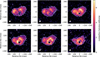 |
Fig. D.1 SO2 line emission maps. The panels show lines JKa,Kc = 4(3,1) - 3(2,2) (top left), 21(2,2q) - 21(1,21) (top middle), 34(3,31) - 34(2,32) (top right), 36(5,31) - 36(4,32) (bottom left), 40(4,36) - 40(3,37) (bottom middle), and 44(5,39) - 44(4,40) (bottom right). |
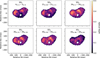 |
Fig. D.3 SO2 optical depth maps. The panels show lines JKa,Kc = 4(3,1) - 3(2,2) (top left), 21(2,20) - 21(1,21) (top middle), 34(3,31) - 34(2,32) (top right), 36(5,3i) - 36(4,32) (bottom left), 40(4,36) - 40(3,37) (bottom middle), and 44(5,39) - 44(4,40) (bottom right). |
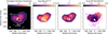 |
Fig. D.3 Maps of SO JK = 88 - 77 line emission (left), column density (middle left), averaged line optical depth (middle right), and abundance (right). |
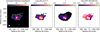 |
Fig. D.4 Maps of AlF J = 10 - 9 line emission (left), column density (middle left), averaged line optical depth (middle right), and abundance (right). |
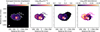 |
Fig. D.5 Maps of AlO N = 9 - 8 line emission (left), column density (middle left), averaged line optical depth (middle right), and abundance (right). |
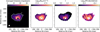 |
Fig. D.6 Maps of PO 2Π3/2 J, F = 8, 8 - 7,7 line emission (left), column density (middle left), averaged line optical depth (middle right), and abundance (right). |
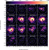 |
Fig. D.7 Channel maps of 13CO J = 3 - 2 emission. The white dashed circles with radii 40, 100, and 200 mas indicate the region from where spectra were extracted to be compared to the radiative transfer models. |
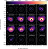 |
Fig. D.8 Channel maps of 13CO J = 3 - 2 emission from the radiative transfer model. The white dashed circles with radii 40, 100, and 200 mas indicate the region from where spectra were extracted to be compared to the radiative transfer models. |
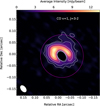 |
Fig. D.9 Observed map of CO v = 1, J = 3 - 2 emission. The white contours mark emission at 3, 5, 10, and 20 times the value of the root mean square noise in the image (0.45 mJy/beam). The magenta circle indicates the size of the inner high-density region in the radiative transfer models. |
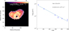 |
Fig. D.10 Example of population diagram obtained from a typical pixel. The left panel shows the SO2 column density map (also shown in Fig. 4) and the right panel shows the population diagram constructed using the line emission extracted from the selected pixel (indicated by the black square in the left panel). |
All Tables
Stellar pulsation phase at the time of the ZIMPOL observations and spatial resolution in the obtained images.
All Figures
|
Fig. 1 Images of the polarization degree (color map) toward Mira at different epochs in filters CntHa for all epochs except for 2017, which was observed with filter NR. The approximate pulsation phases (φ) of Mira A at the times of the observations are given above each panel. The white contours show the total intensity emission from Mira A at 20%, 40%, and 80% of the peak value. The red dots mark the position of the companion in the total intensity images, while the gray dots in the bottom right panel indicate the approximate position of the companion in previous epochs. The straight line used to determine the reference point on the NE lobe is shown in the upper middle panel. The 3σ contour of the SO JK = 88 - 77 emission in 2017 November (shown in Fig. 2) is marked by the magenta line in comparison to the polarized-light map at the same epoch. The gray ellipse in the bottom right corner of each panel indicates the full width at half maximum of the point spread function in the obtained images. |
| In the text | |
|
Fig. 2 Moment-zero maps of the emission in the SO JK = 88–77 line observed in 2017 November 9 and 2023 July 6 and 14. The approximate pulsation phases (φ) of Mira A at the times of the observations are given at the top of each panel. The white contours mark where emission reaches three times the RMS noise level in each image. The straight white line in the right panel indicates the direction used to measure the size of the NW lobe in the two epochs. |
| In the text | |
|
Fig. 3 Observed distance on the plane of the sky of the reference point of the NE (maroon circles) and NW (magenta squares) lobes. The magenta solid line and blue dashed line show the fits to the observed extents of the NW and NE lobes, respectively, assuming constant expansion. The magenta dot-dashed and green dotted line shows a fit to the extent of the NW and NE lobes, respectively, assuming a ballistic trajectory for a star with 1.2 M⊙. The black intervals mark the uncertainty interval on the ejection times of the lobe to the NE based on the two models. |
| In the text | |
|
Fig. 4 Results from the SO2 populations diagram. From left to right, the panels show the obtained maps of |
| In the text | |
|
Fig. 5 Observed emission (left) and inferred optical depth (middle) of the 13CO J = 3-2 line and corresponding calculated column density of 13CO (right) assuming optically thin emission and the same excitation temperature distribution derived for SO2. The dashed white circle in the middle panel marks the 60 mas radius inside of which the derived column densities are not reliable because of high optical depths. The white and magenta contours in the left and right panels, respectively, mark emission equal to three times the RMS noise level. |
| In the text | |
|
Fig. 6 Schematic view of the model with the different regions indicated. This view is a cut through the plane defined by the two major axes of the ellipses (main plane of the model). For the ray-tracing, the model is rotated about the major axis of the smaller lobe by an angle of 20°. In this way, the larger lobe is inclined toward the observer to produce the observed blueshifted emission. |
| In the text | |
|
Fig. 7 Moment-zero map of the 13CO J = 3-2 line of the best-fitting model (color map) compared to the moment zero of the observed line (white contours at levels of 3, 5, 10, and 20 times the RMS noise). The line emission and physical structure of the same model are shown in Figs. 8 and 9, respectively. |
| In the text | |
|
Fig. 8 Observed lines extracted from three different apertures (blue histograms) compared to the results from the radiative transfer model (dashed black lines) summarized in Table 3. A systemic velocity of 47 km s−1 was added to the model. |
| In the text | |
|
Fig. 9 Physical parameters of the radiative transfer model (yellow line) summarized in Table 3 and with fits to the observations shown in Fig. 8. The dashed red line shows the lower density in the NE lobe. The gray curve in the temperature panel shows a gray atmosphere temperature profile. The vertical light gray lines mark Rtrans. |
| In the text | |
|
Fig. 10 Redshifted emission excess observed in the SO2 JKa,Kc = 212, 20−211, 21 line. The red circle represents the stellar disk observed in the continuum emission. The white contour marks emission above three times the RMS noise level. |
| In the text | |
|
Fig. A.1 Comparison of observations acquired in 2017 and 2018. The observations from 2017 were convolved to the same spatial resolution as those from 2018 and the emission was computed using a circular aperture centered on the continuum peak and with diameter equal to 0″.4. |
| In the text | |
|
Fig. B.1 Predicted SO and SO2 line emission (left panels) considering different abundance profiles (right panel) and the density, temperature, and velocity distributions presented in Table 3. The line emission is shown with the same line color and style as the corresponding abundance profile. |
| In the text | |
|
Fig. D.1 SO2 line emission maps. The panels show lines JKa,Kc = 4(3,1) - 3(2,2) (top left), 21(2,2q) - 21(1,21) (top middle), 34(3,31) - 34(2,32) (top right), 36(5,31) - 36(4,32) (bottom left), 40(4,36) - 40(3,37) (bottom middle), and 44(5,39) - 44(4,40) (bottom right). |
| In the text | |
|
Fig. D.3 SO2 optical depth maps. The panels show lines JKa,Kc = 4(3,1) - 3(2,2) (top left), 21(2,20) - 21(1,21) (top middle), 34(3,31) - 34(2,32) (top right), 36(5,3i) - 36(4,32) (bottom left), 40(4,36) - 40(3,37) (bottom middle), and 44(5,39) - 44(4,40) (bottom right). |
| In the text | |
|
Fig. D.3 Maps of SO JK = 88 - 77 line emission (left), column density (middle left), averaged line optical depth (middle right), and abundance (right). |
| In the text | |
|
Fig. D.4 Maps of AlF J = 10 - 9 line emission (left), column density (middle left), averaged line optical depth (middle right), and abundance (right). |
| In the text | |
|
Fig. D.5 Maps of AlO N = 9 - 8 line emission (left), column density (middle left), averaged line optical depth (middle right), and abundance (right). |
| In the text | |
|
Fig. D.6 Maps of PO 2Π3/2 J, F = 8, 8 - 7,7 line emission (left), column density (middle left), averaged line optical depth (middle right), and abundance (right). |
| In the text | |
|
Fig. D.7 Channel maps of 13CO J = 3 - 2 emission. The white dashed circles with radii 40, 100, and 200 mas indicate the region from where spectra were extracted to be compared to the radiative transfer models. |
| In the text | |
|
Fig. D.8 Channel maps of 13CO J = 3 - 2 emission from the radiative transfer model. The white dashed circles with radii 40, 100, and 200 mas indicate the region from where spectra were extracted to be compared to the radiative transfer models. |
| In the text | |
|
Fig. D.9 Observed map of CO v = 1, J = 3 - 2 emission. The white contours mark emission at 3, 5, 10, and 20 times the value of the root mean square noise in the image (0.45 mJy/beam). The magenta circle indicates the size of the inner high-density region in the radiative transfer models. |
| In the text | |
|
Fig. D.10 Example of population diagram obtained from a typical pixel. The left panel shows the SO2 column density map (also shown in Fig. 4) and the right panel shows the population diagram constructed using the line emission extracted from the selected pixel (indicated by the black square in the left panel). |
| In the text | |
Current usage metrics show cumulative count of Article Views (full-text article views including HTML views, PDF and ePub downloads, according to the available data) and Abstracts Views on Vision4Press platform.
Data correspond to usage on the plateform after 2015. The current usage metrics is available 48-96 hours after online publication and is updated daily on week days.
Initial download of the metrics may take a while.