| Issue |
A&A
Volume 707, March 2026
|
|
|---|---|---|
| Article Number | A58 | |
| Number of page(s) | 16 | |
| Section | Stellar structure and evolution | |
| DOI | https://doi.org/10.1051/0004-6361/202557724 | |
| Published online | 26 February 2026 | |
RR Lyrae stars with variable mean magnitudes
1
Nicolaus Copernicus Astronomica Center Bartycka 18 00-629 Warsaw, Poland
2
Konkoly Observatory, HUN-REN Research Centre for Astronomy and Earth Sciences Konkoly-Thege Miklós út 15-17 Budapest H-1121, Hungary
3
Instituto de Astrofísica, Pontificia Universidad Católica de Chile Av. Vicuña Mackenna 4860 Macul 7820436 Santiago, Chile
4
Millenium Institute of Astrophysics Nuncio Monseñor Sotero Sanz 100 Providencia Santiago, Chile
5
Departmento de Astronomía, Universidad de Concepción Casilla 160-C Concepción, Chile
6
Astronomical Observatory, University of Warsaw Al. Ujazdowskie 4 Warsaw 00-478, Poland
7
Korea Astronomy and Space Science Institute Daejeon 34055, Republic of Korea
★ Corresponding author: This email address is being protected from spambots. You need JavaScript enabled to view it.
Received:
16
October
2025
Accepted:
14
December
2025
Abstract
Context. A number of RR Lyrae stars exhibit variable mean magnitudes in the OGLE survey light curves of the Galactic bulge. Hitherto, this phenomenon has not been studied, as it was generally assumed to be related to photometric issues.
Aims. We investigate whether the mean magnitude variability of RR Lyrae variables is due to genuine astrophysical phenomena.
Methods. We used the extended, and in many cases overlapping, light curves from multiple microlensing surveys to study RR Lyrae stars with apparent mean-magnitude variations. A modified Fourier-series based fitting method is introduced to analyze the light curves showing mean-magnitude variations. Data from infrared surveys were also used to construct spectral energy distributions (SEDs).
Results. Presented here are 72 stars where the mean-magnitude variations are most probably of genuine astrophysical origin, rather than the result of photometric problems. The ratio of variation between the V and I bands is compatible with variable extinction by dust in most cases, but no infrared excess is detected in the SEDs. The occurrence rate of the phenomenon, after correcting for selection effects, is ∼0.9% among RR Lyrae variables in the OGLE bulge fields.
Key words: circumstellar matter / stars: variables: RR Lyrae / dust / extinction / Galaxy: bulge
© The Authors 2026
 Open Access article, published by EDP Sciences, under the terms of the Creative Commons Attribution License (https://creativecommons.org/licenses/by/4.0), which permits unrestricted use, distribution, and reproduction in any medium, provided the original work is properly cited.
This article is published in open access under the Subscribe to Open model. This email address is being protected from spambots. You need JavaScript enabled to view it. to support open access publication.
1. Introduction
RR Lyrae (RRL) variable stars are widely used as tracers and probes of old stellar populations, in both the Milky Way (Hernitschek et al. 2017; Prudil et al. 2019; Kunder et al. 2020; Wang et al. 2022; Cabrera Garcia et al. 2024) and other galaxies of the Local Group (Mateo et al. 1995; Clementini et al. 2003; Musella et al. 2012; Contreras Ramos et al. 2013; Jacyszyn-Dobrzeniecka et al. 2017; Karczmarek et al. 2017; Tanakul & Sarajedini 2018; Savino et al. 2022). As part of its regular survey observations, the Optical Gravitational Lensing Experiment (OGLE; Udalski et al. 2015) monitors the Galactic bulge at a high cadence, incidentally providing light curves for tens of thousands of RRL stars in this region (Soszyński et al. 2014). We recently undertook a search for RRL stars in binary systems using this treasure trove of data (Hajdu et al. 2021), using the light-travel time effect (LTTE; Irwin 1952). During our search, we also visually inspected the light curves of each of the analyzed ∼27 000 fundamental-mode RRL stars (RRab subclass). We noticed that some of them exhibit long-term variability in their mean brightness. In previous studies, these were either ignored or assumed to be due to photometric trends and were subsequently removed (Prudil et al. 2017; Netzel et al. 2018).
Due to the importance of RRL variables as stellar population tracers and standard candles for distance determination, it is crucial to investigate possible sources of bias affecting their properties. Therefore, we decided to perform a systematic revision of mean-magnitude changes in the same sample of stars using photometry from OGLE as well as other surveys. The results are presented in this article, which is organized as follows: Section 2 presents the utilized data, Section 3 describes the light curve analysis procedure. In Section 4 we discuss the sample properties, and finally in Section 5 we put the results in context and hypothesize on the possible origin of the mean-magnitude changes.
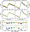 |
Fig. 1. Summary plot for one of the analyzed stars. Panel a: original OGLE I-band light curve folded with the period of pulsation, with the corresponding Fourier fit overlaid. Panel b: same as (a), but with the long-term changes removed. Panel c: same as (a), but for the V-band data. Panel d: same as (b), but for the V-band data. Panel e: I-band data after subtraction of the Fourier light-curve model. The orange dots and lines show the fit of the long-term changes in brightness. Panel f: same as (e), but for the V-band light curve. All light-curve points are colored according to the estimated mean-magnitude values during the observations, with lighter and darker points corresponding to brighter and fainter epochs, respectively. Above the panels, the OGLE ID, pulsation period, amplitude (ΔIDR(I)), and amplitude ratio (rI, V = A(I)/A(V)) of the mean-magnitude changes are given. The complete set of summary plots is available as online material. (see Data availability paragraph). |
2. Utilized data
The main analysis was performed using the Johnson-Kron-Cousins V and I-band time series photometric measurements of OGLE’s Galactic bulge RRL sample (Soszyński et al. 2014), obtained during the survey’s fourth phase (OGLE-IV; Udalski et al. 2015). The currently public data were extended for the analyzed objects with unpublished data from the 2018 and 2019 observing seasons. Furthermore, we also extracted from the OGLE internal catalogs the light curves of stars within 10 arc seconds of RRL stars on our short list of candidates and used those to assess possible photometric contaminations (see Section 3). Light curves from the Massive Compact Halo Object (MACHO; Alcock et al. 1993), Expérience pour la Recherche d’Objets Sombres phase 2 (EROS-2; Tisserand et al. 2008), Korea Microlensing Telescope Network (KMTNet; Kim et al. 2016), Microlensing Observations in Astrophysics (MOA; Sako et al. 2008) surveys, and the third phase of the OGLE project (OGLE-III; Soszyński et al. 2011) were also revised during the analysis to search for independent evidence of mean-magnitude changes similar to those detected in the OGLE-IV photometry. Additional details about the utilized optical photometry, including the transformation of KMTNet and MOA differential fluxes onto a magnitude scale, are given in Appendix A.
We also utilized proper motions taken from the Gaia Data Release 3 catalog (DR3; Gaia Collaboration 2023). However, in the dense environment of the bulge, the catalog is incomplete and proper motions have relatively large errors for the highly reddened RRL variables. Furthermore, formal errors in the Gaia DR3 catalog might be underestimated by a factor of up to 4 in the most dense bulge fields (Luna et al. 2023). Therefore, for our final sample, we replaced the Gaia DR3 proper motions for RRab stars on our list with the values from the prerelease version of the OGLE-Uranus proper motion catalog (Udalski et al., in prep.). The OGLE-Uranus catalog has on average smaller formal errors, especially for the most reddened (V − I > 2) variables.
During the construction of spectral energy distributions (SEDs; Section 4.4), we also used the near-infrared (near-IR) JHKS light curves obtained by the Vista variables in the Vía Láctea (VVV; Minniti et al. 2010) survey, as well as the mid-infrared (mid-IR) flux measurements provided by the Galactic Legacy Mid-Plane Survey Extraordinaire (GLIMPSE; Churchwell et al. 2009) family of surveys.
Analysis summary of the final sample of RR Lyrae stars with mean-magnitude changes.
3. Search for RRL variables with changing mean-magnitudes
During our initial search for mean-magnitude changes in RRL stars, we visually inspected the OGLE-IV light curves from the 2010 to 2017 observing seasons for the same sample of RRL stars as in our search for binary RRL (Hajdu et al. 2021). A total of ∼250 stars were selected for this long list of candidates, only omitting stars where it was obvious from the light curves that the mean-magnitude changes were caused by photometric problems (e.g., the mean magnitude showed a clear correlation with the pulsation amplitude).
The RRL light curves in the long-term OGLE photometry can suffer from various biases. They can blend together with other variable stars, might be affected by light scattered within the camera from very bright stars in the field, or trends can arise from problems with the image subtraction photometry caused by their changing position on the sky over time (for stars with high proper motions). Therefore, the OGLE-IV I- and V-band light curves were inspected for any suspicious trends associated with these effects. Time series data from other surveys were also revised during this analysis, and a few stars with completely stable light curves in these were also removed. A particularly notable group of stars in the field of the globular cluster NGC 6441 was removed altogether, as their light curves all showed the same general trend and a common break point in their mean-magnitude behavior in the OGLE-IV light curves, whereas the OGLE-III light curves were completely stable. In this case, we suspect that the foreground star G Sco (V ∼ 3.2 mag) is the source of the contamination in the OGLE-IV data.
All in all, more than half of the stars from the initial long list were removed in this step, resulting in a short list of ∼100 variables. These were further revised, and their light curves were fit multiple times using both traditional and modified Fourier series that allow for changing mean magnitudes (see Appendix B for a description of the latter method). Figure 1 shows a typical example for the analysis with mean-magnitude changes. The solutions were iterated and analyzed to identify and remove the last few dubious cases. The light curves of all sources detected by OGLE-IV within 10 arcseconds of these RRL were also extracted and analyzed. The light curves of a handful of RRL variables were clearly contaminated by other nearby variable stars, and were therefore removed from the list. Furthermore, we required the OGLE-IV I and V band light curves to show the same general trends in the mean magnitudes of the variables. To this end, we calculated the difference in the Akaike information criterion (AIC; Akaike 1974) between the traditional Fourier series and the mean-magnitude-changing Fourier series solutions in the V band (ΔAIC). A few stars with ΔAIC less than 20 were removed at this step1. Unfortunately, some good candidates have too few V-band detections or were not detected at all by OGLE-IV in the V band (due to high extinction), and these stars were also removed. Other candidates display annual trends in their photometry, which are clearly visible in the changes of the mean magnitudes. Variables where the only clear reason for the mean-magnitude changes was these annual trends were removed from the sample. In contrast, we chose to retain variables where the long-term mean-magnitude changes were completely explained by our light-curve modeling for both bands and confirmed by other photometric sources, despite their light curves also showing annual trends (e.g., OGLE-BLG-RRLYR-01591, -08752, and -11931).
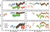 |
Fig. 2. Comparison of RRL mean-magnitude changes between different surveys. Each panel shows the OGLE-IV, OGLE-III, MACHO, EROS-2, MOA, and KMTNet light curves (black, blue, brown, purple, green, and red dots, respectively; see their descriptions in Appendix A) after subtraction of (separate) Fourier light-curve models for each dataset. Light curves are offset by arbitrary amounts for clarity. The overlaid orange dots and lines show the mean-magnitude change modeling according to the light-curve fits, similarly to panel (e) of Fig. 1. Above the panels, the OGLE ID, the pulsation period, the amplitude of the mean-magnitude changes, and the measured amplitude ratio rI, V = A(I)/A(V) are given for the corresponding RRL, based on the OGLE-IV data. |
4. Properties of the final sample
After the final revision of the short list of candidates, we were left with 71 RRab stars, all displaying variable mean magnitudes in both their I- and V-band photometry. While we have not yet performed a dedicated search among first-overtone RRL stars (RRc subclass) for this effect, one such variable, OGLE-BLG-RRLYR-34373, has a remark on its variable mean magnitude in the OGLE bulge RRL catalog (Soszyński et al. 2014). After analyzing its light curve, we concluded that it shows the same phenomenon as the RRab variables; therefore, it was added to the sample considered here, for a total of 72 RRL stars on this final list. The properties of these variables are summarized in Table 1. We note that during the fitting process, a few outlying light curve points were removed manually for most variables, and the corresponding number of points is also given in the table. The amplitude of the mean-magnitude changes is quantified by the inter-decile range in the I-band (ΔIDR(I)) calculated on the mean magnitudes (m0, z) at the times of each adopted break point (tz) of the modified Fourier fit, as described in Appendix B. Furthermore, the amplitude ratio of the mean-magnitude changes, defined as rI, V = A(I)/A(V), is also listed, alongside the Fourier orders selected by our method in the I and V bands, and the difference in AIC values calculated for the V-band solutions. Finally, the appearance of the mean-magnitude changes in the OGLE-IV light curves is classified into four categories: (1) mostly monotonic increase or decrease; (2) both increasing and decreasing intervals at different times; (3) quasiperiodic appearance; (4) exhibiting complex variations.
The long-term behavior of the mean-magnitude changes differs between stars, as shown in Figure 2. The OGLE-IV data (black dots) show that the majority of variables display the smoothest mean-magnitude behavior near maximum brightness. In contrast, stars with large amplitude mean-magnitude variations typically display sharp, asymmetric drops, mostly in their dimmer light-curve phases, although some lower-amplitude variables can behave similarly (see the bottom-right and top-right panels of Figure 2 for respective examples). Light curves from surveys overlapping with OGLE observations show an excellent agreement in the shapes of the mean-magnitude behavior for the majority of cases. As these data are independent of each other, this eliminates the possibility that the observed mean-magnitude changes are caused by problems with the OGLE-IV photometry. Earlier surveys usually have lower photometric accuracy and fewer data points, but they also show the same type of light-curve behavior as more recent data. In a few cases, quasiperiodic patterns also appear on long timescales. OGLE-BLG-RRLYR-12793 (top-right panel of Figure 2) shows a possibly periodic (or quasiperiodic) behavior with a tentative period of ∼2500 d or ∼5000 d; OGLE-BLG-RRLYR-34373 (bottom-right panel) similarly shows a possible periodicity on a timescale of ∼4000 d or ∼8000 d. Information on the presence of detectable mean-magnitude changes in the MACHO, EROS-2, OGLE-III, MOA, and KMTNet light curves is given in Appendix C for all stars on our final list.
We note that while our fitting works well for most stars, some (i.e., OGLE-BLG-RRLYR-02401, -04444, and -10084) show minor deviations in the mean-magnitude changes in the V band, when compared to the I band. These differences may arise from unaccounted-for biases in the photometry or, alternatively, reflect real differences between the behavior of the phenomenon between the V and I bands.
4.1. Light-curve properties
The light-curve shapes of RRL stars provide information about their physical parameters (Jurcsik & Kovács 1996; Bellinger et al. 2020), which in turn inform us about their host stellar populations. The top and middle panels of Figure 3 compare the distribution of pulsation amplitudes and the light-curve shape parameter ϕ31 (Simon & Teays 1982) of our sample to that of the OGLE survey toward the Galactic bulge. About half of our sample lie on top of the main ridge of the dominant bulge RRL population (Pietrukowicz et al. 2020) on both panels (the exact number is between 30 and 40, depending on its assumed width). The remainder have light-curve parameters mostly typical of RRL stars in Oosterhoff II type systems (Catelan & Smith 2015), suggesting that they have lower metallicities on average. Some might be halo interlopers, which make up between 8 and 25 percent (Prudil et al. 2019; Kunder et al. 2020) of the RRL variables observed in the Galactic bulge.
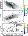 |
Fig. 3. Top panel: period–amplitude (Bailey) diagram of the OGLE bulge RRab sample (gray 2D histogram, shown on a logarithmic scale) and the mean-magnitude-changing RRL variables with circles colored according to the measured I-band mean-magnitude changes. Middle panel: distribution of epoch-independent phase differences (ϕ31) of the RRab stars. Bottom panel: dependency of the amplitude ratio rI, V on the amplitude of the I-band mean-magnitude changes. RRab stars are marked with circles and are colored according to their pulsation periods, while the single RRc star is marked with a black square. The horizontal dashed lines indicate the expected extinction ratios for different RV values of the standard interstellar extinction law (Cardelli et al. 1989). |
The bottom panel of Figure 3 compares the amplitude ratio of the mean-magnitude changes in the two bands (I, V) and its total amplitude in the I band (ΔIDR(I)). If the changes are caused by intervening dust, then the amplitude ratio can be interpreted as an extinction ratio between the two bands. These are compatible with dust composed of submillimeter-sized particles, as shown by the comparison to the standard interstellar extinction curve (Cardelli et al. 1989). However, we do note that a few RRL variables have amplitude ratios more in line with a nearly flat “gray” extinction, which can be caused by substantially larger average grain sizes (Weingartner & Draine 2001). Alternatively, if the changes are interpreted as intrinsic variations of RRL stars, the amplitude ratios are also comparable to variability caused by stellar spots in red giants. Specifically, using the OGLE sample of rotating variables toward the Galactic bulge (Iwanek et al. 2024), we calculated tenth, median, and 90th percentile values of the amplitude ratio AI/AV of 0.31, 0.52, and 0.79, respectively, for stars with Prot > 20 d.
One RRL star showing mean-magnitude changes, OGLE-BLG-RRLYR-09197, experienced a single eclipse-like fading during the third phase of the OGLE project (Soszyński et al. 2011). The observing season of the event is marked with vertical dashed lines on the left-middle panel of Figure 2. This event is by far the sharpest drop in brightness detected in any of the stars presented here. Figure 4 shows the data from 2008, after the removal of both the pulsation and the long-term mean-magnitude change signals. While few light curve points from OGLE cover this event, the contemporaneous MOA data unambiguously confirms it2. This asymmetric event lasted ∼12 days, with a slow ingress, quick egress, and a local maximum near the center of the event. This shape is reminiscent of eclipses produced by objects surrounded by rings and/or disks, such as:
-
the Be star surrounded by at least two circumstellar disks, eclipsing the peculiar W Virginis variable OGLE-LMC-T2CEP-211 (Pilecki et al. 2018);
-
the disk-shrouded, low-mass companion of a B star in the eclipsing binary OGLE-LMC-ECL-11893 (Scott et al. 2014);
-
the dark disk surrounding the invisible companion of a Be star in the binary EE Cep (Gałan et al. 2012);
-
the occulting dark disk in the binary ELHC 10 (Garrido et al. 2016).
The eclipse event shown in Figure 4 makes OGLE-BLG-RRLYR-09197 the best candidate for an RRL variable in an eclipsing binary system. However, no similar eclipse has been observed before or after this singular event, suggesting a very long orbital period.
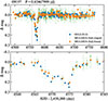 |
Fig. 4. Eclipse-like event of OGLE-BLG-RRLYR-09197. Top: residual light curve of the 2008 observational season. Both pulsation and long-term mean-magnitude changes are subtracted. OGLE and MOA observations are shown with blue and green dots, respectively. For clarity, daily average magnitudes for the MOA data are also shown with orange points. Bottom: same as the top panel, but showing the event between the limits marked by vertical dashed gray lines. |
4.2. The incidence rate
Estimating the true incidence rate of the mean-magnitude changes in RRL stars is complicated by the fact that the sampling of the OGLE light curves strongly depends on the star’s position in the sky. In general, OGLE-IV fields with high stellar densities in the Galactic bulge regions are observed more frequently, due to the higher occurrence rate of microlensing events (see Fig. 15 in Udalski et al. 2015).
Figure 5 shows the distribution of I-band magnitudes as a function of the number of available I-band data points (during the OGLE-IV 2010-2017 seasons) of the analyzed sample of stars. Stars in our sample are all relatively bright with I ≲ 17.95 mag and have at least 680 data points. There are a total of 11 449 stars in the initial sample if we adopt I < 18.1 mag and NI > 660 as the absolute detection limits. Then, an initial estimate for the incidence rate of the mean-magnitude changes would be 71/11 449 ∼ 0.6%.
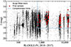 |
Fig. 5. Distribution of the available I-band data points and mean magnitudes in the OGLE survey for RRab stars (black points). The stars in our final sample are marked with red circles. The dashed blue lines denote the region used to calculate the incidence rate of the mean-magnitude changing effect in RRab stars. |
An additional complication for detecting the mean-magnitude changes is the presence of the Blazhko effect. The Blazhko effect modulates the light curve shapes and amplitudes in a high fraction of RR Lyrae stars with periods of a few days to multiple years, and with amplitudes ranging from millimagnitudes to multiple tenths of a magnitude (Smolec 2016). In our experience, the detection of mean-magnitude changes, which have typical amplitudes below 0.1 mag in the I band (see the bottom panel of Figure 3), is significantly complicated by its presence. Assuming that these two effects operate independently of one another, this can be roughly corrected for by taking into account the fraction of Blazhko stars in the sample and the occurrence rate of the Blazhko effect, similarly to our investigation of RRL binarity with the LTTE (Hajdu et al. 2021). In the final sample, there are only ten Blazhko stars (14%; see Appendix C). The incidence rate of the Blazhko effect in the OGLE Galactic bulge RRab sample is at least 40% (Prudil & Skarka 2017). Given the 61 RRab stars in the final sample with no Blazhko effect detected, we would expect to detect ∼40 stars showing the Blazhko effect and mean-magnitude variations at the same time (instead of ten), for a total of ∼101 detections. Taking into account the data quantity and brightness cuts, this increases the incidence rate to ∼0.9%, which can be adopted as a lower limit for the incidence rate for RRab stars presenting real changes in their mean magnitudes. Given this relatively low occurrence rate, we surmise that the mean-magnitude changes reported here have a negligible effect on the utility of RR Lyrae stars as standard candles.
4.3. Sky distribution, color-magnitude diagram, and proper motions
The distribution of stars in our final sample might give us additional hints about the cause of the mean-magnitude changes. The top panels of Figure 6 show the sky distribution of the sample reported here (red dots), compared to the distribution of RRL stars in the OGLE-IV sample that pass the detectability limits (I < 18.1 mag and NI > 660) adopted in Section 4.2. In the top-left panel, the RRL variables are colored according to their V − I colors (as a proxy for the reddening), while in the top-right panel they are colored according to the number of available OGLE-IV I-band data points. In the southern bulge fields, the number density of both our sample and that of the RRab variables in general steadily increases toward the Galactic plane, and this increase stops only when the extinction pushes the RRL magnitudes beyond our adopted cutoff of 18.1 mag. The top-right panel also clearly shows that stars from our sample are preferentially located in regions with the largest amount of photometric points.
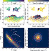 |
Fig. 6. Properties of the 71 RRab stars in our sample (red dots) vs. stars used for incidence rate calculation (see Figure 5). Top left: distribution of RRab stars in Galactic coordinates. Colors correspond to the V − I color of each RRab star. Top right: same as top left, but with the colors corresponding to the number of available I-band data points. Bottom left: I vs. V − I color-magnitude diagram of the RRab stars. The white arrow denotes the reddening vector for 1 magnitude of color excess for RV = 3.1 (Cardelli et al. 1989). Bottom right: proper motion distribution of the sample. The dashed white ellipse denotes the two standard deviation distances from the sample median. |
The bottom-left panel of Figure 6 shows the color-magnitude diagram of the final sample, while the OGLE-IV sample (after applying the detectability cuts) is represented by the linearly scaled 2D histogram. Curiously, the distribution of our sample does not follow that of the general bulge sample, with our stars being preferentially closer, and in some cases farther, than the Galactic bulge. Two stars in our sample (OGLE-BLG-RRLYR-02401 and -06019, marked with arrows) are apparently closer than 4 kpc, i.e., less than half the distance to the Galactic center. The difference between the two samples is further corroborated by the distributions of proper motions shown on the bottom-right panel. The peak of the distribution of the complete sample (shown again by the 2D histogram scaled linearly) corresponds to the mean motion of bulge stars. The dashed white ellipse shows the 2σ distance from the sample median (where the standard deviations were measured using the robust median absolute deviations). As seen, a sizable fraction of stars are quite far from the median of the total sample. To quantify this, only 30% and 69% of the stars of the mean-magnitude-changing RRL stars reported here are within 1σ and 2σ distance from the sample median, respectively (compared to the expected 39% and 86%, respectively). Therefore, the bottom panels of Figure 3 hint at a difference between the general (bulge-dominated; Prudil et al. 2019; Kunder et al. 2020) RRL sample and the RRL variables showing mean-magnitude changes, similarly to the top and middle panels of Figure 3, showing the light-curve parameters of the RRab stars.
To correctly assign every RRL of our final sample to its parent stellar population (i.e., Galactic bulge, halo, or disk), a complete dynamical analysis is necessary. Unfortunately, most of these stars currently lack a radial velocity measurement, preventing us from performing said analysis. Furthermore, due to the mean-magnitude changes themselves, a judicious application of period–luminosity–metallicity relationships will be necessary to correctly estimate their distances.
4.4. Transiting mass estimate and spectral energy distributions
Under the assumption that the mean-magnitude changes are caused by variable extinction due to circumstellar dust, a minimum mass of the material transiting the disk of the RRL stars can be estimated. We did so by adopting an orbital distance and geometry, as well as a specific dust mass-to-extinction ratio (see details in Appendix D). This led to lower limits of ∼1.3 × 10¹⁸ kg, ∼6.7 × 10¹⁷ kg, and ∼1.1 × 10¹⁸ kg, for the RRL variables with the highest inferred extinction amounts, namely, OGLE-BLG-RRLYR-05572, -11061, and -34373, shown in the top-left, bottom-left, and bottom-right panels of Fig. 2, respectively. For comparison, the mass of a 90 km diameter asteroid with a density of ∼3 g cm−3 (typical of S-type asteroids; Vernazza et al. 2021) is ∼1.1 × 10¹⁸ kg, i.e., the same order of magnitude as the inferred dust masses. To put this number into context, this is ∼5.4 million times less than the mass of the Earth.
Circumstellar material can be detected around stars by the infrared excess in their SEDs, with its strength and shape depending on the mass, temperature, geometry, and chemical properties of the dust present. As these features are generally the strongest in the mid- and far-infrared wavelengths, we searched all infrared archives for the longest-wavelength observations available to include in our SEDs. Unfortunately, the large distance, high backgrounds, and crowding resulted in only three stars being detected in the 8 μm band in the GLIMPSE surveys by the Spitzer space telescope (Werner et al. 2004). None of our stars were detected by surveys at longer wavelengths.
We constructed our SEDs for the three stars detected in the 8 μm band in the GLIMPSE surveys. The optical and near-IR parts of the observed SEDs were constructed using the pulsation-averaged magnitudes of the stars. In the Johnson-Kron-Cousins V and I bands, the values provided by the OGLE-IV catalog were adopted. In the near-IR JHKS bands, the VVV survey light curves were fit using a principal component-based fitting method (Hajdu et al. 2018), after correcting the original VVV light curves for known issues affecting their photometric zero points (Hajdu et al. 2020). The VIJHKS magnitudes were converted to fluxes using photometric zero points provided by the SVO Filter Profile Service (Rodrigo & Solano 2020), and 5% measurement uncertainties were assumed for all bands. For the mid-IR part of the SED, the GLIMPSE flux measurements in the four mid-IR bands were adopted alongside their quoted errors.
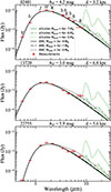 |
Fig. 7. Spectral energy distributions of RRL with 8 μm photometry available. On each panel, the measured fluxes of a star are marked with red dots. The vertical and horizontal bars mark the measurement uncertainties and the effective widths of the photometric bands, respectively. The black and green curves correspond to DUSTY models with circumstellar envelopes made of amorphous carbon and silicate dust, respectively. The solid, dash-dotted, and dotted lines show progressively higher amounts of dust. Above each panel, the OGLE ID, the adopted values of V-band extinction, and distance are given. The locations of these three stars are marked by arrows on the color-magnitude diagram of the final sample (bottom-left panel of Fig. 2). |
The expected infrared excess was modeled using the radiative transfer code DUSTY (Ivezić et al. 1999). For the stellar parameters, we adopted typical values for RRL variables of L = 50 L⊙, R = 5.3 R⊙, and Teff = 6200 K (similar to those of the prototype of the class; Kolenberg et al. 2010), and the stellar SED was approximated as a blackbody. The models were constructed for two different dust chemical compositions, one typical for olivine with a 40–60% magnesium-to-iron ratio, and one for amorphous carbon (Hanner 1988). The grains were assumed to be spherical and follow a standard size distribution (Mathis et al. 1977). The gas-to-dust mass ratio was kept at 140 for all models. The models were calculated assuming spherical symmetry, with the internal shell temperature set to 800 K, resulting in an internal shell radius of ∼4 AU for all models. The thickness of the shell was set to be 10% of the internal shell radius. For both compositions, a set of models was calculated by increasing the amount of I-band extinction from the shell itself in increments of 10×. The total dust mass also scales with this factor between the models.
To compare the model SEDs to the flux measurements of the RRL variables, the former were reddened according to the Fitzpatrick & Massa (2007) interstellar reddening law using the extinction Python package (Barbary 2016), while the distance to the star with the simulated SED was varied simultaneously until a reasonable match was reached for the optical and near-IR fluxes. As seen in Fig. 7, our theoretical SEDs match the data well. It is also clear from the 3.6 and 4.5 μm fluxes that the observations are incompatible with dust made of large amounts of exclusively amorphous carbon particles, and that the currently available observations are insensitive to even large quantities of silicate dust (with the dotted green line showing the model corresponding to dust with ∼200× the mass than inferred for the transiting material). We assess that future observations in wavelengths longer than 8 μm might reveal the silicate emission feature. However, we also note that the detection of the 10 μm silicate emission could be obscured by the absorption of the same feature by interstellar matter (Roche & Aitken 1984), which is nontrivial to correct for, even for comparatively close stars with low extinction (Hocdé et al. 2020).
4.5. Connection to binarity
The deep eclipse event discussed in Section 4.1 raises the possibility that the observed mean-magnitude changes are caused by circumstellar matter, as in binary post-asymptotic giant branch (post-AGB) stars (Waelkens et al. 1991; Van Winckel et al. 1995). Establishing a correlation between the presence of binarity and the mean-magnitude changes might lend support to this hypothesis. Of the 71 RRab stars in our final sample, five are binary candidates detected through the LTTE signal. Two of these systems (OGLE-BLG-RRLYR-08215 and -08752) have estimated minimum companion masses (Hajdu et al. 2021) close to the expected mass of old white dwarfs (∼0.6 M⊙; Cummings et al. 2018), meaning that they could be in such a system with a coplanar circumbinary disk close to an inclination of 90 degrees. However, the other candidate companions have much lower minimum masses, which can be reconciled if their disks are in a polar configuration with respect to the orbital plane of the binary, as in the case of the post-AGB star AC Her (Martin et al. 2023).
To assess the possible connection between the binarity of RRL stars and the detected mean-magnitude changes, we can estimate the probability of finding stars showing both behaviors in their light curves simultaneously. In our previous work, we detected 87 binary candidates among RRab stars using OGLE photometry (Hajdu et al. 2021). During our analysis, one additional variable was found to possess a strong LTTE signal (see Appendix E), for a total of 88 such systems. Out of these, 86 are within the detectability limits shown in Figure 5. Assuming that the binarity and mean-magnitude changes are unrelated, the probability of randomly selecting (at least) five common stars from the two samples (the 86 binary candidates, and the 71 mean-magnitude changing RRab variables) out of 11 499 possible objects is ∼0.02%; selecting at least four is ∼0.2% and at least three is ∼1.6%. The one-tailed Z test suggests that the ∼0.02% probability indicates that the two samples are correlated at the ∼3.5σ level, which we deem significant enough to mention, but do not consider definitive proof yet. We note that detecting RRL stars in binary systems with the LTTE is a challenging task, due to the long binary periods, limited data, and the pulsation of RRL stars themselves. In the case of the mean-magnitude-changing RRL stars, photometric uncertainties are also increased by the detected variable extinction. Therefore, a more careful analysis with additional data could possibly uncover more binary candidates in the sample of stars reported here, increasing the significance of the suggested connection between the two phenomena.
5. Discussion
To our knowledge, similar variations in mean magnitudes have never been reported or predicted for RRL stars in the literature. In this section, we discuss the possible causes of the observed mean-magnitude changes in light of the properties of the final sample (Section 4).
5.1. Circumstellar and circumbinary material around RR Lyrae
Arguably the simplest explanation for the observed light curves (Figs. 1 and 2) is an RRL variable surrounded by a dusty disk that orbits and eclipses the star, causing the observed mean-magnitude changes. If the RRL star is single, then the disk is circumstellar, and the variations are caused by inhomogeneities in the disk. In contrast, if the RRL is in a binary system, surrounded by a circumbinary disk, then part of the variability may be due to periodic obscuration by the disk as the RRL star orbits the system’s center of mass.
In the circumstellar disk case, the most probable source of dust is the RRL star itself. Before evolving onto the horizontal branch (HB), where they are observed today, they previously passed through the red giant branch (RGB) phase, losing ∼0.2 M⊙ material before the helium core flash (Gratton et al. 2010; Tailo et al. 2020). At the same initial mass, age, and chemical composition, stars arriving on the zero-age HB (ZAHB) bluer than the instability strip (IS) must lose more mass on the RGB (Catelan 2009). Therefore, a higher fraction of longer-period RRL stars, some of which are expected to be over-luminous stars evolved off the blue HB, might exhibit higher fractions of detectable variable extinction from dust, if dust formed from material lost on the RGB causes the mean-magnitude changes. This possibility aligns well with the distribution of the sample of stars presented in the top and middle panels of Fig. 3. On the other hand, in this RGB mass loss scenario, we could reasonably expect the amount of dust around the star to slowly decrease once it leaves the RGB tip, with the largest amount expected around pre-ZAHB stars. If these stars pulsate as RRL variables (i.e., falling within the IS), they are expected to exhibit high negative period change rates, with the most likely value being β ∼ −0.3 d Myr−1 (Silva Aguirre et al. 2008). In our sample, only two stars have relatively high (06316, 12833; β ∼ −0.3 d Myr−1) negative period change rates, and another has a moderately high (01081; β ∼ −0.2 d Myr−1) negative period change rate, with the vast majority having close to zero or slightly positive rates. As approximately one star is expected to be in the pre-ZAHB phase for every 60 HB stars, the period changes do not support this premise strongly (Silva Aguirre et al. 2008).
Alternatively, dust in the stellar systems of RRL variables might continually form from ongoing mass loss of the RRL stars themselves. Mass loss has been observed in HB stars both redder (Dupree et al. 2009) and bluer than RRL variables (Krtička et al. 2016). Continuous mass loss of RRL variables – with rates of up to 10−9 M⊙ yr−1 in evolutionary calculations – has been invoked to explain the mass dispersion of stars on the HB (Koopmann et al. 1994), while temporary mass loss in certain evolutionary phases has been hypothesized to explain the period distribution of RRL variables in certain globular clusters (Catelan 2004). Radial pulsation periodically decreases the surface gravity, which in turn might lead to pulsation-induced mass loss (Wilson & Bowen 1984). Given the composition of the Sun (Asplund et al. 2009) scaled to a typical RRL iron abundance of [Fe/H] = −1.5, the sum of the mass fractions of the main dust-forming elements (carbon, magnesium, silicon, and iron) is ∼0.016%. At the above quoted mass loss rate of 10−9 M⊙ yr−1, an RRL star would lose ∼3.2 × 10¹⁷ kg of these elements in a year. Supposing a dust formation efficiency of 1% and a correction factor of 100 due to the non-transiting parts of the dust, this mass loss would produce the estimated amount of dust (see Section 4.4 and Appendix D) on a timescale of ∼105 yr. Therefore, taking into account the total length of the HB phase (tens of megayears; Silva Aguirre et al. 2008), this scenario might explain the amount of observed dust, even if the mass loss is episodic and relatively short-lived (Catelan 2004). However, the mass loss rate of 10−9 M⊙ yr−1 should probably be treated as an upper limit, as higher rates would lead to significant changes in the morphology of the HB, leading to disagreement between HB models and observations (Koopmann et al. 1994). Furthermore, we note that the fast winds inferred for red HB stars from chromospheric lines (Dupree et al. 2009) would probably result in low dust formation efficiency in the vicinity of the variables.
If the RRL is located in a binary system surrounded by a circumbinary disk, it is possible that the dust was formed from material lost by the RRL variable, either in the preceding RGB phase or from mass loss on the HB – similarly to the circumstellar scenario discussed above. While our knowledge of RRL binarity is very limited (Hajdu et al. 2021), presumably the most probable companions of RRL stars are low-mass (< 1 M⊙) main-sequence stars and white dwarfs. No significant mass loss can be expected from the former, while white dwarfs are known to have lost their outer layers previously during the post-AGB phase of their evolution. Post-AGB stars in binary systems tend to form massive dusty disks (van Winckel 2019), with masses of up to about 1% of the Sun (Gallardo Cava et al. 2021). Therefore, what we observe today might be leftover material from this brief phase, after which the post-AGB companion evolved into the RRL variable we observe. We can surmise that the amount of dust remaining in circumbinary orbit would mostly depend on the amount of dust formed in the post-AGB phase, the fraction that survives photo-evaporation once the post-AGB star becomes hotter before becoming a white dwarf (van Winckel 2003), and the time elapsed since. The latter can be quite short (tens of megayears) in systems where the two stars originally had very similar masses. Solar-type stars in binaries around the Sun (RRL progenitors are old solar-type stars) have relatively high twin fractions (∼14% for 2 < log P[day] < 6; Moe & Di Stefano 2017), possibly supporting this scenario. If the post-AGB (now white dwarf) star had a higher main-sequence mass, the time elapsed since the post-AGB phase would be much longer (several gigayears), meaning more time to reduce the amount of dust in the system.
Debris disks are common around white dwarf stars and are thought to originate primarily from tidal disruption of planetary bodies (Debes et al. 2012). Material from the disk is accreted onto the white dwarf, leading to detectable atmospheric pollution by metals, giving information on the composition of planets (Xu et al. 2019). A white dwarf in a binary system with an RRL star should be capable of breaking up minor bodies (asteroids, comets, planetoids, and even planets) that enter its Roche radius. While dust from minor body disruption is expected to settle into a debris disk around the white dwarf, a fraction expelled from could plausibly form a circumbinary disk. The minor bodies might have formed during the second-generation planet formation process during the post-AGB phase, as suggested by similarities between transition disks and disks around post-AGB binaries (Kluska et al. 2022). The peculiar eclipse event shown by OGLE-BLG-RRLYR-09197 (Fig. 4) is compatible with a white dwarf surrounded by a debris disk eclipsing the RRL variable in the system, given the typical sizes of these objects. If confirmed, this would make this variable the only known eclipsing RRL star.
As a final note, we remark that under this scenario, we expect that most dust disks around RR Lyrae stars do not transit their host stars due to their specific inclinations, given their expected large orbital radii and relatively low scale heights. Therefore, the true occurrence rate might be an order of magnitude larger than the 0.9% incidence rate estimated in Section 4.2.
5.2. Alternative 1: Foreground interstellar matter variations
Alternatively, a sufficiently clumpy foreground interstellar medium might cause the observed mean-magnitude changes, rather than circumstellar or circumbinary dust. This effect was recently observed in the Galactic center region, caused by filaments of dust and gas influenced by the supermassive black hole in the center of the Milky Way (Haggard et al. 2024). The large proper motion of stars in this region, combined with the relative thinness of these filaments, causes the variable extinction effect. In the Milky Way, proto-stellar clumps and cores have typical sizes of ∼1 pc and ∼0.1 pc, respectively (Bergin & Tafalla 2007). If a proper motion difference exists between an RRL star and a proto-stellar clump or core in the foreground, resulting in a perpendicular velocity difference of 100 km s−1, then over 10 years (the baseline of the OGLE-IV observations), the RRL variable would pass behind ∼0.001 pc (∼200 AU) of the foreground material. If the clump or core has significant substructure below this scale, it might cause time-variable extinction, similar to the observed effect. As proto-stellar clumps and cores are formed in dark clouds, they are strongly associated with their centers and the filaments connecting them to other dark clouds (see Fig. 1 in Bergin & Tafalla 2007, and Fig. 8 in Montillaud et al. 2015). These clouds and filaments are well visible when they obscure the rich stellar background of the Galactic bulge. Therefore, we inspected color-composite images from the Dark Energy Camera Plane Survey 2 (Saydjari et al. 2023) and the Pan-STARRS survey (Chambers et al. 2016) for the regions around each of the 72 RRL stars with variable mean brightness. The majority (∼2/3) of these stars show no association with dark clouds, but the general patchy pattern of the foreground interstellar material is virtually omnipresent. Less than ten of them are definitely located behind dark clouds, typically near cloud edges (the centers of most dark clouds generally cause enough extinction to make RRL stars undetectable by OGLE in the V band). The remaining stars are found near (less than 1 arcmin away) the edges of dark clouds.
Additionally, we can estimate the number of dark clumps or cores that would be required to obscure stars located in their background. The final sample contains 72 stars located in 23 different OGLE-IV fields, each covering ∼1.4 square degrees of the sky. As the calculated occurrence rate is ∼0.9%, the obscuring material should cover ∼0.29 square degrees of these fields. We assume that typical clumps and cores are spherical and have diameters of 1 pc and 0.1 pc, respectively (Bergin & Tafalla 2007), and they are located at an average distance of 2 kpc (i.e., they are in the foreground, relatively close to the Sun). Then, the observed obscuration could be caused by ∼450 clumps or, alternatively, ∼45 000 cores. The APEX Telescope Large Area Survey of the Galaxy (ATLASGAL; Urquhart et al. 2018) identified and measured the properties of ∼8000 clumps in the Galactic disk, in an area ∼15 times larger than the 23 OGLE fields (the region of |b|< 1.5° and 5° < |l|< 60°). Therefore, the required density of clumps is commensurable (∼80%) to that in the ATLASGAL fields. Taking into account several factors (i.e., ATLASGAL fields are closer to the Galactic plane while our stars are at higher Galactic latitudes; some ATLASGAL sources are on the other side of the Galactic disk; clumps and cores have different sizes; on the other hand, some clumps and cores closer than 2 kpc would appear much larger on the sky, etc.), a few hundred clumps together with a few thousand cores might be able to cover the required sky area in these bulge fields.
We note that the above estimate implicitly assumes that substructures are present over the entire surface area of dark clumps and cores. This is a very strong assumption, which to our knowledge lacks support in the literature. Therefore, we conclude that this scenario, compared to those discussed in Sect. 5.1, is less likely to explain the observed mean magnitude changes in bulge RR Lyrae stars.
5.3. Alternative 2: Intrinsic changes in RRL stars
Our understanding of RRL variables is incomplete: many of these stars show the Blazhko effect, a modulation of unknown origin (Prudil & Skarka 2017), motivating the consideration of an unknown effect as the cause of the observed mean-magnitude variations. The Blazhko effect modulates the light curves and pulsation periods of the variables; therefore, it must be related to intrinsic processes. In contrast, we find that the mean-magnitude changes do not affect the light-curve shapes, amplitudes, or periods of the variables. Furthermore, if mean-magnitude changes were caused by surface features, such as stellar spots, we would expect an additional modulation with the rotation period of the stars, as is routinely observed in spotted stars (Iwanek et al. 2019). RRL variables are slow rotators with rotational periods of at least 40 days3. We detect no additional periodicities in our sample between 40 and 180 days, which is at odds with the expected presence of stellar spots in this scenario. Some variables show annual trends in the OGLE-IV photometry, but these are instrumental in nature. Furthermore, this scenario is also strongly challenged by the eclipse event shown by 09197. It is unlikely that stellar spots could grow to diminish the light of the star by ∼20%, then disappear during the ∼12 day time span of the fading episode. Consequently, we do not think this is a plausible scenario for explaining the observed mean-magnitude change phenomenon.
5.4. Future outlook
Further observations of these RRL variables are necessary to determine the true cause of the observed mean-magnitude changes. Continued photometric monitoring is required to determine if the signatures are periodic, which would strongly constrain their possible causes. If the changes are caused by either dust obscuration in the stellar system hosting the RRL variable (Sect. 5.1), or intrinsic processes (Sect. 5.3), then closer, brighter RRL stars with variable mean magnitudes should also exist. Conversely, if they are caused by variable interstellar extinction (Section 5.2), it should be widespread among bulge stars and readily identifiable in existing microlensing survey data.
In addition to finding more RRL stars with the same type of mean-magnitude variability, the variables reported here should be subject to further photometric, spectroscopic, and even polarimetric studies. Multiband observations can be used to determine the shape of the extinction curve produced by the dust, thereby constraining its properties (Martin et al. 2023). As RRL stars are old metal-poor objects, the properties of dust around them might give unique information on dust chemistry at low metallicities. Furthermore, for variables with the highest extinction values, the flux in the bluer bands can be almost completely absorbed, with scattered light from transiting dust outside the stellar disk being observed. This can lead to bluing of the colors in ultraviolet-optical bands bluer than the V band, as observed for the young, solar-like star ASASSN-21qj (Kenworthy et al. 2023). The polarization properties of light are modified by intervening dust, in both the interstellar (Andersson et al. 2015) and circumstellar (Tazaki et al. 2017) media. Consequently, differential measurements between bright and faint periods of the same stars can in principle separate the two signals, further constraining the dust parameters.
Spectroscopy will be crucial for studying these objects. Radial velocities, combined with proper motions and distances, will provide the kinematic information (Kunder et al. 2020) needed to assign each star to its host stellar population (Galactic bulge, disk, or halo). Post-AGB stars with disks generally show a depletion of refractory elements in their spectra, caused by the accretion of material from the circumbinary disk (Oomen et al. 2019). If the post-AGB companion is now the RRL we observe, its chemical abundance pattern might show a similar distribution. The peculiar abundance pattern of the RRL star TY Gru (Preston et al. 2006), which exhibits carbon and neutron-capture element overabundances, can be explained by the accretion of material from an AGB companion (Stancliffe et al. 2013). The same scenario can also account for the existence of carbon-enhanced metal-poor RRL variables (Kennedy et al. 2014). Transmission spectroscopy might also reveal gas in the disk, as frequently detected in debris disks transiting white dwarfs (Melis et al. 2020).
In the obscuration by molecular clumps and cores scenario (Sect. 5.2), however, different observables are expected. With no circumstellar material, the SED would reveal no mid-IR excess. However, strong millimeter and submillimeter emission from the cold foreground material, as well as emission from such molecules as CO (Bergin & Tafalla 2007), would be expected to coincide with the positions of the RRL exhibiting mean-magnitude changes.
As a final consideration, we note that we cannot rule out the possibility that more than one proposed scenario contributes to the observed mean-magnitude changes in the RRL variables in the Galactic bulge fields. Furthermore, the source of the dust might be different from any of our proposed scenarios. Therefore, we encourage observational follow-up to reveal the true nature of the mean-magnitude changes in RRL variables.
Data availability
Full Figure 1 is available on Zenodo via https://zenodo.org/records/17953774. Table 1 is available at the CDS via https://cdsarc.cds.unistra.fr/viz-bin/cat/J/A+A/707/A58
Acknowledgments
The research leading to these results has received funding from the European Research Council (ERC) under the European Union’s Horizon 2020 research and innovation programme (grant agreement No. 695099). This work has been funded by the National Science Centre, Poland, grant no. 2022/45/B/ST9/00243 and grant 2024/WK/02 of the Polish Ministry of Science and Higher Education. Support for M.C. is provided by ANID’s FONDECYT Regular grant #1231637; ANID’s Millennium Science Initiative through grants ICN12_009 and AIM23-0001, awarded to the Millennium Institute of Astrophysics (MAS); and ANID’s Basal project FB210003. This research has made use of the KMTNet system operated by the Korea Astronomy and Space Science Institute (KASI) at three host sites of CTIO in Chile, SAAO in South Africa, and SSO in Australia. Data transfer from the host site to KASI was supported by the Korea Research Environment Open NETwork (KREONET). This paper utilizes public domain data obtained by the MACHO Project, jointly funded by the US Department of Energy through the University of California, Lawrence Livermore National Laboratory under contract No. W-7405-Eng-48, by the National Science Foundation through the Center for Particle Astrophysics of the University of California under cooperative agreement AST-8809616, and by the Mount Stromlo and Siding Spring Observatory, part of the Australian National University. This paper makes use of data obtained by the MOA collaboration with the 1.8-metre MOA-II telescope at the University of Canterbury Mount John Observatory, Lake Tekapo, New Zealand. The MOA collaboration is supported by JSPS KAKENHI grant and the Royal Society of New Zealand Marsden Fund. These data are made available using services at the NASA Exoplanet Archive, which is operated by the California Institute of Technology, under contract with the National Aeronautics and Space Administration under the Exoplanet Exploration Program. The authors are grateful to Jean-Baptiste Marquette for providing the EROS-2 data. This research has made use of the SVO Filter Profile Service “Carlos Rodrigo”, funded by MCIN/AEI/10.13039/501100011033/ through grant PID2020-112949GB-I00.
References
- Akaike, H. 1974, IEEE Trans. Automat. Contr., 19, 716 [Google Scholar]
- Alcock, C., Akerlof, C. W., Allsman, R. A., et al. 1993, Nature, 365, 621 [NASA ADS] [CrossRef] [Google Scholar]
- Alcock, C., Allsman, R. A., Alves, D. R., et al. 1998, ApJ, 492, 190 [NASA ADS] [CrossRef] [Google Scholar]
- Asplund, M., Grevesse, N., Sauval, A. J., & Scott, P. 2009, ARA&A, 47, 481 [NASA ADS] [CrossRef] [Google Scholar]
- Andersson, B. G., Lazarian, A., & Vaillancourt, J. E. 2015, ARA&A, 53, 501 [Google Scholar]
- Barbary, K. 2016, https://doi.org/10.5281/zenodo.804967 [Google Scholar]
- Bellinger, E. P., Kanbur, S. M., Bhardwaj, A., & Marconi, M. 2020, MNRAS, 491, 4752 [NASA ADS] [CrossRef] [Google Scholar]
- Bergin, E. A., & Tafalla, M. 2007, ARA&A, 45, 339 [Google Scholar]
- Bertin, E. 2006, ASP Conf. Ser., 351, 112 [NASA ADS] [Google Scholar]
- Bertin, E. 2011, ASP Conf. Ser., 442, 435 [Google Scholar]
- Bertin, E., & Arnouts, S. 1996, A&AS, 117, 393 [NASA ADS] [CrossRef] [EDP Sciences] [Google Scholar]
- Bras, G., Kervella, P., Trahin, B., et al. 2024, A&A, 684, A126 [NASA ADS] [CrossRef] [EDP Sciences] [Google Scholar]
- Cabrera Garcia, J., Beers, T. C., Huang, Y., et al. 2024, MNRAS, 527, 8973 [Google Scholar]
- Cardelli, J. A., Clayton, G. C., & Mathis, J. S. 1989, ApJ, 345, 245 [Google Scholar]
- Catelan, M. 2004, ApJ, 600, 409 [NASA ADS] [CrossRef] [Google Scholar]
- Catelan, M. 2009, Ap&SS, 320, 261 [Google Scholar]
- Catelan, M., & Smith, H. A. 2015, Pulsating Stars (Weinheim: Wiley-VCH) [Google Scholar]
- Cavanaugh, J. E. 1997, Stat. Probab. Lett., 33, 201 [CrossRef] [Google Scholar]
- Chambers, K. C., Magnier, E. A., Metcalfe, N., et al. 2016, ArXiv e-prints [arXiv:1612.05560] [Google Scholar]
- Churchwell, E., Babler, B. L., Meade, M. R., et al. 2009, PASP, 121, 213 [Google Scholar]
- Clementini, G., Held, E. V., Baldacci, L., & Rizzi, L. 2003, ApJ, 588, L85 [NASA ADS] [CrossRef] [Google Scholar]
- Contreras Ramos, R., Clementini, G., Federici, L., et al. 2013, ApJ, 765, 71 [NASA ADS] [CrossRef] [Google Scholar]
- Cummings, J. D., Kalirai, J. S., Tremblay, P. E., Ramirez-Ruiz, E., & Choi, J. 2018, ApJ, 866, 21 [NASA ADS] [CrossRef] [Google Scholar]
- Debes, J. H., Walsh, K. J., & Stark, C. 2012, ApJ, 747, 148 [NASA ADS] [CrossRef] [Google Scholar]
- Dupree, A. K., Smith, G. H., & Strader, J. 2009, AJ, 138, 1485 [NASA ADS] [CrossRef] [Google Scholar]
- Fitzpatrick, E. L., & Massa, D. 2007, ApJ, 663, 320 [Google Scholar]
- Gaia Collaboration (Vallenari, A., et al.) 2023, A&A, 674, A1 [NASA ADS] [CrossRef] [EDP Sciences] [Google Scholar]
- Gałan, C., Mikołajewski, M., Tomov, T., et al. 2012, A&A, 544, A53 [NASA ADS] [CrossRef] [EDP Sciences] [Google Scholar]
- Gallardo Cava, I., Gómez-Garrido, M., Bujarrabal, V., et al. 2021, A&A, 648, A93 [NASA ADS] [CrossRef] [EDP Sciences] [Google Scholar]
- Garrido, H. E., Mennickent, R. E., Djurašević, G., et al. 2016, MNRAS, 457, 1675 [NASA ADS] [CrossRef] [Google Scholar]
- Gratton, R. G., Carretta, E., Bragaglia, A., Lucatello, S., & D’Orazi, V. 2010, A&A, 517, A81 [CrossRef] [EDP Sciences] [Google Scholar]
- Haggard, Z., Ghez, A. M., Sakai, S., et al. 2024, AJ, 168, 166 [Google Scholar]
- Hajdu, G., Dékány, I., Catelan, M., Grebel, E. K., & Jurcsik, J. 2018, ApJ, 857, 55 [Google Scholar]
- Hajdu, G., Dékány, I., Catelan, M., & Grebel, E. K. 2020, Exp. Astron., 49, 217 [Google Scholar]
- Hajdu, G., Pietrzyński, G., Jurcsik, J., et al. 2021, ApJ, 915, 50 [NASA ADS] [CrossRef] [Google Scholar]
- Hanner, M. 1988, Grain Optical Properties, In NASA, Washington, Infrared Observations of Comets Halley and Wilson and Properties of the Grains (SEE N89–13330 04–89), 22 [Google Scholar]
- Hernitschek, N., Sesar, B., Rix, H.-W., et al. 2017, ApJ, 850, 96 [NASA ADS] [CrossRef] [Google Scholar]
- Hocdé, V., Nardetto, N., Lagadec, E., et al. 2020, A&A, 633, A47 [NASA ADS] [CrossRef] [EDP Sciences] [Google Scholar]
- Iben, I., Jr 1971, PASP, 83, 697 [Google Scholar]
- Irwin, J. B. 1952, ApJ, 116, 211 [Google Scholar]
- Ivezić, Z., Nenkova, M., & Elitzur, M. 1999, Astrophysics Source Code Library [record ascl:9911.001] [Google Scholar]
- Iwanek, P., Soszyński, I., Skowron, J., et al. 2019, ApJ, 879, 114 [Google Scholar]
- Iwanek, P., Soszyński, I., Stępień, K., et al. 2024, Acta Astron., 74, 1 [NASA ADS] [Google Scholar]
- Jacyszyn-Dobrzeniecka, A. M., Skowron, D. M., Mróz, P., et al. 2017, Acta Astron., 67, 1 [NASA ADS] [Google Scholar]
- Jurcsik, J., & Kovács, G. 1996, A&A, 312, 111 [NASA ADS] [Google Scholar]
- Karczmarek, P., Pietrzyński, G., Górski, M., Gieren, W., & Bersier, D. 2017, AJ, 154, 263 [NASA ADS] [CrossRef] [Google Scholar]
- Kennedy, C. R., Stancliffe, R. J., Kuehn, C., et al. 2014, ApJ, 787, 6 [Google Scholar]
- Kenworthy, M., Lock, S., Kennedy, G., et al. 2023, Nature, 622, 251 [NASA ADS] [CrossRef] [Google Scholar]
- Kim, S.-L., Lee, C.-U., Park, B.-G., et al. 2016, J. Korean Astron. Soc., 49, 37 [Google Scholar]
- Kluska, J., Van Winckel, H., Coppée, Q., et al. 2022, A&A, 658, A36 [NASA ADS] [CrossRef] [EDP Sciences] [Google Scholar]
- Kolenberg, K., Fossati, L., Shulyak, D., et al. 2010, A&A, 519, A64 [NASA ADS] [CrossRef] [EDP Sciences] [Google Scholar]
- Koopmann, R. A., Lee, Y.-W., Demarque, P., & Howard, J. M. 1994, ApJ, 423, 380 [NASA ADS] [CrossRef] [Google Scholar]
- Krtička, J., Kubát, J., & Krtičková, I. 2016, A&A, 593, A101 [NASA ADS] [CrossRef] [EDP Sciences] [Google Scholar]
- Kunder, A., Pérez-Villegas, A., Rich, R. M., et al. 2020, Astron. J., 159, 270 [Google Scholar]
- Luna, A., Marchetti, T., Rejkuba, M., & Minniti, D. 2023, A&A, 677, A185 [NASA ADS] [CrossRef] [EDP Sciences] [Google Scholar]
- Martin, R. G., Lubow, S. H., Vallet, D., Anugu, N., & Gies, D. R. 2023, ApJ, 957, L28 [Google Scholar]
- Mateo, M., Fischer, P., & Krzeminski, W. 1995, AJ, 110, 2166 [NASA ADS] [CrossRef] [Google Scholar]
- Mathis, J. S., Rumpl, W., & Nordsieck, K. H. 1977, ApJ, 217, 425 [Google Scholar]
- Melis, C., Klein, B., Doyle, A. E., et al. 2020, ApJ, 905, 56 [NASA ADS] [CrossRef] [Google Scholar]
- Minniti, D., Lucas, P. W., Emerson, J. P., et al. 2010, New Astron., 15, 433 [Google Scholar]
- Moe, M., & Di Stefano, R. 2017, ApJS, 230, 15 [Google Scholar]
- Montillaud, J., Juvela, M., Rivera-Ingraham, A., et al. 2015, A&A, 584, A92 [NASA ADS] [CrossRef] [EDP Sciences] [Google Scholar]
- Musella, I., Ripepi, V., Marconi, M., et al. 2012, ApJ, 756, 121 [NASA ADS] [CrossRef] [Google Scholar]
- Netzel, H., Smolec, R., Soszyński, I., & Udalski, A. 2018, MNRAS, 480, 1229 [NASA ADS] [Google Scholar]
- Oomen, G.-M., Van Winckel, H., Pols, O., & Nelemans, G. 2019, A&A, 629, A49 [NASA ADS] [CrossRef] [EDP Sciences] [Google Scholar]
- Pedregosa, F., Varoquaux, G., Gramfort, A., et al. 2011, J. Mach. Learn. Res., 12, 2825 [Google Scholar]
- Pietrukowicz, P., Udalski, A., Soszyński, I., et al. 2020, Acta Astron., 70, 121 [NASA ADS] [Google Scholar]
- Pilecki, B., Dervişoğlu, A., Gieren, W., et al. 2018, ApJ, 868, 30 [NASA ADS] [CrossRef] [Google Scholar]
- Preston, G. W., Sneden, C., Chadid, M., Thompson, I. B., & Shectman, S. A. 2019, AJ, 157, 153 [Google Scholar]
- Preston, G. W., Thompson, I. B., Sneden, C., Stachowski, G., & Shectman, S. A. 2006, AJ, 132, 1714 [NASA ADS] [CrossRef] [Google Scholar]
- Prudil, Z., & Skarka, M. 2017, MNRAS, 466, 2602 [NASA ADS] [CrossRef] [Google Scholar]
- Prudil, Z., Smolec, R., Skarka, M., & Netzel, H. 2017, MNRAS, 465, 4074 [Google Scholar]
- Prudil, Z., Dékány, I., Grebel, E. K., et al. 2019, MNRAS, 487, 3270 [NASA ADS] [CrossRef] [Google Scholar]
- Roche, P. F., & Aitken, D. K. 1984, MNRAS, 208, 481 [NASA ADS] [Google Scholar]
- Rodrigo, C., & Solano, E. 2020, in XIV.0 Scientific Meeting (virtual), 182 [Google Scholar]
- Sako, T., Sekiguchi, T., Sasaki, M., et al. 2008, Exp. Astron., 22, 51 [NASA ADS] [CrossRef] [Google Scholar]
- Savino, A., Weisz, D. R., Skillman, E. D., et al. 2022, ApJ, 938, 101 [NASA ADS] [CrossRef] [Google Scholar]
- Saydjari, A. K., Schlafly, E. F., Lang, D., et al. 2023, ApJS, 264, 28 [NASA ADS] [CrossRef] [Google Scholar]
- Scott, E. L., Mamajek, E. E., Pecaut, M. J., et al. 2014, ApJ, 797, 6 [CrossRef] [Google Scholar]
- Silva Aguirre, V., Catelan, M., Weiss, A., & Valcarce, A. A. R. 2008, A&A, 489, 1201 [NASA ADS] [CrossRef] [EDP Sciences] [Google Scholar]
- Simon, N. R., & Teays, T. J. 1982, ApJ, 261, 586 [NASA ADS] [CrossRef] [Google Scholar]
- Smolec, R. 2016, in in 37th Meeting of the Polish Astronomical Society, eds. A. Różańska, & M. Bejger, 3, 22 [Google Scholar]
- Soszyński, I., Dziembowski, W. A., Udalski, A., et al. 2011, Acta Astron., 61, 1 [NASA ADS] [Google Scholar]
- Soszyński, I., Udalski, A., Szymański, M. K., et al. 2014, Acta Astron., 64, 177 [NASA ADS] [Google Scholar]
- Stancliffe, R. J., Kennedy, C. R., Lau, H. H. B., & Beers, T. C. 2013, MNRAS, 435, 698 [Google Scholar]
- Tailo, M., Milone, A. P., Lagioia, E. P., et al. 2020, MNRAS, 498, 5745 [CrossRef] [Google Scholar]
- Tanakul, N., & Sarajedini, A. 2018, MNRAS, 478, 4590 [Google Scholar]
- Taylor, M. B. 2005, ASP Conf. Ser., 347, 29 [Google Scholar]
- Tazaki, R., Lazarian, A., & Nomura, H. 2017, ApJ, 839, 56 [NASA ADS] [CrossRef] [Google Scholar]
- Tisserand, P., Marquette, J. B., Wood, P. R., et al. 2008, A&A, 481, 673 [NASA ADS] [CrossRef] [EDP Sciences] [Google Scholar]
- Udalski, A. 2003, Acta Astron., 53, 291 [NASA ADS] [Google Scholar]
- Udalski, A., Szymański, M. K., & Szymański, G. 2015, Acta Astron., 65, 1 [NASA ADS] [Google Scholar]
- Urquhart, J. S., König, C., Giannetti, A., et al. 2018, MNRAS, 473, 1059 [Google Scholar]
- van Winckel, H. 2003, ARA&A, 41, 391 [Google Scholar]
- van Winckel, H. 2019, Binary Post-AGB Stars as Tracers of Stellar Evolution, Cambridge Astrophysics (Cambridge: Cambridge University Press), 92 [Google Scholar]
- Van Winckel, H., Waelkens, C., & Waters, L. B. F. M. 1995, A&A, 293, L25 [NASA ADS] [Google Scholar]
- Vernazza, P., Ferrais, M., Jorda, L., et al. 2021, A&A, 654, A56 [NASA ADS] [CrossRef] [EDP Sciences] [Google Scholar]
- Waelkens, C., Lamers, H. J. G. L. M., Waters, L. B. F. M., et al. 1991, A&A, 242, 433 [Google Scholar]
- Wang, F., Zhang, H. W., Xue, X. X., et al. 2022, MNRAS, 513, 1958 [NASA ADS] [CrossRef] [Google Scholar]
- Weingartner, J. C., & Draine, B. T. 2001, ApJ, 548, 296 [Google Scholar]
- Werner, M. W., Roellig, T. L., Low, F. J., et al. 2004, ApJS, 154, 1 [NASA ADS] [CrossRef] [Google Scholar]
- Wilson, L. A., & Bowen, G. H. 1984, Nature, 312, 429 [Google Scholar]
- Xu, S., Dufour, P., Klein, B., et al. 2019, AJ, 158, 242 [NASA ADS] [CrossRef] [Google Scholar]
- Zhu, H., Tian, W., Li, A., & Zhang, M. 2017, MNRAS, 471, 3494 [NASA ADS] [CrossRef] [Google Scholar]
A ΔAIC value of 20 corresponds to a relative likelihood between the two models of exp(ΔAIC/2)∼22 000. For the commonly adopted ΔAIC value of 10, the relative likelihood between two models is only ∼148.
Soszyński et al. (2011) reported two additional eclipse-like events in the OGLE-III light curves of RRL variables: OGLE-BLG-RRLYR-03593 and -11361. Unfortunately, to our best knowledge, they were not observed during these events by any of the other bulge microlensing surveys; therefore, we cannot provide independent confirmation for them.
Calculated from the spectroscopically measured upper limit on Vrotsin(i) < 5 km s−1 (Preston et al. 2019) for typical RRL radii.
Appendix A: Properties of the optical photometry
The optical light curves used during our analysis originate from a number of different surveys, most of which have photometric systems different from that of OGLE-IV. Here, we discuss these differences and the reduction/transformation of some of the data onto a magnitude scale.
The OGLE-III data were obtained with the same telescope as the OGLE-IV data, but using the second generation OGLE camera (Udalski 2003), and different filters, but both are calibrated to the V and I filters of the Johnson-Kron-Cousins system. The MACHO survey RRL light curves (Alcock et al. 1998), obtained using two custom wideband filters, were downloaded from the MACHO TAP service4, using TOPCAT (Taylor 2005). The EROS-2 observations were obtained in two custom bands simultaneously. The photometry was obtained using the AstroMatic software suite (Bertin & Arnouts 1996; Bertin 2006, 2011), and is on a relative, uncalibrated magnitude scale. The reduction was performed and the light curves were kindly provided by Jean-Baptiste Marquette. The KMTNet observations were obtained in the I band with each of the identical 1.6m KMTNet telescopes at three different observatories, KMTNet-CTIO in Chile, KMTNet-SAAO in South Africa, and KMTNet-SSO in Australia (Kim et al. 2016). The raw, 800MB images from each of the 4-square degree field mosaic imagers are first saved on local disks at each observatory. These are transferred to the Korean data center through the Internet as soon as data acquisition is completed. Raw images of the Galactic bulge fields are preprocessed and divided into 256 stamps for difference image analysis. A predefined catalog of sources is used to extract light curves on a differential flux scale. Generally, two constants are needed to tie differential fluxes to the magnitude scale. These are the flux level of the source on the reference image, and its corresponding magnitude value. The KMTNet observations are mostly contemporary with the OGLE-IV data (starting in 2016), therefore, the differential flux measurements were transformed to the magnitude scale by using the light-curve solution of the OGLE-IV I-band data. We note that as this transformation involves the determination of only these two parameters, it is not capable of artificially introducing mean-magnitude changes, if they are not already present in the data. The MOA observations are similarly available as differential flux measurements at the NASA Exoplanet Archive5; however, they were obtained using a custom wideband red filter. As the effective wavelength of this filter is roughly halfway between the Johnson-Kron-Cousins R and I filters, we decided to transform the differential fluxes onto an arbitrary magnitude scale by requiring the RRL stars to have ∼10% larger pulsation amplitudes in the MOA survey photometry than in the OGLE I-band data (based on a linear interpolation of the effective wavelengths of the V and I bands to that of the MOA filter, and using a V-to-I amplitude ratio of ∼1.5 for RRab stars).
Appendix B: Fourier fitting of light curves with changing mean magnitudes
RRL light curves are traditionally fit using a truncated Fourier series, which in its linear form for order ℱ can be written as:
![Mathematical equation: $$ \begin{aligned} m = m_0 + \sum _{k = 1}^{\mathcal{F} } \left[ A_k \sin (k \omega t) + B_k \cos (k \omega t) \right] , \end{aligned} $$](/articles/aa/full_html/2026/03/aa57724-25/aa57724-25-eq1.gif) (B.1)
(B.1)
where m0 is the mean magnitude, ω = 2π/P is the angular frequency for period P, t is time, Ak and Bk are the k-th order Fourier coefficients. As this is a linear equation, it can be solved with the ordinary least squares (OLS) method for the Ak and Bk coefficients. For a time series containing i points at times ti, the design matrix has the form:
 (B.2)
(B.2)
where the first column, filled with ones, is called the bias term and corresponds to the mean magnitude m0 in Equation B.1. To allow the mean magnitude to change while keeping the light curve shapes intact, we replace the bias term with coefficients for a continuous linear piecewise regression. In this case, the coefficients are linearly scaled between the closest predefined break points tz (here z is an integer whose value is between 1 and Nbp, the total number of break points, and tz < tz + 1 strictly for all z values):
 (B.3)
(B.3)
Information on RR Lyrae stars from other bulge microlensing surveys
where fz, i(ti) are the piecewise regression coefficients. It can be seen trivially that  for all i values when tbp, 0 ≤ min(ti) and max(ti)≤tbp, z. In practice, we assign Nbp, s break points to s seasons of observations, and align the first and last break points to the beginning and end of each season. Therefore, the total number of break points we have for a given light curve is Nbp = sNbp, s. When the fz, i values are substituted in place of the bias term in the design matrix shown in Equation B.2, and OLS is used to solve the problem, the corresponding coefficients give the momentary mean-magnitude values m0, z for each time tz. In our implementation, we use the LinearRegression class of the linear_model module of the scikit-learn Python package (Pedregosa et al. 2011) to solve the OLS equation.
RRL variables in the Galactic bulge area of the OGLE-IV survey most often have several thousand points in the I band. This allows accurate fitting of the light-curve shape with a high-order Fourier series (Equation B.1) and many break points to model the change in the mean magnitudes. In contrast, in our final sample the V-band data have at most 230 points, meaning they cannot be analyzed the same way as the I-band light curves. Therefore, a different approach is used: the shape of the mean-magnitude changes in the I-band light curves is adopted for the V band as well, but with amplitudes allowed to change. This is done by calculating the mean-magnitude change relative to the median of the break points in the I-band for each V-band data point. We add these values to the design matrix shown in Equation B.2 as an extra column. In effect, this increases the number of parameters by one, the additional coefficient representing the amplitude ratio AV/AI between the V and I bands, as inferred from the mean-magnitude changes in these two band passes.
A typical issue in fitting light curves with truncated Fourier series is the determination of the optimal Fourier order ℱ. In our case, this is compounded with the addition of Nbp break points as extra parameters. The number of break points per season was set for every star individually, depending on the complexity of the mean-magnitude changes affecting the light curve. The optimal Fourier order was determined by calculating the AIC value corrected for finite samples (Cavanaugh 1997) for Fourier orders between 5 and 30 for the I band, and 1 and 30 for the V band. We noticed that in some cases, adopting the solution with the lowest AIC value would result in slightly overfit light-curve shapes, while lower orders, with only slightly higher AIC values, would produce more reasonable fits. Therefore, in every case we chose the lowest order not exceeding the minimum AIC value by more than 10, rather than simply adopting the latter.
Changes in the pulsation phases of the variables with respect to the adopted pulsation period present a further complication for obtaining an accurate fit of the light curves. These can be due either to binarity or to intrinsic changes in the pulsation period of the RRL star itself. For stars with a binary Observed minus Calculated (O − C) solution available in our study on RRL binarity (Hajdu et al. 2021), we subtract it from the timings of the light curve data. For the remaining stars, we construct their O − C diagrams as in our previous study, but using an initial fit of their mean-magnitude changes to remove the latter from the V- and I-band light curves. For variables with no apparent period change over the time base of observations, these are used only to iterate and obtain a more accurate pulsation period. For stars with linear period changes, these are fit using a parabola, and subtracted from the timings of the light curves. After correcting the timings of the observations, we determine the final light-curve parameters by applying again our modified truncated Fourier series method, as described above. One additional star was found to be a strong binary candidate during the analysis, whose special treatment is described in Appendix E.
Appendix C: Additional information on the light curves of the variables on the final list
We provide information on the presence of the mean-magnitude changes in the bulge microlensing survey light curves other than OGLE-IV for the stars on the final list in Table B.1. Whether these are detected for a star in a particular survey depends on their amplitude and the quality of the photometry in the survey. As shown by the comparison between light curves from different surveys in Figure 2, the early MACHO and EROS-2 observations have the lowest quality in general, but the change in the mean magnitudes can still be ascertained by them for some of the stars. The OGLE-III light curves show the same type of behavior as the OGLE-IV data, even for stars observed only for a few seasons. While individual MOA data points are generally less accurate than OGLE data, due to their large quantity, the MOA data still clearly reveal the same light curve behavior as seen in the OGLE-III and IV data for the overlapping seasons. The KMTNet and OGLE-IV data are also in general agreement.
The analysis also revealed that 10 RRab variables in the final sample show the Blazhko effect in their light curves. While Fourier series-based modeling of the light curve would ideally include extra terms to account for this, the limited number of V-band light curve points prevents a consistent analysis. Therefore, we only fit the average Fourier terms, and note the estimated modulation periods in Table C.1.
Variables with the Blazhko effect in the sample
Appendix D: Mass estimate for the transiting circumstellar dust
We estimate a lower limit for the mass of the dust transiting the three stars in our sample with the highest extinction amplitudes, while still having reliable rI, V estimates, i.e., for OGLE-BLG-RRLYR-05572, -11061, and -34373 (shown on the top-left, bottom-left and bottom-right panels of Figure 2, respectively). Assuming that the obscuring material is on a circular orbit around the RRL variable at a distance of 10 AU, a typical RRL mass of 0.65 M⊙ results in a transversal velocity of ∼7.6 km s−1. Adopting a recent period-radius relation measured from Baade-Wesselink analysis of RRab stars (Bras et al. 2024), we estimate the stellar radii as ∼5.65 R⊙, ∼5.46 R⊙ and ∼4.38 R⊙ for the three RRL stars, respectively (for the last variable, an RRc star, after its first overtone period is converted to the fundamental one using log PF = log P1O + 0.127; Iben 1971). Dividing the stellar diameters by the transversal velocity gives the crossing time for the dust, which is ∼12.0 d, ∼11.6 d, and ∼9.3 d, respectively. We note that these values are very comparable to the ∼12 d length of the short dimming event shown in Fig. 4 for OGLE-BLG-RRLYR-09197. We calculate the total amount of extinction in the I band during the time base of the OGLE-IV observations as the integral between the 10th percentile of the magnitude values of the break points (m0, z) and the interpolated mean-magnitude values between each of the break points (in units of mag × day). The total amount of the V-band extinction is calculated by dividing this value by the rI, V value measured for a given star. Then, further dividing this by the corresponding crossing times, we get an estimate of the total amount of extinction caused by the transiting material. For the three considered variables, these are ∼74 mag, ∼42 mag, and ∼111 mag, respectively. To convert these into masses, we need to adopt a dust mass-to-extinction ratio, for which we suppose that the transiting dust has similar properties to that of the interstellar dust. As the dust mass-to-extinction ratio is not estimated directly, but with respect to hydrogen, we calculate it through the hydrogen-to-extinction and gas-to-dust ratios. Specifically, we adopt these in the form (Zhu et al. 2017): NH(H cm2) = (2.08 ± 0.02)×1021AV(mag) and Mgas/Mdust ≈ 140, where NH is the hydrogen column density. The gas mass is higher than the hydrogen mass by a factor of 1.4 due to the contribution of helium. Taking this into account, and combining these two relations, the dust mass-to-extinction ratio is
 (D.1)
(D.1)
Multiplying the area of the stellar disk by the total amount of extinction and combining with Eq. (D.1) gives mass estimates of ∼1.3 × 10¹⁸ kg, ∼6.7 × 10¹⁷ kg, and ∼1.1 × 10¹⁸ kg, for OGLE-BLG-RRLYR-05572, -11061, and -34373, respectively.
It must be emphasized that the calculation presented here is only a lower estimate for the mass of the transiting material for these variables. Most reasonable modifications of the employed assumptions (e.g., smaller orbit, material transiting above and below the stellar disk, inhomogeneities, etc.) further increase the estimated masses. Fig. 2 clearly shows that the material has not yet completed a full orbit around either of the stars considered here, meaning that in the circumstellar dust scenario, its orbit must have a ≳ 4 AU. Furthermore, it is not clear from the current data whether any of our stars has been observed without the additional extinction from the circumstellar material at all during the baseline of OGLE-IV observations, meaning that the mass for the transiting dust might be significantly higher than the calculation here suggests.
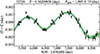 |
Fig. D.1. O − C diagram of OGLE-BLG-RRLYR-32226. Black points indicate the measured O − C values. The dashed line indicates the average solution from MCMC modeling (Hajdu et al. 2021). The shaded green regions denote the 1, 2, and 3σ credible intervals of the solutions. Above the panel, the OGLE ID, the pulsation period, and the orbital period are given. |
Appendix E: The binary parameters of OGLE-BLG-RRLYR-32226
During our analysis, we noticed that the O − C diagram of OGLE-BLG-RRLYR-32226 shows the characteristic periodic oscillation pattern expected from variables located in a binary system due to the LTTE. In fact, the binarity of this variable was already suspected during our dedicated RRL binary search (Hajdu et al. 2021), but the mean-magnitude changes were mistaken for the Blazhko effect, and it was discarded from the list of binary candidates. A more careful analysis has revealed that the light curve of the star is stable, but it is apparently affected by the LTTE and the mean-magnitude changes simultaneously, both at a relatively small amplitude. Therefore, an iterative procedure was adopted for the analysis of this star, in order to decouple these two effects in the light curve.
First, we performed an O − C analysis on the original light curve, following the Bayesian, Markov Chain Monte Carlo (MCMC) based procedure outlined in our binarity study (Hajdu et al. 2021). The timings of the light curve points were corrected with this initial O − C solution, and the resulting data were analyzed for the change in mean magnitudes as described above. Then, we repeated the O − C analysis after correcting the original light curve for the change in mean magnitudes. This solution is shown in Figure D.1, and the derived parameters are listed in Table E.1. These are: the orbital period (Porb), the projected semimajor axis (a1 sin(i)), the eccentricity (e), the argument of pericenter (ω), the pericenter passage time (T0), as well as the pulsational period change rate β. From these, we also derive the following quantities: the orbital radial velocity semi-amplitude (K1), the mass function (f(m)) and the minimum companion mass (MS, min), and also list them in Table E.1. Finally, we corrected the timings of the light curve with this second O − C solution, and reanalyzed the mean-magnitude changes, with the results of this final fit listed in Table E.1.
Binary parameters of OGLE-BLG-RRLYR-32226
All Tables
Analysis summary of the final sample of RR Lyrae stars with mean-magnitude changes.
All Figures
|
Fig. 1. Summary plot for one of the analyzed stars. Panel a: original OGLE I-band light curve folded with the period of pulsation, with the corresponding Fourier fit overlaid. Panel b: same as (a), but with the long-term changes removed. Panel c: same as (a), but for the V-band data. Panel d: same as (b), but for the V-band data. Panel e: I-band data after subtraction of the Fourier light-curve model. The orange dots and lines show the fit of the long-term changes in brightness. Panel f: same as (e), but for the V-band light curve. All light-curve points are colored according to the estimated mean-magnitude values during the observations, with lighter and darker points corresponding to brighter and fainter epochs, respectively. Above the panels, the OGLE ID, pulsation period, amplitude (ΔIDR(I)), and amplitude ratio (rI, V = A(I)/A(V)) of the mean-magnitude changes are given. The complete set of summary plots is available as online material. (see Data availability paragraph). |
| In the text | |
|
Fig. 2. Comparison of RRL mean-magnitude changes between different surveys. Each panel shows the OGLE-IV, OGLE-III, MACHO, EROS-2, MOA, and KMTNet light curves (black, blue, brown, purple, green, and red dots, respectively; see their descriptions in Appendix A) after subtraction of (separate) Fourier light-curve models for each dataset. Light curves are offset by arbitrary amounts for clarity. The overlaid orange dots and lines show the mean-magnitude change modeling according to the light-curve fits, similarly to panel (e) of Fig. 1. Above the panels, the OGLE ID, the pulsation period, the amplitude of the mean-magnitude changes, and the measured amplitude ratio rI, V = A(I)/A(V) are given for the corresponding RRL, based on the OGLE-IV data. |
| In the text | |
|
Fig. 3. Top panel: period–amplitude (Bailey) diagram of the OGLE bulge RRab sample (gray 2D histogram, shown on a logarithmic scale) and the mean-magnitude-changing RRL variables with circles colored according to the measured I-band mean-magnitude changes. Middle panel: distribution of epoch-independent phase differences (ϕ31) of the RRab stars. Bottom panel: dependency of the amplitude ratio rI, V on the amplitude of the I-band mean-magnitude changes. RRab stars are marked with circles and are colored according to their pulsation periods, while the single RRc star is marked with a black square. The horizontal dashed lines indicate the expected extinction ratios for different RV values of the standard interstellar extinction law (Cardelli et al. 1989). |
| In the text | |
|
Fig. 4. Eclipse-like event of OGLE-BLG-RRLYR-09197. Top: residual light curve of the 2008 observational season. Both pulsation and long-term mean-magnitude changes are subtracted. OGLE and MOA observations are shown with blue and green dots, respectively. For clarity, daily average magnitudes for the MOA data are also shown with orange points. Bottom: same as the top panel, but showing the event between the limits marked by vertical dashed gray lines. |
| In the text | |
|
Fig. 5. Distribution of the available I-band data points and mean magnitudes in the OGLE survey for RRab stars (black points). The stars in our final sample are marked with red circles. The dashed blue lines denote the region used to calculate the incidence rate of the mean-magnitude changing effect in RRab stars. |
| In the text | |
|
Fig. 6. Properties of the 71 RRab stars in our sample (red dots) vs. stars used for incidence rate calculation (see Figure 5). Top left: distribution of RRab stars in Galactic coordinates. Colors correspond to the V − I color of each RRab star. Top right: same as top left, but with the colors corresponding to the number of available I-band data points. Bottom left: I vs. V − I color-magnitude diagram of the RRab stars. The white arrow denotes the reddening vector for 1 magnitude of color excess for RV = 3.1 (Cardelli et al. 1989). Bottom right: proper motion distribution of the sample. The dashed white ellipse denotes the two standard deviation distances from the sample median. |
| In the text | |
|
Fig. 7. Spectral energy distributions of RRL with 8 μm photometry available. On each panel, the measured fluxes of a star are marked with red dots. The vertical and horizontal bars mark the measurement uncertainties and the effective widths of the photometric bands, respectively. The black and green curves correspond to DUSTY models with circumstellar envelopes made of amorphous carbon and silicate dust, respectively. The solid, dash-dotted, and dotted lines show progressively higher amounts of dust. Above each panel, the OGLE ID, the adopted values of V-band extinction, and distance are given. The locations of these three stars are marked by arrows on the color-magnitude diagram of the final sample (bottom-left panel of Fig. 2). |
| In the text | |
|
Fig. D.1. O − C diagram of OGLE-BLG-RRLYR-32226. Black points indicate the measured O − C values. The dashed line indicates the average solution from MCMC modeling (Hajdu et al. 2021). The shaded green regions denote the 1, 2, and 3σ credible intervals of the solutions. Above the panel, the OGLE ID, the pulsation period, and the orbital period are given. |
| In the text | |
Current usage metrics show cumulative count of Article Views (full-text article views including HTML views, PDF and ePub downloads, according to the available data) and Abstracts Views on Vision4Press platform.
Data correspond to usage on the plateform after 2015. The current usage metrics is available 48-96 hours after online publication and is updated daily on week days.
Initial download of the metrics may take a while.