| Issue |
A&A
Volume 707, March 2026
|
|
|---|---|---|
| Article Number | A220 | |
| Number of page(s) | 22 | |
| Section | Stellar atmospheres | |
| DOI | https://doi.org/10.1051/0004-6361/202558683 | |
| Published online | 17 March 2026 | |
Granulation signatures as seen by Kepler short-cadence data
I. A decoupling between granulation and oscillation timescales for dwarfs
1
Stellar Astrophysics Centre (SAC), Department of Physics and Astronomy, Aarhus University,
Ny Munkegade 120,
8000 Aarhus C,
Denmark
2
School of Physics and Astronomy, University of Birmingham,
Edgbaston B15 2TT,
UK
3
Rosseland Centre for Solar Physics, Institute of Theoretical Astrophysics, University of Oslo,
PO Box 1029, Blindern,
NO-0315
Oslo,
Norway
★ Corresponding author: This email address is being protected from spambots. You need JavaScript enabled to view it.
Received:
19
December
2025
Accepted:
9
February
2026
Abstract
Context. Granulation is the observable surface signature of convection in the envelopes of low-mass stars, forming the background in stellar power spectra. While well-studied in evolved giants, granulation on the main sequence has received less attention.
Aims. We aim to study and characterise granulation signatures of main-sequence and subgiant stars, extending previous studies of giants to provide a continuous physical picture across evolutionary stages.
Methods. We analysed 753 Kepler short-cadence stars using a Bayesian nested-sampling framework to evaluate three background descriptions and compare model preferences. This yields full posterior distributions for all parameters, enabling robust comparisons across a diverse stellar sample.
Results. No universal preference between background models is found, and thus an a priori choice is not justified. Assuming a Gaussian oscillation envelope, vmax estimates become sensitive to model misspecification, with the resulting systematics being comparable to or exceeding the formal uncertainties. The envelope width scales with vmax across models and shows a dependence on effective temperature. Total granulation amplitudes in dwarfs broadly follow giant-based scalings; however, a decoupling appears between the timescale of the primary granulation and the oscillations for main-sequence stars cooler than the Sun. The prolonged granulation timescale was reproduced by 3D hydrodynamical simulations of a K dwarf, driven by reduced convective velocities resulting from more efficient convective energy transport in denser envelopes.
Conclusions. Our study represents the most extensive Bayesian background modelling of Kepler short-cadence stars to date and reveals a decoupling between granulation and oscillation timescales in K dwarfs. The prolonged granulation timescale increases the frequency separation to the oscillation excess, potentially aiding seismic detectability, while the reduced convective velocities may influence the excitation of stellar oscillations and relate to the low amplitudes observed in cool dwarfs. Finally, we contribute a dataset linking granulation, oscillations, and stellar parameters, establishing a foundation for future investigations into their interdependence across the Hertzsprung–Russell diagram.
Key words: asteroseismology / stars: atmospheres / stars: evolution / stars: interiors
© The Authors 2026
 Open Access article, published by EDP Sciences, under the terms of the Creative Commons Attribution License (https://creativecommons.org/licenses/by/4.0), which permits unrestricted use, distribution, and reproduction in any medium, provided the original work is properly cited.
This article is published in open access under the Subscribe to Open model. This email address is being protected from spambots. You need JavaScript enabled to view it. to support open access publication.
1 Introduction
Stellar granulation is the photometric signature of convection in the outer layers of stars with convective envelopes. Hot plasma rises towards the photosphere, cools, and sinks back into the stellar interior, producing a dynamic pattern of bright granules and darker intergranular lanes. These motions occur on characteristic timescales set by the fundamental stellar properties, reflecting the interplay between gravity, temperature, and composition in the outer layers, resulting in the introduction of a stochastic signal in photometric time series. In the frequency domain, granulation manifests as a background in the power density spectrum (PDS) that decays with increasing frequency and is often modelled by Harvey-like functions (Harvey 1985). The high precision and long baselines of space-based missions such as Kepler (Borucki et al. 2010) have made it possible to measure granulation parameters for large numbers of stars with a wide range of fundamental properties.
Granulation has been extensively characterised in the Sun (e.g. Karoff et al. 2013), where high signal-to-noise (S/N) data allow detailed modelling of the temporal and spatial properties of convection. In evolved stars, Kallinger et al. (2014) analysed thousands of Kepler red giants, establishing empirical scaling relations between granulation parameters and the global asteroseismic quantity known as the frequency of maximum oscillation power, νmax. Working purely in the time domain, Rodríguez Díaz et al. (2022) evaluated the autocorrelation time of the Legacy stars (Lund et al. 2017), pushing towards studying the granulation of main-sequence (MS) stars. In doing so, they found that the scaling laws roughly agree with those of Kallinger et al. (2014). Parallel theoretical and numerical work, notably 3D radiative hydrodynamical simulations of stellar atmospheres, has provided physical justification for those scaling relations and allowed for the exploration of their dependence on metallicity, surface gravity, and convection prescription (Samadi et al. 2013; Zhou et al. 2021). Yet, the stellar samples where detailed granulation studies have been performed primarily consist of more evolved stars on the late-subgiant (SGB) and red-giant branch (RGB).
Extending granulation studies to MS and less-evolved SGB stars is essential for establishing how surface convection scales across different stellar regimes. Whereas current empirical scaling relations are largely informed by evolved stars, the behaviour of granulation in less-evolved stars is not as well characterised. MS and SGB stars probe a broad range of temperatures, surface gravities, and Mach numbers, providing an ideal setting to examine whether the empirical relations derived from red giants remain valid when applied to hotter, denser stellar envelopes. By analysing the granulation signatures in frequency space for the largest sample of MS and SGB stars to date, this work bridges the observational gap between dwarfs and giants and offers new constraints on how granulation properties evolve with stellar structure. This calibration has immediate significance not only for convection theory, but also for asteroseismic applications – such as improved background modelling for upcoming missions (e.g. the PLAnetary Transits and Oscillations of stars, PLATO; Rauer et al. 2025) and a refined understanding of seismic detectability in cool MS stars – and more reliable noise characterisation in precision exoplanetary studies.
Larsen et al. (2025) introduce a Bayesian nested-sampling framework for evaluating competing granulation background models using 3D radiative hydrodynamical simulations, and demonstrate its potential through limited application to stellar observations. Their analysis shows that the accuracy and robustness of comparisons between granulation background models might be obscured by the commonly adopted Gaussian envelope model for the oscillation excess that sits atop the background profile. Further development was therefore required before reliable application of the framework to large, heterogeneous observational datasets. In this work, we extended the application of the framework to a catalogue of Kepler short-cadence stars by Sayeed et al. (2025), spanning a wide range of evolutionary states, observing durations, and signal-to-noise ratios (S/Ns).
This work first presents the stellar sample studied in Sect. 2. The further developments to the framework of Larsen et al. (2025) are outlined in Sect. 3, which also details the methodology underlying this study. In Sect. 4, we investigate the model preferences and sensitivities across the sample, before studying in detail the scaling of the granulation parameters for MS and SGB stars in Sect. 5. In doing so, we uncover what appears to be a previously unreported decoupling between granulation and oscillation timescales – a result that motivates a dedicated extension of the sample in Sect. 6 with additional K dwarfs observed by the Transiting Exoplanet Survey Satellite (TESS; Ricker et al. 2014) and theoretical considerations using both 1D and 3D K-dwarf models. Finally, in Sect. 7 we make our concluding remarks and outline potential future implications of our findings.
2 Kepler short-cadence sample
The sample used in this work was drawn from the catalogue of Sayeed et al. (2025). The catalogue consists of all known solar-like oscillators observed in short-cadence mode by Kepler and numbers a total of 765 stars – primarily sourced from the Legacy (Lund et al. 2017), KAGES (Silva Aguirre et al. 2015), and APOKASC (Serenelli et al. 2017) catalogues. Figure 1 shows the distribution of these stars in a Kiel diagram. The sample is dominated by MS and SGB stars, but also includes a modest number of stars on the lower RGB. Importantly, there are several G and K dwarfs present situated in the vicinity of and lower on the MS than the Sun, respectively.
This catalogue provides ample grounds for further development and testing of the framework presented in Larsen et al. (2025) – see Sect. 3 for details – as it contains a large number of stars spanning a broad range of evolutionary stages across the MS, SGB, and the lower RGB; whereas previous similar studies focused largely on evolved stars observed by Kepler in long cadence (Kallinger et al. 2014). Furthermore, for most stars in the catalogue a seismic characterisation exists. This means that the global asteroseismic parameters −vmax and the large frequency separation Δ v – are largely available, as well as seismically determined masses, radii and ages for the majority of the sample. In short, the catalogue studied in this work consists of some of the most well-characterised dwarf stars observed by Kepler.
For the entire catalogue of Sayeed et al. (2025), we retrieved the raw Kepler data for all targets and processed them with the KASOC filter (Handberg & Lund 2014) to ensure a homogeneous treatment of the data. The corresponding power density spectra were then computed following the approach of Handberg & Campante (2011). Known Kepler systematics were removed based on the list provided in Table 5 of the Kepler Data Characteristics Handbook (Van Cleve et al. 2016). To mitigate the influence of strong rotational variability, we omitted PDS data below 10 μHz, corresponding to rotational signatures with periods longer than approximately 1.15 days. For our sample of Kepler short-cadence stars – composed primarily of low-mass MS and SGB stars (see Fig. 1) – rotation periods shorter than about 1.15 days are unlikely (Santos et al. 2024). While some harmonics of the rotational peaks may extend into the low-frequency regime, their contribution to the overall power budget is minor, and the activity component of our background models effectively absorbs their influence on the granulation signal.
The sample spans stars with Kepler observations ranging from less than a single quarter (≲ 30 days) to over three years. Some of the more evolved stars with short time series may have longer-duration long-cadence data available, which could improve PDS quality. Nevertheless, we restricted this analysis to the short-cadence data to maintain consistency. Applying the Larsen et al. (2025) framework to a broad range of stars including lower-quality cases – and as we were focusing on granulation rather than pulsation features – provided a stringent test of the method and supported the further developments outlined in Sect. 3.
Before moving on, we note that the catalogue of Sayeed et al. (2025) contained a few stars not suitable for our work. The specific stars which were removed from the sample and the associated reason(s) can be found in Table A.1. As will become clear in Sect. 3, we use an estimate of the observed νmax for our setup and prior definitions. We took the following steps to obtain them, listed in order of priority:
vmax directly from Table 3 of Sayeed et al. (2025) taken from literature estimates.
vmax from source papers if applicable (Silva Aguirre et al. 2015; Lund et al. 2017; Serenelli et al. 2017).
vmax estimated by pySYD (Chontos et al. 2021) from Table 3 of Sayeed et al. (2025).
Recover Δ v and Teff estimates from Tables 3 and 4 of Sayeed et al. (2025), respectively, and calculate vmax using the asteroseismic scaling relation (Eq. (D.1)).
Through the steps above, we recovered a νmax estimate for all stars in the sample. However, as we were dealing with short-cadence Kepler data and considered stars on the MS, SGB and lower RGB, we chose to discard the star if the estimated vmax<100 μHz, indicating an evolved giant star. In summary, the discarded stars in Table A.1 number 12 in total and contain both those deemed unsuitable and those below the adopted vmax cut-off. This resulted in a reduced sample of 753 stars for our studies.
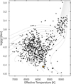 |
Fig. 1 Kiel diagram of the 733 stars with available effective temperatures and surface gravities, taken from the sample after the sorting in Sect. 2. The Teff values are retrieved from Table 3 of Sayeed et al. (2025), while the seismic log g was calculated using the asteroseismic scaling relations with this Teff and the Δ v estimate from Sayeed et al. (2025). Simple stellar evolution tracks of solar metallicity and a range of masses are overplotted to guide the eye. The solar location is indicated by the yellow star symbol. |
Background models used in this work, presented in an adapted version of Table 1 from Larsen et al. (2025).
3 Framework and methodology
The foundation of the framework for performing the background model inference was developed and described in Larsen et al. (2025). It is a Bayesian setup based on nested sampling using the inference algorithm Dynesty (Speagle 2020), which allows simultaneous estimation of the posterior probability distributions and the Bayesian evidence, 𝒵. For details on the main body of the framework we refer to Larsen et al. (2025). Specifically, their Sect. 2.2 outlines the complete description of stellar power spectra including how apodisation (Chaplin et al. 2011), stellar activity, oscillations, and white noise is accounted for (see also Appendix C). Herein, we describe the further developments enabling extensive application to the Kepler shor-tcadence sample. The developments are described in Sect. 3.1 and Appendix E, and also concern refined priors (see Appendices B and C). The background models considered in this work are those concluded in Larsen et al. (2025) to have merit and are seen in Table 1: a hybrid model with a single amplitude and two characteristic frequencies (J), a two-component Harvey model (H) and a three-component Harvey model (T).
In Larsen et al. (2025), the framework was applied primarily to 3D hydrodynamical simulations of convection, but subsequently extended to two real stars: the solar analogue KIC8006161 (Doris) and the Sun. These stars were of exceptionally high quality and S/Ns. Applying the framework widely to our sample of 753 stars requires handling cases where the PDS components are less distinct, necessitating further developments of the framework. The setup we developed encodes physically motivated connections between the various components of power density spectra and is outlined in Sect. 3.1. Moreover, Larsen et al. (2025) noted that the conclusions drawn on the background model preference may depend on the implemented model for the power excess due to the presence of stellar oscillations. To investigate this, we present extensive tests of a new approach dubbed ‘peakbogging’ to account for the oscillation excess, briefly summarised in Sect. 3.3 and outlined in detail throughout Appendix E. Both the traditional treatment using a Gaussian envelope and peakbogging utilise the developments in Sect. 3.1.
The log-likelihood ln ℒ used throughout this work describes independent frequency bins in the PDS combined with a standard χ2 probability distribution. In the present work, the likelihood defined in Larsen et al. (2025) is slightly modified to allow for binning of the PDS by introducing the factor s as the number of datapoints per i ’th bin into the expression for χ2 (see e.g. Appourchaux 2004; Handberg & Campante 2011; Lundkvist et al. 2021), such that
 (1)
(1)
 (2)
As in the original framework of Larsen et al. (2025), D denotes the observed data (power), θ is the model parameters and M an assumed model predicting a power Mi(θ) for a given frequency bin.
(2)
As in the original framework of Larsen et al. (2025), D denotes the observed data (power), θ is the model parameters and M an assumed model predicting a power Mi(θ) for a given frequency bin.
3.1 A correlated inference setup
It is well known that vmax is closely linked to both the amplitudes and characteristic timescales of granulation, as all three quantities reflect the properties of the underlying convective motions (e.g. Kjeldsen & Bedding 2011; Mathur et al. 2011; Samadi et al. 2013; Kallinger et al. 2014; Rodríguez Díaz et al. 2022). This physical connection implies that these parameters are correlated and unlikely to vary independently during our inference: a star with a low vmax must also exhibit granulation with correspondingly larger amplitudes and longer timescales, while a high vmax demands the opposite.
In our framework, this correlation provided a natural way to let the PDS as a whole guide the sampling. When we consider the entire PDS – spanning several orders of magnitude in both frequency and power – the inference is naturally sensitive to any combination of vmax and granulation parameters that fails to reproduce the overall behaviour of the spectrum. For instance, a MS-like vmax paired with granulation amplitudes of several hundred parts-per-million and timescales of only tens of microhertz would contradict the expected behaviour. During the sampling, any tentative move towards such mismatched parameter combinations should therefore result in a disfavoured likelihood given the data, effectively steering the sampler away from unphysical regions of parameter space.
To implement this, we developed a correlated inference setup for the granulation parameters for which scaling relations with vmax were derived by Kallinger et al. (2014) – which is the amplitude, a, and timescale, b, of the first granulation component and the timescale, d, of the second. This means that instead of freely sampling the granulation parameters, we calculated them based on the sampled vmax. In turn, we controlled the strength of this correlation by adding a scatter parameter to be inferred:
![Mathematical equation: $a[\mathrm{ppm}]=3382 v_{\text {max }}^{-0.609} \sigma_{a},$](/articles/aa/full_html/2026/03/aa58683-25/aa58683-25-eq6.png) (3)
(3)
![Mathematical equation: $b[\mu \mathrm{~Hz}]=0.317 v_{\text {max }}^{0.970} \sigma_{b},$](/articles/aa/full_html/2026/03/aa58683-25/aa58683-25-eq7.png) (4)
(4)
![Mathematical equation: $d[\mu \mathrm{Hz}]=0.948 v_{\max }^{0.992} \sigma_d.$](/articles/aa/full_html/2026/03/aa58683-25/aa58683-25-eq8.png) (5)
The power-law coefficients come from Kallinger et al. (2014) and vmax is a free parameter during the inference. The scatter parameters, σa, b, d, describe the potential scatter of the scaling relations and are also freely sampled. Priors forcing the scatter parameters close to 1 imposes a very tight correlation, while allowing wider variation from 1 lessens the correlation between granulation and vmax. Inspecting Fig. 8 of Kallinger et al. (2014), we see that the scatter for their RGB sample is quite low and roughly symmetric in the log-parameters; ∼10−15% for the timescales and ∼15−30% for the amplitude. These considerations are carefully taken into account when defining the prior ranges for σa, b, d in Appendix C.
(5)
The power-law coefficients come from Kallinger et al. (2014) and vmax is a free parameter during the inference. The scatter parameters, σa, b, d, describe the potential scatter of the scaling relations and are also freely sampled. Priors forcing the scatter parameters close to 1 imposes a very tight correlation, while allowing wider variation from 1 lessens the correlation between granulation and vmax. Inspecting Fig. 8 of Kallinger et al. (2014), we see that the scatter for their RGB sample is quite low and roughly symmetric in the log-parameters; ∼10−15% for the timescales and ∼15−30% for the amplitude. These considerations are carefully taken into account when defining the prior ranges for σa, b, d in Appendix C.
3.2 Studying granulation for a large sample
Our sample of 753 stars exhibits substantial diversity. Our focus is on characterising the stellar granulation background – the broad trends in the power density spectra across several orders of magnitude in frequency and power – rather than resolving the detailed structure of the oscillation modes. This emphasis naturally motivates moderate binning of the power density spectra, providing consistent resolution across the sample and smoothing statistical fluctuations.
Binning offers several advantages. Averaging multiple independent frequency bins causes the noise distribution to converge toward a Gaussian by the central limit theorem (Laplace 1812), replacing the exponential distribution characteristic of individual PDS bins (Anderson et al. 1990). This transformation improves sampling stability and effectiveness, since the sampler no longer needs to account for a highly skewed distribution. The corresponding χ2 statistics of Eq. (2) are adjusted via the effective degrees of freedom, s=2 N, with N being the number of independent points per bin. We tested the impact of varying the binning by examining how the inferred granulation parameters respond to changes in bin size. We focused on the second granulation component, which is most sensitive to changes in resolution, as it describes the frequency range near the stellar oscillations. We applied model H (Table 1) to three stars: KIC 6679371, KIC 8866102, and KIC 8006161 with values of vmax ∼1000, 2000, 3500 μHz, respectively. The binning was varied to provide frequency resolutions ranging from 0.025 to 4.5 μHz. Variations in the inferred parameters remained below the associated 1 σ uncertainties, demonstrating that the choice of binning does not meaningfully bias the measurements.
The main trade-off when binning is that low-amplitude oscillation peaks, especially in the envelope wings, may be partially smoothed. However, these features contribute negligibly to the total power budget and thus have little impact on our granulation inferences. Furthermore, as an added bonus, binning improves computational efficiency by reducing the number of data points, substantially decreasing runtime for each inference. Several stars in our sample have time series shorter than a full Kepler quarter, yielding a native frequency resolution ∼0.4 μHz. For stars with sufficiently long time series, we bin the PDS to a uniform resolution as close as possible to 0.5 μHz, while maintaining a constant number of data points per bin, N, to ensure consistent and robust χ2 statistics. This choice is made throughout this work and balances the need for statistical stability and computational tractability, while retaining the granulation signals of interest.
Figure 2 shows the outcome of applying model H and binning to a resolution of 0.5 μHz for KIC 6679371, KIC 8866102, and KIC 8006161. This figure visualises the results we will obtain – here for model H, however repeated for J and T as well for every sample star considered in this work using the outlined framework. We see how the two Harvey profiles describe the lower and upper granulation components at increasing frequencies, with the Gaussian envelope standing on top of the inferred background slope. By inspection of KIC 8006161 in the bottom panel, we notice that the primary granulation component at lower frequency is both prominent and very clearly separated in frequency from the oscillation excess. Through the study of similar stars this trend will be assessed more thoroughly in Sect. 6, but already here one may notice that this wide a separation in frequency is not readily apparent for the other two more evolved stars in Fig. 2. The choice to remove the PDS contributions below 10 μHz in order to avoid the influence of strong rotational peaks only plays a role for KIC 8866102 in the middle panel. However, true for all three is that this choice does not affect the remaining granulation and oscillatory parameters, as the lowest frequency regime remains adequately described by the activity component. Finally, we see that the effect of binning the PDS does indeed increase the contrast without affecting the finer details of the inference.
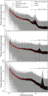 |
Fig. 2 Power density spectra with overlaid results of the background model inference using model H (see Table 1) when binning to 0.5 μHz resolution for three stars: KIC6679371 (top), KIC8866102 (middle), and KIC8006161 (bottom). The unbinned PDS is shown in grey with the binned version overplotted in black. The model is plotted in red using the median of the obtained posteriors for each fit parameter. Additionally, 50 randomly drawn samples from the posteriors are used to replot the model to indicate the scatter. The individual granulation components are plotted as dashed green profiles. The fitted value of vmax is given in each panel and indicated by the vertical dashed black line, while the noise is shown by the horizontal dashed orange line. The activity component is the dash-dotted green line. The model without the influence of the Gaussian oscillation excess is plotted as the dashed blue profile, visible underneath the oscillation excess. |
3.3 Introducing peakbogging
Traditionally, the oscillation excess is represented with a symmetric Gaussian envelope atop the granulation background, yet such an approach may be problematic. This can systematically misrepresent the power distribution, particularly when (i) the envelope is intrinsically asymmetric, (ii) mode visibilities are non-standard (e.g. due to inclination, mode lifetime or mixedmode complexity), or (iii) the available data has a low S/N and sparse sampling. In such cases the Gaussian envelope may trade off with the background model and misrepresent the true power distribution, thereby biasing granulation amplitudes and timescales, which might in some cases lead to degeneracies between the background and oscillation components. The issues associated with the traditional Gaussian approach also affected the results of Larsen et al. (2025), where it was discussed if the conclusions on model preference may depend on how the oscillation excess is accounted for.
These limitations motivated the development and testing of the so-named peakbogging approach: a mixture-model likelihood setup where a flexible foreground component absorbs residual signal not described by the assumed background model, aimed at reducing the bias associated with background model choices and improving robustness when applied across diverse stellar samples. However, as is discussed in Appendix E.7, certain unresolved pathologies plague peakbogging when applied to the sample studied in this work. On the other hand, it shows promise for a significant number of stars and is robust in terms of providing meaningful posteriors. Moreover, in virtually all cases peakbogging recovers an identical estimate of the total granulation amplitude (Sects. 5.1 and E.6).
The detailed setup of peakbogging is outlined in Appendix E, and throughout the appendix we present the peakbogging results analogous to those in the main paper, while discussing the promising aspects alongside the potential issues. For the results presented in the remainder of this article, we utilised the traditional approach of treating the oscillation excess using a Gaussian envelope. We acknowledge the underlying assumptions and misrepresentations of this model in doing so.
4 Background model preferences and sensitivities across the sample
By applying the granulation background inference framework to the sample outlined in Sect. 2, we can now begin to investigate the trends exhibited by the granulation and oscillatory components across a diverse set of MS, SGB, and lower RGB stars. Inevitably, when analysing such a large and diverse sample in detail, a small fraction of stars cannot be recovered with reliable results, typically due to a combination of short time series and low S/N, contamination from spurious peaks in the PDS, or numerical convergence issues in the nested sampling procedure. To ensure that only robust results enter our analysis, we evaluate the quality of the posterior distributions obtained for all granulation parameters and retain only those that are well-sampled and statistically consistent. This conservative approach ensures that the inferred model parameters – estimated as the median of the posterior distributions, with corresponding uncertainties from the 16th and 84th percentiles – represent genuine features of the data rather than artefacts of a failed inference. In our case we discard the star if any of the three background model inferences fail, as proper subsequent comparisons are unable to be made. We note in passing that sometimes a star is thus discarded where a subset of the three considered background models did provide valid results. In total 4 targets failed to yield meaningful inferences and were removed. Hence, in the remainder of the paper we present results based on the remaining 749 stars. These stars thus provide a data sample where the complete posterior distributions for all parameters, the covariances between the parameters, and the Bayesian evidence 𝒵 are readily available for study herein and in future efforts.
In the following we first examine the background model preferences of the individual stars, as quantified by the Bayesian evidence obtained through nested sampling. We then assess how the choice of background model affects the inferred vmax values, before inspecting how the width of the oscillation excess changes across the evolutionary stages of the sample. Specifically for the latter two investigations in Sects. 4.2 and 4.3, we evaluated the resulting vmax estimates and Gaussian envelope widths to further sort the dataset. In cases where the oscillatory signal is unclear the Gaussian envelope model is a poor representation of the data and may perform badly. When it does, the framework attributes negligible power to the Gaussian envelope and essentially removes its contribution by narrowing it in to absorb a single noise peak. In such cases the oscillations contribute negligibly to the overall power budget, meaning that the underlying granulation background components are still well-characterised. Yet for investigations of νmax and the oscillation excess widths, such cases were removed from consideration.
4.1 Background model preferences
Previous efforts have considered how the choice of background model has implications for the resulting outcome and our conclusions in connection to observational asteroseismology (see e.g. Sreenivas et al. 2024). Specifically, Handberg et al. (2017) discussed such aspects and argue how a single choice of background model may not be suitable. They argue that fixing the background model a priori carries the assumption that the model accurately describes the granulation background for the star(s) in question – an assumption that is hard to justify for such a diverse sample as the one studied in this work.
By applying the three different background models of Table 1 to the entire sample, we thereby avoid this assumption. Figure 3 shows that the assumption of a single background model being suitable is not justified, even in restricted regions of stellar evolution. Across the sample, models H and T – the two- and three-component Harvey models, respectively – are consistently preferred over the hybrid model J. No readily apparent trends in model preference across the different evolutionary stages are seen in the figure. Hence, if the goal is to most accurately describe the granulation background for a certain dataset – be it to study the granulation itself or correct for the background to study the oscillations – these results indicate that one must consider various models and choose the one which best represents the data.
In Larsen et al. (2025), it was briefly discussed whether the conclusions regarding model preference depend on the assumption of a Gaussian envelope representing the oscillation excess. Similarly, in the present analysis, we cannot exclude the possibility that the inferred preferences depend on this assumption. We also note that Fig. 3 displays evidence ratios, not posterior odds ratios, which would additionally include a factor reflecting our prior beliefs. In other words, the results shown purely indicate which model best fits the data, without accounting for physical plausibility or other prior reservations concerning the assumed background models. For instance, some readers may question the three-component model T, whose third granulation component appears at high frequency (v ≳ vmax). If so, such prior beliefs should be incorporated when interpreting Fig. 3, potentially shifting the preference towards models J or H.
As a further consequence of relying on a Gaussian envelope, we occasionally find that the granulation components compensate for its shortcomings when describing the power around the oscillation excess. In such cases, the model effectively trades power between the granulation terms and the envelope because the latter provides only a crude approximation to the true oscillation signal. This behaviour naturally raises the question of whether the inferred model preferences are influenced by the chosen representation of the oscillation excess. To explore this, Appendix E.5 presents an analogous analysis based on the peakbogging approach (Fig. E.2), which offers a more flexible description of the oscillation power. Although peakbogging has its own unresolved issues, Fig. E.2 demonstrates that the preferred background model can change when the oscillation excess is represented differently. Consequently, as the preferred model is sensitive to the underlying assumptions, this reinforces the need to avoid a priori selection of a background model and instead choose the optimal model on a star-by-star basis (Handberg et al. 2017).
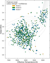 |
Fig. 3 Kiel diagram with colouring according to normalised evidence ratios, with model preferences as indicated by the legend. When models are comparable in their evidences the colour is blended between the two competing models. The Sun is overplotted as the enlarged star symbol at the solar location and significantly prefers model T. |
4.2 Background model sensitivity of vmax
In asteroseismic studies of the stellar background signal, a key parameter used for subsequent analysis is vmax. Thus, the question of how vmax varies with the assumed background model naturally arises. In Fig. 4 we present the fractional differences in vmax between the different models. To keep the results internally consistent, we compare to the value obtained with our framework when using the most widely applied model in literature, that is, the two-component model H, rather than the observed values from Sayeed et al. (2025).
It is readily apparent that variations between the models occur. Specifically, a slight tendency is seen for lower vmax estimates when using the hybrid model J in comparison to model H. The root-mean-square scatter is also slightly larger when the nature of the model changes from individual Harvey-like components to the hybrid model. For the majority of the sample, the variations are below the ∼2% level. However, some stars show larger variation up to and exceeding the ∼5% level when changing the assumed background model. For the comparison between models T and H, the residuals are consistent with zero within 2 σ formal uncertainties for 93% of stars, but for J vs H this decreases to 79% (meaning 21% show inconsistencies that cannot be explained by formal uncertainties alone). Hence, while the formal uncertainties – with mean fractional values of ∼1.5% – explain the scatter for the majority of the sample, there is a significant number of cases where they do not.
When using a framework such as in this work, or alternatively pipelines such as pySYD (Chontos et al. 2021), the internal uncertainties reported on vmax are often very small. The above recovery percentages indicate that the choice of background model introduces systematic differences that are comparable to or dominating the formal uncertainties reported on vmax.
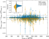 |
Fig. 4 Comparison of the vmax determination across the different models. The vmax fractional residuals of models J and T to those obtained by model H are plotted in yellow and blue, respectively. The horizontal dashed line indicates perfect agreement in vmax determinations, while the dot-dashed show the 2% bounds. The RMS scatter was calculated for both cases and is provided in the inserted box in the top right. The insert shows a split violin plot of the vmax residual distributions for model J (left) and model T (right) versus model H, with medians and 16th/84th percentiles overplotted as full and dashed horizontal lines, respectively. |
4.3 Oscillation excess widths
Having applied the Gaussian envelope approach to the entire sample we have obtained estimates of the oscillation excess widths σ for, to our knowledge, the largest collection of Kepler MS and SGB stars to date. How the width of the oscillation excess changes through evolution has been studied by e.g. Stello et al. (2009b) and Mosser et al. (2012). This sample, however, enables a future study of how the oscillations widths depend on various stellar parameters such as temperature, metallicity, or stellar masses.
Figure 5 shows the obtained full-width-half-maxima, FWHM  , of the Gaussian envelopes obtained by the background model inferences. It can be seen how across all models, the trend suggested by Stello et al. (2009b) as vmax/2 seems to provide a rough upper boundary. Furthermore, the trend FWHM
  suggested by Mosser et al. (2012) follows much of the data, but significant scatter around the relation is found. For model J specifically, larger oscillation widths are found for the stars with νmax ≳ 2000 μHz.
Lastly, we note a trend with temperature, indicating that lower effective temperatures correspond to smaller oscillation excess widths (as also noted by (Schofield 2019)). Exploring empirical scaling relations for oscillation widths that account for temperature or other stellar parameters, and potentially include subdivisions by evolutionary stage as considered by Kim & Chang (2021), would be an interesting avenue for future work using the provided dataset.
5 Scaling of granulation parameters
In this section we will study how the granulation behaves across the sample, similarly to how Kallinger et al. (2014) approached it for their sample of Kepler RGB stars. For brevity we restrict ourselves and only consider the total granulation amplitudes predicted by the background models, which means the combined amplitudes of the individual granulation components. Furthermore, we then study the characteristic frequencies (i.e. timescales) associated with each granulation component across the different background models of Table 1.
5.1 Total granulation amplitudes, Agran
The total granulation amplitude includes the bolometric correction for the Kepler passband, defined as  , where each ai denotes the normalised granulation amplitude of an individual component after accounting for apodisation, and Cbol=(Teff/5934 K)0.8 (Michel et al. 2009; Ballot et al. 2011). The top row of Fig. 6 shows these amplitudes for the 727 stars in our sample with available Teff measurements. The total power attributed to granulation varies only marginally among the different background models, and this stability of Agran demonstrates the internal consistency of our framework.
Following the approach of Kallinger et al. (2014), we fitted a simple power law to the measured Agran values as a function of vmax. The resulting scaling relations derived for Agran for each background model (the fit coefficients are indicated in the figure) show the same picture: a declining amplitude with increasing vmax and an exponent similar to −1/2. Moreover, despite widely applying this simplistic and naive power law description to the entire sample, the resulting scaling relations qualitatively agree with those obtained by Kallinger et al. (2014), however with a less steep slope. As Kallinger et al. (2014) focused on evolved RGB stars, while our sample is dominated by less-evolved SGB and MS stars (see Fig. 1), this may indicate an evolutionary effect on the slope. However, further work would be required to confirm this statement, as the background model used by Kallinger et al. (2014) (their model F) is not identical to, and is more constrained than, any of the models considered here.
Several theoretical studies have examined how metallicity, [Fe/H], affects granulation amplitudes, typically predicting lower amplitudes for more metal-poor stars (Corsaro et al. 2017; Yu et al. 2018; Rodríguez Díaz et al. 2022). In Fig. 6, the amplitudes are colour-coded by metallicity where available. Despite recognising that the range in [Fe/H] is modest, no systematic trend with metallicity is apparent. However, as also noted by Kallinger et al. (2014), the amplitudes are expected to depend on stellar mass: at a fixed vmax, higher-mass stars should exhibit smaller amplitudes than lower-mass ones. This mass dependence likely contributes to the scatter seen in Fig. 6, and may obscure any subtle metallicity trend that could otherwise emerge.
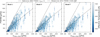 |
Fig. 5 FWHM of the Gaussian oscillation excess as a function of the determined vmax, coloured by the temperature of the star. The dashed and dot-dashed lines indicate the predictions by Stello et al. (2009b) and Mosser et al. (2012), respectively. |
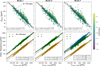 |
Fig. 6 Total granulation amplitudes and characteristic frequencies as a function of vmax obtained for the three background models of Table 1. In all panels, the dashed lines represent the corresponding scaling relation for the parameter from Kallinger et al. (2014). Top row: total granulation amplitudes colour-coded by the stellar metallicity [Fe/H] for the 727 stars with available temperatures. The black lines show a power law fit to the data. Bottom row: the characteristic frequencies of the individual granulation components for the 749 stars with consistent granulation posteriors, with colours as indicated by the legend. The corresponding coloured lines show the results of a power law fit to the data for each timescale, all given a black outline for improved readability. |
5.2 The granulation timescales for dwarfs
A close correlation between the granulation timescale (or equivalently, the characteristic frequency, v=1 /(2 π τ)) and vmax is expected from theoretical considerations; a trend that was utilised earlier in Sect. 3.1. This relationship is shown in the bottom row of Fig. 6 for the three background models. In all cases, the characteristic frequencies increase with vmax. Interestingly, the third component of model T also follows this trend, with a scatter comparable to that of the secondary component, which lends some credibility to its presence at high frequency.
For the primary granulation component, however, the MS and SGB stars lie systematically above the scaling relation of Kallinger et al. (2014). Following the same procedure as for Agran, we fitted a simple power law to the characteristic frequencies of the first (b), second (d), and third (f) granulation components for each background model. The resulting fit coefficients are given in the figure panels. For the primary granulation component, clear systematic deviations from these fits indicate that, for our Kepler short-cadence sample, a simple power-law scaling does not adequately capture the observed behaviour. The most evolved stars in the sample at low values of vmax lie systematically below, meanwhile the MS and SGB stars hint at a non-linear trend in this log-space figure.
The most striking deviation occurs for the primary granulation component at high vmax, from roughly the solar value (νmax ≈ 3000 μHz) upwards, corresponding to MS stars cooler than the Sun. Across all background models, the characteristic frequency – or equivalently, the granulation timescale – appears to reach a plateau. This flattening implies that the tight correlation between granulation timescale and νmax breaks down, which would manifest in the stellar power spectra as an increasing frequency separation between the primary granulation component and the oscillation excess. Such behaviour was already noted for KIC8006161 in Fig. 2, which indeed lies on this plateau. The departure from this otherwise robust correlation is intriguing, as both granulation and stellar oscillations are fundamentally governed by the convective motions of the star. We further investigate this phenomenon and its implications in more detail in Sect. 6.
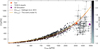 |
Fig. 7 Timescale of the primary granulation component against the oscillation timescale vmax, indicating a decoupling through a plateau beyond vmax ≈ 3000 μHz. The plotted values are those estimated by the background model preferred by the Bayesian evidence 𝒵. The Kepler sample is replotted from Fig. 6. The TESS K-dwarf additions are shown as the triangular points with black outlines. The Sun is shown as the dark orange star symbol, obtained using a ∼3.15 year time series from VIRGO (Fröhlich et al. 1995) blue band data taken during the solar minimum between solar cycle 23 and 24. Lastly, a STAGGER (Stein et al. 2024) 3D hydrodynamical simulation replicating the K-dwarf ε Indi A is shown as the purple diamond. The colouring indicates an S/N-proxy as the ratio between the estimated granulation amplitude level and the white noise, where stars exhibiting higher degrees of contrast are darker. |
6 Investigating the granulation plateau with TESS and stellar modelling
In Sect. 5.2 we found an indication of a plateau in the granulation timescale for stars with a vmax ≳ 3000 μHz. We wish to investigate this surprising trend further, as it indicates a potential decoupling between granulation and oscillation timescales for cool dwarfs. The apparent plateau in Fig. 6 relies on a modest number of stars, as only a few in the sample display vmax ≳ 3000 μHz. To remedy this situation, we further populate it with K-dwarfs observed by TESS (Ricker et al. 2014). The target selection and data retrieval is outlined in Appendix D.
Compared to Kepler, TESS delivers shorter time series with lower photometric contrast, which inevitably reduces the overall quality of the corresponding power spectra. For our purposes, however, the primary signal of interest is the granulation rather than the oscillations. While the latter are typically too weak to be detected reliably in TESS data of K-dwarfs (except for a few cases: Hon et al. 2024; Lund et al. 2025), the granulation may remain accessible. To ensure that these signals are not constrained by assumptions tailored to spectra that display clear oscillation signatures, we disable the correlated-inference configuration of Sect. 3.1, allowing the granulation parameters to be freely inferred.
After application of the framework we manually evaluated all 78 stars. Those dominated by white or blue noise, displaying strong contaminants at low frequency, or miniscule granulation signals were removed. All posteriors for the stars were subsequently inspected to ensure reliable sampling and meaningful posteriors. In total, this removed 16 stars such that the TESS K-dwarf additions numbered 62, which are seen in Fig. 7. The results obtained for the TESS K-dwarfs are plotted using the scaling relation vmax estimates and uncertainties, not the vmax inferred by the framework, as the oscillatory signals were undetectable.
The TESS K-dwarfs reproduce the plateau and thus lend further credibility to the decoupling between the granulation and oscillation timescales. As expected they show a larger scatter and a generally more uncertain estimation of the plateau, owing to the worse quality of the photometry. The stars showing the largest uncertainties in the estimated timescale similarly display granulation amplitudes comparable to the white noise level. Lastly, we examined the Gaia activity indexes (Creevey et al. 2023) for the stars in Fig. 7 to evaluate if magnetic activity could play a role in the observed scatter. However, no clear trend with the activity levels was found. While the scatter for the TESS K-dwarf additions is large, it is notable that the majority lie well below the expected scaling relation with vmax. Furthermore, they scatter to quite low values, indicating significantly longer timescales than expected.
6.1 Signal recovery using simulated power spectra
To validate that the framework can robustly recover granulation signals in power spectra with low S/Ns, we performed a recovery test. We selected all Kepler and TESS targets shown in Fig. 7 with vmax>3000 μHz − 73 stars in total – and simulated their power spectra using whichever background model was preferred by the evidence.
For each star, we adopted the observational parameters inferred by the framework as the underlying ‘true’ signal and added χ2-distributed noise following Gizon & Solanki (2003). We then generated six noise realisations per star with white-noise levels corresponding to target S/Ns = observed primary granulation amplitude/white noise = {5.0, 2.0, 1.0, 0.7, 0.4, 0.2, 0.1}. In total, this yielded 511 simulated spectra: 259 generated using model J, 153 using model H, and 98 using model T. That the simplest model (J) is preferred for the TESS data, which overall displays lower contrast between granulation and white noise levels than the Kepler data, is in line with the findings by Kallinger et al. (2014).
We then reapplied the framework to all simulated spectra using the same background model that generated them and evaluated how well the characteristic frequency of the primary granulation component, b, was recovered. While all background parameters could be tested, b is most relevant here, as the observed decoupling hinges on its behaviour alone. This was done using the same setup as for the TESS K-dwarfs, meaning the correlated inference of Sect. 3.1 was disabled. Across all investigated levels of white noise, the framework recovers the true input timescale within 3 σ in 94.9% of cases. This demonstrates that even for power spectra dominated by noise – as is frequently the case for the TESS sample in Fig. 7 – the framework remains capable of reliably retrieving the underlying granulation timescale. This gives us confidence that the timescale plateau, and the associated decoupling it reflects, are not artefacts of noise-dominated power spectra or the methodology, but a real feature of the stellar granulation background.
6.2 Convective energy transport of K dwarfs
The plateau in the granulation timescale can be explored further from a theoretical perspective. As a first attempt, we examine the predictions from 1D stellar models. One of the stars in our Kepler sample that lies on the plateau is Kepler-444 (Campante et al. 2015). It has been studied in detail by Winther et al. (2023), from whom we recover the best-fitting stellar model calculated with GARSTEC (Weiss & Schlattl 2008). Additionally, we also recover the model obtained from a solar calibration when using an identical setup and abundances (those of Asplund et al. 2009). Contrasting these two models allows us to identify which differences in the outer layers distinguish the Sun – with vmax ≈ 3090 μHz, at the onset of the plateau – from Kepler-444, which displays vmax ≈ 4400 μHz.
To reproduce the observed behaviour, some physical mechanism must act to prolong the granulation timescale. K-dwarfs possess deeper convective envelopes than G-dwarfs, but they may also differ in the efficiency with which convection transports energy. If such differences are present, they should imprint themselves on the temperature gradients in the near-surface layers.
We begin by considering the adiabatic gradient, ∇ad, and the actual structural gradient, ∇, in the outer envelope of the two models. These are shown in Fig. 8 near the super-adiabatic layer (Kippenhahn et al. 2013) at the near-surface layers. We may compute the maximum difference between these gradients for both models as
 (6)
A smaller value of Δ ∇ means the convection is less driven, which ties to the work being performed. If we consider the acceleration that a convective element experiences due to buoyancy,
(6)
A smaller value of Δ ∇ means the convection is less driven, which ties to the work being performed. If we consider the acceleration that a convective element experiences due to buoyancy,  we see that it is proportional to the local gravitational acceleration and this difference in the gradients. Hence, over a displacement distance ℓ as defined by mixing-length theory (Böhm-Vitense 1958), the velocity of the element is
 (7)
Across the thin super-adiabatic layer, the convective velocity therefore scales with the square root of the gradient difference.
(7)
Across the thin super-adiabatic layer, the convective velocity therefore scales with the square root of the gradient difference.
Next, if we only consider the kinetic energy of the convective elements we may write the following expression for the flux transported by the convection, Fconv, using Eq. (7):
 (8)
(8)
 (9)
For fixed Fconv, g, and ℓ across the thin super-adiabatic layer, Eq. (9) shows that an increase in the local density ρ lowers Δ∇. Indeed, the density at the position of Δ∇ in the Kepler-444 model is higher by a factor of 2.3 and the reduction in Δ∇ is reflected in the models (as seen in Fig. 8). Moreover, the local flux ratio at this same point is ∼0.63, showing that the required flux that must be transported is also reduced when comparing a K-dwarf to the Sun, as the former is less luminous. This immediately implies, via Eq. (8), that a lower convective velocity is required to transport the required flux in a K-dwarf envelope.
(9)
For fixed Fconv, g, and ℓ across the thin super-adiabatic layer, Eq. (9) shows that an increase in the local density ρ lowers Δ∇. Indeed, the density at the position of Δ∇ in the Kepler-444 model is higher by a factor of 2.3 and the reduction in Δ∇ is reflected in the models (as seen in Fig. 8). Moreover, the local flux ratio at this same point is ∼0.63, showing that the required flux that must be transported is also reduced when comparing a K-dwarf to the Sun, as the former is less luminous. This immediately implies, via Eq. (8), that a lower convective velocity is required to transport the required flux in a K-dwarf envelope.
Finally, we approximate the convective turnover time in the two models. Assuming that all the energy is transported by convection – which is a fair approximation near the super-adiabatic layer of low-mass MS stars – the local flux, Fconv=Fr, can be estimated as Fr=Lr/4 π r2, where Lr is the luminosity at radial coordinate r. Using the velocity inferred from Eq. (8) and a mixing length ℓ=α Hp, we estimate
 (10)
We adopt the solar-calibrated mixing-length parameter α= 1.786 from Winther et al. (2023) and evaluate the pressure scale height Hp at the location of Δ∇. Although the numerical estimates cannot be directly compared to the observed values owing to the assumptions and simplifications inherent in this treatment – we can compare the ratio between them which finds τKepler-444/τ⊙ ≈ 1.08. As the ratio is above 1, we have demonstrated that 1D stellar models naturally predict longer convective turnover times in K-dwarfs than in G-dwarfs; a behaviour primarily driven by the higher densities in their outer envelopes, and aided by their lower luminosities, leading to smaller convective velocities being necessary to transport the required flux.
(10)
We adopt the solar-calibrated mixing-length parameter α= 1.786 from Winther et al. (2023) and evaluate the pressure scale height Hp at the location of Δ∇. Although the numerical estimates cannot be directly compared to the observed values owing to the assumptions and simplifications inherent in this treatment – we can compare the ratio between them which finds τKepler-444/τ⊙ ≈ 1.08. As the ratio is above 1, we have demonstrated that 1D stellar models naturally predict longer convective turnover times in K-dwarfs than in G-dwarfs; a behaviour primarily driven by the higher densities in their outer envelopes, and aided by their lower luminosities, leading to smaller convective velocities being necessary to transport the required flux.
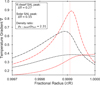 |
Fig. 8 Temperature gradients in the super-adiabatic layer (SAL) of a K dwarf (black) and solar model (red). The dashed and dot-dashed lines show the adiabatic gradient ∇ad and the structural gradient ∇, respectively. The vertical dashed lines indicate the radial location of the maximum difference between the gradients, and the diagnostic inserts presents the values of this difference along with the ratio of the local density at this point between the models. |
6.3 Granulation in a 3D K-dwarf simulation
To investigate this further we go beyond 1D stellar modelling and consider 3D hydrodynamic simulations of convection replicating the K-dwarf ε Indi A (Campante et al. 2024). The 1D stellar models showed that owing to a higher density in the exterior of K-dwarfs, a lower velocity is required to transport the required flux via convection, likely resulting in longer convective turnover times. If this inference holds, it should be corroborated by the 3D simulations where we have access to all details concerning the velocity flows of the convective elements.
Three simulations were calculated with the STAGGER code (Stein et al. 2024) using the solar abundances of Asplund et al. (2009) and targeted a Teff ≈ 4580 K and log (g)=4.62 dex, resulting in simulations of a MS star with vmax ≈ 5000 μHz. As done in Rodríguez Díaz et al. (2022) the resonance modes (box modes) of the simulation domain were damped. This was done by introducing an artificial damping timescale (as the inverse 1/ω of the cycling damping frequency) corresponding to half the frequency of the fundamental box mode, the frequency of the fundamental mode, and first overtone mode, respectively for each simulation. The horizontally averaged radiative flux was rescaled to the stellar surface following Trampedach et al. (1998) and Ludwig (2006) assuming the stellar radius of ε Indi A (Lundkvist et al. in prep.) for each simulation. The power spectra were then calculated as in Handberg & Campante (2011).
We applied the original framework of Larsen et al. (2025) to the power spectra of the simulations and recovered coherent results within the uncertainties for all three, suggesting that the choice of timescale for the artificial damping hardly affects our inferred parameters. The obtained timescales of the primary granulation component were then inspected and overplotted in Fig. 7 for the simulation with the longest damping timescale. Crucially, we find that the plateau in the granulation timescale is reproduced by the 3D simulations. The physical drivers in the stellar exteriors of K-dwarfs which result in longer timescales are thus present in our 3D simulations. This means that we can examine, in detail, what contributing factors play an important role in the convective behaviour of the K-dwarfs to produce the observed plateau.
To this end, we introduce two additional 3D simulations, one solar and one corresponding to an F-type dwarf. Their basic parameters are listed in Table 2, together with those of the simulation replicating ε-Indi. Recall that in a single-component model of granulation with exponent l=2, the parameter b is inversely proportional to the characteristic timescale of granulation, that is b=1 /(2 π tgran). The timescale, b, is tightly related to the typical size of the granules and the horizontal velocity at the optical surface. We estimated the granulation size similarly to Trampedach et al. (2013), where the 2D spatial power spectrum of bolometric intensity is computed for a series of simulation snapshots, followed by a radial average at different wave numbers. The peak of the time-averaged spatial spectrum indicates the typical size of granules. Next, we calculated the time-averaged distribution of horizontal velocity at the optical surface and selected the value with the highest probability to represent the characteristic surface horizontal velocity. The typical granulation timescale, tgran, is then crudely approximated as tgran ≈ dgran /(2 v̂h). All quantities for the three 3D simulations are tabulated in Table 2.
The typical granulation size quantified from the three 3D simulations is not far from the approximate scaling relation dgran ∝ Teff/g, due to its strong correlation with pressure scale height. However, when comparing horizontal velocities in the three simulations, we find a more pronounced decrease from the solar to the K-dwarf simulation than from the F-dwarf to solar, which implies that the granulation timescale increases more rapidly when moving from G- to F-type dwarfs. This is illustrated in Fig. 9, where the inverse of our estimated granulation timescale – which has a similar physical meaning as the parameter b− is plotted against vmax. Although the ‘plateau’ of 1 /(2 π tgran) from the solar position onwards is not as apparent as for the observations in Fig. 7, it is clear that the characteristic timescale of the granulation for the K-dwarf simulation t45g46m00 does not follow the expected functional form of the correlation between granulation and oscillation timescales.
The underlying reason for horizontal velocities decreasing more rapidly in K-dwarfs is likely associated with the fact that surface convection is much more efficient for cool dwarfs, as discussed in Sect. 6.2. 3D surface convection simulations suggest a moderate decrease of ∇−∇ad from F to G-type dwarfs, whereas the decrease of the gradient is notable for simulations with effective temperature less than ∼5500 K (cf. Fig. 25 of Magic et al. 2013), implying convection is much more efficient in K-dwarfs. A smaller super-adiabatic temperature gradient translates to weaker vertical and horizontal velocity fields. The change in the efficiency of convection across spectral types is well known from stellar models and manifests itself observationally in our detailed measurement of granulation timescales, as shown in Fig. 7.
Lastly, we note that stellar oscillations are excited predominantly by the vertical convective motions, in particular by the strong convective downdrafts near the stellar surface (Stein & Nordlund 2001). While we find a reduction in horizontal velocities for K-dwarfs affecting the granulation timescales, the location of the oscillation envelope and vmax remain consistent with expectations from asteroseismic scaling relations. This is consistent with vertical convective velocities relevant for mode excitation, i.e. the downdrafs, being comparatively unaffected (see e.g. Sect. 3.2.2 in Magic et al. 2013). As a result, the frequency separation between oscillation and granulation signals increases, as seen in the bottom panel of Fig. 2.
Basic properties of our 3D simulations.
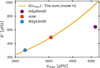 |
Fig. 9 Inverse of the granulation timescale, b′, plotted against the oscillation timescale vmax, estimated from the three 3D simulations listed in Table 2. We note that vmax was calculated using the asteroseismic scaling relation based on the fundamental parameters of the simulations. The gold solid line shows the fitted power law for model H from Fig. 6 with uncertainties indicated by the shaded bands, but scaled to pass the solar simulation. |
7 Conclusion
In this work we have further developed and applied the framework of Larsen et al. (2025) to the largest sample of short-cadence Kepler stars analysed to date, drawing on the catalogue by Sayeed et al. (2025). Our aim was to characterise the surface granulation signatures and assess the robustness and applicability of the background modelling framework across a diverse stellar population. We tested an alternative model description (peakbogging) for the power excess due to the presence of stellar oscillations, and while it shows promise, it requires additional work to remedy certain inconsistencies. Moving forwards with the traditional Gaussian envelope description, the following conclusions were reached:
Considering the background model preferences using the Bayesian evidences clearly shows no justification for a priori selection of background models. Rather, by applying a selection of models and choosing the one which best describes the given dataset, one allows for the optimal description of the background profile on a star-by-star basis.
The inferred value of vmax is sensitive to model misspecification. The formal uncertainties on vmax are often comparable to or dominated by the systematic uncertainty stemming from the choice of background description. This underlines that reliable oscillation-based inferences require careful treatment of the granulation signal.
The width of the Gaussian oscillation excess scales with vmax and indicates a temperature dependence. The dataset contributed by this work enables future studies of the correlations between envelope widths and various stellar parameters.
Total granulation amplitudes are consistent across background prescriptions and broadly align with the scaling relations of Kallinger et al. (2014) for evolved stars.
The observed characteristic frequency of the primary granulation component shows a decoupling with the oscillation timescale vmax for MS stars cooler than the Sun (vmax ≳ 3000 μHz) – indicating a plateau of prolonged granulation timescales for K-dwarfs.
The efficiency of the convective energy transport of K-dwarfs was examined by comparing 1D stellar models of Kepler-444 and the Sun. Due to the larger density in K-dwarf envelopes, and aided by a reduced luminosity, a lower velocity of the convective elements is necessary to transport the required flux. This leads to a smaller super-adiabatic temperature gradient and prolonged convective turnover times.
Using 3D hydrodynamical simulations of convection, we replicated the K-dwarf ε Indi A with vmax ≈ 5000 μHz and applied the background inference framework of Larsen et al. (2025) to the resulting power spectra. The 3D simulations reproduce the observed decoupling, reinforcing the physical picture supplied by the 1D stellar models.
The explanation for the decoupling likely stems from the much more efficient convective energy transport in K-dwarfs. The reduced super-adiabatic temperature gradients leads to weaker velocity fields, which from G- to K-dwarfs shows a significant decrease in the horizontal velocities, manifesting itself as prolonged granulation timescales in observations.
As a direct consequence of this decoupling, the scaling relations often adopted from Kallinger et al. (2014) for describing the granulation signal of dwarfs are shown not to hold for MS stars with vmax ≳ 3000 μHz. A fact which one should be aware of when, for example, simulations of power spectra for the upcoming ESA PLATO mission are made (Samadi et al. 2019; Rauer et al. 2025). Furthermore, this decoupling between granulation and oscillation timescales may offer a positive prospect for future detectability of asteroseismic signals in K-dwarfs, as it implies an increased frequency separation between the primary granulation signal and the oscillation excess. Moreover, it is noteworthy that the onset of the decoupling and the associated plateau in granulation timescales roughly coincides with the point where Campante et al. (2024) and Li et al. (2025) observed a deviation from the expected oscillation amplitude scaling – finding an apparent transition with decreasing L/M from a scaling of ∼(L/M)0.7 for the mode amplitudes to a steeper ∼(L/M)1.5 for K-dwarfs. As both the granulation and oscillations are fundamentally tied to the convective motions of the star, a decrease in the convective velocities would influence the excitation mechanism of the oscillations, suggesting that the two observed effects may share a common origin. However, other factors, such as mode damping, is also an important contribution, and it will require dedicated future studies to disentangle their roles and pinpoint the exact causes. Such efforts will represent an important step towards refining asteroseismic inferences and general stellar characterisation of K-dwarfs on the lower MS.
Alongside these physical insights, this work provides a comprehensive dataset: complete posterior distributions, parameter covariances, and Bayesian evidences for three background descriptions applied to 749 stars. When combined with the catalogue of Sayeed et al. (2025), the majority of them are also asteroseismically characterised, which provides estimates for the fundamental stellar parameters. This combination enables extensive future studies into how the surface signatures of convection ties to the stellar parameters across a diverse sample of stars spanning the MS, SGB and lower RGB.
Data availability
All data products for the 753 Kepler short-cadence stars studied are available in this online repository: https://www.erda.au.dk/archives/7edd1841b91dec2afd027a4bb7be3598/published-archive.html. The framework for the background inference is accessible on Github upon reasonable request to the first author, as it is currently under further development.
Acknowledgements
J.R.L. wishes to thank the members of SAC in Aarhus and the Sun, Stars and Exoplanets group in Birmingham for comments and discussions regarding the paper – in particular Jørgen Christensen-Dalsgaard and Hans Kjeldsen for helpful insights concerning stellar convection and thermodynamics. Additionally, the authors thank Maryum Sayeed for allowing us preliminary access to the catalogue data. This work was supported by a research grant (42101) from VILLUM FONDEN. M.S.L. acknowledges support from The Independent Research Fund Denmark’s Inge Lehmann program (grant agreement no.: 1131-00014B). M.N.L. acknowledges support from the ESA PRODEX programme (PEA 4000142995). Y.Z. acknowledges support from the European Union’s Horizon 2020 research and innovation programme under the Marie Skłodowska-Curie grant agreement No 101150921. Funding for the Stellar Astrophysics Centre was provided by The Danish National Research Foundation (grant agreement no.: DNRF106). The numerical results presented in this work were partly obtained at the Centre for Scientific Computing, Aarhus https://phys.au.dk/forskning/faciliteter/cscaa/. This paper received funding from the European Research Council (ERC) under the European Union’s Horizon 2020 research and innovation programme (CartographY GA. 804752). This paper includes data collected by the Kepler and TESS missions and obtained from the MAST data archive at the Space Telescope Science Institute (STScI). Funding for the Kepler mission was provided by the NASA Science Mission Directorate. Funding for the TESS mission is provided by the NASA Explorer Program. STScI is operated by the Association of Universities for Research in Astronomy, Inc., under NASA contract NAS 5-26555. This work presents results from the European Space Agency (ESA) space mission Gaia. Gaia data are being processed by the Gaia Data Processing and Analysis Consortium (DPAC). Funding for the DPAC is provided by national institutions, in particular the institutions participating in the Gaia MultiLateral Agreement (MLA). The Gaia mission website is https://www.cosmos.esa.int/gaia. The Gaia archive website is https://archives.esac.esa.int/gaia.
References
- Anderson, E. R., Duvall, Thomas L., J., & Jefferies, S. M. 1990, ApJ, 364, 699 [NASA ADS] [CrossRef] [Google Scholar]
- Appourchaux, T., 2004, A&A, 428, 1039 [NASA ADS] [CrossRef] [EDP Sciences] [Google Scholar]
- Asplund, M., Grevesse, N., Sauval, A. J., & Scott, P., 2009, ARA&A, 47, 481 [CrossRef] [Google Scholar]
- Ballot, J., Barban, C., & van’t Veer-Menneret, C., 2011, A&A, 531, A124 [NASA ADS] [CrossRef] [EDP Sciences] [Google Scholar]
- Bedding, T. R., 2014, in Asteroseismology, eds. P. L. Pallé, & C. Esteban (Berlin: Springer), 60 [Google Scholar]
- Böhm-Vitense, E., 1958, ZAp, 46, 108 [NASA ADS] [Google Scholar]
- Borucki, W. J., Koch, D., Basri, G., et al. 2010, Science, 327, 977 [Google Scholar]
- Campante, T. L., Barclay, T., Swift, J. J., et al. 2015, ApJ, 799, 170 [Google Scholar]
- Campante, T. L., Kjeldsen, H., Li, Y., et al. 2024, A&A, 683, L16 [NASA ADS] [CrossRef] [EDP Sciences] [Google Scholar]
- Chaplin, W. J., Kjeldsen, H., Bedding, T. R., et al. 2011, ApJ, 732, 54 [CrossRef] [Google Scholar]
- Chontos, A., Sayeed, M., & Huber, D., 2021, in Posters from the TESS Science Conference II (TSC2), 189 [Google Scholar]
- Corsaro, E., & De Ridder, J., 2014, A&A, 571, A71 [NASA ADS] [CrossRef] [EDP Sciences] [Google Scholar]
- Corsaro, E., Mathur, S., García, R. A., et al. 2017, A&A, 605, A3 [NASA ADS] [CrossRef] [EDP Sciences] [Google Scholar]
- Creevey, O. L., Sordo, R., Pailler, F., et al. 2023, A&A, 674, A26 [NASA ADS] [CrossRef] [EDP Sciences] [Google Scholar]
- Fröhlich, C., Romero, J., Roth, H., et al. 1995, Sol. Phys., 162, 101 [Google Scholar]
- Gaia Collaboration (Vallenari, A., et al.,) 2023, A&A, 674, A1 [NASA ADS] [CrossRef] [EDP Sciences] [Google Scholar]
- Gizon, L., & Solanki, S. K., 2003, ApJ, 589, 1009 [Google Scholar]
- Handberg, R., & Campante, T. L., 2011, A&A, 527, A56 [CrossRef] [EDP Sciences] [Google Scholar]
- Handberg, R., & Lund, M. N., 2014, MNRAS, 445, 2698 [Google Scholar]
- Handberg, R., Brogaard, K., Miglio, A., et al. 2017, MNRAS, 472, 979 [CrossRef] [Google Scholar]
- Harvey, J., 1985, ESA SP, 235, 199 [Google Scholar]
- Hekker, S., Kallinger, T., Baudin, F., et al. 2009, A&A, 506, 465 [NASA ADS] [CrossRef] [EDP Sciences] [Google Scholar]
- Hon, M., Huber, D., Li, Y., et al. 2024, ApJ, 975, 147 [Google Scholar]
- Huber, D., Stello, D., Bedding, T. R., et al. 2009, Commun. Asteroseismol., 160, 74 [Google Scholar]
- Huber, D., Bedding, T. R., Stello, D., et al. 2011, ApJ, 743, 143 [Google Scholar]
- Johnson, N. L., Kotz, S., & Balakrishnan, N., 1995, Continuous Univariate Distributions, 2nd edn., Wiley Series in Probability and Statistics (New York: John Wiley & Sons), 2, 752 [Google Scholar]
- Kallinger, T., De Ridder, J., Hekker, S., et al. 2014, A&A, 570, A41 [NASA ADS] [CrossRef] [EDP Sciences] [Google Scholar]
- Karoff, C., Campante, T. L., Ballot, J., et al. 2013, ApJ, 767, 34 [Google Scholar]
- Kim, K.-B., & Chang, H.-Y., 2021, New A, 84, 101522 [Google Scholar]
- Kippenhahn, R., Weigert, A., & Weiss, A., 2013, Stellar Structure and Evolution (Berlin: Springer) [Google Scholar]
- Kjeldsen, H., & Bedding, T. R., 1995, A&A, 293, 87 [NASA ADS] [Google Scholar]
- Kjeldsen, H., & Bedding, T. R., 2011, A&A, 529, L8 [NASA ADS] [CrossRef] [EDP Sciences] [Google Scholar]
- Laplace, P., 1812, Théorie Analytique Des Probabilités (Paris: Courcier) [Google Scholar]
- Larsen, J. R., Lundkvist, M. S., Davies, G. R., et al. 2025, A&A, 701, A92 [NASA ADS] [CrossRef] [EDP Sciences] [Google Scholar]
- Li, Y., Huber, D., Ong, J. M. J., et al. 2025, ApJ, 984, 125 [Google Scholar]
- Lightkurve Collaboration (Cardoso, J. V. d. M., et al.) 2018, Astrophysics Source Code Library [record ascl:1812.013] [Google Scholar]
- Llorente, F., Martino, L., Curbelo, E., López-Santiago, J., & Delgado, D., 2023, WIREs Comput. Statis., 15, e1595 [Google Scholar]
- Ludwig, H. G., 2006, A&A, 445, 661 [NASA ADS] [CrossRef] [EDP Sciences] [Google Scholar]
- Lund, M. N., Handberg, R., Davies, G. R., Chaplin, W. J., & Jones, C. D., 2015, ApJ, 806, 30 [NASA ADS] [CrossRef] [Google Scholar]
- Lund, M. N., Silva Aguirre, V., Davies, G. R., et al. 2017, ApJ, 835, 172 [Google Scholar]
- Lund, M. N., Chontos, A., Grundahl, F., et al. 2025, A&A, 701, A285 [NASA ADS] [CrossRef] [EDP Sciences] [Google Scholar]
- Lundkvist, M. S., Ludwig, H.-G., Collet, R., & Straus, T., 2021, MNRAS, 501, 2512 [CrossRef] [Google Scholar]
- Lundkvist, M. S., Kjeldsen, H., Bedding, T. R., et al. 2024, ApJ, 964, 110 [NASA ADS] [CrossRef] [Google Scholar]
- Magic, Z., Collet, R., Asplund, M., et al. 2013, A&A, 557, A26 [NASA ADS] [CrossRef] [EDP Sciences] [Google Scholar]
- Mathur, S., Hekker, S., Trampedach, R., et al. 2011, ApJ, 741, 119 [Google Scholar]
- Michel, E., Samadi, R., Baudin, F., et al. 2009, A&A, 495, 979 [NASA ADS] [CrossRef] [EDP Sciences] [Google Scholar]
- Mosser, B., Elsworth, Y., Hekker, S., et al. 2012, A&A, 537, A30 [NASA ADS] [CrossRef] [EDP Sciences] [Google Scholar]
- Nielsen, M. B., Davies, G. R., Ball, W. H., et al. 2021, AJ, 161, 62 [NASA ADS] [CrossRef] [Google Scholar]
- Nielsen, M. B., Ong, J. M. J., Hatt, E. J., et al. 2025, AJ, 169, 322 [Google Scholar]
- Ramírez, I., Allende Prieto, C., & Lambert, D. L., 2013, ApJ, 764, 78 [CrossRef] [Google Scholar]
- Rauer, H., Aerts, C., Cabrera, J., et al. 2025, Exp. Astron., 59, 26 [Google Scholar]
- Ricker, G. R., Winn, J. N., Vanderspek, R., et al. 2014, SPIE Conf. Ser., 9143, 914320 [Google Scholar]
- Rodríguez Díaz, L. F., Bigot, L., Aguirre Børsen-Koch, V., et al. 2022, MNRAS, 514, 1741 [CrossRef] [Google Scholar]
- Samadi, R., Belkacem, K., Ludwig, H. G., et al. 2013, A&A, 559, A40 [NASA ADS] [CrossRef] [EDP Sciences] [Google Scholar]
- Samadi, R., Deru, A., Reese, D., et al. 2019, A&A, 624, A117 [NASA ADS] [CrossRef] [EDP Sciences] [Google Scholar]
- Santos, A. R. G., Godoy-Rivera, D., Finley, A. J., et al. 2024, Front. Astron. Space Sci., 11, 1356379 [NASA ADS] [CrossRef] [Google Scholar]
- Sayeed, M., Huber, D., Chontos, A., & Li, Y., 2025, AJ, 170, 212 [Google Scholar]
- Schofield, M., 2019, Phd thesis (University of Birmingham, UK) [Google Scholar]
- Serenelli, A., Johnson, J., Huber, D., et al. 2017, ApJS, 233, 23 [Google Scholar]
- Silva Aguirre, V., Davies, G. R., Basu, S., et al. 2015, MNRAS, 452, 2127 [Google Scholar]
- Speagle, J. S., 2020, MNRAS, 493, 3132 [Google Scholar]
- Sreenivas, K. R., Bedding, T. R., Li, Y., et al. 2024, MNRAS, 530, 3477 [NASA ADS] [CrossRef] [Google Scholar]
- Stein, R. F., & Nordlund, Å. 2001, ApJ, 546, 585 [Google Scholar]
- Stein, R. F., Nordlund, Å., Collet, R., & Trampedach, R. 2024, ApJ, 970, 24 [NASA ADS] [CrossRef] [Google Scholar]
- Stello, D., Chaplin, W. J., Basu, S., Elsworth, Y., & Bedding, T. R., 2009a, MNRAS, 400, L80 [Google Scholar]
- Stello, D., Chaplin, W. J., Bruntt, H., et al. 2009b, ApJ, 700, 1589 [NASA ADS] [CrossRef] [Google Scholar]
- Themeßl, N., Kuszlewicz, J. S., García Saravia Ortiz de Montellano, A., & Hekker, S. 2020, in Stars and their Variability Observed from Space, eds. C. Neiner, W. W. Weiss, D. Baade, R. E. Griffin, C. C. Lovekin, & A. F. J. Moffat (Australia: University of Vienna), 287 [Google Scholar]
- Trampedach, R., Christensen-Dalsgaard, J., Nordlund, A., & Stein, R. F., 1998, in The First MONS Workshop: Science with a Small Space Telescope, eds. H., Kjeldsen, & T. R. Bedding (USA: APA), 59 [Google Scholar]
- Trampedach, R., Asplund, M., Collet, R., Nordlund, Å., & Stein, R. F. 2013, ApJ, 769, 18 [NASA ADS] [CrossRef] [Google Scholar]
- Van Cleve, J. E., Christiansen, J. L., Jenkins, J. M., et al. 2016, Kepler Data Characteristics Handbook, KSCI-19040-005, eds. D. Caldwell, J. M. Jenkins, M. R. Haas, & N. Batalha (USA: Kepler Science Document), 2 [Google Scholar]
- Weiss, A., & Schlattl, H., 2008, Ap&SS, 316, 99 [CrossRef] [Google Scholar]
- Winther, M. L., Aguirre Børsen-Koch, V., Rørsted, J. L., Stokholm, A., & Verma, K., 2023, MNRAS, 525, 1416 [NASA ADS] [CrossRef] [Google Scholar]
- Yu, J., Huber, D., Bedding, T. R., et al. 2018, ApJS, 236, 42 [NASA ADS] [CrossRef] [Google Scholar]
- Zhou, Y., Nordlander, T., Casagrande, L., et al. 2021, MNRAS, 503, 13 [NASA ADS] [CrossRef] [Google Scholar]
Appendix A Specific removals from sample
This appendix contains Table A.1 which specifies the 12 stars that were removed from the Sayeed et al. (2025) catalogue, along with the reasons why.
Specific stars removed from the Sayeed et al. (2025) catalogue with the reasons noted.
Appendix B Prior densities in model selection
This appendix briefly discusses the considerations underlying our choice of prior densities. A comprehensive treatment of the associated challenges and caveats can be found in Llorente et al. (2023). In this work, we are concerned with addressing two related but distinct inference problems. The first is to determine the optimal parameters θ of a given model M that best describe a set of data D – what Llorente et al. (2023) refer to as a level-1 inference. In such cases, if no strong prior knowledge is available, non-informative priors (e.g. uniform distributions spanning the entire parameter space) provide an objective starting point. These allow the nested sampler to explore the full parameter space and identify the optimal set of θ values, albeit often at the cost of slower convergence. The second problem is model selection, based on the Bayesian evidence (or marginal likelihood), which Llorente et al. (2023) classify as a level-2 inference. Here, the choice of priors directly influences the result and thereby our later interpretations. The evidence is given by
 (B.1)
From this expression, it is evident that the volume of the prior p(θ ∣ M) affects the evidence 𝒵. Broad or non-informative priors with large volumes reduce the evidence and thus penalise the corresponding model. We must be astutely aware of this fact when defining our priors, at the same time as ensuring that we define priors which allow for the optimal set of parameters θ to be recovered.
(B.1)
From this expression, it is evident that the volume of the prior p(θ ∣ M) affects the evidence 𝒵. Broad or non-informative priors with large volumes reduce the evidence and thus penalise the corresponding model. We must be astutely aware of this fact when defining our priors, at the same time as ensuring that we define priors which allow for the optimal set of parameters θ to be recovered.
This penalisation of large prior volumes is, however, an intended feature of the Bayesian framework. Models with a greater number of free parameters are naturally penalised unless those parameters substantially improve the likelihood p(D ∣ θ, M), thereby providing genuine explanatory power. Even so, it is essential to ensure that the priors are defined consistently across models to prevent unintended biases. For parameters common to multiple models – such as the first two Harvey components in models H and T – we therefore adopt priors with identical functional forms and boundaries broad enough to include the plausible ranges for all models. For parameters that are directly data-driven (e.g. the white-noise level), the priors are defined solely from the data and applied identically to all models, ensuring a fair contribution to Eq. B.1. The only exception is the amplitude parameter of model J, whose functional form differs fundamentally from those of models H and T. In this case, the prior’s central value is adjusted accordingly, while its functional form and scale remains identical (see Table C.1).
Appendix C Overview of priors
This appendix defines the priors adopted in this work. In Table C.1 the priors for the parameters of the granulation background models from Table 1 are presented. The priors for the general term parameters identical across granulation background models – which describe stellar activity, the oscillation excess, and white noise – are found in Table C.2, and are primarily defined based on the PDS data for the given star.
The model-specific priors in Table C.1 are presented for both the correlated-inference setup described in Sect. 3.1, which introduces the scatter parameters σa, b, d, and additionally also the case when all parameters are treated as free variables. For model J, whose functional form differs from that of models H and T, the amplitude parameter a is always inferred directly, and its prior follows the prescription of Larsen et al. (2025). In the correlated inference, a broader prior is used for the amplitude scatter parameter, implemented as a log-normal distribution, while the characteristic frequencies are constrained to lie within ± 40% of the values predicted by the scaling relations of Kallinger et al. (2014). This choice permits substantial deviation from the scaling relations, reflecting the fact that our sample consists primarily of short-cadence MS and SGB stars, whereas the relations of Kallinger et al. (2014) were derived for RGB stars. Thus, we use those relations only as general guidelines rather than strict prescriptions. Furthermore, especially when using the peakbogging approach described in Appendix. E, the framework is by construction entirely different to that of Kallinger et al. (2014). Thereby, the choices made for the priors of σa, b, d ensure that we do not unintentionally bias our results. Consistent with the discussion in Appendix B, we note that many of the priors listed in Table C.1 are identical across the granulation background models, ensuring fair and consistent treatment in the model comparison.
For completeness, we provide the functional forms of the beta and log-normal distributions used throughout this work. For parameters bounded within finite intervals, we employ beta distributions with probability density function:
 (C.1)
where x ∈[loc, loc+scale], B(a, b)=Γ(a) Γ(b)/Γ(a+b) is the beta function, and the shape parameters a, b>0 control the distribution’s concentration and skewness. The parameters loc and scale define the lower bound and width of the distribution, respectively. When data-driven priors are used, the shape parameters are determined via the mode-concentration relation a(m)=m(k−2)+1 and b(m)=(1−m)(k−2)+1 with concentration parameter k=10 and mode value m as specified from the data, ensuring the distribution peaks at the desired location (Johnson et al. 1995).
(C.1)
where x ∈[loc, loc+scale], B(a, b)=Γ(a) Γ(b)/Γ(a+b) is the beta function, and the shape parameters a, b>0 control the distribution’s concentration and skewness. The parameters loc and scale define the lower bound and width of the distribution, respectively. When data-driven priors are used, the shape parameters are determined via the mode-concentration relation a(m)=m(k−2)+1 and b(m)=(1−m)(k−2)+1 with concentration parameter k=10 and mode value m as specified from the data, ensuring the distribution peaks at the desired location (Johnson et al. 1995).
Compilation of the general priors for the complete background model terms describing stellar activity, the oscillation excess, and white noise.
For strictly positive parameters varying over orders of magnitude, we may adopt log-normal priors implemented by placing a normal distribution on the base-10 logarithm of the parameter:
 (C.2)
which corresponds to the probability density:
(C.2)
which corresponds to the probability density:
![Mathematical equation: $p(\theta \mid \mu, \sigma)=\frac{1}{\theta \ln (10) \sqrt{2 \pi} \sigma} \exp \left[-\frac{\left(\log _{10} \theta-\mu\right)^{2}}{2 \sigma^{2}}\right],$](/articles/aa/full_html/2026/03/aa58683-25/aa58683-25-eq59.png) (C.3)
for θ>0. Here, μ represents the centre of the prior on the logarithmic scale (corresponding to a median of 10μ in linear space), and σ controls the width, with typical values of σ=0.1 providing mild regularisation.
(C.3)
for θ>0. Here, μ represents the centre of the prior on the logarithmic scale (corresponding to a median of 10μ in linear space), and σ controls the width, with typical values of σ=0.1 providing mild regularisation.
Appendix D A TESS K-dwarf sample
In Sect. 5.2 we noted that the primary granulation timescale appears to plateau for cool MS stars (K dwarfs; Fig. 6), although this suggestion is based on only a modest number of objects. To reinforce this indication we sought additional K dwarfs beyond those observed by Kepler, turning to photometry from TESS (Ricker et al. 2014).
We did not expect the stars recovered to display clear oscillatory signatures. However, we required approximate vmax values both to guide our priors and to compare against the resulting granulation timescales. To obtain such an estimate, we used to the asteroseismic scaling relation (Kjeldsen & Bedding 1995):
 (D.1)
with vmax, ⊙=3090 μHz, g⊙=104.44 g cm−2, and Teff, ⊙= 5777 K. Thus we needed estimates for the surface gravities g and effective temperatures Teff for the sample stars. In order to form a sample of K-dwarfs most likely to display granulation in the TESS photometry, while also obtaining the above parameters, we turned to Gaia (Gaia Collaboration 2023).
(D.1)
with vmax, ⊙=3090 μHz, g⊙=104.44 g cm−2, and Teff, ⊙= 5777 K. Thus we needed estimates for the surface gravities g and effective temperatures Teff for the sample stars. In order to form a sample of K-dwarfs most likely to display granulation in the TESS photometry, while also obtaining the above parameters, we turned to Gaia (Gaia Collaboration 2023).
We queried the Gaia archive for bright, high-quality single stars consistent with K-dwarf temperatures and luminosities, imposing the following criteria:
mG<11
parallax >1 mas (d<1 kpc)
ruwe < 1.4
non_single_star = 0
phot_proc_mode = 0
phot_bp_rp_excess_factor ∈[0.5, 1.5]
bp_rp ∈ [0.9, 1.5]
MG ∈ [4.5, 7.0]
logg_gspphot >4.4 dex
Conditions 1-6 ensure bright, well-behaved single stars; conditions 7-9 restrict the selection to a broad K-dwarf region in colour-magnitude space and suitable surface gravities. We retrieved the top 200 stars sorted by apparent G magnitude. For each star we obtained the corresponding TIC ID via ExoFOP, and checked for available 20 s cadence TESS data through MAST using LightCurve (Lightkurve Collaboration 2018). When such data were available, we constructed a preliminary power density spectrum from the SPOC light curves for visual inspection of any tentative granulation signal present. This yielded an initial list of 72 candidates.
We supplemented this list with several known TESS K-dwarf candidate oscillators observed at 20 s cadence: TIC 283722336 (HD 219134), TIC 398120047 (70 Oph A), TIC 79454735 (36 Oph), TIC 389198736 (HD 191408), Furthermore, we also added the confirmed oscillators TIC 259237827 (σ Dra; Hon et al. 2024) and TIC 67772871 (40 Eri A; Lund et al. 2025), moreover noting that another known oscillator TIC 231698181 (ε Indi; Lundkvist et al. 2024; Campante et al. 2024) was already included in the Gaia-selected sample. For these additions we adopted Teff and log g from the TESS Input Catalog v8.2, except for TIC 79454735 and TIC 389198736 where the estimates were recovered from ExoFOP and Ramírez et al. (2013), respectively.
Altogether, we obtained 78 targets. For each, the TESS target pixel files were subsequently retrieved and custom aperture photometry was performed following Lund et al. (2015) and Lund et al. (2025) to construct the light curves. Power density spectra were then computed following Handberg & Campante (2011).
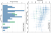 |
Fig. D.1 Kiel diagram and vmax distribution of the TESS K-dwarf sample. The initial list obtained through the Gaia query and TESS 20 second cadence overlap is shown in blue, while the manual additions are indicated in green. |
Appendix D.1 The resulting sample
The Gaia gspphot parameters for the selected stars pass stringent quality filters and are suitable for estimating vmax for our purposes (Creevey et al. 2023). Because the formal (internal) Gaia uncertainties are unrealistically small, we adopted conservative values of σTeff=150 K and σlog g=0.05 dex for all stars, which propagate to uncertainties of roughly 360−600 μHz in vmax. For the additional targets drawn from the TIC, the quoted log g uncertainties can approach 0.1 dex, yielding vmax errors of order 1000 μHz. Since vmax serves only to guide prior placement and to indicate the approximate position of each star on the potential timescale plateau, these uncertainties are acceptable. For σ Dra and ε Indi we directly adopt the published vmax values and uncertainties from Hon et al. (2024) and Campante et al. (2024), respectively.
The final TESS K-dwarf sample is shown in Fig. D.1. Despite the sizeable uncertainties – particularly in the surface gravity the stars broadly trace the expected lower MS trend in the Kiel diagram. The resulting vmax estimates span the desired range, from slightly above the solar value up to just beyond 5000 μHz.
Appendix E Peakbogging
The assumption of a Gaussian oscillation excess means overlaying an entire envelope to describe the power arising from the stellar oscillations. Yet, as described previously, the power contained in the narrow Lorentzian peaks is not well represented by a smooth Gaussian excess. The most realistic description would be to individually model the observed frequencies as each their own Lorentzian excess, colloquially known as ‘peakbagging’, which is used extensively when performing mode identification of seismic targets (see e.g. Corsaro & De Ridder 2014; Themeßl et al. 2020; Nielsen et al. 2021; Nielsen et al. 2025). This is, however, a very complex process with many nuances in the chosen treatment of the stellar pulsations as a function of evolution, furthermore affected by phenomena such as rotation, binarity, and magnetic fields. In the present work we aim for a middle ground: to go beyond a Gaussian envelope without having to individually model the stellar oscillations. This is because our interest is in the underlying stellar granulation background and not the oscillations themselves. We wish to essentially treat the power contained in the peaks as noise standing on top of the background. For this purpose we present peakbogging, which is a methodology that uses a mixture model for the likelihood during the inference of the background model.
Appendix E.1 A mixture-model likelihood setup
The likelihood function ℒ is identical to that used for the Gaussian approach as specified in Eq. 1. Peakbogging uses a mixture-model likelihood function for the inference, which is the sum of a foreground and background contribution,
 (E.1)
Here, M denotes the given background model, β is a free scaling parameter, and G(v, θ) is the mixture coefficient assumed to be Gaussian with parameters θ. The definition of the background and foreground contributions are in essence quite simple, while it is the interplay between them during sampling that becomes complex. The first term in Eq. E.1 containing ℒ1 is the background contribution and contains the pure model from Table 1 assumed to describe the granulation background signal. The latter term containing ℒ2 is the foreground contribution which serves the purpose of absorbing any excess in power not predicted by the assumed background model, which it may do by amplifying the predicted power of the background model by the scaling factor β.
(E.1)
Here, M denotes the given background model, β is a free scaling parameter, and G(v, θ) is the mixture coefficient assumed to be Gaussian with parameters θ. The definition of the background and foreground contributions are in essence quite simple, while it is the interplay between them during sampling that becomes complex. The first term in Eq. E.1 containing ℒ1 is the background contribution and contains the pure model from Table 1 assumed to describe the granulation background signal. The latter term containing ℒ2 is the foreground contribution which serves the purpose of absorbing any excess in power not predicted by the assumed background model, which it may do by amplifying the predicted power of the background model by the scaling factor β.
Notably, the assumed background model M for the granulation signal is present in both the foreground and background contributions. This means that even in regions where the foreground plays a significant role, there is still some sensitivity to the background model and the parameters it contains (such as granulation amplitudes and timescales). In summary, the aim of peakbogging is thus to allow the background model parameters to be determined given the possibility of excess power being present in a certain frequency bin, which is absorbed to avoid unwanted perturbation of the background model inference.
Appendix E.2 The mixture coefficient for control
To construct the mixture model, we introduce the Gaussian mixture coefficient G(v, θ), which regulates the relative contribution of the foreground and background components as a function of frequency. Its formulation allows explicit control over the frequency range where the foreground model is permitted to influence the likelihood. The coefficient is defined as a Gaussian function normalised between 0 and 1,
![Mathematical equation: $G(v, \theta)=H \exp \left[-\frac{\left(v-v_{\max}\right)^{2}}{2 \sigma^{2}}\right],$](/articles/aa/full_html/2026/03/aa58683-25/aa58683-25-eq62.png) (E.2)
where H denotes the height of the Gaussian and thus the strength of the foreground contribution. In practice, H may be interpreted as a measure of the probability that excess power is present beyond what is predicted by the background model (i.e. ‘peakbog detection probability’) – hence, H>0 indicates the detection of such an excess. The centroid vmax identifies the frequency around which the foreground component becomes active, corresponding to the region where most of the excess power resides. When no significant artefacts affect the PDS and the oscillations are well resolved, this centroid is roughly expected to coincide with vmax from the traditional Gaussian envelope description. Furthermore, we anticipate that the determination of vmax in the peakbogging approach may be less sensitive to model misspecification; a suspicion that we will be examined further in Appendix E.5.2
(E.2)
where H denotes the height of the Gaussian and thus the strength of the foreground contribution. In practice, H may be interpreted as a measure of the probability that excess power is present beyond what is predicted by the background model (i.e. ‘peakbog detection probability’) – hence, H>0 indicates the detection of such an excess. The centroid vmax identifies the frequency around which the foreground component becomes active, corresponding to the region where most of the excess power resides. When no significant artefacts affect the PDS and the oscillations are well resolved, this centroid is roughly expected to coincide with vmax from the traditional Gaussian envelope description. Furthermore, we anticipate that the determination of vmax in the peakbogging approach may be less sensitive to model misspecification; a suspicion that we will be examined further in Appendix E.5.2
Lastly, we have the standard deviation of the Gaussian σ which controls the size of the region where the foreground model is significant. Importantly, σ is not allowed to vary freely during the inference. We reinterpret the mixture coefficient width σ not as a parameter to be inferred, but as a prior-informed localisation term that reflects the expected region of the oscillation excess. This approach prevents the mixture model from becoming sensitive to spurious features across the spectrum and ensures that the foreground model is only applied in a physically meaningful domain. For a given star, we use the estimate for the FWHM of the oscillation excess from Mosser et al. (2012) to inform the width:
 (E.3)
We make the conservative choice to enhance the width of the mixture coefficient to be larger than expected by a factor of 1.5, while the factor
(E.3)
We make the conservative choice to enhance the width of the mixture coefficient to be larger than expected by a factor of 1.5, while the factor  converts the FWHM to the width σ. Crucially, as we use a Gaussian mixture coefficient, non-zero tails exist throughout the spectrum. Hence, if there, for example, exists a strong systematic peak in the PDS – which is not described by the background model – the large difference in the log-likelihood probability between the foreground and background contributions of Eq. E.1 will still allow for peakbogging to take effect.
Appendix E.3 Binning for peakbogging
In Sect. 3.2 it was discussed how moderately binning the data was beneficial and did not affect the inference for the traditional Gaussian approach. For peakbogging, binning is essential as it enhances the contrast between the granulation background and contaminating signals, whether from stellar oscillations or otherwise. Since peakbogging models the oscillation contributions through a flexible likelihood mixture component able to absorb signal not described by the assumed background, unbinned data can lead the sampler to confuse stochastic noise peaks with genuine pulsation power, causing the mixture model to overestimate the foreground contribution. When this happens, the granulation parameters are biased downwards, i.e. the model component(s) accounts for less overall power, which in turn makes it even easier for the mixture model to continue absorbing the true signal during subsequent sampling steps. Moderate binning mitigates this instability by reducing the prominence of spurious peaks.
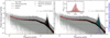 |
Fig. E.1 Background fits for the Sun using a Gaussian envelope (left) and peakbogging (right). A two-component Harvey model (H) is used for the inference on the PDS of a ∼3.15 year time series of VIRGO (Fröhlich et al. 1995) blue band data taken during the solar minimum between cycle 23 and 24. Left: the unbinned PDS shown in grey and the binned version is overplotted in black. The model is plotted in red using the median of the obtained posteriors for each fit parameter. Additionally, 50 randomly drawn samples from the posteriors are plotted to indicate the scatter. The individual granulation components are plotted as dashed green profiles. The fitted value of vmax is given and indicated by the vertical dashed black line, while the noise is shown by the horizontal dashed orange line. The activity component is the dash-dotted green line. The model without the influence of the Gaussian oscillation excess is plotted as the dashed blue profile, visible underneath the oscillation excess. Right: same as left, but the Gaussian mixture coefficient controlling the peakbog mixture-model likelihood in Eq. E.1 is plotted as the blue profile, with the secondary y-axis showing the amplitude, H. Whenever log (ℒforeground−ℒbackground)>2, the data is coloured cyan to indicate the dominance of the foreground contribution in the peakbogging. The insert shows the log-likelihood ratio between the foreground and background contributions of the mixture model in a region around vmax. |
For the three stars considered in the main article – KIC 6679371, KIC 8866102, and KIC 8006161 – no change was found as a function of binning for the Gaussian approach. In contrast, for the peakbogging approach, nuances occur at low degrees of binning (i.e. high frequency resolution) which vary from star to star, but common to all is that they converge as the binning becomes moderate. When the bin size reflects a frequency resolution larger than ∼0.3 μHz (conservative boundary), further increasing the bin size causes negligible changes. As was argued in Sect. 3.2 we bin to a resolution of 0.5 μHz if the time series duration allows, which is above this boundary. The nuances of how peakbogging is sensitive to the binning is displeasing and points towards the challenges of constraining a model with significantly more freedom during the statistical inference.
Appendix E.4 Peakbogging the Sun
In order to visualise the nature of peakbogging and its different aspects, Fig. E.1 shows the background model inference with a two-component Harvey model (see model H in Table 1) for the Sun when employing a Gaussian envelope vs. peakbogging. Given the insert of Fig. E.1 we can inspect the log-likelihood ratio between the foreground and background contributions of Eq. E.1, and visually see which peaks have been absorbed by the peakbogging. We see that for the Sun, the foreground contribution dominates in a wide region around the observed vmax as desired. Contrary to the traditional method with a Gaussian envelope for the oscillation excess, which presents as a ‘bump’ on top of the background-only profile, we see the peakbogged data standing in discrete peaks on top of the background model.
The vmax obtained from the two approaches have some conceptual differences to be aware of. The Gaussian envelope provides an estimate of vmax which connects to literature (Bedding 2014) as the centroid of the distribution. The peakbogging does not, however, estimate its corresponding vmax as the centre of the stellar oscillations in frequency, but rather as the centre of a Gaussian mixture coefficient describing the probability for excess signal. The resulting estimate of vmax ought to be closely related and both suffer from generalities, i.e. they are both generated from the data but lack rigour, both suffer from model misspecification, and both will need effort concerning systematic corrections when referenced to models of stellar evolution. For this specific case, this difference means a shift from  for the Gaussian case to
  when peakbogging is used.
In Appendix E.2 the setup of peakbogging using a predefined and locked width of the mixture coefficient was discussed, and how despite this choice, a clear preference for the foreground contribution may lead to it dominating at a location displaced from vmax. This situation, however, is not showcased in Fig. E.1. However, although the log-likelihood ratio in the insert is below 0, reflecting preference for the pure background, peakboggin was allowed to asses the entire PDS for potential excess signal. Peakbogging should thereby be widely applicable when dealing with excess signal not described by the assumed model, be it instrumental peaks or potentially rotational peaks at low frequencies. If and how such peaks affect the vmax determination, however, is uncertain and has not been studied in this context. A proper approach may be to implement three terms into the mixture-model, such that you have an oscillation absorber and instrumental and/or rotation absorber, acting in isolation from each other in different regions of the PDS.
For the case of the Sun presented here, the difference between using the traditional Gaussian envelope and peakbogging is most clearly seen in the second granulation component. For the Gaussian case the characteristic frequency,  , which roughly indicates the position of the knee in the component, lies above the determined vmax. It is thus shifted towards higher frequency than would be expected (Karoff et al. 2013), possibly because the sampler absorbs some of the power of the oscillation excess into the granulation component. In contrary, when using the peakbogging setup
  lies below the determined νmax, and the corresponding component amplitude c is lowered accordingly – which follows the expectations from Karoff et al. (2013) and Kallinger et al. (2014) almost exactly. Note that these nuances may differ when considering alternate background models, and in this context simply indicates the difference in behaviour and potential benefits of using the peakbogging approach. Yet, the presented example is for the unique case of the Sun, and we will now discuss the application and limitations of peakbogging when applied to the entire sample of stars studied in this work.
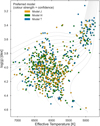 |
Fig. E.2 Kiel diagram with colouring according to normalised evidence ratios, with model preferences as indicated by the legend. When models are comparable in their evidences the colour is blended between the two competing models. The Sun is overplotted as the enlarged star symbol at the solar location and significantly prefers model T. |
Appendix E.5 Background model preferences and sensitivities for peakbogging
For the remainder of this appendix, we now largely follow the approach of the main article. In this section we thus evaluate the background model preferences and sensitivities, before considering the granulation parameters themselves in Appendix E.6. For peakbogging a total of 7 stars failed to produce meaningful posteriors during the inference and were therefore discarded, resulting in a sample of 746 stars.
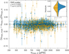 |
Fig. E.3 Comparison of the vmax determination across the different models. The vmax fractional residuals of models J and T to those obtained by model H are plotted in yellow and blue, respectively. The horizontal dashed line indicates perfect agreement in vmax determinations, while the dot-dashed show the 2% bounds. The RMS scatter was calculated for both cases and is provided in the inserted box in the top left. The insert shows a split violin plot of the vmax residual distributions for model J (left) and model T (right) versus model H, with medians and 16th/84th percentiles overplotted as full and dashed horizontal lines, respectively. |
Appendix E.5.1 Background model preferences
In Fig. E.2 we see the evidence ratios obtained when using the peakbogging approach. There is a clear difference in the model preferences, namely that the hybrid model J is preferred in far more cases than for the Gaussian approach (see Sect. 4 and Fig. 3). For peakbogging, the number of stars preferring each background model of Table 1 is split roughly into thirds, showing no overall preference or trend in the Kiel diagram. Due to the clear differences between what was obtained with the Gaussian approach, we see how the implemented model for the oscillation excess directly affects the model preferences. This was our initially worry as well as motivation for testing an alternative approach to the traditional Gaussian envelope approach.
Thus, when considering the changes between Figs. 3 and E.2, we see how the optimal model for describing the stellar data is sensitive to our setup and associated assumptions. This provides further emphasis for the arguments presented by Handberg et al. (2017), namely that one should not a priori fix the background model, but rather assess which model best describes the given dataset.
Appendix E.5.2 Background model sensitivity of vmax
In Appendix E.2 we discussed how peakbogging may be less sensitive to model misspecification. Figure E.3 shows the vmax residuals akin to those shown in Fig. 4 for the Gaussian approach. There are two things to note: 1) the RMS is actually slightly larger than that obtained by the Gaussian approach, meaning we do not see a reduction in sensitivity to the choice of background model, and 2), the formal uncertainties of vmax obtained through peakbogging are larger.
Contrary to the Gaussian approach, we find somewhat less clear systematics in the obtained residuals, and since the formal uncertainties are larger they better explain the observed scatter – for both comparisons with model H the uncertainties are consistent with zero 96% of the time. Generally it thus seems that the peakbogging approach returns more realistic uncertainties on vmax when implemented into our framework, in comparison to what the simplistic and constrained Gaussian model obtains.
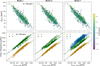 |
Fig. E.4 Total granulation amplitudes and characteristic frequencies as a function of vmax obtained by the three background models of Table 1. In all panels, the dashed lines represent the corresponding scaling relation for the parameter from Kallinger et al. (2014). Top row: total granulation amplitudes colour-coded by the stellar metallicity [Fe/H] for the 724 stars with available temperatures. Bottom row: the characteristic frequencies of the individual granulation components for the 746 stars with consistent posteriors, with colours as indicated by the legend. |
Appendix E.6 Scaling of granulation parameters for peakbogging
Figure E.4 presents the total granulation amplitudes and characteristic frequencies obtained for the sample using the peakbogging approach. We have chosen not to fit power laws to determine scaling relations in the case of peakbogging, as certain pathologies which plague peakbogging will become evident in the subsequent discussion.
The total granulation amplitudes are largely identical to those predicted by the Gaussian approach in Fig. 6. This is a redeeming result for peakbogging, since the approaches vary significantly but the total power attributed to the granulation remains consistent. Moreover, the amplitudes also follow those predicted by Kallinger et al. (2014). The primary granulation timescale across the three background models behave similarly for peakbogging as it did for the Gaussian approach. We still notice some systematic differences to the scaling relation of Kallinger et al. (2014). Crucially, the departure from the strict correlation between the granulation and oscillation timescale is also recovered by peakbogging, seen as the apparent formation of the plateau in the timescale above νmax ∼3000 μHz.
However, this is where the consistency of the results ends and the method begins to exhibit pathologies. When examining the characteristic frequency of the second granulation component, the measurements split into two sequences (most clearly for model H). This behaviour was not present when using the Gaussian approach and originates from the additional freedom in the peakbogging mixture model. In some cases, peakbogging increases the likelihood by adopting an unphysically high exponent, k, for the characteristic frequency of the second granulation component, d. This rapidly depletes the power assigned to that component, after which peakbogging reallocates the missing power to the foreground component – that is, to excess power not captured by the assumed background model.
This pathology arises from the flexibility of the mixture model and is highly sensitive to the contrast between the background and the oscillation signal. Consequently, when the oscillations are weak, or the contrast is reduced by shorter time series or fainter targets, the model is prone to this behaviour. This also explains the observed sensitivity of peakbogging to the binning. In summary, this unresolved pathology motivated us to exclude peakbogging from the main results of this work.
Appendix E.7 Use cases and unresolved pathologies
During the development and testing of peakbogging, both its strengths and its limitations became clear. The method is broadly applicable and, in favourable cases – such as the Sun or other stars with high-quality data – it performs as intended and can serve as a viable alternative to the Gaussian approach. Applied across the full stellar sample, peakbogging is generally stable. The total granulation amplitudes it yields, dominated by the primary low-frequency granulation component that is well separated from oscillatory power, are consistent with those from the Gaussian method. Both approaches also broadly agree with the expected scaling relations of Kallinger et al. (2014). Finally, as shown in Appendix E.5.2, the vmax values inferred with peakbogging, though similarly affected by model misspecification as for the Gaussian case, provide more realistic formal uncertainties that reflect the scatter of the residuals.
However, the difficulties encountered with peakbogging primarily arise from the freedom afforded by the mixture model during nested sampling. Its flexibility makes the model harder to constrain, leading to several unresolved pathologies when applied to stars of varying data quality. The most prominent issue is the physical implausibility of the extreme exponents adopted for the second granulation component. In problematic cases, the sampler pushes the exponent k to very large values, forcing the component into an artificially sharp decay and thereby distorting the inferred characteristic frequency d. Such exponents or correspondingly shifted timescales have no physical motivation in current descriptions of convection or surface granulation, and instead reflect a degeneracy in how the mixture model redistributes power among components.
This degeneracy has two main consequences. First, collapsing the second component into an unphysical regime reduces its background contribution, prompting the model to reassign the missing power to the foreground (excess-power) component. If taken at face value, this redistribution could be misinterpreted as unresolved oscillatory signal or as a deficiency in the background model rather than a modelling artefact. Second, the resulting parameter instability causes the characteristic frequencies of the second component to split into distinct sequences. These sequences have no astrophysical interpretation and never appear in results obtained with the Gaussian approach, making them clear indicators of model pathologies.
These issues highlight a broader challenge: while the mixture-model formulation underlying peakbogging is powerful, its freedom demands stronger constraints to ensure physically plausible behaviour across heterogeneous data. In high-quality observations the method behaves well, but for fainter targets, shorter light curves, or intrinsically low-contrast oscillators, this flexibility leads to pathological solutions that obscure rather than reveal the underlying stellar signals. Addressing this will likely require further modifications to the mixture-model structures, additional priors on granulation exponents, or more physically motivated granulation prescriptions. Until such developments are implemented, the occurrence of these pathologies warrants caution, and for this reason we have excluded peakbogging from the primary analysis of this work.
All Tables
Background models used in this work, presented in an adapted version of Table 1 from Larsen et al. (2025).
Specific stars removed from the Sayeed et al. (2025) catalogue with the reasons noted.
Compilation of the general priors for the complete background model terms describing stellar activity, the oscillation excess, and white noise.
All Figures
|
Fig. 1 Kiel diagram of the 733 stars with available effective temperatures and surface gravities, taken from the sample after the sorting in Sect. 2. The Teff values are retrieved from Table 3 of Sayeed et al. (2025), while the seismic log g was calculated using the asteroseismic scaling relations with this Teff and the Δ v estimate from Sayeed et al. (2025). Simple stellar evolution tracks of solar metallicity and a range of masses are overplotted to guide the eye. The solar location is indicated by the yellow star symbol. |
| In the text | |
|
Fig. 2 Power density spectra with overlaid results of the background model inference using model H (see Table 1) when binning to 0.5 μHz resolution for three stars: KIC6679371 (top), KIC8866102 (middle), and KIC8006161 (bottom). The unbinned PDS is shown in grey with the binned version overplotted in black. The model is plotted in red using the median of the obtained posteriors for each fit parameter. Additionally, 50 randomly drawn samples from the posteriors are used to replot the model to indicate the scatter. The individual granulation components are plotted as dashed green profiles. The fitted value of vmax is given in each panel and indicated by the vertical dashed black line, while the noise is shown by the horizontal dashed orange line. The activity component is the dash-dotted green line. The model without the influence of the Gaussian oscillation excess is plotted as the dashed blue profile, visible underneath the oscillation excess. |
| In the text | |
|
Fig. 3 Kiel diagram with colouring according to normalised evidence ratios, with model preferences as indicated by the legend. When models are comparable in their evidences the colour is blended between the two competing models. The Sun is overplotted as the enlarged star symbol at the solar location and significantly prefers model T. |
| In the text | |
|
Fig. 4 Comparison of the vmax determination across the different models. The vmax fractional residuals of models J and T to those obtained by model H are plotted in yellow and blue, respectively. The horizontal dashed line indicates perfect agreement in vmax determinations, while the dot-dashed show the 2% bounds. The RMS scatter was calculated for both cases and is provided in the inserted box in the top right. The insert shows a split violin plot of the vmax residual distributions for model J (left) and model T (right) versus model H, with medians and 16th/84th percentiles overplotted as full and dashed horizontal lines, respectively. |
| In the text | |
|
Fig. 5 FWHM of the Gaussian oscillation excess as a function of the determined vmax, coloured by the temperature of the star. The dashed and dot-dashed lines indicate the predictions by Stello et al. (2009b) and Mosser et al. (2012), respectively. |
| In the text | |
|
Fig. 6 Total granulation amplitudes and characteristic frequencies as a function of vmax obtained for the three background models of Table 1. In all panels, the dashed lines represent the corresponding scaling relation for the parameter from Kallinger et al. (2014). Top row: total granulation amplitudes colour-coded by the stellar metallicity [Fe/H] for the 727 stars with available temperatures. The black lines show a power law fit to the data. Bottom row: the characteristic frequencies of the individual granulation components for the 749 stars with consistent granulation posteriors, with colours as indicated by the legend. The corresponding coloured lines show the results of a power law fit to the data for each timescale, all given a black outline for improved readability. |
| In the text | |
|
Fig. 7 Timescale of the primary granulation component against the oscillation timescale vmax, indicating a decoupling through a plateau beyond vmax ≈ 3000 μHz. The plotted values are those estimated by the background model preferred by the Bayesian evidence 𝒵. The Kepler sample is replotted from Fig. 6. The TESS K-dwarf additions are shown as the triangular points with black outlines. The Sun is shown as the dark orange star symbol, obtained using a ∼3.15 year time series from VIRGO (Fröhlich et al. 1995) blue band data taken during the solar minimum between solar cycle 23 and 24. Lastly, a STAGGER (Stein et al. 2024) 3D hydrodynamical simulation replicating the K-dwarf ε Indi A is shown as the purple diamond. The colouring indicates an S/N-proxy as the ratio between the estimated granulation amplitude level and the white noise, where stars exhibiting higher degrees of contrast are darker. |
| In the text | |
|
Fig. 8 Temperature gradients in the super-adiabatic layer (SAL) of a K dwarf (black) and solar model (red). The dashed and dot-dashed lines show the adiabatic gradient ∇ad and the structural gradient ∇, respectively. The vertical dashed lines indicate the radial location of the maximum difference between the gradients, and the diagnostic inserts presents the values of this difference along with the ratio of the local density at this point between the models. |
| In the text | |
|
Fig. 9 Inverse of the granulation timescale, b′, plotted against the oscillation timescale vmax, estimated from the three 3D simulations listed in Table 2. We note that vmax was calculated using the asteroseismic scaling relation based on the fundamental parameters of the simulations. The gold solid line shows the fitted power law for model H from Fig. 6 with uncertainties indicated by the shaded bands, but scaled to pass the solar simulation. |
| In the text | |
|
Fig. D.1 Kiel diagram and vmax distribution of the TESS K-dwarf sample. The initial list obtained through the Gaia query and TESS 20 second cadence overlap is shown in blue, while the manual additions are indicated in green. |
| In the text | |
|
Fig. E.1 Background fits for the Sun using a Gaussian envelope (left) and peakbogging (right). A two-component Harvey model (H) is used for the inference on the PDS of a ∼3.15 year time series of VIRGO (Fröhlich et al. 1995) blue band data taken during the solar minimum between cycle 23 and 24. Left: the unbinned PDS shown in grey and the binned version is overplotted in black. The model is plotted in red using the median of the obtained posteriors for each fit parameter. Additionally, 50 randomly drawn samples from the posteriors are plotted to indicate the scatter. The individual granulation components are plotted as dashed green profiles. The fitted value of vmax is given and indicated by the vertical dashed black line, while the noise is shown by the horizontal dashed orange line. The activity component is the dash-dotted green line. The model without the influence of the Gaussian oscillation excess is plotted as the dashed blue profile, visible underneath the oscillation excess. Right: same as left, but the Gaussian mixture coefficient controlling the peakbog mixture-model likelihood in Eq. E.1 is plotted as the blue profile, with the secondary y-axis showing the amplitude, H. Whenever log (ℒforeground−ℒbackground)>2, the data is coloured cyan to indicate the dominance of the foreground contribution in the peakbogging. The insert shows the log-likelihood ratio between the foreground and background contributions of the mixture model in a region around vmax. |
| In the text | |
|
Fig. E.2 Kiel diagram with colouring according to normalised evidence ratios, with model preferences as indicated by the legend. When models are comparable in their evidences the colour is blended between the two competing models. The Sun is overplotted as the enlarged star symbol at the solar location and significantly prefers model T. |
| In the text | |
|
Fig. E.3 Comparison of the vmax determination across the different models. The vmax fractional residuals of models J and T to those obtained by model H are plotted in yellow and blue, respectively. The horizontal dashed line indicates perfect agreement in vmax determinations, while the dot-dashed show the 2% bounds. The RMS scatter was calculated for both cases and is provided in the inserted box in the top left. The insert shows a split violin plot of the vmax residual distributions for model J (left) and model T (right) versus model H, with medians and 16th/84th percentiles overplotted as full and dashed horizontal lines, respectively. |
| In the text | |
|
Fig. E.4 Total granulation amplitudes and characteristic frequencies as a function of vmax obtained by the three background models of Table 1. In all panels, the dashed lines represent the corresponding scaling relation for the parameter from Kallinger et al. (2014). Top row: total granulation amplitudes colour-coded by the stellar metallicity [Fe/H] for the 724 stars with available temperatures. Bottom row: the characteristic frequencies of the individual granulation components for the 746 stars with consistent posteriors, with colours as indicated by the legend. |
| In the text | |
Current usage metrics show cumulative count of Article Views (full-text article views including HTML views, PDF and ePub downloads, according to the available data) and Abstracts Views on Vision4Press platform.
Data correspond to usage on the plateform after 2015. The current usage metrics is available 48-96 hours after online publication and is updated daily on week days.
Initial download of the metrics may take a while.