| Issue |
A&A
Volume 707, March 2026
|
|
|---|---|---|
| Article Number | A364 | |
| Number of page(s) | 22 | |
| Section | Stellar structure and evolution | |
| DOI | https://doi.org/10.1051/0004-6361/202658961 | |
| Published online | 19 March 2026 | |
Ubiquitous yet forgotten: Broad absorptions in the optical spectra of low-mass X-ray binaries
1
Instituto de Astrofísica de Canarias, E-38205 La Laguna, Tenerife, Spain
2
Departamento de Astrofísica, Univ. de La Laguna, E-38206 La Laguna, Tenerife, Spain
⋆ Corresponding author: This email address is being protected from spambots. You need JavaScript enabled to view it.
, This email address is being protected from spambots. You need JavaScript enabled to view it.
Received:
14
January
2026
Accepted:
11
February
2026
Abstract
The optical outburst spectra of low-mass X-ray binaries enable studies of extreme accretion and ejection phenomena. While some of their spectroscopic features have been analysed in detail, the appearance of broad absorptions in the optical regime has been traditionally neglected. In this work, we introduce the first population study dedicated to these features with the aim of understanding their fundamental properties and discussing them in the context of their origin. We complemented the study with a spectroscopic database of six low-mass X-ray binaries during outburst, in order to assess their evolution. We find that broad absorptions are ubiquitous, with the majority of black hole low-mass X-ray binaries exhibiting them in spite of a typically scarce outburst coverage. Their detection does not depend on the orbital inclination or the compact object nature, but they seem favoured in systems with orbital periods shorter than < 11 h. They predominantly occur in the hydrogen Balmer series, being stronger at shorter wavelengths, and they are detected across all X-ray states. Their profiles are best fitted with a Gaussian distribution of σabs= 1400±500 km s-1 . They exhibit typical mean centroid velocities close to the systemic velocity, which links them to the accretion disc. Their equivalent widths, with typical values of EWabs = 4±2 Å , slowly evolve over timescales of weeks to months, reaching up to ∼17 Å in the most extreme cases. We find that the normalised depth of these broad absorptions is anti-correlated with the system luminosity, and that they show constant line ratios over the whole sample. Based on these properties, we favour a scenario where BAs arise from a stable, optically thick layer of the accretion disc, below the hotter chromosphere-like region that produces the emission line components. Our study is consistent with the continuous presence of broad absorptions during the whole outburst, with their visibility being conditioned by the emission lines filling the broad absorption profile and veiling by the X-ray reprocessed continuum.
Key words: accretion / accretion disks / stars: black holes / X-rays: binaries
© The Authors 2026
 Open Access article, published by EDP Sciences, under the terms of the Creative Commons Attribution License (https://creativecommons.org/licenses/by/4.0), which permits unrestricted use, distribution, and reproduction in any medium, provided the original work is properly cited.
This article is published in open access under the Subscribe to Open model. This email address is being protected from spambots. You need JavaScript enabled to view it. to support open access publication.
1. Introduction
Accreting systems containing a compact object exhibit the most energetic events that are triggered by mass accretion and/or ejection. These include cataclysmic variables (CVs) with a white dwarf accretor; low-mass X-ray binaries (LMXBs) containing a stellar mass black hole (BH) or a neutron star (NS); and active galactic nuclei (AGNs) with a supermassive BH. For LMXBs, analysis of the interplay between accretion and ejection is performed during their brightest active phases (known as outbursts), and relies on the identification of features associated with this phenomenon. In the optical regime, the canonical fingerprints of accretion are Doppler-broadened (sometimes double-peaked) emission lines (mainly of hydrogen, H, and helium, He). They arise from the outer (colder) rings of an accretion disc, built around the accretor due to mass transfer from a companion star as a result of Roche Lobe overflow and angular momentum conservation (see e.g. Horne & Marsh 1986). During the last decade, P-Cygni features (a straightforward signature of outflows) were also discovered during certain epochs of the outburst event (Muñoz-Darias et al. 2016). The growing number of systems with outflow features both in LMXBs (see Muñoz-Darias et al. 2026 for a review) and CVs (e.g. Cúneo et al. 2023) alike shows that the role of mass ejection is widespread.
As a result of the renewed interest in analysing the optical outburst spectra of LMXBs, another spectroscopic feature was simultaneously found in an increasing number of systems: broad absorptions (hereafter BAs) where the emission lines are embedded. Even though there have been reports of these features for several decades (see e.g. Joy 1940 for CVs), they have usually been disregarded as contaminants that hamper the study of other signatures of interest. However, the increasing number of detections during the last decade, as well as the pressing need to disentangle them from outflow features, requires that we now shift the focus towards them.
In this work, we first establish how frequent BAs are by exploring the known sample of LMXBs. We then analyse a spectroscopic database with six LMXBs that exhibit BAs (see Sect. 2). Through these samples, we inspect the conditions for the features to form, including their evolution over time (Sect. 3). Altogether, the samples allow us to build a picture of the properties of BAs to understand their origin (Sect. 4).
2. Sample description
We investigated BAs in the optical spectra of LMXBs following two complementary avenues. On one hand, we study the known population of LMXBs, including both BHs and NSs, and report on the detection of these features. On the other hand, we follow the temporal evolution of BAs within the outburst of six LMXBs with prolific spectroscopic datasets (see Fig. 1). To fulfil both of these goals, we construct the following databases.
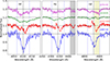 |
Fig. 1. Optical spectra from our database, zoomed in on the Balmer Hδ, Hγ, and Hβ transitions. They all show BAs with cores partially filled by the emission line. From bottom to top: J1807 (epoch 3 of dataset A, blue), J1727 (epoch 25, red), J1118 (epoch 1, green), and J1753 (epoch 2, magenta). Telluric bands and DIBs are shown as grey and yellow-shaded regions, respectively. The rest wavelength of the transition is marked with a dashed black line, while dotted blue lines mark velocity shifts of ±2500 km s−1 as a visual reference. |
2.1. Population database
We separate LMXBs according to the nature of their compact object (BH or NS) and compile their key physical properties.
2.1.1. Black holes
We base our sample on the BlackCAT catalogue from Corral-Santana et al. (2016). At the time of publication, the updated online version1 consists of 73 sources. We individually searched the literature for studies on each system that reported optical spectroscopy during an outburst episode. We searched for BAs in the available spectra, both through visual inspection of the plots and previous reports by the original authors. This analysis led to the following classification of the population (see Table 1):
Summary of the population study.
-
Uncharted (39): Optical spectra are not available for 39 systems, more than half of the known sample. The fact that most LMXBs are first discovered in the X-rays, together with their predominant presence across the Galactic plane, results in faint optical counterparts due to interstellar extinction (see e.g. GRS 1915+105, Av = 19.7, Chapuis & Corbel 2004). Limitations from the observing facilities at the time of the X-ray discovery (leading to shallower limiting magnitudes) or a slow follow-up response might also lead to the absence of optical spectroscopy. We also include in this class those systems for which optical spectroscopy was obtained, but their counterparts were later discarded as interloper stars in the line of sight (e.g., MAXI J1813 in Armas Padilla et al. 2019; MAXI J1631-479 in Kong 2019). Finally, we decided to add to this subsample 4U 1543−475, whose relatively early type companion dominates even during outburst (Sánchez-Sierras et al. 2023). Due to the broad and deep companion star stellar features, we cannot disentangle them from a potential BA, and therefore we cannot explore its presence.
-
BAs (17 confirmed + 2 candidates): A total of 19 systems exhibited BAs during at least one epoch of their outbursts (see Table A.1). Systems where BAs are observed in at least one other transition than Hβ (e.g., Hα, Hγ, Hδ) are referred to as confirmed BA sources (17). Due to the presence of a diffuse interstellar band (DIB) contaminating the red wing of Hβ, claiming the detection of BAs based on this sole line might be challenging. As a matter of fact, a blue-shifted absorption (such as those associated with outflows, see e.g. Mata Sánchez et al. 2023) combined with this DIB would mimic a BA-like profile. For this reason, we refer to the two systems where the BA report is based only on Hβ as candidates, namely GX339−4 and GRS 1716−249.
-
Non-BAs (5 confirmed + 10 candidates): The remaining 15 sources have published optical spectra during their outbursts, but no obvious BAs were neither reported nor identified through visual inspection. In this regard, we note that most systems have only one (for 7 BHs) or at most two (for 3 BHs) epochs of optical spectroscopy of sufficient signal to noise ratio (S/N) to detect the emission lines from the accretion disc. We refer to these ten sources as candidate non-BAs. The remaining five targets are GS 2000+251 (11 epochs; Borisov et al. 1989; Charles et al. 1991), V404 Cygni (59 epochs across different outbursts, Mata Sánchez et al. 2018), XTE J1550−564 (7 epochs reported but no figures available, Buxton et al. 1999), SAX J1819.3−2525 (V4641 Sgr, with at least 23 outburst epochs when the early companion does not dominate; Kiss & Meszaros 2004; Muñoz-Darias et al. 2018), and MAXI J0637−430 (four epochs during the same outburst, Strader et al. 2019; Tetarenko et al. 2021). Neither of them show BAs in spite of dedicated spectroscopic follow-ups, and they will be referred to as confirmed non-BAs. In spite of this classification, we remark that the non-detection of BAs on the available datasets does not forbid their presence at different epochs.
2.1.2. Neutron stars
The more prolific sample of LMXBs harbouring NSs allows us to expand our study independently of the compact object nature. We base our study on the most recent LMXBs catalogues published (Avakyan et al. 2023 and Fortin et al. 2024), from which we remove BH and BH candidates previously considered. As a result, our final sample of NS LMXBs consists of 285 sources, which we split among the following types using the same criteria defined in the previous section (see Table 1):
-
Uncharted (238): There is no optical spectroscopy available during outburst for the majority of our sample. Similar arguments to those drawn for BHs allow us to explain this situation. Additionally, 17 sources are within globular clusters, preventing the obtention of optical spectroscopy for the counterpart due to crowding. Furthermore, 6 LMXBs had optical spectra obtained during outburst, but their early type companion star’s contribution still dominated, preventing us from finding BA features.
-
BAs (7 confirmed + 2 candidates): A total of nine targets show BAs. We label MXB 1837+05 and Aql X-1 as candidates, given that the only transition showing a BA is Hβ. We also note that the subsample of confirmed BAs includes one ultracompact system (UW CrB), which has exhibited variable and broad absorption features (see e.g. Kennedy et al. 2025; Fijma et al. 2025).
-
Non-BAs (20 confirmed + 18 candidates): The remaining 38 systems correspond to those with published optical spectra during outburst, but without any trace of BA features. Candidates to non-BAs have either a single epoch (14 of them) or two epochs (4) of spectroscopy. On the remaining 20 targets, for which at least three epochs of spectroscopy were observed, BAs were not found in spite of the better coverage during the outburst event. Attending instead to the nature of the 38 non-BAs, we find 7 are candidates or confirmed transitional millisecond pulsars. These systems exhibit LMXB-like spectra during the so-called accretion powered state, but none has exhibited broad absorption features yet, maybe due to their low-luminosities compared to classic outbursting LMXBs. Furthermore, 11 systems are ultracompact candidates with hydrogen-poor companions, whose optical spectrum is either featureless or hydrogen-deficient (see e.g., Armas Padilla et al. 2023). Therefore, only 20 non-BAs correspond to traditional LMXBs, out of which 9 are confirmed and 11 are candidates.
2.1.3. Sample biases
We identify biases during the sample compilation that might have an impact on the results discussed in the following sections. First and foremost, we have access to spectroscopic data of a limited fraction from the (already small) known population: barely 34 BHs (47%) and 47 NSs (16%) have at least one epoch of spectroscopy. The scarce number of spectroscopic epochs obtained for most of the outburst events (only 23 BHs and 29 NSs have more than two epochs of observations) plays against the detection of these features, as they are not persistently observed (see Sect. 3). We are also biased towards the brightest systems in the optical range (whether due to their intrinsic brightness, their proximity to us or a lower extinction in their line of sight). Furthermore, our detection of BAs in the spectra depends on either literature reports or visual inspection of the published data. These features have traditionally not been the focus of their original studies, and as a result, we are naturally biased to mainly detect the deepest examples of BAs. Finally, BAs appear stronger at bluer wavelengths (see Sect. 3), but most optical studies have traditionally focused on the  range (covering He II−4686, Hβ, and Hα transitions). Together with the contaminant DIB on the red wing of Hβ, which forbids us from unequivocally confirming a BA detection if it is only present in this transition, it further reduces the number of detections. All of these biases affect our sample in the same way: the number of systems exhibiting BAs compiled in this work should be treated as a conservative lower limit of the true sample.
2.2. Spectroscopic database
In order to explore the evolution of BAs during outburst, dedicated spectroscopic datasets are required. To this aim, we construct a spectroscopic database which consists of six LMXBs where optical spectroscopy campaigns covered their outburst events and revealed BA features. This includes five BH transients either dynamically confirmed or established from Hα scaling relations (Swift J1727.8−1613, GRO J0422+32, XTE J1118+480, Swift J1753.5−0127, and Swift J1357.2−0933; which we refer to as J1727, J0422, J1118, J1753, and J1357, respectively), and one NS (MAXI J1807+132, hereafter J1807). A summary of the spectroscopic database is compiled in Table A.2.
The dataset for J1727 consists of 25 spectroscopic epochs (50 individual spectra) obtained with the 10.4-m Gran Telescopio Canarias (GTC) at the Roque de los Muchachos Observatory (La Palma, Spain), equipped with the Optical System for Imaging and low-Intermediate-Resolution Integrated Spectroscopy (OSIRIS, Cepa et al. 2000). The first 20 epochs were already reduced and published in Mata Sánchez et al. (2024), dedicated to the discovery outburst of the source. The remaining 5 epochs correspond to later observations obtained during the soft state decay and transition to a low-hard state (see Table A.2, also Sect. 4.3.1). We reduced them following the same prescription as in the original paper. We also flux-calibrated the spectra making use of spectrophotometric standard stars (Ross640, Feige 110, and GD191-B2B) observed at the end of the night for each epoch. This introduces uncertainties on the target flux calibration, as they were observed under different atmospheric conditions. We corrected for slit losses, considering wavelength dependent seeing and airmass correction. Once the spectra are calibrated in flux density units, we multiplied them by the transmission curves of the r- and g-band SDSS filters (Abazajian et al. 2009), and integrated the flux density over the wavelength dimension to obtain the optical brightness of the system on these photometric bands. J1727 data covered the full r-band regime in all 25 epochs with either the R1000B or R2500R grisms, while g-band was only fully covered with R1000B or R2000B in 20 epochs (excluding E5-E9).
We compiled two datasets for J1118. The first consists of 190 individual spectra distributed across 21 epochs during the outburst of 2000, previously published in Torres et al. (2002). Another 4 more epochs (167 spectra) covering a later outburst in 2005 are also included in this study. Three of these epochs were previously presented in Elebert et al. (2006), while the last of them remained unpublished to date. We obtained the reduced data for all epochs from the original authors, who followed the same prescription as in Torres et al. (2002).
A number of observations were reported for J0422 during its discovery outburst in 1992 and the following mini outburst a few months later. We identify three key datasets: Shrader et al. (1994), Casares et al. (1995a), and Callanan et al. (1995). Given that 30-year old spectra are not available in public repositories, we digitised the plots in the original publications to extract the spectra. We use WebPlotDigitizer2 (v5.2) to this aim. A total of eight spectra were obtained from Figure 5 in Shrader et al. (1994). They belong to the main 1992 outburst of the source and correspond to a period of seven months, covering a wavelength range of  . We also retrieved 10 spectra from Fig. 3 in Casares et al. (1995a). They correspond to the phase-binned average of 51 individual spectra obtained during four consecutive nights of the 1993 mini-outburst which followed the main event, covering
  . Finally, another eight epochs proceed from Fig. 5 in Callanan et al. (1995). They cover both the main outburst and the following echo outburst with different telescopes and instrumental setups. As a result, five spectra cover 4400 − 7000 Å, two include
  , and a single spectrum extends down to
  (see the original papers for further details).
We obtained four epochs of spectroscopy for J1753, a BH established from Hα scaling (Yanes-Rizo et al. 2025), during the initial epochs of its 2023 outburst. They were observed with the instrumental set up detailed in Table A.2, covering  . We reduced this data following the same standard process as for J1727. Observations of spectrophotometric standard stars allowed us to flux-calibrate this dataset and obtain simultaneous photometry in r and g bands, following the same description as for J1727.
We compiled a dataset of observations for the high-inclination BH J1357 (Mata Sánchez et al. 2015; Casares 2016) during its 2011 outburst event. It consists of a total of 4 epochs of spectra that were observed with different instrumental set-ups. The first epoch covers  , while the remaining spectra extend down to
  . Inspection of the individual spectra shows they remain stable within each epoch, so we focus our analysis on the averaged spectra for each epoch to increase the S/N. Data was provided and reduced by the authors of the original publications.
The spectroscopic dataset for J1807, the only NS of our sample, covers two outburst events. We analysed the data presented by Jiménez-Ibarra et al. (2019a), consisting of 6 epochs (covered by 9 individual spectra) obtained during the 2017 outburst. Details on the data reduction are in the original paper. In addition, we performed a spectroscopic campaign during the latest outburst of the source in 2023, consisting of 10 epochs (28 individual spectra) detailed in Table A.2. We reduced them following the same prescription as for J1727 datasets, which were obtained with the same telescope and instrument. Observations of spectrophotometric standard stars during J1807-B allowed us to flux-calibrate this dataset and obtain simultaneous photometry in r and g bands, following the same description as for J1727.
3. Analysis and results
3.1. Population analysis
We analyse physical properties of the LMXB population, split into BHs and NSs, which might impact on the formation and/or detection of BAs in their optical spectra. Among them, we focus on those readily available for most members of the sample, namely the orbital period (Porb), the distance to the source (d), and the height over the Galactic plane (|z|). For BHs, the orbital inclination (i) is also reported. Symbols and colours allow us to separate systems exhibiting BA features at any point of their outburst evolution from those that do not (non-BAs). The full sample is shown in Fig. 2, where the number of epochs (Nepochs) is plotted against the Galactic latitude (b). The remaining figures are limited to subsamples for which each pair of parameters is available. We have a systematically larger number of observed epochs among BHs than for NSs, as shown by a much larger fraction of uncharted targets for the latter (39/73, 53% for BHs; 238/285, 84% for NSs).
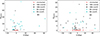 |
Fig. 2. b against Nepoch for the BH (left) and NS (right) population. Cyan symbols refer to systems with detected BA features (crosses for candidates, filled circles for confirmed systems), black symbols to non-BA systems (crosses for candidates, filled triangles for confirmed systems), and red dots to systems without available spectroscopic data (also known as uncharted). |
3.1.1. Orbital period
The distributions of Porb within the known BH and NS populations are shown in Fig. 3 (b against Porb). Visual inspection of this figure leads us to set a threshold at Porb ∼ 11 h for both BH and NS alike. For BHs, this choice splits the parameter space into short (22/33 sources) and long (11/33 sources) Porb. Non-BAs are evenly split, being half (5/10 sources) below the threshold. Most BA systems (83%, 15/18) are short Porb. Similar results are found for the NS population (Fig. 3, right panel), where 88% BAs (7/8), 66% non-BAs (20/30), and 68% of the full NS population (100/146) lie below the threshold. Similar disc sizes in NSs and BHs require a longer Porb (by a factor of ∼2 − 3) for the former, due to the lighter compact object mass. This might justify pushing the threshold for NSs to longer values, effectively removing the only BA candidate above the threshold. We decided to keep the same threshold for both populations in order to discuss a more conservative scenario. We explored the non-BA and BA period distributions to assess whether they belong to independent populations (analysing BHs and NSs separately). An Alexander-Govern test (A = 1.46 and p = 0.23 for BHs; A = 1.04 and p = 0.31 for NSs) did not allow us to reject the null hypothesis in either case.
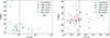 |
Fig. 3. Porb against b for the BH (left) and NS (right) population. The colour and symbol description matches that of Fig. 2. The dashed black line marks the 11 h threshold described in the text. |
Given our limited sample size, we are able to individually inspect the few BA outliers with Porb above the threshold. Among NSs, the sole exception is Aquila X-1 (Porb = 18.95 h, Garcia et al. 1999), a candidate BA where only Hβ exhibited this feature at certain epochs (Panizo-Espinar et al. 2021). The remaining 10 sources above the period threshold for which optical spectra have been obtained are all non-BAs (most of them confirmed). Among the BH population, there are three long-period systems which exhibit BA features: a candidate BA (GX339−4; Porb = 42.21 h, Heida et al. 2017) as well as two confirmed BAs, namely GRO J1655−40 (Porb = 62.92 h, Soria et al. 2000) and MAXI J1820+070 (Porb = 16.45 h, Torres et al. 2019). The latter has been extensively observed (86 epochs over two different outbursts; see e.g., Muñoz-Darias et al. 2019 and Sai et al. 2021), but BAs have only been found in two epochs (Garnavich & Littlefield 2018; Yoshitake et al. 2024). On the other hand, the detection of BAs in GRO J1655−40 is much more frequent (Soria et al. 2000). These observations suggest that, while BAs are not typically observed in long Porb, its detection is not forbidden.
At this point, it is worth remarking that the larger accretion discs associated to a long Porb can sustain longer outbursts. Given the transient detection of BAs, a more exhaustive coverage of the outburst might be required to properly cover the whole event, which could introduce an observational bias against their detection. However, we note that no BAs are found in systems with intensive coverage of their outburst (see in particular V404 Cygni, Mata Sánchez et al. 2018 and SAX J1819.3-2525, Muñoz-Darias et al. 2018). Together with the absence of definitive BA confirmation in any NS above the threshold, we conclude that BAs are preferentially shown in short Porb systems.
3.1.2. Orbital inclination
Arguably the most elusive parameter to measure in LMXBs is i. As a result, we have measurements for a limited number of systems. There are 25 BHs for which i has been measured or constrained, with uncertainties varying greatly from system to system. We collected them from the BlackCAT catalogue (Corral-Santana et al. 2016), updated with the best i measurements reported in Casares et al. (2022), and added the low inclination system MAXI J1836−194 (i = 4 − 15 deg) as measured in Russell et al. (2014). To analyse the dependence with i, we define three different ranges: low inclination (≲30°), medium inclination (30 − 60°), and high inclination (≳60°). Plotting these separate ranges (see Fig. 4) allows us to determine that 11% of the BHs are low-inclination, 31% are mid-range, and 58% are high inclination. This distribution is consistent with randomly oriented orbits (i.e. uniform in cosi, favouring edge-on inclinations), which predicts 13.5%, 37.5%, and 50% for the low, mid, and high inclination ranges, respectively. This suggests a homogeneous sampling in spite of the limited number of systems. No clear connection between this physical parameter and the detection of BA features is observed. We nevertheless acknowledge that our sample is limited, specially among low inclination systems, precluding a detailed inspection. Indeed, low inclination LMXBs are intrinsically harder to characterise, due to both the uniform distribution in cosi and their weak ellipsoidal modulation in quiescence (from which most determinations of i are obtained).
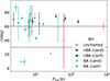 |
Fig. 4. Porb against i for the BH population. The colour and symbol description matches that of Fig. 2. Dashed lines mark the thresholds at 30° and 60° that define the low, mid, and high inclination regions. If only constraints to the i parameter are available, we plot the central value and use the range as the associated uncertainty. |
3.2. Outburst-resolved spectroscopic analysis
In order to explore the evolution of BAs during outburst, we performed a dedicated study on six LMXBs where optical spectroscopy campaigns covered their outburst events and revealed BA features (see Sect. 2.2). We analysed the Balmer series (Hα, Hβ, Hγ, and Hδ transitions), with a particular focus on bluer transitions as they have exhibited the most prolific examples of BAs. To systematically assess the properties of BAs, we normalise each transition independently through the fit of a low order polynomial to the nearby continuum of each of the lines of interest, for each individual spectrum. The typical profiles of the Balmer series follow that of a canonical accretion disc (broad, double-peaked emission lines) embedded into a BA. To systemically capture the BA properties, we designed the following toy model.
The emission component is fitted with a double Gaussian profile. The height of both Gaussians is controlled by the area of the red peak (Ared) and the intensity ratio between the blue and red peaks (Iratio = Ablue/Ared), to allow for asymmetric profiles. For consistency, we define the area of the full double peak profile as |EWemi|=Aredi ⋅ (1 + Iratio). Given that we are working with normalised spectra, this parameter is effectively the equivalent width (EW) of the emission component, where we follow the convention of positive values for absorption features and negative for emission features. The profile centroid is controlled by the offset (μ) parameter (referred to the rest wavelength of each transition), the separation between the Gaussians’ centroids is DP and the width of each Gaussian is defined through σ. Other than |EWemi|, which determines the area of the individual transitions, the remaining parameters are linked for all simultaneously fitted lines in each individual spectrum.
We tested three different profiles for the absorption component: Gaussian, Lorentzian, and a Voigt function. Our tests showed that, while all three resulted in reasonable fits, the best-fitting χ2 for the Gaussian profile was slightly but systematically better than its Lorentzian counterpart, and that the Voigt profile fit always preferred a null contribution for the Lorentzian component. For this reason, we hereafter report only the results from a Gaussian fit to the absorption component, controlled by a common centroid (μabs), as well as independent width (σabsi) and depth (defined by the area of the absorption component, EWabsi) for each transition. Both σ and σabsi parameters were corrected from the corresponding instrumental resolution on each measurement. To obtain the best fit to each spectrum we employ a python script based on EMCEE, an implementation of a Markov Chain Monte Carlo (MCMC) sampler (Foreman-Mackey et al. 2013). We define the likelihood function as the χ2 resulting from the comparison to our model, and report 16, 50, and 84% quantiles of the marginalised distributions for each fitted parameter (corresponding to 1σ uncertainties for a Gaussian-like distribution) in Table B.1. It follows a dedicated study for each target.
3.2.1. Swift J1727.8−1613
The J1727 spectroscopic sample was partly introduced (E1–E20) in Mata Sánchez et al. (2024), where the authors mention the development of BAs in the Balmer series as the outburst evolves. The extended dataset we present in this work includes 5 further epochs (E21–E25) where BAs become more prominent. We fitted all epochs with the model previously defined (see Fig. C.1). Both the nearby DIB ( ) and the He I-
 emission line appear close to the Hβ line, and they could bias the results from our fit. For this reason, we decided to mask out the affected region at the red wing of Hβ, even though this diminishes our detection sensitivity to potential BAs on this line. The resulting best-fitting parameters are shown in Fig. C.2. The overall description of the fitting results follows. We focus exclusively on those fits resulting in a detection of BAs over the 3σ limit for the EWabs parameter in at least one of the transitions.
The behaviour of the emission component parameters is typical from accretion discs in LMXBs. The double peak profile does not become particularly asymmetric, and the width of the Gaussians is remarkably stable over the whole outburst. We identify two regimes where the behaviour of DP changes significantly (by a factor of ∼2, see Table B.1). We refer to them as the narrow-line regime (E1–E20), corresponding to the hard, hard-intermediate (HIMS), soft-intermediate (SIMS), and initial soft state decay; and the broad-line regime (E21–E25), limited to the low-luminosity soft state and the transition to the low-hard state. The regime swap occurred between two epochs separated by a 4-month gap (due to Sun constraints) during the soft state X-ray decay. |EWem| evolves smoothly, being systematically weaker for shorter wavelengths across the full sample. The centroid of the emission ( ) is consistent with the systemic velocity (γ = −181 ± 4 km s−1; Mata Sánchez et al. 2025), supporting its association with the accretion disc of the binary. We nevertheless note its large standard deviation, which reveals significant variability on the parameter during the outburst, specially during the narrow-line regime.
During the narrow-line regime, the absorption component remains either undetected (as for the majority of Hβ and Hγ, considering a 3σ threshold) or shallow (Hδ,  ). The broad-line regime shows a smooth increase in the parameter for all transitions, reaching a maximum of
  for Hδ. The width of the absorption is consistently broad for the Hδ transition across both regimes (
 ). On the other hand, Hγ and Hβ absorptions are narrow and variable during the initial regime but they become broad and consistent with Hδ after the transition to the broad-line regime. Finally, we note the centroid of the absorption shows large variability (similar to the emission component), still consistent with the systemic velocity.
Given our intensive coverage during the outburst event, we also analysed a potential dependency of the measured parameters with the orbital phase. To this aim, we employed the ephemerides from Mata Sánchez et al. (2025). We found no orbital dependency for any of the parameters, suggesting the profile changes are rather linked to the outburst evolution.
3.2.2. XTE J1118+480
We have over 350 spectra from two outbursts of J1118, namely the 2000 and 2005 events. We first inspected the spectral evolution within each epoch. The most prolific example is E22, with 59 consecutive spectra covering over 5 h. We find that the best fitting parameters remain stable during the whole dataset. This result holds for each of the epochs analysed, proving the stability of BAs features over periods of at least a few hours. Hereafter, we focus on the averaged spectrum for each epoch. We have access to 21 epochs covering the 2000 outburst and four further epochs during 2005. Both outburst events were hard-only outbursts, with low X-ray luminosity (see Zurita et al. 2006). The 2000 outburst was covered during four consecutive months, while the outburst remained stable in X-rays (∼1.5 − 2.5 counts s−1 flux variability, see Torres et al. 2002). The 2005 outburst coverage is scarcer, but includes the outburst peak and decay (R ∼ 13.5 to R ∼ 14.5 during E21–24, and dropping to R ∼ 16.5 on E25, see Zurita et al. 2006). We fitted the spectra following the general prescription (see Figs. C.3 and C.4). We find no clear differences between the 2000 and 2005 outbursts in any of the fitted parameters, so we analyse the dataset as a whole.
The emission component centroid velocity μem is highly variable, with a mean and standard deviation of  (consistent with the systemic velocity of 16 ± 6 km s−1; Torres et al. 2004). The peak-to-peak ratio is similarly variable, with epochs of particularly asymmetric profiles (e.g., E9). The emission component width and double peak separation are stable across both outbursts. The |EWem| evolves smoothly and remains below
  during the entire dataset.
The absorption component is consistently broad over the whole outburst event, particularly for Hδ ( ). EWabs follows a similar behaviour, where Hδ exhibits the deepest BA examples, peaking at E25 with
  , corresponding to the faintest epoch recorded. The centroid of the absorption component is remarkably variable as well. We performed a Lomb-Scargle periodogram on μabs and found maximum power at a period of ∼53 d for the 2000 outburst event, consistent with the disc precession period (see Sect. 4.3.3). A sinusoidal fit to our limited dataset resulted in a radial velocity semi-amplitude of ∼240 ± 30 km s−1, oscillating around a central velocity of ∼260 ± 30 km s−1, notably offset from the systemic velocity.
3.2.3. GRO J0422+32
The sample for J0422 has limited and uneven spectral coverage. It did not exhibit the X-ray characteristic features indicating a transition to the soft state, neither during the main outburst in 1992, nor during the subsequent minioutburst in 1993 (see e.g., Shrader et al. 1997). For this reason, we consider them all as hard-only outbursts (see e.g., Alabarta et al. 2021). We analysed the three datasets separately (A, B, and C; see Table A.2). The systemic velocity is 11 ± 8 km s−1 (Harlaftis et al. 1999).
Dataset A shows eight spectra obtained from August 1992 to March 1993, covering the main 1992 outburst with a monthly cadence. They cover Hδ to Hβ. The emission component shows highly variable radial velocity and Iratio, while stable σem and DP (after removing an outlier in A4). The absorption component seems consistently blue-shifted during most of the outburst A1–A7 ( ), but redshifted by the end of it (A8,
  ). The width and depth of the BA are variable, but overall consistent across the explored transitions, showing deeper profiles in bluer wavelengths.
Dataset B spectra consistently covers Hγ and Hβ. It corresponds to a phase-folded set of spectra obtained during the initial decline of the 1993 December mini-outburst. The short period when these observations were obtained (four consecutive nights) allows us to inspect the evolution of the BAs on short timescales. Most of the emission and absorption component parameters are stable at typical values (except for an outlier on epoch B3). The original paper (Casares et al. 1995a) reported that the emission component of Balmer lines experienced Doppler-shifting at the orbital period of the system with semi-amplitudes of the order of  . We confirm this trend for the emission component in Hγ and Hβ, varying around a mean velocity of
  , consistent with the systemic velocity. A similar analysis reveals periodic variability for the absorption component centroid μabs. We performed a sinusoidal fit to this parameter and obtained a radial velocity semi-amplitude of ∼48 ± 10 km s−1, slightly off-phase compared to the known ephemerides (ϕ0 = 0.10 ± 0.03) and oscillating around a central velocity of ∼146 ± 7 km s−1, significantly larger than the systemic velocity.
For dataset C, the uneven spectral coverage led us to mainly focus on Hβ for the analysis, and include Hγ when present. The observations span over a year, including a short period at the beginning of the 1992 outburst (C1–5) as well as the 1993 mini outburst (C6–8). The 1992 outburst starts by exhibiting relatively deep BAs in Hβ (up to  in C1), becoming shallower as the outburst evolves (
 in C5). During 1993 outburst, the BAs are less variable, and exhibit values comparable to those of the final epochs of 1992 outburst. The width of Hβ BAs remains stable across all epochs. The centroid velocity is highly variable during 1992 outburst, from ∼ − 500 km s−1 in epoch C1 to ∼50 km s−1 in epoch C5. During the 1993 minioutburst, the radial velocity is stable and consistent with C5.
3.2.4. Swift J1753.5−0127
Observations were performed during the outburst of the source that started on September 28th 2023 and lasted ∼5 months (Alabarta et al. 2024) We obtained four epochs that allow us to explore the Hβ, Hγ, and Hδ transitions. These epochs were obtained during the initial rise of the 2023 outburst (days 5–15, referred to the outburst trigger on HJD 2460215.5), and before the source reached a plateau in optical brightness (r ∼ 17, Alabarta et al. 2024). The few references regarding X-ray observations at the time of publication suggest the source was in the hard state during our four epochs (Alabarta et al. 2023). We focus on the Balmer series to compare with the rest of the population, but we note that a BA appeared on He II–4686 (E1, see Sect. 4.5).
The emission component is stable over the duration of our observations (Fig. C.5), with typical values comparable to the rest of the sample and a centroid velocity consistent with the systemic value (131 ± 55 km s−1, Yanes-Rizo et al. 2025). The centroid velocity of the absorption component is also consistent with the above. However, contrary to other systems where the BAs become deeper at later epochs of the outburst, J1753 exhibits the deepest example on the initial observation ( on Hδ during E1). In this regard, it is worth remarking that our initial epoch is the faintest of our sample, obtained during the outburst rise. Table B.1 compiles the mean values for each fitted parameter, but given the low number of spectra (only E3 and E4 show > 3σ BA detections), individual measurements dominate.
3.2.5. Swift J1357.2−0933
The limited wavelength coverage of the four epochs observed for J1357 only makes Hα and Hβ available for our study. We fitted the averaged spectra corresponding to four epochs (days 27, 47, 72, and 101 referred to the outburst trigger). The outburst peaked soon after its discovery, and remained in the hard state as the luminosity decayed. BAs clearly developed in the later, lower-luminosity epochs (see Fig. C.6). A systemic velocity of γ = −130 ± 17 km s−1 was proposed by Jiménez-Ibarra et al. (2019b) based on the emission line analysis in outburst, as the companion star features remain undetected even in quiescence (see e.g., Torres et al. 2015; Mata Sánchez et al. 2015; Anitra et al. 2023).
We fit the line profiles and reported the averaged values in Table B.1, though the scarce number of spectra makes them dominated by individual measurements. The emission component is similar to that observed in other members of our sample, being the most remarkable feature its large DP = 1707 ± 13 km s−1, consistent with its optically dipping nature. BAs show quite variable centroids, with a minimum of  (E3) and a maximum of
  (E4). The maximum depth of
  is observed for Hβ on E4, being also the broadest BA of our sample (
 ).
).
3.2.6. MAXI J1807+132
The dataset for J1807 covers the 2017 (6 epochs) and 2023 (10 epochs) outbursts. Jiménez-Ibarra et al. (2019a) proposed a systemic velocity of γ = −145 ± 13 km s−1, based on a line fitting model (similar to that employed in our study) to dataset A spectra, but including a larger set of lines (e.g. Hα, He II–4686).
Only three spectra from the 2017 dataset have enough S/N to perform meaningful fits (A1–3, Jiménez-Ibarra et al. 2019a). They correspond to a short period spanning two weeks. Comparison of the photoindex observed in Jiménez-Ibarra et al. (2019a) with the later 2023 outburst (Rout et al. 2025) suggests the system was in the hard state during 2017 observations. The best fitting model reveals consistent parameters for the emission component, including a centroid velocity matching the systemic velocity. Regarding the absorption component, σabs is quite stable, while EWabs increases from A1 to A3, reaching a maximum in Hδ of  . The centroid of the absorption retains positive velocities, again consistent with the systemic velocity.
During its 2023 outburst, J1807 exhibited the canonical X-ray behaviour of an LMXB (Rout et al. 2025). The ten epochs we observed are associated with their corresponding X-ray state following the aforementioned paper (see Figs. C.7 and C.8). Both the emission and absorption components followed the same behaviour as observed in 2017, with a maximum  being achieved by Hδ during B6. J1807 study shows how similar BAs resurge from the same source in two different outburst episodes six years apart, developing across all X-ray states.
3.2.7. Combined analysis of the spectroscopic sample
We searched for correlations between the fitted parameters in the combined spectroscopic database. To this aim, we analysed all possible pair combinations, employing the Spearman’s correlation coefficient (rs) to assess their strength. The strongest correlation (the only above rs ∼ 0.7) is found for EWabs, Hβ against EWabs, Hγ (Fig. 5, right panel; rs = 0.89). A linear fit to the full sample reveals a line ratio of EWabs, Hβ/EWabs, Hγ = 1.05 ± 0.05. To further investigate this, we also analysed the weaker correlation (rs = 0.63) between EWabs, Hγ and EWabs, Hδ. A linear fit reveals EWabs, Hγ/EWabs, Hδ = 0.67 ± 0.05, suggesting that Hδ is systematically deeper than redder transitions. Flux ratios of absorption lines trace the physical conditions of the line forming region, being particularly sensitive to density and temperature. The inspected transitions cover a narrow range of wavelengths ( ), so under the assumption of a flat continuum contribution at this range, EW ratios might be a proxy for the flux ratios. Although we do not have access to enough transitions to extract reliable physical parameters (see e.g. Ilić et al. 2012), the stability of the line ratios suggests physical conditions of the BA forming region remain stable. This occurs both during the outburst evolution and for all systems analysed, in spite of the extreme variability of the optical continuum, supporting a scenario where BAs are persistent.
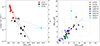 |
Fig. 5. Left panel: EWabs, Hδ against r-band brightness (left axis for flux density units, fν; right axis for absolute magnitudes, Mr) from the best-fitting results of the subsample with flux-calibrated spectra. The colour code marks the systems associated with each data point. A dashed black line depicts the best linear fit to the correlation, and dashed cyan, dashed red, and dashed black lines are the equivalent for individual datasets. Right panel: EWabs, Hβ against EWabs, Hγ from the best-fitting results of the whole spectroscopic sample. The colour code marks the systems associated with each data point, while symbols differentiate between subsets as described in the legend. A dashed black line depicts the best linear fit to the correlation, which is consistent with a 1:1 ratio. Transparent symbols correspond to fitting parameters that are consistent with null BA within 3σ. |
We also produced histograms combining fits to all members of the sample, focusing on parameters describing the BA. We study the joint results for the Hβ and Hγ line profiles, consistent with each other (see Fig. 6). Hδ was not included in the histogram because it suffers from systematically lower S/N and overall scarcer sampling. We find that the distribution of centroid velocities (corrected from their respective systemic velocity) has a mean and standard deviation of  . The spread is large, but it remains fully consistent with that of the emission component (μ = 100 ± 180 km s−1). This shows that the BAs in our sample are not systematically blue-shifted. The width of the BA σabs is quite stable, showing a Gaussian distribution with mean and standard deviation of
  . Finally, the typical depth of the features are
  . In this regard, we note that the deepest examples occur at low luminosities, reaching
  (and even deeper in Hδ,
  in J1753).
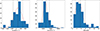 |
Fig. 6. Histograms of the spectroscopic database for μabs, σabs, and EWabs (combining the results for Hβ and Hγ, which produced consistent distributions). The continuous and dashed black lines mark the mean and 1σ of the distribution, respectively. A Gaussian fit to the histogram is also shown as a red line. |
Certainly, the observation of deeper BAs at fainter epochs appears a general property of our sample (see e.g., E25 in J1118). To test this, we compare the fitted parameters of the spectroscopic sample against the brightness of the source at the time of observations. We only have simultaneous optical photometry for J1727, J1807-B, and J1753 datasets (see Sect. 2.2). In order to compare all systems, we decided to convert their apparent magnitudes to absolute magnitudes. To this aim, we employed the best-fit extinction and distance reported for each source, namely: d = 3.4 ± 0.3 kpc, E(B − V)=0.6 ± 0.3 for J1727 (Mata Sánchez et al. 2025); d = 6.3 ± 0.7 kpc, E(B − V)=0.099 ± 0.008 for J1807 (Saavedra et al. 2025); and d = 3.9 ± 0.7 kpc, E(B − V)=0.45 ± 0.09 for J1753 (Yanes-Rizo et al. 2025). The resulting absolute magnitudes were plotted against all the available parameters from the spectral line profile fits. We find an inverse correlation (rs = 0.9) between the brightness of the system and the EWabs, Hδ (see Fig. 5, left panel). A linear fit to this correlation results in Mr = (1.1 ± 0.5)+(0.70 ± 0.11)EWabs, Hδ (and similarly, Mg = (1.0 ± 0.7)+(0.75 ± 0.15)EWabs, Hδ). There is a clear outlier to the linear correlation, corresponding to the deepest BA observed in J1753 sample. We nevertheless note this was obtained at the faintest epoch during the rise of the outburst, and that it remains consistent within 3σ (due to the larger uncertainties). The fact that the datasets of three different systems (two BHs and a NS) follow a common correlation implies that the compact object nature is not key to develop BAs. Furthermore, it shows that the optical luminosity range where BAs are visible is quite extended, spanning eight magnitudes.
4. Discussion
The above analysis revealed a number of common features for BAs, which allows us to systematically study these features for the first time. From the population analysis, we find the following key characteristics:
-
Ubiquity: They have been observed in 78% of BHs with at least three epochs of optical spectroscopy, as well as in 29% of NSs; a firm lower limit due to BAs transient visibility.
-
Frequent at short periods: They are more frequently observed below
 for both BH and NS systems alike.
 -
Non-dependent of i or compact object nature: BAs occur at all orbital inclinations, as well as for BHs and NSs alike.
-
Only seen in outburst: No BA features have been reported in the quiescent state of neither CVs nor LMXBs.
-
Predominantly shown in the H Balmer series: Its presence in other atomic species is limited to a handful of examples. These reports mainly refer to the He II−4686 line; in particular, GRO J0422+32 (originally reported in Shrader et al. 1992, but not mentioned/shown in Shrader et al. 1994); Swift J1753.5−0127 (observed in E1, during the initial rise of 2023 outburst); and Swift J1357.2−0933 (appearing only during the optical dips, Jiménez-Ibarra et al. 2019b). Even fewer examples exist for He I transitions: 3A 0620 shows a BA in He I−4471; Ciatti et al. (1977).
The study of our spectroscopic database reveals:
-
Deeper features at shorter wavelengths: If Hδ transition is available with sufficient S/N, it systematically exhibits deeper examples of BAs.
-
Slow profile evolution: Hydrogen Balmer emission lines from the accretion disc or the disc wind have been seen to evolve drastically during outburst, within timescales as short as just a few minutes (see e.g., Mata Sánchez et al. 2018, V404 Cygni). On the other hand, BAs evolve at a slower pace, and once they appear, they are sustained over long periods (e.g., AT2019wey shows deep broad absorptions in the Balmer series through several months; Yao et al. 2021). The only example with fast cadence observations of our database (J1118) showed stability over periods of at least a few hours.
-
They are deeper in fainter epochs, and otherwise independent of the X-ray state: There is an inverse correlation between EWabs and optical brightness, common among different systems and outburst epochs. BAs are equally observed in the hard and soft states.
-
Their centroid velocities are variable but their mean is consistent with the systemic velocity: They oscillate around the central value, without preference towards red-shifted or blue-shifted velocities and detached from the emission component.
-
Their width is stable: They follow a Gaussian distribution both during outburst and across systems (
 ).
). -
The normalised Balmer line ratios for the BAs remain constant: This suggests similar conditions of temperature and density at the BA forming region, independently of the system and/or outburst state.
4.1. Precedents of BAs in CVs
Cataclysmic variables (see Warner 1995 for general review) are a natural benchmark to test accreting compact systems phenomenology due to their more prolific population (over 104, see e.g. Jackim et al. 2020). There are reports of BAs in their spectra during active outburst phases since the onset of the field (Joy 1940). They have been found in both persistent (i.e. nova-like, disc-dominated; e.g. UX UMa; Neustroev et al. 2011) and transient (i.e. dwarf novae; e.g., GW Lib, SS Cyg and V455 Andromedae; see van Spaandonk et al. 2010; Hessman et al. 1984, and Tovmassian et al. 2022, respectively) CVs. Studies report BAs in H and He I with very broad full-width at zero intensity (FWZI  ), and cores filled by a narrower emission component (e.g., Szkody et al. 1990). BAs in CVs are comparable to those compiled in this work for LMXBs (see e.g., Hβ in Figs. C.1 and C.7, with wings reaching the mark of
  , i.e. FWZI
  ). Morales-Rueda & Marsh (2002) report on 40 systems where BAs are observed, whose Hγ BA properties are consistent with (though slightly narrower than) our LMXB sample.
Models considering the absorption originates from an optically thick accretion disc were developed to explain these features (e.g. Herter et al. 1979; Cheng & Lin 1989). Despite their limited success reproducing observational profiles, they all agree that BAs should be more prominent in low i systems due to limb darkening. Herter et al. (1979) model considers the broadening of the line is, for i > 15 deg, dominated by Doppler broadening. However, they expected a flat-bottom core for such a broadening profile, which is not observed. Instead, Gaussian-like profiles are found (as we do for LMXBs), which led them to suggest pressure broadening must be at play as well. As a result, they state BAs are formed in a region of the disc somewhat denser than the line-forming regions. When the outburst triggers, the disc begins to transition from an optically thin (quiescence) state to an optically thick state. As the instability wave propagates, ionizing the gas, the former emission lines gradually develop an absorption component, leading to mixed profiles. There are several reports of BAs becoming deeper as the CV brightens during the outburst and the core emission diminishes (see Hessman et al. 1984; Szkody et al. 1990; Clarke et al. 1984; Tovmassian et al. 2022 and references therein). Their EW increases during the outburst rise, only to remain stable during the rest of the event until they vanish during the decay to quiescence (e.g. Clarke et al. 1984). These studies claim that BAs might always be present, and their visibility would be conditioned by the filling of the emission core component.
4.2. The current BA view on LMXBs
In spite of the frequent appearance of BAs in LMXB spectra, they have been systematically set aside, as they hampered the study of other phenomena of interest. Among the few works mentioning BAs, Dubus et al. (2001) discussed them in a paper dedicated to J1118 outburst. They briefly compared their findings with previous detections in a handful of systems from the literature, as well as described a qualitative and phenomenological picture inspired by previous CV studies (e.g., Sakhibullin et al. 1998). According to this scenario, emission lines (which usually dominate LMXB outburst spectra) are produced in an optically thin (cromosphere-like) region above the accretion disc as a result of photoionisation by soft X-rays. On the contrary, BAs are formed in a lower, optically thick region of the accretion disc, where the temperature stratification with height over the orbital plane resembles that of a stellar atmosphere (see Fig. 7). Following this picture, a number of predictions were stated:
-
(i)
The formation of BAs depends on the spectral energy distribution of the irradiating X-ray flux. Soft X-rays are responsible for heating up the optically thin region responsible for the emission lines. On the other hand, hard X-rays penetrate deeper into the accretion disc, enhancing the temperature at the base of the optically thick atmosphere. For this reason, harder X-ray spectra might favour the formation of BAs.
-
(ii)
High values of overall X-ray luminosity might lead to the photoionisation of deeper layers, ultimately reaching the region of the accretion disc producing the BAs, and inverting the profile temperature. Therefore, BAs might disappear at high luminosities. If the optically thin atmospheres in LMXBs are more extended than those observed in CVs (an expected feature due to the larger irradiation), BAs should be less frequently observed in LMXBs than in CVs.
-
(iii)
Limb-darkening has a larger impact on systems with edge-on orbital inclination, as photons do not penetrate as deep into the accretion disc atmosphere as in a face-on case configuration. As a result, the formation of BAs should be inclination dependent, being shallower for edge-on systems.
The authors analysed these predictions on a handful of systems compiled from existing literature, which supported their conclusions. However, our work involving the whole BH population shows otherwise, as described in the following sections.
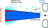 |
Fig. 7. Schematic of the model for BA formation. The white cloud on top of the compact object is the illuminating X-ray source (e.g. the base of the jet or the corona). It emits both soft (cyan) and hard (black) X-ray photons. The former heats up the disc chromospheric region and gives rise to emission lines, while the later contributes to heating up deeper layers of the accretion disc. This produces a stellar-like temperature profile, with a relatively cold region on the surface producing the observed BAs. Note that the accretion disc also exhibits a radial gradient of temperature, so only the outermost rings develop such a region. |
4.3. Testing the model predictions
4.3.1. Brightness and X-ray hardness
Broad absorptions have never been detected in quiescence, even for systems that exhibit them during outburst. The optically thin, low-viscosity accretion discs found in quiescence favour the formation of emission lines. Combined with veiling effects (as the relative companion star contribution increases) and the broader emission line wings (as the accretion disc contracts), the non-detection of BAs in quiescence is expected. During outburst, an optically thick photosphere develops as a result of internal viscous heating, enabling the formation of absorption profiles. Following Dubus et al. (2001) model described in the previous section, the BA formation would then depend on both the overall luminosity of the system and its X-ray spectral state.
Our spectroscopic analysis shows that BAs become deeper at fainter epochs (see Fig. 5, left panel). This is the opposite behaviour to that reported for CVs (see Sect. 4.1), which develop deeper BAs as their luminosity increases (see e.g. Hessman et al. 1984). The brightest CVs (∼1029 − 33 erg s−1) are comparable to the faintest LMXBs (∼1033 − 36 erg s−1; see e.g., Armas Padilla et al. 2013), especially if we rescale them by their Eddington luminosity. This might suggest that the luminosity dependence of the BA formation mechanism saturates at this intersection (∼33 erg s−1). CVs continuum during outburst is dominated by internal viscous heating of the accretion disc. Therefore, brighter CVs overall correspond to hotter and deeper layers of the accretion disc, favouring the formation of stronger BAs. On the contrary, the continuum in LMXBs is dominated by soft X-ray reprocessing of the central source irradiation at the accretion disc atmosphere. As such, brighter LMXBs do not necessarily translate into heating at the base of the accretion disc. At high luminosities, the disc atmosphere expands due to Compton heating from the X-ray irradiation, making the observability of BAs a balance between the relative depth of the absorption and emission components. As a result, BAs become weaker in bright LMXBs due to being (i) filled by a stronger emission component; and (ii) veiled by the extremely variable X-ray reprocessed continuum (given that EW is a normalised measure relative to the continuum).
Regarding the X-ray state dependence, our analysis shows BAs are detected during both hard and soft states alike for the two systems exhibiting full transitions (J1727 and J1807). In particular, J1727 (see Fig. 8) allows us to study the BA evolution over a full outburst event, showing that it is mainly driven by the continuum brightness rather than being linked to X-ray state transitions. The remaining systems exhibit hard-only outbursts, which prevented us from performing a more detailed study.
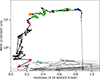 |
Fig. 8. Hardness-intensity diagram of J1727 (arrow-connected black dots; grey for low X-ray fluxes with colours possibly affected by background subtraction). The coloured symbols mark the epochs where our optical spectroscopy was obtained. The filled circles mark spectra where no BAs were detected, while filled stars correspond to BA detection in at least one of the inspected transitions (see Section 3). The colour code separates the initial rise in the hard state (blue), hard-intermediate state (HIMS, green), and soft-intermediate state (SIMS, orange), as well as the soft state decay (red). The last five epochs, published for the first time in this work, correspond to the final decay during the soft state and the subsequent transition to the low-luminosity hard state (cyan). |
We therefore conclude that BAs are present and remarkably stable over a wide range of luminosities, and only truly vanish when they return to quiescence.
4.3.2. Orbital inclination
The population analysis already showed that the distribution of i for LMXBs with BAs is perfectly consistent with randomly oriented orbits (see Sect. 3.1). There are no hints of shallower BAs for edge-on systems, contrary to the model prediction. Our spectroscopic sample allows for a closer inspection: J0422 is in the low-intermediate region (∼10 − 50 deg, Casares et al. 1995b; Beekman et al. 1997; Webb et al. 2000), J1727 inclination is only loosely constrained by an upper limit of 74 deg (Wood et al. 2024; Mata Sánchez et al. 2025), and the remaining targets are in the high inclination regime: J1118 (68 − 79 deg, Khargharia et al. 2013), J1807 (i = 72 ± 5 deg, see Saavedra et al. 2025), J1753 (79 ± 5 deg, Yanes-Rizo et al. 2025), and the most edge-on system known J1357 ( , Casares et al. 2022; see also Corral-Santana et al. 2013; Mata Sánchez et al. 2015).
The largest EWabs is found for J1753 in the Hδ transition, one of the most edge-on systems of our BH sample. The following systems in terms of EWabs are J1357, J1118, and J1807 (again at the higher end of i), which shows consistently large values at all inspected transitions. The lowest EWabs is found for J1727, for which we only have an upper limit to the inclination suggesting a mid-range value at most. Finally, the most face-on system of our sample (J0422) shows EWabs measurements between those of J1807 and J1727. In this regard, we note that J0422 inclination has been recently proposed to be as high as i = 56 ± 4 deg (Casares et al. 2022). This opens the possibility of J1727 being closer to face-on than the former. We also explored the width of the BAs (σabs, see Fig. 6), and found that only J1727 ( ) is consistently below the typical values of our sample (σabs = 1400 ± 500 km s−1, which updates to
  if J1727 is removed). In order to further explore the inclination dependence, we turned to the most extreme example for a low-inclination system among the full BH population exhibiting BAs: MAXI J1836−194 (4 − 15 deg, Russell et al. 2014). The authors performed a Gaussian fit to the absorption component and found
  and
and  for Hβ and Hγ, respectively, as well as
  and
and  . Compared with the sample presented in our work, the features in MAXI J1836−194 are on the lower end of our spectroscopic sample (see Fig. 6).
We conclude that lower i does not produce stronger BAs, contrary to the model prediction. Instead, based on the few available examples of low-inclination LMXBs, their BAs actually appear narrower, which further supports the existence of a Doppler broadening mechanism for BAs.
4.3.3. Orbital period and the system size
The orbital period is a proxy for the size of the system, and in particular to that of the accretion disc (given the late type companions and low mass ratio of LMXBs with BHs). A similar statement holds for NSs, even though they have smaller discs than BHs for similar Porb (by a factor of ∼2 − 3) and larger mass ratios. The population analysis shows that BAs form in the majority of short Porb < 11 h systems. This does not prevent the formation of BAs in larger systems (e.g. GRO J1655−40, MAXI J1820+070), but there are clear examples of BA non-detection in spite of an intensive coverage during the outburst.
To explore the possibility of larger discs preventing the formation or visibility of BAs, we focus on V404 Cygni (Porb = 155.31 h, Casares et al. 2019) during its 2015 outburst (Muñoz-Darias et al. 2016), arguably the best covered outburst among LMXBs. Conversion of the apparent magnitudes exhibited during the outburst (Fig. 1 in Mata Sánchez et al. 2018) to absolute magnitudes (using  , Miller-Jones et al. 2009; and extinction E(B − V)=1.3, Chen et al. 1997) results in a range of Mr = 0 to −5. These values are above the brightest values of Fig. 5 (left panel). This might imply that large accretion discs are simply too luminous for BAs to be detected, as they are completely veiled by the continuum. Another possibility is that they are hidden by other features developing in the spectra during outburst (e.g., nebular phases, an early type donor star, or P-Cygni profiles).
We studied the orbital phase dependence of BAs. Analysis of the individual spectra of the phase-folded J0422-B dataset showed sinusoidal variability on the μabs parameter, with a radial velocity semi-amplitude of K = 48 ± 10 km s−1. This result is remarkably aligned with the expected compact object radial velocity semi-amplitude (K1 ∼ 40 km s−1, derived from the companion star K2 and the mass ratio q reported in Webb et al. 2000). The orbital ephemerides employed for the phase folding were derived in the original work from Doppler maps of a narrow emission component in the He II-4686 line (Casares et al. 1995a). The periodicity was later confirmed to be the orbital period of J0422, and its origin was traced to a disc hotspot (Casares et al. 1995b). The modulation we find on the BA radial velocity is consistent with this interpretation.
The analysis of this same parameter on the epoch-averaged spectra in J1118 revealed a periodic modulation at  , much longer than its orbital period (
 ; Torres et al. 2004; González Hernández et al. 2014). There are previous reports on long period variability (∼52 d) for the emission lines centroids in J1118, based on near and in quiescence observations (see Torres et al. 2004; Calvelo et al. 2009). These are associated with the precession period of an eccentric accretion disc. Emission lines in our dataset, obtained during more active phases of the outburst, did not exhibit such modulation even though it was explicitly searched for (see Torres et al. 2002). We now find that BAs exhibit variability at the precession period, with fully consistent radial velocity semi-amplitude (∼240 ± 30 km s−1) to the near and in quiescence observations.
Both of the above results further support a disc origin for the BA component. Furthermore, the observed BA evolution with the disc precession period locates these features at the outer radius. However, it is worth noting that the central velocity of the BAs in both datasets (140 ± 40 km s−1 and 260 ± 30 km s−1) are well over the corresponding systemic velocity (11 ± 8 km s−1, Harlaftis et al. 1999; 16 ± 6 km s−1, Torres et al. 2004). Related to this, we find that μabs parameter is highly variable in all examples of our spectroscopic sample (see e.g., Figs. C.2 and C.8), which suggests that it might evolve over even larger timescales. While such a variability is usually associated with precessing accretion discs, our limited sample precludes further inspection. The remaining parameters of the absorption remained stable and did not display any periodic modulation.
4.4. The origin of BAs
The results compiled in this work enable us to draw a number of common properties of BAs, which we now use to explore their origin. Our study has been greatly influenced by previous models developed originally for CVs in order to explain BAs, which assigned these features to the accretion disc. Certainly, such an origin is further favoured in LMXBs by a number of reasons. First and foremost, the accretion disc dominates the optical spectrum during the outburst. The emission line profiles, whose broadening naturally arises from Doppler movement of the gas in the disc, show full-widths-at-half-maximum (FWHM ∼ 1000 km s−1) comparable to those of BAs, suggesting they both arise from a similar outer radius of the disc. Comparison of the broadness of BAs in LMXBs ( ) with those in CVs (
 ; combining the sample for Hγ in Table 3 from Morales-Rueda & Marsh 2002) shows the absorptions are slightly larger in the former. This is consistent with larger accretion disc velocities around more massive accretors at the same radii. Additionally, we present two examples of BA periodic evolution, further strengthening the connection with the disc outer region. However, it is worth taking a step back to analyse other possibilities.
Episodes of mass outflows are commonly observed in X-ray outbursts (see e.g. Ponti et al. 2012). During the past decade, they have been systematically discovered in the optical regime as well (see Muñoz-Darias et al. 2026 for a review). They are mostly found as both P-Cygni profiles and broad emission lines (nebular phase, see Muñoz-Darias et al. 2016). The exact geometry of the outflow is still under debate, but Muñoz-Darias & Ponti (2022) suggests a dynamical, multi-phase wind. A broader context is provided by the comparison of the outburst (and outflow) phenomenology in LMXBs and that of AGNs (Fernández-Ontiveros & Muñoz-Darias 2021). In this regard, the AGN BAL subclass is known to show blue-shifted broad absorptions, which are traditionally associated with outflows (e.g., Weymann et al. 1991; Proga et al. 2000). While they usually appear at high-ionisation transitions (e.g., N V and C IV), examples on the hydrogen series exist, possessing comparable widths (FWZI = 2000 ± 200 km s−1, Hall 2007) to those compiled in this paper for BAs. Our analysis of the BAs in LMXBs does not reveal a systematic blue-shift of these features, but instead a highly variable centroid velocity around the systemic velocity (see Fig. 6). Based on these results alone, we cannot favour an outflow interpretation of BAs, neither can we fully disregard this possibility.
In this regard, the high-inclination, optical-dipping system J1357 is known to exhibit broad ( ), blue-shifted (μabs ∼ −800 km s−1) absorptions exclusively during the optical dips (hereafter, dip-features, also known as DFs). These were observed during a time-resolved (
 cadence) spectroscopic campaign on its 2017 outburst and interpreted as outflows (Jiménez-Ibarra et al. 2019b). We now reveal BAs in a longer exposure (1-h) averaged spectra during the previous 2011 outburst (E4,
  ). We investigate if BAs and the blue-shifted DFs correspond to the same, albeit diluted, phenomena. The veiling of a DF in an averaged spectrum depends on the continuum flux variation and the time spent in and out of the dips during the exposure. We focus on the deepest BA found for J1357 in Hβ (E4, 2011). The closest epoch with optical photometry (Corral-Santana et al. 2013) shows a duty cycle of 50% (4-minute long dips with a recurrence time of 8-minutes) and a typical brightness variability of ΔR ∼ 0.6. Nevertheless, only 2017 temporal resolution allows Jiménez-Ibarra et al. (2019b) to build inside-of-dip and out-of-dip spectra separately. For this reason, we use their photometric observations from June 21st 2017, as similar recurrence times for the dips to those of our E4 2011 observations are reported. The closest spectroscopic dataset to 2017 epoch (June 16th) shows a duty cycle of 33%, brightness variability of ∼0.5, as well as absorption depth during the dips of
  in the Hβ line. In order to compare this DF with our BA, we note that it would show as a weak BA of
  in a 1-h long-exposure spectrum. Alternatively, our observed BA in 2011 E4 (
 ) would imply a DF stronger than
  , i.e. ∼5 times deeper than those observed at any time during the 2017 outburst. To further explore this, we analyse the six individual ten-minute exposures of E4 and found that the BA still remained with similar depths in Hβ. Additionally, E4 BA shows a centroid of
  , far from the extreme absorptions observed during the dips (μabs ∼ −800 km s−1, Jiménez-Ibarra et al. 2019b). Not even the minimum of
  of E1 reaches such values, and rather resembles the BAs behaviour in other systems. Finally, E4 BA shows the broadest example of our sample (
 ), while typical DFs are
  . Together, these results suggest that the fast-evolving dipping absorptions and the long-lasting BAs observed outside the dips might have a different origin.
4.5. The case of He II-4686
While BAs are predominantly observed in the H Balmer series, there are a handful of reports in other species. Of particular interest is the He II-4686 line, which requires higher temperatures to ionise. Precedents of BAs on this transition exist in at least two dwarf novae (Morales-Rueda & Marsh 2002). They exhibit slightly broader BAs than their hydrogen counterparts (though still consistent within uncertainties), in line with a formation region in an inner (i.e. hotter) radius. There have been two previous reports of He II-4686 BAs in LMXBs: J1357, limited to the optical dips and always blue-shifted (associated with outflows, Jiménez-Ibarra et al. 2019b; Charles et al. 2019); and J0422, where they just report on their presence (Shrader et al. 1992, 1994). We now report one more case during the initial rise of J1753 outburst (E1). A fit to the He II-4686 line using the same model introduced in Sect. 3 reveals BA properties of  and
and  . The BA in J1753 is shallower than the contemporaneous features in hydrogen, consistent with a forming region temperature comparable to an early type star photosphere. However, the narrower BA for He II (compared to
  in Hγ and Hβ) is puzzling. It would suggest that a line with a higher ionisation potential forms at an outer radius of the accretion disc. Assuming a disc origin, it would imply an inversion of the temperature gradient at some critical radius, increasing with the distance to the central source instead. In order to attain such configuration, we propose shielding by a vertical structure might be at play. If large enough, it would fully shield the outer accretion disc beyond the structure. If smaller, it would only shield a certain range of radii, leaving the outermost regions again exposed to irradiation. This is supported by the constant EWabs line ratios observed (Fig. 5, right panel) observed, which suggest similar physical conditions both during the whole outburst event and between systems. In order to survive the extreme heating corresponding to the luminosity range displayed in Fig. 5 (left panel, Δr ∼ 8 optical magnitudes), shielding of the BA forming region is an appealing solution (see e.g., Motta et al. 2017; Armas Padilla et al. 2026). The specific conditions required to reproduce this scenario are in line with the scarce number of BA detections in He II. Further studies in other systems are required to properly test this possibility.
5. Conclusions
We present a systematic study of the LMXB population focused on the detection of BAs. We confirm they are ubiquitous during outburst, and more frequently observed in short orbital period systems. No dependence on the orbital inclination or the compact object nature is found. They are mostly seen in the Balmer series, with deeper examples at shorter wavelengths. Their profiles evolve slowly and they appear indistinctly across all X-ray states. More importantly, we observe an inverse correlation between the depth of the BAs and the system luminosity. We propose that this arises as a result of veiling from the X-ray reprocessed continuum, while BA profiles themselves remain stable and are present over the whole outburst duration. Their visibility appears conditioned by such a veiling at high luminosities, while the low luminosity cut-off depends on the S/N of the observations. The fact that no quiescent spectra have ever shown BAs suggests there is a true luminosity cut-off where BAs do disappear from the spectra. Even though no data are available to observe this transition in LMXBs, a comparison with the CV population, which shows an increasing depth for the BA with luminosity, provides further support. We note that these properties do not fit all the predictions made in previous works, based on a qualitative model inherited from CVs. We conclude that, while the proposed origin of BAs in a thick accretion disc still stands, other explanations (e.g. outflows) remain as viable alternatives, as long as they fit the diverse properties compiled in this work.
Data availability
GTC spectra are available at the GTC Archive at CAB (CSIC -INTA). The remaining spectra and associated calibration files are available upon reasonable request to the corresponding author.
Acknowledgments
DMS and M.A.P. acknowledge support through the Ramón y Cajal grants RYC2023-044941 and RYC2022-035388-I, funded by MCIU/AEI/10.13039/501100011033 and FSE+. DMS, TMD, JC, MAP, and MAPT acknowledge support by the Spanish Ministry of Science via the Plan de Generacion de conocimiento PID2021-124879NB-I00, PID2022-143331NB-I00, and PID2024-161863NB-I00. We are deeply grateful to Tom Marsh for developing the MOLLY software, one of his many contributions to advancing the field of compact objects. We are thankful to the GTC staff for their prompt and efficient response at triggering the time-of-opportunity program at the source of part of the spectroscopy presented in this work. Based on observations collected at the European Southern Observatory under ESO programme 105.20LK.002. This work has made use of data from the European Space Agency (ESA) mission Gaia (https://www.cosmos.esa.int/gaia), processed by the Gaia Data Processing and Analysis Consortium (DPAC, https://www.cosmos.esa.int/web/gaia/dpac/consortium). Funding for the DPAC has been provided by national institutions, in particular the institutions participating in the Gaia Multilateral Agreement. PYRAF is the python implementation of IRAF maintained by the community. This work has made use of the LMXB catalogue (https://binary-revolution.github.io/LMXBwebcat/) maintained by the Binary rEvolution team (https://github.com/Binary-rEvolution). The GTC Archive is part of the Spanish Virtual Observatory project funded by MCIN/AEI/10.13039/501100011033 through grant PID2023-146210NB-I00.
References
- Abazajian, K. N., Adelman-McCarthy, J. K., Agüeros, M. A., et al. 2009, ApJS, 182, 543 [Google Scholar]
- Alabarta, K., Altamirano, D., Méndez, M., et al. 2021, MNRAS, 507, 5507 [NASA ADS] [CrossRef] [Google Scholar]
- Alabarta, K., Russell, D. M., Homan, J., et al. 2023, ATel, 16318, 1 [Google Scholar]
- Alabarta, K., Russell, D. M., Bramich, D. M., et al. 2024, ATel, 16818, 1 [Google Scholar]
- Anitra, A., Mata Sánchez, D., Muñoz-Darias, T., et al. 2023, A&A, 679, A145 [NASA ADS] [CrossRef] [EDP Sciences] [Google Scholar]
- Armas Padilla, M., Degenaar, N., Russell, D. M., & Wijnands, R. 2013, MNRAS, 428, 3083 [NASA ADS] [CrossRef] [Google Scholar]
- Armas Padilla, M., Muñoz-Darias, T., Sánchez-Sierras, J., et al. 2019, MNRAS, 485, 5235 [Google Scholar]
- Armas Padilla, M., Corral-Santana, J. M., Borghese, A., et al. 2023, A&A, 677, A186 [NASA ADS] [CrossRef] [EDP Sciences] [Google Scholar]
- Armas Padilla, M., Muñoz-Darias, T., Sánchez-Sierrasu, J., et al. 2026, Nat. Astron., submitted [Google Scholar]
- Avakyan, A., Neumann, M., Zainab, A., et al. 2023, A&A, 675, A199 [NASA ADS] [CrossRef] [EDP Sciences] [Google Scholar]
- Bailyn, C. D., & Orosz, J. A. 1995, ApJ, 440, L73 [Google Scholar]
- Bartolini, C., Guarnieri, A., Piccioni, A., Beskin, G. M., & Neizvestny, S. I. 1994, ApJS, 92, 455 [Google Scholar]
- Beekman, G., Shahbaz, T., Naylor, T., et al. 1997, MNRAS, 290, 303 [Google Scholar]
- Borisov, N. V., Bochkarev, N. G., Gladyshev, S. A., et al. 1989, ESA SP, 1, 305 [Google Scholar]
- Buxton, M., Vennes, S., Wickramasinghe, D., & Ferrario, L. 1999, IAU Circ., 7197, 2 [Google Scholar]
- Callanan, P. J., Garcia, M. R., McClintock, J. E., et al. 1995, ApJ, 441, 786 [NASA ADS] [CrossRef] [Google Scholar]
- Calvelo, D. E., Vrtilek, S. D., Steeghs, D., et al. 2009, MNRAS, 399, 539 [Google Scholar]
- Casares, J. 2016, ApJ, 822, 99 [NASA ADS] [CrossRef] [Google Scholar]
- Casares, J., Marsh, T. R., Charles, P. A., et al. 1995a, MNRAS, 274, 565 [NASA ADS] [CrossRef] [Google Scholar]
- Casares, J., Martin, A. C., Charles, P. A., et al. 1995b, MNRAS, 276, L35 [NASA ADS] [Google Scholar]
- Casares, J., Steeghs, D., Hynes, R. I., Charles, P. A., & O’Brien, K. 2003, ApJ, 590, 1041 [NASA ADS] [CrossRef] [Google Scholar]
- Casares, J., Torres, M. A. P., Negueruela, I., et al. 2011, ATel, 3206, 1 [Google Scholar]
- Casares, J., Rodriguez-Gil, P., Zurita, C., et al. 2012, ATel, 4347, 1 [Google Scholar]
- Casares, J., Muñoz-Darias, T., Mata Sánchez, D., et al. 2019, MNRAS, 488, 1356 [NASA ADS] [CrossRef] [Google Scholar]
- Casares, J., Muñoz-Darias, T., Torres, M. A. P., et al. 2022, MNRAS, 516, 2023 [NASA ADS] [CrossRef] [Google Scholar]
- Cepa, J., Aguiar, M., Escalera, V. G., et al. 2000, SPIE Conf. Ser., 4008, 623 [Google Scholar]
- Chapuis, C., & Corbel, S. 2004, A&A, 414, 659 [NASA ADS] [CrossRef] [EDP Sciences] [Google Scholar]
- Charles, P. A., Kidger, M. R., Pavlenko, E. P., Prokof’eva, V. V., & Callanan, P. J. 1991, MNRAS, 249, 567 [Google Scholar]
- Charles, P., Cornelisse, R., Foster, D., et al. 2012, ATel, 4105, 1 [Google Scholar]
- Charles, P., Matthews, J. H., Buckley, D. A. H., et al. 2019, MNRAS, 489, L47 [Google Scholar]
- Chen, W., Shrader, C. R., & Livio, M. 1997, ApJ, 491, 312 [NASA ADS] [CrossRef] [Google Scholar]
- Cheng, F. H., & Lin, D. N. C. 1989, ApJ, 337, 432 [Google Scholar]
- Ciatti, F., Mammano, A., & Vittone, A. 1977, Astrophys. Space Sci. Lib., 65, 143 [Google Scholar]
- Clarke, J. T., Capel, D., & Bowyer, S. 1984, ApJ, 287, 845 [Google Scholar]
- Cornelisse, R., Casares, J., Steeghs, D., et al. 2007, MNRAS, 375, 1463 [Google Scholar]
- Cornelisse, R., Casares, J., Charles, P. A., & Steeghs, D. 2013, MNRAS, 432, 1361 [NASA ADS] [CrossRef] [Google Scholar]
- Corral-Santana, J. M., Casares, J., Muñoz-Darias, T., et al. 2013, Science, 339, 1048 [NASA ADS] [CrossRef] [Google Scholar]
- Corral-Santana, J. M., Casares, J., Muñoz-Darias, T., et al. 2016, A&A, 587, A61 [NASA ADS] [CrossRef] [EDP Sciences] [Google Scholar]
- Corral-Santana, J. M., Rodríguez-Gil, P., Torres, M. A. P., et al. 2025, A&A, 702, A225 [NASA ADS] [CrossRef] [EDP Sciences] [Google Scholar]
- Crampton, D., Cowley, A. P., Stauffer, J., Ianna, P., & Hutchings, J. B. 1986, ApJ, 306, 599 [Google Scholar]
- Cúneo, V. A., Muñoz-Darias, T., Sánchez-Sierras, J., et al. 2020, MNRAS, 498, 25 [CrossRef] [Google Scholar]
- Cúneo, V. A., Muñoz-Darias, T., Jiménez-Ibarra, F., et al. 2023, A&A, 679, A85 [NASA ADS] [CrossRef] [EDP Sciences] [Google Scholar]
- della Valle, M., Jarvis, B. J., & West, R. M. 1991, Nature, 353, 50 [Google Scholar]
- della Valle, M., Mirabel, I. F., & Rodriguez, L. F. 1994, A&A, 290, 803 [NASA ADS] [Google Scholar]
- della Valle, M., Masetti, N., & Bianchini, A. 1998, A&A, 329, 606 [Google Scholar]
- Dubus, G., Kim, R. S. J., Menou, K., Szkody, P., & Bowen, D. V. 2001, ApJ, 553, 307 [NASA ADS] [CrossRef] [Google Scholar]
- Elebert, P., Callanan, P. J., & Torres, M. A. P. 2006, IAU Symp., 230, 57 [Google Scholar]
- Elebert, P., Reynolds, M. T., Callanan, P. J., et al. 2009, MNRAS, 395, 884 [CrossRef] [Google Scholar]
- Fernández-Ontiveros, J. A., & Muñoz-Darias, T. 2021, MNRAS, 504, 5726 [CrossRef] [Google Scholar]
- Fijma, S., Degenaar, N., Castro Segura, N., et al. 2025, MNRAS, 544, 4702 [Google Scholar]
- Foreman-Mackey, D., Hogg, D. W., Lang, D., & Goodman, J. 2013, PASP, 125, 306 [Google Scholar]
- Fortin, F., Kalsi, A., García, F., Simaz-Bunzel, A., & Chaty, S. 2024, A&A, 684, A124 [NASA ADS] [CrossRef] [EDP Sciences] [Google Scholar]
- Garcia, M. R., Callanan, P. J., McCarthy, J., Eriksen, K., & Hjellming, R. M. 1999, ApJ, 518, 422 [Google Scholar]
- Garnavich, P., & Littlefield, C. 2018, ATel, 11425, 1 [Google Scholar]
- González Hernández, J. I., Rebolo, R., & Casares, J. 2014, MNRAS, 438, L21 [CrossRef] [Google Scholar]
- Hall, P. B. 2007, AJ, 133, 1271 [Google Scholar]
- Harlaftis, E., Collier, S., Horne, K., & Filippenko, A. V. 1999, A&A, 341, 491 [NASA ADS] [Google Scholar]
- Heida, M., Jonker, P. G., Torres, M. A. P., & Chiavassa, A. 2017, ApJ, 846, 132 [Google Scholar]
- Herter, T., Lacasse, M. G., Wesemael, F., & Winget, D. E. 1979, ApJS, 39, 513 [Google Scholar]
- Hessman, F. V., Robinson, E. L., Nather, R. E., & Zhang, E. H. 1984, ApJ, 286, 747 [Google Scholar]
- Horne, K., & Marsh, T. R. 1986, MNRAS, 218, 761 [NASA ADS] [CrossRef] [Google Scholar]
- Hynes, R. I., Haswell, C. A., Shrader, C. R., et al. 1998, MNRAS, 300, 64 [Google Scholar]
- Hynes, R. I., Charles, P. A., Haswell, C. A., et al. 2001, MNRAS, 324, 180 [Google Scholar]
- Ilić, D., Popović, L. Č., La Mura, G., Ciroi, S., & Rafanelli, P. 2012, A&A, 543, A142 [NASA ADS] [CrossRef] [EDP Sciences] [Google Scholar]
- Jackim, R., Szkody, P., Hazelton, B., & Benson, N. C. 2020, Res. Notes AAS, 4, 219 [Google Scholar]
- Jiménez-Ibarra, F., Muñoz-Darias, T., Armas Padilla, M., et al. 2019a, MNRAS, 484, 2078 [CrossRef] [Google Scholar]
- Jiménez-Ibarra, F., Muñoz-Darias, T., Casares, J., Armas Padilla, M., & Corral-Santana, J. M. 2019b, MNRAS, 489, 3420 [Google Scholar]
- Joy, A. H. 1940, PASP, 52, 324 [Google Scholar]
- Kennedy, M. R., Callanan, P., Garnavich, P. M., et al. 2025, Open J. Astrophys., 8, 71 [Google Scholar]
- Khargharia, J., Froning, C. S., Robinson, E. L., & Gelino, D. M. 2013, AJ, 145, 21 [NASA ADS] [CrossRef] [Google Scholar]
- Kiss, L., & Meszaros, S. 2004, ATel, 299, 1 [Google Scholar]
- Kong, A. K. H. 2019, ATel, 12504, 1 [Google Scholar]
- Masetti, N., Bianchini, A., & della Valle, M. 1997, A&A, 317, 769 [Google Scholar]
- Mata Sánchez, D., Muñoz-Darias, T., Casares, J., Corral-Santana, J. M., & Shahbaz, T. 2015, MNRAS, 454, 2199 [CrossRef] [Google Scholar]
- Mata Sánchez, D., Muñoz-Darias, T., Casares, J., et al. 2018, MNRAS, 481, 2646 [Google Scholar]
- Mata Sánchez, D., Muñoz-Darias, T., Cúneo, V. A., et al. 2022, ApJ, 926, L10 [CrossRef] [Google Scholar]
- Mata Sánchez, D., Muñoz-Darias, T., Casares, J., Huertas-Company, M., & Panizo-Espinar, G. 2023, MNRAS, 524, 338 [CrossRef] [Google Scholar]
- Mata Sánchez, D., Muñoz-Darias, T., Armas Padilla, M., Casares, J., & Torres, M. A. P. 2024, A&A, 682, L1 [NASA ADS] [CrossRef] [EDP Sciences] [Google Scholar]
- Mata Sánchez, D., Torres, M. A. P., Casares, J., et al. 2025, A&A, 693, A129 [Google Scholar]
- Mereminskiy, I. A., Dodin, A. V., Lutovinov, A. A., et al. 2022, A&A, 661, A32 [NASA ADS] [CrossRef] [EDP Sciences] [Google Scholar]
- Miceli, C., Mata Sánchez, D., Anitra, A., et al. 2024, A&A, 684, A67 [NASA ADS] [CrossRef] [EDP Sciences] [Google Scholar]
- Mikles, V. J., & Hynes, R. I. 2012, ApJ, 750, 132 [Google Scholar]
- Miller-Jones, J. C. A., Jonker, P. G., Dhawan, V., et al. 2009, ApJ, 706, L230 [NASA ADS] [CrossRef] [Google Scholar]
- Morales-Rueda, L., & Marsh, T. R. 2002, MNRAS, 332, 814 [Google Scholar]
- Motta, S. E., Kajava, J. J. E., Sánchez-Fernández, C., et al. 2017, MNRAS, 471, 1797 [NASA ADS] [CrossRef] [Google Scholar]
- Muñoz-Darias, T., & Ponti, G. 2022, A&A, 664, A104 [NASA ADS] [CrossRef] [EDP Sciences] [Google Scholar]
- Muñoz-Darias, T., Casares, J., Mata Sánchez, D., et al. 2016, Nature, 534, 75 [Google Scholar]
- Muñoz-Darias, T., Torres, M. A. P., & Garcia, M. R. 2018, MNRAS, 479, 3987 [CrossRef] [Google Scholar]
- Muñoz-Darias, T., Jiménez-Ibarra, F., Panizo-Espinar, G., et al. 2019, ApJ, 879, L4 [CrossRef] [Google Scholar]
- Muñoz-Darias, T., Díaz Trigo, M., Done, C., Ponti, G., & Tomaru, R. 2026, Space Sci. Rev., submitted [arXiv:2601.05319] [Google Scholar]
- Neustroev, V. V., Suleimanov, V. F., Borisov, N. V., Belyakov, K. V., & Shearer, A. 2011, MNRAS, 410, 963 [CrossRef] [Google Scholar]
- Neustroev, V. V., Laaperi, T. A., Leskinen, E. S., et al. 2023, ATel, 16314, 1 [Google Scholar]
- Panizo-Espinar, G., Muñoz-Darias, T., Armas Padilla, M., et al. 2021, A&A, 650, A135 [NASA ADS] [CrossRef] [EDP Sciences] [Google Scholar]
- Panizo-Espinar, G., Armas Padilla, M., Muñoz-Darias, T., et al. 2022, A&A, 664, A100 [NASA ADS] [CrossRef] [EDP Sciences] [Google Scholar]
- Pearson, K. J., Hynes, R. I., Steeghs, D., et al. 2006, ApJ, 648, 1169 [Google Scholar]
- Ponti, G., Fender, R. P., Begelman, M. C., et al. 2012, MNRAS, 422, L11 [NASA ADS] [CrossRef] [Google Scholar]
- Proga, D., Stone, J. M., & Kallman, T. R. 2000, ApJ, 543, 686 [Google Scholar]
- Rahoui, F., Coriat, M., & Lee, J. C. 2014, MNRAS, 442, 1610 [Google Scholar]
- Rahoui, F., Tomsick, J. A., Coriat, M., et al. 2015, ApJ, 810, 161 [NASA ADS] [CrossRef] [Google Scholar]
- Rout, S. K., Muñoz-Darias, T., Homan, J., et al. 2025, ApJ, 978, 12 [Google Scholar]
- Russell, T. D., Soria, R., Motch, C., et al. 2014, MNRAS, 439, 1381 [CrossRef] [Google Scholar]
- Saavedra, E. A., Muñoz-Darias, T., Torres, M. A. P., et al. 2025, A&A, 702, A103 [NASA ADS] [CrossRef] [EDP Sciences] [Google Scholar]
- Sai, H., Wang, X., Wu, J., et al. 2021, MNRAS, 504, 4226 [CrossRef] [Google Scholar]
- Sakhibullin, N. A., Suleimanov, V. F., Shimanskii, V. V., & Suleimanova, S. L. 1998, Astron. Lett., 24, 22 [Google Scholar]
- Sánchez-Sierras, J., Muñoz-Darias, T., Casares, J., et al. 2023, A&A, 673, A104 [NASA ADS] [CrossRef] [EDP Sciences] [Google Scholar]
- Shahbaz, T., Smale, A. P., Naylor, T., et al. 1996, MNRAS, 282, 1437 [NASA ADS] [CrossRef] [Google Scholar]
- Shrader, C. R., Wagner, R. M., Starrfield, S. G., Hjellming, R., & Han, X. H. 1992, AAS Meet. Abstr., 181(73), 08 [Google Scholar]
- Shrader, C. R., Wagner, R. M., Hjellming, R. M., Han, X. H., & Starrfield, S. G. 1994, ApJ, 434, 698 [Google Scholar]
- Shrader, C. R., Wagner, R. M., Charles, P. A., Harlaftis, E. T., & Naylor, T. 1997, ApJ, 487, 858 [Google Scholar]
- Soria, R., Wu, K., & Hunstead, R. W. 2000, ApJ, 539, 445 [NASA ADS] [CrossRef] [Google Scholar]
- Strader, J., Aydi, E., Sokolovsky, K., & Shishkovsky, L. 2019, ATel, 13260, 1 [Google Scholar]
- Szkody, P., Piche, F., & Feinswog, L. 1990, ApJS, 73, 441 [Google Scholar]
- Tetarenko, B. E., Shaw, A. W., Manrow, E. R., et al. 2021, MNRAS, 501, 3406 [Google Scholar]
- Torres, M. A. P., Callanan, P. J., Garcia, M. R., et al. 2002, ApJ, 569, 423 [NASA ADS] [CrossRef] [Google Scholar]
- Torres, M. A. P., Callanan, P. J., Garcia, M. R., et al. 2004, ApJ, 612, 1026 [NASA ADS] [CrossRef] [Google Scholar]
- Torres, M. A. P., Steeghs, D., Garcia, M. R., et al. 2005, ATel, 551, 1 [Google Scholar]
- Torres, M. A. P., Jonker, P. G., Miller-Jones, J. C. A., et al. 2015, MNRAS, 450, 4292 [NASA ADS] [CrossRef] [Google Scholar]
- Torres, M. A. P., Casares, J., Jiménez-Ibarra, F., et al. 2019, ApJ, 882, L21 [NASA ADS] [CrossRef] [Google Scholar]
- Tovmassian, G., Gänsicke, B. T., Echevarria, J., Zharikov, S., & Ramirez, A. 2022, ApJ, 939, 14 [Google Scholar]
- van Spaandonk, L., Steeghs, D., Marsh, T. R., & Torres, M. A. P. 2010, MNRAS, 401, 1857 [Google Scholar]
- Wagner, R. M., Smith, P. S., Schmidt, G. D., & Shrader, C. R. 1999, IAU Circ., 7279, 1 [Google Scholar]
- Warner, B. 1995, Camb. Astrophys. Ser., 28 [Google Scholar]
- Webb, N. A., Naylor, T., Ioannou, Z., Charles, P. A., & Shahbaz, T. 2000, MNRAS, 317, 528 [Google Scholar]
- Welsh, W. F., Gallo, L., & Robinson, E. L. 2002, ASP Conf. Ser., 261, 571 [Google Scholar]
- Weymann, R. J., Morris, S. L., Foltz, C. B., & Hewett, P. C. 1991, ApJ, 373, 23 [NASA ADS] [CrossRef] [Google Scholar]
- Whelan, J. A. J., Ward, M. J., Allen, D. A., et al. 1977, MNRAS, 180, 657 [Google Scholar]
- Wood, C. M., Miller-Jones, J. C. A., Bahramian, A., et al. 2024, ApJ, 971, L9 [NASA ADS] [CrossRef] [Google Scholar]
- Yanes-Rizo, I. V., Torres, M. A. P., Casares, J., et al. 2025, A&A, 694, A119 [NASA ADS] [CrossRef] [EDP Sciences] [Google Scholar]
- Yao, Y., Kulkarni, S. R., Burdge, K. B., et al. 2021, ApJ, 920, 120 [NASA ADS] [CrossRef] [Google Scholar]
- Yoshitake, T., Shidatsu, M., Ueda, Y., et al. 2024, PASJ, 76, 251 [Google Scholar]
- Zurita, C., Sánchez-Fernández, C., Casares, J., et al. 2002, MNRAS, 334, 999 [Google Scholar]
- Zurita, C., Torres, M. A. P., Steeghs, D., et al. 2006, ApJ, 644, 432 [Google Scholar]
Appendix A: Database description
List of BHs and NSs with confirmed and candidate BA detections.
Observation log for the spectroscopic database of 5 BHs and 1 NS.
Appendix B: Spectroscopic fitting
Best fit parameters from our modelling.
Appendix C: Spectroscopic fitting results
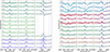 |
Fig. C.1. J1727 spectroscopic database showing the BAs evolution during the outburst, zoomed into the Balmer |


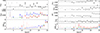 |
Fig. C.2. Best fitting parameters for the complete spectroscopic sample of J1727 (see Fig. C.1). The left figure contains parameters associated with the absorption component, while the right figure shows the emission component parameters. For those parameters that are independent for each of the fitted lines, the following colour code applies: |


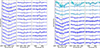 |
Fig. C.3. J1118 spectra from the 2000 (blue) and the 2005 outburst events (cyan). The best fit corresponding with the parameters shown in Fig. C.4 is shown as a solid blue line. Neither the DIB next to |


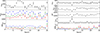 |
Fig. C.4. Best fitting parameters for the complete spectroscopic sample of J1118 (see Fig. C.3), following the same description as in Fig. C.2. |
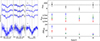 |
Fig. C.5. Left panel: J1753 spectra showing the BAs evolution during its 2023 outburst, zoomed into the Balmer |


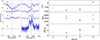 |
Fig. C.6. Left panel: J1357 spectra showing the BAs evolution during its 2011 outburst, zoomed into the Balmer |


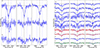 |
Fig. C.7. J1807 spectra from the 2017 (left) and 2023 (right) outburst events. The colour code mark the X-ray state, similarly to Fig. C.2. The best fit corresponding with the parameters compiled in Fig. C.8 is shown as a solid blue line. Neither the DIB next to |


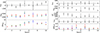 |
Fig. C.8. Best fitting parameters for the 2023 spectroscopic sample of J1807 (Fig. C.7), following the same description as in Fig. C.2. |
All Tables
All Figures
|
Fig. 1. Optical spectra from our database, zoomed in on the Balmer Hδ, Hγ, and Hβ transitions. They all show BAs with cores partially filled by the emission line. From bottom to top: J1807 (epoch 3 of dataset A, blue), J1727 (epoch 25, red), J1118 (epoch 1, green), and J1753 (epoch 2, magenta). Telluric bands and DIBs are shown as grey and yellow-shaded regions, respectively. The rest wavelength of the transition is marked with a dashed black line, while dotted blue lines mark velocity shifts of ±2500 km s−1 as a visual reference. |
| In the text | |
|
Fig. 2. b against Nepoch for the BH (left) and NS (right) population. Cyan symbols refer to systems with detected BA features (crosses for candidates, filled circles for confirmed systems), black symbols to non-BA systems (crosses for candidates, filled triangles for confirmed systems), and red dots to systems without available spectroscopic data (also known as uncharted). |
| In the text | |
|
Fig. 3. Porb against b for the BH (left) and NS (right) population. The colour and symbol description matches that of Fig. 2. The dashed black line marks the 11 h threshold described in the text. |
| In the text | |
|
Fig. 4. Porb against i for the BH population. The colour and symbol description matches that of Fig. 2. Dashed lines mark the thresholds at 30° and 60° that define the low, mid, and high inclination regions. If only constraints to the i parameter are available, we plot the central value and use the range as the associated uncertainty. |
| In the text | |
|
Fig. 5. Left panel: EWabs, Hδ against r-band brightness (left axis for flux density units, fν; right axis for absolute magnitudes, Mr) from the best-fitting results of the subsample with flux-calibrated spectra. The colour code marks the systems associated with each data point. A dashed black line depicts the best linear fit to the correlation, and dashed cyan, dashed red, and dashed black lines are the equivalent for individual datasets. Right panel: EWabs, Hβ against EWabs, Hγ from the best-fitting results of the whole spectroscopic sample. The colour code marks the systems associated with each data point, while symbols differentiate between subsets as described in the legend. A dashed black line depicts the best linear fit to the correlation, which is consistent with a 1:1 ratio. Transparent symbols correspond to fitting parameters that are consistent with null BA within 3σ. |
| In the text | |
|
Fig. 6. Histograms of the spectroscopic database for μabs, σabs, and EWabs (combining the results for Hβ and Hγ, which produced consistent distributions). The continuous and dashed black lines mark the mean and 1σ of the distribution, respectively. A Gaussian fit to the histogram is also shown as a red line. |
| In the text | |
|
Fig. 7. Schematic of the model for BA formation. The white cloud on top of the compact object is the illuminating X-ray source (e.g. the base of the jet or the corona). It emits both soft (cyan) and hard (black) X-ray photons. The former heats up the disc chromospheric region and gives rise to emission lines, while the later contributes to heating up deeper layers of the accretion disc. This produces a stellar-like temperature profile, with a relatively cold region on the surface producing the observed BAs. Note that the accretion disc also exhibits a radial gradient of temperature, so only the outermost rings develop such a region. |
| In the text | |
|
Fig. 8. Hardness-intensity diagram of J1727 (arrow-connected black dots; grey for low X-ray fluxes with colours possibly affected by background subtraction). The coloured symbols mark the epochs where our optical spectroscopy was obtained. The filled circles mark spectra where no BAs were detected, while filled stars correspond to BA detection in at least one of the inspected transitions (see Section 3). The colour code separates the initial rise in the hard state (blue), hard-intermediate state (HIMS, green), and soft-intermediate state (SIMS, orange), as well as the soft state decay (red). The last five epochs, published for the first time in this work, correspond to the final decay during the soft state and the subsequent transition to the low-luminosity hard state (cyan). |
| In the text | |
|
Fig. C.1. J1727 spectroscopic database showing the BAs evolution during the outburst, zoomed into the Balmer |
| In the text | |
|
Fig. C.2. Best fitting parameters for the complete spectroscopic sample of J1727 (see Fig. C.1). The left figure contains parameters associated with the absorption component, while the right figure shows the emission component parameters. For those parameters that are independent for each of the fitted lines, the following colour code applies: |
| In the text | |
|
Fig. C.3. J1118 spectra from the 2000 (blue) and the 2005 outburst events (cyan). The best fit corresponding with the parameters shown in Fig. C.4 is shown as a solid blue line. Neither the DIB next to |
| In the text | |
|
Fig. C.4. Best fitting parameters for the complete spectroscopic sample of J1118 (see Fig. C.3), following the same description as in Fig. C.2. |
| In the text | |
|
Fig. C.5. Left panel: J1753 spectra showing the BAs evolution during its 2023 outburst, zoomed into the Balmer |
| In the text | |
|
Fig. C.6. Left panel: J1357 spectra showing the BAs evolution during its 2011 outburst, zoomed into the Balmer |
| In the text | |
|
Fig. C.7. J1807 spectra from the 2017 (left) and 2023 (right) outburst events. The colour code mark the X-ray state, similarly to Fig. C.2. The best fit corresponding with the parameters compiled in Fig. C.8 is shown as a solid blue line. Neither the DIB next to |
| In the text | |
|
Fig. C.8. Best fitting parameters for the 2023 spectroscopic sample of J1807 (Fig. C.7), following the same description as in Fig. C.2. |
| In the text | |
Current usage metrics show cumulative count of Article Views (full-text article views including HTML views, PDF and ePub downloads, according to the available data) and Abstracts Views on Vision4Press platform.
Data correspond to usage on the plateform after 2015. The current usage metrics is available 48-96 hours after online publication and is updated daily on week days.
Initial download of the metrics may take a while.