| Issue |
A&A
Volume 708, April 2026
|
|
|---|---|---|
| Article Number | A179 | |
| Number of page(s) | 25 | |
| Section | Astrophysical processes | |
| DOI | https://doi.org/10.1051/0004-6361/202556759 | |
| Published online | 08 April 2026 | |
Full-polarization millimeter wavelength variability of Sagittarius A* during the 2018 EHT campaign
1
Massachusetts Institute of Technology Haystack Observatory, 99 Millstone Road, Westford, MA 01886, USA
2
National Astronomical Observatory of Japan, 2-21-1 Osawa, Mitaka, Tokyo 181-8588, Japan
3
Black Hole Initiative at Harvard University, 20 Garden Street, Cambridge, MA 02138, USA
4
Departament d’Astronomia i Astrofísica, Universitat de València, C. Dr. Moliner 50, E-46100 Burjassot, València, Spain
5
Instituto de Astrofísica de Andalucía-CSIC, Glorieta de la Astronomía s/n, E-18008 Granada, Spain
6
Max-Planck-Institut für Radioastronomie, Auf dem Hügel 69, D-53121 Bonn, Germany
7
Department of Physics, Faculty of Science, Universiti Malaya, 50603 Kuala Lumpur, Malaysia
8
Department of Physics & Astronomy, The University of Texas at San Antonio, One UTSA Circle, San Antonio, TX 78249, USA
9
Physics & Astronomy Department, Rice University, Houston, TX 77005-1827, USA
10
Center for Astrophysics | Harvard & Smithsonian, 60 Garden Street, Cambridge, MA 02138, USA
11
Institute of Astronomy and Astrophysics, Academia Sinica, 11F of Astronomy-Mathematics Building, AS/NTU No. 1, Sec. 4, Roosevelt Rd., Taipei 106216, Taiwan, ROC
12
Observatori Astronómic, Universitat de València, C. Catedrático José Beltrán 2, E-46980 Paterna, València, Spain
13
Department of Space, Earth and Environment, Chalmers University of Technology, Onsala Space Observatory, SE-43992 Onsala, Sweden
14
Steward Observatory and Department of Astronomy, University of Arizona, 933 N. Cherry Ave., Tucson, AZ 85721, USA
15
Yale Center for Astronomy & Astrophysics, Yale University, 52 Hillhouse Avenue, New Haven, CT 06511, USA
16
Astronomy Department, Universidad de Concepción, Casilla 160-C, Concepción, Chile
17
Department of Physics, University of Illinois, 1110 West Green Street, Urbana, IL 61801, USA
18
Fermi National Accelerator Laboratory, MS209, P.O. Box 500 Batavia, IL 60510, USA
19
Department of Astronomy and Astrophysics, University of Chicago, 5640 South Ellis Avenue, Chicago, IL 60637, USA
20
East Asian Observatory, 660 N. A’ohoku Place, Hilo, HI 96720, USA
21
James Clerk Maxwell Telescope (JCMT), 660 N. A’ohoku Place, Hilo, HI 96720, USA
22
California Institute of Technology, 1200 East California Boulevard, Pasadena, CA 91125, USA
23
Department of Physics and Astronomy, University of Hawaii at Manoa, 2505 Correa Road, Honolulu, HI 96822, USA
24
Institut de Radioastronomie Millimétrique (IRAM), 300 rue de la Piscine, F-38406 Saint Martin d’Hères, France
25
Perimeter Institute for Theoretical Physics, 31 Caroline Street North, Waterloo, ON N2L 2Y5, Canada
26
Department of Physics and Astronomy, University of Waterloo, 200 University Avenue West, Waterloo, ON N2L 3G1, Canada
27
Waterloo Centre for Astrophysics, University of Waterloo, Waterloo, ON N2L 3G1, Canada
28
Department of Astrophysics, Institute for Mathematics, Astrophysics and Particle Physics (IMAPP), Radboud University, P.O. Box 9010, 6500 GL, Nijmegen, The Netherlands
29
Department of Astronomy, University of Massachusetts, Amherst, MA 01003, USA
30
Instituto de Astronomia, Geofísica e Ciências Atmosféricas, Universidade de São Paulo, R. do Matão, 1226 São Paulo, SP 05508-090, Brazil
31
Kavli Institute for Cosmological Physics, University of Chicago, 5640 South Ellis Avenue, Chicago, IL 60637, USA
32
Department of Physics, University of Chicago, 5720 South Ellis Avenue, Chicago, IL 60637, USA
33
Enrico Fermi Institute, University of Chicago, 5640 South Ellis Avenue, Chicago, IL 60637, USA
34
Princeton Gravity Initiative, Jadwin Hall, Princeton University, Princeton, NJ 08544, USA
35
Data Science Institute, University of Arizona, 1230 N. Cherry Ave., Tucson, AZ 85721, USA
36
Program in Applied Mathematics, University of Arizona, 617 N. Santa Rita, Tucson, AZ 85721, USA
37
Cornell Center for Astrophysics and Planetary Science, Cornell University, Ithaca, NY 14853, USA
38
Institute of Astronomy and Astrophysics, Academia Sinica, 645 N. A’ohoku Place, Hilo, HI 96720, USA
39
Shanghai Astronomical Observatory, Chinese Academy of Sciences, 80 Nandan Road, Shanghai 200030, PR China
40
Key Laboratory of Radio Astronomy and Technology, Chinese Academy of Sciences, A20 Datun Road, Chaoyang District, Beijing 100101, PR China
41
Korea Astronomy and Space Science Institute, Daedeok-daero 776, Yuseong-gu, Daejeon 34055, Republic of Korea
42
Department of Astronomy, Yonsei University, Yonsei-ro 50, Seodaemun-gu, 03722 Seoul, Republic of Korea
43
WattTime, 490 43rd Street, Unit 221 Oakland, CA 94609, USA
44
Department of Astronomy, University of Illinois at Urbana-Champaign, 1002 West Green Street, Urbana, IL 61801, USA
45
Instituto de Astronomía, Universidad Nacional Autónoma de México (UNAM), Apdo Postal 70-264 Ciudad de México, Mexico
46
Institut für Theoretische Physik, Goethe-Universität Frankfurt, Max-von-Laue-Straße 1, D-60438 Frankfurt am Main, Germany
47
Institute of Astrophysics, Central China Normal University, Wuhan 430079, PR China
48
Department of Astrophysical Sciences, Peyton Hall, Princeton University, Princeton, NJ 08544, USA
49
NASA Hubble Fellowship Program, Einstein Fellow
50
Dipartimento di Fisica “E. Pancini”, Università di Napoli “Federico II”, Compl. Univ. di Monte S. Angelo, Edificio G, Via Cinthia, I-80126 Napoli, Italy
51
INFN Sez. di Napoli, Compl. Univ. di Monte S. Angelo, Edificio G, Via Cinthia, I-80126 Napoli, Italy
52
Wits Centre for Astrophysics, University of the Witwatersrand, Braamfontein, Johannesburg 2050, South Africa
53
Department of Physics, University of Pretoria, Hatfield, Pretoria 0028, South Africa
54
Centre for Radio Astronomy Techniques and Technologies, Department of Physics and Electronics, Rhodes University, Makhanda 6140, South Africa
55
ASTRON, Oude Hoogeveensedijk 4, 7991 PD, Dwingeloo, The Netherlands
56
LESIA, Observatoire de Paris, Université PSL, CNRS, Sorbonne Université, Université de Paris, 5 place Jules Janssen, F-92195 Meudon, France
57
JILA and Department of Astrophysical and Planetary Sciences, University of Colorado, Boulder, CO 80309, USA
58
Tsung-Dao Lee Institute, Shanghai Jiao Tong University, Shengrong Road 520, Shanghai 201210, PR China
59
National Astronomical Observatories, Chinese Academy of Sciences, 20A Datun Road, Chaoyang District, Beijing 100101, PR China
60
Las Cumbres Observatory, 6740 Cortona Drive, Suite 102 Goleta, CA 93117-5575, USA
61
Department of Physics, University of California, Santa Barbara, CA 93106-9530, USA
62
National Radio Astronomy Observatory, 520 Edgemont Road, Charlottesville, USA
63
Department of Electrical Engineering and Computer Science, Massachusetts Institute of Technology, 32-D476, 77 Massachusetts Ave., Cambridge, MA 02142, USA
64
Google Research, 355 Main St., Cambridge, MA 02142, USA
65
Institut für Theoretische Physik und Astrophysik, Universität Würzburg, Emil-Fischer-Str. 31 Würzburg, 97074, Germany
66
Department of History of Science, Harvard University, Cambridge, MA 02138, USA
67
Department of Physics, Harvard University, Cambridge, MA 02138, USA
68
NCSA, University of Illinois, 1205 W. Clark St., Urbana, IL 61801, USA
69
Royal Netherlands Meteorological Institute, Utrechtseweg 297, 3731 GA, De Bilt, The Netherlands
70
Dipartimento di Fisica, Università degli Studi di Cagliari, SP Monserrato-Sestu km 0.7, I-09042 Monserrato (CA), Italy
71
INAF – Osservatorio Astronomico di Cagliari, via della Scienza 5, I-09047 Selargius (CA), Italy
72
INFN, sezione di Cagliari, I-09042 Monserrato (CA), Italy
73
Institute for Mathematics and Interdisciplinary Center for Scientific Computing, Heidelberg University, Im Neuenheimer Feld 205, Heidelberg 69120, Germany
74
Institut für Theoretische Physik, Universität Heidelberg, Philosophenweg 16, 69120 Heidelberg, Germany
75
CP3-Origins, University of Southern Denmark, Campusvej 55, DK-5230 Odense, Denmark
76
Instituto Nacional de Astrofísica, Óptica y Electrónica. Apartado Postal 51 y 216, 72000, Puebla Pue., Mexico
77
Consejo Nacional de Humanidades, Ciencia y Tecnología, Av. Insurgentes Sur 1582, 03940 Ciudad de México, Mexico
78
Key Laboratory for Research in Galaxies and Cosmology, Chinese Academy of Sciences, Shanghai 200030, PR China
79
Graduate School of Science, Nagoya City University, Yamanohata 1, Mizuho-cho, Mizuho-ku, Nagoya 467-8501, Aichi, Japan
80
Mizusawa VLBI Observatory, National Astronomical Observatory of Japan, 2-12 Hoshigaoka, Mizusawa, Oshu, Iwate 023-0861, Japan
81
Department of Physics, McGill University, 3600 rue University, Montréal, QC H3A 2T8, Canada
82
Trottier Space Institute at McGill, 3550 rue University, Montréal, QC H3A 2A7, Canada
83
NOVA Sub-mm Instrumentation Group, Kapteyn Astronomical Institute, University of Groningen, Landleven 12, 9747 AD, Groningen, The Netherlands
84
Department of Astronomy, School of Physics, Peking University, Beijing 100871, PR China
85
Kavli Institute for Astronomy and Astrophysics, Peking University, Beijing 100871, PR China
86
Department of Astronomical Science, The Graduate University for Advanced Studies (SOKENDAI), 2-21-1 Osawa, Mitaka, Tokyo 181-8588, Japan
87
Department of Astronomy, Graduate School of Science, The University of Tokyo, 7-3-1 Hongo, Bunkyo-ku, Tokyo 113-0033, Japan
88
The Institute of Statistical Mathematics, 10-3 Midori-cho, Tachikawa, Tokyo 190-8562, Japan
89
Department of Statistical Science, The Graduate University for Advanced Studies (SOKENDAI), 10-3 Midori-cho, Tachikawa, Tokyo 190-8562, Japan
90
Kavli Institute for the Physics and Mathematics of the Universe, The University of Tokyo, 5-1-5 Kashiwanoha, Kashiwa 277-8583, Japan
91
Leiden Observatory, Leiden University, Postbus 2300, 9513 RA, Leiden, The Netherlands
92
ASTRAVEO LLC, PO Box 1668 Gloucester, MA 01931, USA
93
Applied Materials Inc., 35 Dory Road, Gloucester, MA 01930, USA
94
Institute for Astrophysical Research, Boston University, 725 Commonwealth Ave., Boston, MA 02215, USA
95
University of Science and Technology, Gajeong-ro 217, Yuseong-gu, Daejeon 34113, Republic of Korea
96
Institute for Cosmic Ray Research, The University of Tokyo, 5-1-5 Kashiwanoha, Kashiwa, Chiba 277-8582, Japan
97
Joint Institute for VLBI ERIC (JIVE), Oude Hoogeveensedijk 4, 7991 PD, Dwingeloo, The Netherlands
98
CSIRO, Space and Astronomy, PO Box 76 Epping, NSW 1710, Australia
99
Department of Physics, Ulsan National Institute of Science and Technology (UNIST), Ulsan 44919, Republic of Korea
100
Department of Physics, Korea Advanced Institute of Science and Technology (KAIST), 291 Daehak-ro, Yuseong-gu, Daejeon 34141, Republic of Korea
101
Kogakuin University of Technology & Engineering, Academic Support Center, 2665-1 Nakano, Hachioji, Tokyo 192-0015, Japan
102
Graduate School of Science and Technology, Niigata University, 8050 Ikarashi 2-no-cho, Nishi-ku, Niigata 950-2181, Japan
103
Physics Department, National Sun Yat-Sen University, No. 70, Lien-Hai Road, Kaosiung City, 80424, Taiwan, ROC
104
School of Astronomy and Space Science, Nanjing University, Nanjing 210023, PR China
105
Key Laboratory of Modern Astronomy and Astrophysics, Nanjing University, Nanjing 210023, PR China
106
Common Crawl Foundation, 9663 Santa Monica Blvd. 425 Beverly Hills, CA 90210, USA
107
Instituto de Física, Pontificia Universidad Católica de Valparaíso, Casilla 4059 Valparaíso, Chile
108
INAF-Istituto di Radioastronomia & Italian ALMA Regional Centre, Via P. Gobetti 101, I-40129 Bologna, Italy
109
Department of Physics, National Taiwan University, No. 1, Sec. 4, Roosevelt Rd., Taipei 106216, Taiwan, ROC
110
Instituto de Radioastronomía y Astrofísica, Universidad Nacional Autónoma de México, Morelia 58089, Mexico
111
David Rockefeller Center for Latin American Studies, Harvard University, 1730 Cambridge Street, Cambridge, MA 02138, USA
112
Yunnan Observatories, Chinese Academy of Sciences, 650011 Kunming, Yunnan Province, PR China
113
Center for Astronomical Mega-Science, Chinese Academy of Sciences, 20A Datun Road, Chaoyang District, Beijing 100012, PR China
114
Key Laboratory for the Structure and Evolution of Celestial Objects, Chinese Academy of Sciences, 650011 Kunming, PR China
115
Anton Pannekoek Institute for Astronomy, University of Amsterdam, Science Park 904, 1098 XH, Amsterdam, The Netherlands
116
Gravitation and Astroparticle Physics Amsterdam (GRAPPA) Institute, University of Amsterdam, Science Park 904, 1098 XH, Amsterdam, The Netherlands
117
School of Physics and Astronomy, Shanghai Jiao Tong University, Shanghai, PR China
118
Institut de Radioastronomie Millimétrique (IRAM), Avenida Divina Pastora 7, Local 20, E-18012 Granada, Spain
119
National Institute of Technology, Hachinohe College, 16-1 Uwanotai, Tamonoki, Hachinohe City, Aomori 039-1192, Japan
120
Research Center for Astronomy, Academy of Athens, Soranou Efessiou 4, 115 27 Athens, Greece
121
Department of Physics, Villanova University, 800 Lancaster Avenue, Villanova, PA 19085, USA
122
Physics Department, Washington University, CB 1105, St. Louis, MO 63130, USA
123
Departamento de Matemática da Universidade de Aveiro and Centre for Research and Development in Mathematics and Applications (CIDMA), Campus de Santiago, 3810-193 Aveiro, Portugal
124
School of Physics, Georgia Institute of Technology, 837 State St NW, Atlanta, GA 30332, USA
125
School of Space Research, Kyung Hee University, 1732, Deogyeong-daero, Giheung-gu, Yongin-si, Gyeonggi-do, 17104, Republic of Korea
126
Canadian Institute for Theoretical Astrophysics, University of Toronto, 60 St. George Street, Toronto, ON M5S 3H8, Canada
127
Dunlap Institute for Astronomy and Astrophysics, University of Toronto, 50 St. George Street, Toronto, ON M5S 3H4, Canada
128
Canadian Institute for Advanced Research, 180 Dundas St West, Toronto, ON M5G 1Z8, Canada
129
Dipartimento di Fisica, Università di Trieste, I-34127 Trieste, Italy
130
INFN Sez. di Trieste, I-34127 Trieste, Italy
131
Department of Physics, National Taiwan Normal University, No. 88, Sec. 4, Tingzhou Rd., Taipei 116, Taiwan, ROC
132
Center of Astronomy and Gravitation, National Taiwan Normal University, No. 88, Sec. 4, Tingzhou Road, Taipei 116, Taiwan, ROC
133
Finnish Centre for Astronomy with ESO, University of Turku, FI-20014 Turun Yliopisto, Finland
134
Aalto University Metsähovi Radio Observatory, Metsähovintie 114, FI-02540 Kylmälä, Finland
135
Gemini Observatory/NSF NOIRLab, 670 N. A’ohōkū Place, Hilo, HI 96720, USA
136
Frankfurt Institute for Advanced Studies, Ruth-Moufang-Strasse 1, D-60438 Frankfurt, Germany
137
School of Mathematics, Trinity College, Dublin 2, Ireland
138
Department of Physics, University of Toronto, 60 St. George Street, Toronto, ON M5S 1A7, Canada
139
Department of Physics, Tokyo Institute of Technology, 2-12-1 Ookayama, Meguro-ku, Tokyo 152-8551, Japan
140
Hiroshima Astrophysical Science Center, Hiroshima University, 1-3-1 Kagamiyama, Higashi-Hiroshima, Hiroshima 739-8526, Japan
141
Aalto University Department of Electronics and Nanoengineering, PL 15500, FI-00076 Aalto, Finland
142
Jeremiah Horrocks Institute, University of Central Lancashire, Preston PR1 2HE, UK
143
National Biomedical Imaging Center, Peking University, Beijing 100871, PR China
144
College of Future Technology, Peking University, Beijing 100871, PR China
145
Tokyo Electron Technology Solutions Limited, 52 Matsunagane, Iwayado, Esashi, Oshu, Iwate 023-1101, Japan
146
Department of Physics and Astronomy, University of Lethbridge, Lethbridge, Alberta T1K 3M4, Canada
147
Netherlands Organisation for Scientific Research (NWO), Postbus 93138, 2509 AC, Den Haag, The Netherlands
148
Frontier Research Institute for Interdisciplinary Sciences, Tohoku University, Sendai 980-8578, Japan
149
Astronomical Institute, Tohoku University, Sendai 980-8578, Japan
150
Department of Physics and Astronomy, Seoul National University, Gwanak-gu, Seoul 08826, Republic of Korea
151
SNU Astronomy Research Center, Seoul National University, Gwanak-gu, Seoul 08826, Republic of Korea
152
University of New Mexico, Department of Physics and Astronomy, Albuquerque, NM 87131, USA
153
Physics Department, Brandeis University, 415 South Street, Waltham, MA 02453, USA
154
Tuorla Observatory, Department of Physics and Astronomy, University of Turku, FI-20014 Turun Yliopisto, Finland
155
Radboud Excellence Fellow of Radboud University, Nijmegen, The Netherlands
156
School of Natural Sciences, Institute for Advanced Study, 1 Einstein Drive, Princeton, NJ 08540, USA
157
School of Physics, Huazhong University of Science and Technology, Wuhan, Hubei 430074, PR China
158
Mullard Space Science Laboratory, University College London, Holmbury St. Mary, Dorking, Surrey RH5 6NT, UK
159
Center for Astronomy and Astrophysics and Department of Physics, Fudan University, Shanghai 200438, PR China
160
Astronomy Department, University of Science and Technology of China, Hefei 230026, PR China
161
Department of Physics and Astronomy, Michigan State University, 567 Wilson Rd, East Lansing, MI 48824, USA
★ Corresponding author.
Received:
5
August
2025
Accepted:
18
November
2025
Abstract
Context. Sagittarius A* (Sgr A*), the supermassive black hole at the center of the Milky Way, provides a unique laboratory to study accretion dynamics and plasma processes near the event horizon.
Aims. We investigated the variability and polarization properties of Sgr A* using ALMA observations during the 2018 Event Horizon Telescope campaign.
Methods. We analyzed high-cadence full-polarization light curves from ALMA at millimeter wavelengths, performed time-series analysis, and investigated the temporal behavior during an X-ray flare observed by Chandra on 2018 April 24. The variability characteristics are compared with expectations from standard accretion flow models.
Results. We find low variability in total intensity (σ/μ < 10%), but significantly higher variability in linear and circular polarization (∼30% and ∼50%, respectively). A time-series analysis reveals red-noise variability, with power spectral densities between −2 and −3 across all Stokes parameters. Polarized intensity shows stable intra-day timescales, while total intensity exhibits more variable timescales, suggesting distinct emission regions, with polarization likely arising from a coherent structure. On April 24, a statistically significant inter-band delay in polarized intensity coincides with a near-simultaneous X-ray and millimeter peak that deviates from the typical delayed flare scenario. This event also features enhanced millimeter variability and coherent polarization loop evolution. The observed simultaneity challenges standard models of transient synchrotron emission with cooling delays, favoring instead a scenario of continuous energy injection in an optically thin region.
Conclusions. Our results offer new constraints on the physical mechanisms driving variability in Sgr A*, and provide key observational input for refining theoretical models of accretion and plasma behavior in the vicinity of supermassive black holes.
Key words: black hole physics / techniques: interferometric / techniques: polarimetric / Galaxy: center
© The Authors 2026
 Open Access article, published by EDP Sciences, under the terms of the Creative Commons Attribution License (https://creativecommons.org/licenses/by/4.0), which permits unrestricted use, distribution, and reproduction in any medium, provided the original work is properly cited.
This article is published in open access under the Subscribe to Open model. This email address is being protected from spambots. You need JavaScript enabled to view it. to support open access publication.
1. Introduction
The Galactic center (GC) is one of the most extensively studied astrophysical environments, hosting a rich and diverse population of radio sources (Heywood et al. 2022). At the heart of the GC lies Sagittarius A* (Sgr A*; Balick & Brown 1974), a supermassive black hole with a mass of approximately 4 × 10⁶ M⊙ (Do et al. 2019; GRAVITY Collaboration 2022; Event Horizon Telescope Collaboration 2022a). This source exhibits significant variability at radio frequencies (Brown & Lo 1982; Iwata et al. 2020; Wielgus et al. 2022a; Mus et al. 2022), with spatial variations in its emission structure observable on timescales shorter than 30 minutes (GRAVITY Collaboration 2018, 2023).
Particularly striking are the intense flare events detected in the near-infrared (NIR) and X-ray regimes in the vicinity of Sgr A* (Genzel et al. 2003; Aschenbach et al. 2004; Eckart et al. 2006; Boyce et al. 2019). These flares are thought to result from magnetic reconnection events, which dissipate magnetic energy and may produce transient features such as orbiting hot spots of plasma (Yuan et al. 2003; Dexter et al. 2020; Porth et al. 2021; Ripperda et al. 2022; Wielgus et al. 2022b).
Multiwavelength studies of Sgr A*’s variability have provided valuable insights into its radiation mechanisms and spatial emission regions. Simultaneous X-ray and infrared (IR) flares suggest that these emissions predominantly originate from the same regions, with delays of approximately 10–20 minutes between the two wavebands (Eckart et al. 2004; Marrone et al. 2008; Boyce et al. 2019). In contrast, millimeter and submillimeter flares show more complex behavior, with reported delays, relative to NIR and X-ray emissions, ranging from 20–30 minutes (Marrone et al. 2008; Witzel et al. 2021) to several hours (Yusef-Zadeh et al. 2008; Eckart et al. 2012; Event Horizon Telescope Collaboration 2022b). Some studies have even reported minimal or negligible delays between millimeter and IR/X-ray flares (Fazio et al. 2018), or have suggested that previously perceived delays may have been coincidental (Capellupo et al. 2017). This inconsistency underscores the need for high-fidelity millimeter light curves, which have recently become accessible through advanced facilities such as the Atacama Large Millimeter/Submillimeter Array (ALMA) and the Submillimeter Array (SMA; Bower et al. 2015; Witzel et al. 2021).
During the first Event Horizon Telescope (EHT) observing campaign in April 2017, millimeter light curves of Sgr A* were obtained from both ALMA and SMA, as reported by Wielgus et al. (2022a). On April 11, 2017, an X-ray flare was detected by Chandra (Event Horizon Telescope Collaboration 2022b), providing a unique opportunity to investigate the effect of an X-ray flare on millimeter-wavelength light curves. While the light curves from April 6 and 7, 2017, exhibited a low-variability state, the April 11 light curve showed pronounced variability following the X-ray flare.
Beyond total intensity, the exceptional sensitivity of ALMA has also enabled detailed studies of the polarimetric properties of Sgr A* and other active galactic nuclei (AGN) during the 2017 Very Long Baseline Interferometry (VLBI) campaign (Goddi et al. 2021). Polarization measurements offer a powerful, time-resolved probe of the emission and propagation processes in Sgr A*, complementing the spatially resolved Event Horizon Telescope (EHT) analysis (Event Horizon Telescope Collaboration 2024; Joshi et al. 2024). Although Sgr A* is powered by a radiatively inefficient accretion flow (Yuan & Narayan 2014), fundamental properties such as magnetic field geometry, plasma composition, and turbulence remain poorly constrained. Unlike total intensity, polarization encodes information about magnetic field structure, Faraday rotation, optical depth, and the nature of the emitting electrons (e.g., Macquart et al. 2006; Johnson et al. 2015; Wielgus et al. 2024). In particular, variations in polarization degree and angle constrain several physical properties: the viewing geometry (axisymmetric fields tend to depolarize when seen face-on; e.g., Shcherbakov et al. 2012), the magnetic field strength, number density and temperature of electrons through the Faraday depth (Quataert & Gruzinov 2000; Wielgus et al. 2024), and turbulence in the accretion flow (Bower et al. 2005). ALMA observations have revealed hour- to month-scale variability in linear polarization and persistent circular polarization, consistent with Faraday conversion in an ordered field (Bower et al. 2018). Temporal features, such as polarization angle swings, depolarization dips, or Q–U loops, provide further diagnostics to distinguish between accretion scenarios, with magnetically arrested disk (MAD) models predicting strong organized fields, and standard and normal evolution (SANE) models favoring weaker turbulent configurations. Moreover, frequency-dependent polarization delays constrain the optical depth and cooling timescales of the emitting plasma (Wielgus et al. 2022b; Michail et al. 2024).
The polarimetric variability observed in Sgr A* after the X-ray flare detected on April 11, 2017, suggests the presence of orbital motion of a hot spot near the black hole following a high-energy flare (Wielgus et al. 2022b), consistent with earlier findings by GRAVITY (GRAVITY Collaboration 2018, 2020). More recently, Wielgus et al. (2024) conducted a joint analysis of polarized light curves of Sgr A* at 85–101 GHz and 212–230 GHz with ALMA, revealing insights into inefficient accretion flows and an internal Faraday screen through the analysis of rotation measure (RM) and its variability. These results imply that a significant fraction of Faraday rotation occurs in the compact source near the event horizon, and that the magnetic field on this scale is organized and not violently variable.
Building upon these findings, for this work we analyzed Sgr A*’s millimeter light curves obtained from ALMA and SMA observations during the second EHT observing campaign in April 2018, covering four observing days: April 21, 22, 24, and 25. We investigated the full-polarization variability by characterizing and comparing the light curves from the 2017 and 2018 campaigns using time-series analysis techniques. Similarly to April 11, 2017, an X-ray flare was detected by Chandra on April 24, 2018 (Mossoux et al. 2020), coinciding with ALMA coverage. Therefore, in addition to the full-polarization variability of Sgr A*’s light curves, we closely examined this flare event, assessed its imprint on the millimeter light curves, and compared our findings with those from 2017.
This paper is structured as follows. Section 2 describes the observations and details the data reduction procedures implemented to recover the compact source emission variability from ALMA data. In Sect. 3 we present the full-polarization ALMA light curves and compare them with historical data. Section 4 details the complete time-variability analysis of the 2017 and 2018 light curves. In Sect. 5 we discuss specific properties of the light curves, highlighting persistent clockwise Q–U rotation, accretion physics, and X-ray flaring, and compare the variability with GRMHD predictions. Finally, we summarize our conclusions in Sect. 6.
2. Observations and data calibration
2.1. ALMA observations and data processing
Sgr A* was observed with phased-ALMA (Matthews et al. 2018; Crew et al. 2023) on April 21, 22, 24, and 25 as part of the 2018 EHT+ALMA campaign. A detailed analysis of the EHT VLBI observations of Sgr A* in 2018 will be presented elsewhere (EHT Collaboration, in prep.). The VLBI observations were carried out while the array was in its most compact configurations and only antennas within a radius of 180 m (from the array center) were used for phasing. The observations were performed in full-polarization mode in order to supply the inputs to the polarization conversion process at the VLBI correlators (Martí-Vidal et al. 2016).
The spectral setup included four spectral windows (SPWs) of 1875 MHz, two in the lower and two in the upper sideband, centered at 213.1, 215.1, 227.1, and 229.1 GHz. Table E.1 summarizes the observational and spectral setup of the April 2018 observations, including four tracks (which ranged from roughly 6 to 9 hours). An absorption feature in the SPW centered at 227.1 GHz was flagged to ensure consistency in the Sgr A* light curves (see Appendix A).
ALMA data acquired during VLBI observations are calibrated using the Common Astronomy Software Applications (CASA) package (The CASA Team et al. 2022) and the special procedures known as “Quality Assurance Level 2” (QA2) described in Goddi et al. (2019). Bandpass solutions were obtained using 3C 279, which also served as the polarization calibrator on all four observing days. Flux calibration was performed using Titan on April 21 and 25, and 3C 279 on April 22 and 24. To evaluate the accuracy of our flux-density calibration, we compared the QA2-derived fluxes of VLBI targets with independent Atacama Compact Array (ACA) flux monitoring of Grid Sources, some of which overlap with our VLBI sample. The analysis shows that ALMA fluxes during VLBI observations agree within 10% in Band 6, consistent with ALMA’s nominal absolute calibration uncertainty (Remijan et al. 2019). This result aligns with similar findings reported in Goddi et al. (2021, 2025) for VLBI observations in Bands 6 and 7.
The QA2 process relies on self-calibration under the assumption of a point source with constant flux density. This approach is effective for most VLBI targets, which are generally stable over the course of an observation. As shown in Appendix B, the visibility amplitude light curves of both the calibrators and EHT targets confirm this flux stability. However, this method is not well suited for Sgr A*, which exhibits intrinsic variability on minute timescales. In the following, we describe the specialized procedure required to calibrate a time-variable source like Sgr A* accurately.
2.2. Intra-field calibration of Sgr A*
Sgr A* can be understood as the sum of two components (shown in Fig. 1):
-
An extended component (up to parsec scales), hereby called the minispiral. Given its large extension, it is safe to assume that this component is not variable on the timescales comparable to the duration of the observations (i.e., a few hours).
-
A compact, bright component, which presents high variability: Sgr A* itself.
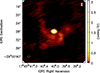 |
Fig. 1. Stokes I CLEAN image of Sgr A* and the minispiral from visibilities at 213.1 GHz, produced after the QA2 calibration for April 21. |
The assumption of constant flux density in the QA2 calibration results in a core with constant brightness, shifting all variability to the minispiral. To derive the light curves of Sgr A* (i.e., the compact core), we implemented an algorithm to enhance the QA2 gain calibration for variable sources, building upon previous work presented in Wielgus et al. (2022a), Mus et al. (2022)1. Here we summarize the main procedure, consisting of four steps:
-
Generate a CLEAN image of the source (i.e., the core and the minispiral), labeled as IM0. Although including artifacts (e.g., negative features simulating partial sidelobes of the PSF around Sgr A*), this image serves as an initial model for the minispiral.
-
Subtract the core of Sgr A* from the IM0 image by setting the flux of the pixels corresponding to the compact component to zero, producing an image of only the minispiral (IM1).
-
Visibility (two-component) model fitting: Construct a Visibility model as the Fourier transform of the minispiral (MOD = FT(IM1)) scaled by a time-varying factor S1 (which accounts for the minispiral’s artificial variability introduced by QA2) and a constant factor S2 (core flux density)2, thus describing the entire structure of Sgr A*:
 (1)
(1)For each integration time t, we fit the observed visibilities to our model by minimizing the χ2 function
 (2)
(2)where ωi are the weights of each visibility.
-
Transfer the variability from S1 to S2 by scaling the Sgr A* light curves as
 (3)
(3)where VQA2 represents the QA2 visibilities, Vcal(t) are the calibrated visibilities, and
 is the median of all minispiral flux densities across all days of the campaign.
This algorithm corrects the amplitude of all visibilities for each integration time, ensuring that the minispiral brightness remains nearly constant (within ≲1%), while allowing the core to exhibit the expected flux density variability, as illustrated in Fig. 2. A final round of flagging is typically performed to remove data points that vary significantly between consecutive time intervals, as detailed in Sect. 3.1.
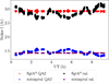 |
Fig. 2. April 22 total flux density of Sgr A* and the minispiral at 213.1 GHz, before (red and blue crosses) and after (purple and black dots) correcting for variability transfer. The flux density uncertainty, estimated from the covariance matrix, is approximately 0.1% and is therefore not visible. |
A complementary calibration method for the time-variable source Sgr A* is presented in Appendix C, where the manual reduction of the ALMA data is described in detail. Additionally, in Appendix D we present the SMA observations and data calibration, and compare the resulting light curves of Sgr A* with those from ALMA as a consistency test.
3. Sgr A* full-polarization variability
3.1. ALMA light curves
Following the intra-field calibration of the ALMA data, presented in Sect. 2.2, we retrieved the full-polarization Sgr A* light curves with a 4 second cadence, which will be analyzed in the following sections3. To remove outliers, we fit the Stokes I light curves with a fifth-order spline function and discard data points deviating beyond a 3σ threshold. Due to the higher noise in the April 25 light curve, we averaged the data over 16-second intervals, matching the timing of the ALMA phasing loop (Goddi et al. 2019), to mitigate its impact.
The ALMA light curves for the four observing days are presented in Appendix E (Table E.1) and plotted in Figs. 3 and 4. Table E.1 summarizes the main variability characteristics of Sgr A*, reporting for each of the four ALMA spectral windows the average and dispersion of three parameters: total intensity (Stokes I), polarized intensity  , and Stokes V. Variability is quantified using the modulation index, defined as the ratio of the standard deviation to the mean. The numerical values are listed in Table E.1. Comparing the modulation indices of the Stokes I light curves with those of the polarized intensity reveals a difference of an order of magnitude, suggesting significantly greater variability in polarization than in total flux density. This behavior is also evident in Fig. 3, which shows the time evolution of total flux density, polarized intensity, polarization angle (EVPA; defined as ϕ = 0.5arg(Q + iU)), and Stokes V across the four observing nights.
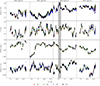 |
Fig. 3. Sgr A* ALMA light curves of Stokes I, the polarized intensity, the EVPA, and Stokes V (from top to bottom) for the four spectral bands, for all four days (from left to right, April 21, 22, 24, and 25). Stokes V light curves are tentative, as the detected levels fall below ALMA’s guaranteed CP accuracy. The gray-shaded band on April 24 marks the time range of the Chandra X-ray flare. |
While the Stokes V light curve is predominantly negative, consistent with previous studies (Marrone et al. 2006; Bower et al. 2018; Wielgus et al. 2022b), the average amplitude of the circular polarization is around 1% of the total flux, well below the ALMA’s nominal 3σ detection threshold of 1.8%. In this dataset, calibration was performed using 3C279, whose intrinsic circular polarization is unknown. As a result, any true Stokes V signal from the calibrator may be absorbed into instrumental terms and subsequently imprinted onto the target source as an artificial signal. In light of these limitations, we do not attempt to analyze the Stokes V data. A dedicated investigation of the circular polarization, following the approach of Goddi et al. (2021, Appendix G), is planned for a future publication.
Figure 4 presents four additional parameters: the fractional linear polarization m = P/I (LP), the Depolarization Measure (m′), the Rotation Measure (RM), and the Spectral Index α. The RM is defined by the relation ϕ(λ) = ϕ0 + RM(λ2 − λ02) (e.g., Brentjens & de Bruyn 2005), where ϕ0 is the EVPA at the reference wavelength λ0 = c/ν0. Similarly, the depolarization measure m′ quantifies the change in LP per unit frequency (in GHz−1), following the relation m(ν) = m0 + m′(ν − ν0), where m0 is the LP at the reference frequency ν0 (e.g., Goddi et al. 2021). A more detailed discussion of these polarization properties, their variability, and their implications for the accretion rate is provided in Appendix H.
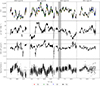 |
Fig. 4. Sgr A* ALMA light curves of the fractional polarization for the four spectral bands, the depolarization measure, the rotation measure, and the spectral index (from top to bottom) for all four days (from left to right, April 21, 22, 24, and 25). The gray-shaded band on April 24 marks the time range of the Chandra X-ray flare. |
Finally, the spectral index α is obtained by fitting the flux density variation across the ALMA frequency range using the model I = I0 ⋅ (ν/ν0)α, where I0 is the flux density at the reference frequency ν0. The resulting spectral index exhibits slight oscillations around zero, consistent with the findings from the 2017 light curves presented in Wielgus et al. (2022a). These variations are accompanied by high uncertainty, primarily driven by the short timescale variability of the spectral index and calibration effects. Factors such as the ALMA intra-site antenna configuration, or the calibrator targets and the minispiral model used in QA2 and intra-field calibration, contribute to uncertainties in the absolute flux density across SPWs.
The variability of the full-polarization Sgr A* light curves, characterized by the modulation index and other advanced time-series analysis tools, are explored in detail in Sect. 4.
3.2. Comparison to historical data
To investigate long-term trends in Sgr A*’s behavior, we analyze historical flux density and polarization data from 2005 to 2019, as compiled in Table 6 of Wielgus et al. (2022a). Figure 5 presents the flux density as a function of time, showing that the daily average values from 2018 fall within the range of previously reported measurements. The data also align with a broader trend of increasing average flux density from 2017 (Wielgus et al. 2022a) to 2019 (Murchikova & Witzel 2021).
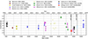 |
Fig. 5. Historical 230 GHz amplitude measurements of Sgr A* from 2005 to 2019 in Table 4 of Wielgus et al. (2022a) and average flux density and standard deviation from Table E.1. The 2017 and 2018 EHT observing campaigns are marked by black vertical lines. Standard deviations for both the 2017 and 2018 EHT observations are plotted, but are too small to be visible. |
An examination of the modulation indices further supports consistency with past observations (Fig. 6). Comparing our derived modulation indices with the damped random walk (DRW) model fitted to historical data by Wielgus et al. (2022a), we find that variability in 2018 was slightly lower than the expected value from the model. However, a direct comparison of the modulation indices from full-polarization ALMA light curves in the 2017 and 2018 campaigns reveals consistent values across both years, as well as notable stability throughout the entire experiment (Fig. 7).
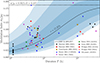 |
Fig. 6. Modulation index measured across various observations as a function of observational duration. Each data point from the 2018 ALMA dataset at B3 (227 GHz) is represented by hexagons, while other data points, as well as the fitted damped random walk (DRW) curve with shaded confidence intervals are derived from Wielgus et al. (2022a). |
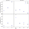 |
Fig. 7. Modulation indices σ/μ of the Stokes I (top) and polarized intensity (bottom) ALMA light curves, for the 2017 and 2018 observations at B1 (black dots) and B4 (blue diamonds), obtained from our analysis. |
The average linear polarization fraction across the four SPWs ranges from 3.8% to 5.8%, slightly lower than the 2017 ALMA values of 7.7%–8.5% reported in Wielgus et al. (2024). Nonetheless, these values remain broadly consistent with historical measurements spanning 3.6%–9.9% (Bower et al. 2003, 2005; Marrone et al. 2007; Bower et al. 2018). The average EVPA across spectral windows ranged from –70.30° to –117.97°. The spread in EVPA values seen in Fig. 3 reflects short-term variability in Sgr A*, while the broader range observed over nearly 20 years (Bower et al. 2003, 2005; Marrone et al. 2007; Bower et al. 2018; Wielgus et al. 2022b) suggests significant long-term evolution in the linear polarization.
For circular polarization, we observe daily averages ranging from –0.41% to –1.0% in 2018. The most negative values align with the 2017 ALMA results, which reported an average CP of –1.0% to –1.6% (Goddi et al. 2021; Wielgus et al. 2024), as well as with Bower et al. (2018), who found a mean CP of –1.1 ± 0.2% at 225 GHz in 2016. We note, however, that all of these circular polarization measurements should be regarded as tentative detections, as the measured levels fall below the official CP accuracy threshold guaranteed by the ALMA observatory.
The daily average RM in our 2018 data ranges from −5.32 × 10⁵ to −2.63 × 10⁵ rad m−2, comparable to 2017 ALMA results, which reported daily averages between −5.04 × 10⁵ and −3.19 × 10⁵ rad m−2 (Goddi et al. 2021; Wielgus et al. 2024). Our values are also consistent with past measurements over the last two decades from ALMA (Bower et al. 2018), SMA (Marrone et al. 2007), and BIMA (Bower et al. 2003, 2005). This agreement suggests a relatively stable long-term Faraday rotation, while also reflecting short-term variability in Sgr A*’s polarization properties.
4. Time-series analysis of the Sgr A* light curves
4.1. Cross-correlations between Spectral Windows
To compute the correlation of the Sgr A* light curves at different SPWs, we used the Locally Normalized Discrete Correlation Function (LNDCF; see Lehar et al. 1992). The LNDCF consists of binning pairs of flux density measurements (ai, bj) by a time difference (lag Δt), and then computing estimates of the correlation between the two signals using the formula
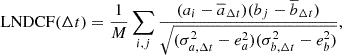 (4)
(4)
where M is the number of data pairs in the lag bin Δt, ea and eb represent the measurement errors of the data points of their respective signals, and the signal amplitudes and standard deviations (i.e.,  ,
,  , σa, Δt2, σb, Δt2) are computed for each lag using the flux densities contributing to the LNDCF. Here, we define LNDCF(0) = LNDCF0.
Given the abundance of light curves available (one for each parameter, day of observation of Sgr A* and spectral window), we first computed the LNDCF between SPWs. Strongly correlated signals between SPWs (i.e., LNDCF0 ≳ 0.95) suggest similarity in the information provided by the different spectral windows from a physical perspective. As illustrated in Fig. 8, a strong correlation exists between the different SPWs, particularly within the same spectral band, both for the total intensity and the polarized intensity. Consequently, focusing our study on one spectral window per band for the subsequent analysis is appropriate, a conclusion further supported by individual inspections of each spectral window.
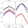 |
Fig. 8. LNDCF between SPWs B1–B2 (black dots), B1–B4 (red squares), and B3–B4 (blue diamonds), for total flux density (left) and polarized intensity (right), for April 24. |
Examining the LNDCF between SPWs across various spectral bands (B1–B4) at minute-scale time lags, as depicted in Fig. 9, reveals a clearer shift in the maximum of the LNDCF for polarized intensity on April 24, with a delay of −21 ± 13 seconds, i.e., with the light curve at B1 lagging behind that at B4. This delay, occurring on the day Chandra reported a flare, is consistent, although less pronounced than the delay of −45 ± 15 seconds reported in Wielgus et al. (2022b), Appendix G, observed on April 11, 2017, when a flare was also detected by Chandra. In contrast, the delays observed on other days remain consistent with zero: 7 ± 9 seconds on April 21, 6 ± 10 seconds on April 22, and −3 ± 11 seconds on April 25. No significant delay is observed for total intensity, remaining consistent with zero across all days.
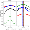 |
Fig. 9. LNDCF between ALMA SPWs B1-B4 for all four days, showing total flux density (left) and polarized intensity (right). The dotted lines indicate the delays between SPWs B1–B4 retrieved from the LNDCF. |
4.2. Structure function
The structure function (SF) of the polarized flux density serves as a powerful diagnostic of variability in the emission, revealing characteristic timescales and amplitudes that are sensitive to the turbulence within the accretion flow. In particular, short timescale variability is expected to originate from turbulent processes occurring close to the black hole. Moreover, GRMHD simulations predict that the variability power spectrum depends on the underlying magnetic field configuration, typically modeled as either a MAD or SANE accretion flow (e.g., Event Horizon Telescope Collaboration 2022c; Moscibrodzka 2024). As these models differ significantly in their magnetic flux distribution and turbulence levels, the results from the SF analysis provide insight into the plasma conditions near the event horizon.
To characterize the power spectrum and retrieve the characteristic variability timescales of our Sgr A* light curves, both in total flux density and polarization, we analyzed the behavior of the first-order SF (see Simonetti et al. 1985; Wielgus et al. 2022a). Given a time series {xi}=x1, x2, …, xn observed at times {ti}=t1, t2, …, tn, the SF at a time lag Δt is defined as the sum of all the pairs in the time series, NΔt, for which (tj − ti)≤Δt,
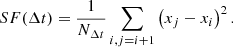 (5)
(5)
The analysis of the SF provides information on the temporal structure of our light curves. The SF of a signal affected by measurement and calibration errors, and random noise, such as the ones analyzed in this work, presents three types of slopes in the data (see Fig. 10):
-
At very short timescales, the slope of the SF is almost flat, and corresponds to the level of the noise, which dominates the amplitude of our signal. This SF plateau level is twice the variance of the noise in the data. The higher the noise, the higher the plateau, which could hide the signal properties.
-
A steep increase in the SF, as a result of the random noise becoming less dominant compared with the real signal in our data, indicating real variability in our data. The power spectral density (PSD) slope index αPSD can be calculated using the slope index αSF of this increase in the SF, which follows a power law, as αPSD = −(1 + αSF).
-
A plateau at long time lags, providing an estimate on the characteristic timescale of the light curves’ variability.
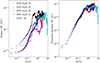 |
Fig. 10. SF plots of the Sgr A* 213.1 GHz light curves for total intensity (left) and polarized intensity (right), for April 21, 22, 24 and 25, and all combined (black dots, blue squares, red diamonds, magenta triangles, and cyan crosses, respectively). |
In Fig. 10 we observe that while the shapes of the total intensity SFs differ greatly across different days, both the shapes and timescales of the polarized intensity SFs are very consistent. Moreover, the SF for polarization is highly coherent, in contrast to the total flux density SF. This suggests that polarization arises from a coherent emission region, while total flux density comprises contributions from different, less coherent regions.
The results of the SF analysis, described in detail in Appendix F, are summarized in Table 1 (which also includes the results from the high-pass filter periodogram; see Appendix G). We present the results only for the SPWs B1 and B4, as they are representative of the two ALMA lower and upper spectral sidebands. Moreover, there are no significant differences in the SF between SPWs B1–B2 and B3–B4, as evidenced by the strong correlation between different SPWs shown in Fig. 8, so analyzing the timescales for all SPWs would yield similar results.
Results from the time-series analysis of the ALMA Sgr A* light curves in total flux density and polarized intensity.
Q − U loop speeds and fraction of scans that are clockwise.
To conclude the SF analysis, we applied the same procedure used to estimate the PSD and timescales from the SF of the 2018 light curves to the full-polarization light curves obtained from the ALMA April 2017 observations, presented in Fig. I.1. Figure 11 presents a comparison between the results of the SF analysis of the 2017 light curves (shown in Appendix I) and the 2018 light curves. We observe fluctuations in the timescales for total intensity, while the results for polarized intensity display a stable timescale across both years, around 0.5–0.6 hours. This consistency further supports the argument that Sgr A* polarization arises from a coherent emission region.
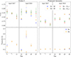 |
Fig. 11. PSD slope index (top) and timescales (bottom) estimated from the SF of the total intensity (left) and polarized intensity (right) 2017 and 2018 light curves, for the spectral bands B1 (blue dots) and B4 (orange squares). A second characteristic PSD and timescale, derived from the Stokes I SF, are marked with a cross (x). PSD values are computed from the SF slope as αPSD = −(1 + αSF) (blue dots and orange squares for the spectral bands B1 and B4, respectively), and from the HPF periodogram (red triangles and green diamonds for the spectral bands B1 and B4, respectively; see Appendix G). |
5. Discussion
5.1. Polarimetric loops
Coherent variation of the measured linear polarization, forming loops in the Q − U plane, can serve as a useful tool to constrain the models of the Sgr A* geometry, as discussed in Wielgus et al. (2022b). Such patterns may be associated with bubbles of strongly energized electrons forming as a consequence of a rapid release of magnetic energy into plasma, observed as a high-energy flare. Such bubbles (hotspots) could then transiently orbit the central black hole before being destroyed by instabilities, shearing in a differentially rotating flow, and/or radiatively cooling. Vos et al. (2022) and Vincent et al. (2024) provided detailed theoretical discussions on the formation of Q − U loops, similar to the observational signatures identified in the infrared observations of flaring Sgr A* (GRAVITY Collaboration 2018, 2023; Yfantis et al. 2024b). The millimeter wavelength polarimetric signatures associated with the 2017 April 11 X-ray flare were systematically studied and modeled by Yfantis et al. (2024a) and Levis et al. (2024), both concluding consistency with a clockwise hotspot motion in a compact orbit at a low inclination, as well as the dominance of a vertical magnetic field component. In Fig. 12, we present the polarimetric Q − U plane variation observed by ALMA in April 2018, including April 24, when Chandra reported an X-ray flare (Mossoux et al. 2020). Some more discussion about the flare is given in Sect. 5.2.
 |
Fig. 12. Sgr A* ALMA polarimetric loops observed in April 2018, for the spectral band B4, for all four days. The colors of the data points represent the time evolution of the Q − U behavior. |
By eye, the 2018 Q − U data do not readily exhibit coherent looping behavior that could be interpreted as orbital motion. This is in contrast to the 2017 April 11 flare, for which the loop is apparent; see Fig. 1 of Wielgus et al. (2022b). However, Ricarte et al. (2025) recently developed a method to determine Q − U rotation speeds and preferential handedness of the pattern using the differential geometry of planar curves. The method is capable of statistically characterizing the local curvature on the Q − U plane and infer the corresponding mean angular velocity, even in cases for which the coherent looping behavior is not visually apparent. In brief, smoothing splines are fit to each scan, and the signed Gaussian curvature is integrated over these light curves with respect to the arc length to obtain an average Q − U rotation rate and clockwise fraction. In this previous work, for the 2017 data of Wielgus et al. (2022b), Ricarte et al. (2025) calculated a pattern speed of ΩQU = −2.6 ± 0.6 deg tg−1, where tg = GMc−3 = 20 s, and that 65%±9% of the scans were curved in a clockwise orientation.
We repeated this analysis for the ALMA 2018 light curves presented in this paper, and the results are shown in tab:curvatures. We considered only the B4 light curves, as the EVPA evolution is almost identical across the four SPWs. This technique is not affected by an overall offset due to the RM. It may, however, be sensitive to the variable internal Faraday effects in Sgr A* (Wielgus et al. 2024). Systematic error bars were computed by surveying over spline fitting parameters as in Ricarte et al. (2025). We consistently recover clockwise motion on all days, similar to the 2017 data. Intriguingly, the most clockwise-biased day is the flaring day, 2018 April 24. Similarly, Ricarte et al. (2025) reported that the flaring period of 2017 April 11 is atypically biased towards clockwise as well. This suggests that Q − U loops may become more coherent during flares, possibly due to the emergence of a dominant polarized hotspot.
For the 2018 data, our all-day average Q − U rotation rate of −1.6 ± 0.9 deg tg−1 is consistent within 1σ with the 2017 measurement reported by Ricarte et al. (2025). This agreement suggests a relatively coherent clockwise accretion flow persisting over a timescale of 1.0 yr ≈ 1.6 × 10⁶ tg. Continued monitoring will be important to assess the long-term stability of this behavior.
One possible explanation for the observed differences between the coherent loopy pattern seen during the 2017 April 11 flare and the more disordered pattern observed on 2018 April 24 is that the 2018 X-ray flare did not actually originate in the immediate vicinity of the event horizon, where the millimeter synchrotron radiation is emitted. However, in Sect. 5.2 we discuss hints of causal relation between the high-energy flare and the millimeter ALMA light curves. Another possibility is the formation of a dominant single hotspot on 2017 April 11 and multiple simultaneous hotspots on 2018 April 24. While presence of several orbiting hotspots may scramble the detailed Q − U signatures, the overall clockwise rotation pattern could still be maintained, driven by components moving with a characteristic orbital velocity. Continuous monitoring of Sgr A* in X-ray and in millimeter is necessary to determine whether formation of coherent Q − U loops associated with high-energy flaring is common.
5.2. High-energy flare
On 2018 April 24 a high-energy flare from Sgr A* was detected by the Chandra X-ray Observatory. Unlike the X-ray flare observed on 2017 April 11 (Event Horizon Telescope Collaboration 2022b; Wielgus et al. 2022b), which occurred just before the start of the ALMA observations, the more powerful, double-peaked 2018 flare was captured during the ALMA coverage. A comparison between the Chandra and ALMA observations for the two events is shown in Fig. 13. While delays between high-energy and millimeter peaks are commonly observed (e.g., Yusef-Zadeh et al. 2008; Michail et al. 2024), the second peak of the 2018 flare appears to coincide with the maximum of the millimeter radio emission. This behavior is reminiscent of the IR/submillimeter flare reported by Fazio et al. (2018).
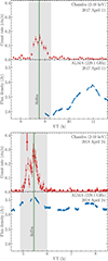 |
Fig. 13. Chandra counts (top) and Sgr A* total intensity ALMA light curves (bottom) for the flares observed in 2017 and 2018 during the EHT campaigns. The gray-shaded band marks the time range of the high-energy flare, with indicated maximum. |
Although the apparent alignment between the X-ray and millimeter light curves could occur by chance, given that the millimeter emission exhibits continuous red noise variability with local maxima typically occurring every few hours, there are reasons to suspect a physical connection. In particular, both magnetic reconnection events and millimeter-wavelength synchrotron emission in Sgr A* are expected to originate in the innermost regions of the accretion flow, near the event horizon. Assuming a causal link between the X-ray and millimeter peaks, the standard interpretation involving a transient, energized component that subsequently cools (producing delayed emission at lower frequencies) could not explain the observed simultaneity. An alternative explanation is that the X-ray and millimeter emissions are co-located and co-moving, and that the observed peak results from a Doppler boost associated with the motion of the emitting region. Such simultaneous emission across a broad energy range could arise if the emission region is optically thin and continuously energized, allowing for a mix of electron populations – some cooling while others are still being accelerated.
Further evidence supporting a causal link comes from the polarized light curves. On the flare day, an inter-band delay in the polarization amplitude |P| is detected, with B1 lagging behind B4 by 21 ± 13 s (see Fig. 9). This is comparable to the 45 ± 15 s lag reported during the 2017 flare (Wielgus et al. 2022b). In both the 2017 and 2018 data sets, delays in the other Stokes parameters, as well as |P| delays on non-flaring days, are consistent with zero. Finally, the millimeter light curves exhibit enhanced variability around the time of the flare (see Sect. 5.3), and the clockwise coherence of the Q–U polarization loop pattern is strongest on the flare day (Sect. 5.1). Taken together, these findings offer compelling evidence for a causal connection between the April 24 X-ray flare and its millimeter counterpart.
5.3. Comparison with GRMHD variability
In Event Horizon Telescope Collaboration (2022c) the variability of Sgr A*, constrained by ALMA observations (Wielgus et al. 2022a), was compared to predictions of general relativistic magnetohydrodynamic (GRMHD) simulations in the EHT simulation library (Event Horizon Telescope Collaboration 2022c; Dhruv et al. 2025b). The variability metric used was the M3 parameter, defined as the ratio of standard deviation to mean value (i.e., the modulation index) calculated over 3 hours long independent segments of total intensity light curves. The analysis revealed a systematic mismatch between most GRMHD models, particularly the strongly magnetized ones preferred by the static consistency metrics (Event Horizon Telescope Collaboration 2022c, 2024), and the observations. The numerical simulations appear to overproduce variability. Here, we extended the previous work by incorporating 2018 ALMA light curves presented in this paper. In total, we have five independent measurements of M3 from 2017 and nine from 2018, plotted in red in Fig. 14 (with the 2017 data in a darker share). A single outlier with M3 ≈ 0.1 corresponds to radio observations following an X-ray Chandra flare on 2017 April 11 (Event Horizon Telescope Collaboration 2022b; Wielgus et al. 2022b). Apart from this case, both 2017 and 2018 measurements indicate consistently low amount of variability; see also Fig. 7. The variability does not increase significantly on 2018 April 24, when another X-ray flare was detected by Chandra (Mossoux et al. 2020), although it is slightly elevated earlier on that day relative to later time, with M3 = (0.047, 0.029, 0.019) over three subsequent 3 h long observing periods (the X-ray flare occurred near the end of the first 3 h period).
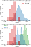 |
Fig. 14. Distribution of M3 in ALMA observations taken during the 2017 and 2018 EHT campaigns, compared to the distributions from different GRMHD models. The top panel shows the comparison with the EHT library of GRMHD models, while the bottom panel shows the comparison with the 1T and 2T GRMHD models from Salas et al. (2025). The dark red part of the observational histogram represents the 2017 ALMA data from Wielgus et al. (2022a), and the light red part corresponds to the 2018 results introduced in this paper. |
We compared the M3 values measured in the Stokes I observations with those derived from GRMHD simulations in the EHT library. We included 9720 synthetic light curves, each of a duration of 540 GMc−3 ≈ 3 h. The synthetic light curves were generated from 10 independent GRMHD simulations (strongly or weakly magnetized accretion state and 5 black hole spin values), each with 36 different radiative transfer choices for thermal relativistic distribution of energy of electrons (nine inclination angles times four values of the ion-to-electron temperature ratio parameter Rhigh). Additional details are given in Event Horizon Telescope Collaboration (2022c).
The mismatch between the observed variability and that predicted by the simulations persists, suggesting that standard fluid models may be inadequate for describing the properties of turbulent, collisionless astrophysical plasmas. The accretion flow surrounding Sgr A* is most likely collisionless (Mahadevan & Quataert 1997; Event Horizon Telescope Collaboration 2022c), where the electron-ion collision timescale is much longer than the accretion timescale. Under these conditions, the ions and electrons likely to maintain different temperatures (Shapiro et al. 1976; Rees et al. 1982).
Most GRMHD models consider a single-temperature ion (1T) plasma, where the electron density and temperature are not considered in the evolution equations (Gammie et al. 2003; Tchekhovskoy et al. 2011). In these 1T simulations, the ion-to-electron temperature ratio Ti/Te is set by the R(β) prescription, governed by the parameter Rhigh (Mościbrodzka et al. 2016), which constitutes one of the main uncertainties in EHT modeling. The discrepancy in 230 GHz variability may partially stem from not self-consistently modeling the evolution of Te when using the R(β) prescription. In reality, Te is determined by microphysical plasma processes and radiation interactions, rather than simply by Ti. A first-principles kinetic approach is required to completely model these collisionless effects (Parfrey et al. 2019; Crinquand et al. 2022; Galishnikova et al. 2023).
Nonetheless, it is possible to effectively model the electron thermodynamics with two-temperature (2T) treatments in GRMHD simulations by describing a gas consisting of ions and electrons that share the same dynamical equations but have independent thermodynamical evolution (e.g., Ressler et al. 2015; Sądowski et al. 2017; Chael et al. 2018). 2T treatments in strongly magnetized simulations more accurately predict 230 GHz variability in Sgr A* compared to 1T simulations; see Fig. 14. Moreover, including radiative synchrotron cooling of electrons in 2T treatments further decreases M3 relative to uncooled simulations (Salas et al. 2025). These results are consistent with theoretical expectations that the difference in adiabatic indices4 between relativistic electrons and non-relativistic ions effectively suppress fluctuations in the electron temperature (Gammie 2025; Salas et al. 2025). Moscibrodzka (2024) demonstrated that 2T strongly magnetized models exhibit less variability at 230 GHz compared to 1T models. They find that M3 increases with black hole spin but decreases slightly when non-thermal electron physics are included in the ray-tracing.
The collisionless nature of low-luminosity accretion flow such as in Sgr A* highlights the importance of non-ideal physics stemming from long mean free paths of particles. Dhruv et al. (2025a) consider one such weakly collisional model (Chandra et al. 2015), which includes viscosity and heat conduction. They find that incorporating these low-collisionality effects systematically lowers the 230 GHz variability in all MAD models. Additionally, Nathanail et al. (2025) explore how the inclusion of explicit resistivity reduces the variability of GRMHD simulations, potentially helping to reconcile the different accretion flow models.
Apart from the amount of variability, we are interested in its power distribution across frequencies, as discussed using SF in Sect. 4.2. As demonstrated by Wielgus et al. (2022a), GRMHD models generally indicate a steep power law of the short timescale variability αPSD between –2.5 and –2.9. This is steeper than the DRW process, characterized by αPSD = −2. The power law in the 2017 ALMA total intensity light curves was estimated by Wielgus et al. (2022a) to be αPSD ≈ −2.6, which broadly agrees with the predictions of numerical models. We see consistent estimates of αPSD in the 2018 data set, as presented in Fig. 11 and in Table 1. It is also worth noticing that we consistently see a sub-hour decorrelation timescale through the PSD and SF analysis, Table 1. While these findings seem to suggest that such an analysis is sensitive to dynamical timescales in the Sgr A* system, these conclusions must be carefully tested and verified, particularly since the ALMA light curves data can be fitted well with stochastic Gaussian process models of significantly longer correlation timescales (Wielgus et al. 2022a).
6. Conclusions
This work presents a comprehensive analysis of high-cadence, high signal-to-noise full-polarization light curves of Sgr A*, obtained with ALMA during the April 2018 EHT campaign. Notably, during the same week, the Chandra X-ray Observatory reported a flare on April 24 (between 4:53 and 6:00 UT), enabling a joint analysis of the millimeter and X-ray light curves on the day of the flare.
We first characterized the overall variability in total intensity, which remains low, with σ/μ < 10%, consistent with previous EHT campaigns and earlier observations. The estimated variability remains below the levels predicted by standard accretion flow models, though recent GRMHD simulations yield similarly reduced variability (Moscibrodzka 2024; Salas et al. 2025; Nathanail et al. 2025; Dhruv et al., in prep.). In contrast, the polarized intensity shows stronger variability, with σ/μ ∼ 30%.
To quantify the polarization variability, we employed advanced time-series analysis tools. Cross-correlations between the four spectral windows (B1–B4) reveal strong inter-band coherence, with LNDCF0 ≳ 0.95. On minute timescales, we detect no measurable delays between B1 and B4 for total intensity, consistent with optically thin synchrotron emission at 1.3 mm, an interpretation supported by the 2017 campaign as well. For the polarized intensity, delays are consistent with zero on most days, though with marginal positive shifts on April 21–22 and marginal negative ones on April 25. On April 24 – the day of the X-ray flare – we detect a statistically significant delay of 21 ± 13 s, with B1 lagging B4. A similar delay was reported for the 2017 flare event, further strengthening the association between polarization structure and high-energy activity.
The high quality of the ALMA light curves enabled variability analysis on short timescales. Both the SF and high-pass filter (HPF) periodogram analyses reveal red-noise behavior spanning timescales from minutes to hours. The derived power spectral densities are consistent across methods: −2.4 ± 0.3 for total flux density (matching the 2017 value) and −2.6 ± 0.1 for polarized intensity. Structure function analysis further reveals intra-day variability timescales of ∼20 minutes to 1.5 hours in total intensity, while the polarized intensity remains stable around ∼30 minutes – suggesting a more coherent emission region for the polarized component.
The April 24 X-ray flare offers a rare opportunity to probe the connection between X-ray and millimeter-wavelength emission. While previous flares (e.g., April 11, 2017) exhibited millimeter counterparts delayed by several hours, the 2018 event reveals near-simultaneous peaks in X-ray and millimeter emission, within a five-minute window. This is accompanied by a ∼20% increase in millimeter flux density. This simultaneity is further supported by an inter-band delay in polarized intensity (21 ± 13,s), an enhanced coherence in the Q–U polarization loops (clockwise direction), and an increased intra-day millimeter variability during the flare (with a subsequent decline thereafter). These findings challenge the standard scenario of delayed synchrotron emission from a cooling, expanding component. Instead, they support a scenario in which the emission region is optically thin and continuously energized, allowing both electron cooling and re-acceleration to occur concurrently.
A detailed analysis of the Q–U loop rotation rate reveals a persistent clockwise pattern, consistent with 2017 observations (Ricarte et al. 2025). This suggests a coherent structure in the underlying accretion flow on year-long timescales – corresponding to ∼1.6 × 10⁶ tg. This persistence provides a non-trivial constraint for GRMHD simulations and warrants comparison with wind-fed accretion flow models (e.g., Ressler et al. 2020). Continued monitoring of Sgr A* will be essential to assess the long-term stability of this signal.
Finally, similar to the essential role played by the 2017 ALMA light curve in constraining the temporal variability of Sgr A* and supporting the data calibration for horizon-scale imaging (Blackburn et al. 2019; Wielgus et al. 2022a; Event Horizon Telescope Collaboration 2022b), the characteristics of the 2018 ALMA light curve exert a similarly critical influence on the imaging based on the 2018 EHT observations (EHT Collaboration, in prep.). In addition, it provides complementary information on the source’s variability, contributing to a more comprehensive understanding of its temporal behavior.
Acknowledgments
The Event Horizon Telescope Collaboration thanks the following organizations and programs: the Academia Sinica; the Academy of Finland (projects 274477, 284495, 312496, 315721); the Agencia Nacional de Investigación y Desarrollo (ANID), Chile via NCN19_058 (TITANs), Fondecyt 1221421, BASAL FB210003; the Alexander von Humboldt Stiftung; an Alfred P. Sloan Research Fellowship; Allegro, the European ALMA Regional Centre node in the Netherlands, NOVA, and the astronomy institutes of the Universities of Amsterdam, Leiden, and Radboud; the ALMA North America Development Fund; the Black Hole Initiative (John Templeton Foundation grants 60477, 61497, 62286; Gordon and Betty Moore Foundation grant GBMF-8273); the Brinson Foundation; “la Caixa” Foundation (ID 100010434, LCF/BQ/DI22/11940027, LCF/BQ/DI22/11940030); the Canada Research Chairs program; Chandra grants DD7-18089X, TM6-17006X; the China Scholarship Council; the China Postdoctoral Science Foundation (2020M671266, 2022M712084); Conicyt Fondecyt Postdoctorado (3220195); Consejo Nacional de Humanidades, Ciencia y Tecnología (CONAHCYT, Mexico, projects U0004-246083, U0004-259839, F0003-272050, M0037-279006, F0003-281692, 104497, 275201, 263356, CBF2023-2024-1102, 257435); Colfuturo Scholarship; the Junta de Andalucía (P18-FR-1769), the Consejo Superior de Investigaciones Científicas (2019AEP112); the Delaney Family John A. Wheeler Chair at Perimeter Institute; DGAPA-UNAM (IN112820, IN108324); the Dutch Research Council (NWO) VICI award (639.043.513), grant OCENW.KLEIN.113, Dutch Black Hole Consortium (NWA 1292.19.202); Dutch Supercomputers Cartesius and Snellius (NWO 2021.013); the EACOA Fellowship (ASIAA, NAOJ, CAS, KASI); the ERC Synergy Grants “BlackHoleCam” (610058), “BlackHolistic” (10107164); EU Horizon 2020 grants RadioNet (730562), M2FINDERS (101018682), FunFiCO (777740); ERC Advanced Grant “JETSET” (884631); EU Horizon Europe SE programme NewFunFiCO (10108625); Horizon ERC 2021 programme (101040021); FAPESP (2021/01183-8); Fonds de Recherche du Québec – Nature et Technologies (FRQNT); Fondo CAS-ANID CAS220010; Gordon and Betty Moore Foundation (GBMF-3561, GBMF-5278, GBMF-10423); the Institute for Advanced Study; the ICSC – Centro Nazionale di Ricerca in HPC, Big Data and Quantum Computing (NextGenerationEU); INFN Napoli TEONGRAV; the International Max Planck Research School for Astronomy and Astrophysics at Bonn and Cologne; EU NextGenerationEU RRF M4C2 1.1 project 2022YAPMJH; DFG research grant “Jet physics on horizon scales and beyond” (443220636); Joint Columbia/Flatiron Postdoctoral Fellowship (Simons Foundation); the Japan MEXT (JPMXP1020200109); JSPS Fellowship (JP17J08829); Joint Institute for Computational Fundamental Science, Japan; CAS Frontier Sciences Program (QYZDJ-SSW-SLH057, QYZDJSSW-SYS008, ZDBS-LY-SLH011); Leverhulme Trust Early Career Fellowship; the Max-Planck-Gesellschaft (MPG); the Max Planck Partner Group of MPG and CAS; MEXT/JSPS KAKENHI (18KK0090, JP21H01137, JP18H03721, JP18K13594, 18K03709, JP19K14761, 18H01245, 25120007, 19H01943, 21H01137, 21H04488, 22H00157, 23K03453); the Generalitat Valenciana GenT Project CIDEGENT/2018/021 and grant ASFAE/2022/018; MICINN Projects PID2019-108995GB-C22, PID2022-140888NB-C22; the Astrophysics and High Energy Physics programme by MCIN, with funding from NextGenerationEU (PRTR-C17I1). MIT International Science and Technology Initiatives (MISTI); the Ministry of Science and Technology (MOST) of Taiwan (various grants 103–110 listed); NSTC of Taiwan (111-2124-M-001-005, 112-2124-M-001-014, 112-2112-M-003-010-MY3); Taiwan MoE Yushan Young Scholar Program; National Center for Theoretical Sciences of Taiwan; NASA grants 80NSSC23K1508, 80NSSC20K0527, 80NSSC20K0645; NASA Hubble Fellowship Program (Einstein Fellowship; grants HST-HF2-51431.001-A, HST-HF2-51482.001-A, HST-HF2-51539.001-A, HST-HF2-51552.001A); NINS of Japan; National Key R&D Program of China (2016YFA0400704, 2017YFA0402703, 2016YFA0400702); NSTC (111-2112-M-001-041, 111-2124-M-001-005, 112-2124-M-001-014); the US NSF (AST-0905844, AST-0922984, AST-1126433, OIA-1126433, AST-1140030, DGE-1144085, AST-1207704, AST-1207730, AST-1207752, MRI-1228509, OPP-1248097, AST-1310896, AST-1440254, AST-1555365, AST-1614868, AST-1615796, AST-1715061, AST-1716327, AST-1726637, OISE-1743747, AST-1743747, AST-1816420, AST-1935980, AST-1952099, AST-2034306, AST-2205908, AST-2307887); NSF Astronomy and Astrophysics Postdoctoral Fellowship (AST-1903847); NSERC (Canada); NRF Korea (grants NRF-2015H1D3A1066561, RS-2024-00407499, 2019R1F1A1059721, 2021R1A6A3A01086420, 2022R1C1C1005255, 2022R1F1A1075115); NOVA Virtual Institute of Accretion fellowships; NOIRLab (AURA/NSF); Onsala Space Observatory (VR grant 2017-00648); Perimeter Institute (Government of Canada and Province of Ontario); Portuguese FCT (CEEC 5th edition, UIDB/04106/2020, UIDP/04106/2020, PTDC/FIS-AST/3041/2020, CERN/FIS-PAR/0024/2021, 2022.04560.PTDC); Princeton Gravity Initiative; Ministerio de Ciencia e Innovación, Spain (PGC2018-098915-B-C21, AYA2016-80889-P, PID2019-108995GB-C21, PID2020-117404GB-C21, RYC2023-042988-I); University of Pretoria and SuperMicro SEEDING GRANT 2020; Shanghai Municipality grant 22JC1410600; Shanghai CAS Pilot Program JCYJ-SHFY-2021-013; Spanish MCIN/AEI grant CEX2021-001131-S; the Spinoza Prize SPI 78-409; South African Research Chairs Initiative through SARAO (NRF grant 77948); Swedish Research Council (VR); the Taplin Fellowship; the Toray Science Foundation; UK STFC (ST/X508329/1); US DOE via LANL (contract 89233218CNA000001); YCAA Prize Postdoctoral Fellowship; NRF Korea/MSIT grant RS-2024-00449206; CAPES Brazil PROEX 88887.845378/2023-00; Millenium Nucleus NCN23_002 (TITANs); Comité Mixto ESO-Chile. This research has made use of NASA’s Astrophysics Data System. We gratefully acknowledge the support provided by the extended staff of the ALMA, from the inception of the ALMA Phasing Project through the observational campaigns of 2017 and 2018. This work has been supported by the grant PRE2020-092200 funded by MCIN/AEI/10.13039/501100011033 and by ESF invest in your future. The Submillimeter Array is a joint project between the Smithsonian Astrophysical Observatory and the Academia Sinica Institute of Astronomy and Astrophysics and is funded by the Smithsonian Institution and the Academia Sinica. We recognize that Maunakea, location of the SMA, is a culturally important site for the indigenous Hawaiian people; we are privileged to study the cosmos from its summit. This paper makes use of the following ALMA data: 2017.1.00797.V ALMA is a partnership of ESO (representing its member states), NSF (USA) and NINS (Japan), together with NRC (Canada), MOST and ASIAA (Taiwan), and KASI (Republic of Korea), in cooperation with the Republic of Chile. The Joint ALMA Observatory is operated by ESO, AUI/NRAO and NAOJ. We thank Frederic Vincent for his help.
References
- Albentosa-Ruiz, E., & Marchili, N. 2024, PASP, 136, 114502 [Google Scholar]
- Aschenbach, B., Grosso, N., Porquet, D., & Predehl, P. 2004, A&A, 417, 71 [NASA ADS] [CrossRef] [EDP Sciences] [Google Scholar]
- Balick, B., & Brown, R. L. 1974, ApJ, 194, 265 [NASA ADS] [CrossRef] [Google Scholar]
- Blackburn, L., Chan, C.-K., Crew, G. B., et al. 2019, ApJ, 882, 23 [Google Scholar]
- Bower, G. C., Wright, M. C. H., Falcke, H., & Backer, D. C. 2003, ApJ, 588, 331 [Google Scholar]
- Bower, G. C., Falcke, H., Wright, M. C., & Backer, D. C. 2005, ApJ, 618, L29 [Google Scholar]
- Bower, G. C., Markoff, S., Dexter, J., et al. 2015, ApJ, 802, 69 [Google Scholar]
- Bower, G. C., Broderick, A., Dexter, J., et al. 2018, ApJ, 868, 101 [NASA ADS] [CrossRef] [Google Scholar]
- Boyce, H., Haggard, D., Witzel, G., et al. 2019, ApJ, 871, 161 [NASA ADS] [CrossRef] [Google Scholar]
- Brentjens, M. A., & de Bruyn, A. G. 2005, A&A, 441, 1217 [NASA ADS] [CrossRef] [EDP Sciences] [Google Scholar]
- Brown, R. L., & Lo, K. Y. 1982, ApJ, 253, 108 [Google Scholar]
- Capellupo, D. M., Haggard, D., Choux, N., et al. 2017, ApJ, 845, 35 [Google Scholar]
- Chael, A., Rowan, M., Narayan, R., Johnson, M., & Sironi, L. 2018, MNRAS, 478, 5209 [NASA ADS] [CrossRef] [Google Scholar]
- Chandra, M., Gammie, C. F., Foucart, F., & Quataert, E. 2015, ApJ, 810, 162 [NASA ADS] [CrossRef] [Google Scholar]
- Crew, G. B., Goddi, C., Matthews, L. D., et al. 2023, PASP, 135, 025002 [NASA ADS] [CrossRef] [Google Scholar]
- Crinquand, B., Cerutti, B., Dubus, G., Parfrey, K., & Philippov, A. 2022, Phys. Rev. Lett., 129, 205101 [NASA ADS] [CrossRef] [Google Scholar]
- Dexter, J., Tchekhovskoy, A., Jiménez-Rosales, A., et al. 2020, MNRAS, 497, 4999 [Google Scholar]
- Dhruv, V., Prather, B., Chandra, M., Joshi, A. V., & Gammie, C. F. 2025a, ApJ, 993, L33 [Google Scholar]
- Dhruv, V., Prather, B., Wong, G. N., & Gammie, C. F. 2025b, ApJS, 277, 16 [Google Scholar]
- Do, T., Hees, A., Ghez, A., et al. 2019, Science, 365, 664 [Google Scholar]
- Eckart, A., Baganoff, F. K., Morris, M., et al. 2004, A&A, 427, 1 [NASA ADS] [CrossRef] [EDP Sciences] [Google Scholar]
- Eckart, A., Schödel, R., Meyer, L., et al. 2006, A&A, 455, 1 [NASA ADS] [CrossRef] [EDP Sciences] [Google Scholar]
- Eckart, A., García-Marín, M., Vogel, S. N., et al. 2012, A&A, 537, A52 [NASA ADS] [CrossRef] [EDP Sciences] [Google Scholar]
- Event Horizon Telescope Collaboration (Akiyama, K., et al.) 2022a, ApJ, 930, L12 [NASA ADS] [CrossRef] [Google Scholar]
- Event Horizon Telescope Collaboration (Akiyama, K., et al.) 2022b, ApJ, 930, L13 [NASA ADS] [CrossRef] [Google Scholar]
- Event Horizon Telescope Collaboration (Akiyama, K., et al.) 2022c, ApJ, 930, L16 [NASA ADS] [CrossRef] [Google Scholar]
- Event Horizon Telescope Collaboration (Akiyama, K., et al.) 2024, ApJ, 964, L26 [CrossRef] [Google Scholar]
- Fazio, G. G., Hora, J. L., Witzel, G., et al. 2018, ApJ, 864, 58 [NASA ADS] [CrossRef] [Google Scholar]
- Galishnikova, A., Philippov, A., Quataert, E., et al. 2023, Phys. Rev. Lett., 130, 115201 [NASA ADS] [CrossRef] [Google Scholar]
- Gammie, C. F. 2025, ApJ, 980, 193 [Google Scholar]
- Gammie, C. F., McKinney, J. C., & Tóth, G. 2003, ApJ, 589, 444 [Google Scholar]
- Genzel, R., Schödel, R., Ott, T., et al. 2003, Nature, 425, 934 [NASA ADS] [CrossRef] [Google Scholar]
- Goddi, C., Martí-Vidal, I., Messias, H., et al. 2019, PASP, 131, 075003 [Google Scholar]
- Goddi, C., Martí-Vidal, I., Messias, H., et al. 2021, ApJ, 910, L14 [NASA ADS] [CrossRef] [Google Scholar]
- Goddi, C., Carlos, D. F., Crew, G. B., et al. 2025, A&A, 699, A265 [NASA ADS] [CrossRef] [EDP Sciences] [Google Scholar]
- GRAVITY Collaboration (Abuter, R., et al.) 2018, A&A, 618, L10 [NASA ADS] [CrossRef] [EDP Sciences] [Google Scholar]
- GRAVITY Collaboration (Jiménez-Rosales, A., et al.) 2020, A&A, 643, A56 [CrossRef] [EDP Sciences] [Google Scholar]
- GRAVITY Collaboration (Abuter, R., et al.) 2022, A&A, 657, L12 [NASA ADS] [CrossRef] [Google Scholar]
- GRAVITY Collaboration (Abuter, R., et al.) 2023, A&A, 677, L10 [NASA ADS] [CrossRef] [EDP Sciences] [Google Scholar]
- Heywood, I., Rammala, I., Camilo, F., et al. 2022, ApJ, 925, 165 [NASA ADS] [CrossRef] [Google Scholar]
- Iwata, Y., Oka, T., Tsuboi, M., Miyoshi, M., & Takekawa, S. 2020, ApJ, 892, L30 [NASA ADS] [CrossRef] [Google Scholar]
- Johnson, M. D., Fish, V. L., Doeleman, S. S., et al. 2015, Science, 350, 1242 [Google Scholar]
- Joshi, A. V., Prather, B. S., Chan, C.-K., Wielgus, M., & Gammie, C. F. 2024, ApJ, 972, 135 [Google Scholar]
- Lehar, J., Hewitt, J. N., Roberts, D. H., & Burke, B. F. 1992, ApJ, 384, 453 [NASA ADS] [CrossRef] [Google Scholar]
- Levis, A., Chael, A. A., Bouman, K. L., Wielgus, M., & Srinivasan, P. P. 2024, Nat. Astron., 8, 765 [NASA ADS] [CrossRef] [Google Scholar]
- Macquart, J.-P., Bower, G. C., Wright, M. C. H., Backer, D. C., & Falcke, H. 2006, ApJ, 646, L111 [NASA ADS] [CrossRef] [Google Scholar]
- Mahadevan, R., & Quataert, E. 1997, ApJ, 490, 605 [Google Scholar]
- Marrone, D. P., Moran, J. M., Zhao, J.-H., & Rao, R. 2006, ApJ, 640, 308 [NASA ADS] [CrossRef] [Google Scholar]
- Marrone, D. P., Moran, J. M., Zhao, J.-H., & Rao, R. 2007, ApJ, 654, L57 [NASA ADS] [CrossRef] [Google Scholar]
- Marrone, D. P., Baganoff, F. K., Morris, M. R., et al. 2008, ApJ, 682, 373 [Google Scholar]
- Martí-Vidal, I., Vlemmings, W. H. T., Muller, S., & Casey, S. 2014, A&A, 563, A136 [Google Scholar]
- Martí-Vidal, I., Roy, A., Conway, J., & Zensus, A. J. 2016, A&A, 587, A143 [NASA ADS] [CrossRef] [EDP Sciences] [Google Scholar]
- Matthews, L. D., Crew, G. B., Doeleman, S. S., et al. 2018, PASP, 130, 015002 [Google Scholar]
- Michail, J. M., Yusef-Zadeh, F., Wardle, M., et al. 2024, ApJ, 971, 52 [Google Scholar]
- Moscibrodzka, M. 2024, arXiv e-prints [arXiv:2412.06492] [Google Scholar]
- Mościbrodzka, M., Falcke, H., & Shiokawa, H. 2016, A&A, 586, A38 [Google Scholar]
- Mossoux, E., Finociety, B., Beckers, J. M., & Vincent, F. H. 2020, A&A, 636, A25 [NASA ADS] [CrossRef] [EDP Sciences] [Google Scholar]
- Murchikova, L., & Witzel, G. 2021, ApJ, 920, L7 [NASA ADS] [CrossRef] [Google Scholar]
- Mus, A., Martí-Vidal, I., Wielgus, M., & Stroud, G. 2022, A&A, 666, A39 [NASA ADS] [CrossRef] [EDP Sciences] [Google Scholar]
- Nathanail, A., Mizuno, Y., Contopoulos, I., et al. 2025, A&A, 693, A56 [NASA ADS] [CrossRef] [EDP Sciences] [Google Scholar]
- Parfrey, K., Philippov, A., & Cerutti, B. 2019, Phys. Rev. Lett., 122, 035101 [Google Scholar]
- Porth, O., Mizuno, Y., Younsi, Z., & Fromm, C. M. 2021, MNRAS, 502, 2023 [NASA ADS] [CrossRef] [Google Scholar]
- Quataert, E., & Gruzinov, A. 2000, ApJ, 545, 842 [NASA ADS] [CrossRef] [Google Scholar]
- Rees, M. J., Begelman, M. C., Blandford, R. D., & Phinney, E. S. 1982, Nature, 295, 17 [CrossRef] [Google Scholar]
- Remijan, A., Biggs, A., Cortes, P. A., et al. 2019, https://doi.org/10.5281/zenodo.4511522 [Google Scholar]
- Ressler, S. M., Tchekhovskoy, A., Quataert, E., Chandra, M., & Gammie, C. F. 2015, MNRAS, 454, 1848 [Google Scholar]
- Ressler, S. M., White, C. J., Quataert, E., & Stone, J. M. 2020, ApJ, 896, L6 [NASA ADS] [CrossRef] [Google Scholar]
- Ricarte, A., Conroy, N. S., Wielgus, M., et al. 2025, ApJ, 987, 152 [Google Scholar]
- Ripperda, B., Liska, M., Chatterjee, K., et al. 2022, ApJ, 924, L32 [NASA ADS] [CrossRef] [Google Scholar]
- Sądowski, A., Wielgus, M., Narayan, R., et al. 2017, MNRAS, 466, 705 [NASA ADS] [CrossRef] [Google Scholar]
- Salas, L. D. S., Liska, M. T. P., Markoff, S. B., et al. 2025, MNRAS, 538, 698 [Google Scholar]
- Scargle, J. D. 1982, ApJ, 263, 835 [Google Scholar]
- Shapiro, S. L., Lightman, A. P., & Eardley, D. M. 1976, ApJ, 204, 187 [NASA ADS] [CrossRef] [Google Scholar]
- Shcherbakov, R. V., Penna, R. F., & McKinney, J. C. 2012, ApJ, 755, 133 [NASA ADS] [CrossRef] [Google Scholar]
- Simonetti, J. H., Cordes, J. M., & Heeschen, D. S. 1985, ApJ, 296, 46 [NASA ADS] [CrossRef] [Google Scholar]
- Smirnov, O. M. 2011, A&A, 527, A106 [NASA ADS] [CrossRef] [EDP Sciences] [Google Scholar]
- Sokoloff, D. D., Bykov, A. A., Shukurov, A., et al. 1998, MNRAS, 299, 189 [Google Scholar]
- Tchekhovskoy, A., Narayan, R., & McKinney, J. C. 2011, MNRAS, 418, L79 [NASA ADS] [CrossRef] [Google Scholar]
- The CASA Team, Bean, B., Bhatnagar, S., et al. 2022, PASP, 134, 114501 [NASA ADS] [CrossRef] [Google Scholar]
- Vincent, F. H., Wielgus, M., Aimar, N., Paumard, T., & Perrin, G. 2024, A&A, 684, A194 [NASA ADS] [CrossRef] [EDP Sciences] [Google Scholar]
- Vos, J., Mościbrodzka, M. A., & Wielgus, M. 2022, A&A, 668, A185 [NASA ADS] [CrossRef] [EDP Sciences] [Google Scholar]
- Wielgus, M., Marchili, N., Martí-Vidal, I., et al. 2022a, ApJ, 930, L19 [NASA ADS] [CrossRef] [Google Scholar]
- Wielgus, M., Moscibrodzka, M., Vos, J., et al. 2022b, A&A, 665, L6 [NASA ADS] [CrossRef] [EDP Sciences] [Google Scholar]
- Wielgus, M., Issaoun, S., Martí-Vidal, I., et al. 2024, A&A, 682, A97 [NASA ADS] [CrossRef] [EDP Sciences] [Google Scholar]
- Witzel, G., Martinez, G., Willner, S. P., et al. 2021, ApJ, 917, 73 [NASA ADS] [CrossRef] [Google Scholar]
- Yfantis, A. I., Mościbrodzka, M. A., Wielgus, M., Vos, J. T., & Jimenez-Rosales, A. 2024a, A&A, 685, A142 [NASA ADS] [CrossRef] [EDP Sciences] [Google Scholar]
- Yfantis, A. I., Wielgus, M., & Mościbrodzka, M. 2024b, A&A, 691, A327 [NASA ADS] [CrossRef] [EDP Sciences] [Google Scholar]
- Yuan, F., & Narayan, R. 2014, ARA&A, 52, 529 [NASA ADS] [CrossRef] [Google Scholar]
- Yuan, F., Quataert, E., & Narayan, R. 2003, ApJ, 598, 301 [Google Scholar]
- Yusef-Zadeh, F., Wardle, M., Heinke, C., et al. 2008, ApJ, 682, 361 [NASA ADS] [CrossRef] [Google Scholar]
This algorithm is incorporated into a CASA script and is described in detail in the EHT Memo 2025-TDWG-01. The full pipeline is available for download on GitHub: https://github.com/ealruiz/calminispiral.
The model for Stokes Q, U, V assumes a centered point source (i.e., Vmod = S, where S is the flux density of the core Stokes parameter), as the minispiral is unpolarized at millimeter wavelengths (see Goddi et al. 2021).
We have also reprocessed the 2017 light curves using the same intra-field calibration pipeline applied to the 2018 data; the results are shown in Appendix I.
The adiabatic index γ characterizes the fluid response to compression, relating gas pressure pg and density ρ via pg ∝ ργ.
ALMA Memo #594
The HPF periodogram tool (DOI: 10.5281/zenodo.13917829) is available for download on GitHub: https://github.com/ealruiz/HPF_Periodogram.
Appendix A: Absorption line at 227 GHz
Figure A.1 shows the spectrum of Sgr A* in the B3 spectral window on April 22, revealing clear absorption features in channels 17–33 and 56–112. These absorption features are consistently observed across all days of the campaign. Foreground absorption toward Sgr A* at 226.91 GHz was previously reported in the ALMA 2017 data by Goddi et al. (2021). This absorption causes a flux suppression of approximately 4% in the B3 spectral window. To ensure consistency across the Sgr A* light curves from all spectral windows, we flagged the frequency channels affected by absorption prior to further analysis.
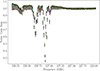 |
Fig. A.1. Bandpass of Sgr A* for the April 22 observations indicating the channels impacted by absorption at B3. The bandpass remains virtually unchanged across all days. |
Appendix B: Light curves of EHT targets
Figure B.1 shows the visibility amplitudes per integration time for each of the EHT targets observed alongside Sgr A*, on April 21, 22, 24, and 25. We display both the sum and difference of the parallel-hand correlations (XX and YY) and the cross-hand correlations (XY and YX), which correspond to the Stokes I, Q, U, and V light curves, respectively, according to the Radio Interferometer Measurement Equation formalism (Smirnov 2011). The visibility amplitude light curves confirm that, unlike Sgr A*, the other AGN targets exhibit stable flux densities throughout each night of observation. This stability is consistent with the modulation indices, at least an order of magnitude lower than those of Sgr A*, indicating that Sgr A*’s variability is intrinsic.
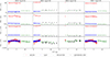 |
Fig. B.1. Reconstructed visibility-amplitude light curves for the EHT targets obtained with ALMA during the 2018 EHT VLBI campaign: 3C 279 (red circles), M87 (blue triangles), NRAO 530 (green diamonds), and QSO B1921-293 (black squares). |
Appendix C: Manual reduction of ALMA data
We employed a second independent method to derive the ALMA light curves. This method utilizes the SEFD-based data reduction process of "ALMA A2" described in Wielgus et al. (2022a) to produce calibrated data by correcting for atmospheric water vapor and antenna system temperature effects before performing a bandpass, flux density, and polarization calibration. Unlike ALMA A2, where visibilities on short baselines are flagged, this method (similar to that described in Sect. 2.2) accounts for the contributions of the minispiral to the observed variability and flux density, correcting for these effects.
Visibilities representing the point source were defined as those at a uv-distance greater than 50 m, while those at less than 50 m describe the minispiral plus time-variable point source. We used 50 meters rather than 50 kλ as a cutoff to ensure independence from the central wavelength of the spectral windows. Figure C.1 shows that most of the extended structure flux is seen on baselines shorter than 50 m, with the data at longer baselines predominantly corresponding to an unresolved point source as the angular resolution increases.
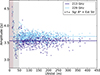 |
Fig. C.1. Snapshot of the calibrated data for Sgr A* at 7:23 UTC on April 25 from the SEFD-based data reduction. The colored circles represent the combined visibilities of the minispiral and Sgr A*. The solid colored lines are the mean flux density in each spectral window. The gray-shaded area represents the range of visibilities we consider for the minispiral (0-50 m). The red-shaded area represents the flagging cutoff for the extended structure used by SMA (0-30 kλ). |
As the first step of the analysis, phase self-calibration was performed on all data using the extended baselines (> 50 m) to remove residual phase errors, correcting each antenna to produce updated visibilities that describe a central point source.
Next, a central point source was fitted to all data for all baselines using the software package UVMULTIFIT (Martí-Vidal et al. 2014). The residual of this fit is the minispiral, which was then used for amplitude self calibration within each observing block of Sgr A* between calibrators.
Due to a lack of sufficient data at short baselines (< 50 m), some antennas were absent from the gain amplitude table generated from the minispiral. The gain amplitude from the minispiral self-calibration was applied to both the full (combined Sgr A* point source and minispiral) data and the minispiral-only data. The minispiral-only data was then subtracted from the full data, leaving behind a central point source.
This point-source-only data was subsequently used for amplitude self-calibration of the antennas that did not receive amplitude gains from the minispiral self-calibration. Finally, a last amplitude self-calibration was performed using all baselines. The resulting visibilities were used to calculate the total intensity of Sgr A*, which was then averaged for all baselines. Finally, the total intensity was plotted as a function of time to create the light curve.
Appendix D: SMA observations and data processing
SMA observed Sgr A* for roughly four hours (between 10 and 15 UT) in full-polarization mode, starting as the source was setting in Chile and rising in Hawaii. During these observations, SMA had either six or seven antennas on sky, with an integration time of 9.8 s and a total spectral bandwidth of 16 GHz (8 GHz per sideband, covering 208.1–216.1 and 224.1–232.1 GHz in the lower and upper sidebands, respectively). The array was configured in its extended mode, with typical baseline lengths ranging from 50 to 200 m.
SMA data were initially processed through the COMPASS pipeline (Keating et al., in prep.), which performs flagging and calibration. After applying bandpass corrections, the data were spectrally averaged by a factor of 128, yielding a final spectral resolution of 17.825 MHz. Bandpass solutions were obtained using 3C 279, while flux calibration was derived using Callisto and the Butler-JPL-Horizons 2012 models.5 Amplitude gains were solved using NRAO 530 and J1924–2914 (the latter observed during two tracks) and applied on an elevation-based basis, with typical amplitude corrections of order 5–10% below 25° in elevation. Due to strong line absorption features, spectral channels between 226.6 and 227.0 GHz were flagged (see Appendix A).
After applying the calibration gain solutions, self-calibration gains were derived under the assumption of a point-source model for Sgr A*, solving for a 10 s interval. Once self-calibration gains were applied, the SMA light curve was generated using a naturally weighted average of all visibilities for each time interval and spectral window. A final round of flagging was performed, removing data points with significant window-to-window or interval-to-interval variations. Finally, the data were averaged over seven integration intervals (equivalent to 70 s) to improve the signal-to-noise ratio.
Figure D.1 presents the QA2 ALMA and SMA light curves for each day across the four available bands. Visually, the two datasets exhibit similar structures during overlapping periods and display flux densities consistent within our estimated flux scale uncertainty of ⪅10%. To quantitatively assess the agreement between the SMA and ALMA light curves, we applied the Locally Normalized Discrete Correlation Function (LNDCF; Lehar et al. 1992), as detailed in Sect. 4.1. We analyzed the correlation during overlapping time intervals, matching spectral windows between the two datasets. The cross-correlation values are strong, reaching approximately 0.8±0.1 on April 22 and April 24, and 0.7±0.1 on April 25. On April 21, the LNDCF is slightly lower, around 0.6±0.1. The reduced correlation on April 21 and 25 is likely due to the lower elevation of Sgr A* during ALMA observations coinciding with SMA coverage, leading to lower observed flux densities and increased noise in the light curves. Given this overall consistency, also in agreement with the findings of Wielgus et al. (2022a), we based the subsequent variability analysis on ALMA data alone.
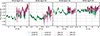 |
Fig. D.1. Sgr A* light curves for ALMA and SMA at all four available bands. |
Appendix E: Characteristics of the 2018 ALMA light curves
Table E.1 summarizes the main variability characteristics of the full-polarization Sgr A* 2018 ALMA light curves presented in this work and plotted in Figs. 3 and 4.
ALMA Sgr A* light curves, in total flux density, polarized intensity, and Stokes V, presented in this paper.
Appendix F: Details of the structure function analysis
Section 4.2 presents the main results of the SF analysis of the Sgr A* 2018 ALMA light curves. In this appendix we examine in greater detail the behavior of the SF and describe the methodology employed to estimate PSD slopes and variability timescales.
In Fig. 10 the SF of total intensity for April 21 presents a steep increase at a shorter time lag than the other days, and a noticeable dip at long timescales, where a clear plateau is usually expected. Inspection of the light curves presented in Fig. 3 reveals that this feature arises from data sampling, particularly the sudden increase in flux density around 3.5 hours, where there is a gap in observation that does not capture the complete increase in flux density (i.e., it is a consequence of an extreme event in our data). The sampling effect on the SF, together with the limited duration of our light curves, also explains the oscillations of the plateau at long timescales.
To compute the timescales of the light curves, we first fitted a slope to the values of the SF at the steep increase time lags, and retrieved the plateau level (as illustrated in some examples in Fig. F.1). The intersection of the slope and plateau level gives us the timescales. Since the SF presents a clear plateau at long timescales (despite some oscillations caused by the sampling), these timescales are characteristic of our light curves.
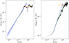 |
Fig. F.1. Sample of SF fitted to retrieve the slope (blue line, with an area corresponding to the 3σ level), the plateau level (orange line) and the timescales (red point, marking the intersection of the slope and the plateau). Left: SF of the April 21 Stokes I denoised light curve. Right: SF of the April 22 Stokes I light curve; we note two distinct slopes, fitted independently (the second slope corresponds to the green line). |
The timescales of the Sgr A* total flux density (except for April 22) were computed after denoising the light curve. This process involved binning the data using a window approximately two times the observational cadence and fitting a spline to the resulting light curve. This effectively reduced noise while preserving the main features of the signal, mitigating noise that could affect the SF slope estimates for the total flux density. In the SF of the April 22 total flux density, two distinct slopes are observed, revealing two characteristic timescales (see Fig. F.1).
Denoising was not applied to the April 22 data because, unlike the other days, the shape of the SF enables a good estimate of the two slopes after removing the time lags affected by white noise in the signal (as shown in Fig. F.1). Moreover, denoising would affect the estimate of the first slope, since short time lags are more affected by white noise in our signals, and the presence of two timescales restricts the sampling used to estimate the first slope, making this estimate more sensitive to denoising.
Appendix G: Periodogram results
To characterize the variability of the full-polarization 2018 Sgr A* light curves, we employed the SF in Sect. 4, which yields both the characteristic timescale and the Power Spectral Density (PSD) slope of the light curves.
An alternative method for characterizing the PSD slope of a signal is the Lomb-Scargle periodogram, commonly used in astronomy to account for non-uniform sampling and gaps in time-series data, such as those present in our light curves (see Fig. 3). The Lomb-Scargle periodogram at a given frequency ω is defined following the formulation stated in Scargle (1982), as
![Mathematical equation: $$ \begin{aligned} P_X (\omega ) = \frac{1}{2} \Bigg \{ \frac{ \left[ \sum _j X_j \cos \omega (t_j - \tau ) \right]^2 }{ \sum _j X_j \cos ^2 \omega (t_j - \tau ) } + \frac{ \left[ \sum _j X_j \sin \omega (t_j - \tau ) \right]^2 }{ \sum _j X_j \sin ^2 \omega (t_j - \tau ) } \Bigg \}, \end{aligned} $$](/articles/aa/full_html/2026/04/aa56759-25/aa56759-25-eq32.gif)
where X is the physical signal measured at a set of times tj, resulting in time-series data {Xj = X(tj),j = 1, 2, …, N}, and τ is obtained by
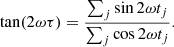
The periodogram can also be used to identify periodicities within our full-polarization light curves, through statistical analysis of the periodogram distribution evaluated at the set of frequencies {ωn = 2πn/Δt, n = 1, 2, …, N/2}, where N is the number of data points in the time series, and Δt is the time length of the light curve, as proposed in Scargle (1982).
The estimation of the PSD and the search for periodicities in radio astronomical light curves present challenges, as these datasets are often characterized by non-uniform sampling. Additionally, identifying and assessing the reliability of a periodicity in a light curve is more difficult in the presence of red-noise signals, which are common in many astronomical sources. Unfortunately, these challenges render the estimates of the PSD slopes, obtained after applying the periodogram to our signals, unreliable. This unreliability is evidenced by the inconsistency with the PSD slopes estimated using the SF, as presented in Table G.1. No periodicities were identified in the periodogram distributions of any of our light curves.
PSD slope estimates of the 2018 ALMA light curves, using the Lomb-Scargle periodogram PLS(ω) and the SF.
G.1. The high-pass filter periodogram
To reduce the sampling-induced noise that negatively impacts PSD estimates in the classic periodogram formulation, we employed the recently proposed HPF periodogram (see Albentosa-Ruiz & Marchili (2024)). This novel periodogram implementation applies a frequency-dependent HPF to the signal, suppressing the variability components of frequencies lower than a given frequency, ω, in the time domain using a data de-trending algorithm before calculating the periodogram value at that frequency.6
The PSD estimates obtained from the HPF periodogram are presented in Table 1 of the main text, for comparison with the SF results. With this new periodogram implementation, we observe a significant improvement in the results, which are now more consistent with the PSD values obtained from the SF analysis. However, due to the higher noise levels in the total intensity light curves on April 21 and especially April 25, retrieving accurate PSD values remains challenging. This is reflected in the high uncertainty of the estimates and the greater discrepancy with the SF results. Notably, we now observe more stable PSD values across the entire campaign for both total and polarized intensity, compared to the SF estimates, as illustrated in Fig. 11.
Appendix H: Polarization properties and accretion rate of Sgr A*
The RM and m′ observables provide insight into the structure of the Faraday depth across the source (e.g., Sokoloff et al. 1998). In Table H.1, we present the polarized observables averaged for each day. For the total flux density, polarized intensity, EVPA and Stokes V, we report the daily averages for one spectral window (spw) from each ALMA sideband: B1 and B4. Additionally, we provide the average spectral index, RM, and depolarization values, derived from the full-Stokes light curves.
Averaged polarization properties and their measured dispersion across the duration (μ ± σ) of the ALMA 2018 Sgr A* light curves.
Following the methodology described in Goddi et al. (2021), we estimated that the EVPA values are accompanied by an uncertainty of ±0.2–0.3 degrees. This level of uncertainty, smaller than the EVPA rotation introduced by the measured RM values across the ALMA frequency coverage (see Fig. 4 and Table H.1), ensures the robustness of the reported RM evolution curves, as the estimated RM values are not dominated by measurement noise. Figure H.1 illustrates the frequency dependence of the EVPA following a λ2 law, validating the reliability of the derived RM evolution curves.
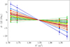 |
Fig. H.1. Sample of Sgr A* EVPA measurements across the four ALMA spectral bands (B1–B4) from the four observing days of the 2018 EHT campaign. The EVPA values for each time sample have been mean-subtracted to emphasize the relative variation across frequency. The dashed lines represent the best-fit linear models of the form ϕ(λ) = ϕ0 − RM(λ2 − λ02), used to estimate the RM evolution curves. |
The RM values inferred in this study introduce an EVPA rotation of approximately 0.5 to 1 degree within each 2 GHz spectral window, and between 5 to 10 degrees across the full ALMA frequency coverage. This rotation can be visualized from the average EVPA in SPWs B1 and B4 (shown in Table H.1). A large EVPA rotation within the observing frequency bandwidth could decrease the measured fractional polarization, resulting in a bandwidth depolarization. Since the EVPA values of Sgr A* do not exhibit such large rotations, we would expect lower depolarization values. However, the RM can arise from three distinct regions, each with a different spatial scale and, as a result, potentially different variability:
-
internal, hot and turbulent plasma from which synchrotron emission originates. Since Faraday rotation decreases significantly as particles become more energetic (Quataert & Gruzinov 2000), this contribution to the RM is sometimes neglected. However, Wielgus et al. (2024) argued that the internal component may be very important in the context of Sgr A*,
-
thermal plasma in the vicinity of the black hole, surrounding the emission region, which has a greater impact on the RM and contributes to short-term variability. This region would also introduce stronger depolarization effects,
-
colder plasma in the most extended and external regions to the black hole, whose effect on RM manifests as long-term variability.
Additionally, Goddi et al. (2021) suggests that, beyond bandwidth depolarization caused by strong magnetic fields, which would manifest as a high RM, three other mechanisms may contribute to the depolarization observed in Fig. 4: Faraday depolarization, beam depolarization, and thermal non-synchrotron emission. The low EVPA rotation due to Faraday rotation observed for Sgr A* suggests that bandwidth depolarization in Sgr A* is likely minimal, and that the observed depolarization may instead arise from these alternative mechanisms.
Analyzing both the rotation measure (RM) and depolarization offers valuable insight into the plasma structure in the immediate vicinity of the black hole. As shown in Fig. 3, both quantities exhibit significant variability, further underscored by the large dispersion relative to their daily averages reported in Table H.1. Properly characterizing the plasma properties, however, requires modeling that can disentangle the contributions of Faraday rotation from those of depolarization. While a detailed investigation of the underlying depolarization mechanisms is beyond the scope of this paper, we do explore the RM and depolarization light curves (see Fig. 4) using the time-series analysis techniques introduced in this work. The lack of significant correlation between the RM and depolarization curves, as indicated by the correlation function analysis, suggests that bandwidth depolarization is unlikely to be the dominant mechanism.
An analysis of variability timescales using the SF reveals distinct timescales in the April 22 light curves. The RM exhibits a characteristic timescale of 32 ± 4 minutes, with a corresponding power spectral density (PSD) slope of −2.26 ± 0.016. This rapid RM variability is consistent with the behavior reported for 2017 data in Wielgus et al. (2024), and supports the interpretation that Faraday rotation originates from an internal screen co-spatial with the compact synchrotron-emitting region near Sgr A*. In contrast, the depolarization light curve displays two prominent timescales: a short one at 15 ± 2 minutes (PSD slope −2.338 ± 0.013), and a longer one at 1.16 ± 0.11 hours (PSD slope −2.485 ± 0.018). This dual-timescale behavior closely resembles that seen in the SF of the Stokes I light curve (see middle panel of Fig. F.1). If bandwidth depolarization were the dominant mechanism, one would expect the depolarization and RM timescales to closely match. The presence of two distinct timescales for depolarization instead suggests that additional or alternative mechanisms may be contributing.
Additionally, we estimated the mass accretion rate Ṁ of Sgr A* (in units of M⊙ yr−1) using our RM measurements and the expression provided in Marrone et al. (2006):
![Mathematical equation: $$ \begin{aligned} \dot{M} =&2.2\cdot 10^{-9} \left[1-\left(\frac{r_\mathrm{out} }{r_\mathrm{in} }\right)^{-(3\beta -1)/2} \right]^{-2/3} \\&\times \left(\frac{M_{BH}}{6.6\cdot 10^9M_\odot } \right)^{4/3} \left(\frac{2}{3\beta -1} \right)^{-2/3} r_\mathrm{in} ^{7/6} RM^{2/3}, \end{aligned} $$](/articles/aa/full_html/2026/04/aa56759-25/aa56759-25-eq34.gif)
where β is a parameter that depends on the accretion flow model, ranging between 1/2 and 3/2; rin and rout represent the inner and outer edges of the Faraday screen (in units of Schwarzschild radius, rs); MBH is the mass of Sgr A*, expressed in M⊙; and RM is given in units of rad⋅m−2. We adopted rin = 3 rs, following the estimated angular size of the emission region reported in Event Horizon Telescope Collaboration (2022a). For simplicity, we took rout → ∞, as its exact value is poorly constrained and has negligible impact on the accretion rate estimate under these assumptions. To derive an upper limit on Ṁ, we use the average RM values measured across the four observing days, ranging from −3 × 10⁵ to −5 × 10⁵ rad⋅m−2 (see Table H.1), and assume β = 3/2. This yields an accretion rate of Ṁ ≈ (2.6–3.9) × 10−9 M⊙ yr−1, which is consistent with expectations from magnetically arrested disk (MAD) models for Sgr A* (e.g., Event Horizon Telescope Collaboration 2022c). The evolution of Ṁ estimated from the RM values at different integration times is shown in Fig. H.2.
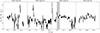 |
Fig. H.2. Sgr A* accretion rate evolution through the ALMA 2018 observations, estimated from the RM light curve presented in Fig. 4, using the accretion flow model presented in Marrone et al. (2006). The gray-shaded band on April 24 marks the time range of the Chandra X-ray flare. |
A more comprehensive analysis, including comparisons with theoretical models and more sophisticated treatments of the Faraday screen geometry, is required to further constrain the plasma conditions around Sgr A* and to better understand the structure of the Faraday-active region near the Galactic Center black hole.
Appendix I: Full polarization 2017 ALMA light curves
The Sgr A* 2017 light curves from the ALMA observations conducted on April 6, 7, and 11 as part of the 2017 EHT campaign, originally published in Wielgus et al. (2022a,b, 2024), were also reprocessed following the updated intra-field calibration presented in Sect. 2.2. We retrieved the full-polarization Sgr A* light curves, for comparison with the 2018 light curves. Figure I.1 shows the complete ALMA light curves of the total flux, polarized intensity, the EVPA, and Stokes V. A summary of the main characteristics of these light curves is given in Table I.1. The presented results demonstrate a high degree of consistency with the original intra-field reduction A1, described in Wielgus et al. (2022a), although the flux density is higher, as a result of an updated QA2 with different calibrators. The modulation indices indicate similar variability, further supported by the PSD estimates and the timescales derived from the SF and periodogram analyses (see Fig. 11).
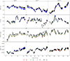 |
Fig. I.1. Sgr A* ALMA light curves of Stokes I, the polarized intensity, the EVPA, and Stokes V (from top to bottom) for the four spectral bands, for all three days (from left to right, 2017 April 6, 7, and 11). Stokes V light curves are tentative, as the detected levels fall below ALMA’s guaranteed CP accuracy. |
ALMA 2017 Sgr A* light curves, in total flux, polarized intensity, and Stokes V.
All Tables
Results from the time-series analysis of the ALMA Sgr A* light curves in total flux density and polarized intensity.
ALMA Sgr A* light curves, in total flux density, polarized intensity, and Stokes V, presented in this paper.
PSD slope estimates of the 2018 ALMA light curves, using the Lomb-Scargle periodogram PLS(ω) and the SF.
Averaged polarization properties and their measured dispersion across the duration (μ ± σ) of the ALMA 2018 Sgr A* light curves.
ALMA 2017 Sgr A* light curves, in total flux, polarized intensity, and Stokes V.
All Figures
|
Fig. 1. Stokes I CLEAN image of Sgr A* and the minispiral from visibilities at 213.1 GHz, produced after the QA2 calibration for April 21. |
| In the text | |
|
Fig. 2. April 22 total flux density of Sgr A* and the minispiral at 213.1 GHz, before (red and blue crosses) and after (purple and black dots) correcting for variability transfer. The flux density uncertainty, estimated from the covariance matrix, is approximately 0.1% and is therefore not visible. |
| In the text | |
|
Fig. 3. Sgr A* ALMA light curves of Stokes I, the polarized intensity, the EVPA, and Stokes V (from top to bottom) for the four spectral bands, for all four days (from left to right, April 21, 22, 24, and 25). Stokes V light curves are tentative, as the detected levels fall below ALMA’s guaranteed CP accuracy. The gray-shaded band on April 24 marks the time range of the Chandra X-ray flare. |
| In the text | |
|
Fig. 4. Sgr A* ALMA light curves of the fractional polarization for the four spectral bands, the depolarization measure, the rotation measure, and the spectral index (from top to bottom) for all four days (from left to right, April 21, 22, 24, and 25). The gray-shaded band on April 24 marks the time range of the Chandra X-ray flare. |
| In the text | |
|
Fig. 5. Historical 230 GHz amplitude measurements of Sgr A* from 2005 to 2019 in Table 4 of Wielgus et al. (2022a) and average flux density and standard deviation from Table E.1. The 2017 and 2018 EHT observing campaigns are marked by black vertical lines. Standard deviations for both the 2017 and 2018 EHT observations are plotted, but are too small to be visible. |
| In the text | |
|
Fig. 6. Modulation index measured across various observations as a function of observational duration. Each data point from the 2018 ALMA dataset at B3 (227 GHz) is represented by hexagons, while other data points, as well as the fitted damped random walk (DRW) curve with shaded confidence intervals are derived from Wielgus et al. (2022a). |
| In the text | |
|
Fig. 7. Modulation indices σ/μ of the Stokes I (top) and polarized intensity (bottom) ALMA light curves, for the 2017 and 2018 observations at B1 (black dots) and B4 (blue diamonds), obtained from our analysis. |
| In the text | |
|
Fig. 8. LNDCF between SPWs B1–B2 (black dots), B1–B4 (red squares), and B3–B4 (blue diamonds), for total flux density (left) and polarized intensity (right), for April 24. |
| In the text | |
|
Fig. 9. LNDCF between ALMA SPWs B1-B4 for all four days, showing total flux density (left) and polarized intensity (right). The dotted lines indicate the delays between SPWs B1–B4 retrieved from the LNDCF. |
| In the text | |
|
Fig. 10. SF plots of the Sgr A* 213.1 GHz light curves for total intensity (left) and polarized intensity (right), for April 21, 22, 24 and 25, and all combined (black dots, blue squares, red diamonds, magenta triangles, and cyan crosses, respectively). |
| In the text | |
|
Fig. 11. PSD slope index (top) and timescales (bottom) estimated from the SF of the total intensity (left) and polarized intensity (right) 2017 and 2018 light curves, for the spectral bands B1 (blue dots) and B4 (orange squares). A second characteristic PSD and timescale, derived from the Stokes I SF, are marked with a cross (x). PSD values are computed from the SF slope as αPSD = −(1 + αSF) (blue dots and orange squares for the spectral bands B1 and B4, respectively), and from the HPF periodogram (red triangles and green diamonds for the spectral bands B1 and B4, respectively; see Appendix G). |
| In the text | |
|
Fig. 12. Sgr A* ALMA polarimetric loops observed in April 2018, for the spectral band B4, for all four days. The colors of the data points represent the time evolution of the Q − U behavior. |
| In the text | |
|
Fig. 13. Chandra counts (top) and Sgr A* total intensity ALMA light curves (bottom) for the flares observed in 2017 and 2018 during the EHT campaigns. The gray-shaded band marks the time range of the high-energy flare, with indicated maximum. |
| In the text | |
|
Fig. 14. Distribution of M3 in ALMA observations taken during the 2017 and 2018 EHT campaigns, compared to the distributions from different GRMHD models. The top panel shows the comparison with the EHT library of GRMHD models, while the bottom panel shows the comparison with the 1T and 2T GRMHD models from Salas et al. (2025). The dark red part of the observational histogram represents the 2017 ALMA data from Wielgus et al. (2022a), and the light red part corresponds to the 2018 results introduced in this paper. |
| In the text | |
|
Fig. A.1. Bandpass of Sgr A* for the April 22 observations indicating the channels impacted by absorption at B3. The bandpass remains virtually unchanged across all days. |
| In the text | |
|
Fig. B.1. Reconstructed visibility-amplitude light curves for the EHT targets obtained with ALMA during the 2018 EHT VLBI campaign: 3C 279 (red circles), M87 (blue triangles), NRAO 530 (green diamonds), and QSO B1921-293 (black squares). |
| In the text | |
|
Fig. C.1. Snapshot of the calibrated data for Sgr A* at 7:23 UTC on April 25 from the SEFD-based data reduction. The colored circles represent the combined visibilities of the minispiral and Sgr A*. The solid colored lines are the mean flux density in each spectral window. The gray-shaded area represents the range of visibilities we consider for the minispiral (0-50 m). The red-shaded area represents the flagging cutoff for the extended structure used by SMA (0-30 kλ). |
| In the text | |
|
Fig. D.1. Sgr A* light curves for ALMA and SMA at all four available bands. |
| In the text | |
|
Fig. F.1. Sample of SF fitted to retrieve the slope (blue line, with an area corresponding to the 3σ level), the plateau level (orange line) and the timescales (red point, marking the intersection of the slope and the plateau). Left: SF of the April 21 Stokes I denoised light curve. Right: SF of the April 22 Stokes I light curve; we note two distinct slopes, fitted independently (the second slope corresponds to the green line). |
| In the text | |
|
Fig. H.1. Sample of Sgr A* EVPA measurements across the four ALMA spectral bands (B1–B4) from the four observing days of the 2018 EHT campaign. The EVPA values for each time sample have been mean-subtracted to emphasize the relative variation across frequency. The dashed lines represent the best-fit linear models of the form ϕ(λ) = ϕ0 − RM(λ2 − λ02), used to estimate the RM evolution curves. |
| In the text | |
|
Fig. H.2. Sgr A* accretion rate evolution through the ALMA 2018 observations, estimated from the RM light curve presented in Fig. 4, using the accretion flow model presented in Marrone et al. (2006). The gray-shaded band on April 24 marks the time range of the Chandra X-ray flare. |
| In the text | |
|
Fig. I.1. Sgr A* ALMA light curves of Stokes I, the polarized intensity, the EVPA, and Stokes V (from top to bottom) for the four spectral bands, for all three days (from left to right, 2017 April 6, 7, and 11). Stokes V light curves are tentative, as the detected levels fall below ALMA’s guaranteed CP accuracy. |
| In the text | |
Current usage metrics show cumulative count of Article Views (full-text article views including HTML views, PDF and ePub downloads, according to the available data) and Abstracts Views on Vision4Press platform.
Data correspond to usage on the plateform after 2015. The current usage metrics is available 48-96 hours after online publication and is updated daily on week days.
Initial download of the metrics may take a while.