| Issue |
A&A
Volume 708, April 2026
|
|
|---|---|---|
| Article Number | A210 | |
| Number of page(s) | 17 | |
| Section | Cosmology (including clusters of galaxies) | |
| DOI | https://doi.org/10.1051/0004-6361/202558719 | |
| Published online | 09 April 2026 | |
The imprints of massive neutrinos on the three-point correlation function of large-scale structures
1
Dipartimento di Fisica e Astronomia “Augusto Righi”, Università di Bologna, Via Piero Gobetti 93/2, I-40129 Bologna, Italy
2
INAF–Osservatorio di Astrofisica e Scienza dello Spazio di Bologna, Via Piero Gobetti 93/3, I-40129 Bologna, Italy
3
INAF-Osservatorio Astronomico di Brera, Via Brera 28, I-20122 Milano, Italy
4
INFN-Sezione di Genova, Via Dodecaneso 33, I-16146 Genova, Italy
5
Dipartimento di Fisica, Università di Genova, Via Dodecaneso 33, I-16146 Genova, Italy
★ Corresponding author: This email address is being protected from spambots. You need JavaScript enabled to view it.
Received:
22
December
2025
Accepted:
25
February
2026
Abstract
Aims. Free-streaming of cosmic neutrinos affects the distribution and growth of cosmic structures on small scales. This enables the sum of neutrino masses Mν to be constrained from clustering studies. We investigate the possibility of disentangling massive neutrino cosmologies with the three-point correlation function (3PCF) for the first time.
Methods. We measured the isotropic connected 3PCF ζ and the reduced 3PCF Q of halo catalogs from the QUIJOTE suite of N-body simulations, considering Mν = 0.0, 0.1, 0.2, and 0.4 eV in different redshift bins. We developed a framework to quantify the detectability of massive neutrinos for different triangle configurations and shapes, and applied it to a case compatible with a stage-IV spectroscopic survey. We also compared our results with the analysis of simulations without neutrinos, but with different σ8 values, to test whether the 3PCF can break the well-known degeneracy between the two parameters.
Results. We found that as a result of free-streaming, the strongest signal is found for quasi-isosceles and squeezed triangles; this signal increases for decreasing redshifts. Among these configurations, elongated triangles, tracing the filamentary structure of the cosmic web, are the most affected by massive neutrinos, with a 3PCF signal increasing with Mν. A complementary source of signal comes from right-angled triangles in Q. Importantly, we found that the signatures of a σ8 variation appear to be significantly different on elongated triangles in ζ and right-angled triangles in Q, suggesting that the 3PCF can be used to effectively break the Mν − σ8 degeneracy. These results open the possibility to use the 3PCF as a powerful complementary tool for constraining neutrino masses in current and future spectroscopic surveys such as DESI, Euclid, 4MOST, and the Nancy Grace Roman Space Telescope.
Key words: astroparticle physics / neutrinos / cosmology: theory / dark matter / large-scale structure of Universe
© The Authors 2026
 Open Access article, published by EDP Sciences, under the terms of the Creative Commons Attribution License (https://creativecommons.org/licenses/by/4.0), which permits unrestricted use, distribution, and reproduction in any medium, provided the original work is properly cited.
This article is published in open access under the Subscribe to Open model. This email address is being protected from spambots. You need JavaScript enabled to view it. to support open access publication.
1. Introduction
Neutrinos have nonzero mass, as first confirmed by the detection of their flavor oscillations (Fukuda et al. 1998), providing clear evidence for physics beyond the standard model, where neutrinos are typically assumed to be massless. This has important implications for cosmology.
According to the Big Bang paradigm, a thermal neutrino relic component, known as cosmic neutrino background, should exist, contributing to the total radiation energy density at early times, when still relativistic, and to the total matter density after the nonrelativistic transition (Lesgourgues & Pastor 2006, for a comprehensive review). Since gravity is sensitive to the sum of neutrino masses Mν ≡ ∑imi, cosmology is complementary to oscillation experiments, which instead measure the splitting of neutrino masses squared Δmi2 in determining the neutrino absolute mass scale, still one of the open problems of particle physics (see Navas et al. 2024, for a comprehensive review). Furthermore, reaching an accurate description of the imprint left by neutrinos on cosmological observables is essential to avoid systematics in the determination of cosmological parameters in current and upcoming spectroscopic surveys, such as the European Space Agency Euclid mission (Euclid Collaboration: Mellier et al. 2025), the Dark Energy Spectroscopic Instrument (DESI; DESI Collaboration 2016), the 4-metre Multi-Object Spectroscopic Telescope (4MOST; de Jong et al. 2019), and the Nancy Grace Roman Space Telescope (Dore et al. 2019).
Due to their low masses, cosmic neutrinos have high thermal velocities even in the nonrelativistic regime; this has a significant effect on structure formation. Perturbations of the massive neutrino density field are indeed washed out on scales smaller than their free-streaming scale λfs (Bond et al. 1980; Lesgourgues & Pastor 2006), which is proportional to the average distance traveled by neutrinos during one Hubble time due to their thermal velocity. For a neutrino species of mass mi, λfs evolves with redshift z according to the relation (Lesgourgues et al. 2013)
 (1)
(1)
where H(z) is the Hubble parameter at redshift z, and H0 is its present-day value. On scales much larger than λfs, neutrinos behave like cold dark matter (CDM).
Since perturbations of the cosmological fluid are the seeds for present-day observable structures, galaxy clustering represents an ideal probe for investigating the imprint of massive neutrinos on structure formation. In this framework, galaxies and the halos in which they reside are treated as tracers of the underlying matter field; the relation between their spatial distribution and the dark matter perturbations is known as the bias relation (Kaiser 1984; Bardeen et al. 1986; Desjacques et al. 2018). The evolution of perturbations and the bias relation were treated perturbatively by introducing linear and nonlinear terms in the dark matter perturbations (Bernardeau et al. 2002, for a comprehensive review), with the latter becoming increasingly relevant on small scales. Moreover, anisotropic effects relative to the line of sight (LOS), both linear and nonlinear, are introduced in the galaxy distribution by the peculiar velocities of galaxies, a phenomenon known as redshift-space distortions (RSDs; Kaiser 1987; Hamilton 1992; Fisher 1995; Scoccimarro et al. 1999; Scoccimarro 2004; Taruya et al. 2010).
The statistical properties of the large-scale galaxy distribution are extracted by measuring the N-point statistics of the density field, starting with two-point statistics, specifically, the two-point correlation function (2PCF) in configuration space and its Fourier transform, the power spectrum, in Fourier space. These statistics quantify the excess or deficit in the probability of finding pairs of galaxies with respect to a random distribution as a function of the distance between the two objects of the pair.
The effect of massive neutrinos on two-point statistics has been extensively studied in configuration and Fourier space. Neutrinos are found to suppress the total matter and CDM power spectra below the free-streaming scale (Hu et al. 1998; Brandbyge et al. 2010; Viel et al. 2010; Castorina et al. 2015; Villaescusa-Navarro et al. 2018), to affect RSDs by inducing a scale dependence in the linear growth rate f and by modifying the root mean square of galaxy peculiar velocities (Marulli et al. 2011; Verdiani et al. 2025), and to induce a scale-dependent bias even at large scales (Villaescusa-Navarro et al. 2014; Castorina et al. 2014). From N-body simulations, Castorina et al. (2014) and Verdiani et al. (2025) proved, respectively, that the linear bias depends solely on the variance of the CDM density field (the so-called universality in the CDM component), and RSDs in the linear regime are better described by assuming that the halo velocity field is unbiased with respect to the CDM velocity field alone. The imprints of massive neutrinos were also studied by cross-correlating cosmic voids and cosmic microwave background (CMB) lensing (Vielzeuf et al. 2023). In addition to small scales, the effect of neutrinos has also been investigated at the scales of baryon acoustic oscillations (BAO; Peloso et al. 2015; Parimbelli et al. 2021), recently focusing on systematics that may arise in neglecting neutrino masses in BAO reconstruction techniques (Nadal-Matosas et al. 2025).
Cosmological analyses routinely use two-point statistics to constrain the sum of neutrino masses, often in combination with CMB data to break parameter degeneracies (e.g., Sánchez et al. 2014, 2017; Grieb et al. 2017; Ivanov et al. 2020; Semenaite et al. 2023; Moretti et al. 2023). The recent analyses from DESI (Adame et al. 2025; Abdul Karim et al. 2025; Elbers et al. 2025), combined with CMB data, yielded very stringent 95% confidence level upper limits of Mν ≲ 0.07 eV while constraining Mν ≲ 0.4 eV from two-point statistics alone.
However, two-point statistics provide a complete statistical description of the galaxy field only under the assumption of a perfectly Gaussian distribution (Bernardeau et al. 2002). To quantify the non-Gaussian properties of the large-scale structure, higher-order statistics, such as the three-point correlation function (3PCF; Peebles 1980; Fry & Gaztanaga 1993; Frieman & Gaztanaga 1994; Jing et al. 1995; Jing & Börner 2004) and its Fourier-space counterpart, the bispectrum (Fry 1984; Scoccimarro et al. 1999; Sefusatti et al. 2006), are needed. Many sources of non-Gaussianity indeed act on the galaxy distribution, originating from nonlinearities involving the growth of perturbations (Fry 1984), RSDs (Hivon et al. 1995; Scoccimarro et al. 1999), and galaxy bias (Fry & Gaztanaga 1993; Fry 1994; Frieman & Gaztanaga 1994), and potentially from several inflationary scenarios (Verde et al. 2000; Celoria & Matarrese 2018; Meerburg et al. 2019). In particular, nonlinear effects, with their associated non-Gaussianity, are dominant on small scales. Since these scales are those on which neutrinos leave most of their characteristic signatures, statistics that quantify non-Gaussianity (i.e., higher-order ones) can be used to extract additional information with respect to lower-order ones.
Furthermore, two-point statistics are affected by degeneracies between parameters, in particular, by a strong degeneracy between Mν and the cosmological parameter σ8 (e.g., Viel et al. 2010; Villaescusa-Navarro et al. 2018), the latter defined as the present-day standard deviation of the linear matter density field on a conventional scale of 8 h−1 Mpc. This degeneracy limits the possibility of obtaining precise constraints on Mν from two-point statistics alone and requires exploring also higher-order statistics.
The first measurement of a bispectrum from N-body simulations including massive neutrinos was published in Ruggeri et al. (2018), quantifying the neutrino-induced suppression on the bispectrum and proving universality in the CDM component also beyond linear bias. The study of the halo and galaxy bispectrum from mock catalogs up to small scales proved its power in breaking degeneracies (including the Mν − σ8 degeneracy) and tightening cosmological parameter constraints compared to the power spectrum alone (Hahn et al. 2020; Hahn & Villaescusa-Navarro 2021; Kamalinejad & Slepian 2025, 2026).
Early studies of 3PCF only focused on specific configurations (Gaztañaga et al. 2005; McBride et al. 2011; Marín et al. 2013; Moresco et al. 2014) or on the detection of acoustic features (Gaztañaga et al. 2009; de Carvalho et al. 2020; Moresco et al. 2021), due to the high computational cost required by measures that rely on direct triplet counts. The introduction of an estimator based on spherical harmonic decomposition (SHD; Slepian & Eisenstein 2015a, 2018) has significantly reduced the computational cost, enabling more systematic analyses (Slepian et al. 2017a,b, 2018). Another computational bottleneck concerns the modeling of the 3PCF, which is obtained by Fourier-transforming bispectrum models. While some perturbative approaches exploit one-dimensional fast Fourier transforms (FFT) at leading order (Slepian & Eisenstein 2017; Sugiyama et al. 2021), more general methods require two-dimensional FFT (Fang et al. 2020) to perform the inversion (Umeh 2021; Guidi et al. 2023; Pugno et al. 2025; Farina et al. 2026). The computational times of these approaches for sampling the parameter space properly are prohibitively long. This issue, however, can be overcome by developing emulators (Euclid Collaboration: Guidi et al. 2026).
In this evolving context, a systematic study of the effects of massive neutrinos on the 3PCF is still lacking. In addition to complementing bispectrum analyses, bridging this gap is crucial because configuration-space statistics are less sensitive to possible systematics arising from survey geometry, which instead introduce additional mode coupling in Fourier space that is far more challenging to account for in the modeling and estimators (Philcox 2021; Pardede et al. 2022).
We focus on the measurements of the halo 3PCF obtained from a large number of mock catalogs from N-body simulations that include a massive neutrino component. This represents the first measurement of 3PCF in simulations implementing massive-neutrino cosmologies. In particular, we search for and quantify the signatures imprinted by massive neutrinos on the 3PCF, and we identify the structures that maximize the detectability of a potential neutrino signal by taking advantage of the power of the 3PCF to infer clustering as a function of the triangle scale and shapes. Moreover, we exploit this capability to disentangle the effect of massive neutrinos from variations in σ8.
This paper is organized as follows. In Sect. 2 we provide an overview of the methods and data employed in this analysis, defining the adopted statistics (2.1) and describing the set of simulations used (2.3), the estimators considered (2.2), the dataset produced from the measurements together with the estimation of covariance (2.4), and the framework developed for the neutrino detectability analysis (2.5). In Sect. 3 we present our results, focusing on the triangle scale (3.1 and 3.2) and shape (3.3) dependence of the signal from massive neutrinos, and the possibility of breaking the Mν − σ8 degeneracy with the 3PCF (3.4). Finally, in Sect. 4 we draw our conclusions.
2. Methods and data
2.1. Clustering statistics
The probability dP of finding a triplet of objects inside the comoving volumes dV1, dV2, and dV3, separated by the comoving distances s12, s13, and s23, can be written as
![Mathematical equation: $$ \begin{aligned} \begin{aligned} {\mathrm{d} } P = \bar{n}^3 \, [ 1 + \xi (s_{12}) + \xi (s_{13}) + \xi (s_{23}) + \zeta (&s_{12}, s_{13}, s_{23})] \\&{\mathrm{d} } V_1{\mathrm{d} } V_2{\mathrm{d} } V_3\; , \end{aligned} \end{aligned} $$](/articles/aa/full_html/2026/04/aa58719-25/aa58719-25-eq2.gif) (2)
(2)
where  is the average number density of objects, and ξ and ζ, are the 2PCF and connected 3PCF, respectively (Peebles 1980). Unlike the 2PCF, which only encodes scale information (being exclusively dependent on the separation between pairs of objects), the 3PCF is the lowest-order clustering statistics able to also provide information about the shape of structures (since size and shape both characterize triangles).
In redshift space, ξ and ζ also depend on the orientation between a given pair or triplet, respectively, and the LOS unit vector  due to the action of RSDs, which break the assumption of isotropy by introducing the privileged direction defined by
  . This splits clustering statistics into an isotropic component, defined by averaging them in redshift space over all the possible LOS directions, which solely depends on pair/triplet separations, and an anisotropic component that retains the specific directional dependence. We only focus on the isotropic component of the statistics we considered here and aim to extend it with anisotropic information in a future work.
We complemented the information provided by the isotropic 3PCF by also considering the reduced 3PCF Q (Groth & Peebles 1977), defined as
 (3)
(3)
where ξ0 denotes the monopole of the 2PCF (i.e., the isotropic component of the 2PCF). The reduced 3PCF provides a natural combination of ζ and ξ; since it can be demonstrated that in hierarchical scenarios, ζ ∝ ξ2 to a good approximation (Peebles & Groth 1975), this quantity is on the order of unity on all scales by definition, and it is explicitly independent of σ8 by construction (see Eq. 6 in Moresco et al. 2021).
2.2. Estimators
We estimated the 2PCF with the natural estimator (Peebles 1973)
 (4)
(4)
where μ is the cosine of the angle between the pair and the LOS direction, and DD and RR are the pair counts in the data and in a random distribution of unclustered objects with the same geometry as the data catalog, respectively. In our case, that is, a simulation box with periodic boundary conditions (as detailed in Sect. 2.3), this estimator is equivalent to the usual Landy-Szalay estimator (Landy & Szalay 1993). Moreover, periodicity allowed us to compute the RR term analytically. We then obtained the 2PCF monopole by numerically averaging  over μ.
We estimated the isotropic connected 3PCF with the SHD estimator introduced in Slepian & Eisenstein (2015a), which has the advantage of scaling with the number of objects N as 𝒪(N2), rather than 𝒪(N3), as in the case of previous estimators relying on direct triplet counts. This approach is based on parameterizing a given triangle of sides s12, s13, and s23 with two of its sides, for example, s12 and s13, and the angle θ between them. The third side s23 is then reobtained as a function of s12, s13, and θ. This parameterization allowed us to expand the dependence of the isotropic 3PCF ζ(s12, s13, θ) on θ into Legendre polynomials (Szapudi 2004), with coefficients given by the corresponding Legendre multipoles ζℓ(s12, s13) (see Eq. 11 in Euclid Collaboration: Guidi et al. 2026). Therefore, the full estimator  for the connected 3PCF can be written as a function of an estimator
  for the isotropic Legendre multipoles as
 (5)
(5)
where ℓmax is the highest-order multipole included in the expansion. The isotropic multipoles are estimated as
 (6)
(6)
where DDDℓ, DDRℓ, DRRℓ, and RRRℓ are the multipoles of the Legendre expansion of the data-data-data, data-data-random, data-random-random, and random-random-random triplet counts, respectively. This expression is analogous to the traditional Szapudi & Szalay (1998) direct triplet count estimator, applied to the case of the 3PCF multipoles. The evaluation of the terms in Eq. (6) was detailed in Slepian & Eisenstein (2015a). Again, the periodicity of the simulation box allows for the analytical computation of the monopole of the random counts RRR0.
The efficiency of the SHD estimator is reduced for nearly isosceles triangle configurations (s12 ≃ s13), since a much larger number of multipoles (ℓmax > 30) are needed to properly reconstruct the shape of ζ when θ → 0 (e.g., Veropalumbo et al. 2021). For this reason, we adopted the quantity introduced by Veropalumbo et al. (2022),
 (7)
(7)
which can be used to exclude, by setting η > ηmin, triangles that progressively deviate from the isosceles configuration (see also Guidi et al. 2023; Euclid Collaboration: Guidi et al. 2026; Farina et al. 2026). For our measurements, we used the implementation of the estimators in Eqs. (4) and (5) provided in the publicly available software MeasCorr1 (Farina et al. 2026).
2.3. Simulation dataset
We used the QUIJOTE2 suite of N-body simulations (Villaescusa-Navarro et al. 2020), which provides a large number of realizations to assess the effect on several statistics of variations in the cosmological parameters and to estimate covariance matrices. They were run using the tree particle mesh-smoothed particle hydrodynamics code GADGET-III (Springel et al. 2005). The suite contains massless- and massive-neutrino simulations, whose main properties we describe below.
The fiducial cosmology of the simulations corresponds to a flat ΛCDM Universe with cosmological parameters in agreement with the latest constraints by Planck (Planck Collaboration VI 2020). In particular, it is characterized by the sum of neutrino masses Mν = 0 eV and σ8 = 0.834. Massive-neutrino simulations assume three degenerate neutrino masses and were implemented by using the particle-based method (Brandbyge et al. 2008; Viel et al. 2010), in which neutrinos are described as a collisionless and pressureless fluid discretized into particles. The simulations we considered followed the evolution of 5123 CDM particles plus, if Mν ≠ 0, 5123 neutrino particles, in a periodic cubic box of side length L = 1 h−1 Gpc, and have a softening length of 50 h−1 kpc. The initial conditions (ICs) of the simulations were generated at zi = 127. Displacements and peculiar velocities of particles were computed either with the Zeldovich approximation (ZA; Zel’dovich 1970) or with the second-order Lagrangian perturbation theory (2LPT; Bernardeau et al. 2002) in massive and massless neutrino models, respectively. In addition to peculiar velocities, neutrino particles were assigned thermal velocities randomly drawn from a Fermi-Dirac distribution at zi. Halos were identified by running the friend-of-friends algorithm (Davis et al. 1985) with a linking length parameter b = 0.2 on the CDM particles. Only halos containing at least 20 CDM particles were saved, corresponding to a minimum halo mass Mmin ≈ 1.3 × 10¹³ h−1 M⊙.
We considered massive neutrino simulations that were run for three different values of Mν = 0.1, 0.2, and 0.4 eV (with the remaining cosmological parameters fixed at their fiducial values), labeled Mnu_p, Mnu_pp, and Mnu_ppp respectively (500 realizations per simulation). The z = 0 values of the free-streaming scale in these cosmologies according to Eq. (1) are λfs ∼ 240, 120, and 60 h−1 Mpc for Mν = 0.1, 0.2, and 0.4 eV, respectively (where we assumed mi = Mν/3), with only a ∼10% variation in the redshift range 0 ≤ z ≤ 2 relevant for this work assuming the QUIJOTE cosmology.
To study the degeneracy between Mν and σ8, we complemented this set with massless-neutrino simulations differing from the fiducial cosmology only in the value of σ8, with σ8 = 0.849, and σ8 = 0.819, labeled s8_p and s8_m, respectively (500 realizations per simulation). The control sample of the massive-neutrino and varying-σ8 simulations was made of two sets of 500 realizations each of the fiducial cosmology, run with ZA and 2LPT ICs, and labeled fiducial and fiducial_ZA. We also included 2000 additional realizations of the fiducial cosmology run with 2LPT ICs for the numerical estimation of covariance. For all the realizations, we moved halos to redshift space by computing RSDs along the  axis of the simulations.
2.4. Measurements and covariance
We measured the 2PCF monopole for the halo catalogs of the simulations listed in Sect. 2.3 at z = 0, 1, 2. For these redshifts, the number of halos identified in each realization is ∼4 × 10⁵, 2 × 10⁵, and ∼4.4 × 10⁴. We chose separations ranging from smin = 1 h−1 Mpc to smax = 150 h−1 Mpc and linearly spaced bins of width Δs = 1 h−1 Mpc and Δμ = 0.01. For the connected 3PCF, we included all triangles with side lengths from smin = 2.5 h−1 Mpc to smax = 147.5 h−1 Mpc, considering a bin width Δs = 5 h−1 Mpc, and we estimated the isotropic multipoles ζℓ up to ℓmax = 10, which for the vast majority of triangle configurations represents an optimal balance between computational cost and information content.
For each set of simulations, we averaged the measured multipoles over the different realizations and followed two approaches. In the first approach, which we refer to as the single-scale approach, we fixed two triangle sides s12 and s13 and computed ζ(s12, s13, θ) and Q(s12, s13, θ). We obtained the average  for each set of simulations by substituting the average multipoles in Eq. (5), and we used it together with the average 2PCF monopole in Eq. (3) to obtain the average
  . In the second approach, we computed the average
  and
and  of each simulation set for all the possible side-binned triangles obtained by adopting the ordering s12 ≤ s13 ≤ s23. We refer to this scheme as the all-scales approach.
To evaluate the denominator of Q, we linearly interpolated the average 2PCF monopole at the values of s12, s13, and s23 in Eq. (3) in both approaches. Moreover, since the 2PCF monopole changes sign for s ∼ 120 h−1 Mpc, the denominator of Q can exhibit zero crossings when at least one triangle side is above this scale. However, the separation s at which ξ0 changes sign depends on the realization. We therefore inserted already averaged quantities in Eq. (3) instead of averaging after estimating Q for each realization. As an additional precaution, we restricted the analysis of the reduced 3PCF to configurations for which all sides are smaller than 110 h−1 Mpc, in which case the average monopole of the 2PCF remains positive.
We numerically estimated the covariance matrix of the multipoles of the 2PCF and 3PCF from the 2000 fiducial mocks. The 3PCF multipole covariance depends on two triangle side pairs p = (s12, s13), p′ = (s12′,s13′) and two multipole indexes ℓ, ℓ′, so we denoted it with  . The single-scale and all-scales covariance matrices can then be obtained as
 (8)
(8)
 (9)
(9)
with t = (s12, s13, s23), t′ = (s12′,s13′,s23′). We rescaled all covariances in a volume of 10 h−3 Gpc3, taken as an ideal representative of a redshift bin of a stage-IV survey (Albrecht et al. 2006) at z ∼ 1, such as for the Euclid Wide Survey (Euclid Collaboration: Scaramella et al. 2022). We estimated that even extending it to lower or higher redshifts does not significantly affect our findings. All the measurements of 3PCF obtained for this analysis are available among the data products of the QUIJOTE suite3.
2.5. Detectability metrics
The simplest parameter we defined to quantify the neutrino signal is an error-weighted difference, which we simply refer to as detectability,
 (10)
(10)
where the numerator is the difference between the averages of a given statistics (e.g., the average  or
or  ), estimated in one of the massive-neutrino cosmologies and in the fiducial cosmology from the fiducial_ZA mocks. This parameter provides an estimate of the detectability in a specific configuration identified by the index i, denoting a generic bin in which the difference is evaluated. The error is obtained as
  , where
  is the covariance matrix of f.
We also generalized the element-wise detectability in Eq. (10) by introducing a metric that estimates the detectability over a given range of configurations, accounting for their correlation, defined by the parameter
 (11)
(11)
where i and j run on the angles formed by s12 and s13, and the differences  , with
  or
or  , are defined in the same way as in the numerator of Eq. (10). We defined this parameter
  in analogy with the standard definition of the reduced chi-squared, except that in place of the model, we inserted the estimated fiducial statistic.
This parameter also allowed us to provide a quantitative assessment of the statistical significance of the signal from neutrinos of total mass Mν. In particular, it is possible to compute the p value associated with a given value of  , that is, the tail integral of a chi-squared distribution ℱ(χ2; Nθ) with Nθ degrees of freedom,
 (12)
(12)
and then convert it into an equivalent Gaussian statistical significance Zσ, where Z is implicitly defined as follows (Cowan et al. 2011):
 (13)
(13)
Here, 𝒩 is the standard Gaussian distribution, characterized by zero mean and unitary variance.
To account for the fact that the precision matrix obtained by inverting a numerically estimated covariance matrix is a biased estimator of the parent population precision matrix, we applied the correction factor prescribed by Hartlap et al. (2007). This consists of multiplying each inverse covariance matrix by the factor (Nm − nd − 2)/(Nm − 1), where Nm is the number of mocks used to estimate the covariance, and nd is the dimensionality of the data vector.
As a final note, we emphasize that although the various indicators defined may appear quite different, they are all based on the same underlying principle, quantifying the deviation of a given measurement from the fiducial one, weighted by the associated uncertainty. However, depending on the case, it is useful to use one or the other, as they provide complementary information.
3. Results
We estimated the detectability of massive neutrinos in different configurations. Below, we present our main results, starting with the 3PCF analysis in single-scale configurations and then moving to the all-scales approach.
3.1. Single-scale analysis
We computed the parameter  defined in Eq. (11) for all the values of Mν and redshift. The covariance matrix (Eq. 8) is singular if Nθ > ℓmax + 1. For this reason, we chose to estimate ζ in ten evenly spaced angular bins, with 0 ≤ θ ≤ π. For Q, we excluded the first bin, corresponding to θ = 0. This ensured that the third side s23 was not smaller than the minimum separation at which we measured the 2PCF monopole, required for its interpolation.
We show the results for ζ in Fig. 1 for the illustrative case Mν = 0.4 eV at all redshifts. As a general trend, we find that the detectability of neutrinos increases as the redshift decreases. At a given redshift, it appears mostly concentrated in specific triangle configurations, identified by the brightest colors in the figure. A first set of configurations is defined by the isosceles ones (i.e., the diagonal of the matrix) at small scales, up to s12 = s13 ∼ 30 h−1 Mpc. This is particularly evident considering the results for z = 2. Conversely, the signal drops on larger scales, due to an increase in the variance of the multipoles used to reconstruct the angular dependence of ζ, as detailed in Appendix A. Other configurations that show high values of  are quasi-isosceles (s12 ≈ s13) and squeezed triangles (s13 ≫ s12). These configurations correspond to the two regions close to the diagonal, and to the areas adjacent to the left and lower sides of the figure, respectively, except for the bottom left corner (where s12 and s13 are both small) in the squeezed case.
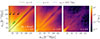 |
Fig. 1. Values of the parameter |

The behavior in the detectability of the neutrino signal in the 3PCF can be explained as a consequence of free-streaming. For a fixed amplitude of the primordial density fluctuations As, high neutrino masses produce lower values of σ8, since the suppression of the matter clustering below λfs is stronger. However, the massive-neutrino simulations of the QUIJOTE suite were created with fixed σ8 = 0.834, hence with a larger As for increasing Mν (in detail, 109As = 2.13, 2.25, 2.40, and 2.74 for Mν = 0.0, 0.1, 0.2, and 0.4 eV, respectively). As a leading effect, the different values of As result in an overall rescaling of all clustering statistics, with scaling factor depending on Mν. This implies that the differences between the 3PCF measured in the massive- and massless-neutrino cases are larger, therefore increasing the detectability, when the 3PCF takes higher values. This occurs on small scales, while on larger scales, where nonlinear effects become negligible, the 3PCF values drop rapidly. This picture is consistent with the overall increase in the  values as z decreases, and with the configurations that maximize it at fixed redshift, since isosceles, quasi-isosceles, and squeezed triangles are precisely those for which at least one of the three sides can probe nonlinear or mildly nonlinear scales. As further confirmation, moving toward the bottom-left corner of the figures, the values of
  increase, reflecting the fact that in this case, all three sides become progressively smaller.
The results obtained for the reduced 3PCF are shown in Fig. B.1. With respect to the connected 3PCF, the neutrino detectability for the reduced 3PCF is lower overall because the errors from the propagation of the uncertainties on ζ and ξ are larger. At all redshifts, the highest values of  are localized in isosceles configurations and increase moving from large to small scales.
In Fig. 1 we identify some sets of configurations from the regions in which the signal is maximized, corresponding to the lines shown in the leftmost panel, with equations η = 0, η = 4, and the vertical line s12 = 10 h−1 Mpc. To visually inspect the effect of neutrinos directly on the 3PCF, we chose some specific configurations, on and off the identified lines, for comparison, corresponding to (s12, s13) = (10, 100),(30, 100),(55, 100), and (30, 50) h−1 Mpc; these are shown in the figure with the numbered markers. For these, we show in Fig. 2 the single-scale connected 3PCF at z = 0 for all the neutrino masses Mν as a function of the third side s23 and their detectabilities. Additionally, we show the measured multipoles ζℓ(s12, s13) from which the functions were estimated. We avoid showing ζ for (s12, s13) with η = 0 because the reconstruction provided by the SHD estimator is, as expected, not accurate. In particular, ζ is characterized by a strong steepening for s23 → 0 (or equivalently, for θ → 0), which cannot be accurately reconstructed by ℓmax = 10 (e.g., see Fig. 2 in Veropalumbo et al. 2021). The three leftmost configurations in Fig. 2 show an optimal reconstruction for ℓmax = 10, since the signal encoded by the highest multipoles is negligible with respect to the lowest ones. For (s12, s13) = (30, 50) h−1 Mpc (rightmost panel), the first ten multipoles still provide a good reconstruction of ζ, although a small amount of residual signal remains confined to ℓ > 10.
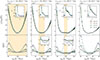 |
Fig. 2. Single-scale connected 3PCF for the triangle configurations selected in Fig. 1 (upper plots of each panel), as indicated in the top label. We show the results at z = 0, with a different color for each neutrino mass, as indicated in the legend. The inset plots in the upper row show the multipoles ζℓ(s12, s13) from which the 3PCF was reconstructed. The lower plots show the corresponding detectabilities as a function of s23 (Eq. 10). The dashed blue line marks the zero detectability level. The orange shaded areas show the region 90 h−1 Mpc ≤ s23 ≤ 110 h−1 Mpc, corresponding to the expected location of the BAO peak. Where the BAO scales do not cover the full s23 range, we include a zoom-in on the detectability in that region to better visualize the effect of neutrinos in those ranges. |
From the detectability plots, it is evident that the signal is captured mainly by configurations that minimize or maximize s23, corresponding to the angles θ = 0 and θ = π. This implies that the signal is mostly driven by elongated triangles, tracing the filamentary structure of the cosmic web. For intermediate values of s23, each mass is either not detectable (as in the case s12 = 10 h−1 Mpc, s13 = 100 h−1 Mpc, where DET ≈ 0 for s23 ≈ 100 h−1 Mpc) or only poorly detectable, with negative detectability values, meaning that ζ(Mν) < ζ(Mν = 0), as in the case of (s12, s13) = (30, 50) h−1 Mpc.
An analogous plot for the single-scale reduced 3PCF is shown in Fig. B.2. Although the neutrino signal is, as previously noted, smaller in amplitude, the behavior of Q as a function of Mν differs substantially from that of ζ. In particular, Q becomes flatter as Mν increases. This produces a different detectability profile as a function of the third side, with negative values for filamentary configurations and positive values for intermediate, more rounded configurations. The same profiles show that the signal is equally driven by filamentary and intermediate configurations, complementary to the behavior obtained with ζ, where the signal is instead largely dominated by the contribution of filamentary structures.
We also inspected the specific contribution of the signal of massive neutrinos at BAO scales. The single-scale 3PCF exhibits a small peak at s23 ∼ 100 h−1 Mpc when, for increasing θ, the two fixed sides s12 and s13 allow the third side s23 to cross the BAO scales (Gaztañaga et al. 2009). This peak has a nontrivial interplay in defining the shape of the 3PCF, possibly canceling out with the 3PCF dip, giving ζ a flat shape for θ ∼ π/2, or resulting in a small peak embedded in the dip, depending on the considered configuration. The behavior is related to the angular spreading of the feature. A smaller angular spreading indeed implies a higher visibility of the peak (Moresco et al. 2021). Equivalently, the visibility of the peak is higher when BAO scales are mapped in a smaller range of s23.
We explicitly chose the configurations (s12, s13) = (10, 100),(30, 100), and (55, 100) h−1 Mpc, so that the BAO feature was progressively concentrated in a smaller s23 range, highlighted in light orange in Fig. 2. For (s12, s13) = (10, 100) h−1 Mpc, the area spans the entire s23 interval, so no distinctive feature is observable. For (s12, s13) = (30, 100) h−1 Mpc, ζ is flatter at the minimum with respect to the previous case, without showing any local maximum, and an extremely shallow peak is visible in the Mν = 0.1 eV detectabilities at ∼100 h−1 Mpc. Finally, for (s12, s13) = (55, 100) h−1 Mpc, a small peak is visible in ζ for all the values of Mν and in the detectabilities of Mν = 0.4 and 0.1 eV. However, we cannot derive any statistically significant effect of the dependence of the amplitude of the BAO feature on Mν because the uncertainties on ζ in the BAO region are too large. We note that even increasing the effective volume to Veff = 500 h−3 Gpc3 does not allow a statistically significant detection at those scales.
In Q, we do not identify any distinctive BAO feature. This is due to the adopted scale cut discussed in Sect. 2.4, which spreads any possible BAO signal over a large portion of the s23 range (as in the case of the leftmost panel in Fig. 2).
3.2. Scale dependence of the neutrino signal
Given the overall decrease in neutrino detectability at smaller scales in Fig. 1, it is relevant to quantify the scales at which the statistical significance of the neutrino signal reaches a given threshold, as a function of neutrino mass, redshift, and configuration set, when moving from the largest scales considered in our analysis to progressively smaller ones. Equations (12) and (13) allow us to convert the  values into the statistical significance of the signal as a function of the triangle sides s12 and s13. We performed this conversion considering the sets of configurations marked with lines in Fig. 1, which we found to encode most of the information content from neutrinos. For this analysis, we identified the characteristic scale scross at which, starting from smax = 147.5 h−1 Mpc and moving toward smaller scales, the statistical significance first reaches 1σ and then 3σ thresholds. We recall that lower p values correspond to higher significances. For a given combination of Mν, redshift, and configurations, the scale scross can therefore be derived as a function of the statistical significance Nσ as
![Mathematical equation: $$ \begin{aligned} s_{\mathrm{cross} }(N\sigma ) \equiv \min \left\{ s \in [s_{\min }, s_{\max }] \, \Big | \, p(s) \ge p(N\sigma ) \right\} \; , \end{aligned} $$](/articles/aa/full_html/2026/04/aa58719-25/aa58719-25-eq42.gif) (14)
(14)
where the scale s can equivalently be considered as either s12 or s13 (since one side is a function of the other side along the specified lines), N = 1 or 3 for 1σ or 3σ significance, respectively, and p(Nσ) is just the p value corresponding to Nσ significance. This value therefore represents an upper limit on the scales that need to be included to obtain a given significant detection of neutrinos: the larger this scale, the easier the neutrino effects are detected; the lower it is, the more scales need to be included for a significant detection.
The results are shown in Fig. 3 for the connected 3PCF in the form of matrices whose elements report the values of scross as a function of Mν and z. For isosceles and quasi-isosceles configurations, we set s = s12, while for configurations with fixed s12 = 10 h−1 Mpc we set s = s13. Overall, a given significance threshold is reached at progressively larger scales for increasing neutrino masses or decreasing redshift, as evident from the increasing values of scross moving from the upper matrix row or the leftmost column (associated with z = 2 and Mν = 0.1 eV, respectively) toward the lower-right matrix element (corresponding to Mν = 0.4 eV and z = 0). We obtained that only the total masses Mν = 0.2 eV and Mν = 0.4 eV are detectable above the 1σ threshold. The mass Mν = 0.2 eV crosses the 1σ significance at all redshifts for configurations with s12 = 10 h−1 Mpc, remaining always below 3σ. The 3σ threshold is reached for isosceles triangles, but only at the smallest scales probed in our analysis, that is, for s12 ∼ 5 h−1 Mpc. For quasi-isosceles triangles with η = 4, this mass has a significance above 1σ for s12 ≲ 40 h−1 Mpc only at z = 0. Our highest mass Mν = 0.4 eV alone is detectable above 3σ at all redshifts for isosceles and squeezed configurations. For these latter, this mass value is already above 1σ on the largest scale probed in our analysis (147.5 h−1 Mpc), unlike for the other masses. For η = 4, the signal crosses 3σ starting from z = 1.
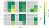 |
Fig. 3. Detectability matrices of massive neutrinos. Each matrix element shows the scale scross (Eq. 14) below which, considering all triangles with a scale larger than scross, we obtained a significant detection of the signal from massive neutrinos in the connected 3PCF. The matrices in the upper and lower rows show the values for a 1σ and 3σ statistical significance (Eq. 13), respectively, computed for a volume of 10 h−3 Gpc3. In each matrix, Mν increases from left to right, and redshifts increase from bottom to top. We show the results for the three configurations corresponding to the lines in Fig. 1, i.e., from left to right: triangles with s12 = 10 h−1 Mpc, isosceles triangles (η = 0), and quasi-isosceles triangles with η = 4. The quantity scross represents one of the two sides, s12 or s13, depending on the configuration: in particular, in Eq. (14) we set s = s13 for triangles with fixed s12, and s = s12 for isosceles and η = 4 triangles. Brighter colors represent better detection levels, i.e., occurring at larger scales. The label ND stands for “not detectable” above the specified significance threshold at any scale. A lower limit is indicated whenever the signal is detectable above a given threshold of statistical significance over the entire range of scales considered in our analysis. |
The analogous results for the reduced 3PCF are shown in Appendix C. The overall behavior is that for a fixed neutrino mass, redshift, and configuration, a given statistical significance threshold is reached at smaller scales with respect to ζ, confirming the lower detectability of Q with respect to ζ.
3.3. Sensitivity of structure shapes to the neutrino signal
We also performed an analysis aimed at quantifying the detectability of massive neutrinos in the 3PCF as a function of triangle shapes. This is particularly relevant because it leverages information on the morphology of cosmic structures that is not accessible at the two-point level.
The single-scale approach, although effective in examining clustering on a given scale for varying triangle configurations, does not allow an efficient isolation of the contribution from triangles of fixed shape. For instance, if s12 and s13 are chosen such that s12 ≪ s13 or s12 ≫ s13, then squeezed triangles are obtained for low and high values of θ. The all-scales approach, by ordering the sides of triangles, such that s12 ≤ s13 ≤ s23 (as detailed in Sect. 2.4), allows for a clear shape classification based on the values assumed by two independent side ratios, as we discuss below.
A useful tool for shape analysis is a particular triangular-shaped plot already adopted in Fourier space (e.g., Takahashi 2014; Desjacques et al. 2018; Hahn et al. 2020; Oddo et al. 2021). In Fig. 4 we derive its configuration-space counterpart for the first time for the connected and reduced 3PCF. We produced this plot for all combinations of neutrino masses and redshift. In the figure, we show the case Mν = 0.4 eV at z = 0, which corresponds to the highest detectability. In this figure, triangle shapes are binned according to the values of the ratios of the smallest and largest side s12/s23 and between the intermediate and largest side s13/s23. The allowed values of s12/s23 and s13/s23 occupy the triangular-shaped region bounded by the vertices (s12/s23, s13/s23) = (0, 1),(1/2, 1/2) and (1, 1). Triangles along the leftmost side of this region have elongated shapes (s23 ≈ s12 + s13), from squeezed (s12 ≪ s13 ≈ s23) in the upper left corner to folded (s12 ≈ s13 ≈ 2 s23) in the bottom corner, while in the top right corner, we find equilateral triangles. We report a visual legend in the upper right panel to facilitate the interpretation of the figure. It is also interesting to focus on right-angled triangles, residing along the dotted line shown in the bottom right panel (the circular arc with equation s232 = s122 + s132). The color of a given shape bin (i.e., a given pixel) represents the absolute value of the detectability of massive neutrinos defined in Eq. (10), averaged over all triangles with that specific shape in a given range of scales. In the various columns, we show the results for three different ranges of s23: the entire range, including all triangles (5 h−1 Mpc ≤ s23 ≤ 145 h−1 Mpc for ζ and 5 h−1 Mpc ≤ s23 ≤ 110 h−1 Mpc for Q), low to intermediate values (5 h−1 Mpc ≤ s23 ≤ 70 h−1 Mpc for ζ and Q), and high values (70 h−1 Mpc ≤ s23 ≤ 145 h−1 Mpc for ζ and 70 h−1 Mpc ≤ s23 ≤ 110 h−1 Mpc for Q).
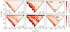 |
Fig. 4. Detectability of the halo connected 3PCF (upper panels) and reduced 3PCF (lower panels) as a function of the triangle shape. The results are reported at z = 0 and for Mν = 0.4 eV. The triangle shapes are determined by the side ratios s12/s23 and s13/s23, with s12 ≤ s13 ≤ s23. In each panel, each pixel represents a given triangle shape, where the color shows the absolute value of the detectability averaged over all the triangles available in the all-scales approach with that shape and different sizes. As shown in the legend in the upper right panel, the bottom center, upper right, and upper left parts of the plot contain folded, equilateral, and squeezed triangles, respectively. The dotted curve in the lower right panel marks the location of right-angled triangles. The white region corresponds to the area in the parameter space where it is not possible to obtain a closed triangle. The various columns differ by the range of s23 considered, specified in the intervals shown in the bottom right corner (in units of h−1 Mpc). Empty bins are colored in gray. |
For ζ, as shown in the upper left plot in the figure, which includes all the triangles considered in our analysis, the most affected regions are those corresponding to the left oblique side of the triangular region, containing elongated triangle shapes transitioning from folded to squeezed. The plots in the middle and right columns show that this feature arises from the combined behavior of triangles belonging to the two s23 ranges. For small to intermediate scales, a comparable contribution to this feature comes from folded and squeezed shapes, also extending to less elongated triangles (i.e., also toward the more central regions of the plot). For larger s23, the detectability pattern on the left oblique side of the plot concentrates on squeezed configurations.
These changes are naturally explained by considering that higher detectability values in ζ identify triangles for which at least one side is small. For triangles with low to intermediate values of s23, this is indeed possible for the squeezed and folded shapes, for instance, for triangles like (s12, s13, s23)∼(5, 5, 10),(10, 10, 20),(10, 60, 70) h−1 Mpc. Conversely, for 70 h−1 Mpc ≤ s23 ≤ 145 h−1 Mpc, the smallest folded triplet is (s12, s13, s23) = (35, 35, 70) h−1 Mpc, significantly larger than previous examples. Squeezed triangles, instead, can still have low s12 values even for the highest s13 and s23 values, for instance, as in the case of (s12, s13, s23)∼(5, 140, 145) h−1 Mpc.
For Q, considering all the triangles, we can instead identify at least three regions showing the highest detectabilities: the region associated with squeezed and folded shapes, the isosceles triangles with shape transitioning from squeezed to equilateral (with s13/s23 ≈ 1), and the region of right-angled triangles discussed above. The fact that this latter region is detectable in Q, but not particularly in ζ, can be attributed to the flattening noted on the single-scale Q caused by an increase in Mν. One of the consequences of this flattening indeed is the increase in detectability around θ ≈ π/2, that is, in correspondence with right-angled triangles. The feature present for s13/s23 ≈ 1 is mainly produced by small to intermediate scales, while the neutrino signature on right-angled triangles is present on small to intermediate and large scales. The reduced 3PCF on elongated triangles is affected by Mν, with an opposite trend with scale compared with the connected 3PCF: indeed, moving from the smallest to the largest scales, the signal concentrates on folded triangles and decreases for squeezed ones.
3.4. Breaking the Mν − σ8 degeneracy with the 3PCF
The suppression of the amplitude of the power spectrum on small scales, caused by neutrino free-streaming, can also be mimicked by a variation in the value of the present-day amplitude of linear matter density fluctuations on a scale of 8 h−1 Mpc (the parameter σ8). This causes a well-known degeneracy between the parameters Mν and σ8 (e.g., Viel et al. 2010; Villaescusa-Navarro et al. 2014; Peloso et al. 2015; Villaescusa-Navarro et al. 2018; Hahn et al. 2020). However, these parameters are not fully degenerate, since the effect of neutrinos is scale dependent and cannot be reduced to a simple σ8 renormalization (e.g., see the discussion in Marulli et al. 2011). Nevertheless, the fact that the imprints of Mν and σ8 on the power spectrum can even differ by less than 1% (Villaescusa-Navarro et al. 2018) over a wide range of scales limits the possibility of obtaining precise constraints on Mν from two-point statistics alone.
The Fourier-space analysis in Hahn et al. (2020) proved that the additional shape information introduced by three-point statistics is promising in breaking this degeneracy, as it shows that the bispectrum exhibits a distinct triangle shape dependence for variations in Mν compared to σ8. We employed our framework applied to the massive-neutrino and variable-σ8 simulations to perform a shape analysis in configuration space for the 3PCF for the first time. In our case, this analysis is meaningful not only for the connected 3PCF, but also for the reduced 3PCF, since the latter is also affected, albeit indirectly, by variations in σ8 within our framework. For a fixed minimum halo mass, an increase (decrease) in σ8 indeed leads to a decrease (an increase) in the halo bias, which in turn has the effect of increasing (decreasing) the amplitude of Q4.
We compared the triangular plots (for a detailed description of the structure of these plots, we refer to Sect. 3.3) for the simulations with massive neutrinos and variable-σ8. In Fig. 5 we show two particularly informative cases: the detectability for simulations (Mν, σ8) = (0.1 eV, 0.834) compared to (Mν, σ8) = (0.0 eV, 0.849) in the case of ζ for triangles with 30 h−1 Mpc ≤ s23 ≤ 70 h−1 Mpc, and with simulations (Mν, σ8) = (0.0 eV, 0.819) in the case of Q for triangles with 70 h−1 Mpc ≤ s23 ≤ 110 h−1 Mpc. In Appendix D we extend the discussion to the remaining neutrino masses and scales considered in this analysis. We considered the mass Mν = 0.1 eV to facilitate visual inspection, as its detectability is comparable to that of the variable-σ8 simulations, and we selected the values σ8 = 0.849 and 0.819 for ζ and Q, respectively, because they produce a steepening of ζ (its amplitude increases) and a flattening of Q (due to the previously discussed effect of the halo bias), potentially mimicking the imprint of neutrinos discussed in Sect. 3.1. We note that this represents a lower limit on the possibility of discriminating between the two signals; clearly, the results obtained for higher neutrino masses will be significantly more distinguishable.
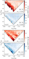 |
Fig. 5. Comparison between the detectability of a variation in Mν and σ8 from the halo 3PCF as a function of triangle shape. We show the results for the simulations at z = 0 with Mν = 0.1 eV and fiducial σ8 = 0.834 (red scale color maps), and with Mν = 0 eV and σ8 = 0.849 (upper blue scale color map) and σ8 = 0.819 (lower blue scale color map). The top and bottom pairs of plots refer to the connected and reduced 3PCF, respectively. Triangle shapes are identified by the side ratios s12/s23 and s13/s23, with s12 ≤ s13 ≤ s23, as shown in Fig. 4. In each plot, a given shape bin shows the absolute value of the detectability, averaged over all triangles available in the all-scales approach with that shape and different sizes. We present the results obtained by considering triangles on scales 30 h−1 Mpc < s23 < 70 h−1 Mpc for ζ, and 70 h−1 Mpc < s23 < 110 h−1 Mpc for Q. |
In ζ, we observe that while the detectability values in the massive-neutrino and variable-σ8 cases are similar in the upper right region of the plots, they differ significantly for elongated triangles (left edge), with the shape-dependent effect induced by massive neutrinos being much more pronounced. In Q, the most evident difference is that the feature produced by massive neutrinos at the location of right-angled triangles is absent for the considered variation in σ8. Furthermore, the shape dependence for folded or near-folded triangles (lower corner) appears different in the two cases. A more quantitative analysis presented in Appendix D shows that at z = 0 for ζ, the average detectability on elongated triangles reaches a ≳7σ discrepancy between massive-neutrino and varying-σ8 simulations, remaining ≲2σ for the other shapes; for Q, the discrepancy is ≳3σ for right-angled and elongated triangles, lying within ∼1σ in the other cases.
Hence, we demonstrate that the three-dimensional shape information of cosmic structures encoded in the 3PCF (unlike the 2PCF, which only captures scale information) is effective in disentangling the effects of massive neutrinos from σ8 rescalings. Our analysis indeed shows that the shape-dependent imprint of massive neutrinos on the 3PCF cannot be replicated by just rescaling σ8, and it identifies the configurations that cause this behavior.
4. Conclusions
We studied the effect of massive neutrinos on the halo three-point statistics in configuration space for the first time by using 2000 N-body simulations from the QUIJOTE suite (Villaescusa-Navarro et al. 2020). We considered simulations at redshifts z = 0, 1, and 2, characterized by values of the sum of neutrino masses Mν = 0.0, 0.1, 0.2, and 0.4 eV.
We estimated the isotropic connected 3PCF ζ and the reduced 3PCF Q (Eq. 3), and we made all the measurements publicly available. To estimate the latter, we also measured the halo 2PCF of our simulations. We ran our measurements with the code MeasCorr (Farina et al. 2026), probing a wide range of scales, from 1 to 150 h−1 Mpc for the 2PCF and from 5 to 145 h−1 Mpc for the 3PCF, thanks to the implementation of the Slepian & Eisenstein (2015a) SHD estimator. We numerically estimated the covariance matrices of the considered statistics from an additional set of 2000 ΛCDM simulations from the QUIJOTE suite itself.
We developed a framework to quantify the neutrino signal in comparison with the fiducial massless case by introducing detectability metrics depending on single and multiple configurations, and on their correlation. We applied this framework to determine the neutrino detectability in a volume of 10 h−3 Gpc3 representative of an ideal redshift bin of a stage-IV survey by rescaling the estimated covariance.
We also used our framework to study whether ζ and Q can provide distinct features that allow us to break the degeneracy between Mν and σ8 that affects two-point statistics. To do this, we complemented our previous dataset (in which σ8 was fixed at the fiducial value 0.834) with measurements performed on three sets of 500 QUIJOTE massless neutrino simulations each, with σ8 = 0.819, 0.834, and 0.849. The main results of our analysis are listed below.
-
For ζ, we found that the effect of neutrinos is stronger for isosceles triangles below ∼30 h−1 Mpc and for quasi-isosceles and squeezed triangles. For Q, we observe a maximum for isosceles triangles, with detectabilities overall lower than for ζ. In correspondence with these configurations, for increasing Mν, we found that the concavity of ζ as a function of the angle between two fixed sides grows, while Q flattens.
-
The signal from massive neutrinos increases with decreasing scale and redshift, following the evolution of nonlinearities. In particular, it is interesting to note that neutrino masses Mν = 0.4 eV can be detected at a 3σ significance already at intermediate or large triangle scales (above ∼50 h−1 Mpc, with values depending specifically on the configuration), while for Mν = 0.2 eV, the 3σ significance is only reached by pushing the configurations to small nonlinear scales (∼5 − 10 h−1 Mpc), which are currently quite difficult to model.
-
We found that massive neutrinos predominantly affect the filaments of the cosmic web. Although most of the signal is on small scales due to free-streaming, we showed that BAO scales are also affected by their presence, but these effects are largely undetectable within the volume probed by stage-IV surveys.
-
By studying the effect of neutrino masses on triangle shapes, we found in ζ the strongest signal for elongated triangles, confirming that filamentary shapes contain the strongest signal, with a preference for squeezed triangles when larger scales are included. For Q, we found that an additional source of signal with respect to ζ is represented by right-angled triangles.
-
We found that the shape dependence of ζ and Q is affected differently by variations in Mν and σ8. In particular, the main differences were found for elongated triangles in ζ and for elongated and right-angled ones for Q. The average detectability shows discrepancies of ≳7σ on elongated triangles between massive-neutrino and varying-σ8 simulations, while remaining below ≲2σ for other configurations. For Q, right-angled and elongated triangles yield discrepancies of ≳3σ, whereas the remaining shapes are consistent within ∼1σ.
This work showed for the first time in the literature that the 3PCF might be employed as a cosmological tool beyond the standard ΛCDM model, in particular, for probing neutrino masses. The extent to which this potential can be effectively unlocked will significantly depend on the smallest scales that can be accurately modeled, a challenging task due to the increasing effect of nonlinearities. For reference, scales below ∼20 h−1 Mpc are currently excluded from the validity range of perturbative models (e.g., Slepian & Eisenstein 2015b, 2017; Kamalinejad & Slepian 2025; Farina et al. 2026). Moreover, the maximum amount of information from clustering studies can be extracted by jointly analyzing lower- and higher-order statistics, as well as by including different observational probes, for example, CMB. We focused extensively on the 3PCF, with the aim of exploring these approaches in future works.
Our analysis also demonstrated that the reduced 3PCF enables the identification of neutrino-induced signatures in structures that are weakly sensitive to their effect in the connected 3PCF (e.g., right-angled triangles). Moreover, the reduced 3PCF has the advantage that its modeling is independent of σ8. Nevertheless, due to the overall lower detectability of the reduced 3PCF compared to the connected 3PCF, a more synergistic exploitation of the former together with the latter will require cosmological volumes larger than those targeted by current surveys.
This paper is the first of an exploratory research program aimed at quantifying the neutrino information content encoded in the 3PCF. In future analyses, we plan to investigate the full-shape dependence of the 3PCF on cosmological parameters (including the sum of neutrino masses) to quantify its constraining power and combine the information provided by higher-order statistics with two-point statistics in a joint likelihood analysis, to maximize the scientific return from galaxy clustering in view of forthcoming data. In this perspective, this work is directly relevant in preparation of the data releases from stage-IV surveys such as Euclid (Laureijs et al. 2011; Euclid Collaboration: Mellier et al. 2025), DESI (DESI Collaboration 2016), 4MOST (de Jong et al. 2019), and the Nancy Grace Roman Space Telescope (Dore et al. 2019), and its potential will be further enhanced by the even larger volumes covered by future stage-V facilities, such as the proposed Wide-field Spectroscopic Telescope (WST; Mainieri et al. 2024), which aims to map the galaxy distribution up to z ∼ 5.5, providing unprecedented statistics.
Acknowledgments
We thank the referee for the constructive comments, which helped to improve the clarity of our paper. We thank Francisco Antonio Villaescusa-Navarro for supporting the public release of our measurements as part of the QUIJOTE suite data products, and Antonio Farina and Marco Baldi for useful discussions. AL acknowledges the use of computational resources provided by the “Open Physics Hub” cluster at the Department of Physics and Astronomy of the University of Bologna. MM and MG acknowledge the financial contribution from the grant PRIN-MUR 2022 2022NY2ZRS 001 “Optimizing the extraction of cosmological information from Large Scale Structure analysis in view of the next large spectroscopic surveys” supported by Next Generation EU. MM acknowledges support from the grant ASI n. 2024-10-HH.0 “Attività scientifiche per la missione Euclid – fase E”.
References
- Abdul Karim, M., Aguilar, J., Ahlen, S., et al. 2025, Phys. Rev. D, 112, 083515 [Google Scholar]
- Adame, A. G., Aguilar, J., Ahlen, S., et al. 2025, JCAP, 07, 028 [Google Scholar]
- Albrecht, A., Bernstein, G., Cahn, R., et al. 2006, ArXiv e-prints [arXiv:astro-ph/0609591] [Google Scholar]
- Bardeen, J. M., Bond, J. R., Kaiser, N., & Szalay, A. S. 1986, ApJ, 304, 15 [Google Scholar]
- Bernardeau, F., Colombi, S., Gaztañaga, E., & Scoccimarro, R. 2002, Phys. Rep., 367, 1 [Google Scholar]
- Bond, J. R., Efstathiou, G., & Silk, J. 1980, Phys. Rev. Lett., 45, 1980 [NASA ADS] [CrossRef] [Google Scholar]
- Brandbyge, J., Hannestad, S., Haugbølle, T., & Thomsen, B. 2008, JCAP, 08, 020 [Google Scholar]
- Brandbyge, J., Hannestad, S., Haugbølle, T., & Wong, Y. Y. Y. 2010, JCAP, 09, 014 [Google Scholar]
- Castorina, E., Sefusatti, E., Sheth, R. K., Villaescusa-Navarro, F., & Viel, M. 2014, JCAP, 02, 049 [CrossRef] [Google Scholar]
- Castorina, E., Carbone, C., Bel, J., Sefusatti, E., & Dolag, K. 2015, JCAP, 07, 043 [CrossRef] [Google Scholar]
- Celoria, M., & Matarrese, S. 2018, ArXiv e-prints [arXiv:1812.08197] [Google Scholar]
- Cole, S., & Kaiser, N. 1989, MNRAS, 237, 1127 [NASA ADS] [Google Scholar]
- Cowan, G., Cranmer, K., Gross, E., & Vitells, O. 2011, Eur. Phys. J. C, 71, 1554 [NASA ADS] [CrossRef] [Google Scholar]
- Davis, M., Efstathiou, G., Frenk, C. S., & White, S. D. M. 1985, ApJ, 292, 371 [Google Scholar]
- de Carvalho, E., Bernui, A., Xavier, H. S., & Novaes, C. P. 2020, MNRAS, 492, 4469 [NASA ADS] [CrossRef] [Google Scholar]
- de Jong, R. S., Agertz, O., Berbel, A. A., et al. 2019, The Messenger, 175, 3 [NASA ADS] [Google Scholar]
- DESI Collaboration (Aghamousa, A., et al.) 2016, ArXiv e-prints [arXiv:1611.00036] [Google Scholar]
- Desjacques, V., Jeong, D., & Schmidt, F. 2018, Phys. Rep., 733, 1 [Google Scholar]
- Dore, O., Hirata, C., Wang, Y., et al. 2019, BAAS, 51, 341 [Google Scholar]
- Elbers, W., Aviles, A., Noriega, H. E., et al. 2025, Phys. Rev. D, 112, 083513 [Google Scholar]
- Euclid Collaboration (Scaramella, R., et al.) 2022, A&A, 662, A112 [NASA ADS] [CrossRef] [EDP Sciences] [Google Scholar]
- Euclid Collaboration (Mellier, Y., et al.) 2025, A&A, 697, A1 [Google Scholar]
- Euclid Collaboration (Guidi, M., et al.) 2026, A&A, 707, A226 [Google Scholar]
- Fang, X., Eifler, T., & Krause, E. 2020, MNRAS, 497, 2699 [NASA ADS] [CrossRef] [Google Scholar]
- Farina, A., Veropalumbo, A., Branchini, E., & Guidi, M. 2026, JCAP, 02, 028 [Google Scholar]
- Fisher, K. B. 1995, ApJ, 448, 494 [NASA ADS] [CrossRef] [Google Scholar]
- Frieman, J. A., & Gaztanaga, E. 1994, ApJ, 425, 392 [Google Scholar]
- Fry, J. N. 1984, ApJ, 279, 499 [NASA ADS] [CrossRef] [Google Scholar]
- Fry, J. N. 1994, Phys. Rev. Lett., 73, 215 [Google Scholar]
- Fry, J. N., & Gaztanaga, E. 1993, ApJ, 413, 447 [NASA ADS] [CrossRef] [Google Scholar]
- Fukuda, Y., Hayakawa, T., Ichihara, E., et al. 1998, Phys. Rev. Lett., 81, 1562 [Google Scholar]
- Gaztañaga, E., Norberg, P., Baugh, C. M., & Croton, D. J. 2005, MNRAS, 364, 620 [Google Scholar]
- Gaztañaga, E., Cabré, A., Castander, F., Crocce, M., & Fosalba, P. 2009, MNRAS, 399, 801 [Google Scholar]
- Grieb, J. N., Sánchez, A. G., Salazar-Albornoz, S., et al. 2017, MNRAS, 467, 2085 [NASA ADS] [Google Scholar]
- Groth, E. J., & Peebles, P. J. E. 1977, ApJ, 217, 385 [NASA ADS] [CrossRef] [Google Scholar]
- Guidi, M., Veropalumbo, A., Branchini, E., Eggemeier, A., & Carbone, C. 2023, JCAP, 08, 066 [Google Scholar]
- Hahn, C., & Villaescusa-Navarro, F. 2021, JCAP, 04, 029 [Google Scholar]
- Hahn, C., Villaescusa-Navarro, F., Castorina, E., & Scoccimarro, R. 2020, JCAP, 03, 040 [CrossRef] [Google Scholar]
- Hamilton, A. J. S. 1992, ApJ, 385, L5 [NASA ADS] [CrossRef] [Google Scholar]
- Hartlap, J., Simon, P., & Schneider, P. 2007, A&A, 464, 399 [NASA ADS] [CrossRef] [EDP Sciences] [Google Scholar]
- Hivon, E., Bouchet, F. R., Colombi, S., & Juszkiewicz, R. 1995, A&A, 298, 643 [Google Scholar]
- Hu, W., Eisenstein, D. J., & Tegmark, M. 1998, Phys. Rev. Lett., 80, 5255 [NASA ADS] [CrossRef] [Google Scholar]
- Ivanov, M. M., Simonović, M., & Zaldarriaga, M. 2020, Phys. Rev. D, 101, 083504 [NASA ADS] [CrossRef] [Google Scholar]
- Jing, Y. P., & Börner, G. 2004, ApJ, 607, 140 [Google Scholar]
- Jing, Y. P., Borner, G., & Valdarnini, R. 1995, MNRAS, 277, 630 [Google Scholar]
- Kaiser, N. 1984, ApJ, 284, L9 [NASA ADS] [CrossRef] [Google Scholar]
- Kaiser, N. 1987, MNRAS, 227, 1 [Google Scholar]
- Kamalinejad, F., & Slepian, Z. 2025, Phys. Rev. D, 112, 083501 [Google Scholar]
- Kamalinejad, F., & Slepian, Z. 2026, Phys. Rev. D, in press [arXiv:2508.06759] [Google Scholar]
- Landy, S. D., & Szalay, A. S. 1993, ApJ, 412, 64 [Google Scholar]
- Laureijs, R., Amiaux, J., Arduini, S., et al. 2011, ArXiv e-prints [arXiv:1110.3193] [Google Scholar]
- Lesgourgues, J., & Pastor, S. 2006, Phys. Rep., 429, 307 [Google Scholar]
- Lesgourgues, J., Mangano, G., Miele, G., & Pastor, S. 2013, Neutrino Cosmology (Cambridge University Press) [Google Scholar]
- Mainieri, V., Anderson, R. I., Brinchmann, J., et al. 2024, ArXiv e-prints [arXiv:2403.05398] [Google Scholar]
- Marín, F. A., Blake, C., Poole, G. B., et al. 2013, MNRAS, 432, 2654 [Google Scholar]
- Marulli, F., Carbone, C., Viel, M., Moscardini, L., & Cimatti, A. 2011, MNRAS, 418, 346 [NASA ADS] [CrossRef] [Google Scholar]
- McBride, C. K., Connolly, A. J., Gardner, J. P., et al. 2011, ApJ, 739, 85 [Google Scholar]
- Meerburg, P. D., Green, D., Flauger, R., et al. 2019, BAAS, 51, 107 [NASA ADS] [Google Scholar]
- Mo, H. J., & White, S. D. M. 1996, MNRAS, 282, 347 [Google Scholar]
- Moresco, M., Marulli, F., Baldi, M., Moscardini, L., & Cimatti, A. 2014, MNRAS, 443, 2874 [Google Scholar]
- Moresco, M., Veropalumbo, A., Marulli, F., Moscardini, L., & Cimatti, A. 2021, ApJ, 919, 144 [NASA ADS] [CrossRef] [Google Scholar]
- Moretti, C., Tsedrik, M., Carrilho, P., & Pourtsidou, A. 2023, JCAP, 12, 025 [Google Scholar]
- Nadal-Matosas, A., Gil-Marín, H., & Verde, L. 2025, JCAP, 01, 045 [Google Scholar]
- Navas, S., Amsler, C., Gutsche, T., et al. 2024, Phys. Rev. D, 110, 030001 [CrossRef] [Google Scholar]
- Oddo, A., Rizzo, F., Sefusatti, E., Porciani, C., & Monaco, P. 2021, JCAP, 11, 038 [CrossRef] [Google Scholar]
- Pardede, K., Rizzo, F., Biagetti, M., et al. 2022, JCAP, 10, 066 [Google Scholar]
- Parimbelli, G., Anselmi, S., Viel, M., et al. 2021, JCAP, 01, 009 [Google Scholar]
- Peebles, P. J. E. 1973, ApJ, 185, 413 [Google Scholar]
- Peebles, P. J. E. 1980, The Large-Scale Structure of the Universe (Princeton University Press) [Google Scholar]
- Peebles, P. J. E., & Groth, E. J. 1975, ApJ, 196, 1 [NASA ADS] [CrossRef] [Google Scholar]
- Peloso, M., Pietroni, M., Viel, M., & Villaescusa-Navarro, F. 2015, JCAP, 07, 001 [Google Scholar]
- Philcox, O. H. E. 2021, Phys. Rev. D, 104, 123529 [NASA ADS] [CrossRef] [Google Scholar]
- Planck Collaboration VI. 2020, A&A, 641, A6 [NASA ADS] [CrossRef] [EDP Sciences] [Google Scholar]
- Pugno, A., Eggemeier, A., Porciani, C., & Kuruvilla, J. 2025, JCAP, 01, 075 [Google Scholar]
- Ruggeri, R., Castorina, E., Carbone, C., & Sefusatti, E. 2018, JCAP, 03, 003 [CrossRef] [Google Scholar]
- Sánchez, A. G., Montesano, F., Kazin, E. A., et al. 2014, MNRAS, 440, 2692 [CrossRef] [Google Scholar]
- Sánchez, A. G., Scoccimarro, R., Crocce, M., et al. 2017, MNRAS, 464, 1640 [Google Scholar]
- Scoccimarro, R. 2004, Phys. Rev. D, 70, 083007 [Google Scholar]
- Scoccimarro, R., Couchman, H. M. P., & Frieman, J. A. 1999, ApJ, 517, 531 [NASA ADS] [CrossRef] [Google Scholar]
- Sefusatti, E., Crocce, M., Pueblas, S., & Scoccimarro, R. 2006, Phys. Rev. D, 74, 023522 [NASA ADS] [CrossRef] [Google Scholar]
- Semenaite, A., Sánchez, A. G., Pezzotta, A., et al. 2023, MNRAS, 521, 5013 [NASA ADS] [CrossRef] [Google Scholar]
- Sheth, R. K., & Tormen, G. 1999, MNRAS, 308, 119 [Google Scholar]
- Slepian, Z., & Eisenstein, D. J. 2015a, MNRAS, 454, 4142 [NASA ADS] [CrossRef] [Google Scholar]
- Slepian, Z., & Eisenstein, D. J. 2015b, MNRAS, 448, 9 [Google Scholar]
- Slepian, Z., & Eisenstein, D. J. 2017, MNRAS, 469, 2059 [Google Scholar]
- Slepian, Z., & Eisenstein, D. J. 2018, MNRAS, 478, 1468 [Google Scholar]
- Slepian, Z., Eisenstein, D. J., Beutler, F., et al. 2017a, MNRAS, 468, 1070 [Google Scholar]
- Slepian, Z., Eisenstein, D. J., Brownstein, J. R., et al. 2017b, MNRAS, 469, 1738 [Google Scholar]
- Slepian, Z., Eisenstein, D. J., Blazek, J. A., et al. 2018, MNRAS, 474, 2109 [Google Scholar]
- Springel, V., White, S. D. M., Jenkins, A., et al. 2005, Nature, 435, 629 [Google Scholar]
- Sugiyama, N. S., Saito, S., Beutler, F., & Seo, H.-J. 2021, MNRAS, 501, 2862 [Google Scholar]
- Szapudi, I. 2004, ApJ, 605, L89 [Google Scholar]
- Szapudi, I., & Szalay, A. S. 1998, ApJ, 494, L41 [NASA ADS] [CrossRef] [Google Scholar]
- Takahashi, T. 2014, Prog. Theor. Exp. Phys., 2014, 06B105 [Google Scholar]
- Taruya, A., Nishimichi, T., & Saito, S. 2010, Phys. Rev. D, 82, 063522 [NASA ADS] [CrossRef] [Google Scholar]
- Umeh, O. 2021, JCAP, 05, 035 [Google Scholar]
- Verde, L., Wang, L., Heavens, A. F., & Kamionkowski, M. 2000, MNRAS, 313, 141 [Google Scholar]
- Verdiani, F., Bellini, E., Moretti, C., et al. 2025, Phys. Rev. D, 112, 043545 [Google Scholar]
- Veropalumbo, A., Sáez Casares, I., Branchini, E., et al. 2021, MNRAS, 507, 1184 [Google Scholar]
- Veropalumbo, A., Binetti, A., Branchini, E., et al. 2022, JCAP, 09, 033 [Google Scholar]
- Viel, M., Haehnelt, M. G., & Springel, V. 2010, JCAP, 06, 015 [CrossRef] [Google Scholar]
- Vielzeuf, P., Calabrese, M., Carbone, C., Fabbian, G., & Baccigalupi, C. 2023, JCAP, 08, 010 [Google Scholar]
- Villaescusa-Navarro, F., Marulli, F., Viel, M., et al. 2014, JCAP, 03, 011 [NASA ADS] [CrossRef] [Google Scholar]
- Villaescusa-Navarro, F., Banerjee, A., Dalal, N., et al. 2018, ApJ, 861, 53 [NASA ADS] [CrossRef] [Google Scholar]
- Villaescusa-Navarro, F., Hahn, C., Massara, E., et al. 2020, ApJS, 250, 2 [CrossRef] [Google Scholar]
- Zel’dovich, Y. B. 1970, A&A, 5, 84 [NASA ADS] [Google Scholar]
At linear order and neglecting nonlocal effects, the perturbative relation between the halo density contrast field δh and the underlying matter density contrast δm can be written as δh = b1δm, where the coefficient b1 is called linear bias (Kaiser 1984; Bardeen et al. 1986; Cole & Kaiser 1989; Mo & White 1996; Sheth & Tormen 1999; Desjacques et al. 2018). The amplitude of the reduced 3PCF of the halos scales with the linear bias b1 as 1/b1 (see Eq. 13 in Gaztañaga et al. 2009).
Appendix A: Neutrino detectability in the 3PCF multipoles
We studied how massive neutrinos affect the multipoles of the connected 3PCF by comparing the detectability of different neutrino masses with the massless case. To avoid repetition, we do not show the analysis for all the possible combinations of redshifts and neutrino masses, but we plot in Fig. A.1 the results obtained for Mν = 0.4 eV at z = 0 as a representative case. We show the detectabilities through a 2D colormap for each multipole ℓ (in the measured range 0 ≤ ℓ ≤ 10), where a given pixel corresponds to a binned triangle side pair (s12, s13).
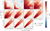 |
Fig. A.1. Detectabilities of neutrino masses (computed with Eq. 10) for the multipoles of the connected 3PCF ζℓ(s12, s13). This figure shows the results for the case of Mν = 0.4 eV at z = 0. |
The fact that neutrinos mostly affect small, nonlinear scales is evident by inspecting the figure, where the highest, positive values of detectability are mostly concentrated on small scales for all the measured ℓ. For ℓ = 0, whose corresponding monopole ζ0 only contributes to the offset of ζ, squeezed triangles (corresponding to the regions adjacent to the bottom and left sides of each colormap, far from the bottom-left corner) also show a positive detectability, decreasing for increasing scale.
The monopole ℓ = 0 and the dipole ℓ = 1 change their sign, exhibiting a mildly negative detectability (for which, in both cases −1 < DET < 0), on a large region of the explored (s12, s13) area. For ℓ = 0, this feature is mostly located along the diagonal region (i.e., for isosceles triangles), divided into two features with 50 h−1 Mpc ≲ s12 ≲ 95 h−1 Mpc and s12 ≳ 105 h−1 Mpc, separated across BAO scales. For ℓ = 1, it shows a fork-shaped pattern, made of three features, one located on the diagonal on scales s12 ≳ 40 h−1 Mpc, and the other ones on scales s12 ≳ 25 h−1 Mpc when 115 h−1 Mpc ≲ s13 ≲ 135 h−1 Mpc and analogously with s12 and s13 interchanged. In the latter two cases, the change in sign observed at fixed s13 ∼ 105 h−1 Mpc (or equivalently at fixed s12 ∼ 105 h−1 Mpc) is driven by the effect of the BAO on the dipole, as shown by the model of Slepian & Eisenstein (2017). This multipole is sourced by the gradient of the density field; therefore, it exhibits a zero crossing at BAO scales, since the acoustic feature corresponds to local maxima in the density distribution.
The multipole that, in the presence of massive neutrinos, shows the most significant departures from the fiducial cosmology is the quadrupole ζ2, which imprints the characteristic parabolic shape to ζ as a function of the angle between two fixed sides, as evident in Fig. 2. For ζ2, on scales s12, s13 ≲ 25 h−1 Mpc the detectability for Mν = 0.4 eV is around 8 and for squeezed configurations it remains ≳2 even for the largest scales probed in our measurement, vanishing only for triangles with large s12 and s13. Starting from ℓ = 3, the highest-detectability pattern progressively concentrates on quasi-isosceles configurations, decreasing with increasing s12 and s13.
Interestingly, for isosceles configurations and ℓ ≥ 2, the detectability patterns show a local minimum. We find that this drop is driven by a local maximum in the standard deviations of all multipoles. Although this maximum is also present for ℓ = 0 and ℓ = 1, the complex detectability pattern of these two multipoles prevents it from being evident in the first two panels of Fig. A.1. Our analysis suggests that this feature originates from autocorrelation within the same radial bin, which occurs for the 3PCF multipoles of isosceles triangles estimated with the Slepian & Eisenstein (2015a) algorithm, as in our case. In the presence of autocorrelation, the expected variance is larger than in the case of cross-correlation between two different radial bins.
Appendix B: Single-scale analysis for the reduced 3PCF
In Fig. B.1 we show the values of the parameter  (Eq. 11) for the reduced 3PCF, computed for the largest neutrino mass Mν = 0.4 eV at redshifts z = 0, 1, and 2. We exclude all the configurations (s12, s13) for which the third side s23 can cross the value 110 h−1 Mpc, to avoid singularities of Q.
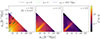 |
Fig. B.1. Same as Fig. 1 but for the reduced 3PCF Q. The white region in each panel corresponds to the configurations excluded by the constraint s12 + s13 ≤ 110 h−1 Mpc. The lines are the same as those overplotted in Fig. 1, for easier comparison with ζ. The (s12, s13) configurations marked with a numbered circle correspond, in increasing order from 1 to 4, to (s12, s13) = (10, 50),(10, 100),(30, 50), and (25, 75) h−1 Mpc. The single-scale Q for these scales is plotted in Fig. B.2. |
The imprint of neutrinos is mainly concentrated in the (s12, s13) bins located along the diagonal, and in the two adjacent ones. The values of  decrease with increasing distance from the diagonal region. Similarly to ζ, the signal increases going to small scales and for decreasing redshift.
For consistency with Fig. 2, we show on the figure the same lines marking the locations of the isosceles, squeezed, and quasi-isosceles configurations with η = 4.
Consistent with the applied scale cut, we select specific configurations, corresponding to (s12, s13) = (10, 50),(10, 100),(30, 50), and (25, 75) h−1 Mpc along and off these lines (for comparison) to inspect the angular behavior of Q visually. We show the corresponding reduced 3PCFs as a function of the third side s23 for all the values of Mν at z = 0, and their associated detectability with respect to Mν = 0 eV, in Fig. B.2.
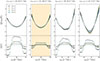 |
Fig. B.2. Single-scale reduced 3PCF Q (upper plot of each panel) for the (s12, s13) configurations selected in Fig. B.1 and indicated at the top, as a function of the third side s23. We show here the results for z = 0, with a different color for each of the considered neutrino masses, as shown in the legend. The lower plots show the corresponding detectabilities as a function of s23 (Eq. 10), with the same color coding as Q. A blue dashed line marks the zero detectability level. The orange shaded area shows the region 90 h−1 Mpc ≤ s23 ≤ 110 h−1 Mpc, corresponding to the expected location of the BAO peak. |
As anticipated in Sect. 2.1, the order of magnitude of Q does not change when varying the configurations (s12, s13) and remains approximately of order unity, unlike ζ in Fig. 2, which instead varies by about one order of magnitude across the selected scales and decreases with increasing scale. The concavity of Q decreases as Mν increases, causing a slight flattening of the function with respect to the measurements for the fiducial massless cosmology. This flattening is reflected in the detectability profile, producing s23-dependent trends with a facing-down concavity: the detectability becomes negative for filamentary structures, i.e., at the edges of the s23 range, and positive for central values. These configurations are the most affected by neutrinos, as they exhibit the largest absolute detectability values. In particular, note that the detectability at intermediate configurations remains relatively stable, with a magnitude comparable to that at the extremes. The flattening of Q with increasing Mν also causes each function measured in the massive-neutrino simulations to intersect the corresponding massless curve at two points, driving the detectability to zero. By inspecting the detectabilities in Fig. B.2, this occurs, regardless of the value of Mν, just below ∼1/4 and just above ∼3/4 of the s23 range.
Due to our scale cut, we do not identify any BAO feature in Q. This occurs because the s23 range is entirely dominated by BAO scales. This is clearly shown in Fig. B.2, where the orange shaded area, corresponding to the expected location of possible BAO features, spans the entire s23 range for (s12, s13) = (10, 100) h−1 Mpc. This implies that any potential BAO signal is spread over the entire range of s23 values, and therefore does not appear as a visible, localized peak.
Appendix C: Scale dependence of the neutrino signal for the reduced 3PCF
We assessed for Q, as we did for ζ in Sect. 3.2, the significance of the massive-neutrino signal relative to the fiducial cosmology as a function of scale, for specific configurations. To do so, we applied the same procedure detailed in Sect. 3.2 to the  values of the configurations (s12, s13) along the lines shown in Fig. B.1.
Figure C.1 shows the scales scross (already defined in Eq. 14) on which the statistical significance of the signal produced by a given neutrino mass Mν at a given redshift becomes higher, when moving from large to small scales, than 1σ and 3σ significance. We follow the same convention of Fig. 3, by setting in Eq. (14) s = s12 for isosceles and quasi-isosceles configurations with η = 4 (being s13 given by, respectively, s13 = s12 and s13 = s12 + 4 × Δsh−1 Mpc), and s = s13 for triangles with s12 = 10 h−1 Mpc.
Since, as visible in Fig. B.1, the signal increases moving toward smaller scales while remaining globally weaker than in the case of ζ, the scales at which it reaches a given significance are smaller for Q than for ζ. This is evident by directly comparing the values of scross for each matrix element in Fig. C.1 with respect to Fig. 3. This implies that cosmological volumes larger than 10 h−3 Gpc3 are required for Q to achieve detectability levels comparable to those shown for ζ.
The figure also shows that restricting the analysis to scales below 110 h−1 Mpc, i.e., those considered for Q in our study, excludes only a negligible fraction of the neutrino signal in a volume of 10 h−3 Gpc3, given that Fig. C.1 indicates that the bulk of the signal is located below 50 h−1 Mpc (there are no printed values of scross exceeding this threshold). Specifically, only the masses Mν = 0.2 eV and 0.4 eV are detectable above 1σ. In particular, cosmic neutrinos with a total mass of Mν = 0.2 eV are detectable above 1σ only at z = 0 (but never above 3σ) for isosceles configurations and for s12 = 10 h−1 Mpc, up to scales of ∼6 h−1 Mpc and 16 h−1 Mpc, respectively. The mass Mν = 0.4 eV is detectable above 1σ at all redshifts only for η = 0, and at z = 0 and z = 1 for squeezed and quasi-isosceles configurations. For these redshift values, squeezed and isosceles triangles also exceed the 3σ detectability on scales between ∼15 and 30 h−1 Mpc, while only at z = 0 for scross ∼ 7 h−1 Mpc in the case of quasi-isosceles triangles. At z = 2, the statistical significance never reaches 3σ, regardless of neutrino mass, redshift, and configuration.
Appendix D: Quantifying the information content of different triangle shapes with respect to variations in Mν and σ8
Here, we complement the analysis presented in Sect. 3.4 by quantifying the capability of different triangle shapes to disentangle the effect of variations in the neutrino mass, Mν, and in σ8 on the connected and reduced 3PCF. The triangular plots shown in Fig. 5 indicate that the largest differences are concentrated in regions of the (s12/s23, s13/s23) plane that lie approximately parallel to the left side of the triangular domain (elongated or right-angled triangles). For this reason, we investigated the detectability in the two different sets of simulations by estimating the average |DET| along directions parallel to the left oblique side, which therefore is expected to provide a more informative way to probe shape-dependent effects.
To this end, we divide our diagram into bins of different shapes (from equilateral to squeezed), which we call “shape index”, as shown in Fig. D.1. We assign a shape index value of 0 to the top-right bin, which contains equilateral triangles, and increase the shape index towards the left side, which corresponds to a value of 20 for the binning adopted in this work.
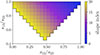 |
Fig. D.1. Legend illustrating the definition of the “shape index” adopted in our analysis for Fig. D.2. A given shape index groups all shape bins lying along a line parallel to the left oblique side, increasing from the top-right corner (equilateral triangles) towards the left side (elongated triangles), as indicated in the colorbar. |
For each bin of shape index, we compute the mean and the standard error of the mean of the absolute values of the detectability of the connected and reduced 3PCF, for simulations with massive neutrinos as well as for those with varying σ8. In Fig. D.2, we present the results at z = 0 as a function of the shape index, separating triangle configurations into small (5 h−1 Mpc ≤ s23 ≤ 30 h−1 Mpc), intermediate (30 h−1 Mpc ≤ s23 ≤ 70 h−1 Mpc), and large (70 h−1 Mpc ≤ s23 ≤ s23, max, with s23, max = 145 h−1 Mpc for ζ and 110 h−1 Mpc for Q) scales. In the plot, we also show the position of particular sets of triangles, namely equilateral, right-angled (identified by the shaded region), and squeezed/folded. In performing this analysis, we consider only those values of shape index associated with at least two populated shape bins.
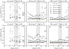 |
Fig. D.2. Mean of the absolute detectabilities (markers) as a function of the shape index (defined in Fig. D.1) at z = 0, for the simulations with massive neutrinos and variable σ8, and its corresponding standard error (error bars). The results for the connected and reduced 3PCF ζ and Q are shown in the top and bottom rows, respectively. Each column corresponds to a different range of triangle scales, depending on the value of the largest triangle side s23, as detailed in the label above each panel: small (5 h−1 Mpc ≤ s23 ≤ 30 h−1 Mpc), intermediate (30 h−1 Mpc ≤ s23 ≤ 70 h−1 Mpc), and large (70 h−1 Mpc ≤ s23 ≤ 145 h−1 Mpc for ζ and 70 h−1 Mpc ≤ s23 ≤ 110 h−1 Mpc for Q). The means are computed only for those shape indices that correspond to at least two populated (s12/s23, s13/s23) bins, depending on the considered scale range and the adopted binning of the side ratios. The schematic representation of triangles in the bottom-right panel qualitatively shows the mapping between the shape index and triangle shapes: low values correspond to equilateral and quasi-equilateral triangles, intermediate values (highlighted by the vertical gray band) to right-angled and quasi-right-angled triangles, and large values to elongated (squeezed/folded) triangles. The vertical axis shows only the mean detectability values below 3, to better highlight the differences between the lowest neutrino mass, Mν = 0.1 eV, and the varying-σ8 simulations. |
On small scales, the trends appear noisier due to the smaller number of triangles averaged, compared to intermediate and large scales (respectively, 43 versus 314 and 2213 for ζ, and 43 versus 314 and 842 for Q). The mean values for the two simulations with varying σ8 are consistent with each other in nearly all values of the shape index, lying on average at ∼0.8σ from each other on intermediate and large scales, and at ∼1.2σ on small scales for ζ (notice, however, that the smaller number of available triangles may significantly influence this last value), and at ∼1σ for Q. In ζ, elongated shapes (high shape indices) dominate the massive neutrino signal at all scales, with a smaller yet noticeable contribution (a factor of ∼4 lower) from intermediate/right-angled configurations at large scales, visible as a small bump at shape index ∼12 for Mν ≥ 0.2 eV. In Q, the bump in the neutrino signal associated with right-angled triangles is clearly visible at intermediate and large scales, and it is only slightly lower than for elongated shapes (a factor of ∼1.5 smaller).
The case Mν = 0.1 eV is particularly relevant for this quantitative analysis, since for this neutrino mass the detectability values are the lowest and comparable to those of the varying-σ8 simulations. On small scales, the signals are difficult to distinguish within the error bars. At intermediate and large scales, for ζ the Mν and σ8 signals start to be significantly distinguishable for more elongated triangles (shape index ∼16); while the mean detectability values remain compatible within ∼2σ at lower shape indices, their differences grow much more rapidly in the massive-neutrino case, reaching discrepancies of ∼10σ and ∼7σ for elongated triangles in the ranges 30 h−1 Mpc ≤ s23 ≤ 70 h−1 Mpc and 70 h−1 Mpc ≤ s23 ≤ 145 h−1 Mpc, respectively. For Q, at intermediate scales the discrepancy is maximal (∼5σ) for shape indices ∼11 − 12, corresponding to right-angled triangle configurations, and gets to ∼3σ for some elongated (shape indices ∼17 − 19) or nearly equilateral configurations (shape indices ∼2 − 4), while remaining ≲1σ for the remaining shapes. At large scales, these discrepancies reach the ∼3σ level for right-angled and elongated triangles and ≲2σ for nearly equilateral ones. We warn the reader that the results for nearly equilateral configurations are based on a limited number of populated bins, as can be easily seen from Fig. D.1, and may therefore be less reliable.
This analysis proves quantitatively, confirming the qualitative indication of Fig. 5, that the imprint of massive neutrinos in ζ and Q across different triangle shapes cannot be reproduced by a simple variation of σ8, since at the same time, some triangle shapes react to this variation similarly to a variation in Mν, while other shapes follow a different trend. This analysis confirms in configuration space the results obtained for the bispectrum in Hahn et al. (2020), paving the way for more systematic studies of the shape-dependent sensitivity of configuration-space higher-order statistics as a promising strategy to disentangle Mν and σ8-related effects.
All Figures
|
Fig. 1. Values of the parameter |
| In the text | |
|
Fig. 2. Single-scale connected 3PCF for the triangle configurations selected in Fig. 1 (upper plots of each panel), as indicated in the top label. We show the results at z = 0, with a different color for each neutrino mass, as indicated in the legend. The inset plots in the upper row show the multipoles ζℓ(s12, s13) from which the 3PCF was reconstructed. The lower plots show the corresponding detectabilities as a function of s23 (Eq. 10). The dashed blue line marks the zero detectability level. The orange shaded areas show the region 90 h−1 Mpc ≤ s23 ≤ 110 h−1 Mpc, corresponding to the expected location of the BAO peak. Where the BAO scales do not cover the full s23 range, we include a zoom-in on the detectability in that region to better visualize the effect of neutrinos in those ranges. |
| In the text | |
|
Fig. 3. Detectability matrices of massive neutrinos. Each matrix element shows the scale scross (Eq. 14) below which, considering all triangles with a scale larger than scross, we obtained a significant detection of the signal from massive neutrinos in the connected 3PCF. The matrices in the upper and lower rows show the values for a 1σ and 3σ statistical significance (Eq. 13), respectively, computed for a volume of 10 h−3 Gpc3. In each matrix, Mν increases from left to right, and redshifts increase from bottom to top. We show the results for the three configurations corresponding to the lines in Fig. 1, i.e., from left to right: triangles with s12 = 10 h−1 Mpc, isosceles triangles (η = 0), and quasi-isosceles triangles with η = 4. The quantity scross represents one of the two sides, s12 or s13, depending on the configuration: in particular, in Eq. (14) we set s = s13 for triangles with fixed s12, and s = s12 for isosceles and η = 4 triangles. Brighter colors represent better detection levels, i.e., occurring at larger scales. The label ND stands for “not detectable” above the specified significance threshold at any scale. A lower limit is indicated whenever the signal is detectable above a given threshold of statistical significance over the entire range of scales considered in our analysis. |
| In the text | |
|
Fig. 4. Detectability of the halo connected 3PCF (upper panels) and reduced 3PCF (lower panels) as a function of the triangle shape. The results are reported at z = 0 and for Mν = 0.4 eV. The triangle shapes are determined by the side ratios s12/s23 and s13/s23, with s12 ≤ s13 ≤ s23. In each panel, each pixel represents a given triangle shape, where the color shows the absolute value of the detectability averaged over all the triangles available in the all-scales approach with that shape and different sizes. As shown in the legend in the upper right panel, the bottom center, upper right, and upper left parts of the plot contain folded, equilateral, and squeezed triangles, respectively. The dotted curve in the lower right panel marks the location of right-angled triangles. The white region corresponds to the area in the parameter space where it is not possible to obtain a closed triangle. The various columns differ by the range of s23 considered, specified in the intervals shown in the bottom right corner (in units of h−1 Mpc). Empty bins are colored in gray. |
| In the text | |
|
Fig. 5. Comparison between the detectability of a variation in Mν and σ8 from the halo 3PCF as a function of triangle shape. We show the results for the simulations at z = 0 with Mν = 0.1 eV and fiducial σ8 = 0.834 (red scale color maps), and with Mν = 0 eV and σ8 = 0.849 (upper blue scale color map) and σ8 = 0.819 (lower blue scale color map). The top and bottom pairs of plots refer to the connected and reduced 3PCF, respectively. Triangle shapes are identified by the side ratios s12/s23 and s13/s23, with s12 ≤ s13 ≤ s23, as shown in Fig. 4. In each plot, a given shape bin shows the absolute value of the detectability, averaged over all triangles available in the all-scales approach with that shape and different sizes. We present the results obtained by considering triangles on scales 30 h−1 Mpc < s23 < 70 h−1 Mpc for ζ, and 70 h−1 Mpc < s23 < 110 h−1 Mpc for Q. |
| In the text | |
|
Fig. A.1. Detectabilities of neutrino masses (computed with Eq. 10) for the multipoles of the connected 3PCF ζℓ(s12, s13). This figure shows the results for the case of Mν = 0.4 eV at z = 0. |
| In the text | |
|
Fig. B.1. Same as Fig. 1 but for the reduced 3PCF Q. The white region in each panel corresponds to the configurations excluded by the constraint s12 + s13 ≤ 110 h−1 Mpc. The lines are the same as those overplotted in Fig. 1, for easier comparison with ζ. The (s12, s13) configurations marked with a numbered circle correspond, in increasing order from 1 to 4, to (s12, s13) = (10, 50),(10, 100),(30, 50), and (25, 75) h−1 Mpc. The single-scale Q for these scales is plotted in Fig. B.2. |
| In the text | |
|
Fig. B.2. Single-scale reduced 3PCF Q (upper plot of each panel) for the (s12, s13) configurations selected in Fig. B.1 and indicated at the top, as a function of the third side s23. We show here the results for z = 0, with a different color for each of the considered neutrino masses, as shown in the legend. The lower plots show the corresponding detectabilities as a function of s23 (Eq. 10), with the same color coding as Q. A blue dashed line marks the zero detectability level. The orange shaded area shows the region 90 h−1 Mpc ≤ s23 ≤ 110 h−1 Mpc, corresponding to the expected location of the BAO peak. |
| In the text | |
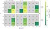 |
Fig. C.1. Same as Fig. 3 but for the reduced 3PCF Q. |
| In the text | |
|
Fig. D.1. Legend illustrating the definition of the “shape index” adopted in our analysis for Fig. D.2. A given shape index groups all shape bins lying along a line parallel to the left oblique side, increasing from the top-right corner (equilateral triangles) towards the left side (elongated triangles), as indicated in the colorbar. |
| In the text | |
|
Fig. D.2. Mean of the absolute detectabilities (markers) as a function of the shape index (defined in Fig. D.1) at z = 0, for the simulations with massive neutrinos and variable σ8, and its corresponding standard error (error bars). The results for the connected and reduced 3PCF ζ and Q are shown in the top and bottom rows, respectively. Each column corresponds to a different range of triangle scales, depending on the value of the largest triangle side s23, as detailed in the label above each panel: small (5 h−1 Mpc ≤ s23 ≤ 30 h−1 Mpc), intermediate (30 h−1 Mpc ≤ s23 ≤ 70 h−1 Mpc), and large (70 h−1 Mpc ≤ s23 ≤ 145 h−1 Mpc for ζ and 70 h−1 Mpc ≤ s23 ≤ 110 h−1 Mpc for Q). The means are computed only for those shape indices that correspond to at least two populated (s12/s23, s13/s23) bins, depending on the considered scale range and the adopted binning of the side ratios. The schematic representation of triangles in the bottom-right panel qualitatively shows the mapping between the shape index and triangle shapes: low values correspond to equilateral and quasi-equilateral triangles, intermediate values (highlighted by the vertical gray band) to right-angled and quasi-right-angled triangles, and large values to elongated (squeezed/folded) triangles. The vertical axis shows only the mean detectability values below 3, to better highlight the differences between the lowest neutrino mass, Mν = 0.1 eV, and the varying-σ8 simulations. |
| In the text | |
Current usage metrics show cumulative count of Article Views (full-text article views including HTML views, PDF and ePub downloads, according to the available data) and Abstracts Views on Vision4Press platform.
Data correspond to usage on the plateform after 2015. The current usage metrics is available 48-96 hours after online publication and is updated daily on week days.
Initial download of the metrics may take a while.