| Issue |
A&A
Volume 708, April 2026
|
|
|---|---|---|
| Article Number | A135 | |
| Number of page(s) | 13 | |
| Section | The Sun and the Heliosphere | |
| DOI | https://doi.org/10.1051/0004-6361/202659037 | |
| Published online | 31 March 2026 | |
The magneto-convective nature of dark striations and moving bright grains at the edge of pores
1
Max-Planck-Institut für Sonnensystemforschung, Justus-von-Liebig-Weg 3, 37077, Göttingen, Germany
2
Thüringer Landessternwarte, Sternwarte 5, 07778, Tautenburg, Germany
3
Big Bear Solar Observatory, New Jersey Institute of Technology, 40386 North Shore Lane, Big Bear City, CA, 92314, USA
4
Center for Solar-Terrestrial Research, New Jersey Institute of Technology, Newark, 07102-1982, NJ, USA
5
Astronomy Program, Department of Physics and Astronomy, Seoul National University, 1 Gwanak-ro, Gwanak-gu, Seoul, 08826, Republic of Korea
6
Korea Astronomy and Space Science Institute, 776 Daedeok-daero, Yuseong-gu, Daejeon, 34055, Republic of Korea
★ Corresponding author: This email address is being protected from spambots. You need JavaScript enabled to view it.
Received:
19
January
2026
Accepted:
28
February
2026
Abstract
Context. High-resolution observations of the Sun reveal a multitude of small-scale striations throughout the photosphere. While these features are well observed in broad-band intensity images, spectropolarimetric observations remain rare.
Aims. In this study, we characterize small dark striations at the pore-granulation boundary and bright grains moving along them. We seek to describe their magneto-convective nature.
Methods. We analyzed restored context images and many-line Stokes inversions of a restored spectropolarimetric scan from GST/FISS-SP with a spatial resolution of 0.068″. In the inversion, we used 85 solar absorption lines within a 33 Å wide spectral window in the 5250 Å region. We compare the observations with a MURaM simulation to discern the magneto-convective nature of striations and grains.
Results. We find multiple dark striations in the vicinity of pores or active region intergranular lanes with a typical width of 0.09″ and moving bright grains that migrate along some of those striations toward the adjacent pore. Grains forming in a high-resolution MURaM simulation of a pore show similar lifetimes of about 70 s. A comparison of the atmospheric configurations of simulated and observed grains reveals good qualitative agreement in structure, dynamics, thermal, and magnetic stratification. The simulation shows that the dark striations form at the top of a convective plume confined by the surrounding field, and that their dark appearance is caused by plasma trapped in the field cusp at optical depth unity. The moving bright grains are composed of hot plasma pulled upwards by turbulent flows at the tip of the striation.
Conclusions. By combining high resolution spectro-polarimetry, many-line inversions, and MURaM simulations, we present the first analysis of the 3D fine structure of small-scale striations and moving bright grains in the vicinity of a pore and describe their magneto-convective nature.
Key words: Sun: magnetic fields / Sun: photosphere / sunspots
© The Authors 2026
 Open Access article, published by EDP Sciences, under the terms of the Creative Commons Attribution License (https://creativecommons.org/licenses/by/4.0), which permits unrestricted use, distribution, and reproduction in any medium, provided the original work is properly cited.
This article is published in open access under the Subscribe to Open model.
Open access funding provided by Max Planck Society.
1. Introduction
Pores are the smaller siblings of the larger and more thoroughly studied sunspots. They exhibit a wide range of sizes and fluxes, spanning from granular scales to small sunspots. Peng et al. (2024) recently presented a statistical comparison between pores and sunspots. The defining difference between sunspots and pores is the penumbra; in its absence, the pore body directly interfaces with granules. The boundary region of pores and surrounding granulation is characterized by small-scale structures such as dark and bright striations, which are typically of the order on or smaller than 0.1 arcseconds in width.
Broadband observations of these features have been reported by various authors, including Scharmer et al. (2002), Lites et al. (2004), Spruit et al. (2010), Schlichenmaier et al. (2016) or Kuridze et al. (2025). Notably, Schlichenmaier et al. (2016) observed that some of these striations form bright grains. By comparing G-band images with simulations, Spruit et al. (2010) described pore-boundary striations as overturning convection similar to penumbral dark lanes. Similarly, Kuridze et al. (2025) compared simulations with observations of striations forming at intergranular lanes and proposed the fluting instability as a driver for their formation. Neither Spruit et al. (2010) nor Kuridze et al. (2025) described the formation of bright grains.
A spectropolarimetric observation of dark striations with a bright grain was reported by Bharti et al. (2016) using the spectropolarimeter aboard the Hinode satellite (HINODE/SP Lites et al. 2001; Kosugi et al. 2007; Tsuneta et al. 2008), but the resolution of HINODE/SP is insufficient to conclusively describe these features. Recently, Zhao et al. (2024) analyzed striations found in an elongated granule. To our knowledge, no other high-resolution spectropolarimetric description that allows extracting information on their stratification has been published to date.
The data from the spectro-polarimetric extension of the Fast Imaging Solar Spectrograph (FISS Chae et al. 2013), referred to as FISS Spectro-Polarimeter (FISS-SP, van Noort et al. 2025), installed at the 1.6 meter clear-aperture Goode Solar Telescope (GST, Goode et al. 2010; Cao et al. 2010; Goode & Cao 2012) at the Big Bear Solar Observatory (BBSO), are currently the only slit-scanning spectrographic data that can reach the diffraction limit in this telescope class and can hence resolve such small-scale features. In this study, we use a time series from the context imager, a many-line inverted (Riethmüller & Solanki 2019; Hölken et al. 2026) spectropolarimetric scan from FISS-SP, and a high-resolution MURaM simulation to investigate the magneto-convective nature of dark striations and moving bright grains.
2. Observation
For this study, we used data from the slit-scanning spectro-polarimeter FISS-SP (van Noort et al. 2025). An emerging active region was observed at μ = 0.81 (cosine of the heliocentric angle) on May 11, 2023, starting from 17:01 (UTC) until 18:48 (UTC). The region was later assigned the NOAA active region (AR) number 13 304, and the central pore developed further into a sunspot in the following days (Munjiba et al. 2024).
The spectropolarimetric scan used here was spatially reconstructed to the diffraction-limited resolution of 0.068″. This reconstruction was performed following the method outlined by van Noort (2017). The data reduction and inversion processes using SPINOR (Frutiger 2000; Frutiger et al. 2000) are described and discussed in detail by Hölken et al. (2026). In the inversion, we made simultaneous use of 85 solar absorption lines within a spectral window of 33 Å in the 5250 Å region. For this study, we used a slightly larger field of view (FOV), as shown in Figure 1, from the same inversion. An overview of the deduced atmosphere is presented in Appendix A.
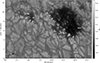 |
Fig. 1. Continuum scan-image constructed from MOMFBD (van Noort et al. 2005) reconstructed slit positions from the FISS-SP context imager. The white arrows indicate striations that formed grains during the observation and indicate the movement direction of the grain. The labels correspond to the panels in Figure 2. The black arrow indicates the direction of the disk center. |
Simultaneously, the region was observed with the FISS-SP context imager. From these broadband intensity images, a 3 arcseconds-wide strip centered on the FISS-SP slit was restored using the multi-object multi-frame blind deconvolution (MOMFBD, van Noort et al. 2005) method, with a final cadence of 2.667 seconds.
3. Simulation
We compared the FISS-SP observation with a magnetohydrodynamic (MHD) simulation of an active region. To produce a model of a small pore, we used the MURaM code (Vögler et al. 2005; Rempel 2017). We employed a multigroup short-characteristics radiation transport scheme including 12 radiation bins, with the bin boundaries outlined by Beeck et al. (2012). The simulation uses the abundances of Asplund et al. (2006); the equation of state is generated using the FreeEoS code (Irwin 2012), and the opacities were calculated using the MPS-ATLAS code (Witzke et al. 2021). The horizontal boundary conditions were periodic. The upper boundary was open to outflows, closed to inflows, and performed a potential field extrapolation into the ghost cells. The lower boundary was open, and allowed passive advection of the magnetic field (OsB of Rempel 2014). To avoid the stringent numerical time-step restriction from the strong magnetic fields, we imposed a limit on the Alfvén speed of 250 km/s using the semi-relativistic Boris correction.
The simulation domain consists of a box with x−, y−, and z-edge lengths of roughly 10 × 10 × 7 Mm, spanning from 4.9 Mm below to 2 Mm above the average τ500 nm = 1 layer. The simulation consists of 1536 × 1536 × 1056 grid points, yielding a regular cubiform voxel grid with an edge length of approximately 6.5 km. The simulation was initiated from a magnetoconvection simulation including only small-scale-dynamo (SSD) fields, similar to those of (Rempel 2014; Przybylski et al. 2025). An additional 400 Gauss uniform vertical field was added to the existing SSD fields, and the simulation was run until the root mean square (RMS) magnetic field in the box saturated. The resolution of this simulation was then increased and run for 15 minutes to allow the small-scale structure to develop. Within these 15 minutes, the evolution was saved every 14.3 seconds, defining the available cadence. Our region of interest in this simulation is the small pore that formed, approximately 2 × 2 Mm in size, which exhibits similar features to the FISS-SP observation.
4. Observational results
In our dataset, we detected several dark striations bordering the pores and strong network intergranular lanes with stronger flux concentrations. The striations are best visible on the limb side. They can have multiple shapes and may appear split or exhibit a snake-like morphology. Some of the striations form bright grains moving alongside or in conjunction with them. Such a grain is a small bright feature at the junction of a split striation or directly attached to the side of a snake-like striation. The intensity of bright grains usually exceeds the intensity of the average quiet Sun (QS). Typical examples of striations and corresponding grains are shown in Figure 2; their apparent movement can be seen in the corresponding animated version. The average full width at half maximum (FWHM) of grain-hosting striations in our dataset is 0.09″. They have an average intensity of about 0.8 IQS, and all of them were found at the borders of the two dominant pores.
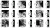 |
Fig. 2. Overview of the nine striations hosting bright grains marked in Figure 1. Each striation is represented by a continuum- intensity image and a TDD. The latter was extracted along the dashed line indicated in the continuum image. The faint dotted line in the TDDs indicates the time of the adjacent context image, and the diagonal dash-dotted green lines track the observed grains in time along the slit. An animated version of this Figure is available as an online movie. |
4.1. Broadband intensity images
In the broadband context images, we frequently observe bright grains appearing on the pore side of the dark striations. From the context images, we selected nine dark striations where the formation, evolution, and decay of a grain was sufficiently sampled. Their location and orientation are indicated with white arrows in Figure 1. We observe two distinct types of these grains. The grains of type Y are bright features between the legs of a Y-shaped striation and the pore, similar to the grains described by Schlichenmaier et al. (2016) and Bharti et al. (2016). The splitting point of the striation and the grain move simultaneously towards the pore. This bound movement gives the impression that the grain is pushed by the striation. In our dataset, the grains A.2, B, C, F, and G (cf., Figure 2 and Table 1) are of this type. In comparison, the grains of type S seem to form as a small bright dot in a strongly curved section at the side of a snake-like striation, which seems to be transported towards the pore by the swaying motion of the striation. Grains A.1, D, and I are of this type. Grain H cannot be conclusively characterized. From our small sample, it appears that S-type grains are generally smaller than their Y-type siblings.
Angular position, horizontal motion, and duration of bright grains.
A scan pass with the restored context images allowed a high-cadence broadband observation of a striation of about 200 s, which is determined by the size of the context image in scan direction and the scan speed1. Figure 2 presents a region of interest (ROI) from a single context image for each grain-forming striation and related time distance diagrams (TDD) that track their temporal evolution along a slit placed parallel to the movement direction. All of the observed grains moved towards their adjacent pore, as shown in the animated version of this figure. In the TDDs, we fit a slope to each grain, indicated as dashed green lines, to estimate the lifetime and apparent horizontal speed of the grains. Table 1 lists the corresponding measured lifetimes and apparent speeds.
To differentiate between limb side and disk-center side striations, we quantified the angle of the track of a grain as the deviation of its apparent movement direction from an idealized straight line pointing towards disk center. With this, the limb-side grains A–G show angles of −20° to 60°, where 0° represents the idealized disk-center direction. The Grains H and I are formed on the disk-center side of the pore and move towards the nearest limb with a relative angle of about 159°. The angles of all grains are given in Table 1. In terms of orientation, Grain F shows an anomaly in the sense that it is not directed towards the largest pore, but to the chain of micro-pores that connect the two larger pores in the dataset.
We did not fully catch the formation of grains A1, D, and E; thus, the mean lifetime of 71.44 s is a lower limit. The mean apparent speed of all these bright grains is about 2.97 km/s. From the context images (see, for instance, animated version of Figure 2), it is clear that most striations that form a bright grain form multiple grains in short succession.
For the two grains on the disk-center side, we find lower speeds and longer lifetimes. The sample sizes of seven and two are too small to allow for a statistical analysis. We speculate that the discrepancy between disk-center and limb-side grains, if not purely statistical, might be due to the difference in viewing angles: When we look along the feature, following the apparent movement direction of the grain into the pore, we also look downwards along the slope of the Wilson depression. This effect can decrease the apparent horizontal speed. We cannot exclude multiple consecutive grains lining up in the line of sight (LOS) either, which would increase the observed lifetime.
4.2. Stratification inferred from the spectro-polarimetric scan
Unfortunately, not all grains visible in the context camera were observed with the spectrograph due to the limited slit coverage and short grain lifetime. The slit covers only one row in the center of the context camera and the average lifetime of a grain is shorter than half of the temporal coverage with the context imager. However, the Grains B, C, and F were sampled with the slit. A cut through the stratified atmosphere, as obtained from the many-line inversions of the polarized FISS-SP spectra, of striation and Grain B is presented in Figure 3, and the other two are shown in Appendix A.
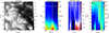 |
Fig. 3. Stratification and context of bright Grain B. Panel (a) presents an FISS-SP integrated-intensity image from the restored scan. The white dashed line indicates the area shown in the other panels. The remaining three panels show cuts through (b) the temperature (T), (c) line-of-sight velocities (vLOS), and (d) field strength (B) stratification. The vertical axis of all three panels represents height in log(τ), indicated left of panel (b). The SPINOR nodes at log(τ) = 0.0, −0.8, and −2.0 are indicated with black, gray, and light gray horizontal lines respectively, and the beginning and end of the grain, based on the continuum image, is marked with white dashed vertical lines in panels b, c, and d, and with a white vertical line in panel (a). In panel (d) the dotted line indicates the azimuth angle, and the dash-dotted line indicates the inclination of the magnetic field corresponding to the y-axis of panel (d). Here, 0° is parallel to the LOS, and the value range is ± 90°. In all figures negative vLOS denotes a flow towards the observer (i.e., up-flow) and positive LOS velocities denote a flow away from the observer (i.e., downflow). |
The observed temperature stratification agrees well with the expectations. We observe a cooler striation and a hotter grain in the lower photosphere, while the upper photospheric temperature seems to be partly determined by the expanding field of the pore.
We found a magnetic canopy with a strongly inclined field spanning from the pore body over the granule (see, Figure 3 panel d). The figure shows the structure as a function of optical depth in log(τ) and distance along the slit. As inversions are performed in optical depth, the canopy-like configuration of the magnetic field does not necessarily correspond to an actual inclination of the field vector. From Stokes Q and we inferred an LOS inclination angle at log(τ) = 0. The extracted mean inclination along this funnel is 72.3° (with 0° parallel to the LOS) and after correction for the angle of incidence (AOI), we obtained ≈53° (with 0° being now parallel to the surface normal). We further observed a secondary magnetic enhancement in the lower log(τ)-layers in the wake of the spectroscopically observed Grains B, C, and F (see also Appendix A). We defer its discussion to Section 5.1, where we compare our observations with a simulation.
This canopy-like field configuration is also observed along striations where we did not resolve the formation of a grain during our observation. A typical example is shown in Figure 4. On close inspection of the inferred atmosphere and corresponding context images, we often found a weak temperature increase in the lower atmosphere and a faint brightening on the side of the striation, but these weak events are too small and hence not conclusively resolved in our dataset. In such quiet striations without resolved grains, we observed a consistent vLOS downflow signature, of typically about 1.5 km/s, over the full length of the feature. In contrast, we observed a structured vLOS pattern in the wake of the grains. All three grains show signatures of a strong upflow following the temperature enhancement in the lower photosphere and a strong downflow in front of it, and they show additional small-scale alternations between upward and downward flows. We found secondary magnetic enhancements and a structured vLOS pattern only in striations that form grains, but in none of the others.
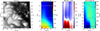 |
Fig. 4. Same as Figure 3 but through an adjacent striation that did not form a grain during observation. |
Cuts perpendicular to the striations, as shown in Figure 5, reveal a clear correlation of the striations with lower temperature, especially in the lower atmospheric layers, but this is visible even in the upper part of the inferred atmospheric model. The vLOS is dominated by a hot downflow, even in the middle of the cut granule. Our dataset shows a ring of hot downflows around all pores, consistent with previous studies (Stein & Nordlund 2000; Bharti et al. 2016). This ring is clearly visible in the low photosphere vLOS maps around all pores in our dataset (see, Hölken et al. 2026, Figure 7 or Appendix A). In Figure 5 this downflow is interrupted with the upflow associated with the grain-forming striation on the left (Grain B, shown in Figure 3) and two regions with weak (up-)flows left and right of the striation on the right (shown in Figure 4).
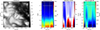 |
Fig. 5. Same as Figure 3 but perpendicular to the striations. We mark the center of the striations based on the intensity image. |
The magnetic field configuration presented in Figure 5 shows roughly the same inclination inside and outside a striation. However, in terms of optical depth, the expanding field from the pore seems to be elevated above the striations. Outside the striations it is detected from log(τ) = −0.8 upwards, while above the striation the canopy field is detected from log(τ) = −1.8 upwards. Whether this is caused by an increased opacity gradient or is a real elevation of the field cannot be conclusively decided from the 3D atmospheric model based on inversions. In the lower nodes, we found the secondary magnetic enhancement in the left striation, as already shown in Figure 3. In the right striation, we found a weak magnetic enhancement, coaligned with the weak upflow just to the right of the striation.
As discussed above, dark striations are not only observed near pores. In our dataset, we also found them next to strong intergranular lanes (IGL) in the plage regions. Figure 6 shows a cut through the stratified atmosphere along such an IGL striation. As in all other cases, we found an expanding magnetic element, that formed in the IGL. The mean AOI-corrected field inclination angle is about 54°, which is similar to the canopy we found at the pore boundary. We did not resolve any grains forming at IGL striations. The downflow pattern in IGL striations is similar to that in pore striations without grain formation (compare, Figure 4). Given these similarities, we infer that striations forming on strong IGLs and on the border of pores are created by the same underlying processes. This motivates a unified interpretation of dark small-scale striations on the intersection of granules and a magnetic element.
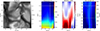 |
Fig. 6. Same as Figure 3 but for a dark striation perpendicular to a dark intergranular lane. Here, the plus in panel (a) and the corresponding white dashed vertical lines in panels (b–d) mark the center of the IGL, based on the intensity image. The location of the striation in the inverted FOV is indicated with a white line marked “IGL” in Figure 1. |
5. Comparison with a MURaM simulation
5.1. Comparability of observation and simulation
In observations we presented, we found that the grains enclosed in the legs of a split dark striation (Y type) or adjacent to a strongly curved striation (S type) are associated with a secondary magnetic enhancement in the lower photosphere. The origin of these field enhancements, which are observed in the wake of the apparent movement direction of the grains, remains unclear from the inferred atmospheric snapshot. Further, the typical swaying, snake-like movement of the dark striations (see the animation of Figure 2) indicates the existence of an instability, for instance fluting and Rayleigh–Taylor instabilities, which could both lead to these type of finger-like structures. To deepen our understanding of the underlying processes, we compared the atmosphere extracted from an observation with a MURaM simulation, shown in Figure 7.
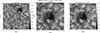 |
Fig. 7. Continuum-intensity snapshot of the MURaM simulation at the optical surface τ500 = 1. Left: Complete simulation domain. Middle: Zoom of the pore. Right: Zoom filtered to a diffraction-limited frame from an ideal 1.6 m telescope. The white rectangles mark the locations of the striations and grains shown in Figures 8 and B.2. |
Our region of interest in this simulation is the small pore with a horizontal extent of about 2 × 2 Mm that shows similar features to the FISS-SP observation: At the boundary of the pore umbra to the granulation in the simulation, we found numerous dark striations forming bright grains. Our FISS-SP observations are restored and the effects of telescope and seeing-induced aberrations have largely been removed. Hence, in order to compare the intensity images from the simulation with those from the observation, we filtered the simulated images, instead of convolving them. We applied a low-pass Fourier filter to remove all structure below the diffraction limit of a 1.6 m telescope. The result of this procedure is shown in the rightmost panel of Figure 7. After filtering, the appearance and evolution of small-scale features around the pore in the simulated intensity images were comparable with the features observed in the FISS-SP context images. Further, the lifetimes of simulated and observed grains were comparable.
Figure 8 shows a cut through the simulated atmosphere of such a grain. Comparing the simulated log(τ)-stratification (last row of Figure 8) with the stratification we extracted from our inverted atmosphere (e.g., Figure 3), we found a good qualitative match of the atmospheric stratification inferred from the observation with the simulated stratification. At log(τ) ∈ [0, −2], simulated and inversion based atmospheres show an increased temperature at the bright feature, a structured up- and downflow pattern, a canopy-like field structure, and a secondary magnetic enhancement in the low photosphere in the wake of the grain.
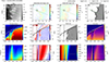 |
Fig. 8. Cut through a grain in a MURaM simulation. Top row: (a) Continuum intensity at 500 nm and the horizontal (b) velocities and (c) field as vector maps, and (d) the vertical field strength, all at log(τ) = 0. All tick marks are in Mm. Middle row: Cuts along the dotted green line indicated in the top row. We plot the temperature (e), vertical velocity (f), vertical field (g) and density (h). All tick marks are in Mm. Bottom row: Vertical cuts through the same quantities as in panels (e)–(h), again along the dotted green line, but with the vertical axis now given in optical depth between log(τ) = 0 and log(τ) = −2, which is similar to the optical depth range covered by the atmospheres obtained from the observations. The tick marks on the x axis are in Mm, tick marks on y axis in log(τ). We adjusted the sign of the vertical flows in all panels to match inversion results, and thus negative values along the z-axis denote an up-flow and positive z-velocities denote a down-flow. The simulated grain is marked with a black circle in panels (a–d) and with a vertical dashed line in panels (e–l). An animated version of this Figure is available as an online movie. |
This similarity persisted for all observed and all simulated events that we investigated. In the simulations, we analyzed four striations forming a total of 14 grains, 11 of which were still visible after filtering to remove structures below the diffraction limit of a 1.6 m telescope. Figure 8 shows an S-type striation that formed a sequence of grains. A Y-type striation with grain is presented in Appendix B. In the simulation, we found that similar processes govern the formation and evolution of both types of striation. Given the agreement of the simulated observables with the actual observations, we conclude that we see the same processes in both. Hence, we used the simulation to discern the formation and evolution of the dark striations and bright grains.
5.2. Formation of the dark striation
Striations occur in weak-field intrusions adjacent to the pore. The physical processes that lead to the appearance of dark striations at the interface between pores and granulation are composed of multiple aspects. The momentum presented in Figure 9 shows that material moves from the forming granule on one side towards the pore on the other side, where it hits the magnetic field, which acts as a boundary.
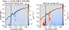 |
Fig. 9. Momentum along the slit indicated in Figure 8a. The vertical dashed line indicates the location of the grain and the black line indicates the log(τ) = 0 surface. Left: Horizontal momentum along the slit. Right: Vertical momentum. The negative horizontal momentum points towards the pore on the left, and negative vertical momentum points upwards. |
Because of the field curvature, the fluting instability, as suggested by Kuridze et al. (2025), is a possible driver for the appearance of the finger-like weak field structure that coincides with the dark striations. However, the pore is almost evacuated and its strong field blocks the denser material flowing towards it from the granule. This behavior might also indicate a convection-driven Rayleigh–Taylor instability (RTI), in which the rapid deceleration of the plasma as it approaches the flux-tube boundary plays the role normally attributed to gravitational force. The field geometry is favorable for an interpretation in terms of fluting instability, but suppression by the strong vertical field (Figure 10) could favor RTI.
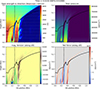 |
Fig. 10. Magnetic field vector, magnetic tension, total pressure and horizontal net force along the slit indicated in Figure 8a. The vertical dashed line indicates the location of the grain, and the black line indicates the log(τ) = 0 surface. The negative horizontal net force points towards the pore. An animated version of this Figure is available as an online movie. |
Cuts perpendicular to the striation, as shown in Figure 11, reveal a different picture. The plume of hot material upwelling underneath the striation indicates a predominantly convective nature of the striations. In this complex situation, it is challenging to disentangle the driving processes, as all of them presumably play a role.
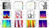 |
Fig. 11. Same as Figure 8, but perpendicular through the grain shown in Figure 8. The black plus in panels (a)–(d) and the vertical dashed lines in panels (e)–(l) mark the center of the striation (based on the intensity). |
While the dominant driver of the striations remains unresolved, their darker appearance can be understood when we analyse the plasma flows. Cuts perpendicular to the striation (Figure 11), show a plume of hot material convecting upwards in the weak field intrusion, elevating the log(τ) = 0 surface. The simulated stratifications show similarities to the signatures that we find in the observations in this case as well (compare Figure 5). At the top, at the log(τ) = 0 surface, the field forms a cusp in which the upflowing material is trapped and then cools due to radiation. This explains the lower temperature, and hence, the darkness of the striations. Similar processes of material trapped in a field cusp have been reported for the dark lanes at the top of umbral dots (Schüssler & Vögler 2006) or for dark lanes in penumbral filaments (Spruit & Scharmer 2006; Spruit et al. 2010; Tiwari et al. 2013) and discussed in Ruiz Cobo & Bellot Rubio (2008). When viewed in geometric height, the cut through the vertical velocities (Figure 11f) shows the convective nature of the striation, with material piling up from below, slowing down, becoming suspended at the top, and then downflowing on the sides.
5.3. Formation of the bright grains
To understand the formation, evolution, and decay of the bright grains, it is best to study the animations of Figures 8 and 10. Along the dark striation, convection pushes nonmagnetic material against the field boundary from the side and from below. The magnetic field forms a funnel (see Figure 8d) that causes the surface flows to accelerate to more than 6 km/s (see Figure 8b). The inwards flow is again decelerated by the magnetic field at the tip of the striation, which is well visible in the net force panel of Figure 10. This destabilization causes turbulent flows (see Figure 8f) wherein hot and cooler material mix, which causes the appearance of the bright and hot grains. The whole evolution is best observed in the animated version of Figure 8.
This process also leads to a steep density gradient, which causes a sharp increase in the optical depth surface. In Figure 8 the steep angle of the log(τ)-surfaces illustrate this nicely. This effect is strongest when observed from a viewing angle that is at near-normal incidence to the slope of the optical depth surface. This explains why we predominantly observe these features on the limb side of the pores. The direction of the flow that causes the grains, from the granule center to its boundary with the pore body, further explains why all observed and simulated grains move inwards towards the umbra.
The secondary magnetic elements in the wake of grains are created by the convection-driven small-scale swirls of the magnetic field (see Figure B.2g). The inwards motion of the plasma and the fast downflows at the head of the striation can amplify these swirls to a detached weak-field intrusion that migrates inwards until its closure (see, the animation of Figures 8d and 8g). This mechanism naturally reproduces the signatures inferred from spectro-polarimetric observations: within log(τ) ∈ [0,−2], the grain corresponds to a localized temperature enhancement cospatial with a structured vLOS pattern of adjacent upflows and downflows.
6. Discussion
The atmospheric stratifications of temperature, vLOS, and magnetic field inferred from a FISS-SP scan match the corresponding stratifications extracted from a MURaM simulation well. At first glance, there appears to be one discrepancy that must be discussed further. While in the observations only some dark striations formed bright grains, in the simulation all dark striations in the vicinity of the pore formed bright grains, sooner or later.
Two mechanisms explain this apparent discrepancy: (i) the observation with the FISS-SP context camera covers 200 s, while the simulation spans roughly 15 min, of which we analyzed the last 10 minutes. In the simulation, grains form almost constantly, but their appearance is scattered over the analyzed 10 minutes. (ii) The restored FISS-SP scans have a resolution of 0.068″, which roughly corresponds to 49 km. The weak temperature and intensity enhancements, as shown in Figure 4, indicate the existence of grains below this resolution limit. In contrast, the simulation has a pixel size of 6 km. Filtering of the simulation to match the spatial resolution of our observations shows that not all simulated grains would be resolved with a 1.6 m telescope. In a randomly selected 200 s sample of filtered simulated intensity images, as shown in the rightmost panel of Figure 7, we found a total of eight grains. The apparent discrepancy can hence be attributed to the missed (in terms of timing) and spatially unresolved formation of grains in some of the striations in the observations.
The similarity of our observations (see Figure 2, especially grains B and F) to the described Y-shaped striations in the granular light bridges reported by Schlichenmaier et al. (2016) and Zhang et al. (2018) is striking. As in our pore scenario, granular light bridges have granulation next to a strong magnetic field, which indicates the similarity of these structures. Such a grain-forming Y-shaped striation was also discussed by Bharti et al. (2016). We further report a new S-shaped grain-forming striation type with a grain forming on the outside of a strongly curved section of the striation.
Other typical dark lanes, such as those reported above umbral dots (Schüssler & Vögler 2006), above filamentary light bridges (Schlichenmaier et al. 2016), or penumbral filaments (Spruit & Scharmer 2006; Zakharov et al. 2008) are formed just below the cusp where two fields of the same polarity merge. Spruit et al. (2010) indeed already indicated a similarity between pore-boundary striations and penumbral filaments and Bharti et al. (2016) reported such a split field above a striation at a pore boundary based on HINODE/SP observations. Our data agree well with these results and the simulation conclusively shows that elevated trapped material in a field cusp at the top of a convective pillar causes the dark appearance, also in the case of the pore-boundary striations discussed here. Zhao et al. (2024) observed striations in an elongated granule associated with a moving magnetic feature (MMF, Harvey & Harvey 1973) and found a rather stable magnetic field configuration over the evolution of different optical appearances. They found a similar magnetic field configuration and strength around and above their striations as we found at the boundary of the investigated pore.
Bharti et al. (2016) and Zhao et al. (2024) connected the striations they studied to formation processes of penumbral filaments. Ruiz Cobo & Bellot Rubio (2008) simulated and discussed differences in the formation of dark lanes in overturning convection and in penumbrae. Munjiba et al. (2024) reported multiple penumbra formations and losses for the AR observed here. However, due to the lack of long-term high-resolution coverage, our dataset does not allow us to speculate about penumbra formation, penumbra model, or similarities between penumbral dark lanes and the striations we observe here.
At first glance, the moving bright grains studied here also seem to be very similar to grains forming in filaments of a developed penumbra (Muller 1973; Zhang & Ichimoto 2013; Tiwari et al. 2013). On closer inspection, we found them to be much smaller, faster, and not as long lived. A further difference is that we only found grains moving inward towards the pore and none moving outward towards the surrounding granulation. Moreover, the general flow direction is only inwards (compare, Figure 8b), and it therefore disagrees with the more complex flow patterns of a developed penumbra (Tiwari et al. 2013). Based on our study, no similarity of these two bright grain types can be established.
The observation we studied was recorded away from the disk center at μ = 0.81. This allowed us to also observe features connected to plage fields, such as strong plage IGLs hosting a magnetic element. The granules close to these IGLs also show dark striations and a cut through the stratification of one example was presented in Figure 6. Considering the similarity of strong plage IGL striations and pore striations (compare Figures 4 and 6) in our dataset, we assume that these plage IGL striations are formed by the same processes as the striations observed at a pore boundary. Kuridze et al. (2025) reported a similar formation process for striations observed in a plage region. The size of the IGL striations from our dataset is at the upper end of the striations studied in their work. This connects our findings to striations on even smaller scales and suggests that the underlying processes driving striation formation are not specific to pores.
7. Conclusion
We have shown that the dark striations and the associated moving bright grains are manifestations of the same magneto-convective process, with plasma trapped and radiatively cooled in a field cusp producing the dark lanes and turbulent tip flows lifting hot material to produce the grains. Further, we offered a physical explanation for the viewing-angle-based selection bias. Our description matches findings from intensity images (e.g., Schlichenmaier et al. 2016; Kuridze et al. 2025) and spectro-polarimetric observations well (e.g., Zhao et al. 2024; Bharti et al. 2016).
Based on the configuration of density, flows, and magnetic field in the simulation, we identified the dark striations as convective features. Multiple instabilities might account for their appearance. Especially, fluting and RTI seem to be likely. The upwelling of hot convection-driven gas might produce the cusp of the field as well, however. The dark appearance of these striations can be explained by trapped plasma in the cusp of the closing magnetic field, similar to dark lanes on umbral dots, penumbral filaments, or filamentary light bridges. The bright grains were identified as fresh material that is mixed upwards by turbulent flows at the tip of the striation. Since this material did not have time to cool, it appears bright.
Based on recent improvements in spectro-polarimetric observations and the availability of high-resolution MHD simulations, we were able to investigate these small-scale features. We analyzed a spectrally and spatially highly resolved spectropolarimetric dataset from GST/FISS-SP (van Noort et al. 2025), inverted with the many-line inversions technique (Riethmüller & Solanki 2019; Hölken et al. 2026) using 85 solar absorption lines. The close match of atmospheric signatures, inferred from the inverted observations, with the atmospheric configuration of a pore in a MURaM-based MHD simulation, enabled us to provide a description of the underlying magneto-convective processes. Our results further establish the good agreement of MURaM simulations with observed solar features.
From nine observed grains (three with spectro-polarimetric coverage), we can report characteristic values for their sizes, lifetimes, and apparent speeds. However, the limited sample and slit coverage motivate further high-resolution spectro-polarimetric observations to test the generality of these results.
Data availability
Movies associated to Figs. 2, 8, 10, and B.2 are available at https://www.aanda.org
Acknowledgments
The contribution of Johannes Hölken was supported by the International Max Planck Research School (IMPRS) for Solar System Science at the University of Göttingen and at TU Braunschweig. The work of J. Chae and J. Kang was supported by the National Research Foundation of Korea (RS-2023-00208117, RS-2023-00273679). BBSO operation is supported by US NSF AGS-2309939 grant and New Jersey Institute of Technology (NJIT). GST operation is partly supported by the Korea Astronomy and Space Science Institute and the Seoul National University. This project has received funding from the European Research Council (ERC) under the European Union’s Horizon 2020 research and innovation programme (grant agreement No. 101097844 – project WINSUN). This study is supported by US NSF grants AGS-2408174, 2401229, 2309939 and NASA grant 80NSSC24K1914. The simulation was conducted using the high performance computing (HPC) clusters at the Max Planck Institute for Solar System research (MPS). For this research we used NASA’s Astrophysics Data System (ADS).
References
- Asplund, M., Grevesse, N., & Jacques Sauval, A. 2006, Nucl. Phys. A, 777, 1 [CrossRef] [Google Scholar]
- Beeck, B., Collet, R., Steffen, M., et al. 2012, A&A, 539, A121 [NASA ADS] [CrossRef] [EDP Sciences] [Google Scholar]
- Bharti, L., Quintero Noda, C., Joshi, C., Rakesh, S., & Pandya, A. 2016, MNRAS, 462, L93 [NASA ADS] [CrossRef] [Google Scholar]
- Cao, W., Gorceix, N., Coulter, R., Coulter, A., & Goode, P. R. 2010, SPIE Conf. Ser., 7733, 773330 [Google Scholar]
- Chae, J., Park, H.-M., Ahn, K., et al. 2013, Sol. Phys., 288, 1 [NASA ADS] [CrossRef] [Google Scholar]
- Frutiger, C. 2000, Ph.D. Thesis, Naturwissenschaften ETH Zürich, Nr. 13896 [Google Scholar]
- Frutiger, C., Solanki, S. K., Fligge, M., & Bruls, J. H. M. J. 2000, A&A, 358, 1109 [NASA ADS] [Google Scholar]
- Goode, P. R., & Cao, W. 2012, SPIE Conf. Ser., 8444, 844403 [NASA ADS] [Google Scholar]
- Goode, P. R., Coulter, R., Gorceix, N., Yurchyshyn, V., & Cao, W. 2010, Astron. Nachr., 331, 620 [NASA ADS] [CrossRef] [Google Scholar]
- Harvey, K., & Harvey, J. 1973, Sol. Phys., 28, 61 [Google Scholar]
- Hölken, J., van Noort, M., Solanki, S., et al. 2026, A&A, 705, A220 [NASA ADS] [CrossRef] [EDP Sciences] [Google Scholar]
- Irwin, A. W. 2012, Astrophysics Source Code Library [record ascl:1211.002] [Google Scholar]
- Kosugi, T., Matsuzaki, K., Sakao, T., et al. 2007, Sol. Phys., 243, 3 [Google Scholar]
- Kuridze, D., Wöger, F., Uitenbroek, H., et al. 2025, ApJ, 985, L23 [Google Scholar]
- Lites, B. W., Elmore, D. F., & Streander, K. V. 2001, ASP Conf. Ser., 236, 33 [NASA ADS] [Google Scholar]
- Lites, B. W., Scharmer, G. B., Berger, T. E., & Title, A. M. 2004, Sol. Phys., 221, 65 [Google Scholar]
- Muller, R. 1973, Sol. Phys., 29, 55 [NASA ADS] [CrossRef] [Google Scholar]
- Munjiba, M. M., Singh, P., Adithya, H. N., Padinhatteeri, S., & Athiray, P. S. 2024, 42nd Meeting of the Astronomical Society of India (ASI), 42, P235 [Google Scholar]
- Peng, Y., Fei, Y., Xiang, N.-B., et al. 2024, ApJ, 975, 23 [Google Scholar]
- Przybylski, D., Cameron, R., Solanki, S. K., et al. 2025, A&A, 703, A148 [NASA ADS] [CrossRef] [EDP Sciences] [Google Scholar]
- Rempel, M. 2014, ApJ, 789, 132 [Google Scholar]
- Rempel, M. 2017, ApJ, 834, 10 [Google Scholar]
- Riethmüller, T. L., & Solanki, S. K. 2019, A&A, 622, A36 [NASA ADS] [CrossRef] [EDP Sciences] [Google Scholar]
- Ruiz Cobo, B., & Bellot Rubio, L. R. 2008, A&A, 488, 749 [NASA ADS] [CrossRef] [EDP Sciences] [Google Scholar]
- Scharmer, G. B., Gudiksen, B. V., Kiselman, D., Löfdahl, M. G., & Rouppe van der Voort, L. H. M. 2002, Nature, 420, 151 [CrossRef] [Google Scholar]
- Schlichenmaier, R., von der Lühe, O., Hoch, S., et al. 2016, A&A, 596, A7 [NASA ADS] [CrossRef] [EDP Sciences] [Google Scholar]
- Schüssler, M., & Vögler, A. 2006, ApJ, 641, L73 [Google Scholar]
- Spruit, H. C., & Scharmer, G. B. 2006, A&A, 447, 343 [NASA ADS] [CrossRef] [EDP Sciences] [Google Scholar]
- Spruit, H. C., Scharmer, G. B., & Löfdahl, M. G. 2010, A&A, 521, A72 [NASA ADS] [CrossRef] [EDP Sciences] [Google Scholar]
- Stein, R. F., & Nordlund, Å. 2000, Sol. Phys., 192, 91 [NASA ADS] [CrossRef] [Google Scholar]
- Tiwari, S. K., van Noort, M., Lagg, A., & Solanki, S. K. 2013, A&A, 557, A25 [NASA ADS] [CrossRef] [EDP Sciences] [Google Scholar]
- Tsuneta, S., Ichimoto, K., Katsukawa, Y., et al. 2008, Sol. Phys., 249, 167 [Google Scholar]
- van Noort, M. 2017, A&A, 608, A76 [NASA ADS] [CrossRef] [EDP Sciences] [Google Scholar]
- van Noort, M., Rouppe Van Der Voort, L., & Löfdahl, M. G. 2005, Sol. Phys., 228, 191 [NASA ADS] [CrossRef] [Google Scholar]
- van Noort, M., Hölken, J., Doerr, H.-P., et al. 2025, A&A, 704, A215 [NASA ADS] [CrossRef] [EDP Sciences] [Google Scholar]
- Vögler, A., Shelyag, S., Schüssler, M., et al. 2005, A&A, 429, 335 [Google Scholar]
- Witzke, V., Shapiro, A. I., Cernetic, M., et al. 2021, A&A, 653, A65 [NASA ADS] [CrossRef] [EDP Sciences] [Google Scholar]
- Zakharov, V., Hirzberger, J., Riethmüller, T. L., Solanki, S. K., & Kobel, P. 2008, A&A, 488, L17 [NASA ADS] [CrossRef] [EDP Sciences] [Google Scholar]
- Zhang, Y., & Ichimoto, K. 2013, A&A, 560, A77 [NASA ADS] [CrossRef] [EDP Sciences] [Google Scholar]
- Zhang, J., Tian, H., Solanki, S. K., et al. 2018, ApJ, 865, 29 [Google Scholar]
- Zhao, J., Yu, F., Zhu, X., et al. 2024, ApJ, 973, 33 [Google Scholar]
To minimize the computational effort we only restored a strip of 3 arcseconds from the context images, that was centered on the FISS-SP slit and moved along with it.
Appendix A: Supplementary figures (inverted observation)
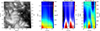 |
Fig. A.1. Same as Figure 3, but for Grain C. The temperature increase in this grain is much more localized as the ones shown in Figures 3 and A.2. The peak is marked with a + in panel (a) and a vertical dashed line in panels (b) to (d). |
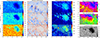 |
Fig. A.3. Maps of the inverted atmosphere similar to Hölken et al. (2026), Figure 7 but with an extended FOV. Here, the lower right panel shows a continuum image. In all figures negative VLOS denote a flow towards the observer (i.e., up-flow) and positive LOS velocities denote a flow away from the observer (i.e., down-flow). Disk-centre is towards the upper right. |
Appendix B: Supplementary figures (simulation)
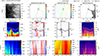 |
Fig. B.1. Same as Figure 11 but cut through the grain shown in Figure 8. The circle in panels (a-d) marks again the grain. |
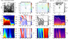 |
Fig. B.2. Same as Figure 8, but for a Y-Type grain. An animated version of this Figure is available as an online movie. |
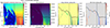 |
Fig. B.3. Same as Figure 10, but for the grain shown in Figure B.2. Please note that the pore is on the right in this plot and hence the positive horizontal horizontal net force is pointing towards the pore. |
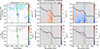 |
Fig. B.4. Momentum along the slit for the grain shown in Figure B.2. Upper row shows the momentum, lower row the non-linear part. Left column shows horizontal parts within the log(τ) = 0-surface, the green line indicates the slit plane with the grain marked by the black circle. Middle column shows horizontal part, projected onto the slit plane, right column the vertical part. The black solid line indicates the log(τ) = 0-surface and the vertical black dashed lines marks the grain position. The positive horizontal momentum is pointing towards the pore on the right and negative vertical momentum is pointing upwards. |
All Tables
All Figures
|
Fig. 1. Continuum scan-image constructed from MOMFBD (van Noort et al. 2005) reconstructed slit positions from the FISS-SP context imager. The white arrows indicate striations that formed grains during the observation and indicate the movement direction of the grain. The labels correspond to the panels in Figure 2. The black arrow indicates the direction of the disk center. |
| In the text | |
|
Fig. 2. Overview of the nine striations hosting bright grains marked in Figure 1. Each striation is represented by a continuum- intensity image and a TDD. The latter was extracted along the dashed line indicated in the continuum image. The faint dotted line in the TDDs indicates the time of the adjacent context image, and the diagonal dash-dotted green lines track the observed grains in time along the slit. An animated version of this Figure is available as an online movie. |
| In the text | |
|
Fig. 3. Stratification and context of bright Grain B. Panel (a) presents an FISS-SP integrated-intensity image from the restored scan. The white dashed line indicates the area shown in the other panels. The remaining three panels show cuts through (b) the temperature (T), (c) line-of-sight velocities (vLOS), and (d) field strength (B) stratification. The vertical axis of all three panels represents height in log(τ), indicated left of panel (b). The SPINOR nodes at log(τ) = 0.0, −0.8, and −2.0 are indicated with black, gray, and light gray horizontal lines respectively, and the beginning and end of the grain, based on the continuum image, is marked with white dashed vertical lines in panels b, c, and d, and with a white vertical line in panel (a). In panel (d) the dotted line indicates the azimuth angle, and the dash-dotted line indicates the inclination of the magnetic field corresponding to the y-axis of panel (d). Here, 0° is parallel to the LOS, and the value range is ± 90°. In all figures negative vLOS denotes a flow towards the observer (i.e., up-flow) and positive LOS velocities denote a flow away from the observer (i.e., downflow). |
| In the text | |
|
Fig. 4. Same as Figure 3 but through an adjacent striation that did not form a grain during observation. |
| In the text | |
|
Fig. 5. Same as Figure 3 but perpendicular to the striations. We mark the center of the striations based on the intensity image. |
| In the text | |
|
Fig. 6. Same as Figure 3 but for a dark striation perpendicular to a dark intergranular lane. Here, the plus in panel (a) and the corresponding white dashed vertical lines in panels (b–d) mark the center of the IGL, based on the intensity image. The location of the striation in the inverted FOV is indicated with a white line marked “IGL” in Figure 1. |
| In the text | |
|
Fig. 7. Continuum-intensity snapshot of the MURaM simulation at the optical surface τ500 = 1. Left: Complete simulation domain. Middle: Zoom of the pore. Right: Zoom filtered to a diffraction-limited frame from an ideal 1.6 m telescope. The white rectangles mark the locations of the striations and grains shown in Figures 8 and B.2. |
| In the text | |
|
Fig. 8. Cut through a grain in a MURaM simulation. Top row: (a) Continuum intensity at 500 nm and the horizontal (b) velocities and (c) field as vector maps, and (d) the vertical field strength, all at log(τ) = 0. All tick marks are in Mm. Middle row: Cuts along the dotted green line indicated in the top row. We plot the temperature (e), vertical velocity (f), vertical field (g) and density (h). All tick marks are in Mm. Bottom row: Vertical cuts through the same quantities as in panels (e)–(h), again along the dotted green line, but with the vertical axis now given in optical depth between log(τ) = 0 and log(τ) = −2, which is similar to the optical depth range covered by the atmospheres obtained from the observations. The tick marks on the x axis are in Mm, tick marks on y axis in log(τ). We adjusted the sign of the vertical flows in all panels to match inversion results, and thus negative values along the z-axis denote an up-flow and positive z-velocities denote a down-flow. The simulated grain is marked with a black circle in panels (a–d) and with a vertical dashed line in panels (e–l). An animated version of this Figure is available as an online movie. |
| In the text | |
|
Fig. 9. Momentum along the slit indicated in Figure 8a. The vertical dashed line indicates the location of the grain and the black line indicates the log(τ) = 0 surface. Left: Horizontal momentum along the slit. Right: Vertical momentum. The negative horizontal momentum points towards the pore on the left, and negative vertical momentum points upwards. |
| In the text | |
|
Fig. 10. Magnetic field vector, magnetic tension, total pressure and horizontal net force along the slit indicated in Figure 8a. The vertical dashed line indicates the location of the grain, and the black line indicates the log(τ) = 0 surface. The negative horizontal net force points towards the pore. An animated version of this Figure is available as an online movie. |
| In the text | |
|
Fig. 11. Same as Figure 8, but perpendicular through the grain shown in Figure 8. The black plus in panels (a)–(d) and the vertical dashed lines in panels (e)–(l) mark the center of the striation (based on the intensity). |
| In the text | |
|
Fig. A.1. Same as Figure 3, but for Grain C. The temperature increase in this grain is much more localized as the ones shown in Figures 3 and A.2. The peak is marked with a + in panel (a) and a vertical dashed line in panels (b) to (d). |
| In the text | |
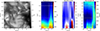 |
Fig. A.2. Same as Figure 3, but for Grain F. |
| In the text | |
|
Fig. A.3. Maps of the inverted atmosphere similar to Hölken et al. (2026), Figure 7 but with an extended FOV. Here, the lower right panel shows a continuum image. In all figures negative VLOS denote a flow towards the observer (i.e., up-flow) and positive LOS velocities denote a flow away from the observer (i.e., down-flow). Disk-centre is towards the upper right. |
| In the text | |
|
Fig. B.1. Same as Figure 11 but cut through the grain shown in Figure 8. The circle in panels (a-d) marks again the grain. |
| In the text | |
|
Fig. B.2. Same as Figure 8, but for a Y-Type grain. An animated version of this Figure is available as an online movie. |
| In the text | |
|
Fig. B.3. Same as Figure 10, but for the grain shown in Figure B.2. Please note that the pore is on the right in this plot and hence the positive horizontal horizontal net force is pointing towards the pore. |
| In the text | |
|
Fig. B.4. Momentum along the slit for the grain shown in Figure B.2. Upper row shows the momentum, lower row the non-linear part. Left column shows horizontal parts within the log(τ) = 0-surface, the green line indicates the slit plane with the grain marked by the black circle. Middle column shows horizontal part, projected onto the slit plane, right column the vertical part. The black solid line indicates the log(τ) = 0-surface and the vertical black dashed lines marks the grain position. The positive horizontal momentum is pointing towards the pore on the right and negative vertical momentum is pointing upwards. |
| In the text | |
Current usage metrics show cumulative count of Article Views (full-text article views including HTML views, PDF and ePub downloads, according to the available data) and Abstracts Views on Vision4Press platform.
Data correspond to usage on the plateform after 2015. The current usage metrics is available 48-96 hours after online publication and is updated daily on week days.
Initial download of the metrics may take a while.