| Issue |
A&A
Volume 709, May 2026
|
|
|---|---|---|
| Article Number | A53 | |
| Number of page(s) | 12 | |
| Section | Interstellar and circumstellar matter | |
| DOI | https://doi.org/10.1051/0004-6361/202557958 | |
| Published online | 30 April 2026 | |
PRODIGE – Envelope to disk with NOEMA
VIII. Sulfur oxides trace a shock caused by a streamer in the inner envelope of a protostar
1
European Southern Observatory,
Karl-Schwarzschild-Strasse 2
85748
Garching bei Munchen, Munchen,
Germany
2
Max-Planck-Institut für extraterrestrische Physik,
Giessenbachstrasse 1,
85748
Garching,
Germany
3
Max-Planck-Institut für Astronomie,
Königstuhl 17,
69117
Heidelberg,
Germany
4
Department of Physics and Astronomy, University of Rochester,
Rochester,
NY
14627-0171,
USA
5
Taiwan Astronomical Research Alliance (TARA),
Taipei,
Taiwan, ROC
6
Institute of Astronomy and Astrophysics, Academia Sinica,
No.1, Sec. 4, Roosevelt Road, Taipei
106319,
Taiwan, ROC
7
Institut de Radioastronomie Millimétrique (IRAM),
300 rue de la Piscine,
38406
Saint-Martin d’Hères,
France
8
IPAG, Université Grenoble Alpes, CNRS,
38000
Grenoble,
France
9
Zentrum für Astronomie der Universität Heidelberg, Institut für Theoretische Astrophysik,
Albert-Ueberle-Str. 2,
69120
Heidelberg,
Germany
10
Centro de Astrobiología (CAB), CSIC-INTA,
Ctra. de Torrejón a Ajalvir km 4,
28806,
Torrejón de Ardoz,
Spain
11
SKA Observatory, Jodrell Bank, Lower Withington,
Macclesfield
SK11 9FT,
UK
12
Laboratoire d’Astrophysique de Bordeaux, Université de Bordeaux, CNRS, B18N, Allée Geoffroy Saint-Hilaire,
33615
Pessac,
France
13
Observatorio Astronómico Nacional (IGN),
Alfonso XII 3,
28014
Madrid,
Spain
14
Université Paris-Saclay, CNRS, Institut d’Astrophysique Spatiale,
91405
Orsay,
France
15
Space Research Institute, Austrian Academy of Sciences,
Schmiedlstr. 6,
8042
Graz,
Austria
★ Corresponding author: This email address is being protected from spambots. You need JavaScript enabled to view it.
Received:
3
November
2025
Accepted:
14
March
2026
Abstract
Context. Recently, streamers have been observed causing shocks at the outer edge of protoplanetary disks. The study of sulfur-bearing species can help us to understand the physical and chemical changes caused by infalling streamers toward their landing positions.
Aims. We study the physical properties traced by the emission of SO2 and SO toward the Class I protostar Per-emb 50, which is possibly related to the streamer infalling toward its disk.
Methods. We present new NOrthern Extended Millimeter Array (NOEMA) A-array observations as part of the large program “Protostars and Disks: Global Evolution” (PRODIGE). We analyzed the morphology of SO2 and SO, and complement our interpretations with additional H2CO and CO data from the same program. We compared the SO2 and SO morphology with an infalling-rotating model. We applied Bayesian model selection to the brightest SO2 line to disentangle the different kinematic components traced by this molecule. We used local thermodynamic equilibrium (LTE) and non-LTE analyses to determine the temperature and density of the SO2 emission.
Results. There are two separate peaks of SO2 emission offset toward the southwest of Per-emb 50: one brighter (peak 1) at about 180 au from the protostar, and a weaker one (peak 2) at about 400 au. Peak 2 is blueshifted with respect to an infalling-rotating envelope. We propose that this peak is caused by the shock between the inner envelope and the streamer. Peak 1 is consistent with the expected envelope motion, and could thus be caused by shocks at the disk-envelope interface, but potential streamer influence cannot be neglected. Both peaks show abundance ratios consistent with a low-velocity shock (~3–4 km s−1) when compared with shock models.
Conclusions. Streamers can affect the physical and chemical structure of both disks and envelopes, suggesting that streamers can play an important role in shaping both structures in the embedded stages of star formation.
Key words: astrochemistry / shock waves / stars: formation / ISM: kinematics and dynamics / ISM: molecules
© The Authors 2026
 Open Access article, published by EDP Sciences, under the terms of the Creative Commons Attribution License (https://creativecommons.org/licenses/by/4.0), which permits unrestricted use, distribution, and reproduction in any medium, provided the original work is properly cited.
This article is published in open access under the Subscribe to Open model. This email address is being protected from spambots. You need JavaScript enabled to view it. to support open access publication.
1 Introduction
The evolution of protostars and their planet-forming disks is fundamental to understanding how planets (such as Earth) are formed. Protostars are part of a complex, dynamic system, with energetic outflows ejecting material and transporting angular momentum, and infalling material feeding the disk simultaneously (Tobin & Sheehan 2024, and references within). These processes can have a deep impact in the physical (e.g., Hennebelle et al. 2017; Zamponi et al. 2021; Kuznetsova et al. 2022; Maureira et al. 2022) and chemical properties of disks (e.g., Sakai et al. 2014; Vastel et al. 2022; Podio et al. 2024; Hsieh et al. 2025b). In particular, the chemical properties of protostellar disks are fundamental to understanding what materials are inherited from the interstellar medium (ISM), and what has been reprocessed within the disk (Pontoppidan et al. 2014; Drozdovskaya et al. 2018; Ceccarelli et al. 2023).
Infall of envelope material causes a shock when entering the disk. This shock heats up the surrounding gas, potentially increasing the temperature to hundreds of Kelvin (Draine et al. 1983; Neufeld & Hollenbach 1994). Thus, shocks can change both the conditions of the material fed to the disk and within the disk itself. Given the hints that planet formation begins in these early, embedded stages (Manara et al. 2018; Tychoniec et al. 2020; Sheehan et al. 2020; Segura-Cox et al. 2020; Hsieh et al. 2025a), investigating how disk and envelope material changes is essential to understanding our chemical inheritance.
Not all infall from the environment comes from a symmetric envelope. Asymmetries in envelopes are common toward low-mass protostars (e.g., Tobin et al. 2012). Recently, streamers have been observed toward a variety of protostars, of different masses and ages, located across different star-forming regions (Pineda et al. 2023; Tobin & Sheehan 2024, and references within). These can bring material from beyond the envelope (Pineda et al. 2020; Valdivia-Mena et al. 2023; Taniguchi et al. 2024; Gieser et al. 2025), expanding the material reservoir available for stellar and planetary growth. In some cases, the streamer’s chemical footprint suggests that the funneled mass is prestellar in nature (Taniguchi et al. 2024; Podio et al. 2024). The study of the effects of streamers onto protostellar (e.g., Flores et al. 2023; Artur de la Villarmois et al. 2022; Aso et al. 2023; Podio et al. 2024; Liu et al. 2025; Kido et al. 2025) and protoplanetary disks (Garufi et al. 2022; Speedie et al. 2025) has been an active area of research in the last few years. It is uncertain if the material brought by streamers can be directly inherited by forming planets or if it is chemically reset due to the impact between them and disks. Therefore, understanding the shock conditions produced by streamers is fundamental to determining the chemical effects of streamers.
Sulfur-bearing molecules are commonly used as tracers of heated regions, such as shock fronts, given their sensitivity to the physical conditions of their environment (Sakai et al. 2014; Oya et al. 2025). In particular, SO and SO2 have been associated with shocks caused by both envelope infall (Sakai et al. 2014) and streamers (Garufi et al. 2022; Speedie et al. 2025), sometimes with both phenomena occurring at the same time (Liu et al. 2025). SO and SO2 emission are sensitive to shock conditions (such as velocity and pre-shock number density, nH) as its formation pathways in the gas phase are closely tied to shock-related processes (e.g., van Gelder et al. 2021). Both species can be sublimated from dust grains in shocks and also formed in the gas phase due to the temperature increase caused by shocks, but SO thermal desorption requires lower velocities and densities than SO2 as its sublimation temperature is lower (37 K for SO versus 62 K for SO2, van Gelder et al. 2021), and thus the former can be more easily detected (Aota et al. 2015). The study of these sulfur-bearing species can then help us understand the conditions of shocks caused by streamers.
In this article, we investigate the emission of the sulfurbearing molecules SO2 and SO toward Per-emb 50, a Class I protostar with a known streamer. Per-emb 50 is located in NGC 1333, an active star-forming region within the Perseus Molecular Cloud, at a distance of 298 pc (Zucker et al. 2018). Previously, Valdivia-Mena et al. (2022) found a streamer toward this source in H2CO 30,3–20,2 emission, with an extension of at least 3300 au in the southwest direction, transporting material from beyond the envelope toward the vicinity of the disk. In the same work, they found an unresolved SO2 emission peak offset from the protostar’s position toward the southwest, and suggested that this was caused by the accretion shock from the streamer material impacting near the disk. Later, data from the Perseus ALMA Chemistry Survey (PEACHES, Zhang et al. 2023) showed that the enhancement of SO and SO2 toward the southwest coincided with a change in the dust properties of the envelope, consistent with an accretion shock. We have obtained new NOEMA observations using the most extended configuration (A), which allows us to investigate the SO2 and SO emission in more detail and find out if the sulfur species’ emission is consistent with a shock caused by the streamer.
This paper is organized as follows. Section 2 presents the new NOEMA data, which is part of the large program “Protostars and Disks: Global Evolution” (PRODIGE). This program has been fruitful for the discovery of streamers toward low-mass protostars (Valdivia-Mena et al. 2022; Hsieh et al. 2023; Gieser et al. 2024, 2025). In Sect. 3, we show the physical properties found through SO2 and SO emission and explain the steps we took to arrive at these results. In Sect. 4, we argue that part of the observed SO2 and SO emission is caused by the streamer producing a shock in the inner envelope of the protostar. A summary of this work is presented in Sect. 5.
2 Observations and data reduction
We used the NOEMA C and D array observations for Per-emb 50 from the PRODIGE Max Planck – IRAM Observing program. Per-emb 50 was observed with C configuration on 29 December 2019 and 5 January 2020. Details of the data reduction are in Valdivia-Mena et al. (2022). In summary, we used the data reduction pipeline available in CLIC within the IRAM servers, and combined the uv tables using uvmerge. The C and D combined data were phase self-calibrated with solution intervals of 30, 135, and 45 s, using the mapping self-calibration module, and then applied the phase solutions to the continuum and line data.
Observations with NOEMA A configuration were taken during 19 and 21 January 2023 under project W22AH (PI: Valdivia Mena). We designed the A observations with the same spectral setup as the PRODIGE observations so that the data could be directly combined. We calibrated the data using the NOEMA pipeline available through the GILDAS CLIC package. We self-calibrated the data using the GILDAS mapping self-calibration module. The iterative self-calibration was performed with solution intervals of 300 s, 135 s, and 66 s on the continuum data, which includes only line-free channels. We applied the phase gain solutions to the continuum and line uv tables.
We combined and imaged the data using the MAPPING package from the GILDAS suite1. We used the self-calibrated uv tables from the PRODIGE data reduction process and the self-calibrated A-configuration uv tables. We combined the A and CD array uv tables using uv_merge. Continuum subtraction was done manually on the combined uv tables using the uv_baseline command.
We imaged the SO, SO2, CO, and H2CO line cubes from the combined arrays’ narrowband units, which have a native resolution of 62.5 kHz (approximately 0.08 km s−1 for the rest frequencies of the investigated lines). We imaged using the classical Hogbom CLEAN algorithm (Högbom 1974) with natural weighting. We manually masked the emission in the deconvolved image to improve the image quality and reduce emission sidelobes. The data cubes have a spatial resolution of approximately 0.8″ × 0.3″, with a position angle (PA) of −0.2 deg. Their properties are summarized in Table 1.
We smoothed all SO2 data cubes to a resolution of 0.21 km s−1 to increase the signal-to-noise ratio (S/N) of SO2 transitions 42,2–31,3 and 123,9–122,10, which are weaker than SO2 111,11–100,10. The cubes after smoothing have a root mean square (rms) of about 0.5 K (Table 1).
We also obtained the continuum emission toward Per-emb 50 from the wideband units. We imaged the continuum using the Hogbom CLEAN algorithm with robust weight (Briggs), with a robust parameter value of 1, and applied manual masking to improve image quality. The continuum is unresolved for the resolution of our data (0.78 × 0.28″, −180.26°) and has an rms of 0.15 mJy beam−1. The location of the protostar used throughout this work is the location of the maximum peak in the continuum image (RA(J2000) = 3h09m07s.77, Dec(J2000) = ![Mathematical equation: $\[+31^{\circ} 21^{\prime} 56^{\prime\prime}_\cdot 99\]$](/articles/aa/full_html/2026/05/aa57958-25/aa57958-25-eq1.png) ).
).
Molecular transitions and their properties.
3 Results and analysis
3.1 Morphology of molecular emission
Figure 1 shows the integrated intensity maps of SO2 and H2CO, together with SO and CO contours. The SO2 peak seen in Valdivia-Mena et al. (2022) is resolved into two separate intensity peaks. They are seen in all SO2 transitions, but most prominently in the brightest SO2 line (111,11–100,10, shown in Fig. 1). Maps of the rest of SO2 transitions are presented in Appendix A. The location of the two SO2 peaks are offset from the position of the continuum emission in the southwest direction. The brightest peak, which we label peak 1, is located ~180 au (0.6″) from the protostar, whereas the second, weaker peak (peak 2) is ~400 au (1.3″) away. There is also weak SO2 emission toward the north of the protostar, seen only in the brightest transition.
The brightness distribution of SO is more extended than SO2, with strong emission (S/N > 5) toward both north and south of the protostar, but the brightest emission both in integrated intensity and in peak brightness temperature (TMB) coincide with SO2 peaks 1 and 2 (Fig. 1 right). Valdivia-Mena et al. (2022) showed that SO emission can be fit with up to three velocity components that trace different structures, included the streamer toward the southwest, but there was only one beam-sized emission peak south of the protostar in the C and D configuration data (beam of 1.2″). Adding the A configuration, this peak resolves into two distinct emission peaks (at a resolution of 0.8″).
H2CO distribution peaks toward the west of the SO2 peak 2 and is extended, reaching approximately the same declination as the protostar. This new data resolves the part of the streamer first seen in Valdivia-Mena et al. (2022) that shows the strongest velocity change, accelerating toward blueshifted velocities with respect to the protostar. There is no SO2 emission at the location of H2CO and vice versa (Appendix A), but there is SO emission at the location of the streamer with the same velocity.
CO traces the outflow cones that are approximately in the east-west direction, as shown in the contours of Fig. 1 right. At this resolution, CO emission is also tracing part of the inner envelope and disk surrounding the protostar, hinted at by the peaks of both redshifted and blueshifted CO located south and north of the protostar, as shown in Appendix A, aligned with the previously known rotation from the envelope and disk (Valdivia-Mena et al. 2022; Zhang et al. 2023). Based on the integrated intensity maps, SO2 peak 1 appears close to the base of the outflow, where CO shows redshifted emission. However, peak 2, farther away, is not associated with high-velocity CO emission.
3.2 Kinematics traced by SO2 and SO
We made position–velocity (PV) diagrams for our SO2 and SO emission cubes along the white line shown in Fig. 1 right (190 deg from north), which corresponds to the envelope PA found in Zhang et al. (2023), to check if our SO2 and SO detected emission traces rotational signatures. We compared the emission in both peaks with an infalling-rotating envelope (IRE) model obtained using the FERIA code (Flat Envelope Model with Rotation and Infall under Angular Momentum Conservation, Oya et al. 2022) to further analyze the kinematics of peaks 1 and 2. We describe how we obtained the IRE model PV diagram in Appendix A. The resulting PV diagrams are in Fig. 2.
Both SO2 and SO transitions show a clear redshifted peak at approximately 9.5 km s−1 in the PV diagrams, which corresponds to peak 1 in the moment 0 map of Fig. 1. This peak is located at the expected position and velocity for the redshifted emission peak of the IRE model described in Zhang et al. (2023). The rest of the emission in that quadrant has lower velocities than those expected from the IRE model. This brightness distribution is associated with peak 2 from the SO2 moment 0 map. There is both redshifted and blueshifted emission within a beam of the protostar with high velocity (up to 5 km s−1 from the vLSR), probably associated with a Keplerian disk around the protostar, seen in all transitions except for SO2 123,9–122,10, the one with highest Eup (93 K). Both molecules show a skewed diamond shape that is an indication of a combination of rotation and infall gas motions.
Figure 3 shows the SO2 and SO spectra at the two peak positions (crosses in Fig. 1) together with the expected line shape for emission corresponding to an IRE. The expected IRE velocity in the envelope at peak 1 coincides with the observed SO and SO2 maxima, whereas for the peak 2, SO2 and SO emission is blueshifted from the expected IRE peak (9.1 km s−1) by approximately 1.4 km s−1. Both molecules’ emission could also include a component of IRE, seen as a redshifted shoulder in the spectra, but the peak of the emission does not correspond to envelope kinematics. For comparison, we label the velocity of the streamer head obtained through the fit of H2CO velocity components (6.45 km s−1; Appendix B). Peak 2 velocity is in between the streamer velocity and the expected IRE velocity at that location.
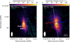 |
Fig. 1 NOEMA observations of molecular emission toward Per-emb 50. Left: integrated intensity of SO2 111,11–100,10 between 6.5 and 12 km s−1. Black crosses show the locations of the SO2 peaks, labeled as peak 1 and peak 2. Cyan contours represent the H2CO 30,3–20,2 integrated intensity between 5 and 8 km s−1, drawn in steps of 3, 5, and 10 times the rms of the integrated image (0.7 K km s−1). Right: integrated intensity of SO 55–44 between 0 and 13 km s−1. The red and cyan contours are the CO integrated intensity in redshifted and blueshifted channels, respectively, with respect to the protostar’s vLSR (7.5 km s−1). Blueshifted channels are integrated between −4.3 and 5.3 km s−1, and redshifted channels between 10 and 20 km s−1. Contours are drawn at 5–45 times the rms of the integrated images (4.7 K km s−1) in steps of 10. Red and blue arrows indicate the direction of the outflow. The dashed line represents the direction of the PV diagram in Fig. 2. The white star marks the position of the continuum peak. The filled white ellipse represents the beam size. A scale bar in the bottom right corner represents a physical scale of 200 au. |
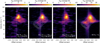 |
Fig. 2 Position velocity diagrams of SO2 and SO using the path shown in Fig. 1. SO2 transitions are in order of increasing upper energy levels, Eup. From left to right: SO2 42,2–31,3, SO2 111,11–100,10, SO2 123,9–122,10, SO 55–44. White contours show the normalized intensity PV diagrams for an IRE, obtained with FERIA (Oya et al. 2022). |
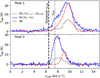 |
Fig. 3 Spectra of SO 55–44 (blue) and SO2 111,11–100,10 (gray) at the two resolved peak positions, together with the spectra obtained from FERIA, normalized to the SO intensity at the peak velocity of the IRE. The vertical dash-dotted line marks the systemic velocity of the protostar (7.5 km s−1), whereas the thick dashed line marks the velocity of the streamer at the same distance from the protostar (in radius) as peak 2 (6.45 km s−1; Appendix B). |
3.3 Separation of individual velocity components
The PV diagrams in Fig. 2 and spectra in Fig. 3 suggest that there is more than one kinematic component traced by S-bearing molecules. To investigate the physical nature of the SO2 peaks, we fit up to three Gaussian velocity components to the SO2 111,11–100,10 spectra in each pixel. We applied Bayesian model selection with the nested sampling parameter exploration algorithm, using the pyspecnest Python package (Sokolov et al. 2020). Details of the application of this method to molecular line observations are given in Sokolov et al. (2020). In summary, the nested sampling algorithm searches for the best parameters for each model – in this case the different models are one, two, and three Gaussian components – and returns the Bayes factor, K, for each pair of models, which we use to select the optimal number of Gaussian components in each pixel. We applied the algorithm to all spectra with S/N> 5, and each pixel was assumed to be independent. Details of this process are in Appendix C.
Figure 4 shows the best Gaussian fits at the locations of the two SO2 peaks. Peak 1 is best fit using two Gaussian components, a wide one (σv ~ 4 km s−1) and a narrow one (σv = 0.7 km s−1), whereas peak 2 is best fit by one narrow Gaussian component, according to our model selection criterion (Appendix C). The Gaussian fit does not capture the skewness shown by peak 2’s line profile, better seen in Fig. 3, but this does not affect our subsequent analysis. The Gaussian components that dominate the flux in both locations have similar velocity dispersions (peak 1 has σv = 0.7 km s−1, and peak 2, σv = 0.8 km s−1).
The fit results indicate that close to the protostar, one of the Gaussian components has a large σv value with respect to the majority of pixels. We determined the σv threshold to separate between narrower and wider Gaussian components close to the protostar by estimating the probability density function (PDF) of the σv distribution. Details of this estimation and the resulting distribution of σv values are in Appendix C (Fig. C.2). The majority of the Gaussian components have σv ≈ 1 km s−1 and there is an inflection point around σv = 1.8 km s−1. We separated the Gaussian component with σv > 1.8 km s−1 (wide) from the rest of the components (narrow) to analyze both separately. In the locations where there are two components with σv < 1.8, we chose the one that had the velocity closest to its neighbors. The velocity patterns when separating both components by σv are in Fig. 5.
The two Gaussian components (narrow and wide) show patterns consistent with rotation, with the northeast side blueshifted with respect to the protostar and the southwest redshifted. Components with σv > 1.8 km s−1 are concentrated around the protostar, in a radius of about 200 au. Their velocity pattern and large velocity dispersion suggest this SO2 component traces a rotating gas disk, consistent with the shape of the PV diagram at that location (Fig. 2). The narrow Gaussian components are more extended in space and include the bright peaks seen in the integrated maps (Fig. 1). These also show a redshifted-blueshifted pattern aligned with the rotation seen in the wide component, consistent with the kinematics of the IRE seen in the PV diagram. Thus, we associate the narrow SO2 component with IRE emission.
The region in between the two SO2 peaks has two narrow Gaussian components according to the nested sampling results (Appendix C). The fit in this region shows a potential bridge in the velocities. However, this region is smaller than one beam size, so we did not analyze this bridge further. We selected in this region the brightest component to show in Fig. 5.
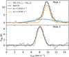 |
Fig. 4 SO2 spectra (gray) at the location of the peaks together with the best-fit (dashed black lines) Gaussian models. Peak 1 has two Gaussian components, a narrow one (orange, σv < 1.8 km s−1) and a wide one (blue, σv > 1.8 km s−1), whereas peak 2 has just one component (narrow). |
3.4 Physical conditions of the SO2 peaks
We estimated the physical conditions traced by all three SO2 transitions (Table 1) for the narrow component found in Sect. 3.3. Separating the disk (wide) from the envelope (narrow component) allows us to determine the densities and temperatures of each peak, avoiding contamination from the disk component. We first assumed local thermodynamic equilibrium (LTE) conditions and then used the line ratios at the location of the peaks to corroborate the obtained column densities without assuming LTE.
We fit the three observed SO2 lines with the eXtended CASA Line Analysis Software Suite (XCLASS, Möller et al. 2017)2, using the myXCLASSfit module in Python. XCLASS fits the spectra of all transitions simultaneously, assuming LTE but not optically thin emission, instead correcting for optical depth effects. We did a pixel-by-pixel LTE fit fixing the number of components, their central velocities, and velocity dispersions to the values obtained from the nested sampling fit (Sect. 3.3), assumed a beam filling fraction of 1, and left the rotational temperature, Trot, and the column density, N(SO2), as free parameters. We only fit pixels where all three transitions show emission with S/N > 5.
The resulting temperature and column density for the narrow SO2 components are shown in Fig. 6. The specific values obtained from the LTE fit at the location of each peak are in Table 2. For the two SO2 peaks, we obtained the uncertainties in temperature and column density by running the Markov chain Monte Carlo (MCMC) algorithm, implemented in the myXCLASSfit module, whereas for the central velocities and FWHM, the uncertainties come from the nested sampling. Both peaks show different physical conditions. The SO2 column density at the peak 1 is about 0.2 dex higher than the column density at peak 2 (which is closer to the streamer), and the temperature of the former is about 20 K higher. The velocity dispersion, however, is similar in both locations (also seen in Fig. 4). The column densities are close to 1015 cm−2, within the range estimated by Artur de la Villarmois et al. (2023) but higher by almost two orders of magnitude than the column densities found in Zhang et al. (2023). In both cases referenced above, the column density was calculated using a non-LTE calculation and only one transition of SO2 was used (140,14–131,13), introducing a high uncertainty. Nevertheless, values around 1015 cm−2 have been reported at distances about 500 au from a protostar, such as in the Elias 29 ridge region (Oya et al. 2019), which is associated with a shocked region due to outflow interaction (Oya et al. 2025).
Non-LTE conditions were evaluated on the basis of the line ratios of the three SO2 lines, using the RADEX radiative transfer code (Appendix D; van der Tak et al. 2007). We ran a grid of kinetic temperatures and column densities using fixed volume densities nH2 of 106, 107, and 108 cm−3. The line intensities of SO2 transitions cannot be replicated using RADEX assuming a beam filling factor of 1, so we instead compared the line ratios with the RADEX models to avoid assuming a filling factor. In particular, we compared the line ratios for peak 2 with the line ratios resulting from the different grids. Our RADEX results indicate that the density must be at least 107 cm−3 or above to explain the line ratios found in peak 2. This is close (but larger) to the critical density of the brightest SO2 line (≈9 × 106 cm−3). Our results also indicate that in the 107–108 cm−3 regime, the line with the highest Eup (93 K) is sub-thermally excited, with Tex ≈ 35 K and Tkin ≈ 45–50 K. The line ratio analysis suggests that the column density N(SO2) is higher than the one determined with LTE assumptions. Based on the 107 cm−3 plot (Fig. D.1 middle), log N(SO2) should be closer to 15.4. This difference in column density between our XCLASS and RADEX results is due to the LTE and non-LTE conditions assumed in each analysis. The caveat with the non-LTE calculation is that the estimated collision constants for all the transitions in this work do not exist for the kinetic temperatures estimated (higher than 50 K but lower than 100 K), and thus the RADEX results are extrapolated based on higher-temperature conditions (calculations from Balança et al. 2016). Nevertheless, the result of this exercise is that both the kinetic temperature and column density at peak 2 can be higher than what we obtained with our LTE estimation, and that the volume density must be larger than 107 cm−3.
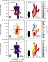 |
Fig. 5 Peak main beam temperatures (top), central velocities (middle), and velocity dispersions (bottom) of the SO2 Gaussian components, separated into σv ≤ 1.8 km s−1 (left) and σv > 1.8 km s−1 (right). The images in the right column focus on a region approximately 250 au in radius from the protostar. Blue and red arrows mark the direction of the outflow. Black ellipses represent the beam size. Crosses (black and white) represent the locations of the SO2 peaks. A scale bar indicates a length of 200 au. |
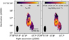 |
Fig. 6 Parameters derived from LTE calculations of all SO2 transitions. Peak positions are marked as in Fig. 1. The black ellipse represents the beam size. A scale bar represents a length of 200 au. Crosses represent the locations of the SO2 peaks. Left: rotational temperature. Right: base 10 logarithm of the SO2 column density. |
Physical properties of the SO2 peaks from nested sampling and LTE analysis.
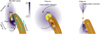 |
Fig. 7 Schematic of the proposed interpretation of SO2 emission: the envelope (purple) impacts the streamer (brown) from the side as the latter falls toward the disk, causing a higher density and temperature and generating a SO2 peak ar around 400 au from the protostar (white star). It is unclear if peak 1, which is a shock, potentially in the disk-envelope interface, is caused by the streamer or not. The peaks are shown with white explosion signs and labeled. The black arrows indicate the direction of envelope infall-rotation motions. The white arrow indicates the general motion of the streamer. Black and cyan contours show the brightness distribution of SO2 and H2CO, respectively, from Fig. 1. |
4 Discussion
4.1 Origin of the SO2 peaks
The two SO2 peaks can have different physical origins. As was stated in Sect. 3.1, peak 1 lies close to the base of the outflow, and the kinematic analysis of the SO2 brightest line shows that emission in this region follows the expected motion from an IRE. Peak 2, however, is not associated with CO emission from the outflow base (Fig. A.1) and its peak velocity is blueshifted with respect to the expected IRE motion. The size of the disk is too small (radius < 30 au, Segura-Cox et al. 2018) to influence the gas velocity at this position.
We propose that peak 2 is caused by the shock between the inner envelope and the streamer as the latter moves toward the protostar, but before reaching the disk region of Per-emb 50. This is mostly supported by the shift of SO and SO2 emission toward blueshifted velocities close to the streamer. H2CO emission tracing the streamer is accelerating toward blueshifted velocities, whereas the infall-rotation of the envelope, traced through both SO ad SO2 toward the south, is redshifted (Fig. 3). The streamer and the SO2 peaks are not co-spatial because we are observing a flattened envelope from a close to edge-on configuration (i ~ 70 deg, Segura-Cox et al. 2018; Zhang et al. 2023), and the streamer hits one side of the inner envelope at an angle. We suggest that, as the streamer moves toward the disk, it pushes the envelope from one side, causing material to compresses within the envelope and heat up. Thus, the relative motion between streamer and envelope causes a shock front, which we observe thanks to the SO and SO2 peak 2. If we were to observe the disk-envelope-system face on, SO2 and H2CO emission would be co-spatial. This picture is visualized in Fig. 7. SO and SO2 have been associated with shocks produced by streamers in other sources (Artur de la Villarmois et al. 2022; Garufi et al. 2022; Flores et al. 2023; Tanious et al. 2024). Other shock-tracing molecules such as SiO (which is included in the PRODIGE setup) are not detected toward Per-emb 50, which suggests that the shock is not strong enough to sputter Si material (e.g., Schilke et al. 1997). This scenario of shocked compression is consistent with the observed polarization vectors toward peak 2 seen by Zhang et al. (2023), who suggest that the different polarization fractions toward peak 2 with respect to the disk are due to a slow shock changing the properties of dust in that region.
SO2 peak 1 could also be due to the streamer, but given the presence of CO (Fig. A.1) and its proximity to the protostar (about 180 au), there are other possibilities that explain their presence. First, this could be a shock at the disk-envelope interface due to the infall from the envelope to the disk (e.g., Terebey et al. 2025). This is supported by the fact that we see SO2 emission consistent with rotation both to the north and south of the protostar (Fig. 5). This phenomenon has been used to explain the emergence of molecular emission close to the disk boundary in other protostars (Sakai et al. 2014). The offset, peak emission of SO and SO2 in this scenario can be explained by asymmetries in the envelope mass distribution; this asymmetry can be caused by the streamer, as is suggested in Zhang et al. (2023), but can also be related to an asymmetric gas distribution in the envelope (e.g., Sakai et al. 2016). Recently, Liu et al. (2025) showed that SO and SO2 associated with streamers and envelope infall can be observed simultaneously. Second, it could be produced by a shock between the outflow and the envelope material at a distance of 100 to 200 au. This is supported by the spatial coincidence between SO2 and SO peak 1 with the outflow emission traced by CO (Figs. A.1 and A.2). SO is known to trace outflows in young embedded sources (Artur de la Villarmois et al. 2023), and SO enhancements have been seen in outflow interactions with envelope material (Oya et al. 2025). A final possibility is that SO and SO2 near the protostar are tracing a disk wind. Both molecules have been used to detect and characterize disk winds in protostars (e.g., Tabone et al. 2017), and the brightness distribution tracing the disk wind can be asymmetric (van’t Hoff et al. 2023; Mori et al. 2025). Observations with higher spatial resolution are needed to determine which scenario can explain the brightest SO2 peak.
4.2 Shock conditions
Assuming that both peaks are generated by shocks, we made a rough estimate of the shock conditions based on the geometry of the system and the column densities of SO2 and SO. We obtained an estimate of the column density of SO (N(SO)) at the location of the SO2 peaks by fitting the observed SO 55–44 beam-averaged spectra at the location of both peaks using XCLASS. We used a similar procedure as in Sect. 3.4, but we fixed the rotational temperatures to the ones found for SO2 (Table 2), as Trot cannot be constrained using only one SO transition. For peak 1, we obtain N(SO) ≈ 4 × 1015 cm−2, and for peak 2, N(SO) ≈ 3 × 1015 cm−2. Comparing with the LTE column densities obtained for SO2, the abundance ratio SO2/SO is around 0.3 for peak 2 and about 0.2 for peak 1. Comparing with the shock models from van Gelder et al. (2021, their Fig. 10), the ratios roughly agree with a low-velocity shock (~2–3 km s−1), or an intermediate-velocity shock (~5–7 km s−1) in the case in which the pre-shock volume density was lower (around 106 cm−3) than the current (post-shock) density (~107 cm−3, Sect. 3.4). Given that our non-LTE values give a lower limit of around 107 cm−3 for the current density (Appendix D), it is possible that the density of the gas increased locally thanks to the shock between envelope and streamer. According to this model, the temperature increase due to the shock could enhance SO and SO2 via their gas phase formation routes.
The derived velocities for the streamer and the envelope are consistent with the shock scenario suggested by the LTE conditions. To estimate the absolute velocity difference, we obtained the velocity vectors for the free-falling trajectory of the streamer, using the parameters from Valdivia-Mena et al. (2022), and the velocity vectors for the IRE model from Zhang et al. (2023). Then, we selected the IRE locations that intersected with the streamer model. The total, three-dimensional velocity difference between the modeled IRE and the modeled streamer at 400 au from the protostar is ≈2.6 km s−1. This velocity difference is consistent within the expected velocity for the shock based on the abundance ratio described above. This is also the case the centrifugal radius of the streamer, at about 250 au: here, the absolute difference in velocity between both models is about 4 km s−1. The higher velocity is consistent with a lower SO2/SO abundance ratio under low-velocity shocks (van Gelder et al. 2021).
These are rough estimates of the potential shock conditions. Both the IRE from Zhang et al. (2023) and the best free-fall model from Valdivia-Mena et al. (2022) are estimations based on visual inspection instead of fitting, so the velocities obtained from them might not be the true velocities of the envelope and the streamer. Also, the comparison with van Gelder et al. (2021) is an estimate, given our LTE approximation of the column densities. Nevertheless, our observations are not consistent with a stronger or faster shock. Given that SiO was not detected toward this source, as was mentioned previously, the velocity of the streamer with respect to the envelope is not enough to sputter Si from the dust grains (Schilke et al. 1997; Caselli et al. 1997; Jiménez-Serra et al. 2008). This low velocity is also not enough to sputter ice; therefore, any desorption in this region may be via thermal desorption due to the increase in temperature after the shock, in particular of more volatile species (Aota et al. 2015). This can affect the abundances of species with lower binding energies, such as CO and CH4, and thus modify the abundance of this molecule in regions impacted by streamers. We note that streamers can produce stronger shocks in other regions, such as in IRS 63, where the abundance of D2CO gas can be explained by the streamer shock as it sputters ices (Podio et al. 2024). Further investigation of the impact locations of streamers toward disks and inner envelopes is needed to understand the range of chemical changes they can produce.
5 Summary
In this work, we present NOEMA observations with the most extended configuration (A) toward the Class I protostar Per-emb 50. We analyzed three rotational transitions of SO2 wth Eup from 19 to 93 K, together with SO 55–44, H2CO 30,3–20,2 and CO 2–1 line emission. We find that SO2 is located offset from the protostar in two peaks toward the southwest: one at about 180 au (peak 1) and another at 400 au (peak 2). This paper focuses on analyzing the physical conditions based on SO2 and SO to explain their appearance. The physical interpretation of the molecular emission is summarized in Fig. 7 and explained below.
SO2 emission traces part of an IRE, traced by a narrow (σv ~ 0.7–0.8 km s−1) Gaussian component, as well as potential disk emission based on its central velocities, traced by a wider SO2 component (σv ≥ 2 km s−1). Both peak 1 and 2 are part of the narrow Gaussian component. We estimated the physical conditions traced by SO2 using only the narrow components to separate potential disk emission from the peaks. An LTE analysis of the three SO2 transitions resulted in high column densities for SO2 (up to 1015 cm−2 for the brightest peak) and temperatures of about 64 K for peak 1 and 46 K for peak 2. A non-LTE analysis corroborated the high column densities and showed that the volume density in peak 2 needs to be at least 107 cm−3 to explain the presence of the three transitions.
Our analysis of SO2 and SO emission and abundance ratios suggest that peak 2, the farthest away from the protostar, is consistent with a slow shock (~3 km s−1) inside the inner envelope. Given the location of the peak (400 au away) and the presence of the streamer head toward the east of this peak, we propose that there is a shock due to the difference between the streamer and the envelope velocities toward the southwest. The disk-envelopestreamer system is edge-on with respect to the observer, thus we observe the shock from one side, where the envelope is compressed and heated due to the impact.
SO2 peak 1 might also be caused by the streamer, but there are also other possibilities, such as shocks in the disk-envelope interface or interactions with the outflow. This peak is consistent with envelope motion (comparing to an IRE model) and is potentially located at the outer part of the disk (~180 au). The abundance ratios are also consistent with slow shocks in this region. Higher-resolution data that resolves the gas disk are needed to investigate this peak’s nature further.
Our results indicate that streamers can affect the structure of both disks and envelopes: a streamer can affect the envelope as it comes into contact with the latter, causing a shocked and compressed layer where the two meet, and it can also impact the disk near its landing. Our observations of Per-emb 50 show shocks due to a streamer and possibly also at the disk-envelope interface simultaneously, similar to observations in other embedded protostars (Liu et al. 2025). Our results suggest that streamers can have a diversity of effects when infalling toward a young protostar, opening new avenues to explore the chemical inheritance from the ISM onto planet-forming disks.
Acknowledgements
We thank the anonymous referee for their constructive comments during peer review. M.T.V.-M. thanks Marta de Simone, Pooneh Nazari and Suchitra Narayanan for their insightful discussions about the contents of this article. M.T.V.-M, J.E.P., C.G., P.C., Y.L., M.J.M., L.A.B., D.S., Y.-R.C., R.F. and K.S. acknowledge the support by the Max Planck Society. This project is co- funded by the European Union (ERC, SUL4LIFE, grant agreement No. 101096293). A.F. also thanks project PID2022-137980NB-I00 funded by the Spanish Ministry of Science and Innovation/State Agency of Research MCIN/AEI/10.13039/501100011033 and by “ERDF A way of making Europe”. D.S. was funded by the Deutsche Forschungsgemeinschaft (DFG, German Research Foundation) – project number: 550639632. I.J.-S. acknowledges funding from grant PID2022-136814NB-I00 funded by the Spanish Ministry of Science, Innovation and Universities/State Agency of Research MICIU/AEI/10.13039/501100011033 and by “ERDF/EU”. The authors thank the IRAM staff at the NOEMA observatory for their support in the observations and data calibration. This work is based on observations carried out under projects number W22AH and L19MB with the IRAM NOEMA Interferometer. IRAM is supported by INSU/CNRS (France), MPG (Germany) and IGN (Spain). IRE models were calculated using FERIA (Oya et al. 2022) available at https://github.com/YokoOya/FERIA. This research has made use of NASA’s Astrophysics Data System Bibliographic Services.
References
- Aota, T., Inoue, T., & Aikawa, Y. 2015, ApJ, 799, 141 [NASA ADS] [CrossRef] [Google Scholar]
- Artur de la Villarmois, E., Guzmán, V. V., Jørgensen, J. K., et al. 2022, A&A, 667, A20 [NASA ADS] [CrossRef] [EDP Sciences] [Google Scholar]
- Artur de la Villarmois, E., Guzmán, V. V., Yang, Y. L., Zhang, Y., & Sakai, N. 2023, A&A, 678, A124 [NASA ADS] [CrossRef] [EDP Sciences] [Google Scholar]
- Aso, Y., Kwon, W., Ohashi, N., et al. 2023, ApJ, 954, 101 [NASA ADS] [CrossRef] [Google Scholar]
- Balança, C., Spielfiedel, A., & Feautrier, N. 2016, MNRAS, 460, 3766 [CrossRef] [Google Scholar]
- Buchner, J., Georgakakis, A., Nandra, K., et al. 2014, A&A, 564, A125 [NASA ADS] [CrossRef] [EDP Sciences] [Google Scholar]
- Caselli, P., Hartquist, T. W., & Havnes, O. 1997, A&A, 322, 296 [NASA ADS] [Google Scholar]
- Ceccarelli, C., Codella, C., Balucani, N., et al. 2023, in Astronomical Society of the Pacific Conference Series, 534, Protostars and Planets VII, eds. S. Inutsuka, Y. Aikawa, T. Muto, K. Tomida, & M. Tamura, 379 [Google Scholar]
- Draine, B. T., Roberge, W. G., & Dalgarno, A. 1983, ApJ, 264, 485 [CrossRef] [Google Scholar]
- Drozdovskaya, M. N., van Dishoeck, E. F., Jørgensen, J. K., et al. 2018, MNRAS, 476, 4949 [Google Scholar]
- Endres, C. P., Schlemmer, S., Schilke, P., Stutzki, J., & Müller, H. S. 2016, J. Mol. Spectrosc., 327, 95, new Visions of Spectroscopic Databases, Volume II [NASA ADS] [CrossRef] [Google Scholar]
- Flores, C., Ohashi, N., Tobin, J. J., et al. 2023, ApJ, 958, 98 [NASA ADS] [CrossRef] [Google Scholar]
- Garufi, A., Podio, L., Codella, C., et al. 2022, A&A, 658, A104 [CrossRef] [EDP Sciences] [Google Scholar]
- Gieser, C., Pineda, J. E., Segura-Cox, D. M., et al. 2024, A&A, 692, A55 [NASA ADS] [CrossRef] [EDP Sciences] [Google Scholar]
- Gieser, C., Caselli, P., Segura-Cox, D. M., et al. 2025, A&A, 701, A165 [NASA ADS] [CrossRef] [EDP Sciences] [Google Scholar]
- Ginsburg, A., & Mirocha, J. 2011, PySpecKit: Python Spectroscopic Toolkit, Astrophysics Source Code Library [record ascl:1109.001] [Google Scholar]
- Ginsburg, A., Sokolov, V., de Val-Borro, M., et al. 2022, AJ, 163, 291 [NASA ADS] [CrossRef] [Google Scholar]
- Hennebelle, P., Lesur, G., & Fromang, S. 2017, A&A, 599, A86 [NASA ADS] [CrossRef] [EDP Sciences] [Google Scholar]
- Högbom, J. A. 1974, A&AS, 15, 417 [Google Scholar]
- Hsieh, T. H., Segura-Cox, D. M., Pineda, J. E., et al. 2023, A&A, 669, A137 [NASA ADS] [CrossRef] [EDP Sciences] [Google Scholar]
- Hsieh, C.-H., Arce, H. G., Maureira, M. J., et al. 2025a, A&A, 700, A235 [NASA ADS] [CrossRef] [EDP Sciences] [Google Scholar]
- Hsieh, T. H., Pineda, J. E., Segura-Cox, D. M., et al. 2025b, A&A, 696, A1 [NASA ADS] [CrossRef] [EDP Sciences] [Google Scholar]
- Jiménez-Serra, I., Caselli, P., Martín-Pintado, J., & Hartquist, T. W. 2008, A&A, 482, 549 [NASA ADS] [CrossRef] [EDP Sciences] [Google Scholar]
- Kido, M., Yen, H.-W., Sai, J., et al. 2025, ApJ, 985, 166 [Google Scholar]
- Kuznetsova, A., Bae, J., Hartmann, L., & Mac Low, M.-M. 2022, ApJ, 928, 92 [NASA ADS] [CrossRef] [Google Scholar]
- Liu, X. C., van Dishoeck, E. F., Hogerheijde, M. R., et al. 2025, A&A, 701, A141 [NASA ADS] [CrossRef] [EDP Sciences] [Google Scholar]
- Manara, C. F., Morbidelli, A., & Guillot, T. 2018, A&A, 618, L3 [NASA ADS] [CrossRef] [EDP Sciences] [Google Scholar]
- Maureira, M. J., Gong, M., Pineda, J. E., et al. 2022, ApJ, 941, L23 [NASA ADS] [CrossRef] [Google Scholar]
- Möller, T., Endres, C., & Schilke, P. 2017, A&A, 598, A7 [NASA ADS] [CrossRef] [EDP Sciences] [Google Scholar]
- Mori, S., Bai, X.-N., & Tomida, K. 2025, ApJ, 992, 85 [Google Scholar]
- Neufeld, D. A., & Hollenbach, D. J. 1994, ApJ, 428, 170 [Google Scholar]
- Oya, Y., López-Sepulcre, A., Sakai, N., et al. 2019, ApJ, 881, 112 [Google Scholar]
- Oya, Y., Kibukawa, H., Miyake, S., & Yamamoto, S. 2022, PASP, 134, 094301 [Google Scholar]
- Oya, Y., Saiga, E., Miotello, A., et al. 2025, ApJ, 980, 263 [Google Scholar]
- Pineda, J. E., Segura-Cox, D., Caselli, P., et al. 2020, Nat. Astron., 4, 1158 [NASA ADS] [CrossRef] [Google Scholar]
- Pineda, J. E., Arzoumanian, D., Andre, P., et al. 2023, in Astronomical Society of the Pacific Conference Series, 534, Protostars and Planets VII, eds. S. Inutsuka, Y. Aikawa, T. Muto, K. Tomida, & M. Tamura, 233 [Google Scholar]
- Podio, L., Ceccarelli, C., Codella, C., et al. 2024, A&A, 688, L22 [NASA ADS] [CrossRef] [EDP Sciences] [Google Scholar]
- Pontoppidan, K. M., Salyk, C., Bergin, E. A., et al. 2014, in Protostars and Planets VI, eds. H. Beuther, R. S. Klessen, C. P. Dullemond, & T. Henning, 363 [Google Scholar]
- Sakai, N., Sakai, T., Hirota, T., et al. 2014, Nature, 507, 78 [Google Scholar]
- Sakai, N., Oya, Y., López-Sepulcre, A., et al. 2016, ApJ, 820, L34 [NASA ADS] [CrossRef] [Google Scholar]
- Schilke, P., Walmsley, C. M., Pineau des Forets, G., & Flower, D. R. 1997, A&A, 321, 293 [NASA ADS] [Google Scholar]
- Segura-Cox, D. M., Looney, L. W., Tobin, J. J., et al. 2018, ApJ, 866, 161 [Google Scholar]
- Segura-Cox, D. M., Schmiedeke, A., Pineda, J. E., et al. 2020, Nature, 586, 228 [NASA ADS] [CrossRef] [Google Scholar]
- Sheehan, P. D., Tobin, J. J., Federman, S., Megeath, S. T., & Looney, L. W. 2020, ApJ, 902, 141 [Google Scholar]
- Sokolov, V., Pineda, J. E., Buchner, J., & Caselli, P. 2020, ApJ, 892, L32 [NASA ADS] [CrossRef] [Google Scholar]
- Speedie, J., Dong, R., Teague, R., et al. 2025, ApJ, 981, L30 [Google Scholar]
- Tabone, B., Cabrit, S., Bianchi, E., et al. 2017, A&A, 607, L6 [NASA ADS] [CrossRef] [EDP Sciences] [Google Scholar]
- Taniguchi, K., Pineda, J. E., Caselli, P., et al. 2024, ApJ, 965, 162 [Google Scholar]
- Tanious, M., Le Gal, R., Neri, R., et al. 2024, A&A, 687, A92 [NASA ADS] [CrossRef] [EDP Sciences] [Google Scholar]
- Terebey, S., Sandoval Ascencio, L., Flores-Rivera, L., Turner, N. J., & Barajas, A. 2025, ApJ, 990, 53 [Google Scholar]
- Tobin, J. J., & Sheehan, P. D. 2024, ARA&A, 62, 203 [Google Scholar]
- Tobin, J. J., Hartmann, L., Bergin, E., et al. 2012, ApJ, 748, 16 [Google Scholar]
- Tychoniec, Ł., Manara, C. F., Rosotti, G. P., et al. 2020, A&A, 640, A19 [NASA ADS] [CrossRef] [EDP Sciences] [Google Scholar]
- Valdivia-Mena, M. T., Pineda, J. E., Segura-Cox, D. M., et al. 2022, A&A, 667, A12 [NASA ADS] [CrossRef] [EDP Sciences] [Google Scholar]
- Valdivia-Mena, M. T., Pineda, J. E., Segura-Cox, D. M., et al. 2023, A&A, 677, A92 [NASA ADS] [CrossRef] [EDP Sciences] [Google Scholar]
- van der Tak, F. F. S., Black, J. H., Schöier, F. L., Jansen, D. J., & van Dishoeck, E. F. 2007, A&A, 468, 627 [NASA ADS] [CrossRef] [EDP Sciences] [Google Scholar]
- van Gelder, M. L., Tabone, B., van Dishoeck, E. F., & Godard, B. 2021, A&A, 653, A159 [CrossRef] [EDP Sciences] [Google Scholar]
- van’t Hoff, M. L. R., Tobin, J. J., Li, Z.-Y., et al. 2023, ApJ, 951, 10 [CrossRef] [Google Scholar]
- Vastel, C., Alves, F., Ceccarelli, C., et al. 2022, A&A, 664, A171 [NASA ADS] [CrossRef] [EDP Sciences] [Google Scholar]
- Zamponi, J., Maureira, M. J., Zhao, B., et al. 2021, MNRAS, 508, 2583 [NASA ADS] [CrossRef] [Google Scholar]
- Zhang, Z. E., Yang, Y.-l., Zhang, Y., et al. 2023, ApJ, 946, 113 [NASA ADS] [CrossRef] [Google Scholar]
- Zucker, C., Schlafly, E. F., Speagle, J. S., et al. 2018, ApJ, 869, 83 [NASA ADS] [CrossRef] [Google Scholar]
Appendix A SO2 emission in comparison to other molecules
Figure A.1 shows the integrated intensity of the SO2 transitions 42,2 − 31,3 and 123,9 − 122,10. Emission from these transitions is weaker than the 111,11–100,10 transition, but the distribution of the peaks is the same. We also plot CO contours and H2CO contours over the SO2 transitions to compare their morphology. Redshifted CO emission coincides spatially with SO2 peak 1, although its maximum is closer to the protostar. H2CO emission is not coincident with SO2 emission, with its maximum emission toward the southwest of the protostar.
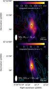 |
Fig. A.1 Integrated intensity of SO2 42,2 − 31,3 and 123,9 − 122,10, compared with CO and H2CO emission near the protostar. All SO2 transitions are integrated in the same velocity range as in Fig. 1. Crosses mark the locations of peaks 1 and 2. Top: SO2 42,2 − 31,3 integrated intensity map. Red and blue contours mark the same CO contours as in Fig. 1. Bottom: SO2 123,9 − 122,10 integrated intensity map. Blue contours represent the H2CO integrated intensity, with contours drawn at 3,5 and 10 times the rms of the map (0.7 K km s−1). The dashed line represents the direction of the PV diagram in Fig. 2. |
We compared the emission from SO and SO2 with the expected emission from an IRE (IRE). We first created a simulated data cube using FERIA (Oya et al. 2022), with the IRE parameters found by Zhang et al. (2023) as input: a density power law α = −1.5, envelope height scale h(r)/r = 0.2, an outer radius of 2.4″, a centrifugal barrier distance of 0.4″ (119 au), projected centrifugal velocity vrot,max cos(i) = 3.5 km s−1 and a disk inclination angle of 10 deg (Table 4 of Zhang et al. 2023). We then obtained a PV diagram of this simulated IRE using the same path as for SO and SO2. The resulting PV diagrams of the simulated IRE are plotted in white contours in Fig. 2. We did not include the Keplerian rotating disk in the IRE model because we focused only on the bright, resolved SO2 emission. We note that the parameters from Zhang et al. (2023) return a central mass of 0.85 M⊙, which differs from the mass of 1.7 M⊙ determined in Valdivia-Mena et al. (2022). The centrifugal barrier radius rcb and the rotation velocity at that location vrot,max are related by the central mass by
![Mathematical equation: $\[r_{\mathrm{cb}}=\frac{2 G M_*}{v_{\mathrm{rot}, \max }^2},\]$](/articles/aa/full_html/2026/05/aa57958-25/aa57958-25-eq6.png) (A.1)
(A.1)
based on the equations of the IRE model in Oya et al. (2022). After deprojecting the velocity at the centrifugal barrier by cos(i), the resulting mass from the IRE model parameters is 0.85 M⊙. The difference occurs because both masses are estimates based on adjusting models to the observations by visual inspection, and the observations in both cases do not resolve the disk. Therefore, the mass of Per-emb 50 is not well constrained.
Figure A.2 shows the spectra of SO, SO2 and CO at the SO2 peak locations. CO has no emission observed between approximately 7 and 9.5 km s−1 due to large-scale cloud emission not recovered by our NOEMA observations. SO and SO2 emission in peak 1 have a velocity of 9.8 km s−1, close to the apparent peak of CO at that location (at 10.4 km s−1), and so it is possible that SO and SO2 emission are associated with the outflow at that location. However, CO emission in peak 2 is dominated by large-scale emission and is farther away from the apparent redshifted outflow lobe base (Fig. A.1 top).
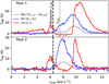 |
Fig. A.2 Same as Fig. 3 but with CO 2 − 1 spectra at the location of the SO2 peaks. CO emission is drawn in solid red lines. The vertical dashed-dotted line marks the systemic velocity of the protostar (7.5 km s−1), whereas the thick dashed line marks the velocity of the streamer at the same distance from the protostar (in radius) as peak 2 (6.45 km s−1, Fig. B.1 middle. |
Appendix B Streamer kinematics
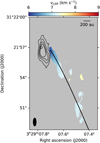 |
Fig. B.1 Best-fit central velocity for the Gaussian fit to H2CO 30,3–20,2, for emission with S/N> 5. Black contours mark 5, 10, 15 and 20 times the rms level (0.8 K km s−1) of the SO2 111,11–100,10 integrated intensity image from Fig. 1. The black curve represents the streamer trajectory from Valdivia-Mena et al. (2022). An ellipse in the bottom-left corner represents the beam. The scale bar in the top right shows a length of 200 au. |
The H2CO spectra across the whole length of the streamer show one clear Gaussian peak, consistent with previous results from Valdivia-Mena et al. (2022). We fit one Gaussian to each spectrum with S/N> 5 using pyspeckit (Ginsburg & Mirocha 2011; Ginsburg et al. 2022). The best-fit central velocities v for the new NOEMA map are shown in Fig. B.1. The velocities decrease down to approximately 6.2 km s−1 at the tip of the streamer. However, at the projected distance of SO2 peak 2 (400 au), the average velocity in a beam of H2CO emission is 6.45 km s−1. We note that there is no H2CO emission at the location of SO2 peaks.
Appendix C Nested sampling fits of SO2
We fit up to three Gaussian curves to each of the spectra in the brightest SO2 transition (111,11–100,10) which has S/N > 5. We applied Bayesian model selection through the nested sampling algorithm to fit and select the number of components that at the same time. A full description of this line decomposition method is found in Sokolov et al. (2020). We used the pymultinest Python package (Buchner et al. 2014) to run the nested sampling algorithm in Python. We used pyspecnest (Sokolov et al. 2020) to introduce pyspeckit models to the pymultinest code. We selected the best model by using the standard threshold of ![Mathematical equation: $\[\ln(K_{n-1}^{n})=5\]$](/articles/aa/full_html/2026/05/aa57958-25/aa57958-25-eq7.png) , where n is the number of Gaussian components of the model being compared against a model with n − 1 components. In this case, n = 0 corresponds to background noise. Figure C.1 shows the number of Gaussian components that best fit each pixel of the SO2 111,11–100,10 data cube. Close to the protostar, there are two Gaussian components recognized through nested sampling, and a few pixels toward the west of the continuum peak are best fit with three Gaussians.
, where n is the number of Gaussian components of the model being compared against a model with n − 1 components. In this case, n = 0 corresponds to background noise. Figure C.1 shows the number of Gaussian components that best fit each pixel of the SO2 111,11–100,10 data cube. Close to the protostar, there are two Gaussian components recognized through nested sampling, and a few pixels toward the west of the continuum peak are best fit with three Gaussians.
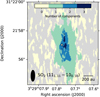 |
Fig. C.1 Number of Gaussian components that best fit the SO2 111,11–100,10 spectra. The white star marks the position of the protostar. The black ellipse in the bottom-left corner shows the size of the beam. A scale bar represents a physical size of 200 au. |
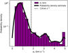 |
Fig. C.2 Histogram and probability density estimate of the σv values obtained for all Gaussian fits to the SO2 line cube. The histogram is normalized by density. The dashed line marks the position of the first inflection point of the PDE (1.8 km s−1). |
Figure C.2 shows the distribution of σv values from all Gaussian components in the map, together with the estimated PDF of σv. We first made a histogram of the obtained σv values for all Gaussian fits found in the SO2 map. Then, we estimated the PDF of the σv distribution by calculating its Kernel Density Estimate (KDE), using the scipy.stats function gaussian_kde. The majority Gaussian components have σv < 1, with a peak around 0.7 km s−1, but there are also additional peaks of σv, one at around 2.2 km s−1 and a third around 3.1 km s−1. We located the inflection point between the first two peaks at σv = 1.8 km s−1.
Appendix D Non-LTE calculations
We calculated line ratios between the different transitions of SO2 in grids of kinetic temperature and SO2 column density, using the non-LTE radiative transfer code RADEX (van der Tak et al. 2007). For nH2 = 106 cm−3, RADEX was run with a set of 50 equally spaced temperatures from 30 to 100 K and 50 equally spaced column density values from 5 × 10¹² to 5 × 1015 cm−2. For nH2 = 107 and 108 cm−3, the grid was run with 50 equally spaced temperatures from 20 to 80 K and 50 equally spaced column density values from 1014 to 5 × 1016 cm−2. Combinations with column density higher than 5 × 1015 cm−2 for nH2 = 106 cm−3 did not converge. Besides these values, we used the default values for the radiation model (Uniform sphere) and background temperature (2.73 K).
We recovered the line intensities from the RADEX outputs for each combination of parameters. It was not possible to replicate the line intensities for the three transitions assuming a beam filling fraction of 1. To avoid assuming a beam filling factor for emission of an unknown size, we instead used the line ratios of the different transitions to comper with our observed SO2 emission. We plotted where the line ratios obtained from our SO2 observations of peak 2 lie in the RADEX grids. The resulting positions in the Tkin − N(SO2) grids for each nH2 are shown in Fig. D.1.
Our RADEX calculations show that there is no Tkin − N(SO2) possible combination for nH2 = 106 cm−3 where the line ratios can coexist. For nH2 = 107 and 108 cm−3, there exist an inter-section area. The line ratios intersect at Tkin = 51 K and log N(SO2) = 15.4 cm−2 for nH2 = 107 cm−3, and at Tkin = 45 K and log N(SO2) = 15.0 cm−2 for nH2 = 108 cm−3, so the higher nH2, the lower the required Tkin − N(SO2) to replicate the observed line ratios.
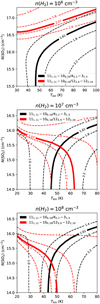 |
Fig. D.1 Line ratios between SO2 111,11 − 100,10, 42,2 − 31,3 and 123,9 − 122,10 transitions resulting from different combinations of Tkin − N(SO2) obtained with RADEX. Black lines show the resulting 111,11–100,10 over 42,2–31,3 line ratio, whereas red lines show the 111,11–100,10 over 123,9–122,10 line ratio. The thick black and red lines mark the line ratios found in the spectra of peak 2. The dashed black and red lines indicate where other line ratio values are located in the grid. Top: results for nH2 = 106 cm−3. Middle: results for nH2 = 107 cm−3. Bottom: results for nH2 = 108 cm−3. |
All Tables
All Figures
|
Fig. 1 NOEMA observations of molecular emission toward Per-emb 50. Left: integrated intensity of SO2 111,11–100,10 between 6.5 and 12 km s−1. Black crosses show the locations of the SO2 peaks, labeled as peak 1 and peak 2. Cyan contours represent the H2CO 30,3–20,2 integrated intensity between 5 and 8 km s−1, drawn in steps of 3, 5, and 10 times the rms of the integrated image (0.7 K km s−1). Right: integrated intensity of SO 55–44 between 0 and 13 km s−1. The red and cyan contours are the CO integrated intensity in redshifted and blueshifted channels, respectively, with respect to the protostar’s vLSR (7.5 km s−1). Blueshifted channels are integrated between −4.3 and 5.3 km s−1, and redshifted channels between 10 and 20 km s−1. Contours are drawn at 5–45 times the rms of the integrated images (4.7 K km s−1) in steps of 10. Red and blue arrows indicate the direction of the outflow. The dashed line represents the direction of the PV diagram in Fig. 2. The white star marks the position of the continuum peak. The filled white ellipse represents the beam size. A scale bar in the bottom right corner represents a physical scale of 200 au. |
| In the text | |
|
Fig. 2 Position velocity diagrams of SO2 and SO using the path shown in Fig. 1. SO2 transitions are in order of increasing upper energy levels, Eup. From left to right: SO2 42,2–31,3, SO2 111,11–100,10, SO2 123,9–122,10, SO 55–44. White contours show the normalized intensity PV diagrams for an IRE, obtained with FERIA (Oya et al. 2022). |
| In the text | |
|
Fig. 3 Spectra of SO 55–44 (blue) and SO2 111,11–100,10 (gray) at the two resolved peak positions, together with the spectra obtained from FERIA, normalized to the SO intensity at the peak velocity of the IRE. The vertical dash-dotted line marks the systemic velocity of the protostar (7.5 km s−1), whereas the thick dashed line marks the velocity of the streamer at the same distance from the protostar (in radius) as peak 2 (6.45 km s−1; Appendix B). |
| In the text | |
|
Fig. 4 SO2 spectra (gray) at the location of the peaks together with the best-fit (dashed black lines) Gaussian models. Peak 1 has two Gaussian components, a narrow one (orange, σv < 1.8 km s−1) and a wide one (blue, σv > 1.8 km s−1), whereas peak 2 has just one component (narrow). |
| In the text | |
|
Fig. 5 Peak main beam temperatures (top), central velocities (middle), and velocity dispersions (bottom) of the SO2 Gaussian components, separated into σv ≤ 1.8 km s−1 (left) and σv > 1.8 km s−1 (right). The images in the right column focus on a region approximately 250 au in radius from the protostar. Blue and red arrows mark the direction of the outflow. Black ellipses represent the beam size. Crosses (black and white) represent the locations of the SO2 peaks. A scale bar indicates a length of 200 au. |
| In the text | |
|
Fig. 6 Parameters derived from LTE calculations of all SO2 transitions. Peak positions are marked as in Fig. 1. The black ellipse represents the beam size. A scale bar represents a length of 200 au. Crosses represent the locations of the SO2 peaks. Left: rotational temperature. Right: base 10 logarithm of the SO2 column density. |
| In the text | |
|
Fig. 7 Schematic of the proposed interpretation of SO2 emission: the envelope (purple) impacts the streamer (brown) from the side as the latter falls toward the disk, causing a higher density and temperature and generating a SO2 peak ar around 400 au from the protostar (white star). It is unclear if peak 1, which is a shock, potentially in the disk-envelope interface, is caused by the streamer or not. The peaks are shown with white explosion signs and labeled. The black arrows indicate the direction of envelope infall-rotation motions. The white arrow indicates the general motion of the streamer. Black and cyan contours show the brightness distribution of SO2 and H2CO, respectively, from Fig. 1. |
| In the text | |
|
Fig. A.1 Integrated intensity of SO2 42,2 − 31,3 and 123,9 − 122,10, compared with CO and H2CO emission near the protostar. All SO2 transitions are integrated in the same velocity range as in Fig. 1. Crosses mark the locations of peaks 1 and 2. Top: SO2 42,2 − 31,3 integrated intensity map. Red and blue contours mark the same CO contours as in Fig. 1. Bottom: SO2 123,9 − 122,10 integrated intensity map. Blue contours represent the H2CO integrated intensity, with contours drawn at 3,5 and 10 times the rms of the map (0.7 K km s−1). The dashed line represents the direction of the PV diagram in Fig. 2. |
| In the text | |
|
Fig. A.2 Same as Fig. 3 but with CO 2 − 1 spectra at the location of the SO2 peaks. CO emission is drawn in solid red lines. The vertical dashed-dotted line marks the systemic velocity of the protostar (7.5 km s−1), whereas the thick dashed line marks the velocity of the streamer at the same distance from the protostar (in radius) as peak 2 (6.45 km s−1, Fig. B.1 middle. |
| In the text | |
|
Fig. B.1 Best-fit central velocity for the Gaussian fit to H2CO 30,3–20,2, for emission with S/N> 5. Black contours mark 5, 10, 15 and 20 times the rms level (0.8 K km s−1) of the SO2 111,11–100,10 integrated intensity image from Fig. 1. The black curve represents the streamer trajectory from Valdivia-Mena et al. (2022). An ellipse in the bottom-left corner represents the beam. The scale bar in the top right shows a length of 200 au. |
| In the text | |
|
Fig. C.1 Number of Gaussian components that best fit the SO2 111,11–100,10 spectra. The white star marks the position of the protostar. The black ellipse in the bottom-left corner shows the size of the beam. A scale bar represents a physical size of 200 au. |
| In the text | |
|
Fig. C.2 Histogram and probability density estimate of the σv values obtained for all Gaussian fits to the SO2 line cube. The histogram is normalized by density. The dashed line marks the position of the first inflection point of the PDE (1.8 km s−1). |
| In the text | |
|
Fig. D.1 Line ratios between SO2 111,11 − 100,10, 42,2 − 31,3 and 123,9 − 122,10 transitions resulting from different combinations of Tkin − N(SO2) obtained with RADEX. Black lines show the resulting 111,11–100,10 over 42,2–31,3 line ratio, whereas red lines show the 111,11–100,10 over 123,9–122,10 line ratio. The thick black and red lines mark the line ratios found in the spectra of peak 2. The dashed black and red lines indicate where other line ratio values are located in the grid. Top: results for nH2 = 106 cm−3. Middle: results for nH2 = 107 cm−3. Bottom: results for nH2 = 108 cm−3. |
| In the text | |
Current usage metrics show cumulative count of Article Views (full-text article views including HTML views, PDF and ePub downloads, according to the available data) and Abstracts Views on Vision4Press platform.
Data correspond to usage on the plateform after 2015. The current usage metrics is available 48-96 hours after online publication and is updated daily on week days.
Initial download of the metrics may take a while.