| Issue |
A&A
Volume 709, May 2026
|
|
|---|---|---|
| Article Number | A165 | |
| Number of page(s) | 23 | |
| Section | Planets, planetary systems, and small bodies | |
| DOI | https://doi.org/10.1051/0004-6361/202558011 | |
| Published online | 13 May 2026 | |
Super-Earth masses and stellar abundances from NIRPS reveal tentative evidence for water-rich formation around M dwarfs
1
Department of Physics & Astronomy, McMaster University,
1280 Main St W,
Hamilton,
ON
L8S 4L8,
Canada
2
Institute for Particle Physics and Astrophysics, ETH Zürich,
Otto-Stern-Weg 5,
8093
Zürich,
Switzerland
3
Institut Trottier de recherche sur les exoplanètes, Département de Physique, Université de Montréal, Montréal,
Québec,
Canada
4
Department of Physics, University of Toronto,
Toronto,
ON
M5S 3H4,
Canada
5
Univ. Grenoble Alpes, CNRS, IPAG,
38000
Grenoble,
France
6
Observatoire de Genève, Département d’Astronomie, Université de Genève,
Chemin Pegasi 51,
1290
Versoix,
Switzerland
7
European Southern Observatory (ESO),
Av. Alonso de Cordova 3107, Casilla
19001,
Santiago de Chile,
Chile
8
Observatoire du Mont-Mégantic,
Québec,
Canada
9
Instituto de Astrofísica e Ciências do Espaço, Universidade do Porto, CAUP, Rua das Estrelas,
4150-762
Porto,
Portugal
10
Departamento de Física e Astronomia, Faculdade de Ciências, Universidade do Porto, Rua do Campo Alegre,
4169-007
Porto,
Portugal
11
Department of Earth, Planetary, and Space Sciences, University of California,
Los Angeles,
CA
90095,
USA
12
Department of Physics, McGill University,
3600 rue University,
Montréal,
QC
H3A 2T8,
Canada
13
Department of Earth & Planetary Sciences, McGill University,
3450 rue University,
Montréal,
QC
H3A 0E8,
Canada
14
Centre Vie dans l’Univers, Faculté des sciences de l’Université de Genève,
Quai Ernest-Ansermet 30,
1205
Geneva,
Switzerland
15
Instituto de Astrofísica de Canarias (IAC), Calle Vía Láctea s/n,
38205
La Laguna, Tenerife,
Spain
16
Departamento de Astrofísica, Universidad de La Laguna (ULL),
38206
La Laguna, Tenerife,
Spain
17
Departamento de Física Teórica e Experimental, Universidade Federal do Rio Grande do Norte, Campus Universitário,
Natal,
RN
59072-970,
Brazil
18
European Southern Observatory (ESO),
Karl-Schwarzschild-Str. 2,
85748
Garching bei München,
Germany
19
Space Research and Planetary Sciences, Physics Institute, University of Bern,
Gesellschaftsstrasse 6,
3012
Bern,
Switzerland
20
Consejo Superior de Investigaciones Científicas (CSIC),
28006
Madrid,
Spain
21
Bishop’s Univeristy, Dept of Physics and Astronomy,
Johnson-104E, 2600 College Street,
Sherbrooke,
QC
J1M 1Z7,
Canada
22
Department of Physics, Engineering Physics, and Astronomy, Queen’s University,
99 University Avenue,
Kingston,
ON
K7L 3N6,
Canada
23
Department of Physics and Space Science, Royal Military College of Canada,
13 General Crerar Cres.,
Kingston,
ON
K7P 2M3,
Canada
24
Centro de Astrobiología (CAB), CSIC-INTA, Camino Bajo del Castillo s/n,
28692,
Villanueva de la Cañada (Madrid),
Spain
25
Planétarium de Montréal, Espace pour la Vie,
4801 av. Pierre-de Coubertin, Montréal,
Québec,
Canada
26
Division of Astrophysics, Department of Physics, Lund University,
Box 118,
SE-22 100
Lund,
Sweden
27
Light Bridges S.L., Observatorio del Teide, Carretera del Observatorio, s/n Guimar,
38500,
Tenerife, Canarias,
Spain
28
University Observatory, Faculty of Physics, Ludwig-Maximilians-Universität München,
Scheinerstr. 1,
81679
Munich,
Germany
29
Department of Physics, The University of Warwick,
Gibbet Hill Road,
Coventry
CV4 7AL,
UK
30
Department of Astronomy & Astrophysics, University of Chicago,
5640 South Ellis Avenue,
Chicago,
IL
60637,
USA
31
Laboratoire Lagrange, Observatoire de la Côte d’Azur, CNRS, Université Côte d’Azur,
Nice,
France
★ Corresponding author: This email address is being protected from spambots. You need JavaScript enabled to view it.
Received:
7
November
2025
Accepted:
30
March
2026
Abstract
Tracing the compositional link between terrestrial super-Earths and their host stars provides clues about their dominant formation pathway. By constraining the stellar abundances of refractory elements, we can predict the core mass fractions (CMFs) of their super-Earths. The level of agreement between this prediction and the planetary CMF derived from their masses and radii can reveal past formation processes, such as mantle stripping and water-rich formation plus sequestration in the planet core. We present the first results from the Near Infrared Planet Searcher (NIRPS) GTO CMF subprogram: an intensive radial velocity campaign to refine masses and compute host stellar abundances of three hot super-Earths around M dwarfs (GJ1132 b, GJ1252 b, and LTT 3780 b). We calculated masses of 1.69 ± 0.15 M⊕, 1.54 ± 0.18 M⊕, and 2.34 ± 0.10 M⊕ respectively. We measured the CMFs of these and six further hot super-Earths with masses already available in the literature to a precision of 10–15%. We compared them to CMF predictions made from measuring the Fe, Mg, and Si abundances of their host stars measured from the NIRPS spectra. The CMFs of these planets are smaller than expected from their host stellar abundances to a statistically significant degree. This discrepancy is suggestive of significant reservoirs of water, and while these planets are too hot to harbor surface water, they likely have interior water mass fractions of ~1%.
Key words: techniques: radial velocities / planets and satellites: composition / planets and satellites: detection / planets and satellites: formation / planets and satellites: terrestrial planets / stars: abundances
© The Authors 2026
 Open Access article, published by EDP Sciences, under the terms of the Creative Commons Attribution License (https://creativecommons.org/licenses/by/4.0), which permits unrestricted use, distribution, and reproduction in any medium, provided the original work is properly cited.
This article is published in open access under the Subscribe to Open model. This email address is being protected from spambots. You need JavaScript enabled to view it. to support open access publication.
1 Introduction
It is crucial to characterize the composition of exoplanets for understanding the pathways that drive their formation. Planet formation models predict qualitatively different distributions of small planet compositions between M dwarfs and Sun-like stars, finding that low-mass water-rich planets are expected to be common around M dwarfs, but probably appear with a lower frequency around FGK stars (Miguel et al. 2020; Burn et al. 2021; Venturini et al. 2024). Some observational evidence also supports different planet formation mechanisms around M dwarfs compared to Sun-like stars. For example, the slope of the radius valley around early M dwarfs is markedly shallower (Cloutier & Menou 2020; Gaidos et al. 2024; Bonfanti et al. 2024; Ho et al. 2024; Wanderley et al. 2025), which points toward the emergence of the M dwarf radius valley as a consequence of planet formation processes and not to thermally driven mass loss. In this paradigm, sub-Neptunes are predominantly water-rich worlds and have no H2/He-dominated atmospheres. Additional supporting empirical evidence for a population of water worlds around M dwarfs comes from the detailed characterization of individual planetary systems with masses or atmospheres suggestive of a water-rich composition (e.g., Diamond-Lowe et al. 2022; Piaulet et al. 2023; Cadieux et al. 2024b; Coulombe et al. 2025) and from planet population-level studies based on mass and radius characterization (e.g., Luque & Pallé 2022; Cherubim et al. 2023; Ho et al. 2024; Parc et al. 2024). It remains an open problem, however, to empirically assess the bulk water content of small planets around M dwarfs, and this needs to be addressed for a proper comparison to the predictions of formation models.
Small close-in planets, with their high equilibrium temperatures (Teq ≳ 800 K), are not expected to have a significant condensed surface water layer or a thick atmosphere because surface water would be vaporized and any atmospheric gas would undergo rapid thermal escape (Lopez 2017; Owen & Wu 2017). It is therefore commonly assumed that the interiors of such planets are composed of two components: an iron-dominated core beneath a primarily silicate mantle. The assumption that planets are composed of only two compositional layers avoids the model degeneracy that is introduced when attempting to infer more than two compositional mass fractions from the measured planetary mass and radius alone. The compositions of these terrestrial planets are well described by a single parameter detailing the relative masses of the rocky mantle and iron core: the core mass fraction (CMF). The CMF is defined as the fraction of the total planetary mass contained within its (assumed) differentiated iron core. However, very precisely constrained masses and radii are required to precisely measure planetary CMF values. Even typical measurement precisions of 20% on planet mass and 5% on planet radius result in large CMF uncertainties that approach 20% (Otegi et al. 2020; Plotnykov & Valencia 2024). Ultra-precise masses and radii (to ~10% and ~3% precision, respectively) are needed to recover CMF uncertainties that are useful for studying the compositional connection between planets and their host stars and for constraining planetary formation and evolutionary processes.
The uncertainties in planetary masses or radii mean that we may frequently rely on the refractory abundances of a planetary host star to set a prior on its CMF. Planets form from the same primordial cloud of material as their host stars, such that it is often assumed that the relative chemical abundances of nonvolatiles such as iron, magnesium, and silicon are common between the planet and star. Many studies have used stellar refractory abundances as proxies on planetary compositions (e.g., Dorn et al. 2015; Dorn et al. 2017a,b; Unterborn et al. 2018). As the data quality improved, it became possible to test the strength of this correlation directly (Santos et al. 2015, 2017; Plotnykov & Valencia 2020; Adibekyan et al. 2021; Schulze et al. 2021; Unterborn et al. 2023; Brinkman et al. 2024, 2025; Behmard et al. 2025). However, these studies have focused largely on planets around FGK stars and not on planets around M dwarfs. In addition, these studies have often struggled to draw conclusions for individual planetary systems because of their involved uncertainties, particularly in planetary mass. As a result, they often instead studied planets on a demographics level, which has yielded a variety of results that differ substantially in the strength of the star-planet compositional connection: some studies have found very little evidence for a star-planet compositional connection (e.g., Brinkman et al. 2024), while others have found a very strong correlation between planetary and host stellar composition (e.g., Adibekyan et al. 2021).
Small planets around M dwarfs provide our best chances of measuring the mass and radius of a planet to the precision necessary for composition analysis. Hot super-Earths have small radii and low masses that make them generally difficult to study. Fortunately, small low-mass M dwarfs produce stronger planetary signals in transit and radial velocity (RV) observations, allowing for the precise characterization of the masses and radii of these planets. Conversely, accurate stellar abundances of M dwarfs are difficult to measure. Atomic lines are often hidden or blended with deep molecular bands, which suppress the continuum in many wavelength regimes, particularly in the optical and the near-infrared (NIR) where M dwarfs are brightest (e.g., Souto et al. 2017; Sarmento et al. 2021; Jahandar et al. 2024). This complicates the recovery of accurate stellar abundances for M dwarfs. Previous studies comparing planetary and stellar compositions therefore largely focused on hotter stars. Fortunately, recent advancements in NIR spectrographs (e.g., the Infrared Doppler Instrument (IRD; Tamura et al. 2012), the Habitable-zone Planet Finder Spectrograph (HPF; Mahadevan et al. 2014), the M-dwarf Advanced Radial velocity Observer Of Neighboring eXoplanets (MAROON-X Seifahrt et al. 2018), the SpectroPolarimètre InfraRouge (SPIRou; Donati et al. 2020), and the Near Infrared Planet Searcher (NIRPS; Bouchy et al. 2025)) have allowed us to improve extremely precise mass determinations of these exoplanets while enabling stellar abundance analyses from high-resolution spectroscopy (e.g., Hejazi et al. 2023; Jahandar et al. 2025) that opens new perspectives for the derivation of precise characterization of M dwarf stellar abundances. This, in turn, allows us to directly compare planetary and stellar compositions.
We present the first results of the Near Infrared Planet Searcher (NIRPS; Bouchy et al. 2025) GTO CMF subprogram to measure precise planetary masses and stellar abundances of nine hot super-Earths orbiting M dwarfs. We measured the planetary CMFs and compared those values to the CMFs predicted from the host star refractory abundances to search for evidence of past formation or evolutionary processes. We present intensive RV follow-up observations with NIRPS and HARPS of three planets to improve the precision of their mass measurements, and we additionally measured stellar refractory abundances for them and five other hot super-Earth hosts. Our paper is structured as follows: in Section 2 we discuss our target selection and the data used for our RV and abundance analyses. In Section 3, we discuss how we determined stellar parameters and abundances and report measured abundances for Mg, Si, and Fe (and Ti in some cases). In Section 4 we discuss the RV model we used to determine planetary masses, and in Section 5 we derive the CMFs of our planets from the planetary masses and radii and from stellar abundances. Last, in Section 6 we compare our results and discuss their implications for the compositions of rocky planets around M dwarfs. We conclude with a summary of our findings in Section 7.
2 Observations
All targets in this sample were observed with NIRPS (Bouchy et al. 2025). NIRPS is a NIR echelle spectrograph designed for precision radial velocities, mounted alongside the High Accuracy Radial Velocity Searcher (HARPS; Mayor et al. 2003) optical spectrograph on the ESO 3.6 m telescope at the La Silla Observatory in Chile. NIRPS observes in the YJH bands (980–1800 nm), can be used simultaneously with HARPS, and has two observing modes: a high-accuracy mode (HA; R ≈ 88 000, 0.4″ fiber) and a high-efficiency mode (HE; R ≈ 75 000, 0.9″ fiber). All HARPS observations taken simultaneously with NIRPS used for the RV analysis in this paper were taken in HE mode.
The majority of our observations were made through the NIRPS Guaranteed Time Observations (GTO) program, as part of the GTO second Work Package (WP2) dedicated to mass and density measurements of transiting exoplanets around M dwarfs (Artigau et al. 2024). WP2 is composed of several subprograms, including the CMF subprogram, whose aim it is to obtain precise masses of close-in transiting super-Earths with the intent of characterizing the core mass fractions of these planets and constraining their composition.
We obtained observations of nine hot transiting super-Earths across eight systems amenable to estimating CMFs. Three of these targets (GJ 1132 b, GJ 1252b, and LTT 3780 b) were selected for intensive RV follow-up as part of the CMF subprogram for the purpose of obtaining 10σ precision mass determinations, which is the level of precision identified as necessary to sufficiently constrain their compositions (giving core mass fraction uncertainties of about 10–15%; Plotnykov & Valencia 2024). These targets were selected for intensive RV follow-up because they are the planets for which 10σ masses can be most efficiently obtained with NIRPS when combined with literature RVs (calculated using the formalism in Cloutier et al. 2018).
We selected the other six targets in our sample (GJ 357 b, HD 260655 b, L 98-59 b, L 98-59 c, LHS 1140 c, and TOI-270 b) by selecting all M dwarfs (Teff < 3900 K) with small (Rp < 1.5 R⊕) hot (Teq > 373 K) planets with precisely determined (>5σ) masses that either had existing or planned NIRPS observations. These targets were identified as very favorable for obtaining stellar refractory abundances from NIRPS observations, which we can use to compare the planetary composition to expectations from the host star (discussed in more detail in Section 5.2). All six of these target planets have reported radii and mass measurements above ≳ 5σ precision, which are expected to produce CMF uncertainties of roughly 15–20% (Plotnykov & Valencia 2024). While obtaining ultra-precise masses for these targets would be prohibitively expensive with NIRPS, they remain viable targets for measuring CMFs using literature masses and comparing to stellar abundances, and can still be used to investigate the compositional connection between the planets and their host stars.
2.1 GJ 1132
The rocky planet GJ 1132 b was first discovered by Berta-Thompson et al. (2015) using ground-based photometry from the MEarth-South Observatory (Irwin et al. 2015) and transits an M4.5V star. More recently, Xue et al. (2024) analyzed photometric data of this system from the Transiting Exoplanet Survey Satellite (TESS) and the James Webb Space Telescope (JWST), calculating the orbital period of this planet to be 1.62892911 ± 3 × 10⁻⁶ days and the radius of the planet relative to its star Rp/R⋆ to be 0.04943 ± 0.00015. GJ 1132 is a multiplanet system, with a second planetary signal at 8.93 days (Bonfils et al. 2018), but as GJ 1132 c does not transit, its radius is unknown, and thus its composition cannot be effectively constrained.
We use 128 archival observations of GJ 1132 from HARPS taken between June 6, 2016, and June 21, 2017, with a median uncertainty of 2.4 m/s and a mean dispersion of 4.8 m/s. These RVs are used for and described in more detail in Bonfils et al. (2018), a previous study on the system. As these radial velocities were extracted using the template-matching method, which is expected to produce similar results as the line-by-line method (Artigau et al. 2022), we did not rereduce or extract these radial velocities; the final RV measurements were taken directly from Bonfils et al. (2018). We additionally acquire 160 NIRPS spectra and 73 HARPS spectra over 80 nights, all with 900 s exposures, taken between April 4, 2023, and July 4, 2024.
The NIRPS data were reduced and automatically corrected for telluric contamination using version 0.7.292 of APERO (Cook et al. 2022), while the HARPS data were reduced with the ESPRESSO DRS 3.2.5 (Pepe et al. 2021), adapted for use with HARPS and available through the Data & Analysis Center for Exoplanets (DACE) platform. The RV extraction was performed using the line-by-line (LBL) method1, using version 0.65.002 of the LBL package. After extraction (which bins observations on a nightly basis and removes observations with peak H-band S/Ns below 10), we end up with 81 NIRPS RVs with a median uncertainty of 2.4 m/s and a root-mean-square (rms) dispersion of 5.3 m/s, and 57 HARPS RVs with a median uncertainty of 3.8 m/s and an rms dispersion of 6.4 m/s.
We additionally use the NIRPS observations taken here for the purposes of stellar abundance analysis. These NIRPS observations have a median signal-to-noise (S/N) in the H band of 76.0.
2.2 GJ 1252
The rocky planet GJ 1252 b was first discovered by Shporer et al. (2020) and transits an M3V star. Most recently, Kokori et al. (2023) analyzed photometric data of this system from TESS, calculating the orbital period of this planet to be 0.5182464 ± 2.3 × 10⁻⁶ days and the radius of the planet relative to its star Rp/R⋆ to be 0.02802 ± 0.00090. GJ 1252 has an additional planet candidate in the system, GJ 1252 (c), detected through radial velocities at a period of 17.5 days (Luque & Pallé 2022), but as this planet candidate does not transit, its radius is unknown, and thus its composition cannot be effectively constrained.
We use 48 archival observations of GJ 1252 from HARPS taken between September 19, 2019, and November 18, 2019, with a median uncertainty of 2.0 m/s and a dispersion of 4.9 m/s. These radial velocities are analyzed in Shporer et al. (2020) and Luque & Pallé (2022), two previous studies on the system, and are described in more detail in Luque & Pallé (2022). Similarly to the archival HARPS RVs of GJ 1132, we adopt the templatematching RVs directly from Luque & Pallé (2022) and do not perform an LBL extraction.
We additionally acquire 171 NIRPS spectra and 148 HARPS spectra over 87 nights, all with 900s exposures, obtained between April 12, 2023, and November 26, 2024. All of these RVs were reduced and extracted in nearly the same manner as described in Section 2.1. Due to heavy telluric contamination at certain epochs, we instead reduce NIRPS observations with version 3.2.0 of the NIRPS DRS (Bouchy et al. 2025) with a more aggressive masking of pixels (discussed in more detail in Srivastava et al. in prep). This resulted in 85 NIRPS RVs with a median uncertainty of 2.1 m/s and a dispersion of 4.2 m/s and 65 HARPS RVs with a median uncertainty of 2.0 m/s and a dispersion of 8.3 m/s.
We additionally use the NIRPS observations taken here for the purposes of stellar abundance analysis. These NIRPS observations have a median S/N in the H band of 103.4.
2.3 LTT 3780
The rocky planet LTT 3780 b was co-discovered by Cloutier et al. (2020) and Nowak et al. (2020) and transits an M3.5V star. Most recently, Bonfanti et al. (2024) analyzed photometric data of this system from the TESS and The CHaracterising ExOPlanet Satellite (CHEOPS; Benz et al. 2021), calculating the orbital period of this planet to be ![Mathematical equation: $\[0.76837931_{-0.00000042}^{+0.00000039}\]$](/articles/aa/full_html/2026/05/aa58011-25/aa58011-25-eq1.png) days and the radius of the planet relative to its star Rp/R⋆ to be
days and the radius of the planet relative to its star Rp/R⋆ to be ![Mathematical equation: $\[0.03212_{-0.00072}^{+0.00068}\]$](/articles/aa/full_html/2026/05/aa58011-25/aa58011-25-eq2.png) . LTT is a multiplanet system, with a second transiting planet, LTT 3780 c, orbiting at a period of 12.25 days (Bonfanti et al. 2024), but as it has a radius of 2.39 R⊕, it is likely not terrestrial and so is not a target for this analysis.
. LTT is a multiplanet system, with a second transiting planet, LTT 3780 c, orbiting at a period of 12.25 days (Bonfanti et al. 2024), but as it has a radius of 2.39 R⊕, it is likely not terrestrial and so is not a target for this analysis.
Despite LTT 3780 b being identified as a target for intensive RV follow-up through the CMF subprogram, we only obtain 17 nights of observations, as during the course of our observations, a new study was published on the system, Bonfanti et al. (2024). This paper published RVs from several spectrographs and obtained a mass precision for LTT 3780 b beyond our 10σ threshold. We ceased observations on this target with NIRPS soon after as a result, though we rederive the mass of LTT 3780 b nonetheless.
We use radial velocity data measurements of LTT 3780 from four spectrographs. 19 exposures of 1200 seconds are obtained from MAROON-X in the red and blue channels each between February 22, 2021, and June 4, 2021, described in more detail in Bonfanti et al. (2024), with median uncertainties of 0.5 m/s for the red channel and 1.0 m/s for the blue channel, and dispersions of 5.2 m/s for the red channel and 4.2 m/s for the blue channel. The red and blue channels are treated as separate instruments for the purpose of the radial velocity analysis performed in this paper (e.g., Trifonov et al. 2021).
Fifty-two exposures are obtained from CARMENES between December 27, 2019, and February 19, 2020, described in more detail in Nowak et al. (2020), with a median uncertainty of 1.6 m/s and a dispersion of 2.6 m/s.
Thirty-three exposures of 2400 seconds are obtained from HARPS between June 21, 2019, and February 24, 2020, described in more detail in Cloutier et al. (2020), with a median uncertainty of 1.3 m/s and a dispersion of 4.7 m/s. 30 exposures of 1800 seconds are obtained with the HARPS-N spectrograph (Cosentino et al. 2012) between December 14, 2019, and March 15, 2020, described in more detail in the same paper, with a median uncertainty of 1.4 m/s and a dispersion of 9.5 m/s.
In addition, we use 37 NIRPS spectra and 22 HARPS spectra over 17 nights, all with 900s exposures, obtained between April 1, 2023, and November 27, 2023. All of these RVs were reduced and extracted in the same manner as described in Section 2.1, resulting in 17 NIRPS RVs with a median uncertainty of 1.6 m/s and a dispersion of 3.7 m/s. The HARPS RVs were erroneously taken over two different observing modes, the high-efficiency mode EGGS and the high-accuracy mode HAM. As these were taken in two different observing modes, they are reduced and extracted as if they are separate instruments. This results in 11 HAM HARPS RVs with a median uncertainty of 4.8 m/s and a dispersion of 29.0 m/s, and 11 EGGS HARPS RVs with a median uncertainty of 1.9 m/s and a dispersion of 3.8 m/s. However, as the expected information content of the radial velocities from the HARPS observations (in either the HAM or EGGS mode) simultaneous with NIRPS is negligible compared to the other radial velocities, we elect not to use the HARPS RVs measured simultaneously with NIRPS in this radial velocity analysis.
We additionally use the NIRPS observations taken here for the purposes of stellar abundance analysis. These NIRPS observations have a median S/N in the H band of 105.7.
For the rest of the targets discussed here, we used these spectra for the sole purpose of measuring elemental abundances and not for mass measurement improvements.
2.4 GJ 357
The hot rocky planet GJ 357 b was first discovered by Luque et al. (2019) and transits the M2.5V star GJ 357. This discovery paper measured the mass of GJ 357 b to be 1.84 ± 0.31 M⊕ (5.9σ). Most recently, Oddo et al. (2023) analyzed photometric data of this system from TESS and CHEOPS, calculating the orbital period of this planet to be 3.930600 ± 0.000002 days and the radius of the planet relative to its star Rp/R⋆ to be 0.0309 ± 0.0010. GJ 357 host two other confirmed nontransiting planets, GJ 357 c and GJ 357 d (Luque et al. 2019), but as they are nontransiting, their radii are unknown and their compositions thus cannot be effectively constrained.
Four NIRPS observations over two nights, with 600s exposures, were taken on March 1, 2025, and March 4, 2025. These NIRPS observations have a median S/N in the H band of 199.7.
2.5 HD 260655
The hot rocky planet HD 260655 b was first discovered by Luque et al. (2022) and transits the M0V star HD 260655. This discovery paper measured the mass of HD 260655 b to be 2.14 ± 0.34 M⊕ (6.3σ) using radial velocities from the high-resolution spectrographs HIRES and CARMENES. Luque et al. (2022) analyzed photometric data of this system from TESS, calculating the period of HD 260655 b to be 2.76953 ± 0.00003 days and the radius of the planet relative to its star Rp/R⋆ to be 0.02586 ± 0.00046. HD 260655 is known to host another transiting planet, HD 260655 c (Luque et al. 2022). However, this planet has a radius of 1.53 R⊕ and a relatively low density of 4.7 g/cm3, meaning it is less dense than a planet composed of entirely MgSiO3 would be at its mass. We can therefore not be confident this planet is entirely terrestrial, and we accordingly did not select it as a target for this analysis.
We obtained 106 NIRPS observations over two nights, with a mean exposure time of 122s, were taken on November 29, 2023, and February 2, 2024, as part of the COMPASS subprogram in NIRPS’ Work Package 3 for the purposes of transmission spectroscopy. These NIRPS observations have a median S/N in the H and of 123.5.
2.6 L 98-59
The hot rocky planet L 98-59 b was first discovered by Kostov et al. (2019) and transits the M3V star L 98-59. Most recently, Cadieux et al. (2025) measured the mass of L 98-59b to be 0.46 ± 0.10 M⊕ (4.6σ) by analyzing RVs from HARPS and the Echelle SPectrograph for Rocky Exoplanets and Stable Spectroscopic Observations (ESPRESSO; Pepe et al. 2021) (first obtained in Cloutier et al. 2019 and Demangeon et al. 2021) alongside transit timing variations from TESS and JWST observations. Cadieux et al. (2025) also analyzed photometric data of this system from TESS, calculating the orbital period of this planet to be 2.253114 ± 0.0000004 days and the radius of the planet relative to its star Rp/R⋆ to be 0.0243 ± 0.0003.
The rocky planet L 98-59 c is also transits L 98-59. Similarly discovered by Kostov et al. (2019), Cadieux et al. (2025) recently measured the mass of L 98-59 c to be 2.00 ± 0.13 M⊕ (15σ), and the orbital period and radius of L 98-59 c relative to its star to be 3.6906764 ± 0.0000004 days and 0.0386 ± 0.0004, respectively, using the same data. L 98-59 is known to host three other confirmed planets, one of which, L 98-59 d, is transiting (Kostov et al. 2019; Cadieux et al. 2025). However, L 98-59 d has a radius above 1.6 R⊕ and thus is likely not terrestrial, so it is not a target for our analysis.
Three hundred and one NIRPS observations over five nights, with exposure times between 100 s and 300 s, were taken between April 11, 2023, and March 9, 2024, as part of the COMPASS subprogram in the NIRPS-GTO WP3, studying systems of mutually misaligned small planets, for the purposes of characterizing system architectures and performing transmission spectroscopy. These NIRPS observations have a median signal-to-noise S/N in the H band of 58.3.
2.7 LHS 1140
The hot rocky planet LHS 1140 c was first discovered by Dittmann et al. (2017) and transits the M4.5V star LHS 1140. Most recently, Cadieux et al. (2024b) measured the mass of LHS 1140 c to be 1.91 ± 0.06 M⊕ (31.8σ) using RV measurements from ESPRESSO. Cadieux et al. (2024b) analyzed photometric data of this system from TESS and the Spitzer Space Telescope (Werner et al. 2004), calculating the orbital period of this planet to be 3.777940 ± 0.000002 days. Cadieux et al. (2024a) also analyzed photometric data of this system from JWST, calculating the radius of the planet relative to its star Rp/R⋆ to be 0.05312 ± 0.00028. LHS 1140 is known to host another transiting planet, LHS 1140 b, but this planet is unlikely to be a rocky super-Earth due to its low bulk density and radius of 1.73 R⊕ (Cadieux et al. 2024b), and so is not used for this analysis.
Twenty-nine NIRPS observations over nine nights, with 600s exposures, were taken between November 27, 2022, and December 5, 2022, as part of NIRPS commissioning. These NIRPS observations have a median S/N in the H band of 56.1.
2.8 TOI-270
The hot rocky super-Earth TOI-270 b was first discovered by Günther et al. (2019) and transits the M3V star TOI-270. Most recently, Kaye et al. (2022) measured the mass of TOI-270 b to be 1.48 ± 0.18 M⊕ (8.2σ) using a combination of transit timing variations derived using data from TESS and radial velocities obtained from ESPRESSO. In addition, Van Eylen et al. (2021) also analyzed photometric data of this system from TESS, calculating the orbital period of this planet to be 3.3601538 ± 0.0000048 days, while analysis of JWST data from Coulombe et al. (2025) found the radius of the planet relative to its star Rp/R⋆ to be 0.03144 ± 0.00010. TOI-270 hosts two other transiting planets, TOI-270 c and TOI-270 d (Van Eylen et al. 2021), but as both planets have very large radii above 2 R⊕, they are likely not terrestrial and so are not used as targets for this analysis.
In addition, 239 NIRPS observations over eight nights, with 400s exposures, were taken between November 20, 2023, and December 26, 2024, as part of the COMPASS subprogram in the NIRPS-GTO WP3, studying systems of mutually misaligned small planets, for the purposes of characterizing system architectures and performing transmission spectroscopy. These NIRPS observations have a median S/N in the H band of 62.9.
3 Stellar characterization
3.1 Stellar parameters
We obtained the masses of our M dwarf targets from the relations reported by Mann et al. (2019). This study contains empirical relations between the mass of M dwarfs and their K-band absolute magnitudes (specifically, we use the relation in Equation (4) of that work, using the n = 5 coefficients given in Table 6 of that work). We calculate the K-band absolute magnitudes used in that relation from their apparent magnitudes, obtained from the Two Micron All Sky Survey (2MASS; Skrutskie et al. 2006) catalog of point sources, and their parallaxes, obtained from Gaia Data Release 3 (Gaia Collaboration 2023).
We obtained the radii of our M dwarf targets from the relations in Mann et al. (2015). This paper contains empirical relations between radii of M dwarfs and their K-band absolute magnitudes (specifically, we use the relation in Equation (4) of that work, using the coefficients given in Table 1 of that work). We use the same K-band absolute magnitudes calculated for our target mass relations. With these masses and radii, log g values for all of our target stars are derived.
While we measured stellar metallicities through observations of their spectra (described in Section 3.2), we nonetheless needed initial guesses of stellar effective temperature and metallicity with which to constrain our stellar abundance calculations. We obtained these initial guesses from previous studies characterizing these host stars. The effective temperatures used are provided in Table A.1. However, to distinguish between the stellar metallicities we calculated in Section 3.2 and the initial metallicity guesses, we present the latter here. For GJ 1132, we used −0.17 ± 0.15 (Xue et al. 2024); for GJ 1252, we used 0.10 ± 0.10 (Crossfield et al. 2022); for LTT 3780, we used 0.06 ± 0.11 (Bonfanti et al. 2024); for GJ 357, −0.12 ± 0.16 (Schweitzer et al. 2019); for HD 260655, −0.43 ± 0.10 (Marfil et al. 2021); for L 98-59, −0.46 ± 0.26 (Demangeon et al. 2021); for LHS 1140, −0.15 ± 0.09 (Cadieux et al. 2024b); for TOI-270, −0.20 ± 0.12 (Van Eylen et al. 2021). Note that the effective temperature and metallicity originally reported for HD 260655 in Marfil et al. (2021) are substantially more precise than used here, at 3803 ± 10 K and −0.43 ± 0.04 respectively, but it has been found that varying methods for estimating M dwarf stellar parameters have differences well in excess of these uncertainties (Passegger et al. 2022), and so we therefore chose to inflate these uncertainties to 50 K and 0.1 dex here.
All eight host stars in our sample have very long rotation periods: HD 260655 has the shortest rotation period in our sample at 37.5 days (Luque et al. 2022), and LHS 1140 has the longest at 131 days (Cadieux et al. 2024b). As all stars in our sample are slow rotators, they are not expected to significantly affect any estimated stellar parameters (although stellar activity sources such as sunspots may still induce signals in radial velocity time series, which we model in Section 4).
3.2 Stellar elemental abundances
We measured stellar elemental abundances of our target stars based on the spectral synthesis of individual lines in high-resolution near-IR spectra (here using NIRPS), as has been demonstrated in the literature (e.g., Souto et al. 2017; Hejazi et al. 2023). We provide an overview of the method described by Gromek (2025) and Gromek et al. (in prep.) to measure the abundances (and associated uncertainties) of the refractory elements Mg, Si, Fe, and Ti for select cool stars.
We performed our abundance analyses on the order-merged, telluric-corrected NIRPS spectral template produced by the APERO pipeline. We used the iSpec spectral analysis tool (Blanco-Cuaresma et al. 2014; Blanco-Cuaresma 2019) to perform a global continuum normalization using a spline fit, apply an RV correction by cross-correlating the spectrum with rest wavelength line positions from the VALD linelist (Kupka et al. 2011), and identify prominent atomic and OH absorption features in our NIRPS spectra whose absorption depths exceed 5%. The line identification step provided us with our initial line list for our abundance analysis (including identified wavelength boundaries of each line, denoting a “line region”), which we subsequently refined using visual inspection to remove contaminated features.
We used the Turbospectrum radiative transfer code (Plez 2012) and the MARCS model atmospheres (Gustafsson et al. 2008) to calculate our synthetic spectra. For each spectral line, we fixed the stellar effective temperature Teff, surface gravity log g, metallicity [M/H], macroturbulence vmac, and microturbulence vmic, and generated seven synthetic spectra over the surrounding line region by varying the abundance of the element in question [X/H] across an evenly spaced grid from [−0.75, +0.75] dex in increments of 0.25 dex. Some lines in the NIRPS spectrum showed a significant flux offset with the synthetic spectra due to a poor continuum normalization near the line region. To ensure a better fit between the model and the data, we identified through manual inspection lines for which a further pseudo-continuum normalization step would significantly improve the fit between the model and data, and for these lines we fit for the constant flux offset for each line that would minimize the χ2 between the model and data in the region of the continuum within 5 Å of the line region. We then interpolated all of the spectra to create a much finer grid of spectra with a spacing of 0.01 dex. Finally, we identified the elemental abundance that minimizes the χ2 statistic between the spectral model and the data over the line region. We show an example of a model fit to a single line in Figure 1.
Our initial abundance calculations assumed fixed stellar parameters. We used Teff and [M/H] measurements from the literature, as discussed in Section 3.1. We adopted log g values calculated from our derived stellar masses and radii. vmac and vmic are nuisance parameters that cannot be reliably measured from our NIRPS spectra. We therefore used the OH I lines in the spectrum to constrain the stellar vmac and vmic, as these lines are prominent, numerous, and highly sensitive to changes in these parameters (Souto et al. 2017; Hejazi et al. 2023). We calculated the χ2 of the best-fit oxygen abundance [O/H] across a wide grid of vmac and vmic, parameters, fitting a Gaussian distribution to the logarithm of the median χ2 (normalized to the best-fit χ2 for each line) to calculate our best-fit vmac and vmic and estimate their corresponding uncertainties. In some cases, most commonly with vmic, fitting a Gaussian distribution gives unreasonably wide uncertainties or physically implausible parameter ranges; in those cases, we identified a plausible range of parameters by eye and use the center of this range as our final turbulence parameter instead.
With these parameters now known, we calculated the best-fit elemental abundance for all spectral lines in our spectra corresponding to our elements of interest, and calculated the stellar abundance of a given refractory element to be the weighted average of the abundances of these spectral lines, where the weight of each line is equal to the maximum depth of the spectral line divided by the root-mean-square error of the best-fit model across the line region.
We proceeded with quantifying the uncertainties on our abundance measurements by considering the random errors across multiple lines of the same element and systematic errors introduced by uncertainties in the input stellar parameters. We calculated the random error of a given abundance σrand as the weighted standard deviation of the mean abundance of all lines of a corresponding element, with the same weights as the ones used to compute the stellar abundance of the corresponding element. We additionally calculated the errors caused by the uncertainties in Teff, [M/H], vmic, and vmac (denoted σTeff, σ[M/H], σvmic, and σmac) by resampling each of these parameters ten times while keeping the other parameters fixed, repeating our abundance measurements with each new realization and defining the uncertainty from that parameter as the standard deviation in our final abundances across these resamples. As our uncertainties in log g are so small, and it has such a small impact on the synthetic spectra calculations, the error caused by our uncertainty in log g would be negligible, and so we did not calculate it here. We then added each error contributor in quadrature to calculate our final uncertainties in elemental abundance. The final uncertainties for each source, as well as our final abundances, are given in Table C.1.
We used this process to calculate the refractory abundances [Fe/H], [Mg/H], and [Si/H] for all eight host stars in our sample. We then calculated refractory ratios Fe/Mg and Mg/Si, as these ratios largely control the internal structure models of terrestrial planets, including their CMFs. We also calculated the metallicity proxy [M/H] based on Mg, Si, and Fe only for each of these stars, using the prescription given by Hinkel et al. (2022). Our final refractory abundances, as well as our refractory ratios and resulting metallicities, are given in Table A.1.
We note that for the two coolest stars in our sample, GJ 1132 and LHS 1140, the [Mg/H] and [Si/H] results may be unreliable. For these cool stars, there are very few Mg and Si lines, and the quality of the spectral lines and the model fits to these lines are relatively poor. In addition, as Mg and Si are both alpha elements, we would expect the ratio Mg/Si to be relatively similar across all stars, but the Mg/Si values calculated from these results are thus very discrepant from solar. For these two stars, we therefore additionally calculated [Ti/H] to serve as a proxy for [Mg/H] and [Si/H]; Ti is also an alpha element, so we would expect [Ti/H] to be very similar to [Mg/H] and [Si/H], but there are many more Ti lines in our sample and the model fits are substantially improved for Ti. Because of this, while we report the [Mg/H] and [Si/H] values we find in Tables A.1 and C.1, for the purpose of our interior structure modeling in Section 5, we assumed that the [Mg/H] and [Si/H] values are equal to the more reliable [Ti/H] values calculated for GJ 1132 and LHS 1140. (While HD 260655 does have an Mg/Si value discrepant from solar, its spectra contains many more Mg and Si lines, and the quality of these lines and the model fits to them are substantially better than for GJ 1132 or LHS 1140, so we did not deem using [Ti/H] as a proxy for [Mg/H] or [Si/H] necessary for this target.)
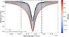 |
Fig. 1 Model fit to the 1142.2 nm refractory Fe I line for star HD 260655. The colored lines represent different synthetic spectra, and the fainter gray lines represent the interpolated grid of spectra that was fit to the data, shown as a black dashed line. The best-fit abundance of [Fe/H] = −0.54 is shown as a darker gray line. It tracks the data over the line region very closely, and is delineated on either side by dashed gray lines. |
4 Radial velocity analysis
For six of the nine planets in our sample, we did not obtain any additional RVs for mass characterization. For these targets, we therefore took the RV semiamplitudes reported in the literature and recalculated our planet masses given our reanalyzed stellar masses calculated in Section 3.1. We similarly recalculated the radii of all nine planets in our sample from Rp/R⋆ values in the literature and our reanalyzed stellar radii. In this section, we detail the process of modeling the RVs obtained for the three remaining targets we selected for an improved mass determination (GJ 1132 b, GJ 1252 b, and LTT 3780 b).
4.1 Radial velocity model
To measure planetary parameters, we modeled all available RV time series for a given star simultaneously. The data are modeled as the sum of Np Keplerian planetary signals, where Np is the number of known planets in the system, and stellar variability. We modeled stellar variability as a Gaussian process (GP; Rasmussen & Williams 2006) for each instrument separately (as our RV time series have been taken at a variety of wavelengths, and stellar variability is inherently chromatic), while sharing multiple hyperparameters between each GP. RV offsets γ were added on a per-instrument basis as well.
We parameterized each Keplerian orbital signal with five parameters: the period of the planet P, the time of inferior conjunction t0, the natural logarithm of RV semiamplitude log K, and ![Mathematical equation: $\[h=\sqrt{e} ~\cos~ \omega\]$](/articles/aa/full_html/2026/05/aa58011-25/aa58011-25-eq3.png) and
and ![Mathematical equation: $\[k=\sqrt{e} ~\sin~ \omega\]$](/articles/aa/full_html/2026/05/aa58011-25/aa58011-25-eq4.png) , where e and ω are the orbital eccentricity and argument of periastron respectively (Lucy & Sweeney 1971). All three planets of interest are expected to be tidally circularized given their short orbital period of < 2 days, and so for these planets we restricted h = k = 0. Our three planets of interest all have extensive transit observations in the literature that provide exceptionally tight constraints on their linear ephemerides. Because the information content on P and T0 is dominated by these transit observations, we did not attempt to measure these parameters directly from the RV data and instead adopted informative priors on P and T0 from the transit analyses (Xue et al. 2024; Kokori et al. 2023; Bonfanti et al. 2024). We adopted uninformative, uniform priors on log K of each planet. Our prior distributions are reported in Tables B.1, B.2, and B.3.
, where e and ω are the orbital eccentricity and argument of periastron respectively (Lucy & Sweeney 1971). All three planets of interest are expected to be tidally circularized given their short orbital period of < 2 days, and so for these planets we restricted h = k = 0. Our three planets of interest all have extensive transit observations in the literature that provide exceptionally tight constraints on their linear ephemerides. Because the information content on P and T0 is dominated by these transit observations, we did not attempt to measure these parameters directly from the RV data and instead adopted informative priors on P and T0 from the transit analyses (Xue et al. 2024; Kokori et al. 2023; Bonfanti et al. 2024). We adopted uninformative, uniform priors on log K of each planet. Our prior distributions are reported in Tables B.1, B.2, and B.3.
Our GP models of stellar activity were computed using the celerite2 package (Foreman-Mackey et al. 2017; Foreman-Mackey 2018). We adopted the SHOTerm kernel, which is a common choice when modeling quasiperiodic RV variability due to active regions on a rotating star (e.g., Krenn et al. 2024; Kroft et al. 2025). The power spectral density of this kernel at a given frequency, S(ω), is given by
![Mathematical equation: $\[S(\omega)=\sqrt{\frac{2}{\pi}} \frac{S_0 \omega_0^4}{\left(\omega^2-\omega_0^2\right)^2+\omega_0^2 \omega^2 / Q^2}\]$](/articles/aa/full_html/2026/05/aa58011-25/aa58011-25-eq5.png) (1)
(1)
for an undamped angular frequency ω0, a quality factor Q, and a scaling factor S0. However, we used the celerite reparameterizations of these hyperparameters, as they make the hyperparameters intuitive and map onto physical stellar parameters better. These reparameterized hyperparameters are the undamped period of the oscillator ρ = 2π/ω0, the damping timescale of the oscillator τ = 2Q/ω0, and the standard deviation of the process (serving as a proxy for the GP amplitude) ![Mathematical equation: $\[\sigma=\sqrt{S_{0} \omega_{0} Q}\]$](/articles/aa/full_html/2026/05/aa58011-25/aa58011-25-eq6.png) . It should be noted that we fit log τ and log σ instead of τ and σ directly. As the oscillation period ρ is directly informed by the rotation period of the star, we adopted priors for the undamped oscillation period of our GP equal to the previously reported rotation periods for each star (obtained from Bonfils et al. 2018, Shporer et al. 2020, and Cloutier et al. 2020 for GJ 1132, GJ 1252, and LTT 3780 respectively). log τ was restricted by a uniform prior to be between log(2) and log(100) times the median of our prior for the rotation period of the star. log σ parameters were given uninformative uniform priors.
. It should be noted that we fit log τ and log σ instead of τ and σ directly. As the oscillation period ρ is directly informed by the rotation period of the star, we adopted priors for the undamped oscillation period of our GP equal to the previously reported rotation periods for each star (obtained from Bonfils et al. 2018, Shporer et al. 2020, and Cloutier et al. 2020 for GJ 1132, GJ 1252, and LTT 3780 respectively). log τ was restricted by a uniform prior to be between log(2) and log(100) times the median of our prior for the rotation period of the star. log σ parameters were given uninformative uniform priors.
Each RV time series was modeled with its own GP; the hyperparameters ρ and log τ were shared between the individual GPs, but log σ was fit separately for each. GJ 1132 and GJ 1252 both have three RV time series (the NIRPS RVs, the archival HARPS RVs, and the HARPS RVs taken simultaneously with NIRPS); due to the large temporal gap between the archival HARPS RVs and the HARPS measurements taken simultaneously with NIRPS, we treated them as two different datasets and instruments for this analysis for the two stars. We fit six RV time series for LTT 3780 (the NIRPS RVs, the CARMENES RVs, the archival HARPS RVs, the HARPS-N RVs, and the MAROON-X RVs, which were split up into the red and blue arms due to their chromatic nature.) All of these time series are described in more detail in Section 2.
We used the emcee package (Foreman-Mackey et al. 2013) to perform Markov chain Monte Carlo (MCMC) sampling of the joint posterior PDFs of our models. We used 64 walkers and run the MCMC for a sufficient number of steps until the chain length is more than 50× the autocorrelation time, indicating the chains are well mixed.
4.2 Results
A table of the priors and posteriors for the RV model for each planetary system can be found in Tables B.1, B.2, and B.3. Phase-folded plots of the planetary signals from each system are shown in Figures 2, 3, and 4; plots of the full RV time series for all three systems are shown in Appendix B.
We obtained final masses of 1.69 ± 0.15 M⊕ and 2.91 ± 0.27 M⊕ for GJ 1132 b and c, respectively. These are both consistent with the most recently reported masses of 1.66 ± 0.19 M⊕ and 2.64 ± 0.44 M⊕ for the two planets, identified by Xue et al. (2024) and Bonfils et al. (2018), but represent significant mass precision improvements (from 9.7σ to 11.3σ for GJ 1132 b and 6σ to 10.8σ for GJ 1132 c.)
We obtained final masses of 1.54 ± 0.18 M⊕ and 6.08 ± 0.86 M⊕ for GJ 1252 b and c, respectively. These are both consistent with the most recently reported masses of 1.32 ± 0.28 M⊕ and 7.4 ± 1.0 values for the two planets, identified in Luque & Pallé (2022) (with GJ 1252 (c)’s previously estimated mass calculated from the reported semiamplitude and period), with GJ 1252 b’s mass precision improving from 4.7σ to 8.6σ, and GJ 1252 (c)’s mass precision remaining mostly unchanged (from 7.4σ to 7.1σ, mostly due to a lower calculated mass.)
We obtained final masses of 2.34 ± 0.10 M⊕ and 7.89 ± 0.26 M⊕ for LTT 3780 b and c, respectively. These are both consistent with the most recently reported masses of 2.46 ± 0.19 M⊕ and ![Mathematical equation: $\[8.04_{-0.48}^{+0.50}\]$](/articles/aa/full_html/2026/05/aa58011-25/aa58011-25-eq7.png) M⊕ for the two planets, reported in Bonfanti et al. (2024), and represent mass precision improvements from 13σ to 23σ for LTT 3780 b and 17σ to 30σ for LTT 3780 c.
M⊕ for the two planets, reported in Bonfanti et al. (2024), and represent mass precision improvements from 13σ to 23σ for LTT 3780 b and 17σ to 30σ for LTT 3780 c.
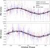 |
Fig. 2 Detrended and phase-folded RV time series of GJ 1132 b (top) and GJ 1132 c (bottom). Different draws of the Keplerian models from our posterior are superimposed in black. The different colored markers correspond to different RV time series. The binned data points are shown as red squares. |
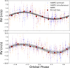 |
Fig. 3 Phase-folded and detrended RV time series of GJ 1252 b (top) and GJ 1252 (c) (bottom). The best-fit Keplerian model is superimposed in black. The different colors and markers correspond to different RV time series. Binned data points are shown as red squares. |
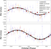 |
Fig. 4 Phase-folded and detrended RV time series of LTT 3780 b (top) and LTT 3780 c (bottom). The best-fit Keplerian model is superimposed in black. The different colors and markers correspond to different RV time series. Binned data points are shown as red squares. |
4.3 The GJ 1252 system, and modeling GJ 1252 (c)
Luque & Pallé (2022) reported the discovery of a second non-transiting planet candidate, GJ 1252 (c), at 17.5 days. The inclusion of additional planets in an RV model can potentially impact the recovered masses of confirmed planets, even if the two planets do not have similar periods (e.g., Almenara et al. 2022). We considered RV models of the GJ 1252 system with the inclusion of one versus two planetary signals, and perform a detailed model comparison between the two.
We modeled the one-planet case (with only GJ 1252 b on a circular orbit) and the two-planet case, which included the planet candidate GJ 1252 (c) on a freely eccentric orbit. These two models included informed stellar activity GPs with the same priors. We report the results of the two GJ 1252 model fits in Table B.2. We note that the data were effectively modeled in both cases. While the two-planet case modeled the data well, we saw no significant 17.5d signal in the residuals of the archival HARPS RVs, as can be seen in Figure 5. We additionally saw no 17.5d signal in the NIRPS RVs, either the raw RVs or the residuals. In addition, the rotation period that both cases independently fit to is 55d, at the 3 : 1 harmonic of the 18.41d period of GJ 1252 (c) identified in the posterior, strongly suggesting that either this signal is not planetary in nature or that the stellar activity GP can effectively model out this signal.
To identify the preferred model, we estimated the Bayesian evidence of our models using the Perrakis estimator (Perrakis et al. 2014). The Perrakis estimator is an estimator of the fully marginalized likelihood (aka the Bayesian evidence) that utilizes the unnormalized posterior PDF from our MCMC sampling as an importance sampler. Assuming that our MCMC sampling has adequately explored the posterior parameter space for each model, the Perrakis estimator can approximate the Bayesian evidence ratio of competing models with a precision of roughly 103 (Nelson et al. 2020), meaning that Bayesian evidence ratios produced by the Perrakis estimator that exceed ~103 are generally considered significant. This method has been commonly used in recent years to estimate Bayesian evidences of RV planetary signals for the purpose of model comparison (e.g., Díaz et al. 2016; Bonomo et al. 2017; Lillo-Box et al. 2020; Suárez Mascareño et al. 2020; Cloutier et al. 2023; Balsalobre-Ruza et al. 2025).
We find that the two-planet model is favored over the one-planet model by Δ ln(Z) = 26.6, which would appear to provide very strong evidence for the two-planet model. However, we reemphasize that our one-planet+GP model does effectively fit the 17.5 day periodicity seen in the GLS of the GJ 1252 RVs such that we do not claim to have evidence that the 17.5-day signal is planetary in nature. We also note that the resulting masses for GJ 1252b from the two models are consistent (i.e., 1.43 ± 0.19 M⊕ and 1.54 ± 0.18 M⊕ for the one- and two-planet models, respectively). Consequently, the results from our forthcoming interior structure analysis are not significantly impacted by our choice of model. We elected to use the GJ 1252 b mass obtained from our two-planet model in subsequent analyses because it is strongly favored by the Bayesian evidence ratio.
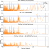 |
Fig. 5 Generalized Lomb–Scargle periodogram of the archival HARPS RVs of GJ 1252. Each panel shows a different step of the one-planet model: the raw RVs (top); the RVs with the maximum a-posteriori (MAP) GJ 1252 b Keplerian model subtracted out (second); the RVs with the MAP stellar activity model subtracted out (third), and the RVs with both the MAP stellar activity model and GJ 1252 b Keplerian model subtracted out (bottom). Red lines corresponding to false alarm probabilities (FAPs) of 1% and 0.1% are overplotted, as are gray lines corresponding to 0.52 d (GJ 1252b period), 17.5d (GJ 1252 (c) period reported in Luque & Pallé 2022), and 64 d (the stellar rotation period reported in Shporer et al. 2020). |
4.4 Mass–radius diagram
Table A.2 details the reanalyzed masses and radii of our entire sample of planets. We have plotted the masses and radii of our planets, with an Earth-like composition curve from Zeng et al. (2019) and composition curves taking into account water dissolution and sequestration (discussed in Section 6.4), in Figure 6.
All nine planets lie above the Earth-like composition curve in mass-radius space, indicating radii larger than expected for Earth-like compositions at their measured masses, and therefore lower bulk densities. We also note that none of our planets lie below this curve, meaning we do not see any super-Mercuries in our sample.
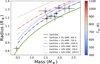 |
Fig. 6 Reanalyzed radii vs. masses of all the planets in our sample. The colors of data points are determined based on equilibrium temperature, according to the colorbar. Several composition curves are overlaid. A curve corresponding to an Earth-like composition from Zeng et al. (2019) is shown as solid green line. Curves corresponding to water mass fractions of 3% (dash-dotted) and 10% (dotted) are shown at 400, 700, and 1000 K, and are linearly interpolated based on the same pretabulated models discussed in Section 6.4. |
5 Determining the core mass fraction
We derived the CMFs of our planets in two different ways for the purpose of comparison. We begun by calculating the CMF of each planet from its measured mass and radius, and assuming that its bulk composition is well-described by just two components: a differentiated iron core beneath a silicate mantle (CMFplanet). Secondly, we calculated the expected CMF of each planet based on the Mg, Si, and Fe abundances of its host star (CMFstar). In calculating CMFstar, we assumed that the refractory abundance ratios of the planets are identical to that of its host star.
Comparing the CMFplanet and CMFstar values for each planet may give us insight into the formation and evolutionary processes of close-in super-Earths around M dwarfs. Specifically, if the planetary and stellar CMF predictions are roughly equal at the population level, then that would imply that the compositions of terrestrial super-Earths around M dwarfs are set by the stellar composition and that no subsequent iron enhancement or depletion processes are affecting these planets’ compositions. If these planets instead tend to exhibit larger CMFs than expected from their host stars, then that would imply a more massive iron core than is expected from formation, and suggests that mantle stripping by giant impacts is a driving process that sets these planets’ compositions (Marcus et al. 2010). Lastly, if these planets tend to exhibit smaller CMFs than expected from their host stars, that would imply either an iron depleted interior or some form of dilution by a low density species (e.g., water). Planet formation models do not predict significant iron depletion of planets (e.g., Scora et al. 2020), as the refractory abundances in FGK stars in the solar neighborhood are largely homogeneous (Brewer et al. 2016; Bedell et al. 2018). In addition, the relevant species found inside terrestrial planets have very similar condensation temperatures (Dorn et al. 2019), and so they should contribute in nearly equal proportions to forming protoplanets. Because of this, if the planets in our sample have smaller CMFs than expected, the assumption of a planet composed entirely of iron and silicates is likely incorrect. Recent theory suggests that super-Earths can sequester water deep inside their cores, inflating their radii, reducing their bulk densities and inferred CMF values compared to when a pure iron core is incorrectly assumed (Luo et al. 2024). However, for planets to have significant amounts of water sequestered inside their cores, the water would have to be accreted early on in the planet formation process. Smaller CMF values than expected would therefore be consistent with water-rich formation around M dwarfs and help constrain the nature of the accretion process.
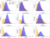 |
Fig. 7 Set of posterior PDFs showing the distributions of CMFplanet, the CMF of the planets as measured from their masses and radii (orange), and CMFstar, the equivalent CMF as inferred from the refractory abundances of their host stars (blue), for each planet. Due to the high uncertainty in abundances for some stars, such as GJ 1252, some draws from the posterior are fit with very low [Fe/H] values and very high [Mg/H] and [Si/H] values, resulting in a very low CMFstar, causing a large amount of posterior draws to converge to CMFstar ≈ 0. |
5.1 Mass- and radius-derived core mass fraction estimates
We used the rocky planet interior structure modeling package exopie (Plotnykov & Valencia 2024) to infer CMFplanet values from the planetary masses and radii reported in Table A.2. exopie is an updated version of the earlier internal structure code SuperEarth (Plotnykov & Valencia 2020). We used exopie to generate forward models of exoplanet radii given an exoplanet mass, CMF, and the molar fraction of silicon in the core and the molar fraction of iron in the mantle, xSi and xFe, which were allowed to vary uniformly between 0 and 0.2. As these planets are very close to their host stars, with Teq > 373 K (the boiling point of water at 1 atm), our models assumed that these planets have no water or significant atmospheres, meaning these models assumed interior compositions that include a primarily iron core and a primarily silicate mantle. These assumptions are appropriate for likely rocky planets below the radius valley (R < 1.6 R⊕, Rogers 2015); as all of our planets have a radius below 1.4 R⊕, this is a safe assumption for our entire sample.
exopie samples the joint prior parameter space on Mp, xSi, xFe, CMF to find the set of planetary parameters that result in a planet whose radius best fits the observed planet radius, assuming realistic mineralogy. The corresponding CMF posterior is our parameter of interest (i.e., CMFplanet). For each planet, we sampled the parameter space with 105 draws to quantify the CMFplanet posterior. The resulting CMFplanet distributions are depicted in Figure 7 and point estimates are reported in Table A.2.
5.2 Stellar abundance-derived core mass fraction estimates
In addition to inferring CMFplanet from the planetary masses and radii, we computed the planetary CMFs that are expected from the refractory abundances of their host stars (i.e., CMFstar). The CMFstar values assume that rocky planets preserve the refractory abundance ratios exhibited in the host stellar photosphere such that discrepancies between CMFplanet and CMFstar can tell us something about the rocky planet formation process.
We used exopie to derive CMFstar from stellar refractory abundances, using an equivalent chemical planetary model to that used in the interior structure modeling presented in Section 5.1. exopie solves for the chemical inventory of a sampled rocky configuration, allowing xSi and xFe to vary between 0 and 0.2 as in Section 5.1, such that the final refractory ratios (Fe/Mg, Fe/Si, Mg/Si) of the planet best match the measured stellar abundance ratios in Table A.1. This calculation is very similar to previous estimates to calculate a CMF from stellar abundances (e.g., Schulze et al. 2021); in fact, when xSi and xFe are set to 0, the equivalent expression for CMFstar is functionally equivalent to that presented in Equation (2) of Schulze et al. (2021), with any differences in estimates due only to the different mineralogy used in exopie versus what is used in that work.
For each star, we drew 104 samples of the refractory abundances of Mg, Si, and Fe from assumed Gaussian distributions set by the mean values and uncertainties identified in Section 3.2 and calculated the corresponding CMFstar with exopie. The resulting CMFstar distributions are included in Figure 7, with point estimates also reported in Table A.2.
6 Discussion
6.1 The CMFplanet and CMFstar distributions are statistically different
We find that for eight of our nine planets in our sample (excepting only L 98-59b), the median values of the posteriors for CMFplanet is lower than the median values for CMFstar. While the large uncertainties in the two CMF distributions make it difficult to draw concrete conclusions for any individual system, our finding that CMFplanet < CMFstar applies to the majority of planets in our sample suggests a clear trend.
We quantified this by estimating the population mean difference between our two CMF estimates, ΔCMF = CMFplanet − CMFstar, through Monte Carlo resampling. To estimate ΔCMF, we sampled draws from the posteriors of CMFplanet and CMFstar for each of our planets. We then calculated the difference between the mean of the CMFplanet draws and the CMFstar draws (which is equivalent to calculating the average of the differences between the two CMF estimates for each planet). We repeated this process 105 times and observed the distribution of ΔCMF draws, which are shown in Figure 8.
We find that 94.7% of ΔCMF draws are below 0, while 5.3% of draws are above 0.95% of ΔCMF draws fall between [−0.224, 0.022]. Because the vast majority of the ΔCMF distribution lies below 0, we interpret this as strong evidence of a systematic offset between our CMFstar and CMFplanet distributions at the population level.
6.2 Possible interpretations of the planetary structure
We have established that the CMFs of hot super-Earths around M dwarfs in our sample are systematically lower than expected if they formed solely from the primordial refractory materials in their host stars. If we continue to assume that these planets are constructed out of solely iron and silicates, then our results would imply that they have significantly less massive iron cores than their host stars’ abundances would suggest. Planet formation models do not predict significant iron depletion of super-Earths (e.g., Scora et al. 2020). This follows from the observational result that the refractory abundances of FGK stars in the solar neighborhood are largely homogeneous (Brewer et al. 2016; Bedell et al. 2018) and because Mg, Si, and Fe all have similar condensation temperatures (Dorn et al. 2019). As these stars aren’t expected to be iron-depleted, and there is a vanishingly small temperature range in a protoplanetary disk where some but not all of these three refractories would have condensed, we do not expect these planets to have formed from iron-depleted material.
If they exist, thick atmospheres on these planets (either hydrogen/helium atmospheres or steam atmospheres) could in theory increase the observed radii of these planets, decreasing their measured densities and thus accounting for this discrepancy. However, as these planets are very hot and relatively small, thick atmospheres do not appear likely on these planets. Hydrogen and helium would be likely to have undergone atmospheric escape, while if a differentiated water atmosphere were to have existed on these planets, their high equilibrium temperatures would have likely led any steam to photodissociate, whereupon the H2 and O2 would likely be lost to space (Schaefer et al. 2016). It should be noted as a caveat that some O2 may be sequestered in this instance; see Schaefer et al. 2016 for a discussion on this focusing on GJ 1132 b specifically. It is also possible that water on these planets may have been converted to hydrogen or sequestered as well, resulting in low atmospheric water mass fractions (WMFs) (Luo et al. 2024; Gupta et al. 2025; Werlen et al. 2025).
Models based on observations of XUV flux from M dwarfs predict that most super-Earths around M dwarfs (including specifically our entire sample of planets) are unlikely to retain significant atmospheres, as well (Pass et al. 2025). Observational evidence supports this too: observations of super-Earths around M dwarfs are unlikely to find significant atmospheres (Kreidberg & Stevenson 2025). In addition, observations attempting to directly constrain the atmospheres of several planets in our sample have been performed, and have found results consistent with no thick atmosphere for GJ 1132 b (Libby-Roberts et al. 2022; May et al. 2023; Bennett et al. 2025; Palle et al. 2025), GJ 1252 b (Crossfield et al. 2022), LTT 3780 b (Allen et al. 2025), GJ 357 b (Adams Redai et al. 2025; Taylor et al. 2025), L 98-59 c (Scarsdale et al. 2024), and LHS 1140 c (Cadieux et al. 2024a; Rochon et al. 2026). L 98-59 b is believed to potentially host a thin secondary atmosphere (Bello-Arufe et al. 2025), and TOI-270 b may host a thin steam atmosphere (Coulombe et al. 2025), but both are likely not thick enough to substantially affect the observed radius of this planet. It therefore seems unlikely that the presence of thick atmospheres is the primary cause of the difference between our CMFplanet and CMFstar distributions.
One alternative explanation is that the interiors of hot super-Earths around M dwarfs are made, in part, of a nonnegligible mass fraction of lower density materials, such as water. The structure models used in Section 5 to calculate the CMFs of our planets do not account for the presence of volatiles, either sequestered or differentiated, and so the presence of volatiles on the planets but not in our models could explain the discrepancy. Geochemical theory suggests that water can be sequestered deep inside the cores and mantles of super-Earths (Luo et al. 2024). Water sequestration can substantially inflate the planetary radius by up to 25% more than it would have without water, in the process deflating the bulk density and thus the inferred CMFplanet (Luo et al. 2024). Our results suggest that hot super-Earths around M dwarfs do harbor nonnegligible WMFs.
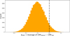 |
Fig. 8 Distribution of ΔCMF draws, as described in Section 6.1. A vertical black line corresponding to ΔCMF = 0 is overplotted. |
6.3 A dearth of super-Mercuries
Super-Mercuries are a proposed class of exoplanet characterized by radii similar to those of super-Earths but with very high densities, requiring CMFs well above that of Earth to explain. We note that none of our targets exhibit a CMFplanet value that exceeds CMFstar. We therefore observe no evidence of iron enhancement in any of our targets, which is the defining characteristic of super-Mercuries. An elevated CMFplanet is an expected outcome of mantle stripping by giant impacts (Marcus et al. 2010), which is believed to have played a key role in the late phases of final assembly of the terrestrial planets in the Solar System (Levison & Agnor 2003; Raymond et al. 2005; Kokubo et al. 2006; Armitage 2020). Our results suggest that giant collisions do not play a key role in the formation of super-Earths around M dwarfs, perhaps owing to their low occurrence rates of cold gas giants (Fulton et al. 2021; Bryant et al. 2023; Pass et al. 2023) that may be needed to perturb planetesimals onto crossing orbits (Chambers & Wetherill 1998).
6.4 Calculating the WMFs of hot super-Earths around M dwarfs
It should be noted that while we calculated WMFs assuming water-rich planets, alternative proposed compositions such as soot planets or other light elements in the core (e.g., Li et al. 2026) may be consistent with the planetary masses and radii reported in this work. However, we reemphasize that we favor the water-rich interpretation of given the wealth of observational evidence for water-rich formation already discussed in Section 1. With the knowledge that the presence of sequestered volatiles inside these planets is possible, we then calculated the planets’ WMFs assuming that the water is either sequestered in the planet core and mantle or fully differentiated.
We obtained our first set of WMF estimates by allowing the water to be sequestered into the planet core and mantle. The partitioning of water depends on the planetary parameters mass, temperature, and compositional mass fractions, and are tabulated using the model presented in Luo et al. (2024). The models define the radius of the planet as the radius of 1 mbar pressure in any steam atmosphere, if it exists. For simplicity, we elected to fix the CMF to an Earth-like value of 0.325 while sampling the mass, Teq, WMF, and (as a dependent variable) radius over the ranges of [0.5, 30] M⊕, [300, 2500] K, [0.01, 0.40], and roughly [0.85, 3] R⊕, respectively. We note that the CMFstar values for all of our target stars are consistent with an Earth-like CMF to <1σ, such that fixing the CMF to CMF⊕ is a reasonable assumption.
We calculated this first set of WMF estimates by interpolating our interior structure model table with 104 samples from the input parameter posteriors. For each of the planets in our sample, we resampled the mass, radius, and Teq from our median values and uncertainties in Table A.2, assuming Gaussian errors. We then performed a piecewise linear interpolation over those three parameters to find the WMF of this realization. All sampled parameters outside of the ranges of planet parameters sampled in the model tabulations were ignored. The resulting WMF posteriors are given in Table 1.
We obtained our second set of WMF estimates by assuming that the planet is fully differentiated with the water layer forming the surface of the planet. While the high equilibrium temperatures of these planets may preclude a surface water layer, we still wished to measure the expected WMFs of these planets with this method as a point of comparison. To calculate this second set of WMF estimates, we used the interior structure modeling code smint (Piaulet et al. 2021; Piaulet-Ghorayeb et al. 2024), which couples an interpolator of planetary structure models of rocky (Zeng et al. 2016) and irradiated ocean worlds (Aguichine et al. 2021) with the MCMC sampler emcee (Foreman-Mackey et al. 2013). These planets are modeled as an iron core, a silicate rock mantle, and a water layer on top. The water layer is expected to be in a vapor/supercritical phase, as all our targets have Teq > 400 K (Aguichine et al. 2021). The planetary radius produced by the models for a given mass and WMF is compared to the observed radius; the mass and irradiation temperatures Tirr are constrained by Gaussian priors from the values found in Tables A.2. The Tirr values are assumed to be equal to the Teq values, which are calculated as if the Bond albedo is 0. To be able to properly compare to our first set of WMF estimates, we fixed the CMF to the same value of 0.325. The resulting WMFs are reported in Table 1.
We find that for nearly every planet in our sample, the resulting WMFs assuming water is sequestered are consistent with 0.01 (the smallest WMF sampled in the pre-tabulated models.) The only planet for which this is not the case is L 98-59b, though it should be noted that due to its small mass, 70% of the sampled parameters were outside of the range of input parameters for the pre-tabulated models, and so were ignored when calculating the posterior. Similarly, we find that the WMFs for the planets in our sample tend to hover around 1–2% if water is differentiated on the surface of the planet. These numbers, while largely not consistent with WMFs of 0, are nevertheless very low.
Recently, Rogers et al. (2025) compared the interior models of Luo et al. (2024) with an observed sample of super-Earths to place upper limits on the WMFs of super-Earths at the population level. In the case of super-Earths without atmospheres or mantle outgassing, they find that super-Earths have no more than 3% WMFs on average.
We find that the WMFs of our sample planets calculated using both methods are largely consistent with this WMF upper limit. We may not necessarily expect water on these planets to be differentiated, and photodissociation or sequestration of this water seems more likely instead (Werlen et al. 2025), but measuring the WMFs of these planets alone does not seem sufficient to distinguish between these two possibilities.
Calculated WMFs.
Comparison with other papers.
6.5 The star-planet compositional connection
Past studies have tried to quantify the relation between the compositions of rocky planets and their host stars (Plotnykov & Valencia 2020; Adibekyan et al. 2021; Schulze et al. 2021; Liu & Ni 2023; Adibekyan et al. 2024; Brinkman et al. 2024, 2025; Plotnykov et al. 2026). These studies have produced a range of different results, in part due to differences in sample selection and methods. For example, Plotnykov & Valencia (2020) found that some planets may be iron-depleted relative to their host stars; Brinkman et al. (2024) identified a relation consistent with one-to-one between planetary and host CMFs, though due to uncertainties in both was unable to draw a conclusive correlation, while Adibekyan et al. (2021) identified a very strong correlation between the planetary and host stellar iron mass fractions. However, all of these studies were primarily based on analysis of planetary systems around FGK stars, with little to no contributions from M dwarfs. In this study, however, we are in a position to compare the star-planet correlations reported for FGK stars to that around M dwarfs.
Several of these studies (Adibekyan et al. 2021, 2024; Brinkman et al. 2024) fit a linear relation between their two CMF estimates (or proxies thereof), which we replicate here for our M dwarf planet sample. To quantify the relation between CMFstar and CMFplanet, we performed a linear fit of the form CMFplanet = mCMFstar + b. We performed a Monte Carlo simulation by directly resampling CMF values from the distributions reported in Table A.2 and shown in Figure 7 104 times and performing an ordinary least-squares (OLS) fit for each realization. We recovered a slope m = 0.0 ± 0.5 and an intercept b = 0.2 ± 0.2. A plot of this fit is shown in Figure 9.
We also performed an independent analysis using orthogonal distance regression (ODR) with SciPy.odr (Virtanen et al. 2020). As the CMFplanet distributions are not Gaussian for many of the stars (being truncated at 0), we repeated the same boot-strapping as before. We recovered a slope of m = 1.9 ± 7.5, and an intercept of b = −0.4 ± 2.2. We note that the slope obtained from ODR is highly unconstrained, likely due to our small sample size, high uncertainties in the two CMF estimates, and lack of planets with very high or very low CMFstar values to leverage the linear fit. We therefore only compared our OLS fit results to the results from other studies. A comparison of the best-fit slopes and the best-fit value of CMFplanet (or a proxy thereof) at a solar CMFstar = 0.3 (the value calculated by exopie at solar abundances) is given in Table 2.
A one-to-one relation between CMFplanet and CMFstar (corresponding to a slope of one) suggests that planets and their host stars have similar compositions. A slope greater than one, meanwhile, suggests that iron-rich stars host planets even further enriched beyond their stellar composition, while a slope of zero would suggest that the iron-to-silicate ratio of the planet is completely uncorrelated with the composition of its host star. Our slope of 0.0 ± 0.5 represents a 2σ departure from the hypothesis that planets and their host stars have equal iron-to-silicate ratios, though the small sample size may make drawing concrete conclusions from this relation difficult.
These results appear to mark a departure from other works performing similar analyses on primarily FGK stars, as well. The slope of the relation between CMFplanet and CMFstar (or proxies thereof) varies significantly across previous analyses of different samples of planet-hosting stars. Adibekyan et al. (2021), Liu & Ni (2023), and Adibekyan et al. (2024) identified very steep slopes, much greater than unity, while Brinkman et al. (2024) and Brinkman et al. (2025) identify slopes of 1.3 ± 1.0, thus finding no strong evidence for a relation between star and planet abundances. We find a similarly weak linear relation to Brinkman et al. (2024) and Brinkman et al. (2025), which is marginally weaker but only at the 1.0σ level. It should be noted that some planets in the sample presented here do appear in Liu & Ni (2023); this work tends to find substantially lower CMF estimates across this shared sample. We chalk this up to the fact that we homogenously reanalyzed stellar masses and radii in this sample, and substantially improved the mass precision for many of the shared targets.
We also note that we recovered substantially lower CMFplanet values than in any of the aforementioned studies. In Table 2, we report the resulting CMFplanet values from the various linear fits, evaluated at the solar CMFstar = 0.3 (equivalently, 0.332 for Fe%star as calculated in Adibekyan et al. 2021). The value of CMFplanet (or a similar proxy) at solar abundance/CMF is not generally reported, and so for papers other than this one it is estimated from plots in the corresponding papers. We find that our OLS fit predicts CMFplanet = 0.19 ± 0.05 at solar CMFstar. This value is in marked contrast to previous analyses for planets around predominantly FGK stars, all of which predict CMFplanet or Fe%planet values of 0.34–0.55 at solar CMFstar. Our result differs from all previous analyses described above by at least 1.5σ, with studies analyzing primarily FGK stars finding substantially higher CMF estimates than the planets around M dwarfs presented in this study. We conclude that close-in super-Earths around M dwarfs show evidence for lower CMFs than around FGK stars, which we interpret as evidence for larger WMFs.
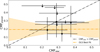 |
Fig. 9 Correlation between CMFplanet and CMFstar for the nine hot super-Earths in our sample. The 95% upper limits are denoted with downward arrows. The line CMFplanet = CMFstar is overplotted as a dash-dotted black line. Our OLS fit with 1σ confidence intervals is shown in orange. The ODR fit is not shown here due to its high uncertainty. |
6.6 Recommending future observing strategies
While the CMFplanet and CMFstar distributions presented in this work are statistically distinct, future studies studying compositions of rocky planets around M dwarfs on a population level may strive to better characterize these parameters. This may be accomplished by either improving mass measurement precisions or by increasing the planet sample size. We calculated the total observing times required for both approaches to identify which is more efficient at improving the characterization of the CMFplanet and CMFstar distributions.
We begun by defining a proxy for the distinctness of these distributions: the difference between the posterior of the mean CMFplanet and CMFstar values in our sample. To derive this value, we resampled the two CMF values of each planet from their posteriors 104 times (c.f., Figure 7) and tracked the mean CMF as a function of the number of planets sampled. The results of this exercise are shown in the upper panel of Figure 10. With our current sample of nine planets, we achieved a 1.6σ difference between our mean CMFplanet and CMFstar distributions. We note, however, that while 1.6σ may not seem like much, we have already shown the two CMF distributions are indeed statistically different.
Next, we calculated the improvement in the mean CMF precisions that are expected to be gained from a hypothetical observing campaign aimed at improving the mass measurements precisions of the nine targets in our sample to 10σ. We assumed that the resulting CMFplanet posteriors have identical means to their current values, but have uncertainties identical to the current uncertainty of the CMFplanet of LTT 3780 b (0.15). We also assumed that the CMFstar distributions would remain unchanged. We then repeated the same resampling process to compute the resulting mean CMFplanet distribution. The results of this calculations are shown in the middle panel of Figure 10. As expected, the assumed 10σ mass measurements improve the CMFplanet precision, which would then be distinguishable from the CMFstar distribution at 2.0σ, compared to the 1.6σ difference achieved with our current sample.
Lastly, we repeated this calculation for a hypothetical observing campaign that increases the size of the planet sample with ~5σ mass measurements precision (roughly the lowest mass precision in our current sample). We adopted our mean CMF distributions with our current sample size of nine and iteratively added new planets assuming that they follow the current CMFplanet distribution. For each added planet, we set its CMFstar distribution to the CMFstar distribution from Table A.2 of that system. We also assumed these new planets have CMFplanet posteriors sampled from a truncated Gaussian distribution, with a mean equal to the CMFplanet mean of the same planet but with an uncertainty of 0.22, as this value is roughly equal to the CMFplanet uncertainties of GJ 357 b and L 98-59 b, the two targets in our sample with ~5σ mass precisions. We then repeated the same resampling process as before to compute the mean CMF distributions as a function of the number of planets. The results of this exercise are shown in the lower panel of Figure 10. We find that to match the 2.0σ difference between our mean CMFplanet and CMFstar distributions, ten new targets with 5σ masses are needed.
Given these two possible scenarios, we calculated the strategy that required fewer RV observations and can therefore be completed more efficiently. We used the prescription in Cloutier et al. (2018) to calculate the precision in planetary RV semi-amplitudes given the precision of RV observations (including RV jitter from residual systematics and stellar activity)2,
![Mathematical equation: $\[N_{R V}=3\left(\frac{\sigma_{\mathrm{eff}}}{\sigma_{\mathrm{K}}}\right)^2\]$](/articles/aa/full_html/2026/05/aa58011-25/aa58011-25-eq11.png) (2)
(2)
where σeff is the effective RV uncertainty of the observations and σK is the goal semiamplitude uncertainty. We assumed fiducial values of σRV = 2.5 m/s (approximately the RV uncertainty for GJ 1132, the target in our sample with the lowest NIRPS RV precision), and assumed a fixed semiamplitude of K = 3 m/s for each new planet. We further assumed that any observing campaign focused on improving mass precisions of the existing sample would seek to improve the mass precision of all targets in this sample that do not already have a ~10σ mass detection (i.e., GJ 357 b, HD 260655 b, L 98-59 b, and TOI-270 b). With the fiducial input values described above, improving the mass precisions of these four targets to 10σ would require approximately 510, 410, 5900, and 360 RVs respectively. We then repeated this calculation for the alternative observing strategy of targeting ten planets with 5σ mass precisions. We find that 5σ masses can be achieved with roughly 52 RVs for each planet, meaning increasing the size of this sample by nine would take roughly 520 total RVs, far smaller than the total number of RVs necessary to improve the mass precision of even three of the four aforementioned targets (1280 RVs). It is clear that future observations aimed at improving the statistical significance of the conclusions we drew here would be far better served by increasing the sample size of hot super-Earths around M dwarfs with precisions of roughly 5σ rather than conducting intensive RV follow-up to improve the mass precision of existing targets to ~10σ.
 |
Fig. 10 Distributions of the mean CMFplanet and CMFstar values as a function of the number of planets, for our current sample (top), for an observation campaign focused on improving the masses of planets already in our current sample (middle), and for an observation campaign focused on increasing the size of our sample (bottom). The dashed lines represent the median values of our CMF distributions, while the shaded regions represent the 1σ upper and lower regions. |
7 Conclusions
We presented the first results from the CMF subprogram within the NIRPS GTO program. We presented data from the NIRPS and HARPS spectrographs measuring precise RVs of three M dwarfs hosting hot super-Earths, GJ 1132, GJ 1252, and LTT 3780, which substantially improve their mass measurement precisions to ~10σ. We also presented measurements of the stellar abundances of the refractory elements Mg, Si, Fe, and in some cases, Ti, using spectral synthesis methods. We measured the abundances for the three aforementioned M dwarfs plus five other M dwarfs hosting hot super-Earths (i.e., GJ 357, HD 260655, L 98-59, LHS 1140, and TOI-270). We calculated the core mass fractions of all nine planets from their masses and radii (CMFplanet) and the equivalent CMFs inferred from the elemental abundances of their host stars (CMFstar). Our main findings are summarized below:
We recovered planetary CMFplanet values to a precision of 12–15% for our three targets with intensive RV follow-up with NIRPS and HARPS. We recovered a typical CMFplanet precision of ~20% for the five remaining targets. We also recovered CMFstar values implied by our host stellar abundances to a typical precision of ~10%;
Eight of our nine target planets have smaller CMFs than expected from their host star abundances. We showed that this result cannot be attributed to random chance. We do not see strong evidence that the host star abundances track the planetary CMFs for hot super-Earths around M dwarfs;
The significant discrepancy between the CMFplanet and CMFstar distributions suggests that these planets have a significant mass fraction of water. This water is likely sequestered in the planetary interior and not differentiated on the surface, because the equilibrium temperatures of the planets that are expected to vaporize any surface water are high;
We calculated the WMFs necessary to produce these discrepancies assuming that the water is either sequestered or fully differentiated. The WMFs needed to reconcile our observed CMFplanet-CMFstar discrepancy is ~1% regardless of whether the water is sequestered or differentiated;
None of our planets show evidence for having a larger CMFplanet than the CMFstar expected from the stellar abundances. This lack of super-Mercuries in our sample suggests that these planets may be rare around M dwarfs, although the small sample size limits the inferences that can be made about their occurrence rates or formation mechanisms;
We recommend that future observing campaigns seeking to validate the results of our study focus on increasing the sample size of planets with ~5σ mass precisions and do not try to obtain ultra-precise mass measurements of the nine planets in our current sample.
Acknowledgements
This publication makes use of The Data & Analysis Center for Exoplanets (DACE), which is a facility based at the University of Geneva dedicated to extrasolar planets data visualization, exchange, and analysis. DW thanks Alison Sills for their scientific discussions that improved the quality of the statistical analysis, and Bennett Skinner for their scientific discussions regarding interior structure models. RC acknowledges the support of the Natural Sciences and Engineering Research Council of Canada (NSERC). CC, AL, ÉA, FBa, BB, NJC, RD, LMa, RA, LB, AD-B, LD, PLam, OL, LMo, TV & JPW acknowledge the financial support of the FRQ-NT through the Centre de recherche en astrophysique du Québec as well as the support from the Trottier Family Foundation and the Trottier Institute for Research on Exoplanets. AL acknowledges support from the Fonds de recherche du Québec (FRQ) – Secteur Nature et technologies under file #349961. AC, XB, XDe, TF & VY acknowledge funding from the French ANR under contract number ANR24CE493397 (ORVET), and the French National Research Agency in the framework of the Investissements d’Avenir program (ANR-15-IDEX-02), through the funding of the “Origin of Life” project of the Grenoble-Alpes University. ÉA, FBa, RD & LMa acknowledges support from Canada Foundation for Innovation (CFI) program, the Université de Montréal and Université Laval, the Canada Economic Development (CED) program and the Ministere of Economy, Innovation and Energy (MEIE). SCB, EC, NCS, ED-M, JGd & ARCS acknowledge the support from FCT – Fundação para a Ciência e a Tecnologia through national funds by these grants: UIDB/04434/2020, UIDP/04434/2020. SCB acknowledges the support from Fundação para a Ciência e Tecnologia (FCT) in the form of a work contract through the Scientific Employment Incentive program with reference 2023.06687.CEECIND and DOI 10.54499/2023.06687.CEECIND/CP2839/CT0002. NBC acknowledges support from an NSERC Discovery Grant, a Canada Research Chair, and an Arthur B. McDonald Fellowship, and thanks the Trottier Space Institute for its financial support and dynamic intellectual environment. XDu acknowledges the support from the European Research Council (ERC) under the European Union’s Horizon 2020 research and innovation programme (grant agreement SCORE No 851555) and from the Swiss National Science Foundation under the grant SPECTRE (No. 200021_215200). This work has been carried out within the framework of the NCCR PlanetS supported by the Swiss National Science Foundation under grants 51NF40_182901 and 51NF40_205606. DE acknowledge support from the Swiss National Science Foundation for project 200021_200726. The authors acknowledge the financial support of the SNSF. JIGH, ASM, RRe, NN & AKS acknowledge financial support from the Spanish Ministry of Science, Innovation and Universities (MICIU) projects PID2020-117493GB-I00 and PID2023-149982NB-I00. The Board of Observational and Instrumental Astronomy (NAOS) at the Federal University of Rio Grande do Norte’s research activities are supported by continuous grants from the Brazilian funding agency CNPq. This study was partially funded by the Coordenação de Aperfeiçoamento de Pessoal de Nível Superior—Brasil (CAPES) — Finance Code 001 and the CAPES-Print program. ICL acknowledges CNPq research fellowships (Grant No. 313103/2022-4). BLCM acknowledge CAPES postdoctoral fellowships. BLCM acknowledges CNPq research fellowships (Grant No. 305804/2022-7). JRM acknowledges CNPq research fellowships (Grant No. 308928/2019-9). CMo acknowledges the funding from the Swiss National Science Foundation under grant 200021_204847 “PlanetsInTime”. Co-funded by the European Union (ERC, FIERCE, 101052347). Views and opinions expressed are however those of the author(s) only and do not necessarily reflect those of the European Union or the European Research Council. Neither the European Union nor the granting authority can be held responsible for them. GAW is supported by a Discovery Grant from the Natural Sciences and Engineering Research Council (NSERC) of Canada. RA acknowledges the Swiss National Science Foundation (SNSF) support under the Post-Doc Mobility grant P500PT_222212 and the support of the Institut Trottier de Recherche sur les Exoplanètes (IREx). LB acknowledges the support of the Natural Sciences and Engineering Research Council of Canada (NSERC). This project has received funding from the European Research Council (ERC) under the European Union’s Horizon 2020 research and innovation programme (project SPICE DUNE, grant agreement No 947634). This material reflects only the authors’ views and the Commission is not liable for any use that may be made of the information contained therein. LD acknowledges the support of the Natural Sciences and Engineering Research Council of Canada (NSERC) and from the Fonds de recherche du Québec (FRQ) – Secteur Nature et technologies. ED-M further acknowledges the support from FCT through Stimulus FCT contract 2021.01294.CEECIND. ED-M acknowledges the support by the Ramón y Cajal contract RyC2022-035854-I funded by MICIU/AEI/10.13039/501100011033 and by ESF+. CD acknowledges support from the Swiss National Science Foundation under grant TMSGI2_211313. This work has been carried out in parts within the framework of the NCCR PlanetS supported by the Swiss National Science Foundation under grant 51NF40_205606. FG acknowledges support from the Fonds de recherche du Québec (FRQ) – Secteur Nature et technologies under file #350366. This work was supported by grants from eSSENCE (grant number eSSENCE@LU 9:3), the Swedish National Research Council (project number 2023 05307), The Crafoord foundation and the Royal Physiographic Society of Lund, through The Fund of the Walter Gyllenberg Foundation." LMo acknowledges the support of the Natural Sciences and Engineering Research Council of Canada (NSERC), [funding reference number 589653]. KAM acknowledges support from the Swiss National Science Foundation (SNSF) under the Postdoc Mobility grant P500PT_230225. NN acknowledges financial support by Light Bridges S.L, Las Palmas de Gran Canaria. NN acknowledges funding from Light Bridges for the Doctoral Thesis “Habitable Earth-like planets with ESPRESSO and NIRPS”, in cooperation with the Instituto de Astrofísica de Canarias, and the use of Indefeasible Computer Rights (ICR) being commissioned at the ASTRO POC project in the Island of Tenerife, Canary Islands (Spain). The ICR-ASTRONOMY used for his research was provided by Light Bridges in cooperation with Hewlett Packard Enterprise (HPE). CP acknowledges support from the NSERC Vanier scholarship, and the Trottier Family Foundation. CP also acknowledges support from the E. Margaret Burbidge Prize Postdoctoral Fellowship from the Brinson Foundation. ARCS acknowledges the support from Fundaçao para a Ciência e a Tecnologia (FCT) through the fellowship 2021.07856.BD. AKS acknowledges financial support from La Caixa Foundation (ID 100010434) under the grant LCF/BQ/DI23/11990071. TV acknowledges support from the Fonds de recherche du Québec (FRQ) – Secteur Nature et technologies under file #320056.
References
- Adams Redai, J., Wogan, N., Wallack, N. L., et al. 2025, AJ, 170, 219 [Google Scholar]
- Adibekyan, V., Dorn, C., Sousa, S. G., et al. 2021, Science, 374, 330 [NASA ADS] [CrossRef] [Google Scholar]
- Adibekyan, V., Deal, M., Dorn, C., et al. 2024, A&A, 692, A67 [NASA ADS] [CrossRef] [EDP Sciences] [Google Scholar]
- Aguichine, A., Mousis, O., Deleuil, M., & Marcq, E. 2021, ApJ, 914, 84 [NASA ADS] [CrossRef] [Google Scholar]
- Allen, N. H., Espinoza, N., Diamond-Lowe, H., et al. 2025, AJ, 170, 240 [Google Scholar]
- Almenara, J. M., Bonfils, X., Otegi, J. F., et al. 2022, A&A, 665, A91 [NASA ADS] [CrossRef] [EDP Sciences] [Google Scholar]
- Armitage, P. J. 2020, Astrophysics of Planet Formation, 2nd edn. [Google Scholar]
- Artigau, É., Cadieux, C., Cook, N. J., et al. 2022, AJ, 164, 84 [NASA ADS] [CrossRef] [Google Scholar]
- Artigau, É., Bouchy, F., Doyon, R., et al. 2024, SPIE Conf. Ser., 13096, 130960C [Google Scholar]
- Asplund, M., Grevesse, N., Sauval, A. J., & Scott, P. 2009, ARA&A, 47, 481 [CrossRef] [Google Scholar]
- Balsalobre-Ruza, O., Lillo-Box, J., Silva, A. M., et al. 2025, A&A, 694, A15 [NASA ADS] [CrossRef] [EDP Sciences] [Google Scholar]
- Bedell, M., Bean, J. L., Meléndez, J., et al. 2018, ApJ, 865, 68 [Google Scholar]
- Behmard, A., Brinkman, C. L., Hattori, S., Rubenzahl, R. A., & Bedell, M. 2025, AJ, 170, 282 [Google Scholar]
- Bello-Arufe, A., Damiano, M., Bennett, K. A., et al. 2025, ApJ, 980, L26 [Google Scholar]
- Bennett, K. A., MacDonald, R. J., Peacock, S., et al. 2025, AJ, 170, 205 [Google Scholar]
- Benz, W., Broeg, C., Fortier, A., et al. 2021, Exp. Astron., 51, 109 [Google Scholar]
- Berta-Thompson, Z. K., Irwin, J., Charbonneau, D., et al. 2015, Nature, 527, 204 [Google Scholar]
- Blanco-Cuaresma, S. 2019, MNRAS, 486, 2075 [Google Scholar]
- Blanco-Cuaresma, S., Soubiran, C., Heiter, U., & Jofré, P. 2014, A&A, 569, A111 [CrossRef] [EDP Sciences] [Google Scholar]
- Bonfanti, A., Brady, M., Wilson, T. G., et al. 2024, A&A, 682, A66 [NASA ADS] [CrossRef] [EDP Sciences] [Google Scholar]
- Bonfils, X., Almenara, J. M., Cloutier, R., et al. 2018, A&A, 618, A142 [NASA ADS] [CrossRef] [EDP Sciences] [Google Scholar]
- Bonomo, A. S., Desidera, S., Benatti, S., et al. 2017, A&A, 602, A107 [NASA ADS] [CrossRef] [EDP Sciences] [Google Scholar]
- Bouchy, F., Doyon, R., Pepe, F., et al. 2025, A&A, 700, A10 [NASA ADS] [CrossRef] [EDP Sciences] [Google Scholar]
- Brewer, J. M., Fischer, D. A., Valenti, J. A., & Piskunov, N. 2016, ApJS, 225, 32 [Google Scholar]
- Brinkman, C. L., Polanski, A. S., Huber, D., et al. 2024, AJ, 168, 281 [Google Scholar]
- Brinkman, C. L., Weiss, L. M., Huber, D., et al. 2025, AJ, 170, 109 [Google Scholar]
- Bryant, E. M., Bayliss, D., & Van Eylen, V. 2023, MNRAS, 521, 3663 [CrossRef] [Google Scholar]
- Burn, R., Schlecker, M., Mordasini, C., et al. 2021, A&A, 656, A72 [NASA ADS] [CrossRef] [EDP Sciences] [Google Scholar]
- Burt, J. A., Zellem, R. T., Ciardi, D. R., et al. 2025, AJ, 170, 216 [Google Scholar]
- Cadieux, C., Doyon, R., MacDonald, R. J., et al. 2024a, ApJ, 970, L2 [NASA ADS] [CrossRef] [Google Scholar]
- Cadieux, C., Plotnykov, M., Doyon, R., et al. 2024b, ApJ, 960, L3 [NASA ADS] [CrossRef] [Google Scholar]
- Cadieux, C., L’Heureux, A., Piaulet-Ghorayeb, C., et al. 2025, AJ, 170, 154 [Google Scholar]
- Chambers, J. E., & Wetherill, G. W. 1998, Icarus, 136, 304 [NASA ADS] [CrossRef] [Google Scholar]
- Cherubim, C., Cloutier, R., Charbonneau, D., et al. 2023, AJ, 165, 167 [NASA ADS] [CrossRef] [Google Scholar]
- Cloutier, R., & Menou, K. 2020, AJ, 159, 211 [NASA ADS] [CrossRef] [Google Scholar]
- Cloutier, R., Doyon, R., Bouchy, F., & Hébrard, G. 2018, AJ, 156, 82 [NASA ADS] [CrossRef] [Google Scholar]
- Cloutier, R., Astudillo-Defru, N., Bonfils, X., et al. 2019, A&A, 629, A111 [NASA ADS] [CrossRef] [EDP Sciences] [Google Scholar]
- Cloutier, R., Eastman, J. D., Rodriguez, J. E., et al. 2020, AJ, 160, 3 [Google Scholar]
- Cloutier, R., Greklek-McKeon, M., Wurmser, S., et al. 2023, MNRAS, 527, 5464 [CrossRef] [Google Scholar]
- Cook, N. J., Artigau, É., Doyon, R., et al. 2022, PASP, 134, 114509 [NASA ADS] [CrossRef] [Google Scholar]
- Cosentino, R., Lovis, C., Pepe, F., et al. 2012, SPIE Conf. Ser., 8446, 84461V [Google Scholar]
- Coulombe, L.-P., Benneke, B., Krissansen-Totton, J., et al. 2025, AJ, 170, 226 [Google Scholar]
- Crossfield, I. J. M., Malik, M., Hill, M. L., et al. 2022, ApJ, 937, L17 [NASA ADS] [CrossRef] [Google Scholar]
- Demangeon, O. D. S., Zapatero Osorio, M. R., Alibert, Y., et al. 2021, A&A, 653, A41 [NASA ADS] [CrossRef] [EDP Sciences] [Google Scholar]
- Diamond-Lowe, H., Kreidberg, L., Harman, C. E., et al. 2022, AJ, 164, 172 [NASA ADS] [CrossRef] [Google Scholar]
- Díaz, R. F., Ségransan, D., Udry, S., et al. 2016, A&A, 585, A134 [Google Scholar]
- Dittmann, J. A., Irwin, J. M., Charbonneau, D., et al. 2017, Nature, 544, 333 [NASA ADS] [CrossRef] [Google Scholar]
- Donati, J. F., Kouach, D., Moutou, C., et al. 2020, MNRAS, 498, 5684 [Google Scholar]
- Dorn, C., Khan, A., Heng, K., et al. 2015, A&A, 577, A83 [NASA ADS] [CrossRef] [EDP Sciences] [Google Scholar]
- Dorn, C., Hinkel, N. R., & Venturini, J. 2017a, A&A, 597, A38 [NASA ADS] [CrossRef] [EDP Sciences] [Google Scholar]
- Dorn, C., Venturini, J., Khan, A., et al. 2017b, A&A, 597, A37 [NASA ADS] [CrossRef] [EDP Sciences] [Google Scholar]
- Dorn, C., Harrison, J. H. D., Bonsor, A., & Hands, T. O. 2019, MNRAS, 484, 712 [Google Scholar]
- Foreman-Mackey, D. 2018, RNAAS, 2, 31 [NASA ADS] [Google Scholar]
- Foreman-Mackey, D., Hogg, D. W., Lang, D., & Goodman, J. 2013, PASP, 125, 306 [Google Scholar]
- Foreman-Mackey, D., Agol, E., Ambikasaran, S., & Angus, R. 2017, AJ, 154, 220 [Google Scholar]
- Fulton, B. J., Rosenthal, L. J., Hirsch, L. A., et al. 2021, ApJS, 255, 14 [NASA ADS] [CrossRef] [Google Scholar]
- Gaia Collaboration (Vallenari, A., et al.) 2023, A&A, 674, A1 [NASA ADS] [CrossRef] [EDP Sciences] [Google Scholar]
- Gaidos, E., Ali, A., Kraus, A. L., & Rowe, J. F. 2024, MNRAS, 534, 3277 [Google Scholar]
- Gromek, N. 2025, Master’s thesis, McMaster University, Canada [Google Scholar]
- Günther, M. N., Pozuelos, F. J., Dittmann, J. A., et al. 2019, Nat. Astron., 3, 1099 [Google Scholar]
- Gupta, A., Luo, H., Deng, J., & Burrows, A. 2025, arXiv e-prints [arXiv:2510.24956] [Google Scholar]
- Gustafsson, B., Edvardsson, B., Eriksson, K., et al. 2008, A&A, 486, 951 [NASA ADS] [CrossRef] [EDP Sciences] [Google Scholar]
- Hejazi, N., Crossfield, I. J. M., Nordlander, T., et al. 2023, ApJ, 949, 79 [CrossRef] [Google Scholar]
- Hinkel, N. R., Young, P. A., & Wheeler, III, C. H. 2022, AJ, 164, 256 [Google Scholar]
- Ho, C. S. K., Rogers, J. G., Van Eylen, V., Owen, J. E., & Schlichting, H. E. 2024, MNRAS, 531, 3698 [NASA ADS] [CrossRef] [Google Scholar]
- Irwin, J. M., Berta-Thompson, Z. K., Charbonneau, D., et al. 2015, in Cambridge Workshop on Cool Stars, Stellar Systems, and the Sun, 18, 18th Cambridge Workshop on Cool Stars, Stellar Systems, and the Sun, eds. G. T. van Belle, & H. C. Harris, 767 [Google Scholar]
- Jahandar, F., Doyon, R., Artigau, É., et al. 2024, ApJ, 966, 56 [CrossRef] [Google Scholar]
- Jahandar, F., Doyon, R., Artigau, É., et al. 2025, ApJ, 978, 154 [Google Scholar]
- Kaye, L., Vissapragada, S., Günther, M. N., et al. 2022, MNRAS, 510, 5464 [NASA ADS] [CrossRef] [Google Scholar]
- Kokori, A., Tsiaras, A., Edwards, B., et al. 2023, ApJS, 265, 4 [NASA ADS] [CrossRef] [Google Scholar]
- Kokubo, E., Kominami, J., & Ida, S. 2006, ApJ, 642, 1131 [Google Scholar]
- Kostov, V. B., Schlieder, J. E., Barclay, T., et al. 2019, AJ, 158, 32 [Google Scholar]
- Kreidberg, L., & Stevenson, K. B. 2025, PNAS, 122, e2416190122 [Google Scholar]
- Krenn, A. F., Kubyshkina, D., Fossati, L., et al. 2024, A&A, 686, A301 [NASA ADS] [CrossRef] [EDP Sciences] [Google Scholar]
- Kroft, M. A., Beatty, T. G., Crossfield, I. J. M., et al. 2025, AJ, 170, 150 [Google Scholar]
- Kupka, F., Dubernet, M. L., & VAMDC Collaboration. 2011, Baltic Astron., 20, 503 [Google Scholar]
- Levison, H. F., & Agnor, C. 2003, AJ, 125, 2692 [NASA ADS] [CrossRef] [Google Scholar]
- Li, J., Bergin, E. A., Hirschmann, M. M., et al. 2026, ApJ, 997, L29 [Google Scholar]
- Lillo-Box, J., Figueira, P., Leleu, A., et al. 2020, A&A, 642, A121 [NASA ADS] [CrossRef] [EDP Sciences] [Google Scholar]
- Libby-Roberts, J. E., Berta-Thompson, Z. K., Diamond-Lowe, H., et al. 2022, AJ, 164, 59 [NASA ADS] [CrossRef] [Google Scholar]
- Liu, Z., & Ni, D. 2023, A&A, 674, A137 [NASA ADS] [CrossRef] [EDP Sciences] [Google Scholar]
- Lopez, E. D. 2017, MNRAS, 472, 245 [NASA ADS] [CrossRef] [Google Scholar]
- Lucy, L. B., & Sweeney, M. A. 1971, AJ, 76, 544 [NASA ADS] [CrossRef] [Google Scholar]
- Luo, H., Dorn, C., & Deng, J. 2024, Nat. Astron., 8, 1399 [Google Scholar]
- Luque, R., Fulton, B. J., Kunimoto, M., et al. 2022, A&A, 664, A199 [NASA ADS] [CrossRef] [EDP Sciences] [Google Scholar]
- Luque, R., & Pallé, E. 2022, Science, 377, 1211 [NASA ADS] [CrossRef] [Google Scholar]
- Luque, R., Pallé, E., Kossakowski, D., et al. 2019, A&A, 628, A39 [NASA ADS] [CrossRef] [EDP Sciences] [Google Scholar]
- Mahadevan, S., Ramsey, L. W., Terrien, R., et al. 2014, SPIE Conf. Ser., 9147, 91471G [Google Scholar]
- Mann, A. W., Feiden, G. A., Gaidos, E., Boyajian, T., & von Braun, K. 2015, ApJ, 804, 64 [Google Scholar]
- Mann, A. W., Dupuy, T., Kraus, A. L., et al. 2019, ApJ, 871, 63 [Google Scholar]
- Marcus, R. A., Sasselov, D., Hernquist, L., & Stewart, S. T. 2010, ApJ, 712, L73 [Google Scholar]
- Marfil, E., Tabernero, H. M., Montes, D., et al. 2021, A&A, 656, A162 [NASA ADS] [CrossRef] [EDP Sciences] [Google Scholar]
- May, E. M., MacDonald, R. J., Bennett, K. A., et al. 2023, ApJ, 959, L9 [CrossRef] [Google Scholar]
- Mayor, M., Pepe, F., Queloz, D., et al. 2003, Messenger, 114, 20 [Google Scholar]
- Miguel, Y., Cridland, A., Ormel, C. W., Fortney, J. J., & Ida, S. 2020, MNRAS, 491, 1998 [NASA ADS] [Google Scholar]
- Nelson, B. E., Ford, E. B., Buchner, J., et al. 2020, AJ, 159, 73 [Google Scholar]
- Nowak, G., Luque, R., Parviainen, H., et al. 2020, A&A, 642, A173 [NASA ADS] [CrossRef] [EDP Sciences] [Google Scholar]
- Oddo, D., Dragomir, D., Brandeker, A., et al. 2023, AJ, 165, 134 [NASA ADS] [CrossRef] [Google Scholar]
- Otegi, J. F., Dorn, C., Helled, R., et al. 2020, A&A, 640, A135 [NASA ADS] [CrossRef] [EDP Sciences] [Google Scholar]
- Owen, J. E., & Wu, Y. 2017, ApJ, 847, 29 [Google Scholar]
- Palle, E., Yan, F., Morello, G., et al. 2025, A&A, 697, A31 [NASA ADS] [CrossRef] [EDP Sciences] [Google Scholar]
- Parc, L., Bouchy, F., Venturini, J., Dorn, C., & Helled, R. 2024, A&A, 688, A59 [NASA ADS] [CrossRef] [EDP Sciences] [Google Scholar]
- Pass, E. K., Winters, J. G., Charbonneau, D., et al. 2023, AJ, 166, 11 [NASA ADS] [CrossRef] [Google Scholar]
- Pass, E. K., Charbonneau, D., & Vanderburg, A. 2025, ApJ, 986, L3 [Google Scholar]
- Passegger, V. M., Bello-García, A., Ordieres-Meré, J., et al. 2022, A&A, 658, A194 [NASA ADS] [CrossRef] [EDP Sciences] [Google Scholar]
- Pepe, F., Cristiani, S., Rebolo, R., et al. 2021, A&A, 645, A96 [NASA ADS] [CrossRef] [EDP Sciences] [Google Scholar]
- Perrakis, K., Ntzoufras, I., & Tsionas, E. G. 2014, Computat. Statist. Data Anal., 77, 54 [CrossRef] [Google Scholar]
- Piaulet, C., Benneke, B., Rubenzahl, R. A., et al. 2021, AJ, 161, 70 [NASA ADS] [CrossRef] [Google Scholar]
- Piaulet, C., Benneke, B., Almenara, J. M., et al. 2023, Nat. Astron., 7, 206 [Google Scholar]
- Piaulet-Ghorayeb, C., Benneke, B., Radica, M., et al. 2024, ApJ, 974, L10 [NASA ADS] [CrossRef] [Google Scholar]
- Plez, B. 2012, Turbospectrum: Code for spectral synthesis, Astrophysics Source Code Library [record ascl:1205.004] [Google Scholar]
- Plotnykov, M., & Valencia, D. 2020, MNRAS, 499, 932 [CrossRef] [Google Scholar]
- Plotnykov, M., & Valencia, D. 2024, MNRAS, 530, 3488 [Google Scholar]
- Plotnykov, M., Valencia, D., Ross, A., Reggiani, H., & Schlaufman, K. C. 2026, ApJ, 997, 253 [Google Scholar]
- Rasmussen, C. E., & Williams, C. K. I. 2006, Gaussian Processes for Machine Learning [Google Scholar]
- Raymond, S. N., Quinn, T., & Lunine, J. I. 2005, ApJ, 632, 670 [NASA ADS] [CrossRef] [Google Scholar]
- Rochon, A., ArtigauÉ., Weisserman, D., et al. 2026, ApJ, 998, L39 [Google Scholar]
- Rogers, J. G., Dorn, C., Aditya Raj, V., Schlichting, H. E., & Young, E. D. 2025, ApJ, 979, 79 [Google Scholar]
- Rogers, L. A. 2015, ApJ, 801, 41 [Google Scholar]
- Santos, N. C., Adibekyan, V., Mordasini, C., et al. 2015, A&A, 580, L13 [NASA ADS] [CrossRef] [EDP Sciences] [Google Scholar]
- Santos, N. C., Adibekyan, V., Dorn, C., et al. 2017, A&A, 608, A94 [NASA ADS] [CrossRef] [EDP Sciences] [Google Scholar]
- Sarmento, P., Rojas-Ayala, B., Delgado Mena, E., & Blanco-Cuaresma, S. 2021, A&A, 649, A147 [NASA ADS] [CrossRef] [EDP Sciences] [Google Scholar]
- Scarsdale, N., Wogan, N., Wakeford, H. R., et al. 2024, AJ, 168, 276 [Google Scholar]
- Schaefer, L., Wordsworth, R. D., Berta-Thompson, Z., & Sasselov, D. 2016, ApJ, 829, 63 [NASA ADS] [CrossRef] [Google Scholar]
- Schulze, J. G., Wang, J., Johnson, J. A., et al. 2021, Planet. Sci. J., 2, 113 [NASA ADS] [CrossRef] [Google Scholar]
- Schweitzer, A., Passegger, V. M., Cifuentes, C., et al. 2019, A&A, 625, A68 [NASA ADS] [CrossRef] [EDP Sciences] [Google Scholar]
- Scora, J., Valencia, D., Morbidelli, A., & Jacobson, S. 2020, MNRAS, 493, 4910 [CrossRef] [Google Scholar]
- Seifahrt, A., Stürmer, J., Bean, J. L., & Schwab, C. 2018, SPIE Conf. Ser., 10702, 107026D [NASA ADS] [Google Scholar]
- Shporer, A., Collins, K. A., Astudillo-Defru, N., et al. 2020, ApJ, 890, L7 [Google Scholar]
- Skrutskie, M. F., Cutri, R. M., Stiening, R., et al. 2006, AJ, 131, 1163 [NASA ADS] [CrossRef] [Google Scholar]
- Souto, D., Cunha, K., García-Hernández, D. A., et al. 2017, ApJ, 835, 239 [Google Scholar]
- Suárez Mascareño, A., Faria, J. P., Figueira, P., et al. 2020, A&A, 639, A77 [Google Scholar]
- Tamura, M., Suto, H., Nishikawa, J., et al. 2012, SPIE Conf. Ser., 8446, 84461T [NASA ADS] [Google Scholar]
- Taylor, J., Radica, M., Chatterjee, R. D., et al. 2025, MNRAS, 540, 3677 [Google Scholar]
- Trifonov, T., Caballero, J. A., Morales, J. C., et al. 2021, Science, 371, 1038 [Google Scholar]
- Unterborn, C. T., Desch, S. J., Hinkel, N. R., & Lorenzo, A. 2018, Nat. Astron., 2, 297 [NASA ADS] [CrossRef] [Google Scholar]
- Unterborn, C. T., Desch, S. J., Haldemann, J., et al. 2023, ApJ, 944, 42 [Google Scholar]
- Van Eylen, V., Astudillo-Defru, N., Bonfils, X., et al. 2021, MNRAS, 507, 2154 [NASA ADS] [Google Scholar]
- Venturini, J., Ronco, M. P., Guilera, O. M., et al. 2024, A&A, 686, L9 [NASA ADS] [CrossRef] [EDP Sciences] [Google Scholar]
- Virtanen, P., Gommers, R., Oliphant, T. E., et al. 2020, Nat. Methods, 17, 261 [Google Scholar]
- Wanderley, F., Cunha, K., Smith, V. V., et al. 2025, ApJ, 993, 233 [Google Scholar]
- Werlen, A., Dorn, C., Burn, R., et al. 2025, ApJ, 991, L16 [Google Scholar]
- Werner, M. W., Roellig, T. L., Low, F. J., et al. 2004, ApJS, 154, 1 [NASA ADS] [CrossRef] [Google Scholar]
- Xue, Q., Bean, J. L., Zhang, M., et al. 2024, ApJ, 973, L8 [NASA ADS] [CrossRef] [Google Scholar]
- Zeng, L., Sasselov, D. D., & Jacobsen, S. B. 2016, ApJ, 819, 127 [Google Scholar]
- Zeng, L., Jacobsen, S. B., Sasselov, D. D., et al. 2019, PNAS, 116, 9723 [Google Scholar]
The use of 3 as the coefficient instead of 2 for this equation is at the recommendation of the author of Cloutier et al. (2018), who advises it as an approximation in the case of moderate stellar variability (e.g., Burt et al. 2025).
Appendix A Stellar and planetary parameters
Reported stellar parameters.
Reported planetary parameters.
Appendix B RV plots
GJ 1132 RV analysis priors and parameters.
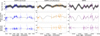 |
Fig. 11 The RV time series used in the GJ 1132 RV modeling. The top row shows the mean-subtracted RV-time series for each instrument, with the maximum a-posteriori RV model shown in black, while the middle row shows just the stellar activity component of the RV time series, with the corresponding best-fit stellar activity signal shown in black. The residuals between the best-fit model and each time series are shown in the bottom row. |
GJ 1252 RV analysis priors and parameters
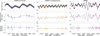 |
Fig. B.2 The RV time series used in the GJ 1252 RV modeling. The top row shows the mean-subtracted RV-time series for each instrument, with the maximum a-posteriori RV model shown in black, while the middle row shows just the stellar activity component of the RV time series, with the corresponding best-fit stellar activity signal shown in black. The residuals between the best-fit model and each time series are shown in the bottom row. |
LTT 3780 RV analysis priors and parameters
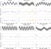 |
Fig. B.3 The RV time series used in the LTT 3780 RV modeling. Each set of three rows shows the RV time series for a given instrument. The top row shows the mean-subtracted RV-time series for each instrument, with the maximum a-posteriori RV model shown in black, while the middle row shows just the stellar activity component of the RV time series, with the corresponding best-fit stellar activity signal shown in black. The residuals between the best-fit model and each time series are shown in the bottom row. |
Appendix C Stellar abundances
Reported stellar abundances
All Tables
All Figures
|
Fig. 1 Model fit to the 1142.2 nm refractory Fe I line for star HD 260655. The colored lines represent different synthetic spectra, and the fainter gray lines represent the interpolated grid of spectra that was fit to the data, shown as a black dashed line. The best-fit abundance of [Fe/H] = −0.54 is shown as a darker gray line. It tracks the data over the line region very closely, and is delineated on either side by dashed gray lines. |
| In the text | |
|
Fig. 2 Detrended and phase-folded RV time series of GJ 1132 b (top) and GJ 1132 c (bottom). Different draws of the Keplerian models from our posterior are superimposed in black. The different colored markers correspond to different RV time series. The binned data points are shown as red squares. |
| In the text | |
|
Fig. 3 Phase-folded and detrended RV time series of GJ 1252 b (top) and GJ 1252 (c) (bottom). The best-fit Keplerian model is superimposed in black. The different colors and markers correspond to different RV time series. Binned data points are shown as red squares. |
| In the text | |
|
Fig. 4 Phase-folded and detrended RV time series of LTT 3780 b (top) and LTT 3780 c (bottom). The best-fit Keplerian model is superimposed in black. The different colors and markers correspond to different RV time series. Binned data points are shown as red squares. |
| In the text | |
|
Fig. 5 Generalized Lomb–Scargle periodogram of the archival HARPS RVs of GJ 1252. Each panel shows a different step of the one-planet model: the raw RVs (top); the RVs with the maximum a-posteriori (MAP) GJ 1252 b Keplerian model subtracted out (second); the RVs with the MAP stellar activity model subtracted out (third), and the RVs with both the MAP stellar activity model and GJ 1252 b Keplerian model subtracted out (bottom). Red lines corresponding to false alarm probabilities (FAPs) of 1% and 0.1% are overplotted, as are gray lines corresponding to 0.52 d (GJ 1252b period), 17.5d (GJ 1252 (c) period reported in Luque & Pallé 2022), and 64 d (the stellar rotation period reported in Shporer et al. 2020). |
| In the text | |
|
Fig. 6 Reanalyzed radii vs. masses of all the planets in our sample. The colors of data points are determined based on equilibrium temperature, according to the colorbar. Several composition curves are overlaid. A curve corresponding to an Earth-like composition from Zeng et al. (2019) is shown as solid green line. Curves corresponding to water mass fractions of 3% (dash-dotted) and 10% (dotted) are shown at 400, 700, and 1000 K, and are linearly interpolated based on the same pretabulated models discussed in Section 6.4. |
| In the text | |
|
Fig. 7 Set of posterior PDFs showing the distributions of CMFplanet, the CMF of the planets as measured from their masses and radii (orange), and CMFstar, the equivalent CMF as inferred from the refractory abundances of their host stars (blue), for each planet. Due to the high uncertainty in abundances for some stars, such as GJ 1252, some draws from the posterior are fit with very low [Fe/H] values and very high [Mg/H] and [Si/H] values, resulting in a very low CMFstar, causing a large amount of posterior draws to converge to CMFstar ≈ 0. |
| In the text | |
|
Fig. 8 Distribution of ΔCMF draws, as described in Section 6.1. A vertical black line corresponding to ΔCMF = 0 is overplotted. |
| In the text | |
|
Fig. 9 Correlation between CMFplanet and CMFstar for the nine hot super-Earths in our sample. The 95% upper limits are denoted with downward arrows. The line CMFplanet = CMFstar is overplotted as a dash-dotted black line. Our OLS fit with 1σ confidence intervals is shown in orange. The ODR fit is not shown here due to its high uncertainty. |
| In the text | |
|
Fig. 10 Distributions of the mean CMFplanet and CMFstar values as a function of the number of planets, for our current sample (top), for an observation campaign focused on improving the masses of planets already in our current sample (middle), and for an observation campaign focused on increasing the size of our sample (bottom). The dashed lines represent the median values of our CMF distributions, while the shaded regions represent the 1σ upper and lower regions. |
| In the text | |
|
Fig. 11 The RV time series used in the GJ 1132 RV modeling. The top row shows the mean-subtracted RV-time series for each instrument, with the maximum a-posteriori RV model shown in black, while the middle row shows just the stellar activity component of the RV time series, with the corresponding best-fit stellar activity signal shown in black. The residuals between the best-fit model and each time series are shown in the bottom row. |
| In the text | |
|
Fig. B.2 The RV time series used in the GJ 1252 RV modeling. The top row shows the mean-subtracted RV-time series for each instrument, with the maximum a-posteriori RV model shown in black, while the middle row shows just the stellar activity component of the RV time series, with the corresponding best-fit stellar activity signal shown in black. The residuals between the best-fit model and each time series are shown in the bottom row. |
| In the text | |
|
Fig. B.3 The RV time series used in the LTT 3780 RV modeling. Each set of three rows shows the RV time series for a given instrument. The top row shows the mean-subtracted RV-time series for each instrument, with the maximum a-posteriori RV model shown in black, while the middle row shows just the stellar activity component of the RV time series, with the corresponding best-fit stellar activity signal shown in black. The residuals between the best-fit model and each time series are shown in the bottom row. |
| In the text | |
Current usage metrics show cumulative count of Article Views (full-text article views including HTML views, PDF and ePub downloads, according to the available data) and Abstracts Views on Vision4Press platform.
Data correspond to usage on the plateform after 2015. The current usage metrics is available 48-96 hours after online publication and is updated daily on week days.
Initial download of the metrics may take a while.