| Issue |
A&A
Volume 710, June 2026
|
|
|---|---|---|
| Article Number | A30 | |
| Number of page(s) | 12 | |
| Section | Stellar atmospheres | |
| DOI | https://doi.org/10.1051/0004-6361/202659512 | |
| Published online | 28 May 2026 | |
Solar photospheric spectrum microvariability
III. Radial velocities and line profiles in magnetic active-region granulation
1
Lund Observatory, Division of Astrophysics, Department of Physics, Lund University,
22100
Lund,
Sweden
2
Zentrum für Astronomie der Universität Heidelberg, Landessternwarte,
Königstuhl 12,
69117
Heidelberg,
Germany
3
Leibniz-Institut für Astrophysik Potsdam,
An der Sternwarte 16,
14482
Potsdam,
Germany
4
Instituto de Astrofísica de Canarias, C/ Vía Láctea s/n,
38205
La Laguna, Tenerife,
Spain
5
Texas Advanced Computing Center, The University of Texas at Austin,
Austin,
TX
78758,
USA
★ Corresponding authors: This email address is being protected from spambots. You need JavaScript enabled to view it.
; This email address is being protected from spambots. You need JavaScript enabled to view it.
; This email address is being protected from spambots. You need JavaScript enabled to view it.
Received:
19
February
2026
Accepted:
7
April
2026
Abstract
Context. Finding low-mass planets around solar-type stars requires understanding the physical variability of the host star, which greatly exceeds the planet-induced radial-velocity modulation. Different solar photospheric absorption lines have slightly disparate responses to stellar activity, which should permit us to disentangle the wavelength shifts induced by exoplanets from those originating in stellar atmospheres.
Aims. Changing area coverages of magnetic active-region granulation (faculae and plage) cause radial-velocity fluctuations of the disk-integrated solar spectrum, whose precise modeling requires active-region spectral line profiles. Hydrodynamic 3D modeling of granulation in magnetic fields extends previous nonmagnetic studies, revealing different line profiles and altered convective velocity shifts.
Methods. Different types of lines in the visual and near-infrared are examined in synthetic hyper-high-resolution spectra (λ/Δλ ~900 000), comparing nonmagnetic areas with those with strongly magnetic (240 mT = 2400 G) granulation. Results. Magnetic fields inhibit convective motions, decrease the energy flow, produce more symmetric lines, and remove the common blueshift with its familiar C-shaped bisectors. Unexpectedly, magnetic granulation displays convective redshifts. Their origin is traced to contributions from small areas, where hot and bright down-moving elements are created through shocks and adiabatic compression when rising gas is forced over into magnetically channeled downflows.
Conclusions. Understanding line formation in also stellar active regions is needed to simulate full-disk spectra toward exoEarth detections. Detailed shapes of spectral lines carry significant information, suggesting that hyper-high spectral resolution may ultimately be required.
Key words: instrumentation: spectrographs / methods: observational / techniques: radial velocities / Sun: granulation Sun: photosphere / stars: solar-type
© The Authors 2026
 Open Access article, published by EDP Sciences, under the terms of the Creative Commons Attribution License (https://creativecommons.org/licenses/by/4.0), which permits unrestricted use, distribution, and reproduction in any medium, provided the original work is properly cited.
This article is published in open access under the Subscribe to Open model. This email address is being protected from spambots. You need JavaScript enabled to view it. to support open access publication.
1 Introduction
Efforts are underway toward enabling the detection of exoEarths, i.e., planets of about one Earth mass, in approximately one-year orbits around solar-type stars. The most promising method appears to be the radial-velocity method, although the signal is minuscule: for an Earth-mass planet orbiting a solar-mass star in a one-year orbit, at most only 10 cm s−1 (e.g., Hall et al. 2018). Although hardware and software developments now approach such precision (e.g., Artigau et al. 2022; Blackman et al. 2020; Crass et al. 2021; Cretignier et al. 2021; Fischer et al. 2016; Ford et al. 2024; Gupta & Bedell 2024; O’Sullivan & Aigrain 2024; Rackham et al. 2023; Salzer et al. 2025; Wilken et al. 2012; Zhao et al. 2026), such an exoplanet signal is overshadowed by much greater intrinsic stellar variability. To reach adequate sensitivity thus requires an understanding of the complexities of stellar atmospheric dynamics and spectral line modulation. A step toward exoEarth detection can be to identify dissimilar spectral lines (e.g., strong or weak, neutral or ionized, high or low excitation, atomic or molecular, short or long wavelengths, magnetically sensitive or not), with disparate responses to stellar activity, in order to disentangle wavelength shifts induced by exoplanets from those originating in solar-type atmospheres.
On the theoretical side, simulations with time-dependent 3D magnetohydrodynamics (MHD) now provide quite realistic descriptions of solar photospheric spectral-line-forming regions. Using the output from such simulations as arrays of time-dependent 3D atmospheres, complete stellar spectra can be computed, incorporating full transition databases such as VALD1 (Heiter et al. 2015; Ryabchikova et al. 2015), while sampling wavelengths with a hyper-high spectral resolution, λ/Δλ ~ 1 000 0002 (Chiavassa et al. 2018; Dravins et al. 2021a,b; Dravins & Ludwig 2023).
Nonmagnetic granulation covers most of the solar surface and provides most of the solar irradiance. In Paper I (Dravins & Ludwig 2023), sequences of synthetic spectra computed from corresponding 3D simulations were examined to identify patterns of short-term variability in the quiet Sun. The second-largest contribution to solar irradiance comes from plage and faculae areas of magnetic granulation. Magnetic fields disturb and dampen the convective velocity patterns, cause different asymmetries of the line profiles, and modify wavelength shifts. The varying area coverage of magnetic granulation during the solar cycle appears to be the main driver for longer-term changes in solar apparent radial velocity (Lakeland et al. 2024; Meunier et al. 2010a,b, 2024). While contributions from sunspots also affect spectral line shapes (Komori et al. 2025), their fraction of the solar photospheric flux is modest.
2 Appearance of magnetic granulation on the Sun
Much of the small-scale magnetic fields across granulation outside sunspots is outlined by the bright network. This magnetic network appears bright in various spectral regions, in particular in molecular and other temperature-sensitive lines. Among these, observations and modeling in the G-band are particularly extensive (e.g., Berger et al. 2004; Kuridze et al. 2025; Rouppe van der Voort et al. 2005). Similarly to other stronger lines, the network is also visible in the wings of Na I D1 (Jess et al. 2010; Keys et al. 2013, 2026). At high spatial resolution, it resolves into solar filigrees (sometimes called bright points, although not really point-like), occupying the spaces between granules. The corresponding appearance in the chromosphere is more smeared out, apparently reflecting the expansion of magnetic flux into higher layers.
A review of magnetic fields in the quiet Sun is given by Bellot Rubio & Orozco Suárez (2019). Different spectral lines have varying sensitivities to the magnetic field strength (Sinjan et al. 2024; Quintero Noda et al. 2021), while near-infrared lines might be especially valuable for mapping fields in the deeper photospheric layers (Hahlin et al. 2023; Lagg et al. 2016). Values on the order of 160 mT (1600 G) seem characteristic for actual intergranular field strengths (Bellot Rubio & Orozco Suárez 2019; de Wijn et al. 2009; Salhab et al. 2018; Stein 2012), while fields in sunspots may extend to 400 mT and beyond.
Convective blueshifts are suppressed in magnetically disturbed granulation and line profile asymmetries, and wavelength shifts are observed to gradually change when approaching and entering plage regions of progressively higher magnetic activity, as delineated by increasingly bright flux in the Ca II K line or by greater filling factors for the magnetic flux (e.g., Brandt & Solanki 1990; Cavallini et al. 1985, 1986, 1988, 1989). For strong lines formed high in the atmosphere, even inverted line asymmetries are observed, although their origins probably lie in more complex chromospheric dynamics (e.g., Uitenbroek 2006).
3 CO5BOLD models of the solar photosphere
In Paper I (Dravins & Ludwig 2023) and earlier, spectra from 3D simulations of the quiet nonmagnetic solar granulation were examined. We now turn to magnetic variants. A sequence of MHD CO5BOLD solar models were computed with the same resolution as in the nonmagnetic case by modeling a Cartesian box-in-a-star of 140 × 140 × 150 grid cells, with horizontal step sizes Δx = Δy = 40 km and vertical Δz = 15 km (for details of these computations, see Freytag et al. 2012 and Tremblay et al. 2013).
These magnetic simulations represent a range of average flux densities ⟨Bz⟩ from zero to 320 mT = 3200 G (Ludwig et al. 2023). The total net magnetic flux was set by initial conditions and preserved during the modeling sequence, with boundary conditions forcing field lines to pass orthogonally through the top and bottom boundaries of the simulation volumes. Thus, the horizontally averaged magnetic flux density remains constant during the evolution of the magnetized flow. To generate the initial model, a unipolar and homogeneous vertical magnetic field was added to a nonmagnetic temporal snapshot. After injecting such a magnetic flux in 3D atmospheric structures, its development can be followed with magnetic flux concentrating around intergranular lanes, the magnetic forces being balanced by gas pressure and dynamic effects, resulting in a somewhat disturbed and disrupted granulation structure. Radiative transfer is treated in 12 opacity bins and the simulations are advanced by a Harten-Lax-van Leer (HLL) solver, stabilized with additional turbulent viscosity and entropy diffusion. Irrespective of the magnetic flux, the heat content of the inflowing material was kept constant. By limiting the maximum Alfvén speed, all simulations could be run with a uniform time step of Δt = 0.2 s, even for the highest magnetic field strengths. Each simulation covers 12.5 hours of solar time, including initial relaxation. This time is substantially longer than for the nonmagnetic models, thus permitting us to follow the slower evolution of magnetic features. The vertical extent of the simulation box is 2250 km, and its top layer corresponds to Rosseland optical depth log τ = −6.5 in the nonmagnetic case and log τ = −6.6 for the 240 mT magnetic model (for details, including synthetic surface images for different magnetic flux levels and at different limb angles, see Ludwig et al. 2023).
Somewhat similar surface magnetoconvection has been modeled by Beeck et al. (2015a), Bhatia et al. (2022, 2026), Khomenko et al. (2018), Norris et al. (2023), Salhab et al. (2018), Shukla et al. (2026), Vögler et al. (2005), with spectral features computed by Beeck et al. (2015b); Smitha et al. (2021), and others. The radiative properties of these MHD simulations appear to be qualitatively consistent and indicate that, as long as the magnetic field is sufficiently weak, the radiative flux is enhanced by the presence of magnetic flux concentrations, but reverses somewhere around ⟨Bz⟩ = 50 mT. Gradually, darker features become increasingly prominent in the simulations with larger magnetic fluxes. For our strongest fields, ⟨Bz⟩ = 320 mT, the structures start to resemble sunspot umbrae; the magnetic flux density can locally reach very high values, with convection now restricted to narrow, almost field-free plumes of high upward velocities. In the synthetic continuum intensity images, these plumes resemble bright and moving umbral dots, often with the visual appearance of coffee beans (see Ludwig et al. 2023 and Fig. 9).
A significant reduction of the bolometric radiative flux follows in these stronger fields, and with even stronger flux concentrations the surface convection is inhibited and spots start to develop. With appropriate boundary conditions, models of umbrae and penumbrae structures can then be constructed (Panja et al. 2020; Schüssler & Vögler 2006; Smitha et al. 2025). The more moderate field strengths treated here reduce the overall heat flux, lower the average surface temperature, and cause many spectral lines to strengthen, similarly to stars somewhat cooler than the Sun (Fig. 1), even if they may weaken inside specific magnetic features. However, the present simulations are not to model specific magnetic elements, but rather to estimate how radial velocities and line profiles are affected when an extended area of granulation is modified by the presence of magnetic flux.
3.1 Limitations of magnetic models
Nonmagnetic granulation can be modeled from basic principles, using the fundamental parameters of stellar temperature, surface gravity, and chemical composition. Different models may apply different physical, mathematical, or numerical approximations, and the ensuing spectral synthesis may be carried on different levels of sophistication, but there are no further freely adjustable physical parameters. However, magnetic granulation introduces additional degrees of freedom, especially when modeling an entire star. Not only can the area coverage and latitudinal and longitudinal surface distributions be different, but also the distribution of strengths within the magnetic flux concentrations. For the spectral synthesis, an additional complication (or opportunity) comes with the possible treatment of magnetically sensitive lines. Thus, results from magnetic granulation cannot be expected to be singularly unique, but may have to be evaluated for a series of different magnetic field strengths and geometries; alternatively, one can look for characteristic line-profile signatures that differ between magnetic and nonmagnetic regions. Nonmagnetic simulations have in the past been verified against solar surface images, movies, and spectra, enabling successive fine-tuning of such models, but corresponding tests for magnetically well-defined samples are scarce (also because their atmospheric structures may be at or below observational resolution limits) and their models may still have room for improvement.
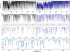 |
Fig. 1 Examples of synthetic spectra at the solar disk center, μ = 1, for the nonmagnetic (left) and the magnetic 240 mT (2400 G) simulation, expanded in wavelength from top down. Each section is normalized locally while the lower frame shows line identifications. From that region, the lines of Fe II 449.1405 and Fe II 450.8288 nm were selected for detailed study (Fig. 4 below). The wavelength scale denotes values in air. |
3.2 Synthetic spectra from MHD simulations
For these initial examinations of synthetic line profiles, a strong-field MHD model with 240 mT = 2400 G was selected (referred to below as magnetic granulation). This field strength can be seen to represent the strongest-field granulation in active plage or facular areas or perhaps umbral dots, with a flux density between the field-free situation and a fully developed sunspot umbra.
From the CO5BOLD simulation volumes, spatially and temporally averaged line profiles were computed in local thermodynamic equilibrium (LTE) using the ASS ϵ ET code (Koesterke et al. 2008). Calculations were made for the full spectral range of 120–3000 nm, and for 20 largely uncorrelated snapshots in time during the simulation. The spectra incorporate practically all relevant atomic and molecular transitions with a wavelength sampling corresponding to the hyper-high resolving power of λ/Δλ ~900 000. For different elevation and azimuth angles, the spectra were computed on a grid of 47 × 47 points (each of horizontal extent 120 × 120 km2, subsampled from 3 × 3 pixels in the hydrodynamic simulation). Integrated sunlight is computed by appropriately interpolating and summing spectra from different μ-values, somewhat analogous to how full-disk signatures were synthesized by Cegla et al. (2019), Frame et al. (2025), or Palumbo et al. (2022). The magnetic structures alter the shapes of spectral lines (Holzreuter & Solanki 2012, 2015; Holzreuter et al. 2025), while pairs of lines with disparate Landé geff factors, and thus different magnetic sensitivities, should be able to more directly diagnose field properties (Solanki 1993; Smitha & Solanki 2017). However, in the current calculations, Zeeman broadening or splitting is not included, and neither are solar rotational broadening or gravitational redshift (Figs. 1 and 2). For later studies, especially concerning specific magnetic structures, this should permit the indirect magnetic effect on the spectral lines to be separated, as studied here (via the altered flow field) from the direct magnetic effect (via Zeeman broadening).
Precision radial velocities are measured as a statistical average over many thousands of photospheric lines, where the different behavior between individual single lines normally is not measurable. Larger line groups may realistically be segregated against simple parameters such as line depth or wavelength region, and lines representing such subgroups were selected for the present study. However, given that the many lines entering radial-velocity measurements have varied dependences on Zeeman signatures and non-LTE sensitivities, the selected ones should be seen as generic representatives for their particular groups of line strength and wavelength region. In particular, by being largely unblended, they should more clearly show how line shapes are molded and shaped by the altered gas flow patterns and temperature structures in magnetically modified granulation.
The accuracy of synthetic spectra is ultimately limited by the quality of atomic and molecular data. Current spectra include data from more than half a million atomic lines, compiled from a multitude of sources, sometimes with variable accuracy. The input wavelengths for the spectral synthesis are specified in nanometers to four decimal places. At λ500 nm, the final decimal corresponds to a velocity of 60 m s−1, which is one limiting parameter in comparing modeled lineshifts to observed ones. Even if the laboratory values were perfectly known, they are not specified to closer than these four decimal places and, in any case, they typically have errors of comparable magnitude, contributing further noise between synthetic and observed velocity shifts. However, differential shifts within synthetic spectra, are not affected by such errors, except for higher-order effects due to possibly imprecise wavelength superpositions of blending lines. The absolute wavelength shifts discussed below refer to the nominal laboratory values.
Line shape and wavelength variations between differently magnetic regions have been studied in the past. However, such observations have been of relative wavelength shifts or between different positions in the line bisectors. Even with a very accurate spectrometer calibration, any deduction of absolute wavelength shifts depends on the accuracy of the laboratory wavelengths. One main difference to the present work is that, by using numerically exact values for the transition wavelengths in the synthetic spectra, absolute lineshifts can be deduced relative to those values, even if they do not precisely agree with the true (but not perfectly known) laboratory values.
A general limitation of photospheric modeling is that its vertical extent does not fully embrace the formation heights of stronger lines. In addition, boundary conditions might cause spurious temperature fluctuations near the upper boundary, contributing to emission artifacts in the cores of the strongest lines. Thus, lines formed in the uppermost photosphere or lower chromosphere cannot be expected to be precisely reproduced. Nevertheless, we still examined the behavior of some strong lines such as the Mg I triplet, the Na I D lines, and the infrared Ca II triplet: even if their cores cannot be faithfully modeled, their largely photospheric flanks and wings should still be approximately reproduced and might confirm trends seen in other lines when going toward higher atmospheric layers.
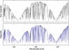 |
Fig. 2 Synthetic spectra in the Ca II H & K line region: nonmagnetic (top) and 240 mT (2400 G) magnetic models. (However, the bottoms of these very strong lines are not precisely reproduced by the present modeling.) From this particular region, Fe I 393.2627 and Fe I 396.7421 nm lines, superposed onto the extended and sloping absorption wings of the K and H lines, were selected for examination (Fig. 7 below). These spectra are for the integrated solar disk. |
4 Selecting and fitting representative spectral lines
The spectral region selected was 350–1000 nm, spanning the observational regions for current visual and near-infrared radial-velocity instruments (e.g., Bouchy et al. 2025; Doyon et al. 2025; Lo Curto et al. 2024; Mayor et al. 2003). About 50 lines of various strengths in different wavelength regions that appeared largely unblended in both the nonmagnetic and magnetic spectra were selected for closer examination. Given that Fe lines are ubiquitous throughout the spectrum and are commonly used for various atmospheric diagnostics and velocity shifts, most lines are Fe I and Fe II, many the same as in Paper I (Table A.1). To also include a very broad photospheric line, a Ca I was chosen (even though no longer fully unblended), and lines of varying strength from several other species were also included.
All lines are asymmetric and variable during the simulation sequences. To practically examine dependences among various line parameters, the information in the line profiles needs to be parameterized. Following various tests of line-fitting parameters, a suitable approximation was found (as in Paper I) by fitting the synthetic line profiles with five-parameter Gaussian-like functions of the type y0 − a · exp[−0.5 · (|x − x0|/W)c], yielding y0 for the continuum level, a for the absorption depth, W as a measure of the line width, c for the degree of the line’s boxiness or pointedness, and x0 for the average wavelength. As illustrated in Fig. 3, this fitting provides one unique value for the radial velocity that refers to an average displacement of the line as a whole. The exact value that a radial-velocity spectrometer will obtain depends on the precise algorithm and type of weighting applied; however, the physical differences between different spectral lines are much greater than the plausible differences in the definition of such a spectral-line wavelength.
Very strong lines from the Mg I triplet, Na I D lines, and the infrared Ca II triplet were treated somewhat differently; the radial velocities were computed separately for their line cores and flanks. In the magnetic spectra, some of their cores start to exhibit irregular emission, which does not provide meaningful radial velocities, while the more photospheric line flanks still might.
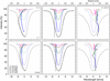 |
Fig. 3 Modeled and fitted line profiles. Left: profiles and bisectors for differently deep absorption lines, as obtained from time-averaged 3D simulations of nonmagnetic granulation. Wavelengths are in velocity units relative to each line’s laboratory wavelength. At the top, the bisector scale is expanded tenfold. The central column shows the same profiles from these simulations (dotted), now together with their fitted profiles (solid) using a five-parameter Gaussiantype function. Since the fitted profiles are symmetric, their dashed bisectors are vertical limes, defining each line’s average radial velocity. The right column shows the same lines in the 240 mT (2400 G) magnetic simulation. The upper row gives data for solar disk center, μ = 1; the lower row is for integrated sunlight. The lines are listed at the bottom left, in order of increasing line depth. Bisector wiggles for the strongest magnetic line are caused by blends in its broad wings. The effects of solar rotation and gravitational redshift are not included. |
5 Profiles and velocity shifts for different lines
A general property of photospheric lines from quiet nonmagnetic granulation is their asymmetry and convective blueshift, well studied both observationally and theoretically (e.g., Bergemann & Hoppe 2026; Reiners et al. 2016; Sheminova 2022). A characteristic signature is the marching progression of C-shaped bisectors for differently strong lines, with the weakest lines normally showing the largest blueshifts. In Fig. 3, such a sequence of lines with gradually increasing strengths is assembled, showing this familiar bisector pattern, with amplitudes at disk center being somewhat greater than in integrated sunlight from the full disk.
5.1 Lines of different strength
The central frames of Fig. 3 illustrate how this fitting procedure provides unique values for the average radial velocities of each line. The synthetic profiles (dotted) are fitted with the fiveparameter function, which is seen to very closely follow the synthetic profiles, the only exception being slight differences in the core and wings of the very broad Ca I line. Since the fitted profiles are symmetric, their bisectors are vertical lines, whose positions now define each line’s average radial velocity, as used in the later plots and tables. All wavelength scales are relative to the database values for laboratory wavelengths used as input to the spectral synthesis, and modeled lineshifts are thus not affected by possible errors in the laboratory values. However, even if these lines are selected to be apparently unblended, some astrophysical noise is contributed from numerous weak blending lines: the input catalog has on the order of 1000 lines per each nanometer interval and every line will also have at least slight contributions from the others.
The right panels of Fig. 3 show the same spectral lines from the magnetic simulation. In this case, their sequence of relative line strengths does not change much, although their bisectors do. The lines largely lose their asymmetries with their bisectors tending to become straight vertical lines (disregarding the bisector wiggles for the strongest magnetic line, which are caused by blends appearing in its broad line wings). Strikingly, the convective blueshift in nonmagnetic granulation is now instead replaced by a redshift. Analogous to the nonmagnetic case, this shift away from zero is more pronounced at disk center (top) than in integrated sunlight.
5.2 Closely related lines
Figure 4 examines these effects for three intermediate and strong lines selected to be very similar, except for their depths: Fe II λ 450.8288 nm, χ = 2.86 eV; Fe II λ 466.6758, χ = 2.83; Fe II λ 467.0182 nm, χ = 2.58 eV. Analogous to the nonmagnetic case, the largest shifts for the magnetic profiles are seen in the weaker lines, while the bottoms of the strongest lines show only modest displacements.
In addition to the synthetic data, observed spectra are shown (left) from the Jungfraujoch disk-center atlas (top; Delbouille et al. 1989) and from the integrated flux atlases of Kitt Peak (Kurucz et al. 1984) and Göttingen (Reiners et al. 2016), illustrating both similarities and typical differences. Wavelength shifts from the observational atlases refer to the same database values (to four decimal points in nanometers) as the synthetic lines, and are subject to roundoff errors of the true wavelength to this fourth decimal place, imprecisions in laboratory wavelengths, possible inaccuracies in the atlas wavelength scales, a somewhat different pattern of weak blending lines (whose wavelengths or strengths may not perfectly coincide with those in synthetic spectra); they can be affected by a slight line smearing by an extended spectrometer slit at solar disk center, full-disk line broadening due to solar rotation, and the solar gravitational redshift of 635 m s−1. The exact gravitational redshift value depends on the precise height of line formation (Cegla et al. 2012; Lindegren & Dravins 2003)3.
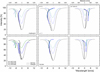 |
Fig. 4 Line profiles and bisectors for differently strong Fe II lines. The leftmost column shows observed data from the Jungfraujoch solar disk-center atlas (top) and the integrated solar flux atlases of Kitt Peak and Göttingen (bottom). Profiles from the nonmagnetic (center) and magnetic 240 mT = 2400 G simulations (right) are shown for disk center μ = 1 (upper row) and for integrated sunlight of a nonrotating Sun (lower row). The wavelength scales are relative to the laboratory values used as input to the simulations, while the observational atlases are affected by solar gravitational redshift of 635 m s−1 and likely errors in laboratory wavelengths. |
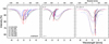 |
Fig. 5 Weak lines at solar disk center, μ = 1. Shown are the line profiles and bisectors from the Jungfraujoch atlas (left). Numerous lines of comparable strength show similar behavior in both the nonmagnetic case (center) and in the 240 mT = 2400 G magnetic simulation (right). Wavelengths in observational atlases are affected by the solar gravitational redshift of 635 m s−1 and possible errors in laboratory wavelengths. |
5.3 Very weak lines
Figure 5, with seven lines from the disk center, illustrates the degree of similarities between the different weak lines. On the left are the observed profiles from the Jungfraujoch atlas, and the profiles and bisectors for the nonmagnetic and magnetic models. The lines of different species, and in different regions of the spectrum, display quite similar behavior. The observed Co I line is broader than the others, most probably due to its hyper-fine structure, an effect not treated in the synthetic spectra. Data for the full disk (not shown) are qualitatively similar.
5.4 Very strong lines
Figure 6 shows samples of the strongest lines at solar disk center; again, the full-disk data are not very different. The left column displays Mg I b2 and Na I D2 profiles in the Jungfraujoch atlas, the center and right their modeled nonmagnetic and magnetic line-core profiles; the very similar Mg I b1 and Na I D1 lines are also plotted. Due to the presence of blends across these broad lines, bisectors are fitted only to their deep cores; note the change of intensity scales.
The limited applicability of photospheric granulation models to the detailed formation of very strong lines in the upper photosphere (with contributions from the low chromosphere) is noted above. For these types of lines, additional issues arise because of likely non-LTE effects. The green magnesium triplet of Mg I b1 λ 518.3, b2 λ 517.2, and b3 λ 516.7 nm has coupled atomic energy levels such that these are transitions between one shared upper level and three different lower levels, thus contributing to the complexity of their formation (for a discussion of their formation and references, see Paper II, Dravins & Ludwig 2024).
Other strong lines behave similarly to the green Mg triplet. The two strong Na I D1 and D2 lines are used as diagnostics for the upper photosphere and the lower chromosphere (usually the weaker and less blended Na I D1). The infrared C II triplet lines at λ 849.8, λ 854.2, and λ 866.2 nm reflect activity in stars, and their behavior in the current modeling largely follows Mg I b and Na I D. However, in the magnetic model, spurious emission develops in the cores of these lines, limiting sensible radial-velocity determinations to the line flanks alone (Table A.1). Further details for these stronger lines are discussed in Paper II, in connection with observations of their longer-term variations in the spectrum of the Sun seen-as-a-star, compared to the classic chromospheric indicators of Ca II H & K.
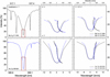 |
Fig. 6 Very strong lines at solar disk center. Left: Mg I b2 and Na I D2 lines in the Jungfraujoch atlas. Center: synthetic profiles and bisectors for their line cores (corresponding to the boxes at left), and also the related Mg I b1 and Na I D1 lines for the nonmagnetic simulation. Right: 240 mT = 2400 G magnetic case. The effects of solar rotation and gravitational redshift are not included. |
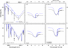 |
Fig. 7 Lines in special positions display special behavior. The weak Fe I 393.2627 and Fe I 396.7421 lines are superposed onto the extended absorption wings of the Ca II H & K lines and get their formation heights lifted through combining their opacities with those of the H&K line wings. The leftmost column shows their appearance in solar spectrum atlases (Kitt Peak full-disk, Jungfraujoch disk center). With vertical bisectors, the line cores are remarkably symmetric in both the nonmagnetic (center) and magnetic 240 mT = 2400 G case (right). |
6 Lines in particular positions
Some spectral lines combine with others, such as weak photospheric lines superposed onto the extended flanks of the very broad Ca II H&K lines. Although such lines would in isolation be ordinary ones, their formation now is affected by line-wing opacities or radiative transitions of the host line, leading them to sample different atmospheric conditions and – under the combined opacities with its host line – lifting its formation level into higher atmospheric layers. This behavior was discovered long ago for the hydrogen Balmer Hε line in the longward wing of Ca II H (Wilson 1938; Hinkle et al. 2000). Balmer lines are normally absorption features, but Hε appeared as a chromospheric-type emission in the spectrum of the cool giant star Arcturus, since seen in numerous other stars. On the Sun, high-resolution Hε spectroheliograms reveal a reversed granulation pattern, indicating enhanced formation heights (Krikova et al. 2023). Related solar phenomena include emission lines from rare earth elements and from Fe II, appearing in the Ca II H&K line wings, pointing to non-LTE effects.
The solar Hε is a broad and shallow absorption line, not suited for radial-velocity measurements. However, narrow absorption lines in similar positions in the Ca II H&K line wings can be expected to similarly sample the upper photosphere, with dampened or even inverted granulation contrast. Fig. 7 shows the behavior of two such weak Fe I absorption lines positioned in the flanks of, respectively, Ca II K and Ca II H. These were selected as being clean and apparently unblended (except for their host lines), with their appearances in spectral atlases for both disk center and full-disk spectra shown at left. Their behavior is different from ordinary lines in that the line cores are remarkably symmetric in both the nonmagnetic and magnetic versions, seen as vertical bisector sections (although the upper bisector slopes turn sharply toward the red due to the sloping Ca II pseudocontinua). The lack of any significant line-bottom asymmetry confirms that these lines are not formed in the deeper photosphere, but on levels where the granular velocity field has substantially lower amplitudes and/or less pronounced velocity-brightness correlations, and possibly also less variability.
7 Nonmagnetic and magnetic radial velocities
Figure 8 summarizes the velocity shifts for all ordinary lines (i.e., excluding the very strong ones and those in the Ca II H&K wings) as function of line depth and width. The velocities are as obtained from the five-parameter fits illustrated in Fig. 3. Convective velocities are dampened in the magnetic model, decreasing the velocity broadening and resulting in clearly narrower line profiles. Among the lines from the nonmagnetic model, their convective blueshifts tend to be greater for weaker lines, but there is no striking variation with line strength. Differences between weak and strong lines are more manifest in their different asymmetries and bisector shapes. Table A.1 gives detailed numbers, while its averages over different wavelength regions show some tendency for the shifts to decrease toward longer wavelengths, as expected from lower granulation contrast in the red. The sample is too small to isolate higher-order dependences on excitation potential, as can otherwise be identified for idealized and isolated synthetic lines (Dravins & Ludwig 2023). The unexpected and striking signature is the appearance of absolute redshifts in the magnetic spectra. Their amounts are smaller than the convective blueshifts in nonmagnetic granulation (full-disk spectra averages −308 vs. +130 m s−1) and, similarly, are most pronounced at disk center, becoming more smeared out in full-disk spectra.
In the nonmagnetic model, line widths in full-disk spectra are broader than at disk center, reflecting the contributions from developed horizontal velocities that enhance Doppler broadening toward the limb. The opposite is suggested in the magnetic model, apparently reflecting the smaller amplitudes in horizontal velocity fields.
8 Origin of redshifts in magnetic regions
The line profiles examined so far result from extensive averaging over the simulation sequence and do not directly reveal the specific origin of the redshifts. As studied in nonmagnetic granulation, spatially resolved line profiles display highly varying shapes, reflecting their formation in an inhomogeneous medium (e.g., Asplund 2005; Bergemann et al. 2019; Dravins & Nordlund 1990), while their averaged profiles and bisectors encode their statistical distributions. Tracing the origin of the magnetic redshifts requires a similarly detailed examination of the build-up of the averaged lines, where many thousands of spatially and temporally resolved profiles are combined.
One representative temporal snapshot was selected and corresponding solar surface maps in Fig. 9 illustrate the lineshift variation across the model surface and its relation to various surface features. In particular, contours of vertical velocity νz = 0 indicate locations where upflows turn into downflows. A large fraction of the area is dominated by slow motions, where the convective velocities have been dampened by the magnetic fields. Dynamically relevant features producing local redshifts are mostly associated with small areas of high intensity (bright points), so that averaged over space and time, the redshift injected from these localities causes a bias. The dark inner parts of these bright points are associated with upflows (e.g., the feature at x,y = [3.7, 0.3] Mm), leading to a local blueshift of the line. Remarkably, the highest continuum brightness often coincides with the νz = 0 contour, indicating that heating (by adiabatic compression, shocks, friction) is occurring when gas is forced to turn over from narrow upflows into magnetically channeled downflows. The width of these features is very small, less than 100 km, and is close to the resolution limit of these simulations, and requires higher-resolution models to reveal further details.
Spatially resolved profiles were calculated for 40 × 40 km2 pixels, shown in Fig. 10 for the weak Fe I 683.7006 nm and the strong line Fe I 524.7050 nm line. To limit cluttering, each plot shows only 1% of the profiles in one snapshot, spatially uniformly sampled across the simulation area. To examine how the magnetic redshift signature evolves, line syntheses were carried out for models with successively higher magnetic fields. In addition to the currently examined 240 mT simulation, Fig. 10 also shows profiles from a corresponding field-free simulation, and one with a weaker 120 mT field. The redshift signature develops gradually and the main mechanism is that magnetically channeled downflows become brighter in magnetoconvection, even brighter than upflows. Another effect that differs from the nonmagnetic case is that the surface area fractions of up- and downflows become more equal or that downflow areas even dominate. On some level of approximation, most of the surface can be seen as behaving rather neutrally, but the small bright points (despite subtending only a tiny fraction of the area) inject sufficiently many redshifted line components to bias the global average. The origin of magnetic redshifts is thus qualitatively different from nonmagnetic blueshifts, where the upflows are large, bright, and blueshifted, but the downflows are small, dark, and redshifted, which results in a net blueshift of a line, with its familiar C-shaped bisector.
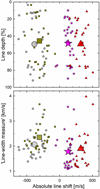 |
Fig. 8 Radial-velocity shifts for ordinary lines (Table A.1). The gray circles are lines from the nonmagnetic simulation at solar disk center; the dark squares are for the full solar disk. The red triangles are from the magnetic model at disk center; the purple stars are magnetic full disk. Small symbols denote specific spectral lines, large symbols their total average. Line depth denotes absorption in units of the local continuum; weak lines thus carry small numbers. Each line’s average wavelength and line width measure is obtained from fitting the synthetic profiles to a symmetric five-parameter Gaussian-type function. The modeled lines are not affected by either solar rotation or gravitational redshift. |
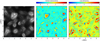 |
Fig. 9 Brightness, gas velocities, and radial velocities in one temporal snapshot of the magnetic 3D simulation for 240 mT = 2400 G. Left: continuum intensity at solar disk center (μ = 1) near Fe I 683.7 nm. Center: vertical gas velocity (measured positive rising upward in the atmosphere) over a horizontal plane near Rosseland optical depth unity. The thin black lines depict the vz = 0 contour separating the up- and downflows. Right: spectroscopic lineshifts for Fe I 683.7 nm (measured positive redshifted if receding downward into the atmosphere, thus inverting the color scale). |
9 Conclusions and outlook
In this paper, line profiles and wavelength shifts arising in strongly magnetic granulation were examined. Gradually varying solar surface area coverage by magnetic and nonmagnetic components permits to reproduce the general solar-cycle changes in its apparent radial velocity (Lakeland et al. 2024; Meunier et al. 2010a). With detailed line profile and lineshift information, such variability could be more precisely modeled even if data for a mixture of magnetic field strengths may be needed. Paper I theoretically examined short-term radial-velocity jittering in nonmagnetic granulation. Forthcoming work will explore such short-term variability in magnetic granulation, with the aim of identifying further measurable photospheric parameters that could eventually lead toward exoEarth detections.
Finding exoEarths will be challenging, but spectral-line wavelengths remain the most precisely measurable parameter, rather than line depth, width, or shape. Optimal detection algorithms will profit from including the additional information contained in the differential behavior of individual spectral lines, as already experienced in observational studies (Al Moulla et al. 2022, 2024; Anna John et al. 2025; Cretignier et al. 2020; Deming et al. 2024; Dumusque 2018; Meunier et al. 2017; Miklos et al. 2020; Thompson et al. 2020; Wise et al. 2022). To fully understand how to optimally mitigate stellar radial-velocity fluctuations toward exoEarth detection thus requires an understanding of the origins of specific line-profile variability and how their variations relate to wavelength displacements.
Although simulations of 3D atmospheres now begin to reach a certain maturity, quite different levels of sophistication are possible for the ensuing computation of synthetic spectra, eventually perhaps envisioning full non-LTE treatments with Zeeman-sensitive line components for those lines with a nonzero Landé geff-factor and a connection to the lower chromosphere, among other factors. The significance of non-LTE effects for seemingly ordinary photospheric lines is also suggested by studies of how different assumed levels of chromospherically influenced temperatures in the upper photosphere affect 1D non-LTE line formation in modeled G2 V stars (Vieytes et al. 2025). The response to different levels of chromospheric heating is found to be markedly different among various Fe I lines, even those with similar strengths and at nearby wavelengths, carrying a promise that they contain additional signatures of solar atmospheric modulation. Such lines could be selected to observationally search for their variability although challenging non-LTE 3D calculations might be needed for their fuller understanding (Bergemann & Hoppe 2026; Holzreuter et al. 2025; Lind & Amarsi 2024). Searches for planets around magnetically active stars face additional complications (e.g., Hébrard et al. 2014).
The new PoET telescope at ESO VLT on Paranal is a significant addition to Sun-as-as-star facilities (Santos et al. 2025). In addition to providing spectra of the Sun-as-a-star with the ESPRESSO spectrometer’s high resolving power approaching ~200 000, it will be able to select limited portions of the solar disk to examine local line shapes and shifts, potentially enabling novel tests of MHD model atmospheres. The large ANDES spectrometer is being built for the ESO ELT (Palle et al. 2025). While it will have outstanding light-collecting power, the challenges of interfacing a realistically large cross-dispersed échelle spectrometer to an extremely large telescope, limits its spectral resolution to ranges that are similar to those of current instruments. In the longer term, one could certainly also wish for hyper-high resolutions of λ/Δλ ~ 1 000 000, corresponding to those in the present theoretical work, but then possibly requiring diffraction-limited adaptive-optics photonic instruments to limit their physical size. The NIRPS radial-velocity spectrometer takes advantage of adaptive optics (Bouchy et al. 2025) to limit its size, but to realize the same at an extremely large telescope for the shorter visual wavelengths remains an interesting challenge.
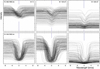 |
Fig. 10 Spatially resolved line profiles across the simulation area at solar disk center illustrate how the convective blueshift in the field-free case gradually changes into a magnetic redshift. From left to right, the weak Fe I 683.7006 nm and strong Fe I 524.7050 nm lines are shown (at the same pixels in the same snapshot) from simulations with fields = 0, 120, and 240 mT (0, 1200, 2400 G). The nonmagnetic convective blueshift is caused by large, bright, and blueshifted granules dominating over spatially narrow, dark, and redshifted downflows. In the magnetic case, the surface areas of up- and downflows are more equal, the velocities are lower, while the redshifted contributions from small bright elements bias the average. |
Acknowledgements
The work by D.D. is supported by grants from The Royal Physiographic Society of Lund. C.A.P. is thankful for funding from the Spanish government through grants AYA2014-56359-P, AYA2017-86389-P and PID2020-117493GB-100. Important contributions to the development of the CO5BOLD model family have been made by Bernd Freytag of Uppsala University. Parts of this paper were completed by D.D. during a stay as a Scientific Visitor at the European Southern Observatory in Santiago de Chile. Extensive use was made of NASA’s ADS Bibliographic Services and the arXiv® distribution service. We thank the anonymous referee for multiple insightful comments, which have improved the clarity of the text.
References
- Al Moulla, K., Dumusque, X., Cretignier, M., et al. 2022, A&A, 664, A34 [NASA ADS] [CrossRef] [EDP Sciences] [Google Scholar]
- Al Moulla, K., Dumusque, X., & Cretignier, M. 2024, A&A, 683, A106 [NASA ADS] [CrossRef] [EDP Sciences] [Google Scholar]
- Anna John, A., Al Moulla, K., O’Sullivan, N. K., et al. 2025, MNRAS, 543, 1974 [Google Scholar]
- Artigau, É., Cadieux, C., Cook, N. J., et al. 2022, AJ, 164, 84 [NASA ADS] [CrossRef] [Google Scholar]
- Asplund, M. 2005, ARA&A, 43, 481 [Google Scholar]
- Beeck, B., Schüssler, M., Cameron, R. H., et al. 2015a, A&A, 581, A42 [NASA ADS] [CrossRef] [EDP Sciences] [Google Scholar]
- Beeck, B., Schüssler, M., Cameron, R. H., et al. 2015b, A&A, 581, A43 [NASA ADS] [CrossRef] [EDP Sciences] [Google Scholar]
- Bellot Rubio, L., & Orozco Suárez, D. 2019, Liv. Rev. Solar Phys., 16, 1 [CrossRef] [Google Scholar]
- Bergemann, M., & Hoppe, R. 2026, Liv. Rev. Comp. Astroph., in press, [arXiv:2511.04254] [Google Scholar]
- Bergemann, M., Gallagher, A. J., Eitner, P., et al. 2019, A&A, 631, A80 [NASA ADS] [CrossRef] [EDP Sciences] [Google Scholar]
- Berger, T. E., Rouppe van der Voort, L. H. M., Löfdahl, M. G., et al. 2004, A&A, 428, 613 [NASA ADS] [CrossRef] [EDP Sciences] [Google Scholar]
- Bhatia, T. S., Cameron, R. H., Solanki, S. K., et al. 2022, A&A, 663, A166 [NASA ADS] [CrossRef] [EDP Sciences] [Google Scholar]
- Bhatia, T.S., Cameron, R. H., Solanki, S. K., et al. 2026, A&A, 706, A308 [NASA ADS] [CrossRef] [EDP Sciences] [Google Scholar]
- Blackman, R. T., Fischer, D. A., Jurgenson, C. A., et al. 2020, AJ, 159, 238 [CrossRef] [Google Scholar]
- Bouchy, F., Doyon, R., Pepe, F., et al. 2025, A&A, 700, A10 [NASA ADS] [CrossRef] [EDP Sciences] [Google Scholar]
- Brandt, P. N., & Solanki, S. K. 1990, A&A, 231, 221 [NASA ADS] [Google Scholar]
- Cavallini, F., Ceppatelli, G., & Righini, A. 1985, A&A, 143, 116 [NASA ADS] [Google Scholar]
- Cavallini, F., Ceppatelli, G., & Righini, A. 1986, A&A, 158, 275 [NASA ADS] [Google Scholar]
- Cavallini, F., Ceppatelli, G., & Righini, A. 1988, A&A, 205, 278 [NASA ADS] [Google Scholar]
- Cavallini, F., Ceppatelli, G., & Righini, A. 1989, Sol. Stellar Granulation, NATO ASI 263, 283 [Google Scholar]
- Cegla, H. M., Watson, C. A., Marsh, T. R., et al. 2012, MNRAS, 421, L54 [NASA ADS] [Google Scholar]
- Cegla, H. M., Watson, C. A., Shelyag, S., et al. 2019, ApJ, 879, 55 [NASA ADS] [CrossRef] [Google Scholar]
- Chiavassa, A., Casagrande, L., Collet, R., et al. 2018, A&A, 611, A11 [NASA ADS] [CrossRef] [EDP Sciences] [Google Scholar]
- Crass, J., Gaudi, B. S., Leifer, S., et al. 2021, Extreme Precision Radial Velocity Working Group Final Report [arXiv:2107.14291] [Google Scholar]
- Cretignier, M., Dumusque, X., Allart, R., et al. 2020, A&A, 633, A76 [NASA ADS] [CrossRef] [EDP Sciences] [Google Scholar]
- Cretignier, M., Dumusque, X., Hara, N. C., et al. 2021, A&A, 653, A43 [NASA ADS] [CrossRef] [EDP Sciences] [Google Scholar]
- Delbouille, L., Roland, G., & Neven, L. 1989, Atlas Photométrique du Spectre Solaire de λ 3000 a λ 10000 (Liège: Université de Liège, Institut d’Astrophysique) [‘Jungfraujoch atlas’] Digital version: http://bass2000.obspm.fr [Google Scholar]
- Deming, D., Llama, J., & Fu, G. 2024, AJ, 167, 34 [NASA ADS] [CrossRef] [Google Scholar]
- de Wijn, A. G., Stenflo, J. O., Solanki, S. K., et al. 2009, Space Sci. Rev., 144, 275 [NASA ADS] [CrossRef] [Google Scholar]
- Doyon, R., Bouchy, F., Pepe, F., et al. 2025, The Messenger, 194, 13 [Google Scholar]
- Dravins, D., & Ludwig, H.-G. 2023, A&A, 679, A3 (Paper I) [NASA ADS] [CrossRef] [EDP Sciences] [Google Scholar]
- Dravins, D., & Ludwig, H.-G. 2024, A&A, 687, A60 (Paper II) [NASA ADS] [CrossRef] [EDP Sciences] [Google Scholar]
- Dravins, D., & Nordlund, Å 1990, A&A, 228, 184 [NASA ADS] [Google Scholar]
- Dravins, D., Ludwig, H.-G., & Freytag, B. 2021a, A&A, 649, A16 [NASA ADS] [CrossRef] [EDP Sciences] [Google Scholar]
- Dravins, D., Ludwig, H.-G., & Freytag, B. 2021b, A&A, 649, A17 [NASA ADS] [CrossRef] [EDP Sciences] [Google Scholar]
- Dumusque, X. 2018, A&A, 620, A47 [NASA ADS] [CrossRef] [EDP Sciences] [Google Scholar]
- Fischer, D. A., Anglada-Escude, G., Arriagada, P., et al. 2016, PASP, 128, 066001 [Google Scholar]
- Ford, E. B., Bender, C. F., Blake, C. H., et al. 2024, arXiv e-prints [arXiv:2408.13318] [Google Scholar]
- Frame, G., Cegla, H. M., Witzke, V., et al. 2025, MNRAS, 539, 2248 [Google Scholar]
- Freytag, B., Steffen, M., Ludwig, H.-G., et al. 2012, J. Comp. Phys., 231, 919 [NASA ADS] [CrossRef] [Google Scholar]
- Gupta, A. F., & Bedell, M. 2024, AJ, 168, 29 [Google Scholar]
- Hahlin, A., Kochukhov, O., Rains, A. D., et al. 2023, A&A, 675, A91 [NASA ADS] [CrossRef] [EDP Sciences] [Google Scholar]
- Hall, R. D., Thompson, S. J., Handley, W., et al. 2018, MNRAS, 479, 2968 [NASA ADS] [CrossRef] [Google Scholar]
- Hébrard, É. M., Donati, J.-F., Delfosse, X., et al. 2014, MNRAS, 443, 2599 [Google Scholar]
- Heiter, U., Lind, K., Asplund, M., et al. 2015, Phys. Scr, 90, 054010 [CrossRef] [Google Scholar]
- Hinkle, K., Wallace, L., Valenti, J., Harmer, D. 2000, Visible and Near Infrared Atlas of the Arcturus Spectrum 3727–9300 Å, (San Francisco: Astron. Soc. Pacific) [Google Scholar]
- Holzreuter, R., & Solanki, S. K. 2012, A&A, 547, A4 [Google Scholar]
- Holzreuter, R., & Solanki, S. K. 2015, A&A, 582, A101 [NASA ADS] [CrossRef] [EDP Sciences] [Google Scholar]
- Holzreuter, R., Smitha, H. N., & Solanki, S. K. 2025, A&A, 697, A105 [NASA ADS] [CrossRef] [EDP Sciences] [Google Scholar]
- Immerschitt, S., & Schroeter, E. H. 1989, A&A, 208, 307 [Google Scholar]
- Ishikawa, R., Tsuneta, S., Kitakoshi, Y., et al. 2007, A&A, 472, 911 [NASA ADS] [CrossRef] [EDP Sciences] [Google Scholar]
- Jess, D. B., Mathioudakis, M., Christian, D. J., et al. 2010, ApJ, 719, L134 [NASA ADS] [CrossRef] [Google Scholar]
- Keys, P. H., Mathioudakis, M., Jess, D. B., et al. 2013, MNRAS, 428, 3220 [NASA ADS] [CrossRef] [Google Scholar]
- Keys, P. H., Campbell, R. J., Magill, D. K. J., et al. 2026, ApJ, 999, 201 [Google Scholar]
- Khomenko, E., Vitas, N., Collados, M., et al. 2018, A&A, 618, A87 [NASA ADS] [CrossRef] [EDP Sciences] [Google Scholar]
- Koesterke, L., Allende Prieto, C., & Lambert, D. L. 2008, ApJ, 680, 764 [NASA ADS] [CrossRef] [Google Scholar]
- Komori, C., Brewer, J. M., & Zhao, L. L. 2025, AJ, 170, 209 [Google Scholar]
- Kostik, R., & Khomenko, E. V. 2012, A&A, 545, A22 [NASA ADS] [CrossRef] [EDP Sciences] [Google Scholar]
- Krikova, K., Pereira, T. M. D., & Rouppe van der Voort, L. H. M. 2023, A&A, 677, A52 [NASA ADS] [CrossRef] [EDP Sciences] [Google Scholar]
- Kuridze, D., Wöger, F., Uitenbroek, H., et al. 2025, ApJ, 985, L23 [Google Scholar]
- Kurucz, R. L., Furenlid, I., Brault, J., Testerman, L. 1984, National Solar Observatory Atlas, Sunspot, New Mexico: National Solar Observatory [‘Kitt Peak atlas’] Digital version: http://diglib.nso.edu [Google Scholar]
- Lagg, A., Solanki, S. K., Doerr, H.-P., et al. 2016, A&A, 596, A6 [NASA ADS] [CrossRef] [EDP Sciences] [Google Scholar]
- Lakeland, B. S., Naylor, T., Haywood, R. D., et al. 2024, MNRAS, 527, 7681 [Google Scholar]
- Lind, K., & Amarsi, A. M. 2024, ARA&A, 62, 475 [Google Scholar]
- Lindegren, L., & Dravins, D. 2003, A&A, 401, 1185 [NASA ADS] [CrossRef] [EDP Sciences] [Google Scholar]
- Lo Curto, G., Pepe, F., Fleury, M., et al. 2024, The Messenger, 192, 38 [Google Scholar]
- Ludwig, H.-G., Steffen, M., & Freytag, B. 2023, A&A, 679, A65 [NASA ADS] [CrossRef] [EDP Sciences] [Google Scholar]
- Malherbe, J.-M. 2024, arXiv e-prints [arXiv:2404.16902] [Google Scholar]
- Mayor, M., Pepe, F., Queloz, D., et al. 2003, The Messenger, 114, 20 [NASA ADS] [Google Scholar]
- Meunier, N., & Delfosse, X. 2009, A&A, 501, 1103 [NASA ADS] [CrossRef] [EDP Sciences] [Google Scholar]
- Meunier, N., & Sulis, S. 2026, A&A, 707, A187 [NASA ADS] [CrossRef] [EDP Sciences] [Google Scholar]
- Meunier, N., Desort, M., & Lagrange, A.-M. 2010a, A&A, 512, A39 [NASA ADS] [CrossRef] [EDP Sciences] [Google Scholar]
- Meunier, N., Lagrange, A.-M., & Desort, M. 2010b, A&A, 519, A66 [NASA ADS] [CrossRef] [EDP Sciences] [Google Scholar]
- Meunier, N., Lagrange, A.-M., & Borgniet, S. 2017, A&A, 607, A6 [NASA ADS] [CrossRef] [EDP Sciences] [Google Scholar]
- Meunier, N., Lagrange, A.-M., Dumusque, X., et al. 2024, A&A, 687, A303 [NASA ADS] [CrossRef] [EDP Sciences] [Google Scholar]
- Miklos, M., Milbourne, T. W., Haywood, R. D., et al. 2020, ApJ, 888, 117 [Google Scholar]
- Norris, C. M., Unruh, Y. C., Witzke, V., et al. 2023, MNRAS, 524, 1139 [NASA ADS] [CrossRef] [Google Scholar]
- O’Sullivan, N. K., & Aigrain, S. 2024, MNRAS, 531, 4181 [Google Scholar]
- Palle, E., Biazzo, K., Bolmont, E., et al. 2025, Exp. Astron., 59, 29 [Google Scholar]
- Palumbo, M. L., Ford, E. B., Wright, J. T., et al. 2022, AJ, 163, 11 [NASA ADS] [CrossRef] [Google Scholar]
- Panja, M., Cameron, R., & Solanki, S. K. 2020, ApJ, 893, 113 [CrossRef] [Google Scholar]
- Quintero Noda, C., Barklem, P. S., Gafeira, R., et al. 2021, A&A, 652, A161 [NASA ADS] [CrossRef] [EDP Sciences] [Google Scholar]
- Rackham, B. V., Espinoza, N., Berdyugina, S. V., et al. 2023, RAS Techn. Instrum., 2, 148 [Google Scholar]
- Reiners, A., Mrotzek, N., Lemke, U., et al. 2016, A&A, 587, A65 [NASA ADS] [CrossRef] [EDP Sciences] [Google Scholar]
- Romano, P., Berrilli, F., Criscuoli, S., et al. 2012, Sol. Phys., 280, 407 [CrossRef] [Google Scholar]
- Rouppe van der Voort, L. H. M., Hansteen, V. H., Carlsson, M., et al. 2005, A&A, 435, 327 [NASA ADS] [CrossRef] [EDP Sciences] [Google Scholar]
- Ryabchikova, T., Piskunov, N., Kurucz, R. L., et al. 2015, Phys. Scr, 90, 054005 [Google Scholar]
- Salhab, R. G., Steiner, O., Berdyugina, S. V., et al. 2018, A&A, 614, A78 [NASA ADS] [CrossRef] [EDP Sciences] [Google Scholar]
- Salzer, J., Cisewski-Kehe, J., Ford, E. B., et al. 2025, AJ, 170, 179 [Google Scholar]
- Santos, N. C., Cabral, A., Leite, I., et al. 2025, The Messenger, 194, 21 [Google Scholar]
- Schüssler, M., & Vögler, A. 2006, ApJ, 641, L73 [Google Scholar]
- Sheminova, V. A. 2022, Kin. Phys. Celest. Bodies, 38, 83 [Google Scholar]
- Shukla, M., Pandit, S., & Yadav, N. 2026, MNRAS, 547, 1 [Google Scholar]
- Sinjan, J., Solanki, S. K., Hirzberger, J., et al. 2024, A&A, 690, A341 [NASA ADS] [CrossRef] [EDP Sciences] [Google Scholar]
- Smitha, H. N., & Solanki, S. K. 2017, A&A, 608, A111 [NASA ADS] [CrossRef] [EDP Sciences] [Google Scholar]
- Smitha, H. N., Holzreuter, R., van Noort, M., et al. 2021, A&A, 647, A46 [NASA ADS] [CrossRef] [EDP Sciences] [Google Scholar]
- Smitha, H. N., Shapiro, A. I., Witzke, V., et al. 2025, ApJ, 978, L13 [Google Scholar]
- Solanki, S. K. 1993, Space Sci. Rev., 63, 1 [Google Scholar]
- Stein, R. F. 2012, Liv. Rev. Sol. Phys., 9, 4 [Google Scholar]
- Thompson, A. P. G., Watson, C. A., Haywood, R. D., et al. 2020, MNRAS, 494, 4279 [Google Scholar]
- Tremblay, P.-E., Ludwig, H.-G., Freytag, B., et al. 2013, A&A, 557, A7 [NASA ADS] [CrossRef] [EDP Sciences] [Google Scholar]
- Tritschler, A., & Uitenbroek, H. 2006, ApJ, 648, 741 [NASA ADS] [CrossRef] [Google Scholar]
- Uitenbroek, H. 2006, ApJ, 639, 516 [CrossRef] [Google Scholar]
- Uitenbroek, H., & Tritschler, A. 2006, ApJ, 639, 525 [Google Scholar]
- Vieytes, M. C., Zhao, L. L., & Bedell, M. 2025, ApJ, 981, 4 [Google Scholar]
- Vögler, A., Shelyag, S., Schüssler, M., et al. 2005, A&A, 429, 335 [Google Scholar]
- Wilken, T., Curto, G. L., Probst, R. A., et al. 2012, Nature, 485, 611 [Google Scholar]
- Wilson, O. C. 1938, PASP, 50, 245 [NASA ADS] [CrossRef] [Google Scholar]
- Wise, A., Plavchan, P., Dumusque, X., et al. 2022, ApJ, 930, 121 [NASA ADS] [CrossRef] [Google Scholar]
- Zhao, L. L., Fischer, D. A., Szymkowiak, A. E., et al. 2026, ApJS, 282, 71 [Google Scholar]
The Vienna Atomic Line Database of atomic and molecular transition parameters of astronomical interest.
The term hyper-high is used to denote spectral resolutions λ/Δλ ≳ 106 since ultra-high is already in common use to describe spectrometers with the much lower resolutions of only ~200 000.
Sometimes discrepant numbers are quoted. Gravitational redshift from the solar nominal radius to infinity equals 636.310 m s−1; from the solar surface to a static location at 1 AU: 633.351 m s−1; when measured on the Earth moving with its average orbital speed, a transverse Doppler redshift of 1.481 m s−1 enters, while the Earth’s own gravitational potential adds a blueshift of ~0.209 m s−1, for a total of ~634.623 m s−1.
Appendix A Selected spectral lines
Table A.1 lists the selected spectral lines, with wavelength values in air, excitation potentials χ in electron volts, and their Landé geff-factors; mostly from Malherbe (2024). Absolute lineshifts at solar disk center, μ=1, and for the integrated full disk are listed for nonmagnetic and magnetic (240 mT) models. The values are from five-parameter Gaussian-type fits, as described in the text and illustrated in Fig. 3. In addition to ordinary photospheric lines, the list also includes very strong lines from the green Mg I triplet, the Na I D lines, and the infrared Ca II triplet, as well as lines superposed onto the Ca II H & K wings. Their wavelength shifts differ from those of ordinary lines and also differ between their cores and flanks.
Selected spectral lines, listing absolute lineshifts at solar disk center and for the integrated full disk
All Tables
Selected spectral lines, listing absolute lineshifts at solar disk center and for the integrated full disk
All Figures
|
Fig. 1 Examples of synthetic spectra at the solar disk center, μ = 1, for the nonmagnetic (left) and the magnetic 240 mT (2400 G) simulation, expanded in wavelength from top down. Each section is normalized locally while the lower frame shows line identifications. From that region, the lines of Fe II 449.1405 and Fe II 450.8288 nm were selected for detailed study (Fig. 4 below). The wavelength scale denotes values in air. |
| In the text | |
|
Fig. 2 Synthetic spectra in the Ca II H & K line region: nonmagnetic (top) and 240 mT (2400 G) magnetic models. (However, the bottoms of these very strong lines are not precisely reproduced by the present modeling.) From this particular region, Fe I 393.2627 and Fe I 396.7421 nm lines, superposed onto the extended and sloping absorption wings of the K and H lines, were selected for examination (Fig. 7 below). These spectra are for the integrated solar disk. |
| In the text | |
|
Fig. 3 Modeled and fitted line profiles. Left: profiles and bisectors for differently deep absorption lines, as obtained from time-averaged 3D simulations of nonmagnetic granulation. Wavelengths are in velocity units relative to each line’s laboratory wavelength. At the top, the bisector scale is expanded tenfold. The central column shows the same profiles from these simulations (dotted), now together with their fitted profiles (solid) using a five-parameter Gaussiantype function. Since the fitted profiles are symmetric, their dashed bisectors are vertical limes, defining each line’s average radial velocity. The right column shows the same lines in the 240 mT (2400 G) magnetic simulation. The upper row gives data for solar disk center, μ = 1; the lower row is for integrated sunlight. The lines are listed at the bottom left, in order of increasing line depth. Bisector wiggles for the strongest magnetic line are caused by blends in its broad wings. The effects of solar rotation and gravitational redshift are not included. |
| In the text | |
|
Fig. 4 Line profiles and bisectors for differently strong Fe II lines. The leftmost column shows observed data from the Jungfraujoch solar disk-center atlas (top) and the integrated solar flux atlases of Kitt Peak and Göttingen (bottom). Profiles from the nonmagnetic (center) and magnetic 240 mT = 2400 G simulations (right) are shown for disk center μ = 1 (upper row) and for integrated sunlight of a nonrotating Sun (lower row). The wavelength scales are relative to the laboratory values used as input to the simulations, while the observational atlases are affected by solar gravitational redshift of 635 m s−1 and likely errors in laboratory wavelengths. |
| In the text | |
|
Fig. 5 Weak lines at solar disk center, μ = 1. Shown are the line profiles and bisectors from the Jungfraujoch atlas (left). Numerous lines of comparable strength show similar behavior in both the nonmagnetic case (center) and in the 240 mT = 2400 G magnetic simulation (right). Wavelengths in observational atlases are affected by the solar gravitational redshift of 635 m s−1 and possible errors in laboratory wavelengths. |
| In the text | |
|
Fig. 6 Very strong lines at solar disk center. Left: Mg I b2 and Na I D2 lines in the Jungfraujoch atlas. Center: synthetic profiles and bisectors for their line cores (corresponding to the boxes at left), and also the related Mg I b1 and Na I D1 lines for the nonmagnetic simulation. Right: 240 mT = 2400 G magnetic case. The effects of solar rotation and gravitational redshift are not included. |
| In the text | |
|
Fig. 7 Lines in special positions display special behavior. The weak Fe I 393.2627 and Fe I 396.7421 lines are superposed onto the extended absorption wings of the Ca II H & K lines and get their formation heights lifted through combining their opacities with those of the H&K line wings. The leftmost column shows their appearance in solar spectrum atlases (Kitt Peak full-disk, Jungfraujoch disk center). With vertical bisectors, the line cores are remarkably symmetric in both the nonmagnetic (center) and magnetic 240 mT = 2400 G case (right). |
| In the text | |
|
Fig. 8 Radial-velocity shifts for ordinary lines (Table A.1). The gray circles are lines from the nonmagnetic simulation at solar disk center; the dark squares are for the full solar disk. The red triangles are from the magnetic model at disk center; the purple stars are magnetic full disk. Small symbols denote specific spectral lines, large symbols their total average. Line depth denotes absorption in units of the local continuum; weak lines thus carry small numbers. Each line’s average wavelength and line width measure is obtained from fitting the synthetic profiles to a symmetric five-parameter Gaussian-type function. The modeled lines are not affected by either solar rotation or gravitational redshift. |
| In the text | |
|
Fig. 9 Brightness, gas velocities, and radial velocities in one temporal snapshot of the magnetic 3D simulation for 240 mT = 2400 G. Left: continuum intensity at solar disk center (μ = 1) near Fe I 683.7 nm. Center: vertical gas velocity (measured positive rising upward in the atmosphere) over a horizontal plane near Rosseland optical depth unity. The thin black lines depict the vz = 0 contour separating the up- and downflows. Right: spectroscopic lineshifts for Fe I 683.7 nm (measured positive redshifted if receding downward into the atmosphere, thus inverting the color scale). |
| In the text | |
|
Fig. 10 Spatially resolved line profiles across the simulation area at solar disk center illustrate how the convective blueshift in the field-free case gradually changes into a magnetic redshift. From left to right, the weak Fe I 683.7006 nm and strong Fe I 524.7050 nm lines are shown (at the same pixels in the same snapshot) from simulations with fields = 0, 120, and 240 mT (0, 1200, 2400 G). The nonmagnetic convective blueshift is caused by large, bright, and blueshifted granules dominating over spatially narrow, dark, and redshifted downflows. In the magnetic case, the surface areas of up- and downflows are more equal, the velocities are lower, while the redshifted contributions from small bright elements bias the average. |
| In the text | |
Current usage metrics show cumulative count of Article Views (full-text article views including HTML views, PDF and ePub downloads, according to the available data) and Abstracts Views on Vision4Press platform.
Data correspond to usage on the plateform after 2015. The current usage metrics is available 48-96 hours after online publication and is updated daily on week days.
Initial download of the metrics may take a while.