| Issue |
A&A
Volume 700, August 2025
|
|
|---|---|---|
| Article Number | A95 | |
| Number of page(s) | 23 | |
| Section | Cosmology (including clusters of galaxies) | |
| DOI | https://doi.org/10.1051/0004-6361/202554777 | |
| Published online | 08 August 2025 | |
Intra-cluster light as a dynamical clock for galaxy clusters: Insights from the MAGNETICUM, IllustrisTNG, Hydrangea, and Horizon-AGN simulations
1
Universitäts-Sternwarte, Fakultät für Physik, Ludwig-Maximilians-Universität München, Scheinerstr. 1, 81679 München, Germany
2
School of Physics, University of New South Wales, NSW 2052, Australia
3
Max Planck Institute for Astrophysics, D-85748 Garching, Germany
4
Institute of Physics, Ecole Polytechnique Fédérale de Lausanne (EPFL), Observatoire de Sauverny, 1290 Versoix, Switzerland
5
School of Physics and Astronomy, University of Nottingham, University Park, Nottingham NG7 2RD, UK
6
Max-Planck-Institut für Astronomie, Königstuhl 17, 69117 Heidelberg, Germany
7
Institute of Space Sciences (ICE, CSIC), Campus UAB, Carrer de Can Magrans, s/n, 08193 Barcelona, Spain
8
Waterloo Centre for Astrophysics, University of Waterloo, Waterloo, Ontario N2L 3G1, Canada
9
Department of Physics and Astronomy, University of Waterloo, Waterloo Ontario N2L3G1, Canada,
10
OCA, P.H.C Boulevard de l’Observatoire CS 34229, 06304 Nice Cedex 4, France
11
Department of Astronomy, University of Florida, Gainesville, FL 32611, USA
12
Instituto de Astrofísica de Andalucía–CSIC, Glorieta de la Astronomía s/n, E–18008 Granada, Spain
13
Observatório Nacional, Rua General José Cristino, 77 – Bairro Imperial de São Cristóvão, Rio de Janeiro 20921-400, Brazil
14
INAF-Osservatorio Astronomico di Capodimonte, Salita Moiariello 16, 80131 Napoli, Italy
15
Max Planck Institute for Extraterrestrial Physics, Giessenbachstr. 1, 85748 Garching, Germany
16
Instituto de Astrofísica de Canarias, Vía Láctea S/N, E-38205 La Laguna, Spain
17
Departamento de Astrofísica, Universidad de La Laguna, E-38206 La Laguna, Spain
18
, 10900 Euclid Avenue Cleveland OH 44106, USA
⋆ Corresponding author: This email address is being protected from spambots. You need JavaScript enabled to view it.
Received:
26
March
2025
Accepted:
2
June
2025
Abstract
Context. As the most massive nodes of the cosmic web, galaxy clusters represent the best probes of structure formation. Over time, they grow by accreting and disrupting satellite galaxies, adding those stars to the brightest cluster galaxy (BCG) and the intra-cluster light (ICL). However, the formation pathways of galaxy clusters can vary significantly.
Aims. To inform upcoming large surveys, we aim to identify observables that can distinguish galaxy cluster formation pathways.
Methods. Using four different hydrodynamical simulations, Magneticum, TNG100 of IllustrisTNG, Horizon-AGN, and Hydrangea, we studied how the fraction of stellar mass in the BCG and ICL (fICL + BCG) relates to the galaxy cluster mass assembly history.
Results. For all simulations, fICL + BCG is the best tracer for the time at which the cluster has accumulated 50% of its mass (zform), performing better than other typical dynamical tracers, such as the subhalo mass fraction, the halo mass, and the position offset of the cluster mass barycenter to the BCG. More relaxed clusters have a higher fICL + BCG, in rare cases up to 90% of all stellar mass, while dynamically active clusters have lower fractions, down to 20%, which we find to be independent of the exact implemented baryonic physics. We determine the average increase in fICL + BCG from stripping and mergers to be between 3–4% per gigayear. Furthermore, fICL + BCG is tightly traced by the stellar mass ratio between the BCG and both the second (M12) and fourth (M14) most massive cluster galaxy. The average galaxy cluster has assembled half of its halo mass by zform = 0.67 (about 6 gigayears ago), though individual histories vary significantly from zform = 0.06 to zform = 1.77 (0.8–10 gigayears ago).
Conclusions. As all four cosmological simulations consistently find that fICL + BCG is an excellent tracer of the cluster dynamical state, upcoming surveys can leverage measurements of fICL + BCG to statistically quantify the assembly of the most massive structures through cosmic time.
Key words: methods: numerical / galaxies: clusters: general / galaxies: evolution / large-scale structure of Universe
© The Authors 2025
 Open Access article, published by EDP Sciences, under the terms of the Creative Commons Attribution License (https://creativecommons.org/licenses/by/4.0), which permits unrestricted use, distribution, and reproduction in any medium, provided the original work is properly cited.
This article is published in open access under the Subscribe to Open model. This email address is being protected from spambots. You need JavaScript enabled to view it. to support open access publication.
1. Introduction
Galaxy clusters are the most massive bound, virialized structures in the observable Universe, representing less than one percent of its volume but on the order of 5–10% of the total mass (Libeskind et al. 2018). Understanding their formation is akin to understanding all of cosmic structure formation, as they represent the final stage in bottom-up ΛCDM cosmology (e.g., Chon et al. 2015; Seidel et al. 2024). As clusters assemble mass from the cosmic web, which is dominated by dark matter, they simultaneously also assemble luminous matter in the form of galaxies (which then become satellite galaxies), and build up a significant amount of stellar mass both in the brightest cluster galaxy (BCG) and in a diffuse stellar component commonly referred to as the intra-cluster light (ICL; Montes 2022). A typical estimation is that each of the three components amounts to approximately one third of the total stellar mass hosted within a cluster (Dolag et al. 2010), but individual values between clusters for the ICL range from about 10% (e.g., Zibetti et al. 2005) to 35% (e.g., Gonzalez et al. 2007; Spavone et al. 2020, 2024; Ragusa et al. 2023; Kluge et al. 2025). Similar fractions are also reported at higher redshifts of z = 0.3 − 0.4, varying from about 10% (e.g., Montes & Trujillo 2018) to 30% (e.g., Furnell et al. 2021). Variations of ICL fractions measured directly via flux are even larger, from 3% (Jiménez-Teja et al. 2018) to 30% (Jiménez-Teja et al. 2021, 2023, 2024). Simulations find similarly diverse pictures, with the ICL containing more (Dolag et al. 2010) or less (Brown et al. 2024) stellar mass compared to the BCG, likely depending on varying definitions of where the BCG ends and the ICL starts, something which is still under debate (see Brough et al. 2024, for an overview on different methods). However, independent of the exact definition, the diffuse ICL accounts for a significant amount of the stellar mass in galaxy clusters, but is simultaneously the component that is most difficult to measure due to its low surface brightness nature (e.g., Murante et al. 2004; Montes 2022).
From cosmological simulations, several pathways are known that contribute to the formation and growth of the ICL (e.g., Brown et al. 2024; Bilata-Woldeyes et al. 2025), including ex situ origin of the stars as well as in situ star formation (e.g., Puchwein et al. 2010; Ahvazi et al. 2024). The ex situ pathways include stars that are formed in other structures and then assembled through pre-processing (e.g., Mihos 2004; Mihos et al. 2005; Contini et al. 2014), minor and major mergers (e.g., Monaco et al. 2006; Murante et al. 2007; Contini et al. 2014), the stripping of intermediate or massive satellite galaxies (e.g., Rudick et al. 2006, 2009, 2011; Contini et al. 2014, 2018; Chun et al. 2024), and contributions from disrupting dwarfs (e.g., Conroy et al. 2007; Giallongo et al. 2014). It is becoming clear from simulations (e.g., Brown et al. 2024), models (e.g., Fu et al. 2024) and observations (e.g., Spavone et al. 2017, 2020, 2024; Kluge et al. 2025; Zhang et al. 2024; Golden-Marx et al. 2025) that the most dominant contribution to the stellar component of clusters is of an ex situ nature and originates mostly from stellar stripping and mergers. Which of these is the most important is still debated, with evidence provided for stripping (e.g., Contini et al. 2014) as well as for merging (e.g., Murante et al. 2007; Montenegro-Taborda et al. 2023). Furthermore, it is unclear if the dominant component of the ICL was formed within a single structure (i.e., galaxy) and then directly stripped within the cluster halo, or if, as found by Joo et al. (2024), the majority had already been pre-processed by another structure (galaxy or group) that only afterward fell into the cluster (Mihos 2004; Mihos et al. 2017). Additionally, the efficiency of the stripping of satellites to build up the ICL may be both halo mass (Bahé et al. 2019; Contini et al. 2024a) and resolution dependent (Martin et al. 2024). However, in all cases it is clear that the ICL of galaxy clusters originates primarily from ex situ accretion.
All other cluster stars are within the BCGs, which represent the most massive galaxies in the Universe. They predominantly grow through mergers, evidence for which is found both in models (e.g., Khochfar & Burkert 2003; De Lucia & Blaizot 2007) and from observations (e.g., Brough et al. 2011; Oliva-Altamirano et al. 2014; Edwards et al. 2024). The cores of these BCGs are often extremely old (e.g., Oliva-Altamirano et al. 2015; Edwards et al. 2020; Santucci et al. 2020), and for early forming clusters, their BCGs are typically the first galaxies to collapse on very short timescales (e.g., Rennehan et al. 2020; Remus & Forbes 2022). However, some of the observed BCGs also show ongoing star formation, which is perhaps most extreme in the Phoenix cluster (Reefe et al. 2025) but also present on a lower level in our neighborhood (Donahue et al. 2015; Tremblay et al. 2015), or indications of episodes of star formation shown in populations of stars with younger ages (Mittal et al. 2015; Edwards et al. 2024), hinting at either recent ongoing merging events or even gas accretion or cooling from the hot halo. Nonetheless, compared to the outskirts and the ICL, the BCGs are generally older and more metal rich (e.g., Montes & Trujillo 2014; Oliva-Altamirano et al. 2015; Edwards et al. 2016, 2020; Montes & Trujillo 2018), which suggests that the BCGs form earlier and the ICL was accreted more recently (Montes et al. 2021).
While these overall trends are well established, separating the ICL component from the BCG is an as of yet open topic. Generally, it has been established that there are two kinematically distinct stellar components in galaxy clusters (Dolag et al. 2010; Bender et al. 2015; Longobardi et al. 2015; Remus et al. 2017; Marini et al. 2024), and they can be used to separate the central galaxy of a cluster from the surrounding ICL. Similarly, the radial luminosity profiles of galaxy clusters typically show two or sometimes even more components, which would suggest different origins for the stars belonging to each (Iodice et al. 2016; Spavone et al. 2017, 2020; Kluge et al. 2020; Montes et al. 2021; Ragusa et al. 2023; Ahad et al. 2023, among others). In principle, the transition between the innermost component and the others could be used to split the ICL and BCG. Furthermore, surface brightness cuts can be applied (e.g., Feldmeier et al. 2004; Burke et al. 2015; Montes & Trujillo 2018; Martínez-Lombilla et al. 2023), or even non-parametric measures (e.g., Martínez-Lombilla et al. 2023). There are more methods (e.g., Ellien et al. 2021), as discussed in more detail by Brough et al. (2024), but unfortunately, they do not agree on the separation between the ICL and the BCG even when applied to the same galaxy clusters (Remus et al. 2017; Remus & Forbes 2022; Brough et al. 2024). Indeed, difficulties in quantifying the ICL between different methods were already presented by Rudick et al. (2011), who found increased ICL fractions when including the current velocity or past accretion history of individual particles as opposed to just surface brightness.
Nonetheless, both the BCG and ICL components are clearly dominated by ex situ growth, building up through accretion events throughout a galaxy cluster’s lifetime. Consequently, galaxy clusters are in a unique position, as they represent the extreme end of the highest ex situ fractions (e.g., Rodriguez-Gomez et al. 2016; Dubois et al. 2016; Pillepich et al. 2018a; Davison et al. 2020; Remus & Forbes 2022; Martin et al. 2022). This has a few interesting implications for determining the current dynamical state of galaxy clusters as well as predicting their past mass accretion history.
Firstly, with little in situ formation of stars, the total stellar mass instead grows along with the accreted dark matter that dominates the total mass budget. So long as there are no large variances in the structure being assembled from cluster to cluster, this implies a self-similar scaling relation for their total stellar mass to halo mass. Indeed, observations (Budzynski et al. 2014; Kravtsov et al. 2018) as well as simulations (Bahé et al. 2017; Pillepich et al. 2018a) have found slopes near unity for the total stellar to halo mass.
Secondly, given a self-similar budget of total stellar mass, this would imply that the distribution of this mass into the components of central galaxy (BCG), stellar halos (ICL), and satellite galaxies should depend on the individual formation pathway of the galaxy cluster, as stripping and merging processes all require time to transform the assembled satellite galaxies into the BCG and ICL component. Taking the crossing time as a proxy for the dynamical timescale, this results in satellite disruption on the order of 1 − 2 Gyr (Jiang & van den Bosch 2016; Contreras-Santos et al. 2022; Haggar et al. 2024), though this may be halo mass dependent (Bahé et al. 2019).
By contrast, the timescale of the accretion of new mass onto the galaxy cluster as a whole is on the order of M/Ṁ ≈ 10 Gyr (McBride et al. 2009; Jiang & van den Bosch 2017). This implies that, on average, additional satellite galaxies are accreted more slowly than the mass in existing ones is disrupted. Consequently, the amount of mass in the cluster satellites should act as a dynamical clock, which is to say a tracer of the cluster’s dynamical mass assembly, separating recently assembled from earlier formed systems, as already suggested by Dolag et al. (2010) based on galaxy clusters selected from the simulation of a local-Universe analogue. Additional credence for this idea was recently provided from models by Contini et al. (2023, 2024b) showing that clusters with higher concentrations, i.e., dynamically older clusters, have larger fractions of ICL. Similar results were also found from The Three Hundred Simulations (Contreras-Santos et al. 2024) and the Horizon Run-5 simulation (Yoo et al. 2024). Furthermore, there is evidence from observations that the distribution of mass between the ICL and BCG versus the satellites does not depend directly on the total mass of the galaxy cluster. Both Kluge et al. (2021) and Ragusa et al. (2023) do not find any correlation between the observed fraction of the ICL and cluster mass, despite using different methods of ICL measurement, and both report a large scatter in the fractions. A trend is also observed between ICL fraction and the fraction of early type galaxies in nearby groups and clusters, with the ICL fraction being on average larger in those environments dominated by early-type galaxies (e.g., Aguerri et al. 2006; Da Rocha et al. 2008; Ragusa et al. 2021, 2022, 2023; Spavone et al. 2020, 2024). Even in more massive systems at higher redshifts, Montes & Trujillo (2018) noted that the most relaxed cluster in their sample of 6 (at 0.3 < z < 0.55) has a higher fraction of ICL compared to the other clusters. Intriguingly, Jiménez-Teja et al. (2018) find at 0.2 < z < 0.4 evidence for higher ICL fractions in the bluer bands of merging clusters compared to redder bands, indicating that these trends may further depend on the exact wavelengths used to measure the fractions. Nevertheless, all observations hint at a connection between the fraction of ICL and the dynamical state of clusters, in agreement with the theoretical considerations.
Interpreting this link is made more difficult by the variety of definitions of the dynamical state. Established parameters include the center shift, meaning the distance between the center of mass and the point of the deepest potential s =Δr/R200c (e.g., Mann & Ebeling 2012; Biffi et al. 2016; Cui et al. 2017; Roberts et al. 2018; Zenteno et al. 2020; Contreras-Santos et al. 2022, the total mass contained in subhalos fsub (e.g., Neto et al. 2007; Jiang & van den Bosch 2017; Cui et al. 2018), or the virial ratio η = (2T − Es)/|W|, given by the total kinetic T, potential W, and surface pressure energy Es (e.g., Shaw et al. 2006; Cui et al. 2017; Haggar et al. 2024). This list has expanded significantly in recent years to include, among others, the mass difference between the BCG and the second most massive galaxy (M12) (e.g., Jones et al. 2003; Ragagnin et al. 2017; Raouf et al. 2019; Casas et al. 2024), the offset between the central galaxy and the luminosity center of the total structure sstars (e.g., Raouf et al. 2019), the fraction of total mass contained in the eighth most massive substructure of the cluster f8 (Kimmig et al. 2023), and the formation redshift zform, defined as the time when the galaxy cluster first reached 50% of its final z = 0 mass (e.g., Haggar et al. 2020; Contreras-Santos et al. 2022). For a more in depth overview see the work by Haggar et al. (2024).
However, many of these definitions require multi-wavelength observations to measure (center shift is often defined in the X-ray (Biffi et al. 2016; Zenteno et al. 2020), while the magnitude gap explicitly depends on the chosen band), while others such as fsub require gravitational lensing (e.g., Jauzac et al. 2016) which may suffer from projection effects (Schwinn et al. 2018; Mao et al. 2018; Kimmig et al. 2023). Additionally, as shown by Haggar et al. (2024), different parameters may be measuring different types of cluster dynamical state. Regardless, it is of great importance to better quantify and understand the dynamical states of galaxy clusters, as there are indications of links to the properties of their galaxy populations (Aldás et al. 2023; Brambila et al. 2023; Véliz Astudillo et al. 2025). With several facilities capable of probing the low surface brightness regime that are either ongoing, such as Euclid (Laureijs et al. 2011; Kluge et al. 2025) or upcoming, for example Roman (Montes et al. 2023) or Vera Rubin Observatory’s Legacy Survey of Space and Time (LSST, see Ivezić et al. 2019; Brough et al. 2020), as well as with improved methods (Canepa et al. 2025), it is of increasing importance to have a tool capable of inferring dynamical states for the expected large number of galaxy clusters.
In this work we utilized three large hydrodynamical cosmological simulation suites, namely Magneticum Pathfinder (Teklu et al. 2015, Dolag et al., in prep.), IllustrisTNG (Nelson et al. 2019a), and Horizon-AGN (Dubois et al. 2014), as well as the cosmological hydrodynamical zoom-in simulation set of galaxy clusters Hydrangea (Bahé et al. 2017; Barnes et al. 2017), to investigate the connection between the ICL/BCG and the dynamical age of galaxy clusters. Of these, we focus in particular on the Magneticum simulations, as they have a statistically meaningful number of galaxy clusters over the full mass range from Mvir = 1014 M⊙ to Mvir = 2 × 10¹⁵ M⊙ (for a statistical error  we have a signal-to-noise ratio of
  , with 886 galaxy clusters). However, to confirm that all predicted trends are independent of resolution or included physics, we compare with the other three simulations which have a higher particle resolution. This set of four simulations has already been shown by Brough et al. (2024) to produce similar fractions of ICL when observational techniques are run on self consistently generated mock images.
In Sect. 2 the four different simulations are introduced. Sect. 3 discusses the evolution of the ICL + BCG fraction with time and their connection to the dynamical state of clusters. Furthermore, the average disruption rates of satellites is calculated. Finally, in Sect. 4 the results are summarized and discussed. Throughout this work, we assume the native cosmology of each of the simulations as described in Section 2.
2. Simulations
This study was performed using three different hydrodynamical cosmological simulation suites, Box2 hr of the Magneticum Pathfinder suite, TNG100 of the IllustrisTNG suite, Horizon-AGN, as well as the Hydrangea zoom-in simulation suite, which vary in their included physics, resolutions and box volumes. As we aim to quantify the connection between cluster mass assembly and the fraction of stellar mass in the BCG and ICL, we require a statistically significant number of clusters to cover a sufficient diversity in assembly histories. To this end, we focus in particular on the Magneticum Pathfinder simulations which provide the largest simulation volume and thus the highest number of clusters by z = 0, reaching 886 galaxy clusters of M200c ≥ 1014 M⊙ for the Box2 hr simulation.
The other two uniform-volume simulations have a higher resolution but significantly fewer galaxy clusters, with 14 or 11 of M200c > 1014 M⊙ for TNG100 or Horizon-AGN. The Hydrangea zoom-in simulations meanwhile have 46 such galaxy clusters. The set of simulations used for this work has already been shown in the previous study by Brough et al. (2024) to provide galaxy clusters with comparable properties in terms of their ICL and BCG when applying the same criteria, providing reasonable ground for a further comparison. Following the approach introduced in that work, we also calculated all quantities used in this study in the exact same way for all simulations, as described below.
The clusters for Horizon-AGN and TNG100 are equivalent to those selected by Brough et al. (2024), except that for Horizon-AGN we also include the two clusters with M200c ≥ 1014.5 M⊙ and three that have Mvir > 1014 M⊙ but with M200c just below. For Hydrangea we use all available 46 clusters, while for Magneticum Pathfinder Box2 hr we include most of the 886 total clusters by z = 0, removing a few clusters with assembly histories which break before z = 3 to ensure the same number of structures are followed at every point in time. Our final sample thus consists of 14, 14, 46 and 868 galaxy clusters with M200c ≥ 1014 M⊙ from Horizon-AGN, TNG100, Hydrangea and Magneticum Pathfinder Box2 hr, respectively. The details of these four cosmological hydrodynamical simulations are described in more detail by Brough et al. (2024). Here, we provide only a brief summary and refer the reader to that work for more details, especially to the extensive Table A1 comparing the different simulation properties.
For a comparison between the different simulations, Fig. 1 shows the number of stellar particles that the typical progenitor galaxy building up the ICL, which is about Milky-Way (MW) mass, MvirMW = 1 × 10¹² M⊙ and M*MW = 5 × 10¹⁰ M⊙ (Contini et al. 2014; Brown et al. 2024), would have given the simulation stellar particle resolution, as a function of the range of halo masses covered by the simulations. The upper bound is given by the maximum mass of a halo at z = 0, while the lower bound is given by the mass of 1000 DM particles. This clearly demonstrates the reason for using both the large Magneticum Box2 hr volume (blue) in combination with the smaller but higher resolution simulations of TNG100 (purple), Horizon-AGN (gold), and Hydrangea (orange), as the former is required for covering the galaxy clusters in a statistical manner, while the latter are better resolved but lack sample size for a statistical approach.
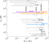 |
Fig. 1. Number of stellar particles equating to the MW-like stellar mass versus the halo mass covered by the simulation. The simulations used for this study are shown in color, with Magneticum Box2 hr shown in blue, TNG100 shown in purple, Horizon-AGN shown in gold, and Hydrangea shown in orange. Other commonly known simulations are shown in gray. Full box cosmological simulations are in light gray, with Mvir, max(z = 0) indicated by a filled circle while the line goes down to the resolution limit of 1000 dark matter particles. Zoom-in simulations are plotted in dark gray, going from the most massive halo in the set (diamond) down to the same 1000 dark matter particle limit (dashed thin line). Vertical dotted lines mark the MW halo mass, the 1014 M⊙ mass threshold used to define clusters, and the Coma cluster mass. Full box simulation suites shown are: Magneticum Pathfinder (Dolag et al. 2025), IllustrisTNG (Nelson et al. 2019b), Horizon-AGN (Dubois et al. 2014), SLOW (Dolag et al. 2023; Seidel et al. 2024), EAGLE (Schaye et al. 2015), Flamingo (Schaye et al. 2023), Millenium-TNG (Pakmor et al. 2023), and Bahamas (McCarthy et al. 2017). Zoom-in simulation suites shown are: Hydrangea (Bahé et al. 2017), Romulus-C (Tremmel et al. 2019), TNG-Clusters (Nelson et al. 2024), Rapsody-G (Hahn et al. 2017), and The300 Project (Cui et al. 2018). |
2.1. Magneticum Pathfinder
For the majority of this work we focus on a set of clusters from the Magneticum Pathfinder1 hydrodynamical cosmological simulations (Dolag et al. 2025), a suite of 6 different simulation volumes with three different resolution levels. For this work, we use in particular Box2 hr, the simulation that has a large volume of (352 cMpc/h)3, with particle masses for dark matter of mdm = 9.8 × 10⁸ M⊙ and for gas of mgas = 2 × 10⁸ M⊙. Because gas particles can spawn up to four generations of stellar particles, the mass resolution in the stellar component is a factor four higher, with masses of m* ≈ mgas/4 ≈ 5 × 10⁷ M⊙, allowing for galaxies of M* ≥ 1010 M⊙ to be sufficiently resolved with 200 stellar particles. Box2 hr harbors a significant number of clusters by z = 0, with 886 galaxy clusters of M200c ≥ 1014 M⊙. The properties of the galaxy clusters from this particular simulation have already been used to study the dynamics of the ICL and BCG components by Remus et al. (2017), and their galaxy populations have been investigated and compared to observations by Lotz et al. (2019, 2021).
The softening lengths for the particle types are ϵdm = ϵgas = 5.3 kpc and ϵ* = 2.84 kpc, while the assumed cosmology is given by WMAP-7 (Komatsu et al. 2011), with h = 0.704, Ωm = 0.272, Ωb = 0.0451, Ωλ = 0.728, σ8 = 0.809 and ns = 0.963. The simulation was performed with a modified version of GADGET-2 (Springel 2005), with upgrades covering the smoothed particle hydrodynamics (SPH), thermal conduction (Dolag et al. 2005) and artificial viscosity (Dolag et al. 2004), among others (Donnert et al. 2013; Beck et al. 2016). The implementation of the baryonic physics is described in more detail by Teklu et al. (2015). We identify galaxies and galaxy clusters using the structure finder SUBFIND (Springel et al. 2001; Dolag et al. 2009). First, a friends-of-friends algorithm identifies linked structures (halos), before saddlepoints in the potential are then used to distinguish the constituent ‘subhalos’. The galaxy which resides at the deepest point in the potential is then defined as the ‘central’, while others are ‘satellites’. The tracing of structures through time requires the building of merger trees that link subhalos (galaxies) from one snapshot (point in time) to the next (see e.g., Srisawat et al. 2013). For Magneticum, we employ L-BASETREE (Springel et al. 2005).
2.2. IllustrisTNG
The Next Generation Illustris2 simulations (IllustrisTNG) are a suite of cosmological hydrodynamical simulations, of which we use the intermediate-sized medium-resolution volume called TNG100 (Marinacci et al. 2018; Naiman et al. 2018; Nelson et al. 2018; Pillepich et al. 2018a; Springel et al. 2018). The simulation has a volume of (75 cMpc/h)3, and particle masses of mdm = 7.5 × 10⁶ M⊙ for the dark matter and m*, gas = 1.4 × 10⁶ M⊙ for the stellar and gas masses. This results in galaxies of M* ≥ 1010 M⊙ to be highly resolved with around 7000 stellar particles. At z = 0, the simulation includes 14 galaxy clusters with masses of M200c ≥ 1014 M⊙. Many previous works have considered both the total stellar content (e.g., Pillepich et al. 2018a) as well as galaxy populations (e.g., Stevens et al. 2019; Donnari et al. 2021) of the simulation galaxy clusters.
For the particle species, the softening lengths are ϵdm = ϵ* = 0.74 kpc, while the spatial resolution of the gas cell is adaptive and is better at higher densities. The assumed cosmology is given by the Planck results (Planck Collaboration XIII 2016), with h = 0.6774, Ωm = 0.3089, Ωb = 0.0486, Ωλ = 0.6911, σ8 = 0.8159 and ns = 0.9667. The simulation was performed with the moving-mesh code AREPO (Springel 2010), with updates as described by Pillepich et al. (2018a,b). Galaxies and galaxy clusters are identified via the structure finder SUBFIND (Springel et al. 2001; Dolag et al. 2009), and structures are linked between snapshots through SUBLINK (Rodriguez-Gomez et al. 2015).
2.3. Horizon-AGN
Horizon-AGN (Dubois et al. 2014) is a cosmological hydrodynamical simulation with a volume of (100 cMpc/h)3, a dark matter particle resolution of mdm = 8 × 10⁷ M⊙, and a stellar particle resolution of m* = 2 × 10⁶ M⊙. This results in galaxies of M* ≥ 1010 M⊙ being well resolved with approximately 5000 stellar particles. At z = 0, the simulation includes 14 galaxy clusters with masses at or just below M200c ≥ 1014 M⊙. Prior work has been done on the buildup of the ICL (Brown et al. 2024), and the shape (Okabe et al. 2018), spin (Choi et al. 2018) and star formation histories of cluster galaxies (Jeon et al. 2022).
The assumed cosmology is given by WMAP-7 (Komatsu et al. 2011), as for Magneticum (i.e., h = 0.704, Ωm = 0.272, Ωb = 0.045, Ωλ = 0.728, σ8 = 0.81 and ns = 0.967). The simulation was performed using the adaptive mesh refinement (AMR)-based Eulerian hydrodynamics code RAMSES (Teyssier 2002). Since the simulation was performed with a grid code, the initially uniform 10243 cell gas grid is refined according to a quasi-Lagrangian criterion, with the smallest cell sizes fixed at 1 physical kpc. For mode details on the technical implementations, see Dubois et al. (2014). We identify galaxies and clusters using the ADAPTAHOP structure finder (Tweed et al. 2009) performed separately on the stars and DM. Structures are identified on the basis of local particle density with no unbinding procedure preformed. Structures and substructures are assembled from the groups created by linking particles with densities greater than 178 and 80 times the total matter density for stars and DM respectively according to their closest local density maxima. ADAPTAHOP then links structures based on saddle points in the density field. The employed merger tree code is TREEMAKER (Tweed et al. 2009).
2.4. Hydrangea
Hydrangea (Bahé et al. 2017, see also Barnes et al. 2017) is a suite of 24 cosmological hydrodynamical zoom-in simulations of massive galaxy clusters using a variant of the EAGLE simulation model (Schaye et al. 2015). The parent simulation has a volume of (2252 cMpc/h)3. The particle resolutions of the Hydrangea clusters are mdm = 9.7 × 10⁶ M⊙ for dark matter, and mgas, * ≈ 1.8 × 10⁶ M⊙, for gas and stars, respectively. This results in galaxies of M* ≥ 1010 M⊙ to be well resolved with ≳6000 stellar particles. Softening lengths are ϵdm = ϵgas = ϵ* = 0.7 kpc, while the assumed cosmology is given by the Planck results (Planck Collaboration XVI 2014), with h = 0.6777, Ωm = 0.307, Ωb = 0.04825, Ωλ = 0.693, σ8 = 0.8288 and ns = 0.9611.
While the parent simulation contains > 105 galaxy clusters, the Hydrangea set of zoom-in simulations contains 46 galaxy clusters with masses above M200c ≥ 1014 M⊙, reaching up to 1015.4 M⊙. We here use all 46 clusters, thus expanding on the set used by Brough et al. (2024). Previous works have shown that the stellar mass function of cluster galaxies in Hydrangea agrees well with observations, both at z ≈ 0 (Bahé et al. 2017) and z ∼ 1 (Ahad et al. 2021). Although star formation in satellites is very efficiently quenched, DM stripping leads to a ≈1 dex positive offset of the stellar-to-halo mass relation from the field (Bahé et al. 2017). As shown by Bahé et al. (2019), only a few per cent of satellite galaxies accreted after z ≈ 2 are fully disrupted. Nevertheless, the simulations predict a substantial ICL component that accounts for ∼20% of the total stellar mass even on group scales (Ahad et al. 2023, see also Brough et al. 2024).
The sub-grid parameters are the same as for the 50 Mpc ‘AGNdT9’ simulation of the EAGLE suite, which differs from the ‘Reference’ model as used for the 100 Mpc EAGLE simulation in the AGN heating temperature increment ΔT and viscosity parameter Cvisc (Schaye et al. 2015). The simulations were performed with a significantly modified version of the SPH code GADGET-3 (last described by Springel 2005). Major updates include the ‘Anarchy’ pressure-entropy SPH scheme (Schaller et al. 2015) as well as subgrid physics models for reionization, gas cooling, star formation, metal enrichment, and stellar and AGN feedback (Schaye et al. 2015), see also Crain et al. 2015). As for TNG100 and Magneticum, we identify galaxies and galaxy clusters via the structure finder SUBFIND (Springel et al. 2001; Dolag et al. 2009), while tracing is done via SPIDERWEB (Bahé et al. 2019).
2.5. Property definitions
Throughout this work, we define our quantities within the radius enclosing 200 times the critical density, R200c. Halo mass is then given as the total mass in that radius, M200c, including also that from satellites. The total stellar mass M*, tot is the sum of all stellar mass in R200c, while the ICL + BCG stellar mass M*, ICL + BCG is the sum of all stellar mass within R200c that is assigned to the central subhalo of the cluster, i.e., excluding mass in satellites. The ratio between the stellar mass in the ICL + BCG to total is given as fICL + BCG = M*, ICL + BCG/M*, tot, and is by definition smaller than unity. Similarly, we only consider satellites whose position lie within R200c of the cluster center (defined by the BCG) when calculating both their stellar mass ratios relative to the BCG, as well as for the total mass in satellite galaxies.
3. Results
As the main goal of this study is to understand to what extent the ICL and the BCG can be used as tracers for the evolution of galaxy clusters, we first investigated the cluster populations with respect to their evolution before we connect them to the ICL and BCG properties. This also provides the basis for comparisons between the different simulations. Unless otherwise noted, we define the halo mass as M200c, which is the total mass within a sphere of mean density of 200 times the critical density.
3.1. Populations of galaxy clusters
Galaxy clusters come in a variety of shapes and sizes, with the usual definition spanning over an order of magnitude in mass from M200c ≥ 1014 M⊙ to > 1015 M⊙. Their differences result from the different assembly histories, with some assembling a majority of their mass already early in the Universe (e.g., Sorce et al. 2020; Remus et al. 2023), while others have only recently undergone major mergers, such as the Coma cluster (e.g., Burns et al. 1994; Sanders et al. 2013; Seidel et al. 2024) or the Abell 2744 cluster (e.g., Owers et al. 2011; Kimmig et al. 2023).
Fig. 2 shows r-band mock images of 20 example galaxy clusters ranging from M200c = 1 × 10¹⁴ M⊙ to M200c ≈ 1.5 × 10¹⁵ M⊙. The clusters are ordered to have increasing M200c from left to right, with clusters in the same column having the same M200c. The rows go from the highest to the lowest BCG mass (top to bottom), where we use M*, 100 kpc, defined as the stellar mass within 100 kpc in 3D, excluding satellites. This is around where Brough et al. (2024) find the transition radius from BCG to ICL to lie for various observational methods (see their Fig. 10). For each cluster, we show the projected image of radius R200c out to a depth of 3 ⋅ R200c. As can be seen immediately, the clusters show a larger amount of diffuse light with increasing halo mass (i.e., from left to right). However, it is also clear that in the galaxy clusters with the highest BCG masses (top row) have relatively less stellar mass (and therefore luminosity) in thesatellites. This implies more recent merging activity for those clusters with lower BCG masses, which is indeed what we find. The galaxy clusters in the bottom rows commonly host two massive galaxies that would make the definition of a single BCG difficult.
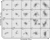 |
Fig. 2. Mock images in the r-band of example galaxy clusters from the Magneticum Box2 hr simulation in a random projection, with increasing mass from left to right and cluster IDs indicated in the top left. Clusters in the left column have about M200c = 1 × 10¹⁴ M⊙, with clusters on the right having M200c > 1 × 10¹⁵ M⊙. From top to bottom we plot galaxy clusters with decreasing BCG stellar mass (within 100 kpc, excising satellites) within a narrow bin of cluster halo mass. Each panel shows the full R200c size of the cluster, with the black line in the bottom left of each panel marking the effective length of 100 kpc while the axes ticks are in units of 0.2r200c. |
As structure merges into the growing cluster, it brings with it a majority of its mass in the form of dark matter, as well as baryons in the form of stars and gas. Depending on the nature of the orbit of the merging galaxies, not all of the stars may reach into the deepest parts of the galaxy cluster potential (Karademir et al. 2019), resulting in a range of stellar masses for the central BCG. This is also the origin for the scatter in the stellar mass-halo mass relation that we show in the left panel of Fig. 3, with a range of around 0.7 dex in M*, 100 kpc at a given halo mass. We note that this scatter is entirely driven by the central BCG + ICL mass, as we exclude any contributions from satellites. For our set of example clusters in Fig. 2, they range in M*, 100 kpc/M200c from 3.4% for cluster ID 925 (top left) to 0.5% for cluster ID 158 (bottom of the third column). Because the higher resolved simulations TNG100, Hydrangea and Horizon-AGN (purple, orange and gold) show a similar scatter in the left panel of Fig. 3, we can conclude this to be inherent in the way mass accretes onto the galaxy clusters. Finally, as also noted by Brough et al. (2024), all simulations reproduce the underlying BCG-halo mass relation (e.g., Brough et al. 2008; Lidman et al. 2012), though there are some differences. Magneticum and Horizon-AGN tend toward higher stellar masses at equivalent halo mass relative to Hydrangea and TNG100, which we believe is likely driven by differences in the implemented subgrid physics. Crucially, however, the slopes of the M* − Mhalo relation are similar.
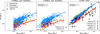 |
Fig. 3. Left: Stellar mass of the central BCG within 100 kpc versus the total halo mass M200c for the four simulations, scaled to a common h. Magneticum is plotted in blue, IllustrisTNG in purple, Hydrangea in orange and Horizon-AGN in gold. Center: Same stellar mass plotted against the halo mass as given by M500c. Also plotted are observations by DeMaio et al. (2018) and Kravtsov et al. (2018). Right: Total stellar mass (BCG, ICL and satellites) against M500c for the simulations, as well as observations by Andreon (2012), Laganá et al. (2013), Gonzalez et al. (2013), Budzynski et al. (2014), Kravtsov et al. (2018), Sartoris et al. (2020). |
To see that this scatter is not due to large fluctuations in the halo mass, which may be driven by recently infalling structure which resides far away from the BCG, we can instead plot M*, 100 kpc against M500c (middle panel of Fig. 3). We find that the range in stellar masses at a given M500c is still significant, and comparable for Magneticum Box2 hr to that found for TNG100. This scatter also matches the ±0.13 dex found by Pillepich et al. (2018a) for TNG300, the larger volume box of the IllustrisTNG suite, with the same galaxy formation model of TNG100. When comparing to individual galaxy cluster observations by DeMaio et al. (2018) and Kravtsov et al. (2018), we find that the simulations tend toward higher stellar masses compared to the observations. We note that we have rescaled all masses to a common h, and that observations at z > 0.2 are plotted in light-gray, which may at least in part be a cause of the differences. The size of the offset may also be mass dependent, where observational measurements for larger clusters could be biased towards lower masses as compared to the simulations (Kravtsov et al. 2018).
In light of recent findings by Popesso et al. (2024), who find Magneticum best reproduces the observed hot gas mass fractions in galaxy clusters, it is interesting to note that Magneticum lies at the highest stellar masses. This may imply the need for even stronger feedback, to neither overproduce the amount of stars nor the amount of hot gas in clusters. Alternatively, given that observations at high redshifts are finding significantly enhanced number densities of quenched galaxies compared to most cosmological simulations (Carnall et al. 2023; Valentino et al. 2023), this may instead indicate the need for an earlier onset of significant AGN feedback (Kimmig et al. 2025).
Notably, the scatter found in the simulations in Fig. 3 is also seen between the individual observations. To see there persists such a variety also for the total stellar content of galaxy clusters, we plot in the right panel of Fig. 3 the total stellar mass in the cluster M*, tot (BCG + ICL + Satellites) against M500c. We find a significant reduction in the scatter for all simulations, as well as closer agreement to observations of individual galaxyclusters by Andreon (2012), Laganá et al. (2013), Gonzalez et al. (2013), Kravtsov et al. (2018), Sartoris et al. (2020). As slopes of the M*, tot-M500c relation, the simulations find 0.96 ± 0.02, 0.86 ± 0.05, 0.84 ± 0.07 and 1.13± for Magneticum, Hydrangea, Horizon-AGN and TNG100, respectively, where it is of note that Pillepich et al. (2018a) find a less steep 0.84 for TNG300. These slopes are comparable to those found by observations, with 0.52 ± 0.04, 1.05 ± 0.05 and 0.69 ± 0.09 found by Gonzalez et al. (2013), Budzynski et al. (2014) and Kravtsov et al. (2018). This could imply either that the larger relative stellar masses in the BCGs found in the simulations result from faster stripping of the satellites, or that the process of masking the satellites in observations also removes a significant amount of stars belonging to the diffuse ICL. Further investigation into this is needed in a more detailed comparison with observations, which will be the focus of a follow-up study to this work.
It is interesting to note, aside from TNG and Budzynski et al. (2014), the slope of the M*, tot-M500c relation lies below that of self-similarity (slope of 1). As we expect the great majority of the stellar mass at the cluster scale to be accreted (e.g., Pillepich et al. 2018a; Remus & Forbes 2022), this may indicate that satellites in smaller clusters of M500c = 1014 M⊙ possess ongoing star formation (e.g., Brown et al. 2024), while the more massive clusters are relatively more efficient in suppressing their satellite galaxies’ star formation. This is consistent with the findings by Lotz et al. (2019), that gas is stripped more quickly in more massive clusters. Alternatively, the infalling regions for lower mass clusters may on average include galaxies that were more efficient at converting gas into stars, so which are potentially earlier formed when the baryon conversion efficiency was higher (Boylan-Kolchin 2023; Turner et al. 2025), as compared to more massive clusters.
We further note that there are considerable differences between individual observations of total stellar versus halo mass. Halo masses based on X-ray gas using hydrostatic assumptions suffer from hydrostatic mass bias (Nelson et al. 2014) while weak-lensing measurements are impacted by weak lensing bias (Grandis et al. 2024). Stellar masses are impacted by uncertain mass-to-light ratios due to the not well known low-mass slope of the initial mass function, as well as a degeneracy between age and metallicity when stellar populations are inferred using broad-band colors (Swindle et al. 2011; Leauthaud et al. 2012).
3.2. Defining cluster dynamical state
Given the large scatter in BCG masses at a given halo mass, we now turn to consider how clusters grow. This means both their average total mass assembly, as well as how much of their stellar mass is already stripped/merged into the BCG or ICL relative to the total amount present.
To do so, we first require a proxy of the mass assembly history. We chose here the formation redshift zform, which is defined as the redshift when the galaxy cluster first reached half of its final halo mass M200c at z = 0. A higher zform means an earlier formation and thus higher degree of relaxation of the galaxy cluster relative to those with lower zform. This is a definition commonly used in the literature (e.g., Boylan-Kolchin et al. 2009; Power et al. 2012, among others). We note that by using zform, we care particularly about the galaxy clusters dynamical evolution through cosmic time and the question of whether a given cluster lived in an early or late collapsing node, and care less about the most recent merging activity. Different definitions of the dynamical state or relaxedness of a galaxy cluster may be better traced by other parameters (Haggar et al. 2024), such as the X-ray center shift, given that the hydrodynamical gas component is stripped and relaxes on faster timescales than the dispersionless stars and dark matter. Indeed, Vallés-Pérez et al. (2023, 2025) find both a timescale and redshift dependence for their dynamical tracers, albeit their simulations exclude star formation and feedback.
Fig. 4 shows the distribution of the formation redshift zform for all clusters from the Magneticum simulations (blue) and the other three simulations. For the large number of Magneticum Box2 hr clusters, we find that the average galaxy cluster assembled half of its mass by a redshift of zform ≈ 0.67, or just over 6 Gyr ago. This is in agreement with previous results for large cosmological dark matter only simulations, where Power et al. (2012) find average formation redshifts of zform ≈ 0.7 for clusters of about Mvir = 1014 M⊙, and of zform ≈ 0.45 for clusters of about Mvir = 1015 M⊙. Similar results are also reported for the Millennium and Millennium-II simulations by Boylan-Kolchin et al. (2009), although these values are slightly older than what is predicted from the Press-Schechter Theorem (see Power et al. 2012).
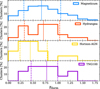 |
Fig. 4. Histograms of the formation redshifts for all clusters from Magneticum Box2 hr (blue), Hydrangea (orange), Horizon-AGN (gold), and TNG100 (purple), going from top to bottom. Median (solid) and 1-σ bounds (dashed) are indicated as vertical lines. |
The range of formation redshifts found for clusters from Magneticum reaches from formation redshifts as early as zform = 1.8 to as late as zform = 0.06. The other simulations used in this work also find a large spread in the formation redshift of their galaxy clusters, despite the lower number statistics of TNG100, Horizon-AGN and Hydrangea, as shown in Fig. 4. The average formation redshift between the samples varies slightly, with the Horizon-AGN clusters being the youngest at ⟨zformHorizon⟩ = 0.44, both Magneticum and Hydrangea at similar formation times with ⟨zformMagneticum⟩ = 0.67 and ⟨zformHydrangea⟩ = 0.71, while TNG100 has the earliest forming clusters at ⟨zformTNG⟩ = 0.78.
We note that both TNG100 and Horizon-AGN lack clusters with zform > 1.4, as well as show a tighter spread. This is likely because they are simulations of about 100 Mpc boxlength and thus lack the largest modes of the initial power spectrum of the density fluctuations (e.g., Remus et al. 2023). As the Magneticum Box2 hr is a factor 3 larger in box-length, this equates to a factor of 27 in volume, and thus it includes not only significantly more galaxy clusters, but also more of the larger modes that can collapse earlier, leading to a larger variety in formation times.
The Hydrangea clusters, meanwhile, are drawn from a very large cosmological parent box of 3200 pMpc boxlength and thus show a similar spread that includes both the earliest and latest forming galaxy clusters. It is interesting that their selection, requiring them to be in relative isolation (no more massive halo within 30 pMpc or 20R200c, whatever is larger), does not seem to imprint in the formation redshifts, unlike what may be typically assumed for more isolated nodes in the cosmic web (see also Remus et al. 2023; Seidel et al. 2024, for more details on this effect of early formation and starvation). Overall, Fig. 4 demonstrates the large variety in formation histories for galaxy clusters, making it a non-trivial problem to distinguish those fromobservations.
3.3. The fraction of ICL + BCG and cluster dynamical state
To get a better understanding of how the mass of these galaxy clusters is assembled, we plot in the upper panels of Fig. 5 the amount of halo mass M200c(z) present in the galaxy clusters of the large Magneticum sample through time, relative to their final halo masses M200c(z = 0). The black line shows the median growth of all clusters, with the dark and light gray shades marking the 1σ- and 2σ-bounds.
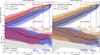 |
Fig. 5. Upper row: Evolution of the halo mass M200, c with redshift z for all clusters in the Magneticum Box2 hr simulation, normalized to the final mass M200, c(z = 0). The black line shows the median, with the dark shaded area marking the 1σ-bounds and the light shaded area marking the 2σ-bounds. The colored lines and their 1σ-bounds show the evolution of a subset of clusters split by their formation redshift (left) or their fICL + BCG (right) as given in the legend. Black dash-dotted vertical lines mark the redshifts at which the average cluster has accumulated 20%, 50%, and 90% of its total mass (horizontal black lines), marked by z20, z50, and z90, respectively. We note that z50 is what we define as formation redshift of a cluster. Lower row: Evolution of fICL + BCG with redshift z. As in the upper panel, the black line marks the average evolution of all clusters from Magneticum, with the gray shaded areas showing the 1σ- and 2σ-bounds. The colored lines and regions show the median and 1σ-bounds for the same subsets of galaxy clusters. |
The overall spread in the histories increases the farther back we look, with the 1σ-bounds reaching 0.5 dex (or a factor of three in range) by z = 1. On one hand, it is remarkable that the relative growth over the last nearly 8 Gyr remains on average within a factor of three for a large sample of clusters that spans well over an order of magnitude in mass at z = 0. On the other hand, by a redshift of z = 1.5 the range of typical progenitors for a M200c = 1014 M⊙ cluster already goes from large galaxies M200c ≈ 7 ⋅ 1012 M⊙ up to intermediate groups M200c ≈ 3 ⋅ 1013 M⊙. Additionally, we note that only the clusters in the upper 2σ-bound actually retain up to 10% of their halo mass down to z = 3, which would place them in the typical range of what is considered a protocluster with M200c > 1 ⋅ 1013 M⊙ (Remus et al. 2023).
To emphasize this point even further, in the upper panel of Fig. 5 we split the total sample (black) into two subsets, those with zform in the upper or lower 1σ-range of the total distribution (red or blue), with the exact cutoff shown in the legend. This results in around 140 clusters for each group. By construction, this results in the largest possible split between the formation redshifts of each group, with those assembling early (red) already reaching 50% of their final halo mass at z ≈ 1.4 (vertical red line), while the late assembling clusters do so only by z ≈ 0.2 (vertical blue line). Interestingly, even though the groups are split based on zform, they are still largely separate at z > 2, indicating that clusters in either group inhabit fundamentally different assembling nodes through cosmic time. This raises the question if there is an observable that could be used to differentiate such starkly diverging histories.
Based on Fig. 3, we know that there is a range in the amount of mass already present in the BCG or ICL, where by contrast the total stellar mass scatters far less for a given halo mass. This is indicative of the mass transfer from satellite galaxies to the BCG or ICL as time passes, due to stripping, merging or other dynamical disruption events.
Therefore, we ask the question whether the mass assembly history of a galaxy cluster can be traced through the fraction of stellar mass contained in the BCG and ICL relative to the total stellar mass, fICL + BCG. We choose this definition instead of only the BCG or the ICL for two reasons. First, there is no clean definition of how to split the ICL from the BCG, as discussed in depth in the literature (see Brough et al. 2024, and discussion therein), with strong disagreement between the kinematic selection and the surface brightness selection methods (see Remus et al. 2017, for a direct comparison). Second, the distribution of stars through different stripping and merging events strongly depends on the orbit of the satellite that is disrupted or merged (Karademir et al. 2019) with the BCG, and as such there are second order effects when considering just the BCG or just the ICL beyond the tracing of dynamical timescales. Finally, though there appear to be two kinematically distinct components in clusters (Remus et al. 2017; Marini et al. 2024), these need not also be physically separate.
We first considered how fICL + BCG evolves with time, plotted in the lower left panel of Fig. 5. The median of the Magneticum clusters is shown as a black solid line and the 1σ and 2σ bounds as dark and light shaded areas, respectively. Overall, fICL + BCG decreases with redshift up to z ≈ 0.6, after which it shows a slight increase again. This increase at later times is interesting when we consider the expectations from the assembly history of dark matter only simulations, where at later times the disruption of substructure occurs on faster timescales (≈1 Gyr) than the accretion of new matter (around 10 Gyr according to Jiang & van den Bosch 2017). In this context, we thus expect an increase in fICL + BCG as more stars are disrupted than new galaxies are accreted. The lowest average value of fICL + BCG is reached at the time when the average cluster has assembled 50% of its mass. This implies that along the history of a galaxy cluster, the time when it has the highest fraction of stellar mass in satellites is when it reaches an intermediate group mass, which we discuss in more detail in Sect. 3.6.
The lower left panel of Fig. 5 also shows the evolution of fICL + BCG for the two subsets split by their zform, where we find a clear difference in their evolution. The early assembling clusters (red) reach their lowest fICL + BCG at z = 1.3, which is comparable to their median zform = 1.25. After this point they grow much slower, taking around 8 Gyrs to assemble the remaining half of their final mass, nearly half of which is spent on the final 10%. Over this same time their fICL + BCG steadily increases up to fICL + BCG = 74% by z = 0, as the clusters grow very slowly with sufficient time to strip and disrupt any accreted satellites. By contrast, the late assembling clusters’ fICL + BCG (blue line in the bottom left panel of Fig. 5) behaves very similar to the total sample of clusters up until z = 0.3, at which point the late assembling clusters sharply drop in fICL + BCG, down to fICL + BCG = 0.45 by z = 0. This coincides with the timeframe where they experience strong total mass growth, more than doubling their halo mass over a time of just around 2 Gyrs.
To confirm the implied anti-correlation between accretion events and fICL + BCG, we also split the sample of clusters based on their fICL + BCG at z = 0. The two groups of around 140 galaxy clusters with the highest/lowest fICL + BCG are shown in the right panels of Fig. 5. We find remarkably similar behavior to when we used the formation redshift to split the clusters, where a high/low fICL + BCG directly implies an earlier/later assembly. What is of particular note is how significantly their mass assembly histories differ, with the 1σ-bounds of the two sets of clusters only overlapping at z = 2. This means that a measurement of fICL + BCG allows us to differentiate the cluster’s mass assembly history over the last 10 Gyrs. Generally, whenever another halo merges into the cluster, fICL + BCG drops as the number of satellite galaxies is increased significantly. After the merger, as long as the cluster stays undisturbed, it starts to disrupt and merge the satellite galaxies, thereby adding the mass to the ICL and the BCG while the cluster is relaxing its dynamical state. However, as we are considering the stellar component which lies in the deepest parts of the satellites’ potential wells, this process is imprinted over long timescales of up to 10 Gyrs. This nicely matches the results by Contreras-Santos et al. (2024) for clusters in The300 Project (Cui et al. 2018), where they find that the amount of ICL increases with the length of time the cluster went without a merger greater than 1:4, from fICL ≈ 20% if the merger was recent, up to 40% if it was at least 10 Gyrs ago.
Fit parameters from the orthogonal distance regression for the relations between various parameters for all four simulations.
3.4. Halo mass (in)dependence
To test whether there is a systematic trend with galaxy cluster mass, we plot fICL + BCG against halo mass M200c in the left panel of Fig. 6. First, we find no clear correlation between the two parameters for any of the simulations. There is a slight tendency of the very most massive clusters with M200c ≈ 1015 M⊙ toward lower fICL + BCG, matching the observed trend (Montes 2022). This is because these clusters generally have formed more recently due to the bottom-up structure formation for a ΛCDM cosmology, and thus had less time to strip their satellites’ stars. However, it is unclear if the simulation volumes probed here are simply too small to house the extreme outlier cases of very early forming galaxy clusters with masses in excess of M200c > 1015 M⊙, which may then exhibit higher fICL + BCG, or if those do not form rapidly enough to be seen by z = 0.
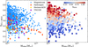 |
Fig. 6. Left panel: Fraction of stellar mass within R200c that is not bound to satellites but instead in the BCG or ICL, fICL + BCG, against the halo mass M200c, for the Magneticum (blue), IllustrisTNG (purple), Horizon-AGN (gold) and Hydrangea (orange) clusters. Right panel: Same as the left panel but for the Magneticum galaxy clusters only, colored by the cluster formation redshift zform. Colors as indicated in the legend. |
We note that we find differences in the absolute values of fICL + BCG between the simulations, with a median fICL + BCG = 0.65, 0.47, 0.46 and 0.55 for Magneticum, Hydrangea, Horizon-AGN and TNG100. On one hand, this may be caused by differences in the implemented subgrid physics, where Popesso et al. (2024) find that Magneticum best reproduces observed cluster gas properties among a set of simulations including IllustrisTNG and EAGLE, but in return produce overly massive central galaxies. On the other hand, the lower resolution of Magneticum could result in a lack of low-mass satellites in galaxy clusters, as they are stripped/disrupted too quickly because of their low particle numbers, which would increase fICL + BCG. Indeed, galaxies of M* < 1010 M⊙ are the progenitors of around 20% of the ICL + BCG stellar mass (Brown et al. 2024). However, as we will show in the following, this does not change the quantitative correlations found between the observables we consider.
When we color the points by the galaxy cluster formation redshift zform in the right panel of Fig. 6, we find a clear color gradient. At a given halo mass M200c, there is a direct correlation between fICL + BCG and zform, where galaxy clusters at the highest (lowest) fICL + BCG have formed the earliest (latest). This provides strong credence to the idea that fICL + BCG can indeed be used as a dynamical clock for the formation of galaxy clusters. We also see this for the different higher-resolved simulations, where, on average, the older galaxy cluster from both TNG100 and Hydrangea (Fig. 4) have higher fICL + BCG than the younger Horizon-AGN clusters (left panel of Fig. 6).
We test this claim in the upper panel of Fig. 7, plotting fICL + BCG at z = 0 against the formation redshift zform of each galaxy cluster from all four simulations. It is apparent that there is a positive correlation, one which is present across all simulations and is therefore stable against calibrations of the subgrid physics. A higher fICL + BCG consistently implies an earlierformation redshift. We quantify this by the Pearson correlation coefficient, finding significant values of p = 0.69, p = 0.72, p = 0.82 and p = 0.83 for Magneticum, Hydrangea, Horizon-AGN and TNG100, respectively. We have tested and find similar correlation strengths for both the Spearman (p > 0.68) and Kendall rank coefficients (p > 0.5), which is to be expected given that there is not strong indication away from linearity between fICL + BCG and zform. Furthermore, Contreras-Santos et al. (2024) also found fICL to correlate significantly with zform for The300 clusters, while Yoo et al. (2024) show in their Fig. 4 that for massive groups and clusters at z = 0.6 in Horizon Run 5 (Lee et al. 2021) the link to the formation time is driven primarily by the BCG, rather than the ICL.
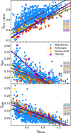 |
Fig. 7. Upper panel:fICL + BCG versus formation redshift zform, for the galaxy clusters from the Magneticum (blue), TNG100 (purple), Horizon-AGN (gold), and Hydrangea simulations (orange). The gray box displays the Pearson correlation coefficient for each simulation between fICL + BCG and zform. The closer the absolute value is to unity, the tighter the correlation. We further include best fit lines for each simulation determined via the least squares method (colored lines). Middle panel: Center shift between the 3D gas barycenter and the location of the BCG (normalized by R200c), plotted as a function of the formation redshift, with the colors the same as the upper panel. Lower panel: Fraction of the total halo mass mass which is in all subhalos fsub (so excluding the central and diffuse halo) versus formation redshift, with colors as in the upper two panels. |
The lower two panels of Fig. 7 show two other common tracers of the dynamical state of galaxy clusters known from the literature, namely the gas center shift sgas (middle panel) and the fraction of total mass (including DM) in subhalos fsub (lower panel), for all simulations. The former is given by the distance offset between the location of the BCG (typically at the deepest point in the potential) and the barycenter of all gas within R200c. We normalize this offset then by R200c. Larger values thus indicate a strongly disturbed distribution of gas compared to the underlying dark matter halo, indicative of recent merging activity (e.g., Biffi et al. 2016; Zenteno et al. 2020; Kimmig et al. 2023).
As expected from previous works, both sgas and fsub trace the formation redshift. However, we find for all simulations that fICL + BCG correlates tighter (or comparably well) with zform compared to established dynamical state tracers, allowing for a better overall predictive power. This again matches what is found by Yoo et al. (2024) on the lower mass, higher redshift end (massive groups and small clusters at z = 0.6), that fICL + BCG is as tight or tighter than the centershift or subhalo total mass fraction. We compile the best fit lines for each simulation for the formation redshift zform as a function of fICL + BCG, sgas and fsub in Table 1. We fit via orthogonal distance regression, which minimizes the errors in both directions, and provide the fit parameters in Table 1 (for a discussion on the predictive power of the fit compared to least-squares fitting, we refer to the Appendix A).
3.5. Tracing ICL + BCG through other observables
As the ICL is difficult to observe even with the upcoming facilities, one question that remains is in how well the fraction of stars in the ICL plus BCG can be approximated by measuring other observables. In Fig. 8 we show four parameters that are generally easier to obtain than the stellar mass in the BCG and ICL itself. From left to right, we show the correlations between fICL + BCG and 1) the stellar mass ratio between the BCG and the second most massive galaxy within R200c of the cluster, M12 ≡ M*, BCG/M*, 2nd, also termed the fossilness parameter (Tremaine & Richstone 1977; Loh & Strauss 2006; Ragagnin et al. 2017); 2) the stellar mass ratio between the BCG and the fourth most massive galaxy in the cluster, M14 (Golden-Marx & Miller 2018); 3) the normalized offset sstars = Δr/R200c between the barycenter of stellar mass of the cluster within R200c and the position of the BCG, also known as the center shift (Mann & Ebeling 2012; Biffi et al. 2016; Contreras-Santos et al. 2022); and 4) the quantity ϕBCG = M*, BCG/R*, 1/2, BCG in units of M⊙/kpc, an approximation for the central stellar potential depth following Bluck et al. (2023), where we determine the stellar mass M*, BCG and stellar half-mass radius R*, 1/2, BCG for the BCG within 0.1 ⋅ R200c.
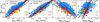 |
Fig. 8. Comparison of fICL + BCG against different dynamical tracers for all individual clusters from Magneticum Box2 (blue), TNG100 (purple), Horizon-AGN (gold), and Hydrangea (orange). The numbers in each panel indicate the Pearson correlation coefficient found for each relation and simulation (colors). We plot fICL + BCG against the stellar mass ratio of the BCG to the second (left panel) and fourth (second panel) most massive galaxy inside the cluster, counting the BCG. The third panel shows fICL + BCG as a function of the offset between the stellar barycenter and the BCG position sstars, while the right panel plots the fraction against the stellar potential ϕstars = M*/R*, half determined within 0.1 ⋅ R200c. |
Across all four simulations (Magneticum in blue, TNG100 in purple, Horizon-AGN in gold, and Hydrangea in orange) we consistently find that the correlation between fICL + BCG and the two stellar mass ratios (M12 and M14) is tightest, with remarkably little scatter. The Pearson correlation coefficients are shown in the figure, with all simulations finding p ≥ 0.7. Interestingly, while there appears to be an offset between the simulations in the relation between fICL + BCG and M12, there is much less for the correlation between fICL + BCG and M14. This could imply that the fourth most massive galaxy is a more consistent representative of the overall stripping that occurred in the cluster, where the second most massive galaxy may be less affected. Nonetheless, we find that fICL + BCG may be well determined by both M12 and M14 for all simulations, with very similar slopes in the best fit lines for all, the values of which we provide in Table 1. When considering the relations of fICL + BCG to sstars and in particular to ϕBCG, we find significantly increased scatter. For the latter, aside from Magneticum, the simulations find little to no correlation.
This means that good measurements of satellite stellar masses as well as the BCG (including, however, identifying cluster membership) are sufficient to tightly determine the overall fraction of stellar mass in the ICL and BCG fICL + BCG. That fraction, in turn, well captures the mass assembly history of a galaxy cluster. Most significantly, we find this correlation to be stable against changes in the subgrid physics as well as the choice of structure finder. However, we note that when we test the partial correlation between zform and both M12 and M14, we find that the underlying driver is their correlation with fICL + BCG. Consequently, using the mass ratios to predict a cluster’s zform will generally add scatter compared to directly using fICL + BCG. This point is further discussed in Appendix A.
We then broaden the spectrum of galaxy cluster parameters to also include a) the center shift of the gaseous component sgas, that is the offset between the BCG and the barycenter of the gas, closely mimicking the X-ray determined center shift (see Appendix B); b) the fraction of total mass contained in the 8th most massive substructure f8 (see Kimmig et al. 2023, for more details), and both the total number (i.e., cluster richness) as well as passive fraction fquench of cluster galaxies with M* > 1010 M⊙ (e.g., Aguerri et al. 2006). The full matrix of correlations between all these different tracers of the dynamical state of a cluster is shown in Fig. 9.
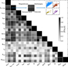 |
Fig. 9. Full matrix of the correlation strength between different parameters, with darker colors indicating stronger correlations, for all four simulations as indicated at the respective tiles for each panel. From top to bottom and left to right are the same parameters, in the following order: formation redshift zform, the fraction of stellar mass within ICL plus BCG fICL + BCG, the center shift between the stellar (sstars) or gas barycenter (sgas) and the BCG, the fraction of total mass within all substructures fsub or within just the 8th most massive substructure f8, the stellar mass ratio between the BCG and the second (M12) or fourth (M14) most massive galaxy in a cluster, the central stellar potential ϕBCG, the passive fraction fquench of galaxies in the cluster with stellar masses above 1 × 10¹⁰ M⊙ as well as their total number Nsat, and the total halo mass M200c. We note that black squares in the diagonal mark the self-correlation of the parameters and are thus all equal to one. |
Fig. 9 is structured as follows: for a given parameter we determine the Pearson correlation strength with another parameter, doing this for every simulation separately to fill a two-by-two grid, with Magneticum in the upper left, Hydrangea in the upper right, Horizon-AGN in the lower left and finally TNG100 in the lower right. We color the cell based on the strength, going from white (p = 0, no correlation) to black (p = 1, one-to-one correlation). The upper inset of Fig. 9 illustrates this process for the case of a correlation between fICL + BCG versus zform. We note that the full black squares in the top diagonal mark the relation between a parameter and itself, and are thus all fully black (p = 1).
The first column in Fig. 9 shows the correlation strength between the formation redshift zform with all other parameters, for each of the simulations. We find that the overall strongest correlation exists for fICL + BCG, aside from Hydrangea where fsub performs negligibly better (p = 0.74 versus p = 0.72). Matching what is found by Kimmig et al. (2023), all simulations find f8 to be a good tracer for fsub (though weaker for Horizon-AGN). This is the dark matter equivalent to how the mass ratios M12 and M14 trace fICL + BCG (see the second column of Fig. 9 or Fig. 8), and thus, for all simulations, M12 and M14 also strongly correlate with zform. fICL + BCG remains the true, tighter underlying correlation, however, as we discuss in Appendix A.
For all simulations, the number of satellite galaxies with stellar masses above 1010 M⊙, Nsat correlates significantly with the total halo mass M200c, as expected. What is interesting is that the simulations do not find a significant correlation between the halo mass M200c and the formation redshift zform, aside from TNG100. For that simulation, however, M200c also shows a notable correlation with fICL + BCG, which may be the more fundamental link given that this is what the other three simulations find. Indeed, when we consider partial correlations, we find also for TNG100 that the correlation between zform and M200c practically vanishes when accounting for fICL + BCG, as we discuss inAppendix A.
Finally, we find that the fraction of quenched galaxies fq is only weakly correlated with any other parameter (except for Hydrangea), which is likely because most of the galaxies in these massive clusters at low redshifts are simply quenched in all simulations. Interestingly, the gas centershift sgas, while also tracing the formation redshift (see Fig. 7), does not correlate as strongly with the magnitude gaps or fICL + BCG, which may indicate that it traces a different kind of dynamical state due to the collisional nature of the gas.
Thus, we conclude that the formation time of galaxy clusters, defined as the time when a cluster has assembled half of its present-day mass, is best traced through the present-day distribution of stellar mass, which in turn likely has to do with how this matter is stripped (or not) from satellites. This is best quantified by how much of the total stellar mass is bound to the full potential of the cluster, i.e., the BCG and the ICL, or in second order through the stellar mass ratios between the BCG and the most massive companion galaxies.
3.6. Evolution through cosmic time
Finally, we want to understand the origin of the correlation between the stellar mass contained in the ICL plus BCG, and the formation redshift of galaxy clusters. As we are interested in the statistical behavior now, we will restrict the analysis in this last subsection to the Magneticum Box2 hr simulation only. To that end, we plot again the stellar-mass halo-mass relation in Fig. 10, but this time for all stars in R200c (gray), as well as the subset of those stars which are not bound in satellites, and so belong to the BCG or ICL (colored). As already seen for all simulations in the right panel of Fig. 3, the total stellar mass is tightly increasing with halo mass, following a slope very close to 1.
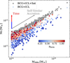 |
Fig. 10. Stellar mass-halo mass relation for the Magneticum Box2 hr clusters. The gray points show the total stellar mass within R200c, including the BCG, ICL and satellites. The colored symbols show the stellar mass of only the ICL and the BCG together, without including satellite galaxies. These points are colored according to the formation redshift of the cluster from older and more relaxed galaxy clusters (red) to younger, recently assembled clusters (blue). |
On the other hand, the colored points which exclude the mass in satellites show a much larger scatter, with a slightly flatter slope. There is a clear color gradient driving this scatter, however, which is given by the formation redshift of the galaxy cluster. Clusters that have nearly all of their stellar mass in the BCG or ICL are consistently older and more relaxed, while clusters with lower BCG + ICL masses are more recently formed. As expected from Fig. 6, this is independent of halo mass. Consequently, if a cluster has time to disrupt and merge their satellite galaxies without being disturbed by additional merging, they will do so consistently across a full order of magnitude in halo mass. This demonstrates why fICL + BCG is such an effective clock for tracing the formation time, and mirrors prior results in the EAGLE simulations on the group mass scale by Matthee et al. (2017). Similar results were also found by Ragagnin et al. (2022), who explicitly find zform to correlate with the location of a cluster in the stellar mass-halo mass relation. When using the concentration of the halo as a proxy for the assembly time, this furthermore agrees with the recent works by Montenegro-Taborda et al. (2025) for TNG300 and Contini et al. (2024a) for a semi-analytic model, who find that clusters with a higher fraction of stellar mass in their (BCG and) ICL are more compact and thus earlier assembling. In the latter case, they find that the scatter in their fICL − Mhalo relation is driven by the halo concentration.
We use this fact to split our sample of 868 galaxy clusters into two further groups. In ten equally log-spaced halo mass bins going from M200c = 1014 M⊙ to M200c = 5 × 10¹⁴ M⊙ we select the 5 galaxy cluster with the highest/lowest fICL + BCG. Using these two samples of 50 clusters each, which represent the extreme ends in fICL + BCG at a given halo mass, we trace the evolution in the distribution of stellar mass between the BCG (red), ICL (gold), second most massive satellite (violet) and the remaining satellites (blue) in Fig. 11. We choose here to define the split between BCG and ICL at 0.1 × R200c, which allows the split to vary with the scale of the halo over time. For further definitions including a fixed aperture cut, we refer to Fig. B.2 in the appendix, and simply note here that the qualitative results do not change strongly depending on the definition of the split.
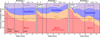 |
Fig. 11. Fraction of the total stellar mass contained in the different components of the Magneticum Box2 hr galaxy clusters versus time, determined for all clusters (left panel) and for the 50 clusters with the highest (central panel) and the 50 clusters with the lowest fICL + BCG for their halo mass (right panel). The fraction of stellar mass contained within the BCG is shown in red, while the fraction in the ICL, the second most massive satellite, and all other satellites are plotted in gold, violet and blue, respectively. The black vertical lines mark the times when the median mass of each group of galaxy clusters is M200, cri > 1 × 10¹³ M⊙ (dotted), M200, cri > 5 × 10¹³ M⊙ (dashed), and M200, cri > 1 × 10¹⁴ M⊙ (dash-dotted). We note that here we split the BCG and ICL at 0.1 × R200, cri. For different definitions of the split between the ICL and the BCG, see Fig. B.2 in the Appendix. |
First, we consider in the left panel of Fig. 11 the evolution in the components for all 868 clusters, where we take the fractions in each component and calculate their mean. We find that while the progenitors of the clusters were in the group mass regime (z ≈ 2, given by the dotted vertical black line) the central galaxy dominated the overall stellar component, accounting for anywhere from 40% to 70%. As they grow from groups to clusters by z = 0.5 (dash-dotted line), the fraction of total stellar mass contained in satellites (second most massive plus others) increases, even while the amount of ICL increases too. This is because the BCG does not grow as quickly in stellar mass as satellites are accreted onto the cluster over this time. Upon reaching galaxy cluster masses, the BCG accounts for just 40% of total stellar mass, with the fraction in ICL rising to 20%. The second most massive galaxy at this point contains 15% of the galaxy cluster stellar mass, which is down from the group regime where it accounted for up to 20%. Consequently, as the overall contribution of satellites has increased this stellar mass is now distributed across a greater number of galaxies as opposed to being dominated by a single massive satellite. Finally, by z = 0, the fraction in ICL has continued rising to 25%, this time drawing from both the BCG as well as the satellites, following a rate of growth comparable to that found by Rudick et al. (2011). This is reasonable as it becomes more difficult for less massive infalling satellites to penetrate deeply into the growing galaxy cluster potential, and they are instead stripped already farther out (Lotz et al. 2019).
When we consider the subset of galaxy clusters with the highest fICL + BCG, we find generally similar behavior. The crucial difference is that these processes occur much earlier, as their progenitors are already groups at z = 3 and would thus fulfill the definition of what is typically considered a protocluster (Remus & Forbes 2022). By z = 1, they are already galaxy clusters, though with some differences to what we found for the total sample. They are more dominated by their BCG, which contains around half of the stellar mass (versus 40%), at the cost of both the ICL at 15% (versus 20%) and the satellites at 35% (versus 40%). This means at the moment these early forming clusters reach halo masses M200c > 1014 M⊙, they are already more centrally concentrated compared to the average clusters. Down to z = 0 their BCGs actually increase in stellar mass fraction (up to 53%), as does their ICL (up to 30%). This is because they strip, disrupt or merge with a significant portion of their satellites, given the nearly 6 Gyr time they have to do so, and by z = 0 their second most massive satellite barely accounts for 5% of the total stellar mass.
Finally, for the sample of clusters with the lowest fICL + BCG, we note first that although they reach group masses at a similar time to the total sample (at z = 1.9 vs. z = 2.3), they stagnate significantly afterwards. By z = 0.5, when the average galaxy cluster progenitor has reached halo masses M200c > 1014 M⊙, the progenitors of clusters with the lowest fICL + BCG are barely above massive groups. Indeed, it takes another nearly 2 Gyr of additional time until they reach galaxy cluster mass. At that time their BCG accounts for just 35% of the total stellar mass, while their ICL is about 15%. Indeed, their satellites already dominate the overall stellar mass at nearly half, which only increases toward z = 0 and ends at around 60% of their total stellar mass bound in satellites. The second most massive satellite is at a comparable stellar mass fraction to the BCG, at 25%. We therefore see here how the present-day distribution of stellar mass within galaxy clusters tightly reflects their differing, distinct mass assembly histories over cosmic time.
3.7. Rate of satellite shredding
Thus, one interesting question that arises is how fast a cluster can disrupt its satellites to add their mass to the ICL + BCG. To this end, we consider how the halo mass and fICL + BCG change together over a characteristic time T. We choose T = 1 Gyr as it is approximately equal to the typical crossing time of our galaxy clusters (Jiang & van den Bosch 2016; Contreras-Santos et al. 2022; Haggar et al. 2024), though we tested that our conclusions do not strongly depend on varying the timescale between T = 0.5 Gyr to T = 2 Gyr. Defining t1 as the starting point and t2 as the end of the window, then
 (1)
(1)
 (2)
(2)
In Fig. 12 we plot ΔfICL + BCG against δM200c based on the assembly histories of our 868 galaxy clusters. The columns show the relation at z > 0.8 (left), 0.8 > z > 0.2 (center) and z < 0.2 (right), based on the redshift at the end of the time window t2. We further split the sample based on the halo mass at the time t2, plotting all clusters’ assembly histories (top row), or only those clusters where the main progenitor has a halo mass of a small group 1 × 10¹³ M⊙ ≤ M200c < 5 × 10¹³ M⊙ (second row), massive group 5 × 10¹³ M⊙ ≤ M200c < 1 × 10¹⁴ M⊙ (third row), or is already a cluster 1 × 10¹⁴ M⊙ ≤ M200c (bottom row). We plot the median and 1σ-bounds (solid and dashed thick black lines), as well as the horizontal and vertical lines corresponding to a net change of zero in either mass or fICL + BCG.
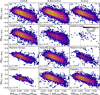 |
Fig. 12. Absolute change in fICL + BCG versus the relative change in mass δM200c as determined over a period of T = 1 Gyr for the Magneticum clusters. Columns from left to right split the sample into redshift bins, while the rows separate the clusters based on their current mass, going from all clusters in the top row to small and massive groups and finally clusters on the bottom row. The median line and 1σ-bounds are plotted in black, while the thin vertical and horizontal black lines show the location of zero change in either fICL + BCG or cluster mass. y0 indicated in each panel is the median change in fICL + BCG for halos where the total mass did not change, δM200c = 0. |
Beginning with the top row, we find a negative dependence of ΔfICL + BCG on δM200c. When the halo mass decreases, δM200c < 0, then ΔfICL + BCG is most positive, which means that fICL + BCG most strongly increases. This may be the result of either a fly-by or a merger. For the former, a structure had previously entered the halo, bringing with it also stellar mass, and has then exited again. Because both halo and satellite stellar mass are removed, δM200c < 0 and ΔfICL + BCG > 0. For the latter, this is a consequence of the definition of M200c. As a structure begins to merge, increasingly more mass of the infalling satellite lies within the radial definition of R200c, until a peak M200c is reached that is approximately the sum of both structures total mass. However, if it is massive enough, the infalling structure does not instantly merge, instead continuing on its orbit until it reaches the apocenter. At this point, a portion of its mass may again lie outside of R200c, thus decreasing M200c (and increasing fICL + BCG as satellite stellar mass is moved outside of the cluster extent).
When the halo mass does not change over T = 1 Gyr, δM200c = 0, then ΔfICL + BCG ≈ 4%. Thus, if left alone these systems increase the fraction of the total stellar mass contained within the BCG and ICL over time, consistent with the picture of stripping and merging. Finally, when δM200c > 0, so when the halo grows, then ΔfICL + BCG is either close to zero or negative. During large accretion events involving significant total mass, the fraction of the stellar mass in satellites therefore also increases (so fICL + BCG decreases).
What is remarkable is that the median line of this behavior remains consistent both across time (left to right columns) as well as between structures of different masses (top to bottom rows). This may indicate that there is an average response between the distribution of the stellar mass and the growth (or lack thereof) of the halo mass of the structure. Generally, as can be seen from the color indicating the number of systems, most lie in the lower right quadrant where they are experiencing slight growth in halo mass while fICL + BCG decreases as they continue to accrete more satellites over time. Simultaneously, there is also a large amount of systems in the upper right, experiencing slow and steady mass growth while still efficiently disrupting their satellites enough to overall increase their fICL + BCG.
We defined the average change in fICL + BCG when a structure does not grow (δM200c = 0) as the “shredding rate” and indicate this value in the panels of Fig. 12. We find that for galaxy groups ΔfICL + BCG ≈ 4%, while galaxy clusters lie slightly lower at 3% to 4% per Gyr. Therefore, as long as there is no new material being accreted, the stellar mass in the ICL + BCG will increase by around 4% of the galaxy cluster total stellar mass. Slower disruption rates of galaxies in clusters compared to groups were also found by Bahé et al. (2019), consistent with our findings here. We note that there is a relatively large scatter for individual clusters, as the actual rate of course depends on various factors. If the cluster is already strongly dominated by the BCG and ICL, then the remaining galaxies may be on more circular orbits that are stripped less quickly, while a cluster post major merger may suddenly and significantly increase its fICL + BCG when the two constituent BCGs merge. Indeed, Fig. 12 shows that there are also clusters at z < 0.2 which increase fICL + BCG by 20% while δM200c = 0, which likely has to do with the orbits, masses, compactness and velocity of the satellite population.
4. Summary and conclusions
To inform the upcoming large surveys of galaxy clusters, which will provide a plethora of data on the largest forming structures throughout time, we have analyzed the buildup of the BCG and the ICL through four separate simulations. We have studied the connection between the fraction of the stellar mass in the ICL + BCG of clusters, fICL + BCG, and their formation histories, following up on initial ideas presented by Brough et al. (2024), and show that this fraction acts as a dynamical clock for galaxy clusters. We primarily employed Box2 hr of the Magneticum Pathfinder hydrodynamical simulation suite (Dolag et al., in prep.), which has a box volume of (352 cMpc/h)3 and 886 galaxy clusters with halo masses M200c > 1014 M⊙, of which we considered 868 here. We complemented this statistical sample with a smaller sample of higher resolved galaxy clusters from the TNG100 (Pillepich et al. 2018a) and Horizon-AGN (Dubois et al. 2014) simulations (14 clusters each), as well as from the Hydrangea suite of zoom-in cluster simulations (Bahé et al. 2017, 46 clusters), to verify that the results found for Magneticum are independent of the resolution, numerical details, or subgrid physics prescriptions.
Defining the formation redshift zform of galaxy clusters as the redshift when the cluster first assembled 50% of its z = 0 halo mass, we find that clusters in Magenticum Box2 hr have on average assembled only recently with ⟨zformBox2⟩ = 0.67, in agreement with previous studies (e.g., Boylan-Kolchin et al. 2009; Power et al. 2012), but that some clusters already assembled as early as zform = 1.8. This is consistent with the non-linearity in the growth of individual clusters compared to their statistical average and is matched nicely by linear growth theory (see also Remus et al. 2023 and Kimmig et al., in prep.).
Here, it is of special interest to note that there is a difference in cluster formation times, with the (on average) latest forming clusters in Horizon-AGN at ⟨zformHorizon⟩ = 0.44, Magneticum and Hydrangea are similar at ⟨zformMagneticum⟩ = 0.67 and ⟨zformHydrangea⟩ = 0.71, while TNG100 has the earliest forming clusters at ⟨zformTNG⟩ = 0.78. However, all simulations cover a similar range in formation redshifts (Fig. 4), so that we can meaningfully compare the higher resolved simulations of TNG100, Horizon-AGN and Hydrangea to the larger sample of clusters in Magneticum Box2 hr.
We find that the formation time of a galaxy cluster zform is tightly traced by fICL + BCG, so the fraction of total stellar mass within the ICL + BCG (Fig. 7), complementing what was found by Yoo et al. (2024) for massive groups and clusters at z = 0.6. We show this follows because the stripping/merging of stellar mass bound in satellite galaxies into the central potential of a galaxy cluster is proportional to how long a cluster has been left undisturbed (Fig. 12, see also Contreras-Santos et al. 2024). More relaxed clusters have higher fractions of fICL + BCG, with values up to 90%, while recent accretion can (temporarily) push the fraction down to as low as 20% (Fig. 6). This is mirrored in other complementary studies that find fICL to trace the formation time of clusters, such as Contreras-Santos et al. (2024) for The300 project, or for the SAM by Contini et al. (2024a) who used the halo concentration as a proxy to zform (Ragagnin et al. 2019).
We found that this time dependence on the stripping efficacy is also the origin for the scatter in the BCG stellar mass-halo mass relation (Fig. 3). Galaxy clusters at the upper end in stellar mass formed much earlier and are thus both more compact and had more time to disrupt and strip their satellite populations (Fig. 10), which is again in agreement with other such simulation findings (Ragagnin et al. 2022; Contini et al. 2024a) and in support of observational works that find this scatter correlates with dynamical tracers such as M14 (Golden-Marx & Miller 2018; Golden-Marx et al. 2025). If left undisturbed, that is to say without growing their halo mass, galaxy clusters will gradually disrupt their satellite population, stripping most or all of their mass even if a small core may survive. We calculated an average rate for this “shredding”, finding it to be between 3% and 4% of the total stellar mass in the cluster per Gyr (Fig. 12).
We considered two other common tracers of the dynamical state, namely the fraction of total mass (including DM) in the galaxy cluster’s subhalos, fsub, and the gas center shift sgas, defined as the offset between the 3D gas barycenter and the BCG position. Across all four simulations, fICL + BCG best traces zform (Fig. 7). This is likely because different dynamical tracers trace different dynamical times, as shown by Haggar et al. (2024). In the future, a more detailed investigation in the timescales involved for the gas (X-ray centershift) and dark matter stripping (fsub) is necessary to understand when to use which tracer (Vallés-Pérez et al. 2023, 2025), to inform the new and upcoming measurements from multiple instruments that will significantly improve the set of observed galaxy clusters, such as Euclid (Laureijs et al. 2011; Kluge et al. 2025), Roman (Montes et al. 2023) and Rubin/LSST (Ivezić et al. 2019; Brough et al. 2020). However, that is beyond the scope of this work. Instead, we provide here fitting functions to predict the formation redshift zform of observed galaxy clusters from measurements of fICL + BCG (Table 1). This may complement machine learning approaches to predict zform from various observables (Srivastava et al. 2025).
We show that fICL + BCG, which is difficult to measure because of the low surface brightness of the outer ICL, can best be approximated by the stellar mass ratio between the BCG and the second or fourth most massive galaxy, M12 or M14 (Fig. 8), in agreement with Golden-Marx et al. (2025). Furthermore, all four simulations agree remarkably well on the presented relations, even though they are tuned to reproduce different relations, with Magneticum in particular focused on the hot gas component (Popesso et al. 2024). This is likely because the processes of stripping and merging for the stellar component of galaxy clusters is driven by gravity, which is treated equivalently between the simulations. We provide fitting functions from each simulation to estimate fICL + BCG based on M12, M14, the stellar barycenter offset sstars and the ratio of BCG stellar mass to half mass radius ϕstars (Table 1). Finally, we determine that, although M12 and M14 well trace zform for all simulations, the underlying driver of the correlation is fICL + BCG (Fig. 9). Accurate measurements of the low surface brightness ICL of galaxy clusters are thus necessary to best predict galaxy cluster assembly.
We conclude that the assembly histories of galaxy clusters are varied and complex, but that their present-day properties hold the key to disentangling their evolution. With the increasing number of massive galaxies observed by JWST, finding a means to robustly connect the largest cosmic structures through time is becoming increasingly necessary. This study finds that the distribution of the stellar component of these clusters, quantified either via the fraction of the total stellar mass in the ICL + BCG fICL + BCG or alternatively the stellar mass ratios of the BCG to the second or fourth most massive galaxy in the cluster, M12 or M14, is a crucial tool to predict whether a cluster originates from an early or late collapsing node of the cosmic web. Therefore, despite the difficulty of measuring this low surface brightness feature of galaxy clusters, it is of great importance as the field of galaxy cluster research moves into the next phase with statistically significant samples from our observed Universe.
Data availability
The Magneticum Pathfinder simulation data are available at https://c2papcosmosim.uc.lrz.de/ (Ragagnin et al. 2017), with larger data sets on request.
The Hydrangea simulation data are publicly available at https://ftp.strw.leidenuniv.nl/bahe/Hydrangea/
The Horizon-AGN data used in this work can be obtained upon request from https://www.horizon-simulation.org/data.html
The IllustrisTNG data used in this work are publicly available at http://www.tng-project.org
Acknowledgments
LCK acknowledges support by the Deutsche Forschungsgemeinschaft (DFG, German Research Foundation) under project nr. 516355818. SB acknowledges funding support from the Australian Research Council through a Discovery Project DP190101943. KD and LCK acknowledge support for the COMPLEX project from the European Research Council (ERC) under the European Union’s Horizon 2020 research and innovation program grant agreement ERC-2019-AdG 882679. LCK, KD and RSR acknowledge support by DFG under Germany’s Excellence Strategy – EXC-2096 – 3900783311. YMB acknowledges support from UK Research and Innovation through a Future Leaders Fellowship (grant agreement MR/X035166/1) and financial support from the Swiss National Science Foundation (SNSF) under project 200021_213076. GM and NH are supported by STFC consolidated grant ST/X000982/1. MM acknowledges support from grant RYC2022-036949-I financed by the MICIU/AEI/10.13039/501100011033 and by ESF+ and program Unidad de Excelencia María de Maeztu CEX2020-001058-M. HJB gratefully acknowledges support from the UK Science and Technology Facilities Council (STFC) under grant ST/Y509437/1. AE acknowledges funding by the CNES post-doctoral fellowship program. Y.J-T. acknowledges financial support from the State Agency for Research of the Spanish MCIU through Center of Excellence Severo Ochoa award to the Instituto de Astrofísica de Andalucía CEX2021-001131-S funded by CIN/AEI/10.13039/501100011033, and from the grant PID2022-136598NB-C32 Estallidos and project ref. AST22-00001-Subp-15 funded from the EU-NextGenerationEU. R.R. acknowledges financial support through grants PRIN-MIUR 2020SKSTHZ and through INAF-WEAVE StePS founds. MS acknowledges the support by the Italian Ministry for Education University and Research (MIUR) grant PRIN 2022 2022383WFT “SUNRISE”, CUP C53D23000850006 and by VST funds. Co-funded by the European Union (MSCA Doctoral Network EDUCADO, GA 101119830 and Widening Participation, ExGal-Twin, GA 101158446). JHK acknowledges Spanish grant PID2022-136505NB-I00 funded by MCIN/AEI/10.13039/501100011033 and EU, ERDF. This work used the DiRAC@Durham facility managed by the Institute for Computational Cosmology on behalf of the STFC DiRAC HPC Facility (www.dirac.ac.uk). The equipment was funded by BEIS capital funding via STFC capital grants ST/K00042X/1, ST/P002293/1 and ST/R002371/1, Durham University and STFC operations grant ST/S003908/1. DiRAC is part of the National e-Infrastructure. The Magneticum simulations were performed at the Leibniz-Rechenzentrum with CPU time assigned to the Project pr83li. We are especially grateful for the support by M. Petkova through the Computational Center for Particle and Astrophysics (C2PAP). The Horizon-AGN simulations were undertaken using the HPC resources of CINES under the allocations 2013047012, 2014047012 and 2015047012 made by GENCI and were partially supported by grant Spin(e) (ANR-13-BS05-0005, https://www.cosmicorigin.org/). This work has made use of the Horizon cluster on which the simulation was post-processed, hosted by the Institut d’Astrophysique de Paris. Part of the analysis of the simulations was carried out on the DiRAC Facility jointly funded by BIS and STFC. We warmly thank S. Rouberol for running it smoothly. The IllustrisTNG simulations were undertaken with compute time awarded by the Gauss Centre for Supercomputing (GCS) under GCS Large-Scale Projects GCS-ILLU and GCS-DWAR on the GCS share of the supercomputer Hazel Hen at the High Performance Computing Center Stuttgart (HLRS), as well as on the machines of the Max Planck Computing and Data Facility (MPCDF) in Garching, Germany. This research was supported by the International Space Science Institute (ISSI) in Bern, through ISSI International Team project number 23-577.
References
- Aguerri, J. A. L., Castro-Rodríguez, N., Napolitano, N., Arnaboldi, M., & Gerhard, O. 2006, A&A, 457, 771 [NASA ADS] [CrossRef] [EDP Sciences] [Google Scholar]
- Ahad, S. L., Bahé, Y. M., Hoekstra, H., van der Burg, R. F. J., & Muzzin, A. 2021, MNRAS, 504, 1999 [CrossRef] [Google Scholar]
- Ahad, S. L., Bahé, Y. M., & Hoekstra, H. 2023, MNRAS, 518, 3685 [Google Scholar]
- Ahvazi, N., Sales, L. V., Navarro, J. F., et al. 2024, Open J. Astrophys., 7, 111 [CrossRef] [Google Scholar]
- Aldás, F., Zenteno, A., Gómez, F. A., et al. 2023, MNRAS, 525, 1769 [CrossRef] [Google Scholar]
- Andreon, S. 2012, A&A, 548, A83 [NASA ADS] [CrossRef] [EDP Sciences] [Google Scholar]
- Bahé, Y. M., Barnes, D. J., Dalla Vecchia, C., et al. 2017, MNRAS, 470, 4186 [Google Scholar]
- Bahé, Y. M., Schaye, J., Barnes, D. J., et al. 2019, MNRAS, 485, 2287 [Google Scholar]
- Barnes, D. J., Kay, S. T., Bahé, Y. M., et al. 2017, MNRAS, 471, 1088 [Google Scholar]
- Beck, A. M., Murante, G., Arth, A., et al. 2016, MNRAS, 455, 2110 [Google Scholar]
- Bender, R., Kormendy, J., Cornell, M. E., & Fisher, D. B. 2015, ApJ, 807, 56 [Google Scholar]
- Biffi, V., Borgani, S., Murante, G., et al. 2016, ApJ, 827, 112 [NASA ADS] [CrossRef] [Google Scholar]
- Bilata-Woldeyes, B., Perea, J. D., & Solanes, J. M. 2025, A&A, 695, A234 [NASA ADS] [CrossRef] [EDP Sciences] [Google Scholar]
- Bluck, A. F. L., Piotrowska, J. M., & Maiolino, R. 2023, ApJ, 944, 108 [NASA ADS] [CrossRef] [Google Scholar]
- Boylan-Kolchin, M. 2023, Nat. Astron., 7, 731 [NASA ADS] [CrossRef] [Google Scholar]
- Boylan-Kolchin, M., Springel, V., White, S. D. M., Jenkins, A., & Lemson, G. 2009, MNRAS, 398, 1150 [Google Scholar]
- Brambila, D., Lopes, P. A. A., Ribeiro, A. L. B., & Cortesi, A. 2023, MNRAS, 523, 785 [NASA ADS] [CrossRef] [Google Scholar]
- Brough, S., Couch, W. J., Collins, C. A., et al. 2008, MNRAS, 385, L103 [NASA ADS] [CrossRef] [Google Scholar]
- Brough, S., Tran, K. V., Sharp, R. G., von der Linden, A., & Couch, W. J. 2011, MNRAS, 414, L80 [Google Scholar]
- Brough, S., Collins, C., Demarco, R., et al. 2020, ArXiv e-prints [arXiv:2001.11067] [Google Scholar]
- Brough, S., Ahad, S. L., Bahé, Y. M., et al. 2024, MNRAS, 528, 771 [NASA ADS] [CrossRef] [Google Scholar]
- Brown, H. J., Martin, G., Pearce, F. R., et al. 2024, MNRAS, 534, 431 [NASA ADS] [CrossRef] [Google Scholar]
- Budzynski, J. M., Koposov, S. E., McCarthy, I. G., & Belokurov, V. 2014, MNRAS, 437, 1362 [Google Scholar]
- Burke, C., Hilton, M., & Collins, C. 2015, MNRAS, 449, 2353 [Google Scholar]
- Burns, J. O., Roettiger, K., Ledlow, M., & Klypin, A. 1994, ApJ, 427, L87 [Google Scholar]
- Canepa, L., Brough, S., Lanusse, F., Montes, M., & Hatch, N. 2025, ApJ, 980, 245 [Google Scholar]
- Carnall, A. C., McLeod, D. J., McLure, R. J., et al. 2023, MNRAS, 520, 3974 [NASA ADS] [CrossRef] [Google Scholar]
- Casas, M. C., Putnam, K., Mantz, A. B., Allen, S. W., & Somboonpanyakul, T. 2024, ApJ, 967, 14 [Google Scholar]
- Choi, H., Yi, S. K., Dubois, Y., et al. 2018, ApJ, 856, 114 [Google Scholar]
- Chon, G., Böhringer, H., & Zaroubi, S. 2015, A&A, 575, L14 [NASA ADS] [CrossRef] [EDP Sciences] [Google Scholar]
- Chun, K., Shin, J., Ko, J., Smith, R., & Yoo, J. 2024, ApJ, 969, 142 [Google Scholar]
- Conroy, C., Wechsler, R. H., & Kravtsov, A. V. 2007, ApJ, 668, 826 [NASA ADS] [CrossRef] [Google Scholar]
- Contini, E., De Lucia, G., Villalobos, Á., & Borgani, S. 2014, MNRAS, 437, 3787 [Google Scholar]
- Contini, E., Yi, S. K., & Kang, X. 2018, MNRAS, 479, 932 [NASA ADS] [Google Scholar]
- Contini, E., Jeon, S., Rhee, J., Han, S., & Yi, S. K. 2023, ApJ, 958, 72 [NASA ADS] [CrossRef] [Google Scholar]
- Contini, E., Rhee, J., Han, S., Jeon, S., & Yi, S. K. 2024a, AJ, 167, 7 [NASA ADS] [CrossRef] [Google Scholar]
- Contini, E., Yi, S. K., & Jeon, S. 2024b, ArXiv e-prints [arXiv:2404.01560] [Google Scholar]
- Contreras-Santos, A., Knebe, A., Pearce, F., et al. 2022, MNRAS, 511, 2897 [NASA ADS] [CrossRef] [Google Scholar]
- Contreras-Santos, A., Knebe, A., Cui, W., et al. 2024, A&A, 683, A59 [NASA ADS] [CrossRef] [EDP Sciences] [Google Scholar]
- Crain, R. A., Schaye, J., Bower, R. G., et al. 2015, MNRAS, 450, 1937 [NASA ADS] [CrossRef] [Google Scholar]
- Cui, W., Power, C., Borgani, S., et al. 2017, MNRAS, 464, 2502 [NASA ADS] [CrossRef] [Google Scholar]
- Cui, W., Knebe, A., Yepes, G., et al. 2018, MNRAS, 480, 2898 [Google Scholar]
- Da Rocha, C., Ziegler, B. L., & Mendes de Oliveira, C. 2008, MNRAS, 388, 1433 [Google Scholar]
- Davison, T. A., Norris, M. A., Pfeffer, J. L., Davies, J. J., & Crain, R. A. 2020, MNRAS, 497, 81 [Google Scholar]
- De Lucia, G., & Blaizot, J. 2007, MNRAS, 375, 2 [Google Scholar]
- DeMaio, T., Gonzalez, A. H., Zabludoff, A., et al. 2018, MNRAS, 474, 3009 [Google Scholar]
- Dolag, K., Jubelgas, M., Springel, V., Borgani, S., & Rasia, E. 2004, ApJ, 606, L97 [NASA ADS] [CrossRef] [Google Scholar]
- Dolag, K., Vazza, F., Brunetti, G., & Tormen, G. 2005, MNRAS, 364, 753 [NASA ADS] [CrossRef] [Google Scholar]
- Dolag, K., Borgani, S., Murante, G., & Springel, V. 2009, MNRAS, 399, 497 [Google Scholar]
- Dolag, K., Murante, G., & Borgani, S. 2010, MNRAS, 405, 1544 [NASA ADS] [Google Scholar]
- Dolag, K., Sorce, J. G., Pilipenko, S., et al. 2023, A&A, 677, A169 [NASA ADS] [CrossRef] [EDP Sciences] [Google Scholar]
- Dolag, K., Remus, R.-S., Valenzuela, L. M., et al. 2025, ArXiv e-prints [arXiv:2504.01061] [Google Scholar]
- Donahue, M., Connor, T., Fogarty, K., et al. 2015, ApJ, 805, 177 [Google Scholar]
- Donnari, M., Pillepich, A., Joshi, G. D., et al. 2021, MNRAS, 500, 4004 [Google Scholar]
- Donnert, J., Dolag, K., Brunetti, G., & Cassano, R. 2013, MNRAS, 429, 3564 [Google Scholar]
- Dubois, Y., Pichon, C., Welker, C., et al. 2014, MNRAS, 444, 1453 [Google Scholar]
- Dubois, Y., Peirani, S., Pichon, C., et al. 2016, MNRAS, 463, 3948 [Google Scholar]
- Edwards, L. O. V., Alpert, H. S., Trierweiler, I. L., Abraham, T., & Beizer, V. G. 2016, MNRAS, 461, 230 [Google Scholar]
- Edwards, L. O. V., Salinas, M., Stanley, S., et al. 2020, MNRAS, 491, 2617 [Google Scholar]
- Edwards, L. O. V., Hamel, K. A. S. J., Shy, J. C., et al. 2024, MNRAS, 530, 3924 [Google Scholar]
- Ellien, A., Slezak, E., Martinet, N., et al. 2021, A&A, 649, A38 [NASA ADS] [CrossRef] [EDP Sciences] [Google Scholar]
- Feldmeier, J. J., Mihos, J. C., Morrison, H. L., et al. 2004, ApJ, 609, 617 [Google Scholar]
- Fu, H., Shankar, F., Ayromlou, M., et al. 2024, MNRAS, 532, 177 [NASA ADS] [CrossRef] [Google Scholar]
- Furnell, K. E., Collins, C. A., Kelvin, L. S., et al. 2021, MNRAS, 502, 2419 [NASA ADS] [CrossRef] [Google Scholar]
- Giallongo, E., Menci, N., Grazian, A., et al. 2014, ApJ, 781, 24 [Google Scholar]
- Golden-Marx, J. B., & Miller, C. J. 2018, ApJ, 860, 2 [NASA ADS] [CrossRef] [Google Scholar]
- Golden-Marx, J. B., Zhang, Y., Ogando, R. L. C., et al. 2025, MNRAS, 538, 622 [Google Scholar]
- Gonzalez, A. H., Zaritsky, D., & Zabludoff, A. I. 2007, ApJ, 666, 147 [Google Scholar]
- Gonzalez, A. H., Sivanandam, S., Zabludoff, A. I., & Zaritsky, D. 2013, ApJ, 778, 14 [Google Scholar]
- Grandis, S., Ghirardini, V., Bocquet, S., et al. 2024, A&A, 687, A178 [NASA ADS] [CrossRef] [EDP Sciences] [Google Scholar]
- Haggar, R., Gray, M. E., Pearce, F. R., et al. 2020, MNRAS, 492, 6074 [NASA ADS] [CrossRef] [Google Scholar]
- Haggar, R., De Luca, F., De Petris, M., et al. 2024, MNRAS, 532, 1031 [Google Scholar]
- Hahn, O., Martizzi, D., Wu, H.-Y., et al. 2017, MNRAS, 470, 166 [NASA ADS] [Google Scholar]
- Iodice, E., Capaccioli, M., Grado, A., et al. 2016, ApJ, 820, 42 [Google Scholar]
- Ito, K., Valentino, F., Brammer, G., et al. 2024, ApJ, 964, 192 [CrossRef] [Google Scholar]
- Ivezić, Ž., Kahn, S. M., Tyson, J. A., et al. 2019, ApJ, 873, 111 [Google Scholar]
- Jauzac, M., Eckert, D., Schwinn, J., et al. 2016, MNRAS, 463, 3876 [NASA ADS] [CrossRef] [Google Scholar]
- Jeon, S., Yi, S. K., Dubois, Y., et al. 2022, ApJ, 941, 5 [Google Scholar]
- Jiang, F., & van den Bosch, F. C. 2016, MNRAS, 458, 2848 [NASA ADS] [CrossRef] [Google Scholar]
- Jiang, F., & van den Bosch, F. C. 2017, MNRAS, 472, 657 [NASA ADS] [CrossRef] [Google Scholar]
- Jiménez-Teja, Y., Dupke, R., Benítez, N., et al. 2018, ApJ, 857, 79 [Google Scholar]
- Jiménez-Teja, Y., Vílchez, J. M., Dupke, R. A., et al. 2021, ApJ, 922, 268 [CrossRef] [Google Scholar]
- Jiménez-Teja, Y., Dupke, R. A., Lopes, P. A. A., & Vílchez, J. M. 2023, A&A, 676, A39 [NASA ADS] [CrossRef] [EDP Sciences] [Google Scholar]
- Jiménez-Teja, Y., Dupke, R. A., Lopes, P. A. A., & Dimauro, P. 2024, ApJ, 960, L7 [CrossRef] [Google Scholar]
- Jones, L. R., Ponman, T. J., Horton, A., et al. 2003, MNRAS, 343, 627 [NASA ADS] [CrossRef] [Google Scholar]
- Joo, H., & Jee, M. J. 2023, Nature, 613, 37 [NASA ADS] [CrossRef] [Google Scholar]
- Joo, H., Jee, M. J., Kim, J., et al. 2024, ApJ, submitted [arXiv:2411.08117] [Google Scholar]
- Karademir, G. S., Remus, R.-S., Burkert, A., et al. 2019, MNRAS, 487, 318 [Google Scholar]
- Khochfar, S., & Burkert, A. 2003, ApJ, 597, L117 [Google Scholar]
- Kimmig, L. C., Remus, R.-S., Dolag, K., & Biffi, V. 2023, ApJ, 949, 92 [Google Scholar]
- Kimmig, L. C., Remus, R.-S., Seidel, B., et al. 2025, ApJ, 979, 15 [Google Scholar]
- Kluge, M., Neureiter, B., Riffeser, A., et al. 2020, ApJS, 247, 43 [Google Scholar]
- Kluge, M., Bender, R., Riffeser, A., et al. 2021, ApJS, 252, 27 [Google Scholar]
- Kluge, M., Hatch, N. A., Montes, M., et al. 2025, A&A, 697, A13 [NASA ADS] [CrossRef] [EDP Sciences] [Google Scholar]
- Komatsu, E., Smith, K. M., Dunkley, J., et al. 2011, ApJS, 192, 18 [Google Scholar]
- Kravtsov, A. V., Vikhlinin, A. A., & Meshcheryakov, A. V. 2018, Astron. Lett., 44, 8 [Google Scholar]
- Laganá, T. F., Martinet, N., Durret, F., et al. 2013, A&A, 555, A66 [NASA ADS] [CrossRef] [EDP Sciences] [Google Scholar]
- Laureijs, R., Amiaux, J., Arduini, S., et al. 2011, ArXiv e-prints [arXiv:1110.3193] [Google Scholar]
- Leauthaud, A., George, M. R., Behroozi, P. S., et al. 2012, ApJ, 746, 95 [Google Scholar]
- Lee, J., Shin, J., Snaith, O. N., et al. 2021, ApJ, 908, 11 [CrossRef] [Google Scholar]
- Libeskind, N. I., van de Weygaert, R., Cautun, M., et al. 2018, MNRAS, 473, 1195 [NASA ADS] [CrossRef] [Google Scholar]
- Lidman, C., Suherli, J., Muzzin, A., et al. 2012, MNRAS, 427, 550 [Google Scholar]
- Loh, Y.-S., & Strauss, M. A. 2006, MNRAS, 366, 373 [Google Scholar]
- Longobardi, A., Arnaboldi, M., Gerhard, O., & Hanuschik, R. 2015, A&A, 579, A135 [NASA ADS] [CrossRef] [EDP Sciences] [Google Scholar]
- Lotz, M., Remus, R.-S., Dolag, K., Biviano, A., & Burkert, A. 2019, MNRAS, 488, 5370 [NASA ADS] [CrossRef] [Google Scholar]
- Lotz, M., Dolag, K., Remus, R.-S., & Burkert, A. 2021, MNRAS, 506, 4516 [NASA ADS] [CrossRef] [Google Scholar]
- Mann, A. W., & Ebeling, H. 2012, MNRAS, 420, 2120 [NASA ADS] [CrossRef] [Google Scholar]
- Mao, T.-X., Wang, J., Frenk, C. S., et al. 2018, MNRAS, 478, L34 [Google Scholar]
- Marinacci, F., Vogelsberger, M., Pakmor, R., et al. 2018, MNRAS, 480, 5113 [NASA ADS] [Google Scholar]
- Marini, I., Saro, A., Borgani, S., & Boi, M. 2024, A&A, 689, A181 [NASA ADS] [CrossRef] [EDP Sciences] [Google Scholar]
- Martin, G., Bazkiaei, A. E., Spavone, M., et al. 2022, MNRAS, 513, 1459 [NASA ADS] [CrossRef] [Google Scholar]
- Martin, G., Pearce, F. R., Hatch, N. A., et al. 2024, MNRAS, 535, 2375 [Google Scholar]
- Martínez-Lombilla, C., Brough, S., Montes, M., et al. 2023, MNRAS, 518, 1195 [Google Scholar]
- Matthee, J., Schaye, J., Crain, R. A., et al. 2017, MNRAS, 465, 2381 [NASA ADS] [CrossRef] [Google Scholar]
- McBride, J., Fakhouri, O., & Ma, C.-P. 2009, MNRAS, 398, 1858 [NASA ADS] [CrossRef] [Google Scholar]
- McCarthy, I. G., Schaye, J., Bird, S., & Le Brun, A. M. C. 2017, MNRAS, 465, 2936 [Google Scholar]
- Mihos, J. C. 2004, in Clusters of Galaxies: Probes of Cosmological Structure and Galaxy Evolution, eds. J. S. Mulchaey, A. Dressler, & A. Oemler, 277 [Google Scholar]
- Mihos, J. C., Harding, P., Feldmeier, J., & Morrison, H. 2005, ApJ, 631, L41 [Google Scholar]
- Mihos, J. C., Harding, P., Feldmeier, J. J., et al. 2017, ApJ, 834, 16 [Google Scholar]
- Mittal, R., Whelan, J. T., & Combes, F. 2015, MNRAS, 450, 2564 [Google Scholar]
- Monaco, P., Murante, G., Borgani, S., & Fontanot, F. 2006, ApJ, 652, L89 [Google Scholar]
- Montenegro-Taborda, D., Rodriguez-Gomez, V., Pillepich, A., et al. 2023, MNRAS, 521, 800 [NASA ADS] [CrossRef] [Google Scholar]
- Montenegro-Taborda, D., Avila-Reese, V., Rodriguez-Gomez, V., Manuwal, A., & Cervantes-Sodi, B. 2025, MNRAS, 537, 3954 [Google Scholar]
- Montes, M. 2022, Nat. Astron., 6, 308 [NASA ADS] [CrossRef] [Google Scholar]
- Montes, M., & Trujillo, I. 2014, ApJ, 794, 137 [Google Scholar]
- Montes, M., & Trujillo, I. 2018, MNRAS, 474, 917 [Google Scholar]
- Montes, M., Brough, S., Owers, M. S., & Santucci, G. 2021, ApJ, 910, 45 [Google Scholar]
- Montes, M., Annibali, F., Bellazzini, M., et al. 2023, ArXiv e-prints [arXiv:2306.09414] [Google Scholar]
- Murante, G., Arnaboldi, M., Gerhard, O., et al. 2004, ApJ, 607, L83 [NASA ADS] [CrossRef] [Google Scholar]
- Murante, G., Giovalli, M., Gerhard, O., et al. 2007, MNRAS, 377, 2 [Google Scholar]
- Naiman, J. P., Pillepich, A., Springel, V., et al. 2018, MNRAS, 477, 1206 [Google Scholar]
- Nelson, K., Lau, E. T., Nagai, D., Rudd, D. H., & Yu, L. 2014, ApJ, 782, 107 [NASA ADS] [CrossRef] [Google Scholar]
- Nelson, D., Pillepich, A., Springel, V., et al. 2018, MNRAS, 475, 624 [Google Scholar]
- Nelson, D., Pillepich, A., Springel, V., et al. 2019a, MNRAS, 490, 3234 [Google Scholar]
- Nelson, D., Springel, V., Pillepich, A., et al. 2019b, Comput. Astrophys. Cosmol., 6, 2 [Google Scholar]
- Nelson, D., Pillepich, A., Ayromlou, M., et al. 2024, A&A, 686, A157 [NASA ADS] [CrossRef] [EDP Sciences] [Google Scholar]
- Neto, A. F., Gao, L., Bett, P., et al. 2007, MNRAS, 381, 1450 [NASA ADS] [CrossRef] [Google Scholar]
- Okabe, T., Nishimichi, T., Oguri, M., et al. 2018, MNRAS, 478, 1141 [NASA ADS] [CrossRef] [Google Scholar]
- Oliva-Altamirano, P., Brough, S., Lidman, C., et al. 2014, MNRAS, 440, 762 [NASA ADS] [CrossRef] [Google Scholar]
- Oliva-Altamirano, P., Brough, S., Jimmy, Kim-Vy, T., et al. 2015, MNRAS, 449, 3347 [CrossRef] [Google Scholar]
- Owers, M. S., Randall, S. W., Nulsen, P. E. J., et al. 2011, ApJ, 728, 27 [Google Scholar]
- Pakmor, R., Springel, V., Coles, J. P., et al. 2023, MNRAS, 524, 2539 [NASA ADS] [CrossRef] [Google Scholar]
- Pillepich, A., Nelson, D., Hernquist, L., et al. 2018a, MNRAS, 475, 648 [Google Scholar]
- Pillepich, A., Springel, V., Nelson, D., et al. 2018b, MNRAS, 473, 4077 [Google Scholar]
- Planck Collaboration XIII. 2016, A&A, 594, A13 [NASA ADS] [CrossRef] [EDP Sciences] [Google Scholar]
- Planck Collaboration XVI. 2014, A&A, 571, A16 [NASA ADS] [CrossRef] [EDP Sciences] [Google Scholar]
- Popesso, P., Marini, I., Dolag, K., et al. 2024, A&A, submitted [arXiv:2411.17120] [Google Scholar]
- Power, C., Knebe, A., & Knollmann, S. R. 2012, MNRAS, 419, 1576 [NASA ADS] [CrossRef] [Google Scholar]
- Puchwein, E., Springel, V., Sijacki, D., & Dolag, K. 2010, MNRAS, 406, 936 [NASA ADS] [Google Scholar]
- Ragagnin, A., Dolag, K., Biffi, V., et al. 2017, Astron. Comput., 20, 52 [Google Scholar]
- Ragagnin, A., Dolag, K., Moscardini, L., Biviano, A., & D’Onofrio, M. 2019, MNRAS, 486, 4001 [Google Scholar]
- Ragagnin, A., Andreon, S., & Puddu, E. 2022, A&A, 666, A22 [NASA ADS] [CrossRef] [EDP Sciences] [Google Scholar]
- Ragusa, R., Spavone, M., Iodice, E., et al. 2021, A&A, 651, A39 [NASA ADS] [CrossRef] [EDP Sciences] [Google Scholar]
- Ragusa, R., Mirabile, M., Spavone, M., et al. 2022, Front. Astron. Space Sci., 9, 852810 [CrossRef] [Google Scholar]
- Ragusa, R., Iodice, E., Spavone, M., et al. 2023, A&A, 670, L20 [NASA ADS] [CrossRef] [EDP Sciences] [Google Scholar]
- Raouf, M., Smith, R., Khosroshahi, H. G., et al. 2019, ApJ, 887, 264 [NASA ADS] [CrossRef] [Google Scholar]
- Reefe, M., McDonald, M., Chatzikos, M., et al. 2025, ApJ, submitted [arXiv:2501.08527] [Google Scholar]
- Remus, R.-S., & Forbes, D. A. 2022, ApJ, 935, 37 [NASA ADS] [CrossRef] [Google Scholar]
- Remus, R.-S., Dolag, K., & Hoffmann, T. 2017, Galaxies, 5, 49 [NASA ADS] [CrossRef] [Google Scholar]
- Remus, R.-S., Dolag, K., & Dannerbauer, H. 2023, ApJ, 950, 191 [NASA ADS] [CrossRef] [Google Scholar]
- Rennehan, D., Babul, A., Hayward, C. C., et al. 2020, MNRAS, 493, 4607 [NASA ADS] [CrossRef] [Google Scholar]
- Roberts, I. D., Parker, L. C., & Hlavacek-Larrondo, J. 2018, MNRAS, 475, 4704 [NASA ADS] [CrossRef] [Google Scholar]
- Rodriguez-Gomez, V., Genel, S., Vogelsberger, M., et al. 2015, MNRAS, 449, 49 [Google Scholar]
- Rodriguez-Gomez, V., Pillepich, A., Sales, L. V., et al. 2016, MNRAS, 458, 2371 [Google Scholar]
- Rudick, C. S., Mihos, J. C., & McBride, C. 2006, ApJ, 648, 936 [NASA ADS] [CrossRef] [Google Scholar]
- Rudick, C. S., Mihos, J. C., Frey, L. H., & McBride, C. K. 2009, ApJ, 699, 1518 [Google Scholar]
- Rudick, C. S., Mihos, J. C., & McBride, C. K. 2011, ApJ, 732, 48 [Google Scholar]
- Sanders, J. S., Fabian, A. C., Churazov, E., et al. 2013, Science, 341, 1365 [Google Scholar]
- Santucci, G., Brough, S., Scott, N., et al. 2020, ApJ, 896, 75 [NASA ADS] [CrossRef] [Google Scholar]
- Sartoris, B., Biviano, A., Rosati, P., et al. 2020, A&A, 637, A34 [NASA ADS] [CrossRef] [EDP Sciences] [Google Scholar]
- Schaller, M., Frenk, C. S., Bower, R. G., et al. 2015, MNRAS, 451, 1247 [Google Scholar]
- Schaye, J., Crain, R. A., Bower, R. G., et al. 2015, MNRAS, 446, 521 [Google Scholar]
- Schaye, J., Kugel, R., Schaller, M., et al. 2023, MNRAS, 526, 4978 [NASA ADS] [CrossRef] [Google Scholar]
- Schwinn, J., Baugh, C. M., Jauzac, M., Bartelmann, M., & Eckert, D. 2018, MNRAS, 481, 4300 [Google Scholar]
- Seidel, B. A., Dolag, K., Remus, R.-S., et al. 2024, A&A, submitted [arXiv:2412.08708] [Google Scholar]
- Shaw, L. D., Weller, J., Ostriker, J. P., & Bode, P. 2006, ApJ, 646, 815 [NASA ADS] [CrossRef] [Google Scholar]
- Sorce, J. G., Gottlöber, S., & Yepes, G. 2020, MNRAS, 496, 5139 [NASA ADS] [CrossRef] [Google Scholar]
- Spavone, M., Capaccioli, M., Napolitano, N. R., et al. 2017, A&A, 603, A38 [NASA ADS] [CrossRef] [EDP Sciences] [Google Scholar]
- Spavone, M., Iodice, E., van de Ven, G., et al. 2020, A&A, 639, A14 [NASA ADS] [CrossRef] [EDP Sciences] [Google Scholar]
- Spavone, M., Iodice, E., Lohmann, F. S., et al. 2024, A&A, 689, A306 [NASA ADS] [CrossRef] [EDP Sciences] [Google Scholar]
- Springel, V. 2005, MNRAS, 364, 1105 [Google Scholar]
- Springel, V. 2010, MNRAS, 401, 791 [Google Scholar]
- Springel, V., Yoshida, N., & White, S. D. M. 2001, New Astron., 6, 79 [Google Scholar]
- Springel, V., White, S. D. M., Jenkins, A., et al. 2005, Nature, 435, 629 [Google Scholar]
- Springel, V., Pakmor, R., Pillepich, A., et al. 2018, MNRAS, 475, 676 [Google Scholar]
- Srisawat, C., Knebe, A., Pearce, F. R., et al. 2013, MNRAS, 436, 150 [NASA ADS] [CrossRef] [Google Scholar]
- Srivastava, A., Cui, W., de Andres, D., et al. 2025, ArXiv e-prints [arXiv:2504.14426] [Google Scholar]
- Stevens, A. R. H., Diemer, B., Lagos, C. d. P., et al. 2019, MNRAS, 483, 5334 [NASA ADS] [CrossRef] [Google Scholar]
- Swindle, R., Gal, R. R., La Barbera, F., & de Carvalho, R. R. 2011, AJ, 142, 118 [NASA ADS] [CrossRef] [Google Scholar]
- Teklu, A. F., Remus, R.-S., Dolag, K., et al. 2015, ApJ, 812, 29 [Google Scholar]
- Teyssier, R. 2002, A&A, 385, 337 [CrossRef] [EDP Sciences] [Google Scholar]
- Tremaine, S. D., & Richstone, D. O. 1977, ApJ, 212, 311 [NASA ADS] [CrossRef] [Google Scholar]
- Tremblay, G. R., O’Dea, C. P., Baum, S. A., et al. 2015, MNRAS, 451, 3768 [Google Scholar]
- Tremmel, M., Quinn, T. R., Ricarte, A., et al. 2019, MNRAS, 483, 3336 [CrossRef] [Google Scholar]
- Turner, C., Tacchella, S., D’Eugenio, F., et al. 2025, MNRAS, 537, 1826 [NASA ADS] [CrossRef] [Google Scholar]
- Tweed, D., Devriendt, J., Blaizot, J., Colombi, S., & Slyz, A. 2009, A&A, 506, 647 [NASA ADS] [CrossRef] [EDP Sciences] [Google Scholar]
- Valentino, F., Brammer, G., Gould, K. M. L., et al. 2023, ApJ, 947, 20 [NASA ADS] [CrossRef] [Google Scholar]
- Vallés-Pérez, D., Planelles, S., Monllor-Berbegal, Ó., & Quilis, V. 2023, MNRAS, 519, 6111 [CrossRef] [Google Scholar]
- Vallés-Pérez, D., Planelles, S., & Quilis, V. 2025, A&A, 699, A1 [NASA ADS] [CrossRef] [EDP Sciences] [Google Scholar]
- Véliz Astudillo, S., Carrasco, E. R., Nilo Castellón, J. L., Zenteno, A., & Cuevas, H. 2025, A&A, 693, A106 [NASA ADS] [CrossRef] [EDP Sciences] [Google Scholar]
- Yoo, J., Park, C., Sabiu, C. G., et al. 2024, ApJ, 965, 145 [Google Scholar]
- Zenteno, A., Hernández-Lang, D., Klein, M., et al. 2020, MNRAS, 495, 705 [Google Scholar]
- Zhang, Y., Golden-Marx, J. B., Ogando, R. L. C., et al. 2024, MNRAS, 531, 510 [Google Scholar]
- Zibetti, S., White, S. D. M., Schneider, D. P., & Brinkmann, J. 2005, MNRAS, 358, 949 [Google Scholar]
Appendix A: Partial correlations and fitting
Given that in Fig. 7 we find fICL + BCG to tightly trace the cluster formation redshift zform, it is of relevance if this correlation is driven by some other parameter that provides the link. To test the true driver of the relation to zform, we calculate the partial correlation to fICL + BCG while accounting for all other parameters considered in this study individually. The partial correlation between two parameters x and y, accounting for z, is determined by fitting two linear regressions: between x and z as well as y and z. The residuals in x and y of these fits are thus corrected for any possible correlation with z, and the Pearson correlation coefficient of these residuals is defined as the partial correlation coefficient, which we plot in Fig. A.1. In all cases and for all simulations, the correlation between zform and fICL + BCG remains significantly in place. Indeed, aside from fsub for Hydrangea, the correlation of any parameter (from magnitude gap to center shift to halo mass) with zform is less significant once accounting for that parameters correlation with fICL + BCG. While it is possible that there is another underlying driver which best determines a galaxy cluster’s formation redshift, of all the parameters discussed in this study, fICL + BCG is the strongest.
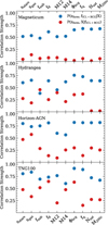 |
Fig. A.1. Partial correlation of zform with fICL + BCG, accounting for other parameters X (blue), or between zform and X, accounting for fICL + BCG (red), for all four simulations (panels). |
This correlation allowed us to define a fitting function, using fICL + BCG to predict zform, as discussed for Fig. 7. In the top row of Fig. A.2 we show the best fit lines between zform and fICL + BCG, as well as to sgas and fsub, by using either the least-squares method, reducing the errors in either the x (red) or y-direction (blue), as well as using orthogonal distance regression (black, ODR), where both axes are weighted equally over the full range of their data. Using these best fit lines, we calculate the predicted formation redshift zform, prediction and plot the cumulative distribution in absolute offset between the prediction and true zform in the bottom row of Fig. A.2. The average 1σ-error is given by the vertical colored lines.
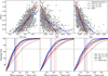 |
Fig. A.2. Top row: The Magneticum data as in Fig. 7, with the axes swapped. Solid lines show the best fits using either the least-squares method, fitting toward x (red) or y (blue), as well as the best fit using orthogonal distance regression (black). Bottom row: Cumulative histogram of the absolute offset between the predicted versus actual formation redshifts for the three best fit lines, as well as when drawing randomly from a normal distribution of formation redshifts with the mean and standard deviation calculated from the total sample of clusters (gray). The 1σ-bounds (68.27%) are shown as colored vertical lines. |
We find that the least-squares fit in the direction of x to y produces the overall tightest predictions, as expected because it minimizes precisely this error. ODR performs nearly as well in all cases, and additionally accounts for errors in the x-direction. As such, we chose ODR when calculating the best fit parameters defined in Table 1. We note that of all three dynamical tracers, fICL + BCG performs the best in predicting zform, with a 1σ-error of around ±0.25. While this is not insignificant, it is still remarkable that the time when a galaxy cluster had first assembled half of its present day total mass is imprinted into the current stellar distribution of mass to the point of being able to predict that time with just a 30% error on average (given the median zform = 0.67). The greatest deviations occur for galaxy clusters which assembled very recently (low zform) but which already have merged most of that stellar mass into the BCG or ICL (high fICL + BCG). For these cases, we find that it can be useful to consider other dynamical tracers as well, as often the center shift in the gas or stars still shows that there was a recent merger, even if the overall stars have already become bound to the central halo.
Appendix B: Definitions for center shift and BCG versus ICL
There are different options when defining a center shift, the offset between what represents the deepest point of the potential, traced either via the BCG or peak in the X-ray surface brightness, and the larger scale barycenter, either of the stellar mass, light, gas mass or X-ray luminosity. We chose for our comparison the BCG as the first point, and then determined the offset relative to the three-dimensional barycenter of the stellar (sstars) or gas mass (sgas). Here we consider the impact of alternative definitions, plotted in Fig. B.1. To distinguish the different center shifts, we add additional quantifiers in particular to the gas, such as the radius considered (R200c or R500c), whether we take the barycenter of the mass or X-ray luminosity, and finally if we determine it in projection (2d). We calculate the X-ray luminosity of individual gas particles via their mass M and temperature T, and approximate the electron density by assuming hydrogen and helium to be fully ionized (ne = ne, H + ne, He), to get the luminosity in the range of E1 = 0.5 to E2 = 2 keV via:
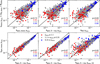 |
Fig. B.1. Comparison of various center shift definitions for the Magneticum galaxy clusters. Coloring indicates whether the galaxy cluster has a formation redshift in the upper (red), middle (gray), or lower third (blue) of the total sample, as given in the legend. |
The top row of Fig. B.1 shows the stellar center shift sstars as a function of the gas mass center shift sgas, m, R200c, the X-ray luminosity sgas, X − ray, R200c, and the total barycenter sall, R200c. We find the agreement between the center shifts to be very tight, with Pearson correlation coefficients in excess of p = 0.7. The stellar center shift apparently best correlated with the total mass center shift, which is likely because the mass is dominated by dark matter that, similar to the stellar particles, is dispersionless. Additionally, we color the points by the galaxy cluster formation redshift, with the upper third of the earliest forming clusters in red, the middle third in gray, and finally those clusters most recently formed in blue (with the formation redshift cuts used given in the legend). The colored values are the Pearson correlation coefficients for their respective third, where we find that the agreement among the different types of center shift is always by far tightest for the most recently formed clusters. We attribute this to the fact that differences in the smaller center shift of a very relaxed, early formed cluster are inherently more spurious.
The second row of Fig. B.1 plots the gas mass center shift sgas, m, R200c versus the X-ray center shift, determined in the same R200c (left, sgas, X − ray, R200c), or within R500c either in three-dimensions (center, sgas, X − ray, R500c) or projected along the z-axis (left, sgas, X − ray, R500c, 2d). We find the gas mass center shift to trace that of the X-ray luminosity remarkably well, even when considering regions farther in or in projection. This is surprisingly true even for the earliest forming clusters (red).
Finally, we also consider differing definitions of where to split the BCG and ICL components used to trace their evolution in Fig. B.2. We show three different definitions for direct comparison. In the left panel, Rcut = 0.1 ⋅ R200c is used as in Fig. 11, which cuts based on the size of the overall halo. The middle panel separates the BCG and the ICL based on the distribution of the central galaxy stars, namely Rcut = 3 ⋅ R*, 1/2, where R*, 1/2 is the radius which contains 50% of the central stellar component within 10%Rvir. This is particularly interesting when comparing to recent observations by Joo & Jee (2023) who report little evolution in the ICL fraction with redshift. They find fICL ≈ 14% already at z > 1, which matches the values we find for the split at Rcut = 3 ⋅ R*, 1/2 at that redshift. This raises the question of whether the radial luminosity profiles at higher redshifts result in a split radius between BCG and ICL that moves increasingly inwards, a process which may be driven by increasingly centrally compact objects at these redshifts (Kimmig et al. 2025; Ito et al. 2024), consequently resulting in a flat evolution in fICL. If instead we split by a fixed aperture, as shown in the right panel of Fig. B.2, we find that at high redshifts practically all of the non-satellite stellar mass in the cluster would be considered part of the BCG. Overall, the fixed aperture and halo based cuts are most similar in terms of the later evolution of galaxy clusters.
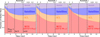 |
Fig. B.2. Same as Fig. 11, but for the Magneticum galaxy clusters using three different definitions of the split between ICL and BCG. Left panel: Same as the left panel of Fig. 11, but with a split between BCG and ICL at 0.1 ⋅ R200, cri. Central panel: BCG and ICL split at 3 ⋅ R*, 1/2, with R*, 1/2 the stellar half mass radius. Right panel: BCG and ICL split at a fixed aperture of 100kpc. |
All Tables
Fit parameters from the orthogonal distance regression for the relations between various parameters for all four simulations.
All Figures
|
Fig. 1. Number of stellar particles equating to the MW-like stellar mass versus the halo mass covered by the simulation. The simulations used for this study are shown in color, with Magneticum Box2 hr shown in blue, TNG100 shown in purple, Horizon-AGN shown in gold, and Hydrangea shown in orange. Other commonly known simulations are shown in gray. Full box cosmological simulations are in light gray, with Mvir, max(z = 0) indicated by a filled circle while the line goes down to the resolution limit of 1000 dark matter particles. Zoom-in simulations are plotted in dark gray, going from the most massive halo in the set (diamond) down to the same 1000 dark matter particle limit (dashed thin line). Vertical dotted lines mark the MW halo mass, the 1014 M⊙ mass threshold used to define clusters, and the Coma cluster mass. Full box simulation suites shown are: Magneticum Pathfinder (Dolag et al. 2025), IllustrisTNG (Nelson et al. 2019b), Horizon-AGN (Dubois et al. 2014), SLOW (Dolag et al. 2023; Seidel et al. 2024), EAGLE (Schaye et al. 2015), Flamingo (Schaye et al. 2023), Millenium-TNG (Pakmor et al. 2023), and Bahamas (McCarthy et al. 2017). Zoom-in simulation suites shown are: Hydrangea (Bahé et al. 2017), Romulus-C (Tremmel et al. 2019), TNG-Clusters (Nelson et al. 2024), Rapsody-G (Hahn et al. 2017), and The300 Project (Cui et al. 2018). |
| In the text | |
|
Fig. 2. Mock images in the r-band of example galaxy clusters from the Magneticum Box2 hr simulation in a random projection, with increasing mass from left to right and cluster IDs indicated in the top left. Clusters in the left column have about M200c = 1 × 10¹⁴ M⊙, with clusters on the right having M200c > 1 × 10¹⁵ M⊙. From top to bottom we plot galaxy clusters with decreasing BCG stellar mass (within 100 kpc, excising satellites) within a narrow bin of cluster halo mass. Each panel shows the full R200c size of the cluster, with the black line in the bottom left of each panel marking the effective length of 100 kpc while the axes ticks are in units of 0.2r200c. |
| In the text | |
|
Fig. 3. Left: Stellar mass of the central BCG within 100 kpc versus the total halo mass M200c for the four simulations, scaled to a common h. Magneticum is plotted in blue, IllustrisTNG in purple, Hydrangea in orange and Horizon-AGN in gold. Center: Same stellar mass plotted against the halo mass as given by M500c. Also plotted are observations by DeMaio et al. (2018) and Kravtsov et al. (2018). Right: Total stellar mass (BCG, ICL and satellites) against M500c for the simulations, as well as observations by Andreon (2012), Laganá et al. (2013), Gonzalez et al. (2013), Budzynski et al. (2014), Kravtsov et al. (2018), Sartoris et al. (2020). |
| In the text | |
|
Fig. 4. Histograms of the formation redshifts for all clusters from Magneticum Box2 hr (blue), Hydrangea (orange), Horizon-AGN (gold), and TNG100 (purple), going from top to bottom. Median (solid) and 1-σ bounds (dashed) are indicated as vertical lines. |
| In the text | |
|
Fig. 5. Upper row: Evolution of the halo mass M200, c with redshift z for all clusters in the Magneticum Box2 hr simulation, normalized to the final mass M200, c(z = 0). The black line shows the median, with the dark shaded area marking the 1σ-bounds and the light shaded area marking the 2σ-bounds. The colored lines and their 1σ-bounds show the evolution of a subset of clusters split by their formation redshift (left) or their fICL + BCG (right) as given in the legend. Black dash-dotted vertical lines mark the redshifts at which the average cluster has accumulated 20%, 50%, and 90% of its total mass (horizontal black lines), marked by z20, z50, and z90, respectively. We note that z50 is what we define as formation redshift of a cluster. Lower row: Evolution of fICL + BCG with redshift z. As in the upper panel, the black line marks the average evolution of all clusters from Magneticum, with the gray shaded areas showing the 1σ- and 2σ-bounds. The colored lines and regions show the median and 1σ-bounds for the same subsets of galaxy clusters. |
| In the text | |
|
Fig. 6. Left panel: Fraction of stellar mass within R200c that is not bound to satellites but instead in the BCG or ICL, fICL + BCG, against the halo mass M200c, for the Magneticum (blue), IllustrisTNG (purple), Horizon-AGN (gold) and Hydrangea (orange) clusters. Right panel: Same as the left panel but for the Magneticum galaxy clusters only, colored by the cluster formation redshift zform. Colors as indicated in the legend. |
| In the text | |
|
Fig. 7. Upper panel:fICL + BCG versus formation redshift zform, for the galaxy clusters from the Magneticum (blue), TNG100 (purple), Horizon-AGN (gold), and Hydrangea simulations (orange). The gray box displays the Pearson correlation coefficient for each simulation between fICL + BCG and zform. The closer the absolute value is to unity, the tighter the correlation. We further include best fit lines for each simulation determined via the least squares method (colored lines). Middle panel: Center shift between the 3D gas barycenter and the location of the BCG (normalized by R200c), plotted as a function of the formation redshift, with the colors the same as the upper panel. Lower panel: Fraction of the total halo mass mass which is in all subhalos fsub (so excluding the central and diffuse halo) versus formation redshift, with colors as in the upper two panels. |
| In the text | |
|
Fig. 8. Comparison of fICL + BCG against different dynamical tracers for all individual clusters from Magneticum Box2 (blue), TNG100 (purple), Horizon-AGN (gold), and Hydrangea (orange). The numbers in each panel indicate the Pearson correlation coefficient found for each relation and simulation (colors). We plot fICL + BCG against the stellar mass ratio of the BCG to the second (left panel) and fourth (second panel) most massive galaxy inside the cluster, counting the BCG. The third panel shows fICL + BCG as a function of the offset between the stellar barycenter and the BCG position sstars, while the right panel plots the fraction against the stellar potential ϕstars = M*/R*, half determined within 0.1 ⋅ R200c. |
| In the text | |
|
Fig. 9. Full matrix of the correlation strength between different parameters, with darker colors indicating stronger correlations, for all four simulations as indicated at the respective tiles for each panel. From top to bottom and left to right are the same parameters, in the following order: formation redshift zform, the fraction of stellar mass within ICL plus BCG fICL + BCG, the center shift between the stellar (sstars) or gas barycenter (sgas) and the BCG, the fraction of total mass within all substructures fsub or within just the 8th most massive substructure f8, the stellar mass ratio between the BCG and the second (M12) or fourth (M14) most massive galaxy in a cluster, the central stellar potential ϕBCG, the passive fraction fquench of galaxies in the cluster with stellar masses above 1 × 10¹⁰ M⊙ as well as their total number Nsat, and the total halo mass M200c. We note that black squares in the diagonal mark the self-correlation of the parameters and are thus all equal to one. |
| In the text | |
|
Fig. 10. Stellar mass-halo mass relation for the Magneticum Box2 hr clusters. The gray points show the total stellar mass within R200c, including the BCG, ICL and satellites. The colored symbols show the stellar mass of only the ICL and the BCG together, without including satellite galaxies. These points are colored according to the formation redshift of the cluster from older and more relaxed galaxy clusters (red) to younger, recently assembled clusters (blue). |
| In the text | |
|
Fig. 11. Fraction of the total stellar mass contained in the different components of the Magneticum Box2 hr galaxy clusters versus time, determined for all clusters (left panel) and for the 50 clusters with the highest (central panel) and the 50 clusters with the lowest fICL + BCG for their halo mass (right panel). The fraction of stellar mass contained within the BCG is shown in red, while the fraction in the ICL, the second most massive satellite, and all other satellites are plotted in gold, violet and blue, respectively. The black vertical lines mark the times when the median mass of each group of galaxy clusters is M200, cri > 1 × 10¹³ M⊙ (dotted), M200, cri > 5 × 10¹³ M⊙ (dashed), and M200, cri > 1 × 10¹⁴ M⊙ (dash-dotted). We note that here we split the BCG and ICL at 0.1 × R200, cri. For different definitions of the split between the ICL and the BCG, see Fig. B.2 in the Appendix. |
| In the text | |
|
Fig. 12. Absolute change in fICL + BCG versus the relative change in mass δM200c as determined over a period of T = 1 Gyr for the Magneticum clusters. Columns from left to right split the sample into redshift bins, while the rows separate the clusters based on their current mass, going from all clusters in the top row to small and massive groups and finally clusters on the bottom row. The median line and 1σ-bounds are plotted in black, while the thin vertical and horizontal black lines show the location of zero change in either fICL + BCG or cluster mass. y0 indicated in each panel is the median change in fICL + BCG for halos where the total mass did not change, δM200c = 0. |
| In the text | |
|
Fig. A.1. Partial correlation of zform with fICL + BCG, accounting for other parameters X (blue), or between zform and X, accounting for fICL + BCG (red), for all four simulations (panels). |
| In the text | |
|
Fig. A.2. Top row: The Magneticum data as in Fig. 7, with the axes swapped. Solid lines show the best fits using either the least-squares method, fitting toward x (red) or y (blue), as well as the best fit using orthogonal distance regression (black). Bottom row: Cumulative histogram of the absolute offset between the predicted versus actual formation redshifts for the three best fit lines, as well as when drawing randomly from a normal distribution of formation redshifts with the mean and standard deviation calculated from the total sample of clusters (gray). The 1σ-bounds (68.27%) are shown as colored vertical lines. |
| In the text | |
|
Fig. B.1. Comparison of various center shift definitions for the Magneticum galaxy clusters. Coloring indicates whether the galaxy cluster has a formation redshift in the upper (red), middle (gray), or lower third (blue) of the total sample, as given in the legend. |
| In the text | |
|
Fig. B.2. Same as Fig. 11, but for the Magneticum galaxy clusters using three different definitions of the split between ICL and BCG. Left panel: Same as the left panel of Fig. 11, but with a split between BCG and ICL at 0.1 ⋅ R200, cri. Central panel: BCG and ICL split at 3 ⋅ R*, 1/2, with R*, 1/2 the stellar half mass radius. Right panel: BCG and ICL split at a fixed aperture of 100kpc. |
| In the text | |
Current usage metrics show cumulative count of Article Views (full-text article views including HTML views, PDF and ePub downloads, according to the available data) and Abstracts Views on Vision4Press platform.
Data correspond to usage on the plateform after 2015. The current usage metrics is available 48-96 hours after online publication and is updated daily on week days.
Initial download of the metrics may take a while.