| Issue |
A&A
Volume 700, August 2025
|
|
|---|---|---|
| Article Number | A211 | |
| Number of page(s) | 25 | |
| Section | Extragalactic astronomy | |
| DOI | https://doi.org/10.1051/0004-6361/202554970 | |
| Published online | 26 August 2025 | |
Constraining the [C II] luminosity function from the power spectrum of line-intensity maps at redshift 3.6
1
Argelander-Institut für Astronomie, Universität Bonn, Auf dem Hügel 71, 53121 Bonn, Germany
2
SISSA, International School for Advanced Studies, Via Bonomea 265, 34136 Trieste, Italy
3
Dipartimento di Fisica – Sezione di Astronomia, Università di Trieste, Via Tiepolo 11, 34131 Trieste, Italy
4
IFPU, Institute for Fundamental Physics of the Universe, Via Beirut 2, 34151 Trieste, Italy
⋆ Corresponding author: This email address is being protected from spambots. You need JavaScript enabled to view it.
Received:
1
April
2025
Accepted:
6
July
2025
Abstract
Context. Forthcoming measurements of the line-intensity mapping (LIM) power spectrum (PS) are expected to provide valuable constraints on several quantities of astrophysical and cosmological interest.
Aims. We focus on the [C II] luminosity function (LF) at high redshift, which remains poorly constrained, especially at the faint end. As an example of future opportunities, we present forecasts for the Deep Spectroscopic Survey (DSS) that is to be conducted with the Fred Young Submillimeter Telescope (FYST) at z ≃ 3.6. We also make predictions for hypothetical surveys with a ten times larger sky coverage and/or a sensitivity that is higher by a factor of √10. We account for the Lorentzian spectral profile of Fabry-Pérot interferometers and investigate the effect of their increased resolving power R on the constraints.
Methods. Motivated by the halo-occupation properties of [C II] emitters in the MARIGOLD simulations, we used an abundance-matching approach to connect two versions of the ALPINE LF to the halo mass function. The resulting luminosity–mass relation was used in a halo-model framework to predict the PS signal and its uncertainty. Bayesian inference on mock PS data allowed us to forecast constraints on the first two LF moments and Schechter function parameters.
Results. Depending on the true LF, the DSS is expected to be able to detect clustering and shot-noise components with signal-to-noise ratios of ≳2. At R = 100, spectral smoothing overwhelms the signal from redshift-space distortions, rendering the associated damping scale σ unmeasurable. For R ≳ 500, σ can be distinguished from instrumental effects, although the degeneracies with amplitude parameters increase. Joint fits to the PS and LF yield precise constraints on the Schechter normalisation and cutoff luminosity, while the faint-end slope remains uncertain (unless the true value approaches −2).
Conclusions. An increased survey sensitivity offers greater gains than a wider area. A higher spectral resolution improves the access to physical parameters, but intensifies degeneracies. This highlights key design trade-offs in LIM surveys.
Key words: methods: statistical / galaxies: high-redshift / galaxies: luminosity function / mass function / large-scale structure of Universe
© The Authors 2025
 Open Access article, published by EDP Sciences, under the terms of the Creative Commons Attribution License (https://creativecommons.org/licenses/by/4.0), which permits unrestricted use, distribution, and reproduction in any medium, provided the original work is properly cited.
This article is published in open access under the Subscribe to Open model. This email address is being protected from spambots. You need JavaScript enabled to view it. to support open access publication.
1. Introduction
Line-intensity mapping (LIM) is an emerging observational technique that takes advantage of modern imaging cameras that operate at wavelengths from the far-infrared to the radio regime (see Kovetz et al. 2017; Bernal & Kovetz 2022, for recent reviews). It aims to map fluctuations in the intensity of redshifted radiation that is emitted in specific spectral lines over large areas of the sky without resolving individual sources. The output consists of a data cube in which the radiation intensity is recorded as a function of the sky position and frequency. By assuming a cosmological model, this data cube can be transformed into a three-dimensional map of the line intensity, where the size of each voxel is determined by the angular and spectral resolution of the observations. LIM records the cumulative signal from all sources, including the contribution from the faintest galaxies that are missed in traditional flux-limited surveys.
Line-intensity mapping was first proposed for studying the epoch of cosmic reionisation through the 21 cm hyperfine line of atomic hydrogen (Hogan & Rees 1979; Scott & Rees 1990; Madau et al. 1997; Furlanetto et al. 2006) in emission or absorption against the cosmic microwave background (CMB). It was later realised that the 21 cm emission from the post-reionisation Universe might be used as a cosmological probe: Except for a multiplicative normalisation factor and an additive shot-noise term, the power spectrum (PS) of the signal from the neutral hydrogen that is locked up in galaxies and damped Lyman-α systems matches the matter PS on large scales, and it thus encodes cosmological information (Wyithe & Loeb 2007; Chang et al. 2008). At the same time, the normalisation and shot-noise terms can be used to constrain the luminosity function (LF) of theemitters.
In addition to the 21 cm transition, LIM has been proposed to be applied to other spectral lines by targeting different regions of the electromagnetic spectrum. For instance, it was suggested to employ this technique in the millimetre and centimetre bands in order to detect the cumulative emission from the first galaxies (at redshift z > 10) through the brightest atomic gas-cooling lines (Suginohara et al. 1999). Righi et al. (2008) estimated the contribution to CMB foregrounds that is generated by redshifted rotational transitions of the CO molecule and the [C II] fine-structure line from singly ionised carbon and concluded that LIM experiments would play a key role in reducing theoreticaluncertainties.
Later, CO transitions, [C II] and, more recently, [O III] were suggested as possible tracers of the large-scale structure (LSS) of the Universe at high redshift (e.g. Visbal & Loeb 2010; Carilli 2011; Lidz et al. 2011; Gong et al. 2012; Pullen et al. 2013, 2018; Breysse et al. 2014; Dumitru et al. 2019; Padmanabhan 2019; Padmanabhan et al. 2022). Similarly, the redshifted Lyα line of atomic hydrogen was considered for LIM experiments in the near-infrared (Silva et al. 2013; Pullen et al. 2014).
In the past decade, there has been an ever-increasing activity in proposing applications of LIM to miscellaneous topics in astrophysics (e.g. Lidz et al. 2009; Gong et al. 2012; Visbal et al. 2015; Comaschi & Ferrara 2016; Breysse & Rahman 2017) and cosmology (e.g. Karkare & Bird 2018; Bernal et al. 2019, 2021; Moradinezhad Dizgah & Keating 2019; Muñoz et al. 2020; Bauer et al. 2021; Moradinezhad Dizgah et al. 2022). This fervid forecasting endeavour provided the basis for developing about 30 dedicated instruments1 for LIM from the ground, balloon based, and from space.
Unlocking the full potential of LIM experiments requires a careful characterisation and mitigation of systematic effects that contaminate the measurements. These include foregrounds and backgrounds with continuous spectra (due to radio-frequency interference, the atmosphere, the Galaxy, the cosmic infrared background, and the CMB, depending on the wavelength) as well as spectral line interlopers (i.e. line emission from different transitions that is redshifted at the same observed frequencies). Developing efficient foreground-cleaning techniques is a very active research field, and numerous different methods were proposed (e.g. Breysse et al. 2015; Silva et al. 2015; Sun et al. 2018). Detections of the LIM signal were originally achieved through cross-correlations with galaxy surveys for the 21 cm line (e.g. Masui et al. 2013; Anderson et al. 2018; CHIME Collaboration 2022; Wolz et al. 2022) and [C II] Pullen et al. (2018). Recently, a direct detection of the H I PS at 0.32 < z < 0.44 (Paul et al. 2023) and tentative detections of the shot-noise PS from rotational CO lines (Keating et al. 2016, 2020; Ihle et al. 2022; Stutzer et al. 2024) have been obtained.
In this work, we explore the potential of the LIM PS to constrain the [C II] LF at redshift z > 3.5, when the Universe was younger than 1.8 Gyr. With the advent of new observational facilities such as the Atacama Large Millimeter/sub-millimeter Array (ALMA) and the Northern Extended Millimeter Array (NOEMA), it is now possible to routinely detect [C II] line emission from individual high-redshift galaxies, and thus, to probe the physical conditions of their interstellar medium. It is, however, extremely challenging to conduct wide surveys and collect samples that are statistically representative of the underlying population (see Sect. 3.1 for further details). Hence, the [C II] LF at such early times still remains very poorly constrained, particularly at the faint end. Knowledge of this quantity, however, would likely allow us to determine the evolution of the cosmic star formation rate density in a way that is unaffected by dust obscuration. In addition, it would provide a stringent test of galaxy-formation models that are able to predict [C II] emission (e.g., among others, Vallini et al. 2015; Popping et al. 2016; Olsen et al. 2017; Lagache et al. 2018; Lupi et al. 2018; Leung et al. 2020; Khatri et al. 2025).
As an example of the forthcoming capabilities that will enable the detection of the [C II] LIM signal, we use the specifics of the Deep Spectroscopic Survey (DSS) as a reference setup. This survey will be conducted with the 6-meter Fred Young Submillimeter Telescope (FYST), which is located near the top of Cerro Chajnantor at an elevation of 5600 m in the Atacama desert (CCAT-Prime Collaboration 2023). We also consider the impact of larger sky coverages and/or higher sensitivities. Moreover, we investigate the effect of changes in the spectral resolving power on the measurement of parameters related to redshift-space distortions. In all cases, we focus on a narrow redshift interval centred around z ≃ 3.6.
The paper is organised as follows. In Sect. 2 we outline the halo model for the LIM PS. The current state of measurements of the [C II] LF at high redshift is summarised in Sect. 3, where we also present the analysis of the MARIGOLD simulations and introduce the abundance-matching technique. In Sect. 4 we present our predictions for the LIM PS and its uncertainty. In Sect. 5 we describe our Bayesian-inference pipeline and present the results we obtained from the analysis of mock data. In Sect. 6 we finally summarise our findings.
We adopt a flat Friedmann-Lemaître-Robertson-Walker cosmological background with dimensionless Hubble constant h = 0.674 and present-day density parameters Ωm = 0.315, Ωb = 0.049, and ΩΛ = 0.685 for matter, baryons, and the cosmological constant, respectively. The PS of primordial density perturbations is characterised by the spectral index ns = 0.965 and the normalisation factor σ8 = 0.811. We compute the linear PS in the standard ΛCDM scenario with the Code for Anisotropies in the Microwave Background (CAMB2, Lewis et al. 2000).
2. Halo model for LIM
In the absence of absorption and scattering (and neglecting redshift corrections due to peculiar velocities), the specific intensity of radiation detected at frequency νo along the line of sight  by an observer at redshift zero is
![Mathematical equation: $$ \begin{aligned} I_\nu (\nu _{\rm o},\mathbf n )=\frac{1}{4\pi } \int _0^\infty \epsilon _\nu [(1+z)\,\nu _{\rm o},\hat{\mathbf{n }},z]\,\frac{1}{1+z}\,\frac{{\mathrm{d} } \chi }{{\mathrm{d} } z}\,{\mathrm{d} } z, \end{aligned} $$](/articles/aa/full_html/2025/08/aa54970-25/aa54970-25-eq3.gif) (1)
(1)
where  is the comoving-volume emissivity at rest-frame frequency νe due to sources at redshift z and
 (2)
(2)
denotes the comoving radial distance per unit redshift, with H the Hubble parameter. Considering line emission with a frequency spectrum that can be approximated with a Dirac delta function, we can write
 (3)
(3)
where ρL denotes the total luminosity emitted per unit comoving volume and νrf is the rest-frame central frequency of the transition. Replacing this expression in Eq. (1) gives
 (4)
(4)
which shows that the signal observed at frequency νo is fully generated at redshift z* = νrf/νo − 1. This signal is difficult to isolate from observations because of the presence of much more luminous foregrounds with continuum spectra and various interloper lines. Dedicated techniques are being developed to separate the signal from the spectrally smooth foregrounds and mitigate the impact of the interlopers (e.g. Alonso et al. 2015; Li et al. 2019; Karoumpis et al. 2024; Roy & Battaglia 2024; Bernal & Baleato Lizancos 2025).
2.1. Mean signal
The mean specific intensity over the sky is
 (5)
(5)
where the mean comoving luminosity density  coincides with the first moment of the LF of line emitters at fixed redshift,
 (6)
(6)
With a little abuse of notation, in the remainder of this paper, we will write  to indicate
  with νo = νrf/(1 + z).
2.2. Power spectrum
The spatial fluctuations around the mean signal, that is,  , encode precious astrophysical and cosmological information. By adopting a fiducial cosmological model, it is possible to convert the pair of observables
  into the position vector
  and thus build a three-dimensional map of δIν on the past light cone of the observer. The information content of the map is then compressed into clustering summary statistics such as the PS.
Assuming that line emission takes place only within dark-matter (DM) haloes provides a particularly convenient framework to model the statistical properties of δIν. The key ingredient is the conditional luminosity function (CLF), ϕ(L|M, z), which gives the differential distribution of the number of galaxies hosted, on average, within haloes of mass M and redshift z, as a function of their line luminosity. By definition,
 (7)
(7)
where  denotes the halo mass function, i.e. the mean number density of haloes per unit mass. For later use, we introduce the moments of the CLF
 (8)
(8)
with n ∈ ℕ. η0 gives the mean number of emitters hosted by a DM halo of mass M at redshift z, η1 gives the mean total luminosity emitted within the halo, and η2 gives the mean sum of the squared luminosities of the individual emitters. Obviously,
 (9)
(9)
which decomposes the mean comoving emissivity into the contribution from different halo masses.
As commonly done in the literature (e.g. Lidz et al. 2011), we computed the large-scale PS of the specific intensity by assuming that: (i) DM haloes are linearly biased with respect to the underlying matter distribution (i.e. their overdensity δh = bh δ with bh a function of M and redshift), (ii) the scales of interest are significantly larger than the virial radii of the relevant haloes, (iii) the surveyed patch of the sky has a small extension compared to the distance to the observer so that we can assume a fixed line-of-sight direction  (distant-observer approximation), (iv) there is no peculiar-velocity bias, and (v) fluctuations of the CLF and halo counts are Poissonian. It follows from these assumptions that the redshift-space PS of the specific intensity receives two contributions
 (10)
(10)
with Pclust arising from the clustering of the line-emitting galaxies and Pshot originating from the fact that they are discrete objects and thus show random fluctuations in their number counts within a finite volume. Given that the clustering signal only dominates on large scales and that the measurements we consider have relatively large uncertainties, it is sufficient to use linear perturbation theory to model the different components.
The clustering component can be expressed in terms of the linear matter PS, Pm, as
![Mathematical equation: $$ \begin{aligned} P_{\rm clust}(k,\mu ,z)=\bar{I}_\nu ^2(z)\,[b(z)+f(z)\, \mu ^2]^2\,\mathcal{D} (k,\mu ,z)\,P_{\rm m}(k,z), \end{aligned} $$](/articles/aa/full_html/2025/08/aa54970-25/aa54970-25-eq22.gif) (11)
(11)
where the linear bias coefficient
 (12)
(12)
f is the growth-rate of structure, and  .
.
The term 𝒟 in Eq. (11) is a phenomenological damping factor accounting for the non-perturbative suppression of clustering in redshift space due to velocity dispersion of the line-emitting regions within their host haloes. This approximation has been first introduced to model galaxy clustering in redshift space (e.g. Peacock & Dodds 1994). The three most common choices in the literature for the damping function are Gaussian, Lorentzian, and squared Lorentzian shapes:
![Mathematical equation: $$ \begin{aligned} \mathcal{D} (k,\mu ) = {\left\{ \begin{array}{ll} \exp (-k^2\mu ^2\sigma ^2),\\ \left[1+(k\mu \sigma )^2\right]^{-1},\\ \left[1+\displaystyle {\frac{(k\mu \sigma )^2}{2}}\right]^{-2}, \end{array}\right.} \end{aligned} $$](/articles/aa/full_html/2025/08/aa54970-25/aa54970-25-eq25.gif) (13)
(13)
which all behave as 1 − k2μ2σ2 when k → 0. Here, the parameter σ denotes a typical comoving displacement which should agree, within a factor of order unity, with the pairwise velocity dispersion divided by aH. In this work, we used a squared Lorentzian damping function but our conclusions do not change if another of the shapes presented in Eq. (13) is adopted.
The shot-noise component does not depend on k and assumes the redshift-dependent value of
 (14)
(14)
where the ‘effective number density’ of emitters satisfies
 (15)
(15)
which can also be expressed as (Cheng et al. 2019)
 (16)
(16)
3. [C II] emission
The C+ ion is the most abundant form of carbon under many astrophysical conditions. In particular, since the first and second ionisation potentials of carbon (11.26 and 24.38 eV, respectively) bracket the hydrogen ionisation potential (13.6 eV), C+ is present also in regions where hydrogen is neutral.
The ground electronic state of C+ has two fine structure levels separated by approximately 0.0079 eV (corresponding to a temperature of 91.25 K). The associated 2P3/2−2P1/2 magnetic-dipole transition (hereafter [C II]) at 157.74 μm (1900.5369 GHz) is one of the main coolants of the neutral and ionised interstellar medium (ISM). Thanks to its long wavelength, [C II] radiation can traverse gas and dust with very little attenuation.
Due to telluric water-vapour absorption, [C II] emission from the local Universe can only be detected with far-infrared balloon-, aircraft- or space-based observatories. For cosmological sources with 3.3 < z < 9.3, however, the (redshifted) [C II] line becomes accessible from the ground (at special high-altitude sites) when it falls in one of the sub-millimetre or millimetre atmospheric windows.
Recent interferometers such as ALMA and NOEMA allow us to observe [C II] at high angular (and spectral) resolution and thus probe the physical conditions of gas in these high-redshift galaxies.
Local and cosmological observations reveal that [C II] is one of the brightest emission lines from star-forming galaxies which typically accounts for 0.01% to 1% of the total far-infrared (FIR) luminosity (e.g. Stacey et al. 2010). The precise source of the emission remains unclear as the line can, in principle, arise from a variety of phases of the interstellar medium including molecular, atomic, and ionised gas. Depending on the detailed physical conditions of the gas, the line can be easily excited by collisions with electrons, hydrogen atoms, and hydrogen molecules. At high redshift, the CMB provides a background of continuum radiation (the CMB spectrum peaks at the [C II] central wavelength for z ≃ 5.6) which leads to an attenuation of [C II] emission from low density gas (Goldsmith et al. 2012).
It is widely believed that, at high redshift, [C II] should predominantly originate from photon-dominated regions at the boundaries of molecular clouds which are exposed to the ionising flux of nearby young stars (Stacey et al. 2010; Pineda et al. 2014; Gullberg et al. 2015; Vallini et al. 2015; Lagache et al. 2018).
In local, normal, star-forming galaxies, the [C II] luminosity correlates with the star formation rate (and metallicity) although with a larger scatter compared with other lines (e.g. De Looze et al. 2014). A widespread explanation for this correlation invokes energy balance: namely, in thermal equilibrium, the heating and cooling rates of the gas in the neutral atomic phase of the ISM must match. The correlation arises from the fact that [C II] is the dominant cooling line while the main heating source is collisions with photoelectrons ejected by dust grains and polycyclic aromatic hydrocarbon molecules due to ultraviolet radiation emitted by young massive stars. Observations also showed, however, that the [C II]/FIR luminosity ratio decreases with increasing infrared luminosity (Malhotra 2001), which is expected to be an accurate star-formation tracer as it originates from UV and optical emission from young stars absorbed and re-radiated by dust at longer wavelengths. This so-called ‘[C II] deficit’ is not fully understood yet and casts doubts on the use of [C II] as a general star-formation tracer. Similar correlations (with different normalisations) and trends are seen in high-redshift galaxies (e.g. Carniani et al. 2018; Schaerer et al. 2020).
3.1. [C II] luminosity function
The unprecedented sensitivity of ALMA to [C II] emission makes it an ideal tool to conduct follow-up observations of pre-selected galaxies at high redshift. Because its field of view is small, however, it is very time consuming to carry out untargeted surveys that cover large fractions of the sky. Only a few blind surveys were therefore conducted so far. The ALMA Large Program to INvestigate CII at Early Times (ALPINE, Le Fèvre et al. 2020; Béthermin et al. 2020; Faisst et al. 2020) invested 70 hours of observations in band 7 (275−373 GHz) to perform targeted observations of 118 main-sequence galaxies (selected by their rest-frame UV luminosity at 1500 Å with an absolute-magnitude limit of M1500 < −20.2) in the redshift range 4.4 < z < 5.9 (excluding the range 4.6 < z < 5.12 for which the [CII] line falls in a low transmission window for ALMA). It also conducted a blind search within the 118 pointings (covering 24.92 arcmin2 in total) which detected eight secure and four likely [C II] emitters. Eleven of the twelve sources are strongly clustered around the central target in the same pointing. Loiacono et al. (2021, hereafter L21) used these emitters to estimate the [C II] LF in the ‘cluster’ environment. They parametrised their results in terms of the Schechter function
 (17)
(17)
or, equivalently,
 (18)
(18)
where Φ* and Ψ* = ln10 Φ* are normalisation factors, L* is the characteristic luminosity at which the counts are exponentially suppressed, and α is the slope of the power law describing the low-luminosity regime (without a cutoff at low L, the galaxy number density diverges if α ≤ −1 but the luminosity density only diverges if α ≤ −2). It turns out that the data poorly constrain L* and an informative prior (L* < 1010.5 L⊙) was used. The best-fit parameters are reported in Table 1. We note that α is poorly constrained given the lack of information at faint luminosities. Based on the ratio between the number of unclustered and clustered sources, L21 estimated that the ‘field’ LF should be a factor of ∼11 lower than the ‘cluster’ one (assuming that the shape is the same).
Another estimate of (and Schechter fit to) the [C II] LF in the same redshift range has been presented by Yan et al. (2020, hereafter Y20). This was obtained by combining the serendipitous and targeted [C II] ALPINE detections with additional data in the far-IR continuum and for CO line emission (Koprowski et al. 2017; Decarli et al. 2019; Riechers et al. 2019; Gruppioni et al. 2020) that were converted into [C II] luminosities using empirical scaling relations. The best-fit parameters are presented in Table 1 together with their relatively large uncertainties. The LF is in agreement with (but slightly lower than) the results by L21 for the cluster sample (see Fig. 1).
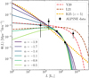 |
Fig. 1. [C II] LF estimated from the targeted ALPINE detections by Yan et al. (2020, Y20) (black data points and error bars). We show the average between the estimates at redshift z ∼ 4.5 and 5.5. Our Schechter fits to the data are superposed with different fixed values of the faint-end slope α (purple, blue, and green lines). The dashed red line shows the LF fit obtained by Y20 combining multiple datasets at different wavelengths. The fit by Loiacono et al. (2021, L21) to the serendipitous (and clustered) ALPINE detections is shown with a dashed brown line. For comparison, the LF from the MARIGOLD numerical simulations by Khatri et al. (2025, K25) at z = 5 is represented by a dotted gold line. |
Schechter fits to the observed [C II] LF from L21 and Y20.
The targeted ALPINE detections possibly miss UV-faint but [C II]-bright galaxies. They can therefore only provide a lower limit to the total LF. On the other hand, the serendipitous detections are scarce and their LF carries large statistical uncertainties. Moreover, they are affected by clustering which leads to a systematic overestimation of the LF. Given this state of the art, in the remainder of this paper, we follow a twofold strategy. Namely, we use the fit by Y20 as an upper limit to the LF which we refer to as the optimistic case. Moreover, as a lower limit, we produce our own least-squares fits to the LF of the targeted detections by considering different fixed values of α (see Fig. 1) which we refer to as the pessimistic case.
3.2. [C II] emitters in the MARIGOLD simulations
In order to develop insights about the halo-occupation properties of [C II] emitters, we use the MARIGOLD simulations presented in Khatri et al. (2025). MARIGOLD are a suite of cosmological simulations of galaxy formation which account for gravity, adaptive-mesh-refinement fluid dynamics, star formation, stellar feedback, the propagation of the ionising radiation emitted from young stars, and include the HYACINTH module for interstellar chemistry (Khatri et al. 2024). Given the computational cost of such an effort, the simulations follow the formation of structure until z = 3 within periodic cubic boxes of different comoving side lengths L and achieve different spatial resolutions Δx. The high-resolution simulation has L = 25 Mpc and a minimum grid size of Δx = 32 pc. The low-resolution simulation, instead, has L = 50 Mpc and Δx = 64 pc. [C II] emission is computed in post processing by solving the radiative transfer equation (i.e. without assuming the line is optically thin) as detailed in Khatri et al. (2025). This calculation can be robustly performed for haloes and subhaloes with M ≥ 109 h−1 M⊙.
Fig. 2 shows a synthetic image of the [C II] emitters hosted within a massive DM halo at z = 5. The central galaxy is the dominant source and is surrounded by more than a dozen substantially fainter emitters. This is a typical situation as evidenced in Fig. 3 where we plot the conditional luminosity function extracted from the simulations in three different mass bins. We distinguish between central and satellite [C II] emitters. The central ones encompass the region within 0.1 virial radii from the stellar centre of mass of the main galaxy. Satellites extend up to the tidal radius of the subhaloes. In the most massive bin we consider, 1011 ≤ M/(h−1 M⊙) < 1012 (bottom panel3), the central galaxies present a narrow distribution of luminosities (with a median value of log10L/L⊙ = 7.84 and a logarithmic width of 0.51, see Table 2) which overlaps with the range covered by the ALPINE detections. Each halo contains, on average, 5.58 satellites which follow a very broad distribution of luminosities with a median value of log10L/L⊙ = 5.93. Their aggregated luminosity only accounts for 28% of the total [C II]emission (see Table 2). The integrated contribution from satellites becomes even less important for lower mass bins (top two panels). The results related to these halo masses are influenced by the finite mass resolution of the simulation. For this reason, we examined the contribution of centrals and satellites in the mass bins spanning from 109 to 1011 h−1 M⊙ using the high-resolution MARIGOLD simulation.
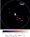 |
Fig. 2. Surface brightness of the [C II] emitters hosted by a DM halo of mass M = 5.78 × 10¹¹ h−1 M⊙ in the z = 5 snapshot of the low-resolution MARIGOLD simulation. The circle indicates the virial radius ofthe halo. |
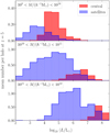 |
Fig. 3. CLF extracted from the MARIGOLD simulations at z = 5 in three halo mass bins. The contributions from central and satellite [C II] emitters are indicated in different colours. The scale of the y-axis changes in the different panels. Quantitative information about the CLF is provided in Table 2. The top two panels refer to the high-resolution simulation, and the bottom panel is obtained from the low-resolution simulation, which contains more massive haloes. |
We note that the median luminosity of the central galaxies scales approximately as Mγ with 1.2 < γ < 1.5 while satellites show a much shallower slope of 0.2 < γ < 0.7. It turns out that, for every [C II] luminosity we can probe, at least 80% of the emitters are central galaxies and this fraction reaches 100% for the brightest ones.
3.3. Abundance matching
We now return to discussing about the actual [C II] emitters. Based on the simulation results presented above, in the remainder of this paper, we assume that each halo contains only one source and that there is no scatter in the [C II] luminosity at fixed mass, i.e. ϕ(L|M) = δD[L − ℒ(M)], which, once inserted in Eq. (8), gives ηn(M, z) = [ℒ(M)]n. Further assuming that ℒ(M) is a monotonic function (always growing with M) allows us to determine its inverse function by a simple abundance-matching procedure. In fact, by integrating Eq. (7) in L, we obtain
 (19)
(19)
For instance, this approach has been used in Padmanabhan (2018) to model LIM of the CO line (see also Padmanabhan 2019, 2023; Padmanabhan et al. 2022).
We evaluated the halo mass function  using the fit to numerical simulations by Sheth et al. (2001) but setting their parameter q = 1 as in Schneider et al. (2013). This requires calculating the variance of the smoothed linear density perturbations, for which we adopted the so-called ‘smooth-k’ window function 1/[1 + (kR)β] (Leo et al. 2018) with β = 4.8. For the smoothing radius, we used R = RTH/3.3, where RTH denotes the comoving Lagrangian radius of a spherical perturbation of mass M. These choices provide an excellent fit to N-body simulations in different cosmological scenarios (Sameie et al. 2019; Bohr et al. 2021; Parimbelli et al. 2021) and allow us to extend our calculations beyond CDM in our future work (Marcuzzo et al., in prep.).
Results based on the halo mass function at redshift z = 5 (chosen as representative of the ALPINE redshift range) are displayed in Fig. 4. At the low-mass end, the halo mass function follows a power-law behaviour with a slope close to −2. If the faint-end slope of the luminosity function satisfies α > −1, then the total number density of [C II]-emitting galaxies converges to a finite value. In this case, the abundance-matching procedure imposes a sharp lower cutoff in the luminosity–mass relation ℒ(M) at the halo mass corresponding to that number density (≃1011 h−1 M⊙ for the case shown in the figure). In contrast, when −2 < α ≤ −1, the cumulative number density of emitters increases more slowly with decreasing luminosity than the halo number density increases with decreasing mass. As a result, the corresponding relation between luminosity and halo mass, η1(M) = ⟨L|M⟩, exhibits a smoother transition at low masses rather than an abrupt cutoff. This transition occurs around M ≲ 1011 h−1 M⊙, where the halo mass function approximates a power law. The steepness of the transition depends on α and approximately scales as M−1/(1 + α) in the low-mass regime. Finally, we point out that our result for α = −1.7 shows excellent agreement with the η1(M, z) relations extracted from the MARIGOLD simulations at z = 5 and z = 4 (shown by the dotted gold and dark gold lines in Fig. 4).
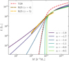 |
Fig. 4. [C II] luminosity as a function of halo mass obtained via abundance matching. The colours for the solid-line fits to the ALPINE data at z ≃ 5 are the same as in Fig. 1. The dashed red line refers to the LF fit obtained by Y20. The dotted gold and dark gold lines show the actual η1 function (i.e. the mean total luminosity per halo) extracted by K25 at z = 5 and z = 4, respectively. |
In Fig. 5, we use the simulations to directly test how accurate is the function ℒ(M) determined via abundance matching. The blue hexagons in the scatter plot show the total [C II] luminosity vs. halo mass. The total luminosity is obtained by summing up the contributions of all the resolved emitters hosted within a single halo. The black symbols indicate the mean (total) luminosity within narrow logarithmic mass bins and thus provide an estimate of the function η1(M, z = 5). The result is monotonically increasing with M as we assumed in Sect. 3.3 in order to perform abundance matching. Finally, the dark pink line shows the ℒ(M) function obtained by matching individual emitters to main haloes, as in Sect. 3.3. The ratio ℒ/η1 is plotted in the bottom panel and shows that abundance matching gives approximately the correct answer.
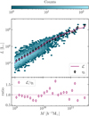 |
Fig. 5. Hexbin scatter plot of (total) [C II] luminosity and halo mass for the emitters in the high-resolution MARIGOLD simulation at z = 5. Solid black symbols show the mean total luminosity computed in narrow mass bins (which coincides with the η1 function also shown in Fig. 4 as a dotted gold line). The solid dark pink line shows the function ℒ(M) obtained applying abundance matching to the simulation output following the steps and assumptions described in Section 3.3. Finally, the ratio of the latter two is shown in the bottom panel. |
Fig. 6 repeats the same analysis but after replacing the total [C II] luminosity with the sum of the squares of the luminosities of the individual emitters. The black symbols here give an estimate of η2(M, z = 5) and the dark pink line is [ℒ(M)]2 (with ℒ taken from Fig. 5). The bottom panel shows that these two functions agree very well at large masses, while ℒ2 underestimates the second moment of the CLF by a factor of ∼2 for M < 1010 h−1 M⊙. This result suggests that our approach might slightly underpredict the amplitude of the shot-noise term in the power spectrum when all halo masses are considered.
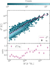 |
Fig. 6. As in Fig. 5, but for the second moment of the CLF. In this case, the black diamonds and the dark pink line show the functions η2 and ℒ2, respectively. |
In summary, we find that the functions ℒ and ℒ2 obtained with abundance matching provide a sound approximation to η1 and η2. The main reasons for this success are: (i) the total [C II] luminosity is dominated by the central galaxy at all halo masses, and (ii) the scatter in luminosity at fixed halo mass remains moderate, although it increases toward lower halo masses, where the effects of bursty star formation may become more pronounced (see also Liu et al. 2024).
4. LIM power spectrum
4.1. EoR-Spec on FYST
As an example of current technology for LIM experiments, we use the specifications of the Epoch of Reionization Spectrometer (EoR-Spec, Nikola et al. 2023; Freundt et al. 2024) that will be deployed on FYST. Prime-Cam–one of the two first-generation instruments that will be installed on FYST by the CCAT-prime collaboration–will have an unprecedented mapping speed at the target wavelengths (CCAT-Prime Collaboration 2023). In its cryostat, it will hold up to seven instrument modules (five cameras working at different frequencies and two EoR-spec modules), each with a field of view of 1.3 square degrees.
EoR-Spec consists of an optical system made of four silicon lenses and several filters, a scanning Fabry-Perot interferometer (FPI), and three hexagonal arrays of Microwave Kinetic Inductance Detectors (MKIDs) sensitive to both polarisations. Over 5 years, this imaging spectrometer will perform the DSS, namely a LIM survey of [C II] over two patches4 of the sky (4 square degrees each) covering the Extended-COSMOS (Aihara et al. 2018) and the Extended Chandra Deep Field South fields (Lehmer et al. 2005), whose first light is expected in 2026. Observations will be conducted in two frequency bands, 210−315 GHz (5.033 < z < 8.050 for [C II]) and 315−420 GHz (3.525 < z < 5.033), with a resolving power of R ∼ 100 over the whole spectral range. The two frequency intervals are observed simultaneously by picking the second- and third-order fringes of the FPI for the low- and high-frequency bands, respectively. Two of the MKID arrays will cover the low-frequency band and the third one will cover the high-frequency band. At any given time, the observed frequency will change as a function of the distance from the centre of the array due to the light incidence angle. Basically, there will be rings of detectors that see the same frequency across the arrays, with increasing frequency outwards (see Fig. 12 in Nikola et al. 2022). The sequence of telescope sky scans and the FPI frequency scans will be optimised to obtain uniform coverage of the survey volume with a total observing time of tsurv ≃ 4000 hours (Cothard et al. 2020; CCAT-Prime Collaboration 2023). Around 15 FPI steps are needed to fill in all frequencies.
4.2. Survey characteristics
4.2.1. Survey volume
Since a statistically significant detection of the PS with EoR-Spec with modest contamination from interlopers is expected only at the highest frequencies (e.g. Karoumpis et al. 2022; Clarke et al. 2024), we follow previous studies and consider a 40 GHz interval centred around 410 GHz (corresponding to z ≃ 3.6355) and thus covering the redshift range 3.42 < z < 3.87. In our reference cosmology, this corresponds to a comoving radial distance in redshift space of Δr∥ ≃ 240 h−1 Mpc.
Setting competitive constraints on the LF of the [C II] emitters requires sampling large areas at high sensitivity. For this reason, we consider an abstract future survey that covers a larger area than the currently planned DSS and further discuss how results vary as a function of the survey size and sensitivity. The only assumption we make is that progress with manufacturing on-chip spectrometers and developing novel readout technologies will allow us to achieve the same sensitivity of DSS. The smallest survey area we take in consideration is Ωsurv = 16 sq. deg., a configuration which has been already studied in the literature as it was the planned area of an earlier version of the DSS (Karoumpis et al. 2022). In this case, the survey extends for Δr⊥ ≃ 332 h−1 comoving Mpc in the direction perpendicular to the line of sight (assuming a compact geometry on the sky with angular extension  ).
).
4.2.2. Spatial resolution of the intensity maps
The finite resolution of the observational setup smooths the measured intensity field over a characteristic angular and spectral scale. In Fourier space, this corresponds to a damping of the measured power spectrum, which can be written as
 (20)
(20)
where W⊥ and W∥ are window functions that account for resolution effects transverse and parallel to the line of sight, respectively, and Wvox accounts for the fact that observations taken at different times are averaged into a single value within each individual spatial and spectral pixels during the map-makingprocess.
The instrument beam, which we assume to be Gaussian, has a full width at half maximum (FWHM) of ΔθFWHM = 33 arcsec. At the redshift of interest, this angular resolution corresponds to a transverse comoving size of Δ⊥FWHM = dA(z) ΔθFWHM ≃ 0.76 h−1 Mpc, where dA(z) is the comoving angular diameter distance (equal to the comoving radial distance in a flat universe). For a Gaussian beam, the smoothing effect on the power spectrum is described by the transverse window function
 (21)
(21)
where  . In our setup, this yields σ⊥ ≃ 0.32 h−1 Mpc at the central frequency, implying that attenuation becomes significant for transverse wavenumbers k⊥ ≳ σ⊥−1 ≃ 3.1 h Mpc−1. For instance, at k⊥ = π/Δ⊥FWHM ≃ 4.13 h Mpc−1, the window function evaluates to W⊥ ≃ 0.17.
To produce a well-sampled map that faithfully captures all relevant spatial features, individual measurements–each covering overlapping regions of the sky–are combined and interpolated onto a regular grid with pixel size δ⊥ that is at most half the angular resolution, that is, δ⊥ ≤ Δ⊥FWHM/2, in accordance with the Nyquist-Shannon sampling criterion5. The angular sampling factor η⊥ = Δ⊥FWHM/δ⊥ quantifies how finely the sky is sampled and corresponds to the number of pixels per resolution element. Nyquist sampling corresponds to η⊥ = 2, while values greater than two indicate oversampling, which enhances the fidelity of the reconstructed map without improving its intrinsic resolution. A common choice is η⊥ ≃ 3 (e.g. Sullivan et al. 2025). As a result, for each angular dimension on the sky, the accessible wavenumbers in Fourier space are integer multiples of the fundamental mode kf⊥ = 2π/Δr⊥ ≃ 0.019 h Mpc−1 and information on the intensity field is available up to the Nyquist wavenumber, kN⊥ = π/δ⊥ = η⊥ π/Δ⊥FWHM = 4.13 η⊥ h Mpc−1. Beyond this limit, the discrete sampling introduces aliasing, rendering signal reconstruction unreliable.
Similar considerations apply to the sampling of fluctuations along the line of sight. A FPI transmits radiation with a frequency-dependent response that is well approximated by a Lorentzian profile6 which is characterised by the central frequency νo and a FWHM of Δνo = νo/R. This frequency width corresponds to a comoving radial resolution of
 (22)
(22)
which evaluates to Δ∥FWHM ≃ 24.54 (100/R) h−1 Mpc at the central frequency of the survey. The frequency response of the spectrometer suppresses the PS along the line of sight by the factor
 (23)
(23)
which reduces to W∥ ≃ 1 − |k∥| Δ∥FWHM + k∥2 (Δ∥FWHM)2/2 when k∥ → 0. In the LIM literature, following the approach of Li et al. (2016), several authors approximate the line-of-sight window function W∥ with a Gaussian damping factor of the form WG = e−μ2k2σ∥2, where σ∥ ≃ Δ∥FWHM/2.355. While this expression provides a convenient analytical form, it does not accurately capture the behaviour of the true window function for FPI spectrometers. In particular, since WG ≃ 1 − k∥2σ∥2 in the limit k∥ → 0, it underestimates the damping of the signal on large scales for surveys with moderate spectral resolution, such as those carried out with EoR-Spec. For instance, at k∥ = 1/Δ∥FWHM, the exponential function in Eq. (23) yields a value of 0.37, while the Gaussian approximation gives 0.65, substantially overestimating the transmitted power.
To ensure a well-sampled map in the spectral dimension, the frequency channel spacing δν should be at most half of the spectral FWHM, i.e. δν < Δνo/2 (corresponding to the comoving radial length δ∥). The spectral sampling factor is defined as η∥ = Δ∥FWHM/δ∥. With this setup, the fundamental wavenumber along the line of sight is kf∥ = 2π/Δr∥ ≃ 0.026 h Mpc−1 while the Nyquist wavenumber is kN∥ = π/δ∥ > η∥ π/Δ∥FWHM ≃ 0.13 (R/100) η∥ h Mpc−1.
Finally, we briefly discuss the voxel window function, which introduces an additional damping factor to the power spectrum. In general, this function can be complex, as it depends on various factors such as the telescope’s scanning strategy, pixel geometry, beam shape, and the spectral response of the instrument (see Appendix A for a detailed discussion). As a first approximation, and assuming the flat-sky limit with regularly spaced voxels, we model the voxel window function as a product of squared sinc functions along each Cartesian direction:
![Mathematical equation: $$ \begin{aligned} W_{\rm vox}(\mathbf k ) = \prod _{i=1}^2 \left[\frac{\sin (k_{\perp ,i}\,\delta _\perp /2)}{k_{\perp ,i}\,\delta _\perp /2}\right]^2\, \left[\frac{\sin (k_\parallel \,\delta _\parallel /2)}{k_\parallel \,\delta _\parallel /2}\right]^2, \end{aligned} $$](/articles/aa/full_html/2025/08/aa54970-25/aa54970-25-eq47.gif) (24)
(24)
where k⊥, i are the Cartesian components of the transverse wavevector. This function remains close to unity for all wavenumbers significantly below the corresponding Nyquist limits. By choosing a typical sampling factor of η⊥ = η∥ ≃ 3, the first zero of the sinc function is pushed well beyond the relevant Fourier modes. We therefore safely neglected this effect and set Wvox = 1.
4.2.3. Direction-averaged power spectrum
In studies of the large-scale structure of the Universe, the anisotropic power spectrum in redshift space Pobs(k, μ) is often expanded in multipole moments with respect to the angle between the wavevector and the line of sight
 (25)
(25)
 (26)
(26)
where ℒℓ denotes the Legendre polynomials. In this study, we focus on the monopole moment of the intensity PS,
 (27)
(27)
which is obtained by averaging Pobs(k, μ, z) over all possible values of μ and, for this reason, is also known as the spherically-averaged power spectrum. Obviously, this quantity can be measured with a higher signal-to-noise ratio (S/N) than Pobs itself.
For surveys that cover a small solid angle on the sky, the line of sight can be considered to be fixed and P(k, μ) = P(k, −μ) so that the integrations in Eq. (27) can be performed between 0 and 1. Modifications are needed when the instrumental setup or selection effects only allow measurements of Pobs for a limited range of μ, however. This applies to the surveys planned with EoR-Spec, where a strong asymmetry between the accessible Fourier modes along and across the line of sight restricts the range over which meaningful averaging can be performed (this is illustrated in Fig. 7 for R = 100 and sub-Nyquist sampling, i.e. η⊥ = η∥ = 1). High values of μ are only possible for k ≲ kN∥, while at much higher wavenumbers all modes have μ ≃ 0 (i.e. k ≃ k⊥ ≫ k∥). We therefore adapted the definition of the monopole moment by introducing the direction-averaged power spectrum,
 (28)
(28)
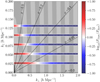 |
Fig. 7. Location in the (k⊥, k∥) plane of the Fourier modes that are available in a 16 sq. deg. survey conducted with EoR-Spec (R = 100) at z ≃ 3.6 and with η⊥ = η∥ = 1 (partially overlapping circles). The colour indicates the ratio of the corresponding clustering and shot-noise contributions to the PS (for our pessimistic LF with α = −1.1). The light and dark grey bands highlight the bins adopted in our analysis (Δk = 5 kf∥ ≃ 0.13 h Mpc−1). These are annuli but appear as vertical bands due to the strong asymmetry in the scales along the axes. The dotted lines denote fixed values of μ = k∥/k. |
where the integrals should be replaced by discrete sums when too few modes are available at fixed k. To implement Eq. (28) for EoR-Spec and prospective future instruments, we set μmin = kf∥/k to approximately account for foreground contamination (see Sect. 4.4), and μmax = min(1, kmax∥/k) with kmax∥ = π/Δ∥FWHM to capture the effects of finite spectral resolution. We adopted this refined treatment in our forecasts, whereas earlier studies (Karoumpis et al. 2022; Clarke et al. 2024) relied on a simplified formulation (cf. Equation 40 in Karoumpis et al. 2022).
4.3. Binning and error budget
In practice, P0 is estimated within finite bins of size Δk. In what follows, we present results obtained using Δk = 5 kf∥ but we have tested that our conclusions do not depend on this choice. The number of independent Fourier modes contributing to each bin can be approximately computed by taking the ratio of the k-space volume of a bin and the volume of a fundamental cell, kf∥ (kf⊥)2, which gives (see Appendix B)
 (29)
(29)
where Vsurv denotes the comoving volume covered by the survey (assumed to be a rectangular cuboid). Only the region with k∥ > 0 is considered as the line intensity is a real-valued quantity and its Fourier modes at k and −k are complex conjugates and thus not independent.
Assuming that both the LIM fluctuations and the detector noise can be approximated as Gaussian random fields, the statistical uncertainty associated with the direction-averaged PS is
 (30)
(30)
where PWN denotes the white-noise power spectrum set by the sensitivity of the instrument. To evaluate PWN for EoR-Spec, we adopted the sensitivity estimate reported in Table 1 of CCAT-Prime Collaboration (2023), expressed as a noise-equivalent intensity7 (NEI) of 98 000 Jy sr for a resolving power R = 100. This value represents a weighted average across the top three weather quartiles, assuming two EoR-Spec modules observe concurrently and that, on average, 80% of the detectors are operational.
For simplicity, we first computed PWN assuming sub-Nyquist sampling with η⊥ = η∥ = 1 (i.e., one voxel per resolution element). If the survey volume is observed uniformly, the white-noise power spectrum is given by
 (31)
(31)
where σvox is the rms noise in a resolution element of comoving volume Vvox, and tvox is the average observing time per voxel per detector.
Assuming a scan strategy that uniformly covers the survey area and allocates equal integration time to each spectral-resolution channel, the average integration time per voxel is
 (32)
(32)
where Nvox = Npix Nν is the total number of voxels with
 (33)
(33)
the number of pixels on the sky and the number of frequency channels, respectively. For our 16 sq. deg. survey with R = 100, we obtain Vvox ≃ 14.3 h−3 Mpc3, Npix ≃ 4102, and Nν ≃ 30 (in the high-frequency band), leading to:
 (34)
(34)
Adopting a finer sampling scheme with η⊥ > 1 and η∥ > 1, the total observing time is divided among more (smaller) voxels, which increases the rms noise per voxel by a factor of η⊥2η∥. The voxel volume decreases by the same factor, however, and leaves PWN unchanged. It is important to note, though, that this finer sampling introduces correlations in the noise between neighbouring voxels, as multiple measurements contribute to each resolution element.
In the following sections, we extend our analysis to include futuristic instruments characterised by a resolving power of R = 500. It is therefore essential to assess how instrumental noise scales with R. According to the radiometer equation, the NEI scales as NEI ∝ Δν−1/2 ∝ R1/2, while the voxel volume behaves as Vvox ∝ Δν ∝ R−1, and the number of frequency channels grows as Nν ∝ R. Consequently, for a fixed total survey duration tsurv, the noise power spectrum scales as PWN ∝ R. It is possible to maintain a constant PWN by increasing tsurv proportionally to R, however.
4.4. Map making, foregrounds, and interlopers
Foreground contamination constitutes a major challenge for LIM studies as it superimposes prominent fluctuations to the target signal. For each experimental setup, the contamination needs be characterised and, if possible, isolated within the data analysis pipeline.
For [C II] experiments, the strongest contaminants are atmospheric noise, the cosmic infrared background (CIB, i.e. the integrated continuum emission from cosmic dust in galaxies), and redshifted CO rotational lines emitted by foreground galaxies. Removing or mitigating the impact of these contaminants possibly introduces systematic effects in the measured summary statistics. For instance, filtering out atmospheric noise during the map-making process can lead to the suppression of the final PS on the largest scales (e.g. Lunde et al. 2024). Although this systematic effect can be corrected by estimating the pipeline transfer function, the suppression becomes rather extreme at low k∥. Additional systematic effects on large scales might be introduced by the corrections for continuum emission. The CIB is highly dominant in terms of intensity but has a smooth dependence on frequency which makes its separation from the highly fluctuating [C II] signal doable using methods that have been originally developed for the 21 cm line. In general, continuum foregrounds mostly affect a few Fourier modes perpendicular to the line of sight with the lowest wavenumbers, i.e. with k∥ ≃ 0 (e.g Switzer et al. 2019; Zhou et al. 2023). This source of contamination can therefore simply be removed by discarding these modes. All these considerations suggest that an approximate method to account for foreground contamination in our forecasts is to only consider Fourier modes above a minimum k∥. In what follows, we only use modes with k∥ ≥ kf∥ (i.e. we discard those with k∥ = 0) which is equivalent to setting k ≥ kf∥ independently of the angular size of the survey (i.e. increasing Ωsurv will reduce σP0 because Vsurv and Nm(k) will grow but will not extend the power-spectrum analysis to smaller values of k corresponding to larger transverse length scales).
Finally, we briefly discuss line interlopers which can also significantly alter the [C II] PS. Many different approaches have been proposed to correct for this contaminant. For instance, acting at the map level, one could mask the voxels that should contain CO emission from galaxies that have been detected in external surveys (Yue et al. 2015; Sun et al. 2018; Béthermin et al. 2022; Karoumpis et al. 2024). While targeted masking has been proven to be successful in mitigating the contamination at the highest frequencies, it also reduces Vsurv (thus increasing the statistical errors on the PS) and convolves the expected signal with a complicated window function which induces correlations between the measurements in different k-bins. Alternatively, working at the PS level, the contamination from interlopers could be characterised by cross-correlating the LIM data with galaxy catalogues or with intensity maps at different frequencies (Wolz et al. 2016; Schaan & White 2021; Keenan et al. 2022; Roy & Battaglia 2024; Bernal & Baleato Lizancos 2025). Lastly, without requiring any external input, one could use the technique of ‘spectral line de-confusion’ which is based on the fact that sources at different redshifts than the target lines will be mapped to the wrong comoving coordinates so that their PS will be highly anisotropic along the k∥ and k⊥ directions (Visbal & Loeb 2010; Lidz & Taylor 2016; Cheng et al. 2016).
Current estimates on the level of contamination depend on assumptions about the CO spectral line energy distribution (SLED; i.e. the relative intensities of the different rotational transitions) in the interloper galaxies. Roy et al. (2023) found that CO interlopers generate a strong bias in the PS at 410 GHz, while several other authors concluded that contamination is severe only below 350 GHz and that fewer than 10% of the voxels need to be masked at 410 GHz (Yue et al. 2015; Béthermin et al. 2022; Karoumpis et al. 2024). Based on this second set of results, we did not modify our forecasts to account for interloper contamination.
4.5. Clustering and shot-noise amplitudes
Our initial goal is to make predictions about the LIM PS that will be detected with EoR-Spec at z ≃ 3.6 based on the halo model presented in Sect. 2 and the abundance-matching technique described in Sect. 3.3. In order to achieve this, however, we have to face the fact that the ALPINE estimates for the LF are only available in the redshift interval 4 < z < 6, meaning that the abundance matching can only be performed at z ≃ 5. Since both observations and simulations suggest that the [C II] LF evolves rather rapidly with time (e.g. Yan et al. 2020; Khatri et al. 2025), assuming that it remains unchanged within the ∼550 Myr intervening between z = 5 and 3.6 seems implausible. The MARIGOLD simulations offer a way out of this dilemma. Fig. 2 in Khatri et al. (2025) shows that the CLF of the simulated [C II] emitters does not change much between redshift 5 and 3. This is also evident in our Fig. 4, where we compare the relation ℒ(M) extracted from the simulations at z = 5 and 4. We thus proceed by assuming that the function ℒ(M) determined from the ALPINE data (see Fig. 4) can be reliably used to compute the LIM PS at z ≃ 3.6 when combined with the evolved halo mass function and halo bias.
In Table 3, we report the mean [C II] intensity, linear bias and effective volume per emitter obtained at z ≃ 3.6 for different models of the [C II] LF (at z = 5). In our pessimistic case, due to the opposite trends of  and b, the clustering signal (
 ), does not vary much with α. It is the highest for α = −1.9 and the lowest for α = −0.5, but it only changes by a factor of 3 overall. The shot-noise term (
 ) also decreases with α and varies even less, with an overall change by a factor of 1.5 when α spans from −1.9 to −0.5. Obviously, our optimistic and pessimistic predictions differ much more and their ratio at fixed α is driven by
  . For α = −1.1, both the clustering and shot-noise amplitudes deviate approximately by a factor of 25.
Parameters derived from the halo model for the LIM PS at z ≃ 3.6 for different input [C II] LF.
It is interesting to note that the effective number of galaxies per voxel  (sometimes called sparsity, Schaan & White 2021) is always well below unity for both R = 100 and 500. This means that only a small fraction of voxels contain a bright galaxy at the redshift of interest. In particular, voxels with more than one such galaxy are extremely rare. This opens interesting perspectives for mitigating the interloper contamination (e.g. Cheng et al. 2020).
4.6. Results
Our results for the PS are presented in the left panels of Fig. 8 for R = 100, and Fig. C.1 for R = 500. Shown is the contribution to the variance of the specific intensity per unit log interval in k
 (35)
(35)
(solid curves) together with its statistical error derived from Eq. (30) assuming Δk = 5kf∥ (shaded areas). Red and blue colours correspond to our optimistic and pessimistic LFs, respectively, both with α = −1.1. While the solid curves trace the theoretical predictions continuously in k, the overlaid symbols show the results obtained with our actual binning scheme.
In all cases, we adopted a fiducial value of σ = 3 h−1 Mpc. This should be regarded as a rough estimate, given the absence of clustering measurements at these redshifts. It is motivated by the following considerations: (i) the line-of-sight pairwise velocity dispersion measured by the 2dF Galaxy Redshift Survey (2dF GRS) for star-forming galaxies in the local Universe is σ12 ∼ 420 km s−1 (Madgwick et al. 2003), which corresponds to a damping parameter  km s−1, or equivalently σ ∼ 3 h−1 Mpc; (ii) the velocity dispersion of DM haloes is expected to scale with mass and redshift as M1/3 H(z)1/3; (iii) our LIM signal at z = 3.6 is dominated by haloes of mass M = a few × 1011 h−1 M⊙, corresponding to a one-dimensional velocity dispersion of ∼160 km s−1 which is slightly higher than that of the haloes hosting the 2dF GRS star-forming galaxies at z = 0 (1012 h−1 M⊙ and ∼130 km s−1); (iv) at high redshift, the large-scale structure of the Universe is less evolved resulting in smaller relative velocities between distinct haloes; and (v) the intrinsic velocity dispersion of the [C II] emitting gas–driven by both ordered rotation and turbulent motions within galaxies (see e.g. Kohandel et al. 2020)–must also be taken into account. Taken together, these considerations suggest that σ should lie within the range 1 − 3 h−1 Mpc, and we adopted the upper end of this interval for our analysis.
The optimistic and pessimistic LFs generate power spectra with similar shapes that, however, differ in amplitude by a factor of ∼25. This gap approximately encompasses the range spanned by the different predictions that have appeared in the literature (Silva et al. 2015; Serra et al. 2016; Dumitru et al. 2019; Chung et al. 2020; Padmanabhan et al. 2022; Kannan et al. 2022; Karoumpis et al. 2022; Sun et al. 2023; Clarke et al. 2024). The individual contributions from the clustering and shot-noise components are indicated with dashed and dot-dashed lines, respectively. In a concrete experimental setting, the white-noise spectrum PWN must be subtracted from the measured signal–or incorporated into the model used to fit the data–in order to isolate P0. For this reason, we also include the white noise PS in the figure (indicated by a dotted line). It is worth noting that Δ2 exceeds the white-noise level at only one data point (two in Fig. C.1), even in the optimistic scenario. This underscores the critical importance of accurately characterising the white noise associated with the instrument in order to reliably isolate the LIM signal.
The right panel of Fig. 8 displays the cumulative S/N for Δ2 as a function of k, based on our binning strategy. In all cases, a detection of the LIM signal should be achievable: the cumulative S/N reaches values of approximately 3.4 in the pessimistic case and up to 54 in the optimistic scenario. These findings are broadly consistent with the recent forecasts for EoR-Spec presented by Karoumpis et al. (2022) and Clarke et al. (2024).
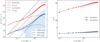 |
Fig. 8. Left: Function Δ2(k, z ≃ 3.6) for our optimistic and pessimistic cases (solid lines) and its statistical uncertainty (shaded regions) estimated for a 16 sq. deg. survey with R = 100. The dotted line shows the white-noise spectrum for EoR-Spec, and the dashed and dot-dashed lines refer to the clustering and shot-noise components, respectively. Right: Cumulative S/N for the spectra shown in the left panel. In both panels, the markers indicate the centre of our k-bins. |
4.6.1. Redshift-space distortions and resolution effects
The power spectra displayed in Fig. 8 present some characteristic features at both small and large scales. In order to explain their origin, we discuss the impact that redshift-space distortions and instrumental effects have on Δ2. By inserting Eqs. (10), (11), (14) and (20) in Eq. (28), we obtain
![Mathematical equation: $$ \begin{aligned} P_0(k,z)=&\bar{I}_\nu ^2(z)\,\left\{ \left[b^2(z)\,\mathcal{F} _0 (k,z)+2\,b(z)f(z)\,\mathcal{F} _2(k,z)\right.\right.\nonumber \\&\left.\left.+f^2(z)\,\mathcal{F} _4(k,z)\right]\,P_{\rm m}(k,z)+\bar{n}^{-1}_{\rm eff}(z)\,\mathcal{G} _0(k,z)\right\} , \end{aligned} $$](/articles/aa/full_html/2025/08/aa54970-25/aa54970-25-eq68.gif) (36)
(36)
with
 (37)
(37)
and
 (38)
(38)
In the absence of instrumental effects (i.e. W⊥ = W∥ = 1), non-linear redshift-space distortions (i.e. σ = 0 or 𝒟 = 1), and when averaging over the full range of μ ∈ [0, 1], the functions ℱ0, ℱ2, ℱ4 and 𝒢0 take on their ‘classical’ values of 1, 1/3, 1/5, and 1, respectively. When μ is restricted to the interval kf∥/k ≤ μ ≤ kmax∥/k, ℱ0 and 𝒢0 remain unchanged; however, ℱ2 and ℱ4 are significantly modified, becoming
 (39)
(39)
 (40)
(40)
and decline rapidly as a function of k. In the low-k regime, this behaviour arises because μmax is fixed to 1, while μmin progressively approaches 0 as k increases. This shift reduces the average values of μ2 and μ4 from unity at k = kf∥ to values approaching the classical ones at k = kmax∥. Conversely, in the high-k regime, where μmax < 1, both the upper and lower bounds of μ decrease with increasing k. As a result, the functions exhibit a more rapid decline in this regime.
Activating non-linear redshift-space distortions further suppresses ℱ2 and ℱ4, while also causing ℱ0 to deviate from unity (see the dotted curves in the left panel of Fig. 9). The suppression of the clustering signal due to the incoherent redshift-space distortions remains mild for the EoR-Spec resolving power of R = 100, with the damping factor 𝒟 confined in the range 0.86 ≤ 𝒟 < 1 (assuming σ = 3 h−1 Mpc) since our setup does not sample Fourier modes with k∥ > kmax∥ ≃ 0.13 h Mpc−1. In contrast, for an hypothetical future spectrograph with R = 500, the damping can be significantly stronger, with 𝒟 reaching values as low as 0.11 when k∥ = kmax∥ ≃ 0.64 h Mpc−1. The function ℱ0 (pink dotted lines) gives the effective damping factor due to the incoherent small-scale motions as a function of k.
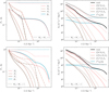 |
Fig. 9. Left: Functions ℱ0, ℱ2, ℱ4, and 𝒢0 defined in Eqs. (37) and (38) for our observational setup, assuming σ = 3 h−1 Mpc and a spectral resolving power of R = 100 (top panel) or R = 500 (bottom panel). The dash-dotted lines represent the analytic approximations given in Eqs. (39) and (40), with colours matching those used for ℱ2 and ℱ4, respectively. Right: Individual components of the LIM power spectrum entering Eq. (36) for our pessimistic luminosity function with α = −1.1 (similar results are found for other LF assumptions). |
Finally, when instrumental effects are taken into account, all the functions are affected in two key ways: (i) they experience significant damping due to the limited spectral resolution, as captured by W∥; and (ii) they are strongly suppressed at k ≳ σ⊥−1 owing to the finite angular resolution of the observations, encoded in W⊥. The resolving power of the spectrograph plays a critical role in modulating these effects. For R = 100, both ℱ0 and 𝒢0 are reduced by a factor of approximately 5 at k ≃ 0.2 h Mpc−1, significantly lowering the amplitude of the observed PS. Moreover, since the FWHM of the Lorentzian line profile exceeds 8σ, the resulting exponential damping becomes so severe that the observed signal carries virtually no sensitivity to σ, making it effectively impossible to place relevant constraints on this parameter at the given spectral resolution. The situation improves substantially for R = 500, where the suppression due to the spectral resolution is less severe and Δ∥FWHM ≃ 1.6σ. In this case, although the damping of the clustering signal due to the incoherent redshift-space distortions remains subdominant, it cannot be neglected entirely, and setting constraints on σ becomes possible.
To mitigate the suppression caused by W∥, we could use a different clustering statistic. One possible approach, involves reducing the value of μmax in Eq. (28) to restrict the analysis to Fourier modes with small |k∥|. For example, one could impose μmax = min(1, kmax∥), where kmax∥ ≪ π/Δ∥FWHM. While this strategy enhances the signal by limiting the contribution from modes strongly affected by spectral resolution, it also leads to increased noise. This is because the averaging would be performed over a smaller subset of Fourier modes, and Nm(k) in Eq. (29) would need to be calculated with kmax∥ replacing π/Δ∥FWHM. In practical terms, this amounts to analysing line-intensity maps with intentionally degraded resolution along the line of sight. The optimal choice of kmax∥ could be determined by maximising the overall S/N of the measurement. However, we find that this strategy yields only modest gains in cumulative S/N (e.g. around 7% for kmax∥ = 0.2 h Mpc−1 and R = 500) and does not lead to tighter constraints on the model parameters. For this reason, we retain the full range range of Fourier modes in the analysis presented throughout the remainder of the paper.
4.6.2. Sensitivity to model parameters
Eq. (36) can be employed to constrain model parameters through template fitting. For a fixed cosmological model, theory of gravity (which determines the growth rate f), and observational setup, the functions ℱ0, ℱ2, ℱ4 and 𝒢0 depend solely on σ. This allows the parameters  and σ to be varied in order to fit the observed data. The dominant clustering contribution to the power spectrum–proportional to ℱ0–is only sensitive to the combination
  and to σ. Additional information on
  and
and  can, in principle, be extracted from the sub-dominant components proportional to ℱ2 and ℱ4, respectively. However, these terms can only be meaningfully constrained if they are sufficiently large compared to the statistical uncertainties of the measurements. Moreover, constraining three parameters in this regime requires multiple well-measured data points. On small scales, where the shot-noise component dominates, the power spectrum is primarily sensitive to the product
  .
.
The solid curves in the right-hand panels of Fig. 9 show the individual contributions to the PS appearing in Eq. (36) for our pessimistic scenario characterised by α = −1.1 and σ = 3 h−1 Mpc. At the centre of our first bin and for R = 100, the components proportional to ℱ0, ℱ2, ℱ4 and 𝒢0 contribute approximately 80.2%, 15.3%, 1.1% and 3.4% of the total signal, respectively. In the second bin, these value change to 81.7%, 3.6%, 0.1%, and 14.6%. As expected, the coherent large-scale flows–encoded in the terms proportional to f and f2–only modestly enhance the clustering signal for highly biased tracers such as [C II] emitters. Nonetheless, the fact that shot noise and multiple clustering terms contribute at comparable levels highlights the necessity of employing statistical inference to disentangle and constrain the individual components of the signal.
5. Bayesian inference
In this section, we assess what information can be extracted about the population of [C II] emitters from the measurements of the LIM PS. The most direct approach is to fit Eq. (36) to the data using  and
and  as tunable parameters while keeping fixed the cosmological parameters (and thus f). This procedure allows us to determine information about the [C II] LF without assuming its functional form and without relying on abundance matching. In fact, Eqs. (5) and (16) show that
  is proportional to the first moment of the LF (
 ) and
) and  gives exactly the second moment. We term this approach minimal modelling and we pursue it in Sects. 5.1 and 5.2.
Alternatively, one could pick a functional form for the LF and set constraints on its free parameters and σ from the LIM PS. In this case, b is a function of the LF parameters which is evaluated via abundance matching and the halo model using Eq. (12). This analysis is presented in Sect. 5.3.
We performed Bayesian inference of the model parameters θ given some mock observations D ≡ {Di} representing the LIM power-spectrum monopole in different k-intervals and/or the LF observed in luminosity bins. We assumed Gaussian independent errors and wrote the likelihood function as
![Mathematical equation: $$ \begin{aligned} \mathcal{L} (\boldsymbol{\theta }|\mathbf D ) \propto \exp \left\{ -\frac{1}{2} \sum _i \frac{\left[D_i-M_i(\boldsymbol{\theta })\right]^2}{\sigma _i^2(\boldsymbol{\theta })}\right\} , \end{aligned} $$](/articles/aa/full_html/2025/08/aa54970-25/aa54970-25-eq83.gif) (41)
(41)
where Mi denotes the model predictions in a given bin and σi is the corresponding statistical errors. We sampled the posterior distribution of θ with the EMCEE code (Foreman-Mackey et al. 2013) which implements the affine-invariant ensemble sampler for Markov chain Monte Carlo (MCMC) by Goodman & Weare (2010). Given the current limited knowledge of the [C II] LF at high redshift (Sect. 3.1), we repeated our analysis several times with different mock data. On the one hand, in our optimistic case, we generated the data based on the Y20 LF. On the other hand, in our pessimistic case, we used our own fit to the LF of the targeted ALPINE detections with α = −1.1. For one particular application, we also considered a steeper faint end, with α = −1.9. In all cases, we assumed that σ = 3 h−1 Mpc.
Table 4 summarises the survey configurations considered in our analysis (labelled A to D). As a baseline (A), we adopted the 16 sq. deg. survey with DSS sensitivity introduced in Sect. 4.2. This reflects the current state of the art, although it already assumes twice the sky area of the planned DSS survey. Building on this, we considered three increasingly ambitious LIM scenarios (B through D), which feature wider sky coverage, enhanced sensitivity, or both, while keeping the spectral resolving power fixed at R = 100. It is important to note that within our modelling framework, variations in Ωsurv or PWN only affect the statistical errors on Δ2 and do not alter the underlying signal or the range of accessible wavenumbers.
Characteristics of the abstract surveys.
Finally, to assess the impact of increased spectral resolution, we also considered variants of each configuration carried out with a futuristic instrument operating at R = 500 (denoted A+ through D+). To ensure a consistent comparison and preserve the white-noise power spectrum level, the total survey duration was scaled up by a factor of five.
5.1. Minimal modelling
Although it would be possible in principle to use  in MCMC sampling, this would lead to a very inefficient exploration of parameter space, because the model parameters are highly correlated. In order to minimise degeneracies and make MCMC sampling much more efficient, were-parametrise the model using
  .
.
We adopted independent uniform priors for all parameters, with the corresponding ranges listed in the upper section of Table 5. For the clustering and shot-noise amplitudes, we selected broad intervals extending from zero to large values. These choices have little impact on our inference, as the mock data tightly constrain both parameters. The situation is different for b and σ, which cannot always be determined precisely and whose posteriors may remain prior-dominated depending on the survey configuration. For these parameters, we imposed theoretically motivated bounds that reflect the expected nature of the LIM signal. We assumed that it is primarily generated by galaxies residing in DM haloes with masses in the range 1010 ≤ M ≤ 1013 h−1 M⊙, ensuring a physically plausible and conservative exploration of parameter space. In particular, we only considered massive, biased haloes, and excluded the possibility of anti-biased tracers by restricting b > 1. The lower limit on σ reflects the velocity dispersion expected for central galaxies in low-mass haloes, while the upper limit accounts not only for satellite galaxies in massive haloes but also includes contributions from internal gas motions and relative velocities between distinct haloes (see also Sect. 4.6).
Uniform prior probabilities.
As an example, in Fig. 10, we present the marginalised one- and two-dimensional posterior distributions of the model parameters obtained for the D and D+ surveys using mock data based on our optimistic LF. The leftmost column of the figure shows that, even in this favourable scenario, it is not possible to place significant constraints on the damping parameter σ when adopting a resolving power of R = 100. At this resolution, the spectral smoothing induced by the instrumental response function W∥ dominates over the physical damping from incoherent redshift-space distortions, rendering variations in σ effectively unobservable. As a result, the posterior distribution for σ remains flat across its prior range, and its degeneracies with other parameters are largely suppressed. In contrast, when the resolving power is increased to R = 500, the damping signature of redshift-space distortions becomes distinguishable from the instrumental effects, which enables us to determine σ. This gain in sensitivity comes with an important caveat, however: The degeneracy between σ and the clustering amplitude parameters, in particular  , becomes significantly more pronounced. This is evident in the shape and orientation of the credible regions in the
  plane. At R = 100, the contours follow the approximate relation
  (in units of 109 h4 Jy2), while for R = 500, the degeneracy tightens along a steeper trajectory,
  . This change reflects the fact that, at high spectral resolution, the observed shape of the power spectrum becomes more sensitive to σ, but in a way that strongly couples to the amplitude of clustering. As a result, uncertainties in σ propagate more directly into
  , elongating the credible regions along a near-linear degeneracy direction. These findings highlight a subtle but important trade-off: While higher spectral resolution enables the measurement of physical parameters like σ, it can also exacerbate parameter degeneracies, particularly when the number of observables remains limited. This suggests that complementary information or additional observables may be required to fully disentangle the contributions of σ, b, and
  to the LIM signal.
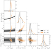 |
Fig. 10. Marginalised posterior distributions of the model parameters we obtained by fitting synthetic data for the LIM PS. The displayed results assume the optimistic [C II] LF and refer to survey D (grey) and D+ (orange). The shaded areas indicate the 68% (dark) and 95% (light) highest posterior density (HPD) regions (hereafter, credible regions). The dotted lines highlight the underlying true values. |
Based on these considerations, we hereafter present results marginalised over σ, unless explicitly stated otherwise. In this section, we focus on the results obtained for R = 100, while the corresponding analysis for surveys with R = 500 is provided in Appendix C.
In Fig. 11, we zoom into the marginalised joint posterior distribution for the clustering and shot-noise amplitudes  and
and  . Here, we overplot the results obtained for the four different surveys described in Table 4. The left and right panels refer to different mock data generated using the optimistic and pessimistic LF, respectively. The axes ranges are different in the two panels. The first thing that one spots is that the peak of the marginalised posterior for
  is shifted from the true value when the optimistic LF is used. This is a projection (or prior-volume) effect which arises because of the degeneracy between
  and σ. The projection of the banana shaped region (see e.g. Fig. 10) generates the shifted peak of the marginalised posterior. The peak of the likelihood lies at the true value, however.
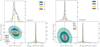 |
Fig. 11. Marginalised posterior distributions of the parameters |


The most important thing we learn from Fig. 11 is how the parameter constraints respond to survey and instrumentation improvements. In order to more easily compare the constraining power of the different surveys, we introduce a figure of merit defined as
![Mathematical equation: $$ \begin{aligned} \mathrm{FoM} =\left[(\det \Sigma _{n})^{-1/2}\,\displaystyle {\prod _{i=1}^n \theta _i^\mathrm{true}}\right]^{1/n}, \end{aligned} $$](/articles/aa/full_html/2025/08/aa54970-25/aa54970-25-eq101.gif) (42)
(42)
with n = 2, in this case, where the symbols θitrue indicate the actual values of the model parameters that have been used to generate the mock data and Σn denotes the corresponding minor of the covariance matrix extracted from the MCMC chains. This dimensionless quantity is a measure of tightness of the posterior probability: the higher is FoM, the stronger are the constraints on the model parameters. For non-correlated variables, it gives the geometric average of their S/N. It turns out that increasing the sensitivity of the survey is more beneficial than increasing its area. With respect to survey A, the FoM increases by a factor of 2.2 (2.6) in the optimistic (pessimistic) case for survey B and of 3.2 (5.6) for survey C. The corresponding figure for survey D is 6.0 (13.3).
Fig. 12 shows the marginalised posterior distribution of the linear bias parameter which provides information about the DM haloes hosting the [C II] emitters. Survey A is incapable of setting any useful constraints on b. In the optimistic case, all the other configurations are sufficient to provide a measurement with a S/N greater than one. In particular, a larger survey area (B) gives tighter constraints than a more sensitive survey (C).Conversely, in the pessimistic case, survey D is needed to measure b.
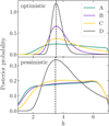 |
Fig. 12. Marginalised posterior distributions for the linear bias parameter of the [C II] emitters. The dotted lines indicate the true values. |
In the left panel of Fig. 13, we present the marginalised posterior distributions for the mean LIM signal,  , which is treated as a derived parameter in our analysis. Since our inference is based on independent uniform priors for the primary model parameters, the resulting effective prior on
  is non-trivial. It features a sharp cutoff at very small intensities, followed by a pronounced peak and a long tail extending toward higher values (see Appendix D). For the optimistic luminosity function, we find that both surveys B and D yield relatively tight posterior distributions for
  , demonstrating the capability of these configurations to constrain the mean LIM intensity. In the more challenging scenario based on the pessimistic luminosity function, however, only survey D shows a marked suppression of the extended high-intensity tail, indicating a genuine gain in constraining power.
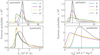 |
Fig. 13. Marginalised posterior distributions for the mean LIM intensity (left) and the effective volume per [C II] emitter (right). The dotted lines indicate the true values. |
Similar conclusions emerge from the analysis of the marginalised posterior distribution of the derived parameter  , shown in the right panel of Fig. 13. While the shot-noise amplitude,
  , is relatively well constrained across all test surveys–with the exception of Survey A under the pessimistic scenario (see Fig. 11)–disentangling and independently constraining the amplitude
  and the effective volume
  of the emitters remains significantly more challenging.
In Sect. 4.6.2, we have demonstrated that redshift-space distortions introduce only per-cent level correction to the PS and that their impact rapidly diminishes with increasing wavenumber. Armed with this knowledge, one might be tempted tosimplify the model for the LIM PS by neglecting the terms proportional to f in Eq. (36) and by setting 𝒟 = 1. The consequences of such a simplification are illustrated in Fig. 14 for the D and D+ surveys using the optimistic LF. We compare the marginalised posterior distributions in the  plane obtained by (i) using the full model, which includes RSDs and marginalises over both b and σ (shaded areas) and (ii) adopting a simplified model that neglects RSDs entirely (solid lines). It is evident that excluding RSDs from the analysis introduces significant biases in parameter estimation, particularly for high-resolution observations with R = 500. Furthermore, the simplified model underestimates the uncertainty on
  , highlighting that accurate modelling of RSDs remains essential, even when their apparent impact on the PS amplitude is modest.
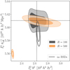 |
Fig. 14. Joint posterior distributions of the clustering and shot-noise amplitudes for the D (grey) and D+ (orange) survey configurations. Shaded regions denote the 68% and 95% credible regions obtained using the full four-parameter model in Eq. (36), which includes redshift-space distortions (RSDs), after marginalising over the parameters b and σ. Unfilled contours show the corresponding credible regions derived from a simplified two-parameter model that neglects RSDs. |
5.2. Moments of the luminosity function
The LIM PS is sensitive to the first two moments of the LF,  and
and  . It is thus interesting to investigate what constraints can be set on these quantities. Eq. (5) shows that
  can be obtained rescaling
  by a (cosmology dependent) constant factor. In Fig. 15, we plot the joint marginalised posterior distribution of
  and
and  by treating them as derived variables in our MCMC chains. The two parameters turn out to be nearlyuncorrelated.
For the optimistic case (left panel), the second moment of the luminosity function is very precisely and accurately measured, while the first moment,  , is also well constrained, particularly in surveys B and D. These two surveys yield nearly unbiased estimates, with survey D achieving a high S/N of 11.7 and a posterior distribution that peaks close to the true value. In the pessimistic case (right panel), the second moment remains tightly constrained (except for survey A), but the posterior for
  becomes broader and moderately biased, reflecting the degeneracies with b and σ, which are poorly constrained (not shown in the figure). Nonetheless, survey D still achieves a detection with S/N ≃ 4.3, and the peak of the posterior is shifted by only 0.84 standard deviations from the true value. We conclude that, while the LIM PS can robustly constrain the second moment of the LF across a wide range of scenarios, the first moment can also be reliably inferred even though mild biases may arise under pessimistic conditions due to parameter degeneracies.
If one is ready to assume that the LF has a particular functional form, then the constraints on the moments can be turned into constraints on the parameters. These will be degenerate if the model for the LF contains more than two parameters. For instance, assuming a Schechter function gives
 (43)
(43)
 (44)
(44)
or, equivalently,
 (45)
(45)
 (46)
(46)
where we have used the relation Γ(1 + x) = x Γ(x). Fig. 16 shows different projections of the degeneracy locus of the LF parameters corresponding to the actual first two momenta of our pessimistic case with α = −1.1 at z = 5 (solid) and 3.6 (dashed). Uncertain constraints on the moments will thus be remapped to posterior distributions with support that elongates along these complex curves.
5.3. Parameters of the luminosity function
A complementary approach, which we adopt in this section, is to constrain a parametric representation of the LF directly from the LIM PS. Specifically, we assume that the LF can be accurately described by a Schechter function and derive the joint posterior distribution of its three parameters, starting from the independent uniform prior distributions listed in the bottom part of Table 5.
By construction, our implementation of this approach is not equivalent to the concept discussed at the end of Sect. 5.2. Indeed, there, we showed that the LIM PS can be used to set constraints of the parameters of the LF at z = 3.6. Conversely, here, to be consistent with the generation of our mock data presented in Sect. 4.5, we perform the abundance matching at z = 5 and we model the power spectra at z ≃ 3.6 by assuming that the function ℒ(M) does not evolve in between. We therefore effectively set constraints on the LF at z = 5, while in this model, the LF at z = 3.6 is not even necessarily well described by a Schechter function8.
An advantage of this framework is that it enables a joint analysis of the LIM PS at z = 3.6 and the ALPINE LF data at z = 5. Because the mock data were generated assuming the pessimistic LF scenario and no redshift evolution in ℒ(M), however, the resulting constraints are intrinsically conservative. They should be interpreted as lower bounds on the performance of this method, with real data expected to yield tighter constraints as measurements improve.
The marginalised posterior distribution of the model parameters given the LIM PS for survey A is represented in the left panel of Fig. 17 using green tones. It is evident that Δ2(k) does not constrain α and that all the LF parameters are strongly correlated. The contours of the posterior probability elongate along the solid degeneracy lines presented in Fig. 16 but are, of course, broader as the moments of the LF are measured with an uncertainty. A careful inspection reveals another small difference: the contours in the {Φ*, L*} plane close at low Φ* (corresponding to α approaching −2) while the corresponding lines in Fig. 16 are unlimited. This happens because, in this region of parameter space, the contribution to  from emitters with L ≪ L* is non-negligible but our halo model only considers haloes with M > 106 h−1 M⊙ and thus truncates the LF at the extreme faint-end (L ≲ 10 L⊙) underestimating
  with respect to the idealised Schechter function.
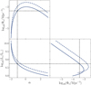 |
Fig. 16. Triplets of the Schechter function parameters (Φ*, L*, and α) that give exactly the same values of the first two moments as our pessimistic LF at z = 5 (solid) and 3.6 (dashed). |
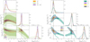 |
Fig. 17. Left: Marginalised posterior distributions of the LF parameters obtained by fitting the LIM PS (green), the number counts of the targeted ALPINE survey (orange), and the combination of the two datasets (violet). The shaded areas indicate the 68% and 95% credible regions. Right: As in the left panel, but for the fit of the combined datasets and for different LIM surveys. |
For comparison, we fit the LF measurements from the ALPINE targeted detections (see Fig. 1) with the same Schechter function. The corresponding posterior distribution is displayed with orange tones in the left panel of Fig. 17. The LF data better constrain the model parameters than the LIM PS: the orange shaded regions are narrower and the marginalised posterior for α shows a clear peak around the true value.
Eventually, we fit the LIM and LF data simultaneously. The resulting posterior distribution is shown in Fig. 17 with violet tones in the left panel. In order to compare the constraining power of the different data with a single number, we introduce a FoM defined analogously to Sect. 5.1 but for three parameters. The ALPINE LF provides constraints that are substantially tighter than the LIM PS (the FoM is a factor 3.9 smaller). However, the combination of the two datasets increases the FoM by a factor of 1.1 with respect to the fit to the LF alone.
In the right panel of Fig. 17, we show the constraints on the Schechter function parameters to the joint LF+PS data for the different surveys. The contours and lines for survey A (teal) coincide with those presented in the left panel (violet) but the plot area is narrower here. Our results show that increasing the sensitivity (survey C) provides a much bigger improvement in the determination of the Schechter parameters with respect to enlarging the survey area (survey B). The marginalised one-dimensional posterior distributions appear all very similar, however. The improvements mostly come from reducing theimportance of the tails.
In Fig. 18, we repeated the analysis using different mock data representing the pessimistic case with α = −1.9. As we have discussed in Sect. 4.5, a steeper faint-end slope corresponds to stronger clustering and shot-noise amplitudes (see Table 3) which increase the S/N of the PS measurements and thus the FoM of the corresponding fit. Since the ALPINE measurements of the LF allow α = −1.9 but do not prefer it (see the orange contours in the left panel of Fig. 17), for our analysis we generated mock LF data that sample a Schechter function with α = −1.9 and have the same relative uncertainties as the ALPINE measurements. In this case, the contours of the posterior distributions given the LF data and given the PS measurements are shifted in Φ* and L* whenever α departs significantly from −1.9. Since they overlap only around the true values, the joint fit PS+LF has a much higher FoM than the individual ones. For survey A, the marginalised uncertainties for the individual parameters (i.e., the standard deviations of the one-dimensional posteriors) are 4.9% for log10[Φ*/Mpc−3], 1.2% for log10(L*/L⊙), and 5.2% for α. For comparison, the corresponding figures for the pessimistic case with α = −1.1 displayed in Fig. 17 are 8.6, 2.4 and 100.7%, respectively.
6. Summary
Measurements of the [C II] LF at high redshift (z ≃ 3 − 5) remain highly uncertain because current observational capabilities are limited. We explored the potential of reconstructing the LF from the LIM PS that will be measured with next-generation instruments. The first challenge we faced was to reliably predict the expected PS signal. To achieve this goal, we combined empirical constraints from the ALPINE survey with theoretical insights from the MARIGOLD simulations (Khatri et al. 2025), which include a detailed model of [C II] emission from early galaxies. By analysing the simulations, we drew the following conclusions.
-
(i)
Although individual DM haloes typically host multiple [C II] emitters, the total [C II] luminosity is dominated by the central galaxy (Fig. 3 and Table 2).
-
(ii)
The abundance-matching technique can be used to statistically connect [C II] emitters to haloes. This yields an excellent approximation for the first two moments of the CLF Figs. 5 and 6).
-
(iii)
The halo-occupation properties of [C II] emitters evolve very little from z = 5 to 3.6 (see e.g. the dotted lines in Fig. 4).
Building on the insights gained from the simulations, we used an abundance match of the [C II] LF observed by the ALPINE survey in the redshift range 4.4 < z < 5.9 to the halo mass function and thereby derived the mean [C II] luminosity as a function of halo mass ℒ(M) (Fig. 4). We bracketed the uncertainty on the LF by considering two different scenarios: an optimistic high-normalisation case based on the data compilation of Y20, and a pessimistic low-normalisation case informed solely by the targeted ALPINE detections. In the latter, the faint-end slope (which remains poorly constrained) was treated as a free parameter.
We then combined the halo model (reviewed in Sect. 2) with the function ℒ(M) to predict the expected LIM PS, for which we incorporated corrections for instrumental and observational effects. To illustrate the current possibilities, we used the specifications of the EoR-Spec instrument, which is soon to be deployed on FYST, as our reference case. The resulting PS at z ≃ 3.6 is shown in Fig. 8.
In the second part of the paper, we presented forecasts for the FYST DSS at z ≃ 3.6 and extended our predictions to include prospective future surveys featuring a broader sky coverage, an enhanced sensitivity, and/or an increased spectral resolving power. The main conclusions from our Bayesian analysis are summarised below.
-
(iv)
The DSS is expected to constrain both the clustering and shot-noise components of the LIM PS with a S/N of approximately 2 or higher, depending on the true underlying LF (Fig. 11). It does not provide sufficient information to constrain the linear bias parameter of the LIM signal, however (Fig. 12). As a result, the first moment of the LF is noticeably biased (Fig. 15). In contrast, the second moment is accurately recovered.
-
(v)
Even for more sensitive and wider surveys, the damping effect due to the non-linear redshift-space distortions cannot be disentangled from the overall LIM signal (Fig. 10). This is primarily due to the limited spectral resolving power of the instrument (R = 100), which induces a strong suppression of the power spectrum along the line of sight that often dominates over the milder damping caused by peculiar velocities (quantified by the parameter σ). As a result, the imprint of redshift-space distortions is largely erased, which makes it difficult to isolate this effect from the measured signal. This also leads to slightly biased constraints on the clustering amplitude (Fig. 11). The shot-noise level, on the other hand, is determined with both high precision and accuracy (in particular for surveys C and D).
-
(vi)
Increasing the resolution to R = 500 allows the damping from redshift-space distortions to become distinguishable from instrumental effects, enabling a constraint on σ. However, this intensifies degeneracies with the clustering amplitude
 and reduces precision (Fig. 10). Importantly, fitting the data with a model that neglects redshift-space distortions leads to substantial biases in both the clustering and shot-noise amplitudes (Fig. 14).
 -
(vii)
Tight and accurate constraints on the first two moments of the LF translate into strong degeneracies when LF models are fitted with more than two free parameters (e.g. the Schechter function; Fig. 16).
-
(viii)
To address this limitation, we adopted an alternative approach by modelling the LF as a Schechter function and directly constraining its free parameters through a joint fit to the PS (e.g. from the DSS) and the LF measurements (e.g. from ALPINE). We found that the overall normalisation, Φ*, and the characteristic luminosity, L*, are both precisely and accurately determined (Figs. 17 and 18), while the faint-end slope, α, remains largely unconstrained unless its true value is close to −2.
-
(ix)
In all scenarios, a survey sensitivity higher by a factor of
 at the same sky coverage yielded substantially tighter constraints than a surveyed area larger by a factor of 10 at fixed sensitivity (Figs. 11, 15, 17 and 18).
These results underscore important design trade-offs in LIM survey planning. Gains in one area, such as a higher spectral resolution, can improve the sensitivity to specific physical effects, like the damping scale from redshift-space distortions. However, these improvements can also amplify degeneracies between key parameters, especially when the number of independent observables is limited. This emphasises the need to optimise survey configurations in the light of the specific scientific objectives being pursued, whether they involve precise measurements of clustering, bias, or luminosity function moments. We plan to return to this issue in future work by exploring systematic strategies for designing LIM surveys tailored to distinct science goals.
See https://lambda.gsfc.nasa.gov/product/expt/lim_experiments.html and references therein.
It is worth mentioning that, at z = 5 there are only two haloes more massive than this in the whole low-res simulation box.
Further multiwavelength coverage of these fields, including grism spectroscopy from the Euclid mission (Euclid Collaboration: Mellier et al. 2025), is planned with many telescopes (CCAT-Prime Collaboration 2023).
The theorem strictly applies to perfectly band-limited signals. However, the LIM signal convolved with a Gaussian beam retains non-zero power at all spatial frequencies, even if that power decays rapidly.
We thank A. Dev, C. Karoumpis, and D. Riechers for pointing this out.
The NEI is defined as the root-mean-square (rms) intensity noise per unit solid angle accumulated in 1 s of integration time, averaged over the instrument’s field of view.
With our assumptions, due to the evolution of the halo mass function between redshift 5 and 3.6, the first and second moments of the LF increase by a factor of a few, which is in the same ballpark of the variations seen in the MARIGOLD simulations.
The actual finesse ℱ of the interferometer, defined as the ratio between the free spectral range (i.e. the frequency spacing between adjacent transmission peaks) and the full width at half maximum (FWHM) of each peak, is given by  .
.
Acknowledgments
The authors warmly thank Christos Karoumpis, Ankur Dev, Dominik Riechers and Frank Bertoldi for helpful discussions about the DSS survey and the CCAT-prime project. The authors gratefully acknowledge the Collaborative Research Center 1601 (SFB 1601 sub-project C6) funded by the Deutsche Forschungsgemeinschaft (DFG, German Research Foundation) – 500700252. They also acknowledge the International Max Planck Research School for Astronomy and Astrophysics (IMPRS A&A) at the Universities of Bonn and Cologne for supporting EM through a research contract. EM and PK are members of the IMPRS A&A, the Bonn Cologne Graduate School (BCGS), and guest researchers at the Max Planck Institute for Radio Astronomy (MPIfR) in Bonn. CP is grateful to SISSA, the University of Trieste, and IFPU, where part of this work was carried out, for hospitality and support.
References
- Aihara, H., Armstrong, R., Bickerton, S., et al. 2018, PASJ, 70, S8 [NASA ADS] [Google Scholar]
- Alonso, D., Bull, P., Ferreira, P. G., & Santos, M. G. 2015, MNRAS, 447, 400 [NASA ADS] [CrossRef] [Google Scholar]
- Anderson, C. J., Luciw, N. J., Li, Y. C., et al. 2018, MNRAS, 476, 3382 [NASA ADS] [CrossRef] [Google Scholar]
- Bauer, J. B., Marsh, D. J. E., Hložek, R., Padmanabhan, H., & Laguë, A. 2021, MNRAS, 500, 3162 [Google Scholar]
- Bernal, J. L., & Baleato Lizancos, A. 2025, Phys. Rev. D, 111, 043539 [Google Scholar]
- Bernal, J. L., & Kovetz, E. D. 2022, A&ARv, 30, 5 [NASA ADS] [CrossRef] [Google Scholar]
- Bernal, J. L., Breysse, P. C., Gil-Marín, H., & Kovetz, E. D. 2019, Phys. Rev. D, 100, 123522 [Google Scholar]
- Bernal, J. L., Caputo, A., & Kamionkowski, M. 2021, Phys. Rev. D, 103, 063523 [NASA ADS] [CrossRef] [Google Scholar]
- Béthermin, M., Fudamoto, Y., Ginolfi, M., et al. 2020, A&A, 643, A2 [Google Scholar]
- Béthermin, M., Gkogkou, A., Van Cuyck, M., et al. 2022, A&A, 667, A156 [NASA ADS] [CrossRef] [EDP Sciences] [Google Scholar]
- Bohr, S., Zavala, J., Cyr-Racine, F.-Y., & Vogelsberger, M. 2021, MNRAS, 506, 128 [CrossRef] [Google Scholar]
- Breysse, P. C., & Rahman, M. 2017, MNRAS, 468, 741 [Google Scholar]
- Breysse, P. C., Kovetz, E. D., & Kamionkowski, M. 2014, MNRAS, 443, 3506 [NASA ADS] [CrossRef] [Google Scholar]
- Breysse, P. C., Kovetz, E. D., & Kamionkowski, M. 2015, MNRAS, 452, 3408 [CrossRef] [Google Scholar]
- Carilli, C. L. 2011, ApJ, 730, L30 [Google Scholar]
- Carniani, S., Maiolino, R., Smit, R., & Amorín, R. 2018, ApJ, 854, L7 [Google Scholar]
- CCAT-Prime Collaboration (Aravena, M., et al.) 2023, ApJS, 264, 7 [NASA ADS] [CrossRef] [Google Scholar]
- Chang, T.-C., Pen, U.-L., Peterson, J. B., & McDonald, P. 2008, Phys. Rev. Lett., 100, 091303 [NASA ADS] [CrossRef] [Google Scholar]
- Cheng, Y.-T., Chang, T.-C., Bock, J., Bradford, C. M., & Cooray, A. 2016, ApJ, 832, 165 [NASA ADS] [CrossRef] [Google Scholar]
- Cheng, Y.-T., de Putter, R., Chang, T.-C., & Doré, O. 2019, ApJ, 877, 86 [Google Scholar]
- Cheng, Y.-T., Chang, T.-C., & Bock, J. J. 2020, ApJ, 901, 142 [NASA ADS] [CrossRef] [Google Scholar]
- CHIME Collaboration (Amiri, M., et al.) 2022, ApJS, 261, 29 [CrossRef] [Google Scholar]
- Chung, D. T., Viero, M. P., Church, S. E., & Wechsler, R. H. 2020, ApJ, 892, 51 [NASA ADS] [CrossRef] [Google Scholar]
- Clarke, J., Karoumpis, C., Riechers, D., et al. 2024, A&A, 689, A101 [NASA ADS] [CrossRef] [EDP Sciences] [Google Scholar]
- Comaschi, P., & Ferrara, A. 2016, MNRAS, 455, 725 [Google Scholar]
- Cothard, N. F., Choi, S. K., Duell, C. J., et al. 2020, J. Low Temp. Phys., 199, 898 [Google Scholar]
- De Looze, I., Cormier, D., Lebouteiller, V., et al. 2014, A&A, 568, A62 [NASA ADS] [CrossRef] [EDP Sciences] [Google Scholar]
- Decarli, R., Walter, F., Gónzalez-López, J., et al. 2019, ApJ, 882, 138 [Google Scholar]
- Dumitru, S., Kulkarni, G., Lagache, G., & Haehnelt, M. G. 2019, MNRAS, 485, 3486 [NASA ADS] [CrossRef] [Google Scholar]
- Euclid Collaboration (Mellier, Y., et al.) 2025, A&A, 697, A1 [Google Scholar]
- Faisst, A. L., Schaerer, D., Lemaux, B. C., et al. 2020, ApJS, 247, 61 [NASA ADS] [CrossRef] [Google Scholar]
- Foreman-Mackey, D., Hogg, D. W., Lang, D., & Goodman, J. 2013, PASP, 125, 306 [Google Scholar]
- Freundt, R., Li, Y., Henke, D., et al. 2024, SPIE Conf. Ser., 13102, 131020U [Google Scholar]
- Furlanetto, S. R., Oh, S. P., & Briggs, F. H. 2006, Phys. Rep., 433, 181 [Google Scholar]
- Goldsmith, P. F., Langer, W. D., Pineda, J. L., & Velusamy, T. 2012, ApJS, 203, 13 [Google Scholar]
- Gong, Y., Cooray, A., Silva, M., et al. 2012, ApJ, 745, 49 [NASA ADS] [CrossRef] [Google Scholar]
- Goodman, J., & Weare, J. 2010, Commun. Appl. Math. Comput. Sci., 5, 65 [Google Scholar]
- Gruppioni, C., Béthermin, M., Loiacono, F., et al. 2020, A&A, 643, A8 [NASA ADS] [CrossRef] [EDP Sciences] [Google Scholar]
- Gullberg, B., De Breuck, C., Vieira, J. D., et al. 2015, MNRAS, 449, 2883 [Google Scholar]
- Hogan, C. J., & Rees, M. J. 1979, MNRAS, 188, 791 [NASA ADS] [Google Scholar]
- Ihle, H. T., Borowska, J., Cleary, K. A., et al. 2022, ApJ, 933, 185 [NASA ADS] [CrossRef] [Google Scholar]
- Kannan, R., Smith, A., Garaldi, E., et al. 2022, MNRAS, 514, 3857 [CrossRef] [Google Scholar]
- Karkare, K. S., & Bird, S. 2018, Phys. Rev. D, 98, 043529 [Google Scholar]
- Karoumpis, C., Magnelli, B., Romano-Díaz, E., Haslbauer, M., & Bertoldi, F. 2022, A&A, 659, A12 [NASA ADS] [CrossRef] [EDP Sciences] [Google Scholar]
- Karoumpis, C., Magnelli, B., Romano-Díaz, E., et al. 2024, A&A, 691, A262 [NASA ADS] [CrossRef] [EDP Sciences] [Google Scholar]
- Keating, G. K., Marrone, D. P., Bower, G. C., et al. 2016, ApJ, 830, 34 [NASA ADS] [CrossRef] [Google Scholar]
- Keating, G. K., Marrone, D. P., Bower, G. C., & Keenan, R. P. 2020, ApJ, 901, 141 [NASA ADS] [CrossRef] [Google Scholar]
- Keenan, R. P., Keating, G. K., & Marrone, D. P. 2022, ApJ, 927, 161 [Google Scholar]
- Khatri, P., Porciani, C., Romano-Díaz, E., Seifried, D., & Schäbe, A. 2024, A&A, 688, A194 [NASA ADS] [CrossRef] [EDP Sciences] [Google Scholar]
- Khatri, P., Romano-Díaz, E., & Porciani, C. 2025, A&A, 697, A174 [NASA ADS] [CrossRef] [EDP Sciences] [Google Scholar]
- Kohandel, M., Pallottini, A., Ferrara, A., et al. 2020, MNRAS, 499, 1250 [Google Scholar]
- Koprowski, M. P., Dunlop, J. S., Michałowski, M. J., et al. 2017, MNRAS, 471, 4155 [Google Scholar]
- Kovetz, E. D., Viero, M. P., Lidz, A., et al. 2017, ArXiv e-prints [arXiv:1709.09066] [Google Scholar]
- Lagache, G., Cousin, M., & Chatzikos, M. 2018, A&A, 609, A130 [NASA ADS] [CrossRef] [EDP Sciences] [Google Scholar]
- Le Fèvre, O., Béthermin, M., Faisst, A., et al. 2020, A&A, 643, A1 [Google Scholar]
- Lehmer, B. D., Brandt, W. N., Alexander, D. M., et al. 2005, ApJS, 161, 21 [NASA ADS] [CrossRef] [Google Scholar]
- Leo, M., Baugh, C. M., Li, B., & Pascoli, S. 2018, JCAP, 2018, 010 [Google Scholar]
- Leung, T. K. D., Olsen, K. P., Somerville, R. S., et al. 2020, ApJ, 905, 102 [NASA ADS] [CrossRef] [Google Scholar]
- Lewis, A., Challinor, A., & Lasenby, A. 2000, ApJ, 538, 473 [Google Scholar]
- Li, T. Y., Wechsler, R. H., Devaraj, K., & Church, S. E. 2016, ApJ, 817, 169 [NASA ADS] [CrossRef] [Google Scholar]
- Li, W., Xu, H., Ma, Z., et al. 2019, MNRAS, 485, 2628 [Google Scholar]
- Lidz, A., & Taylor, J. 2016, ApJ, 825, 143 [NASA ADS] [CrossRef] [Google Scholar]
- Lidz, A., Zahn, O., Furlanetto, S. R., et al. 2009, ApJ, 690, 252 [NASA ADS] [CrossRef] [Google Scholar]
- Lidz, A., Furlanetto, S. R., Oh, S. P., et al. 2011, ApJ, 741, 70 [NASA ADS] [CrossRef] [Google Scholar]
- Liu, L.-J., Sun, G., Chang, T.-C., Furlanetto, S. R., & Bradford, C. M. 2024, ApJ, 974, 175 [Google Scholar]
- Loiacono, F., Decarli, R., Gruppioni, C., et al. 2021, A&A, 646, A76 [EDP Sciences] [Google Scholar]
- Lunde, J. G. S., Stutzer, N. O., Breysse, P. C., et al. 2024, A&A, 691, A335 [NASA ADS] [CrossRef] [EDP Sciences] [Google Scholar]
- Lupi, A., Bovino, S., Capelo, P. R., Volonteri, M., & Silk, J. 2018, MNRAS, 474, 2884 [NASA ADS] [CrossRef] [Google Scholar]
- Madau, P., Meiksin, A., & Rees, M. J. 1997, ApJ, 475, 429 [NASA ADS] [CrossRef] [Google Scholar]
- Madgwick, D. S., Hawkins, E., Lahav, O., et al. 2003, MNRAS, 344, 847 [Google Scholar]
- Malhotra, S. 2001, ESA Spec. Publ., 460, 155 [Google Scholar]
- Masui, K. W., Switzer, E. R., Banavar, N., et al. 2013, ApJ, 763, L20 [Google Scholar]
- Moradinezhad Dizgah, A., & Keating, G. K. 2019, ApJ, 872, 126 [Google Scholar]
- Moradinezhad Dizgah, A., Nikakhtar, F., Keating, G. K., & Castorina, E. 2022, JCAP, 2022, 026 [Google Scholar]
- Muñoz, J. B., Dvorkin, C., & Cyr-Racine, F.-Y. 2020, Phys. Rev. D, 101, 063526 [CrossRef] [Google Scholar]
- Nikola, T., Choi, S. K., Duell, C. J., et al. 2022, SPIE Conf. Ser., 12190, 121900G [Google Scholar]
- Nikola, T., Stacey, G. J., Freundt, R. G., et al. 2023, in Physics and Chemistry of Star Formation: The Dynamical ISM Across Time and Spatial Scales, eds. V. Ossenkopf-Okada, R. Schaaf, I. Breloy, & J. Stutzki, 352 [Google Scholar]
- Olsen, K., Greve, T. R., Narayanan, D., et al. 2017, ApJ, 846, 105 [Google Scholar]
- Padmanabhan, H. 2018, MNRAS, 475, 1477 [NASA ADS] [CrossRef] [Google Scholar]
- Padmanabhan, H. 2019, MNRAS, 488, 3014 [CrossRef] [Google Scholar]
- Padmanabhan, H. 2023, MNRAS, 523, 3503 [Google Scholar]
- Padmanabhan, H., Breysse, P., Lidz, A., & Switzer, E. R. 2022, MNRAS, 515, 5813 [NASA ADS] [CrossRef] [Google Scholar]
- Parimbelli, G., Scelfo, G., Giri, S. K., et al. 2021, JCAP, 2021, 044 [CrossRef] [Google Scholar]
- Paul, S., Santos, M. G., Chen, Z., & Wolz, L. 2023, ArXiv e-prints [arXiv:2301.11943] [Google Scholar]
- Peacock, J. A., & Dodds, S. J. 1994, MNRAS, 267, 1020 [NASA ADS] [Google Scholar]
- Pineda, J. L., Langer, W. D., & Goldsmith, P. F. 2014, A&A, 570, A121 [NASA ADS] [CrossRef] [EDP Sciences] [Google Scholar]
- Popping, G., van Kampen, E., Decarli, R., et al. 2016, MNRAS, 461, 93 [NASA ADS] [CrossRef] [Google Scholar]
- Pullen, A. R., Chang, T.-C., Doré, O., & Lidz, A. 2013, ApJ, 768, 15 [NASA ADS] [CrossRef] [Google Scholar]
- Pullen, A. R., Doré, O., & Bock, J. 2014, ApJ, 786, 111 [NASA ADS] [CrossRef] [Google Scholar]
- Pullen, A. R., Serra, P., Chang, T.-C., Doré, O., & Ho, S. 2018, MNRAS, 478, 1911 [NASA ADS] [CrossRef] [Google Scholar]
- Riechers, D. A., Pavesi, R., Sharon, C. E., et al. 2019, ApJ, 872, 7 [Google Scholar]
- Righi, M., Hernández-Monteagudo, C., & Sunyaev, R. A. 2008, A&A, 478, 685 [NASA ADS] [CrossRef] [EDP Sciences] [Google Scholar]
- Roy, A., & Battaglia, N. 2024, ApJ, 969, 2 [Google Scholar]
- Roy, A., Valentín-Martínez, D., Wang, K., Battaglia, N., & van Engelen, A. 2023, ApJ, 957, 87 [NASA ADS] [CrossRef] [Google Scholar]
- Sameie, O., Benson, A. J., Sales, L. V., et al. 2019, ApJ, 874, 101 [Google Scholar]
- Schaan, E., & White, M. 2021, JCAP, 2021, 068 [CrossRef] [Google Scholar]
- Schaerer, D., Ginolfi, M., Béthermin, M., et al. 2020, A&A, 643, A3 [NASA ADS] [CrossRef] [EDP Sciences] [Google Scholar]
- Schneider, A., Smith, R. E., & Reed, D. 2013, MNRAS, 433, 1573 [CrossRef] [Google Scholar]
- Scott, D., & Rees, M. J. 1990, MNRAS, 247, 510 [NASA ADS] [Google Scholar]
- Serra, P., Doré, O., & Lagache, G. 2016, ApJ, 833, 153 [NASA ADS] [CrossRef] [Google Scholar]
- Sheth, R. K., Mo, H. J., & Tormen, G. 2001, MNRAS, 323, 1 [NASA ADS] [CrossRef] [Google Scholar]
- Silva, M. B., Santos, M. G., Gong, Y., Cooray, A., & Bock, J. 2013, ApJ, 763, 132 [NASA ADS] [CrossRef] [Google Scholar]
- Silva, M., Santos, M. G., Cooray, A., & Gong, Y. 2015, ApJ, 806, 209 [NASA ADS] [CrossRef] [Google Scholar]
- Stacey, G. J., Hailey-Dunsheath, S., Ferkinhoff, C., et al. 2010, ApJ, 724, 957 [NASA ADS] [CrossRef] [Google Scholar]
- Stutzer, N. O., Lunde, J. G. S., Breysse, P. C., et al. 2024, A&A, 691, A336 [NASA ADS] [CrossRef] [EDP Sciences] [Google Scholar]
- Suginohara, M., Suginohara, T., & Spergel, D. N. 1999, ApJ, 512, 547 [Google Scholar]
- Sullivan, R. M., Hergt, L. T., & Scott, D. 2025, Res. Notes Am. Astron. Soc., 9, 43 [Google Scholar]
- Sun, G., Moncelsi, L., Viero, M. P., et al. 2018, ApJ, 856, 107 [NASA ADS] [CrossRef] [Google Scholar]
- Sun, G., Mas-Ribas, L., Chang, T.-C., et al. 2023, ApJ, 950, 40 [Google Scholar]
- Switzer, E. R., Anderson, C. J., Pullen, A. R., & Yang, S. 2019, ApJ, 872, 82 [NASA ADS] [CrossRef] [Google Scholar]
- Vallini, L., Gallerani, S., Ferrara, A., Pallottini, A., & Yue, B. 2015, ApJ, 813, 36 [NASA ADS] [CrossRef] [Google Scholar]
- Visbal, E., & Loeb, A. 2010, JCAP, 2010, 016 [CrossRef] [Google Scholar]
- Visbal, E., Haiman, Z., & Bryan, G. L. 2015, MNRAS, 450, 2506 [NASA ADS] [CrossRef] [Google Scholar]
- Wolz, L., Tonini, C., Blake, C., & Wyithe, J. S. B. 2016, MNRAS, 458, 3399 [Google Scholar]
- Wolz, L., Pourtsidou, A., Masui, K. W., et al. 2022, MNRAS, 510, 3495 [NASA ADS] [CrossRef] [Google Scholar]
- Wyithe, J. S. B., & Loeb, A. 2007, MNRAS, 375, 1034 [Google Scholar]
- Yan, L., Sajina, A., Loiacono, F., et al. 2020, ApJ, 905, 147 [Google Scholar]
- Yue, B., Ferrara, A., Pallottini, A., Gallerani, S., & Vallini, L. 2015, MNRAS, 450, 3829 [NASA ADS] [CrossRef] [Google Scholar]
- Zhou, X., Gong, Y., Deng, F., et al. 2023, MNRAS, 521, 278 [CrossRef] [Google Scholar]
Appendix A: Line profile from FPI scans
In the lossless approximation, the fraction of incident intensity transmitted by a Fabry-Pérot Interferometer (FPI) at a fixed cavity spacing is described by the Airy function:
 (A.1)
(A.1)
where the coefficient of finesse9 is F = 4ℛ/(1 − ℛ)2 and depends on the mirror reflectivity ℛ. The phase shift between successive internally reflected beams is
 (A.2)
(A.2)
where d is the physical separation of the mirrors, n is the refractive index of the medium between them, ν is the frequency of the incoming light, and θ is the external incidence angle. Resonances occur when δ = 2πm, with m an integer corresponding to the interference order.
Near a resonance at frequency ν0, the transmission function is well approximated by a peak-normalised Lorentzian
 (A.3)
(A.3)
where the FWHM is Γ = ν0/(mℱ), yielding a resolving power R = mℱ. The corresponding area-normalised line profile is
 (A.4)
(A.4)
which, when translated into comoving radial distance r, becomes
 (A.5)
(A.5)
where Δ∥FWHM is the FWHM expressed in comoving distance units. Its Fourier transform is
 (A.6)
(A.6)
which leads to a window function for the power spectrum:
 (A.7)
(A.7)
As discussed in Sect. 4.2.2, this exponential suppression significantly damps the clustering signal on small radial scales, particularly in the presence of low resolving power.
If the FPI is scanned over a sequence of discrete frequency steps, which are subsequently combined to construct an intensity map in voxels, then the effective line profile can be approximated as a sum of Lorentzian functions, each centred at a different frequency step. This results in a multi-peaked or broadened profile, depending on the number of steps and their spacing relative to the FWHM of the individual Lorentzian.
If the system throughput (e.g., atmospheric transmission) or the integration time varies across the scanning process, each Lorentzian should be weighted accordingly. Denoting by νi the centre of the i-th scan step and by wi the corresponding weight, the composite line profile for a voxel centred at ν0 can be written as
 (A.8)
(A.8)
where L(ν; νi) denotes a Lorentzian profile centred at νi. The resulting window function in Fourier space becomes
 (A.9)
(A.9)
where ri is the comoving distance corresponding to νi. This structure can lead to a non-trivial modulation of the damping depending on the scanning scheme.
Further analytic insight can be obtained by assuming uniform weights (wi = 1/N), implying negligible variations in system throughput and equal integration time across all steps. If the scan steps are evenly spaced in frequency by Δνstep, the summation in Eq. (A.9) produces a comb-like interference pattern that modulates the baseline Lorentzian damping. In the limit of large N, the discrete scan approximates a continuous sweep, resulting in a convolution of the Lorentzian with a top-hat function. This leads to the approximate window function:
![Mathematical equation: $$ \begin{aligned} W_\parallel (k_\parallel ) = e^{-|k_\parallel |\,\Delta _\parallel ^\mathrm{FWHM}} \, \left[\frac{\sin (k_\parallel \,\delta _\parallel /2)}{k_\parallel \,\delta _\parallel /2}\right]^2\;, \end{aligned} $$](/articles/aa/full_html/2025/08/aa54970-25/aa54970-25-eq137.gif) (A.10)
(A.10)
where δ∥ is the comoving length corresponding to the total scanned frequency range that is mapped to a frequency channel. For finite N, the sinc modulation becomes more structured, resulting in additional suppression at large |k∥|.
Appendix B: Number of Fourier modes
Let us consider a real-valued field defined within a rectangular cuboid of size (L⊥, L⊥, L∥) and volume V = L⊥2L∥, assuming periodic boundary conditions. The Fourier transform of such a field yields discrete wavevectors of the form k = (i, kf⊥, j, kf⊥, ℓ, kf∥), where (i, j, ℓ)∈ℤ3 and  defines the fundamental mode in each direction. Basically, each discrete mode occupies a cell of volume
  in Fourier space. Due to the Hermitian symmetry of the Fourier transform, only half of the modes carry independent information. The number of independent modes within a thin spherical shell of radius k and thickness Δk ≪ k can be estimated by dividing the volume of the shell Kshell = 2π k2Δk (accounting for the hemisphere) by Kf, yielding the classical result:
 (B.1)
(B.1)
However, if the parallel component of the wavevector is restricted to |k∥|≤k∥max, then the available volume within the shell must be reduced accordingly. Specifically, for k > k∥max, a spherical cap of volume 2π k (k − k∥max) Δk must be subtracted from the hemisphere. As a result, the effective shell volume becomes:
 (B.2)
(B.2)
The number of available modes per bin then reads:
 (B.3)
(B.3)
Appendix C: Results with R = 500
In this appendix, we present a set of figures analogous to those shown in Sect. 5.1 of the main text, but corresponding to a spectral resolving power of R = 500 instead of the baseline value of R = 100. This allows us to assess the impact of increased spectral resolution on the various quantities of interest.
Appendix D: Marginal prior for the mean intensity
Let us consider two model parameters x > 0 and y > 0 with independent uniform priors on x ∈ [xmin, xmax] and y ∈ [ymin, ymax]. The effective prior on the derived parameter
must be computed by marginalising over the joint prior distribution
 (D.1)
(D.1)
where p(x, y) assumes the constant value A = [(xmax − xmin) (ymax − ymin)]−1 within the prior ranges and vanishes otherwise. To compute the marginal prior for z, we must integrate over y, applying the constraint that x = z2y2 remains within the allowed range:

However, y must also satisfy y ∈ [ymin, ymax], so the integration bounds become
![Mathematical equation: $$ \begin{aligned} y \in \left[ \max \left(y_{\rm min}, \sqrt{\frac{x_{\rm min}}{z^2}} \right), \min \left(y_{\rm max}, \sqrt{\frac{x_{\rm max}}{z^2}} \right) \right]. \end{aligned} $$](/articles/aa/full_html/2025/08/aa54970-25/aa54970-25-eq146.gif)
Inserting the appropriate values from the main text for  , y = b, and
  , this yields
 (D.2)
(D.2)
with A = (6 × 10¹⁰ h2 Jy)−1. The effective prior thus peaks at  Jy (which is close to the true value for the optimistic case), grows linearly with
  for smaller values, and drops off approximately as
  for larger values until it vanishes at
  Jy.
Jy.
A similar approach can be used to derive the marginalised prior on  ; however, we omit the detailed calculations here, as the resulting expressions are rather lengthy and cumbersome.
All Tables
Parameters derived from the halo model for the LIM PS at z ≃ 3.6 for different input [C II] LF.
All Figures
|
Fig. 1. [C II] LF estimated from the targeted ALPINE detections by Yan et al. (2020, Y20) (black data points and error bars). We show the average between the estimates at redshift z ∼ 4.5 and 5.5. Our Schechter fits to the data are superposed with different fixed values of the faint-end slope α (purple, blue, and green lines). The dashed red line shows the LF fit obtained by Y20 combining multiple datasets at different wavelengths. The fit by Loiacono et al. (2021, L21) to the serendipitous (and clustered) ALPINE detections is shown with a dashed brown line. For comparison, the LF from the MARIGOLD numerical simulations by Khatri et al. (2025, K25) at z = 5 is represented by a dotted gold line. |
| In the text | |
|
Fig. 2. Surface brightness of the [C II] emitters hosted by a DM halo of mass M = 5.78 × 10¹¹ h−1 M⊙ in the z = 5 snapshot of the low-resolution MARIGOLD simulation. The circle indicates the virial radius ofthe halo. |
| In the text | |
|
Fig. 3. CLF extracted from the MARIGOLD simulations at z = 5 in three halo mass bins. The contributions from central and satellite [C II] emitters are indicated in different colours. The scale of the y-axis changes in the different panels. Quantitative information about the CLF is provided in Table 2. The top two panels refer to the high-resolution simulation, and the bottom panel is obtained from the low-resolution simulation, which contains more massive haloes. |
| In the text | |
|
Fig. 4. [C II] luminosity as a function of halo mass obtained via abundance matching. The colours for the solid-line fits to the ALPINE data at z ≃ 5 are the same as in Fig. 1. The dashed red line refers to the LF fit obtained by Y20. The dotted gold and dark gold lines show the actual η1 function (i.e. the mean total luminosity per halo) extracted by K25 at z = 5 and z = 4, respectively. |
| In the text | |
|
Fig. 5. Hexbin scatter plot of (total) [C II] luminosity and halo mass for the emitters in the high-resolution MARIGOLD simulation at z = 5. Solid black symbols show the mean total luminosity computed in narrow mass bins (which coincides with the η1 function also shown in Fig. 4 as a dotted gold line). The solid dark pink line shows the function ℒ(M) obtained applying abundance matching to the simulation output following the steps and assumptions described in Section 3.3. Finally, the ratio of the latter two is shown in the bottom panel. |
| In the text | |
|
Fig. 6. As in Fig. 5, but for the second moment of the CLF. In this case, the black diamonds and the dark pink line show the functions η2 and ℒ2, respectively. |
| In the text | |
|
Fig. 7. Location in the (k⊥, k∥) plane of the Fourier modes that are available in a 16 sq. deg. survey conducted with EoR-Spec (R = 100) at z ≃ 3.6 and with η⊥ = η∥ = 1 (partially overlapping circles). The colour indicates the ratio of the corresponding clustering and shot-noise contributions to the PS (for our pessimistic LF with α = −1.1). The light and dark grey bands highlight the bins adopted in our analysis (Δk = 5 kf∥ ≃ 0.13 h Mpc−1). These are annuli but appear as vertical bands due to the strong asymmetry in the scales along the axes. The dotted lines denote fixed values of μ = k∥/k. |
| In the text | |
|
Fig. 8. Left: Function Δ2(k, z ≃ 3.6) for our optimistic and pessimistic cases (solid lines) and its statistical uncertainty (shaded regions) estimated for a 16 sq. deg. survey with R = 100. The dotted line shows the white-noise spectrum for EoR-Spec, and the dashed and dot-dashed lines refer to the clustering and shot-noise components, respectively. Right: Cumulative S/N for the spectra shown in the left panel. In both panels, the markers indicate the centre of our k-bins. |
| In the text | |
|
Fig. 9. Left: Functions ℱ0, ℱ2, ℱ4, and 𝒢0 defined in Eqs. (37) and (38) for our observational setup, assuming σ = 3 h−1 Mpc and a spectral resolving power of R = 100 (top panel) or R = 500 (bottom panel). The dash-dotted lines represent the analytic approximations given in Eqs. (39) and (40), with colours matching those used for ℱ2 and ℱ4, respectively. Right: Individual components of the LIM power spectrum entering Eq. (36) for our pessimistic luminosity function with α = −1.1 (similar results are found for other LF assumptions). |
| In the text | |
|
Fig. 10. Marginalised posterior distributions of the model parameters we obtained by fitting synthetic data for the LIM PS. The displayed results assume the optimistic [C II] LF and refer to survey D (grey) and D+ (orange). The shaded areas indicate the 68% (dark) and 95% (light) highest posterior density (HPD) regions (hereafter, credible regions). The dotted lines highlight the underlying true values. |
| In the text | |
|
Fig. 11. Marginalised posterior distributions of the parameters |
| In the text | |
|
Fig. 12. Marginalised posterior distributions for the linear bias parameter of the [C II] emitters. The dotted lines indicate the true values. |
| In the text | |
|
Fig. 13. Marginalised posterior distributions for the mean LIM intensity (left) and the effective volume per [C II] emitter (right). The dotted lines indicate the true values. |
| In the text | |
|
Fig. 14. Joint posterior distributions of the clustering and shot-noise amplitudes for the D (grey) and D+ (orange) survey configurations. Shaded regions denote the 68% and 95% credible regions obtained using the full four-parameter model in Eq. (36), which includes redshift-space distortions (RSDs), after marginalising over the parameters b and σ. Unfilled contours show the corresponding credible regions derived from a simplified two-parameter model that neglects RSDs. |
| In the text | |
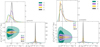 |
Fig. 15. As in Fig. 11, but for the derived variables that give the first two moments of the LF. |
| In the text | |
|
Fig. 16. Triplets of the Schechter function parameters (Φ*, L*, and α) that give exactly the same values of the first two moments as our pessimistic LF at z = 5 (solid) and 3.6 (dashed). |
| In the text | |
|
Fig. 17. Left: Marginalised posterior distributions of the LF parameters obtained by fitting the LIM PS (green), the number counts of the targeted ALPINE survey (orange), and the combination of the two datasets (violet). The shaded areas indicate the 68% and 95% credible regions. Right: As in the left panel, but for the fit of the combined datasets and for different LIM surveys. |
| In the text | |
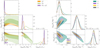 |
Fig. 18. As in Fig. 17, but for the pessimistic case with a faint-end slope of α = −1.9. |
| In the text | |
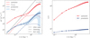 |
Fig. C.1. Same as Fig. 8 but for R = 500. |
| In the text | |
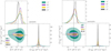 |
Fig. C.2. Same as Fig. 11, but for R = 500. |
| In the text | |
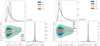 |
Fig. C.3. Same as Fig. 15, but for R = 500. |
| In the text | |
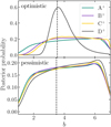 |
Fig. C.4. Same as Fig. 12, but for R = 500. |
| In the text | |
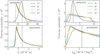 |
Fig. C.5. Same as Fig. 13, but for R = 500. |
| In the text | |
Current usage metrics show cumulative count of Article Views (full-text article views including HTML views, PDF and ePub downloads, according to the available data) and Abstracts Views on Vision4Press platform.
Data correspond to usage on the plateform after 2015. The current usage metrics is available 48-96 hours after online publication and is updated daily on week days.
Initial download of the metrics may take a while.