| Issue |
A&A
Volume 700, August 2025
|
|
|---|---|---|
| Article Number | A236 | |
| Number of page(s) | 17 | |
| Section | The Sun and the Heliosphere | |
| DOI | https://doi.org/10.1051/0004-6361/202555189 | |
| Published online | 26 August 2025 | |
Revisiting the hypothesis of purely stochastic excitation of global p modes in the Sun
1
Université Paris Cité, Université Paris-Saclay, CEA, CNRS, AIM, 91191 Gif-sur-Yvette, France
2
Université Paris-Saclay, Université Paris Cité, CEA, CNRS, AIM, 91191 Gif-sur-Yvette, France
3
INAF – Osservatorio Astrofisico di Catania, Via S. Sofia, 78, 95123 Catania, Italy
4
Instituto de Astrofísica de Canarias (IAC), 38205 La Laguna, Tenerife, Spain
5
Universidad de La Laguna (ULL), Departamento de Astrofísica, 38206 La Laguna, Tenerife, Spain
⋆ Corresponding author: This email address is being protected from spambots. You need JavaScript enabled to view it.
Received:
17
April
2025
Accepted:
30
June
2025
Abstract
Context. In solar-like oscillators, acoustic waves are excited by turbulent motion in the convective envelope and propagate inward, generating a variety of standing pressure modes (p modes). When combining the power of several solar acoustic modes, some studies have reported an excess that is not compatible with pure stochastic excitation. This excess could be a signature of a second mode excitation source.
Aims. With over 27 years of helioseismic data from the Sun-as-a-star observations by the Solar and Heliospheric Observatory (SoHO), we aim to study the variation in mode energy over this period, covering solar cycles 23 and 24, as well as the beginning of cycle 25. In particular, we focus on the possible sources of high peaks in the mode-energy time series, namely, instrumental problems, or other exciting mechanisms, such as flares or coronal mass ejections (CMEs).
Methods. We reconstructed the energy time series for each mode, resulting in 36 time series with a sampling time of 1.45 days. By combining the small timescale variations in energy for several low-degree modes (ℓ ≤ 2) in the 2090–3710 μHz range, we were able to study the correlation between the modes and their compatibility with the hypothesis that modes are only stochastically excited by convection.
Results. The observed excitation rate significantly deviates from what would be expected in the case of a purely stochastic excitation. Our results indicate that this energy excess cannot solely be attributed to instrumental effects and it does not exhibit a cyclic variation. Although high-energy excesses are occasionally associated with observations of flares and/or CMEs, no consistent pattern could be identified. The excitation is slightly more frequent for modes probing the upper layer of the convective zone. Furthermore, the energy supply rate seems to vary over time with the mean value following a modulation that can match the quasi-biennial oscillation (QBO) observed in other solar indicators, with the variance shown to be anti-correlated with the cycle.
Key words: methods: data analysis / Sun: activity / Sun: helioseismology / Sun: interior
© The Authors 2025
 Open Access article, published by EDP Sciences, under the terms of the Creative Commons Attribution License (https://creativecommons.org/licenses/by/4.0), which permits unrestricted use, distribution, and reproduction in any medium, provided the original work is properly cited.
This article is published in open access under the Subscribe to Open model. This email address is being protected from spambots. You need JavaScript enabled to view it. to support open access publication.
1. Introduction
Observations of stellar oscillations help set constraints on the internal properties of the stars. Variable stars are found across the entire Hertzsprung-Russell diagram (HRD) and various mechanisms are capable of exciting their pulsations, depending on their fundamental properties and structure (e.g. Christensen-Dalsgaard 2008; Aerts & Tkachenko 2024, and references therein).
Solar-like stars are composed of an internal radiative zone surrounded by an external convective envelope. In these stars, convection operates in a regime of fully developed turbulence, characterised by extremely high Reynolds numbers (Re ≫ 106). This turbulent flow transfers energy from large convective scales down to the small dissipative scales (Kolmogorov 1941). In this complex dynamical regime, the turbulent motions of the stellar plasma, along with fluctuations of thermodynamic quantities, randomly inject energy into the star’s oscillation eigenmode (in particular, the acoustic (or p) modes) through a mechanism known as stochastic excitation (e.g. Goldreich & Keeley 1977; Samadi & Goupil 2001; Belkacem et al. 2008). This process leads to the continuous excitation of several oscillation modes, which are simultaneously driven and damped (Belkacem et al. 2012). Both processes occur on different characteristic timescales (Samadi et al. 2015). Consequently, the power spectra of these modes exhibit Lorentzian profiles, with amplitudes that are determined by the balance between excitation and damping.
Moreover, solar-like stars also experience magnetic field variations, driven by a dynamo mechanism (Mathur et al. 2014). The solar magnetic field evolves following an 11-year cycle (Schwabe cycle) with a change in polarity at the end of each cycle. The modes frequency and amplitude variations in relation with the solar magnetic cycle has been extensively studied (e.g. García et al. 2013; Salabert et al. 2015), as well as modes parameter variations for magnetically active solar-like stars other than the Sun (e.g. Régulo et al. 2016; Santos et al. 2019). Frequencies increase with the magnetic field strength whereas amplitudes decrease. Bessila & Mathis (2024) derived the formalism describing the excitation of the p modes by convective motions in presence of a magnetic field, demonstrating that the mode amplitude decreases with the magnetic field strength. Furthermore, previous studies have measured a constant energy supply rate over time for low-degree modes, attributing this constancy to a balance between damping and excitation processes (Chaplin et al. 2000; Jiménez-Reyes et al. 2004). However, for the first time, Kiefer & Broomhall (2021) observed that the energy supply rate varies over the cycle for intermediate-degree modes (2 < ℓ < 150), with this variation being anti-correlated with the solar cycle. They further suggested that modes with frequencies below 3000 μHz are more strongly influenced by this variation, as well as modes with degrees greater than ℓ ∼ 20.
After having studied the correlation between modes energies with data from the InterPlanetary Helioseismology by IRradiance measurements (IPHIR, Fröhlich et al. 1988) and the first 310 days of data from the Global Oscillation at Low Frequencies (GOLF, Gabriel et al. 1995) of the Solar and Heliospheric Observatory (SoHO, Domingo et al. 1995), Baudin et al. (1996) and Foglizzo (1998, hereafter cited as F+98) found a correlation between several low-degree modes. In F+98, it was even noted that several modes were excited at the same time during the end of 1998. Because this is not expected if modes are only stochastically excited by convection, they suggested the existence of a second source of mode excitation. The possibility of high-energy flares, specifically X-class flares with a flux greater than 10−4 W m−2 and coronal mass ejections (CMEs) injecting energy into modes, has been investigated by Foglizzo (1998). The typical size of flares observed from the Earth is of the order of a few arcminutes, suggesting that they have the potential to excite over 104 modes. However, assuming an equal distribution of energy, their intensity is insufficient to supply the necessary energy for the excitation of each acoustic mode. Nevertheless, the typical latitude distance between the foot points of the outer loop of the CMEs is about 45 degrees. Considering this as the CME’s typical size, they should be able to excite less than a hundred low-degree modes. Based on an estimation of the CMEs’ kinetic energy, Foglizzo (1998) suggested that they may transfer sufficient energy to excite these modes. With more than 28 years of continuous observations from the Solar and Heliospheric Observatory (SoHO) available now, covering solar magnetic cycles 23, 24, and approximately the first half of cycle 25, the relationship between the energy of these modes and solar magnetic variations must be re-investigated, and compared to flare and CME occurrences.
The heliospheric data are described in Sect. 2 and the data processing to reconstruct an energy time series for each mode is described in Sect. 3. Section 4 explains our statistical analysis on the energy variation of the modes, which is discussed in Sect. 5.
2. Helioseismic time series
The Solar and Heliospheric Observatory (SoHO, Domingo et al. 1995) was launched in December 1995, with three onboard instruments for helioseismology: Michelson Doppler Imager (MDI, Scherrer et al. 1995) of the Solar Oscillation Imager (SOI), Global Oscillation at Low Frequencies (GOLF, Gabriel et al. 1995) spectrometer, and Variability of solar IRradiance and Gravity Oscillations (VIRGO, Fröhlich et al. 1995). Measurements of GOLF and VIRGO SunPhotoMeters (SPMs) are integrated over the solar disk and can therefore be compared with other stars observations. GOLF observes in its single wing configuration, namely, it measures mainly the blue wing of the sodium doublet at 589.6 and 589.0 nm since 11 April 1996, although it was switched to the red-wing configuration after the SoHO recovery mission on September 1998 to November 2002 (see García et al. 2005). From these measurements, a proxy of the Doppler velocity is produced as shown in Pallé et al. (1999). The cadence of the observations is 5 s, but the time series were then calibrated and resampled to multiples of 20 s. VIRGO/SPMs measures the sunlight irradiance integrated over the solar disk since 23 January 1996, with a 60 s cadence, in three wavelengths of the optical band: 402 nm (blue channel), 500 nm (green channel), and 862 nm (red channel). In this work, an asteroseismic proxy was built combining green and red channels from VIRGO/SPMs measurements, as this combination is the most similar to the Kepler passband (Basri et al. 2010), allowing for more straightforward comparisons with other stars. The calibration of these data is described in Appendix A.1. GOLF and VIRGO/SPMs measurements cover a period from the minimum between solar magnetic cycles 22 and 23 to the ongoing maximum of cycle 25.
3. Data processing: Temporal evolution of a single mode
The observed time series depend on many contributions such as rotation, granulation, solar activity, oscillation modes, and photon noise; with each of them having a contribution at a distinctive frequency range. The energy contribution from a mode can be isolated and extracted, following the procedure first described by F+98. By isolating the contribution of each mode by filtering in the Fourier domain and computing its inverse Fourier transform, we can reconstruct its energy time series. Following the analogy with a simple harmonic oscillator of eigenfrequency ω0, F+98 showed that the surface energy per unit of mass εn, ℓ of a mode can be approximated by:
 (1)
(1)
where fv(t) is the inverse Fourier transform of the oscillatory velocity and M is the mode mass. If  is the single mode-filtered Fourier transform of the original time series, according to the window of size Δω, fv(t) can be expressed as
 (2)
(2)
The steps of the reconstruction method are summarised as follows:
-
Computation of the Fourier transform of the time series;
-
Selection of the central frequency of a mode in the Fourier domain according to the Δω window centred on the central mode frequency. The filtering is performed by setting all frequencies outside this window to zero. In Fig. 1, the PSD of p modes between 2400 μHz and 2900 μHz from GOLF observations is shown. Two windows of 8 μHz, centred on the middle frequency of the modes (n = 24, ℓ = 2) and (n = 25, ℓ = 0) are illustrated;
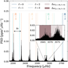
Fig. 1. PSD of the VIRGO/SPMs light curve (from 23.01.1996 to 23.11.2023). Higher frequencies are displayed between 3270 and 3750 μHz, showing the large frequency separation (δν) noted between modes ℓ = 0 and ℓ = 1 for n = 23. Modes are marked by vertical lines with different colours: n = 22 in light blue, n = 23 in orange, n = 24 in yellow, n = 25 in cyan, and n = 26 in dark blue). ℓ = 0 are in continuous, ℓ = 1 in dashed, ℓ = 2 in dotted, and ℓ = 3 in dot-dashed lines. In the subplot: Window of Δω = 8 μHz used to reconstruct modes energy time series is shown around modes (n = 25, ℓ = 0) in light brown and (n = 24, ℓ = 2) in dark brown.
-
Translation of the window towards central frequency ω0 = 0;
-
Computation of the inverse Fourier transform of it according to Eq. (2);
-
The energy time series of the mode εn, ℓ(t) is given by Eq. (1).
To validate our implementation, we applied this process to a half-day period simulated signal of a quasi-periodic oscillation with three random excitations. Results of the reconstruction with a window of 40 μHz are displayed in Fig. 2 for a time series of 10 days sampled at 60 seconds. Period scales of this simulated signal were deliberately chosen as different from what is expected from the modes for more readability. Comparing ε(t) with the reconstructed energy clearly demonstrates that this method retrieves the envelope of the energy time series, which is essential for determining the excitation times. We validated that it respects Parseval’s theorem, comparing the integrals of the squares of the filtered signal in both the Fourier domain and the time domain. In Fig. 2, the time resolution difference we get between the original signal and the reconstructed one is also shown. As discussed by F+98, the time resolution δt of the energy time series is related to the size of the Δω filtering window,
 (3)
(3)
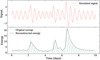 |
Fig. 2. Top panel: Simulated sinusoidal signal S(t) with a period of 0.5 days and three excitations randomly distributed in time. It is shown for a time series of 10 days sampled at 60 seconds. The excitations are exponentially decaying. Bottom panel: Energy E(t) = 2|S(t)|2 corresponding to the simulated signal is shown in grey and the reconstructed energy is shown in dashed black. |
It sets a limit of binning for the reconstructed signal, ruled by both the window size and the resolution in the Fourier domain 1/T, where T is the total observation length: the number of points in the reconstructed signal is p = T Δω. The larger the window size the better the resulting resolution of the reconstructed time series. Moreover, Δω should be large enough to include the total power of the mode peak but small enough for windows around nearby modes not to overlap each other. For example, a maximum window of 8 μHz is illustrated on Fig. 1 around high frequencies modes (n = 25, ℓ = 0) and (n = 24, ℓ = 2). As the modes at higher frequencies are broader, it could be harder to set a window size for their reconstruction. However, in this case, it is possible to reconstruct the energy time series of several successive modes at a time (e.g. ℓ = 0 and ℓ = 2 or ℓ = 1 and ℓ = 3 modes), keeping in mind that several modes contributed to the resulting time series. For the solar case, the time series are sufficiently resolved in the frequency domain, allowing us to consider one mode at a time.
4. Analysis of the energy time series
We begin this section by describing the reconstruction of mode energy for the VIRGO/SPMs data. Subsequently, we present the statistical tests we used to evaluate the stochastic and non-stochastic behaviour of the mode energy.
4.1. Reconstruction of the VIRGO/SPMs energy time series
All n = 14 to n = 25 and ℓ = 0 to ℓ = 2 modes were reconstructed using a window Δω = 8 μHz, as recommended by F+98 and illustrated in Fig. 1. The reconstructed time series, with a time resolution of δt ∼ 1.45,days, allows for the study of short-term variations for each mode, in contrast to other classical methods. The window is centred on the mode frequencies listed in Lazrek et al. (1997), originally derived from early GOLF data via peakbagging and also valid for VIRGO/SPMs observations (Toutain et al. 1997). Even though the frequencies of some ℓ = 3 to ℓ = 5 modes were constrained by Lazrek et al. (1997), we chose not to include them in this study due to their low signal-to-noise ratio (S/N). Moreover, since their frequencies are not within Δω of the ℓ = 0 to ℓ = 2 modes, they do not impact our reconstruction. For comparison between modes, each time series was normalised by its mean. Figure 3 illustrates the normalised energy for n = 22, ℓ = 0 during solar cycle 24 and as expected, the excitation looks stochastic during this epoch.
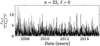 |
Fig. 3. Normalised reconstructed energy time series for n = 22, ℓ = 0, with VIRGO/SPMs data. For better visibility, we restricted the x-axis between 2007 and 2015. The series were reconstructed from 23 January1996 to 17 February 2016. |
4.2. Statistical tests on complete energy time series
Under the hypothesis of stochastically excited modes by convection and neglecting the mode asymmetry, each resulting time series should be distributed according to a theoretical exponential distribution, fth, defined by its mean λ for positive values of x:
 (4)
(4)
and this is confirmed by Eq. (1) assuming that the distribution of oscillatory velocities is Gaussian.
We performed Kolmogorov-Smirnov (KS) tests to compare for each mode, the agreement between the reconstructed time series and fth. This statistical test compares a sample to a theoretical distribution (Massey 1951) by evaluating several statistics including the maximum distance between both cumulative distributions and the p-value. The null hypothesis, H0, is that the observed distribution follows the theoretical one. In this context, the p-value estimates the probability of being wrong in rejecting H0. As is commonly done, we set a 5% threshold for the p-value in order to choose whether or not to reject H0. All the statistical tests were conducted while excluding values associated with gaps longer than one day in the original time series. Additionally, a data point at the edges before and after these gaps were removed to prevent potential edge effects during the reconstruction. The dates of these gaps are listed in Table 1. The values for λ were estimated via maximum likelihood estimation (MLE) from the 6858 points of each dataset, by minimising the negative log-likelihood function, defined as
Starting and ending dates of the gaps greater than one day in the VIRGO/SPMs data.
 (5)
(5)
where n is the total number of observations and xi are the observed data points. The resulting p-values of the KS tests are shown in Fig. 4 as well as the rejection threshold of 5%. None of the points are below this threshold: all distributions correspond to modes that are not incompatible with exponential distributions according to the test.
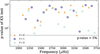 |
Fig. 4. Resulting p-values of the Kolmogorov-Smirnov tests comparing reconstructed time series distributions with exponential distributions. Orange triangles stand for ℓ = 0 modes, dark blue squares for ℓ = 1 modes, and light blue circles for ℓ = 2 modes. The threshold of rejection of 5% is drawn as a dashed black line. |
4.3. Statistical tests on activity-dependent subsamples
Thresholds and used to define starting and ending dates of each cycle extremum for cycles 23, 24, and 25.
Given that the mode parameters are affected by solar activity, we repeated the statistical analysis of the mode energy using sub-samples corresponding to low and high levels of magnetic activity. Among the various activity proxies discussed in Jain et al. (2009), the solar radio flux index, F10.7 (Tapping 2013), sensitive to the upper chromosphere, shows the strongest correlation with p-mode frequency shifts over full solar cycles. Based on these findings, F10.7 is selected as our reference proxy to define epochs of low and high activity (see Appendix B). Table 2 summarises the corresponding dates for solar minima and maxima.
Each reconstructed time series was divided into two subsets: one for low activity (1735 points) and one for high activity (2125 points). The KS tests were then performed separately to each and figure 5 shows the resulting p-values. Three p-values fall below the 5% threshold, all corresponding to high-activity intervals. Given that 72 tests were conducted, observing a few rejections is statistically expected. However, the fact that all rejections occur during high activity periods suggests a possible, though subtle, deviation from the stochastic model during these phases.
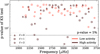 |
Fig. 5. Resulting p-values of the Kolmogorov-Smirnov tests comparing reconstructed time series distributions with exponential distributions, for measurements taken during low and high magnetic activity periods whose dates are listed in Table 2. Triangles stand for ℓ = 0 modes, squares for ℓ = 1 modes, and circles for ℓ = 2 modes. Brown and pink makers stand for tests on values taken during high (resp. low) magnetic activity. The threshold of rejection of 5% is drawn as a dashed black line. |
4.4. Statistical study of non-stochasticity in the modes excitation
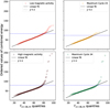 |
Fig. 6. Q-Q plot comparing the combined energy time series with |

To explore potential deviations from purely stochastic excitation, we combined all 36 normalised mode energy time series into a single sequence. Under the hypothesis of independent, exponentially distributed signals, the resulting distribution should follow a Gamma-distribution of order k, corresponding to the number of combined modes. Further KS tests were performed for four subsets of the sequence: low and high activity, both already considered in Sect. 4.3, and the maxima of cycles 23 and 24, separately. We considered the parametrised Gamma-distribution noted  , defined by:
 (6)
(6)
where Γ(x) denotes the Euler Gamma function, while α and β are, respectively, the location and the scale parameters. Fixing k = 36, α and β parameters were fitted via MLE by minimizing:
![Mathematical equation: $$ \begin{aligned} \log L(k = 36, \alpha , \beta )&= n[k\log \beta -\log \Gamma (k)] \nonumber \end{aligned} $$](/articles/aa/full_html/2025/08/aa55189-25/aa55189-25-eq10.gif) (7)
(7)
Fitted values for α and β are listed in Table 3 along with the resulting p-values of the KS tests.
List of α and β parameters along with resulting p-values of the performed KS tests.
Results statistically consistent with H0 are obtained only for the low-activity phase and the maximum of cycle 23 subsets. The p-value for cycle 23 is indeed close to 50%, whereas for cycle 24, it is below the 5% threshold. The constrained estimates of the parameters α and β indicate a clear divergence in mode energy distributions between low- and high-activity subsets, as well as between the maxima of cycles 23 and 24. This discrepancy is also evident in the quantile-quantile (Q-Q) plots presented in Fig. 6, where data points above the 98% quantile systematically deviate from the theoretical distributions, especially in subsets with lower KS test p-values. The deviations from the y = x reference line are more pronounced for high-activity phases, compared to low-activity ones; for the maximum of cycle 24 relative to the maximum of cycle 23. These findings suggest that the statistical properties of mode energy during periods of high-magnetic activity are significantly influenced by the distinct behaviour of cycle 24 and that there is a difference between the maximum of cycle 23 and that of cycle 24, corroborating previous results reported by, for instance, García et al. (2024). Figure 7 shows the corresponding Gamma-distributions. As expected from the anti-correlation between mode energy and magnetic activity, the mean combined energy is higher during low-activity periods than during high-activity ones. The mean normalised energy is also lower during the maximum of cycle 23 than that of cycle 24, again highlighting differences between the two cycles. Moreover, variance likewise varies with activity: it is smaller during the cycle 23 maximum compared to low activity, but greater during the cycle 24 maximum.
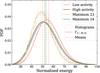 |
Fig. 7. Distributions of normalised combined energies. For each cycle period, we show the histogram, the best |

To quantify the high-energy excess seen in Fig. 6, we analysed short-timescale fluctuations in energy by dividing the combined time series by its one-year moving mean. This residual energy time series is further noted as 𝒮phot. The high-energy excesses are defined as the local maxima in 𝒮phot that have energies exceeding the threshold of xphot = 24.75, which corresponds to the 98% quantile of 𝒮phot. The best-fit Gamma distribution for 𝒮phot yields αphot = −58.05, ±0.49 and βphot = 1.59, ±0.02, with a p-value of 1.63 × 10⁻³, %, indicating a strong deviation from the theoretical model. After removing peaks above the threshold, the p-value rises to 30.15%, confirming that high-energy events are the source of the deviation. The expected probability of observing events above the given threshold x can be estimated by applying the binomial probability formula,
 (8)
(8)
with r = 108, n = 6612 and  . We find P ≪ 10−3, where the observed number of high-energy events is significantly higher than expected from a stochastic model. Our results echo previous studies by Chaplin et al. (1997), Chang & Gough (1998), who found a power excess in the modes when working with a total of ∼763.8 days of the Birmingham Solar-Oscillations Network (BiSON) data, collected in short segments of 11.4 h. We further discuss the found excess of energy in Sect. 5.
Now focusing on the energy below the threshold xphot (statistically consistent with a stochastic excitation), we can compute the energy supply rate ( , e.g. Jiménez-Reyes et al. 2003). The central finite difference formula giving a second-order approximation of the elements i of the first derivative of a function f(x), can be adapted to discrete functions with a non-constant step size with:
 (9)
(9)
where f(x) is supposed three times differentiable, hi = xi + 1 − xi and hi − 1 = xi − xi − 1 (Quarteroni et al. 2007). The temporal mean and variance of Ė were computed over one-year sub-series, shifted every eighth of a year. The results are illustrated in Fig. 8. The variation in the mean energy supply rate follows a quasi-biennial oscillation (QBO) pattern, consistent with previous findings in mode frequency shifts and magnetic proxies (Bazilevskaya et al. 2014, and references therein). The variance is anti-correlated with solar activity and shows stronger fluctuations during cycle 24 than cycle 23, in agreement with similar observations from high-degree mode analyses using GONG data (Kiefer & Broomhall 2021).
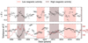 |
Fig. 8. Mean (top panel) and variance (bottom panel) of a one-year subseries slided every eighth of a year of the energy supply rate computed from the combined time series of the modes. These quantities are plotted against the central date of the considered subseries and the x-axis error bars show the range of dates taken for each subseries. Periods of low (pink) and high (brown) magnetic activity are reported from Table 2 and |

5. Possible explanations for energy excess
The time series of the combined energy of the modes reveals an excess of energy in the modes compared to the expected level under the hypothesis of stochastic excitation by turbulent convection. To better understand this discrepancy, several potential sources were investigated. Here, we analyse the temporal correlation of the 108 high-energy points with a set of indicators: the occurrence of energetic flares and CMEs, the reconstructed mode energy from GOLF observations, and the potential influence of either photon noise in the VIRGO/SPM instruments or convective processes. Analysing the sensitivity depth of the modes, the possible location of their non-stochastic excitation is also discussed. After detailing the data used in Sect. 5.1 for which the notations are summarised in Table 4, we explore the potential sources of high-energy peaks found in 𝒮phot in Sect. 5.2.
Summary of the notations introduced for the discussed time series.
5.1. Complementary indicators
5.1.1. Contribution from other frequency scales
Since the reconstruction is sensitive to the photon noise level, we applied the same reconstruction procedure, using the mode pattern shifted to higher frequencies, namely, adding 4500 μHz to each mode’s central frequency. This yielded 36 windows of 8 μHz between 6590 and 8210 μHz. Each time series was normalised by the mean energy of the corresponding mode in 𝒮phot, and the resulting 36 series were combined into a new time series, σphot, where 92 points exceed the 98% quantile threshold.
An analogous reconstruction was performed with a downward shift of 2000 μHz, yielding an energy time series dominated by convective contributions, denoted as 𝒞phot, where 103 points lie above the threshold.
5.1.2. Flares and CMEs
Flares are classified based on their peak X-ray flux in the 1–8 Å range. X-class flares (with a flux greater than 10−4 W m−2) correspond to energy releases larger than 1032 ergs, and were extracted from data of the Geostationary Operational Environmental Satellite1 (GOES, Mallette 1982). In the same way, the top 5% most energetic CMEs (with an energy greater than 1.3 × 1031 ergs) were selected from measurements taken by the Large Angle and Spectrometric COronagraph experiment2 (LASCO, Brueckner et al. 1995) aboard SoHO. Over the VIRGO/SPMs operational period, 1271 CMEs and 195 X-class flares were recorded.
5.1.3. Mode energy time series from GOLF data
The energy time series for the same modes were reconstructed from GOLF data starting on 18 November 2002, when the instrument was switched back to its blue-wing configuration. These series were normalised by their 365-day moving mean to correct for the annual modulation in photon noise (see Appendix A.1 and García et al. 2005). Spearman’s rank correlations were then computed between 𝒮phot and the GOLF time series, as shown in Fig. 9. With a rejection threshold at 5%, all modes except n = 14, ℓ = 2 were significantly correlated. The correlation strength increases with the power of the mode, and therefore with its S/N. This discrepancy between the datasets is consistent as the convective background is higher in VIRGO/SPMS than in GOLF, resulting in different amplitudes of the power spectral density (PSD), particularly for the lower frequency modes. The combined time series from GOLF, denoted 𝒮vel, exhibits 76 peaks above the 98% quantile.
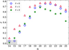 |
Fig. 9. Spearman’s rank correlation ρ between 𝒮phot and 𝒮vel data, versus radial order n for all considered modes. Blue circles stands for ℓ = 0 modes, red triangles for ℓ = 1, and green stars for ℓ = 2. Markers in the grey area correspond to a p-value larger than 10−3%. |
5.1.4. Combined time series in three frequency bands
Because acoustic modes are sensitive to different regions of the star depending on their frequency, we grouped the reconstructed modes into three frequency bands: 2090–2620 μHz, 2620–3160 μHz, and 3160–3710 μHz, each containing 12 modes, respectively denoted ℒphot, ℳphot, and ℋphot, when filtered by their one-year moving mean. The computation of the mean sound-speed kernels, ⟨𝒦⟩, which indicate the depth of maximum sensitivity for each band, is described in Appendix C. The estimated depths of maximum sensitivity are 1895 km for ℋphot, 1014 km for ℳphot, and 605 km for ℒphot beneath the surface.
The KS tests were performed comparing each band’s time series to theoretical Gamma-distributions for the same subsets described in Sect. 4.4. Table 5 summarises the resulting p-values and the estimated α and β parameters, this time fixing k = 12 in Eq. (6). A similar pattern to that observed in the total time series is found across all frequency bands, with smaller p-values during the maximum of cycle 24 than during the maximum of cycle 23. Notably, in the low-frequency band, the p-value drops below the 5% threshold during periods of high magnetic activity. In contrast, the high-frequency band shows a higher p-value during high activity than during low activity, whereas the opposite behaviour is seen in the two lower-frequency bands. Peaks exceeding the 98% quantile were identified for the three time series, yielding 121, 115, and 123 peaks in the low-, medium-, and high-frequency bands, respectively. Their temporal distribution is shown in Fig. 10. The number of high energy peaks in the medium-frequency band notably exhibit an anti-correlation with the solar cycle, suggesting a possible excitation mechanism linked to solar activity. This anti-correlation is absent in the other two bands, a difference possibly related to their lower S/N.
Resulting p-values of the KS tests performed to compare combined energy time series in the three frequency bands 2090–2620 μHz, 2620–3160 μHz, and 3160–3710 μHz, with the best  distributions.
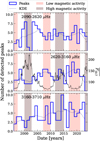 |
Fig. 10. Distribution of the detected peaks over time for the three frequency bands, from top to bottom: 2090–2620 μHz, 2620–3160 μHz, and 3160–3710 μHz. Each bin corresponds to one year from 1995 to 2025. Dashed curve shows the Epanechnikov kernel density estimations (KDE) of the probability distributions from each histogram. Periods of low and high magnetic activity were reported from Table 2 and |

5.2. Analysis and discussion
We now examine potential sources behind the observed high-energy excess in the modes. The key values in this section are illustrated in Fig. 11 and listed in Appendix D.
5.2.1. External sources affecting the measurements
The calibration of the VIRGO/SPMs and GOLF data includes sigma-clipping to remove outliers, such as flare and CME contributions (García et al. 2005). However, uncorrected external events (e.g. particle hits) would elevate the photon noise across all frequencies. Of the 108 high-energy peaks in 𝒮phot, 26 coincide within δt = 1.45 days with a peaks in σphot. Additionally, 34 peaks occurred simultaneously (within a window of δt = 1.45 day), with at least one CME, and 14 with at least one X-class flare. For example, Fig. 11 shows that an X-class flare coincided with an energetic peak in 𝒮phot in early 2004. However, no correlation was found between the energy associated with the event and the occurrence of a mode energy peak. Among the 34 CME-related peaks, 11 are also present in σphot, as are 5 of the 14 flare-related peaks. In total, 13 peaks could be attributed to both flares and/or CMEs affecting the measurements and the 13 other peaks correlating σphot could be attributed to another external source.
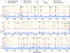 |
Fig. 11. 𝒮phot is shown in light blue in the lower part of each panel, along with the detected high-energy peaks marked by dark blue crosses. For better clarity, the full 27-year time series is divided into three panels (from top to bottom). For each peak, when it corresponds to a peak in σphot (resp. in 𝒞phot or in 𝒮vel), within a window of δt = 1.45 days, a red (resp. pink or brown) circle highlights it in the top light beige area of each panel. Similarly, when at least one X-class flare (or one CME) occurred within the δt-window around the peak, it is marked by an orange (or green) circle. Peaks not coinciding with any of these events are marked by violet circles. Furthermore, if a peak is detected within one of the three defined frequency bands, it is highlighted with a black marker: a square for low frequencies, a star for medium frequencies, and a triangle for high frequencies. Gaps due to the SoHO recovery mission are represented as grey shaded areas. Minor ticks represent months. |
5.2.2. Flares and CMEs being able to excite p modes
To test whether flares or CMEs could actively excite modes, we examined coincidences between VIRGO/SPMs and GOLF high-energy peaks, from 26 May 2003 to 3 May 2022. Of the 76 peaks in 𝒮vel, 12 coincided with 𝒮phot. Since both instruments are located on the same satellite, the presence of common high-energy excesses can be attributed to either instrumental factors or the modes themselves. However, only two of these also aligned with σphot and known flare and CME events, suggesting an external instrumental origin. The remaining ten shared peaks likely reflect genuine mode behaviour. Only one aligns with a CME and one with a flare, suggesting a lack of systematic correlation. The mode amplitudes vary according to both the instrument. Moreover, this study does not account for the reversal of mode asymmetry observed between intensity and velocity spectra (Toutain et al. 1997, 1998; Nigam & Kosovichev 1998; Chaplin & Appourchaux 1999) and the influence of a correlated noise in GOLF data (Thiery et al. 2001). In particular, Fig. 9 suggests that if lower-frequency modes are excited simultaneously, the low correlation between instruments could lead to a high-energy peak being detected by one instrument but missed by the other. Between 2005 and 2009, all peaks detected exclusively in 𝒮vel correspond to modes in the medium or high-frequency bands, while during the same period, none of the high-energy peaks from the low-frequency band were detected. This observation aligns with the reduced correlation between VIRGO/SPMs and GOLF data for low-frequency modes. Furthermore, none of the ten peaks correlated with 𝒞phot but not with σphot show correlation with 𝒮vel. Given that the convective power level is higher in VIRGO/SPMs data compared to GOLF, these findings reinforce the hypothesis that convection contributes to some of the high-energy peaks observed in 𝒮phot.
Moreover, assuming that flares and CMEs originate only at or near the solar surface, and not within the deeper solar interior, one might expect that if these events were capable of exciting the modes, higher-frequency modes would be preferentially excited before lower-frequency ones. To investigate this, we examined the 82 peaks in 𝒮phot that show no correlation with σphot. Among these, 23 coincide with CMEs, with 6, 9, and 6 peaks occurring in the low-, medium-, and high-frequency bands, respectively. Similarly, of the 9 peaks associated with X-class flares, 4, 2, and 3 are found in ℒphot, ℳphot, and ℋphot. These distributions indicate that excitation signatures are approximately uniform across frequency bands, inconsistent with a surface-limited excitation mechanism.
Consequently, the hypothesis that these surface events act as a secondary excitation mechanism appears unsupported. This conclusion aligns with the theoretical analysis of Foglizzo (1998), which argued that flares lack the energy, relative to their spatial extent, to efficiently excite individual modes. Although CME-driven excitation presents a marginally more plausible case, it still depends on assumptions about their spatial scale, inferred from the separation of loop footpoints. Given that flares and CMEs are likely manifestations of the same underlying process, and considering CME onset estimates from Yashiro & Gopalswamy (2009), a smaller initiation scale is plausible. In that scenario, the available kinetic energy of CMEs would also be insufficient for effective mode excitation.
5.2.3. Locating the mode excitation
Of the 82 peaks in 𝒮phot not associated with σphot, 44 show no correlation with any of the studied proxies and 12 are correlated only with peaks in 𝒮vel. When divided into frequency bands, 20, 23, and 28 of these peaks fall into the low-, medium-, and high-frequency ranges, respectively. Only one peak (observed in December 2012) was detected across all three frequency bands, but not in 𝒮vel. The slight excess of high-frequency events suggests a possible excitation source located in the outermost layers of the convective zone. Meanwhile, exciting modes simultaneously in the low- and high-frequency bands, but not in the medium one, occurs four times during the total observation period of VIRGO/SPMs. This suggests the presence of a mechanism that primarily acts at the edges of the region where the modes are the most sensitive, rather in the middle layers. The temporal variations (shown in Fig. 10) further support the existence of an intricate, time-dependent excitation mechanism, with spatial and temporal characteristics that evolve over the solar cycle. Furthermore, this exciting mechanism is expected to have a timescale that is smaller or at least similar to the five-minute timescale of the modes (details in Appendix E).
6. Conclusions
In this study, we analyse over 27 years of data from the SoHO VIRGO/SPMs and GOLF instruments using the methodology developed in F+98 to reconstruct the energy time series of low-degree modes (ℓ ≤ 2). For each mode with a radial order of 14 ≤ n ≤ 25, we compared the observed energy distribution to the expected distribution under the assumption that the modes are only stochastically excited by convection. The general behaviour of the modes is found to be consistent with stochastic excitation. However, similarly to previous studies (Chaplin et al. 1997; Chang & Gough 1998), we observed that the modes are excited at an unusually high rate, indicating non-stochastic characteristics in the excitation mechanisms. On the one hand, we computed a proxy for the energy supply rate, which appears to fluctuate over time. The mean < Ė > follows a quasi-biennial oscillation (QBO) pattern and its variance appears to be anti-correlated with the solar cycle. On the other hand, we made a temporal comparison of the occurrence of these high-energy peaks with the presence of energy sources, such as X-class flares or highly energetic CMEs. Although some high-energy points coincide with these events, there is no direct correlation between the energy released by the event and the occurrence of an energy excess, nor is there a systematic pattern of such events throughout the entire study period. By introducing a combination of modes within the frequency bands, we aimed to determine the location of the excitation process. Our results suggest the existence of a complex excitation mechanism that has the capacity to excite several modes at once and where the excitation region changes over time.
This study does not account for potential deviations from the energy distribution model described by Eq. (4) that could arise due to mode asymmetry. Addressing this limitation represents a natural follow-up, potentially through the development of a more comprehensive model that incorporates asymmetric mode profiles. Further extensions could also involve applying the same reconstruction method to higher degree modes to investigate whether similar correlations exist. This could be feasible using spatially resolved observations, such as those provided by SOI/MDI. Additionally, analogous analyses of mode excitation rates and energy in other solar-like stars would help characterize how energy excess is correlated with stellar magnetic activity and its temporal modulation.
Acknowledgments
The authors want to acknowledge Leila Bessila, Adam Finley, Kiran Jain, Barbara Perri and Antoine Strugarek for useful comments and discussions. The GOLF, VIRGO/SPMs and LASCO instruments on board SoHO are a cooperative effort of many individuals to whom we are indebted. SoHO is a project of international collaboration between ESA and NASA. The authors strongly acknowledge the French space agency, CNES, for its support to GOLF since the launch of SoHO. E.P. and R.A.G. acknowledge the support from the GOLF/SoHO and PLATO Centre National D’Études Spatiales grants. S.N.B acknowledges support from PLATO ASI-INAF agreement no. 2022-28-HH.0 “PLATO Fase D”. The authors want to thank the whole Kepler team, all funding councils and agencies that have supported the activities of the KASC and the International Space Science Institute. Funding for the Kepler mission is provided by NASA’s Science Mission. We thank the NOAA National Geophysical Data Center’s (NGDC) for making their data of the GOES solar flare X-ray freely available in the Solar Data Repository, accessible at ftp://ftp.ngdc.noaa.gov/STP/space-weather/solar-data/solar-features/solar-flares/x-rays/goes/. We also acknowledge Christensen-Dalsgaard et al. (1996) for publicly sharing their solar structure model accessible at https://users-phys.au.dk/jcd/solar_models/. Softwares: AstroPy (Astropy Collaboration 2013, 2018), Matplotlib (Hunter 2007), NumPy (van der Walt et al. 2011), SciPy (Jones et al. 2001), pandas (McKinney 2010; The pandas development team 2024) and GYRE (Townsend & Teitler 2013). Some portions of the text were revised with the help of OpenAI’s ChatGPT (GPT-4), used for improving clarity and scientific language.
References
- Aerts, C., & Tkachenko, A. 2024, A&A, 692, R1 [NASA ADS] [CrossRef] [EDP Sciences] [Google Scholar]
- Astropy Collaboration (Robitaille, T. P., et al.) 2013, A&A, 558, A33 [NASA ADS] [CrossRef] [EDP Sciences] [Google Scholar]
- Astropy Collaboration (Price-Whelan, A. M., et al.) 2018, ApJ, 156, 123 [CrossRef] [Google Scholar]
- Bahcall, J. N., & Serenelli, A. M. 2005, ApJ, 626, 530 [NASA ADS] [CrossRef] [Google Scholar]
- Basri, G., Walkowicz, L. M., Batalha, N., et al. 2010, ApJ, 713, L155 [Google Scholar]
- Basu, S., Broomhall, A.-M., Chaplin, W. J., & Elsworth, Y. 2012, ApJ, 758, 43 [NASA ADS] [CrossRef] [Google Scholar]
- Baudin, F., Gabriel, A., Gibert, D., Palle, P. L., & Regulo, C. 1996, A&A, 311, 1024 [NASA ADS] [Google Scholar]
- Bazilevskaya, G., Broomhall, A.-M., Elsworth, Y., & Nakariakov, V. M. 2014, Space Sci. Rev., 186, 359 [CrossRef] [Google Scholar]
- Belkacem, K., Samadi, R., Goupil, M. J., & Dupret, M. A. 2008, A&A, 478, 163 [NASA ADS] [CrossRef] [EDP Sciences] [Google Scholar]
- Belkacem, K., Dupret, M. A., Baudin, F., et al. 2012, A&A, 540, L7 [NASA ADS] [CrossRef] [EDP Sciences] [Google Scholar]
- Bessila, L., & Mathis, S. 2024, A&A, 690, A270 [NASA ADS] [CrossRef] [EDP Sciences] [Google Scholar]
- Brueckner, G. E., Howard, R. A., Koomen, M. J., et al. 1995, Sol. Phys., 162, 357 [NASA ADS] [CrossRef] [Google Scholar]
- Chang, H. Y., & Gough, D. O. 1998, Sol. Phys., 181, 251 [Google Scholar]
- Chaplin, W. J., & Appourchaux, T. 1999, MNRAS, 309, 761 [NASA ADS] [CrossRef] [Google Scholar]
- Chaplin, W. J., Elsworth, Y., Howe, R., et al. 1997, A&AS, 125, 195 [NASA ADS] [CrossRef] [EDP Sciences] [Google Scholar]
- Chaplin, W. J., Elsworth, Y., Isaak, G. R., Miller, B. A., & New, R. 2000, MNRAS, 313, 32 [CrossRef] [Google Scholar]
- Christensen-Dalsgaard, J. 2008, Lecture Notes on Stellar Oscillations, 5th edn. (Institut for Fysik og Astronomi, Aarhus Universitet) [Google Scholar]
- Christensen-Dalsgaard, J., Dappen, W., Ajukov, S. V., et al. 1996, Science, 272, 1286 [Google Scholar]
- Domingo, V., Fleck, B., & Poland, A. I. 1995, Sol. Phys., 162, 1 [Google Scholar]
- Elad, M., Starck, J. L., Querre, P., & Donoho, D. L. 2005, ACHA, 19, 340 [Google Scholar]
- Foglizzo, T. 1998, A&A, 339, 261 [NASA ADS] [Google Scholar]
- Fröhlich, C., Bonnet, R. M., Bruns, A. V., et al. 1988, in ESA, Seismology of the Sun and Sun-Like Stars, 286, 359 [Google Scholar]
- Fröhlich, C., Romero, J., Roth, H., et al. 1995, Sol. Phys., 162, 101 [Google Scholar]
- Gabriel, A. H., Grec, G., Charra, J., et al. 1995, Sol. Phys., 162, 61 [Google Scholar]
- García, R. A., & Ballot, J. 2019, Liv. Rev. Sol. Phys., 16, 4 [Google Scholar]
- García, R. A., Turck-Chièze, S., Boumier, P., et al. 2005, A&A, 442, 385 [NASA ADS] [CrossRef] [EDP Sciences] [Google Scholar]
- García, R. A., Salabert, D., Mathur, S., et al. 2013, J. Phys.: Conf. Ser., 440, 012020 [Google Scholar]
- García, R. A., Mathur, S., Pires, S., et al. 2014, A&A, 568, A10 [Google Scholar]
- García, R. A., Breton, S. N., Salabert, D., et al. 2024, A&A, 691, L20 [NASA ADS] [CrossRef] [EDP Sciences] [Google Scholar]
- Goldreich, P., & Keeley, D. A. 1977, ApJ, 211, 934 [NASA ADS] [CrossRef] [Google Scholar]
- Gough, D., & Thompson, M. 1991, Sol. Interior Atmosp., 1, 519 [Google Scholar]
- Hunter, J. D. 2007, CiSE, 9, 90 [Google Scholar]
- Jain, K., Tripathy, S. C., & Hill, F. 2009, ApJ, 695, 1567 [NASA ADS] [CrossRef] [Google Scholar]
- Jiménez, A., Roca Cortés, T., & Jiménez-Reyes, S. J. 2002, Sol. Phys., 209, 247 [CrossRef] [Google Scholar]
- Jiménez-Reyes, S. J., García, R. A., Jiménez, A., & Chaplin, W. J. 2003, ApJ, 595, 446 [CrossRef] [Google Scholar]
- Jiménez-Reyes, S. J., Chaplin, W. J., Elsworth, Y., & García, R. A. 2004, ApJ, 604, 969 [CrossRef] [Google Scholar]
- Jones, E., Oliphant, T., & Peterson, P. 2001, SciPy: Open source scientific tools for Python, http://www.scipy.org/ [Google Scholar]
- Kiefer, R., & Broomhall, A.-M. 2021, MNRAS, 500, 3095 [Google Scholar]
- Kolmogorov, A. 1941, Dokl. Akad. Nauk SSSR, 30, 301 [NASA ADS] [Google Scholar]
- Lazrek, M., Baudin, F., Bertello, L., et al. 1997, Sol. Phys., 175, 227 [NASA ADS] [CrossRef] [Google Scholar]
- Mallette, L. 1982, Geostationary Operational Environmental Satellite/GOES/ - A Multifunctional Satellite, 9th Communications Satellite Systems Conference [Google Scholar]
- Massey, F. J. 1951, J. Amer. Statist. Assoc., 46, 68 [Google Scholar]
- Mathur, S., García, R. A., Ballot, J., et al. 2014, Proc. IAU Symp., 302, 222 [Google Scholar]
- McKinney, W. 2010, scipy, https://doi.org/10.25080/Majora-92bf1922-00a [Google Scholar]
- Nigam, R., & Kosovichev, A. G. 1998, ApJ, 505, L51 [NASA ADS] [CrossRef] [Google Scholar]
- Pallé, P. L., Régulo, C., Roca Cortés, T., et al. 1999, A&A, 341, 625 [Google Scholar]
- Pires, S., Mathur, S., García, R. A., et al. 2015, A&A, 574, A18 [NASA ADS] [CrossRef] [EDP Sciences] [Google Scholar]
- Quarteroni, A., Sacco, R., & Saleri, F. 2007, Numerical Mathematics (Springer), 37 [Google Scholar]
- Régulo, C., García, R. A., & Ballot, J. 2016, A&A, 589, A103 [NASA ADS] [CrossRef] [EDP Sciences] [Google Scholar]
- Salabert, D., García, R. A..& Turck-Chièze, S. 2015, A&A, 578, A137 [NASA ADS] [CrossRef] [EDP Sciences] [Google Scholar]
- Salabert, D., García, R. A., Jiménez, A., et al. 2017, A&A, 608, A87 [NASA ADS] [CrossRef] [EDP Sciences] [Google Scholar]
- Samadi, R., & Goupil, M. J. 2001, A&A, 370, 136 [NASA ADS] [CrossRef] [EDP Sciences] [Google Scholar]
- Samadi, R., Belkacem, K., & Sonoi, T. 2015, EAS Publ. Ser., 73-74, 111 [CrossRef] [EDP Sciences] [Google Scholar]
- Santos, A. R. G., Campante, T. L., Chaplin, W. J., et al. 2019, ApJ, 883, 65 [CrossRef] [Google Scholar]
- Scherrer, P. H., Bogart, R. S., Bush, R. I., et al. 1995, Sol. Phys., 162, 129 [Google Scholar]
- Tapping, K. F. 2013, Space Weather, 11, 394 [CrossRef] [Google Scholar]
- The pandas development team 2024, https://doi.org/10.5281/zenodo.13819579 [Google Scholar]
- Thiery, S., Boumier, P., Gabriel, A. H., Henney, C. J..& Team, G. 2001, SOHO 10/GONG 2000 Workshop: Helio- and Asteroseismology at the Dawn of the Millennium, 464, 681 [Google Scholar]
- Toutain, T., Appourchaux, T., Baudin, F., et al. 1997, Sol. Phys., 175, 311 [Google Scholar]
- Toutain, T., Appourchaux, T., Fröhlich, C., et al. 1998, ApJ, 506, L147 [NASA ADS] [CrossRef] [Google Scholar]
- Townsend, R. H. D., & Teitler, S. A. 2013, MNRAS, 435, 3406 [Google Scholar]
- van der Walt, S., Colbert, S. C., & Varoquaux, G. 2011, CiSE, 13, 22 [Google Scholar]
- Yashiro, S., & Gopalswamy, N. 2009, Proc. IAU Symp., 257, 233 [Google Scholar]
Appendix A: Calibration of helioseismic time series
This section begins with an outline of the most recent calibration method applied to the VIRGO/SPMs data, where outliers caused by instrumental issues are converted into data gaps. As the subsequent analysis is strongly influenced by the contribution of photon noise, we show how the treatment of missing values impacts photon noise and we evaluate the optimal interpolation method for filling these gaps. The photon noise of GOLF over time is also discussed.
A.1. Calibration of VIRGO/SPMs data
The VIRGO/SPMs have three independent photometric channels at 402 nm (blue), 500 nm (green) and 862 nm (red), each consisting of a combination of Si-diode interference filters mounted in a common body which is heated with constant power and always remains a few degrees above the heat sink temperature. This reduces the degradation of optical elements due to condensation of gaseous contaminants. The actual temperature of the detector is monitored by two thermometers and used to correct the sensitivity during data evaluation.
From the beginning of the mission, an issue was identified with the counting electronics, characterised by momentary and random blocking of either the Voltage-to-Frequency Converters (VFCs) or the counters, and resulting in a fixed value output. This phenomenon, referred to as attractors, manifests as a tendency for the data to freeze at a certain value. The occurrence of attractors can affect multiple channels simultaneously or may be confined to a single channel, depending on the event. The occurrence rates of attractors from January 23rd, 1996, to October 23rd, 2023, are as follows: 4.1 % in the red channel, 5.27 % in the green channel, and 8.35 % in the blue channel. Given their relatively low occurrence percentage, the impact of attractors on long-term time series calculations is minimal, and they were subsequently excluded from the data analysis.
Various calibration techniques have been employed since the launch of SoHO to mitigate the effects of this issue (Jiménez et al. 2002). For example, unshared gaps in the data were inferred from signals in other channels in the time series with which Salabert et al. (2017) worked. However, the most recent data are calibrated as described in the following. The raw counts (level 0 data) are corrected for a range of known factors, including temperature, orbital parameters, pointing, instrument-to-sun distance, relative velocity, and outliers, before being converted into physical quantities (level 1 data). Since the measured fixed value is no longer constant when corrected, as shown in Fig. A.1, finding an attractor is easier in the counts than in the corrected data. Moreover, in level 0 data, an attractor does not appear exactly as a fixed value but it can change by a couple of counts around a given one. A daily histogram-based technique was then applied to identify all the attractors in level 0 data, by finding the counts that appear more than three times per day. They were replaced by zeros in counts and by missing values in level 1 data, which prevented them from taking part in post-reduction, calibration and analysis. A polynomial fit (7 degrees) and a two-month low-pass filter is then applied to obtain the level 2 time series corrected by degradation. These long-time series have demonstrated a high quality for Helioseismology purposes and magnetic activity evaluation. In Fig. A.2, the time series of each channel and the corresponding power spectra are shown.
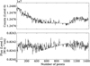 |
Fig. A.1. Top: Measured counts (level 0 data), before any corrections. Bottom: Counts transformed into flux (level 1 data), after correction for external effects. |
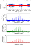 |
Fig. A.2. Top: Measured intensity in the three VIRGO/SPMs channels (blue, green and red). Bottom three panels: PSD computed from each channel and the x-axis is limited to the p-mode frequency range. |
Furthermore, there are also missing values in the data corresponding to the SoHO recovery mission when there were no measurements for about 100 days in 1998, and the upload of a new software in January 1999. The asteroseismic proxy used in this work (and described in Sect. 2) is inferred from the mean of red and green channels of VIRGO/SPMS, so that missing values are ignored: for the times when one of both channels has a gap, the value of the other channel is kept. Some gaps are common in both channels, and there are still 2.25 % of missing values in this final time series. After cutting the VIRGO/SPMs asteroseismic proxy into 28 equally long subseries of approximately 376.56 days, we interpolated all missing values due to the attractors (gaps smaller than 6 days), by applying a multi-scale discrete cosine transform following inpainting techniques (Elad et al. 2005), which is commonly used for data reduction in asteroseismology (e.g. García et al. 2014). As recommended by Pires et al. (2015), we performed 100 iterations, for each subseries, in the inpainting procedure. 43.4 % of the missing values are filled by this method. Remaining gaps (larger than 6 days) due to the SoHO recovery mission and the update of the new software were replaced by zeros.
A.2. Photon noise
The contribution of photon noise constitutes the dominant component of the signal at frequencies above approximately 8000 μHz (García & Ballot 2019), allowing for the estimation of the photon noise level in the time series. The VIRGO/SPMs data acquisition system (DAS) operates with a cadence of 3 minutes, corresponding to a fundamental frequency of 5555.55 μHz. The associated Nyquist frequency, defined as half the sampling rate, is 2777.78 μHz. Given the periodic nature of the data sampling, the system introduces harmonics of the fundamental cadence frequency at 5555.55 μHz and an additional harmonic at 8333.33 μHz, which corresponds to a frequency near the Nyquist limit of VIRGO/SPMs. To avoid contamination from these harmonics, particularly the aliasing effect at 8333.33 μHz, the estimation of photon noise is restricted to frequencies below 8200 μHz. This cut-off ensures that the influence of harmonics and aliasing is minimised, thereby providing an accurate representation of the photon noise contribution (Salabert et al. 2017).
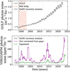 |
Fig. A.3. Photon noise estimation from the mean PSD in 8000-8200 μHz range over successive sub-series of 125 days with 15.625 days overlap. The top panel displays the photon noise of the GOLF instrument and the bottom panel, the ones from the mean corrected and not-corrected time series of green and red channels of VIRGO/SPMs. The grey zones in each panel indicate the period when SoHO was shut down due to the satellite recovery mission, and the red hatched area in the top panel highlights the dates of the red wing measurements from GOLF. |
For these reasons, to assess the variation in photon noise over the lifetime of the two instruments, estimates were calculated as the mean value of the Power Spectral Density (PSD) in the 8000-8200 μHz range, from 125-day sub-series overlapping by 1/8 the length of the sub-series. The variation in photon noise for GOLF is shown in the upper panel of Fig. A.3, and the one from the VIRGO/SPMs asteroseismic proxy is in the lower panel. From this, we see an increase in photon noise of GOLF measurements over time, and a one-year modulation. From the first year of data, to the last one, the mean photon noise per year increased by about 8.6. For VIRGO/SPMs measurements, two different photon noises are shown: the first (green), computed from the time series without correction (σph, nc), where missing values were replaced by zeros; and the second (violet), calculated from the inpainted time series (σph, in). The corresponding mean photon noise is divided by about 2.8 between the two data reductions:

The cyclic variation in photon noise from VIRGO/SPMs appears to be linked to the solar magnetic cycle in both cases, with a more significant impact observed during the maximum of cycle 25. Given that the method used to address gaps in the data heavily affects the photon noise and, consequently, our analysis, we rely solely on the interpolated VIRGO/SPMs dataset for our analysis.
Appendix B: The solar radio-flux as a proxy for magnetic cycle
In this section, we describe how the low- and high- magnetic activity epoch were defined based on the solar radio flux index measurements.
The solar radio-flux index (F10.7, Tapping 2013) represents the total solar radio emission, integrated over one hour, at a wavelength of 10.7 cm and averaged at a distance of 1 AU. Since directly observed measurements of F10.7 radio emissions are influenced by variations in the Sun-Earth distance, we opted to use the adjusted flux provided by Natural Resources Canada (NRCan), which accounts for the average distance. Complete measurements are publicly available in the NRCan FTP server3, in solar flux unit (sfu) where 1 sfu = 10−22 W m−2 Hz−1. Data are separated into several files because the latest observations (later than October 28th, 2004) are also directly available from NRCan website4. We concatenated two tables to cover the entire SoHO observation period: one containing data from 1996 to 2007, and the second containing latest data from 2004 to today, dropping common values. We then calculated the average  index, which represents the mean of the solar radio flux index over a 100-day window, shifted for each day. The length of the smoothing window was selected to be sufficiently large, closely matching the 108-day window chosen by (Kiefer & Broomhall 2021) for similar smoothing. F10.7 and
  are shown in Fig. B.1, depicted in light and dark brown, respectively.
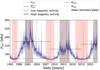 |
Fig. B.1. Proxy for the solar magnetic activity: the solar radio-flux given by the F10.7 index (Tapping 2013) is shown in transparent blue. The dark blue curve shows the mean solar radio-flux filtered with a 101-days window |

Thresholds used to define starting and ending dates of each cycle extremum for cycles 23, 24, and 25.
We defined epochs of magnetic activity extrema from the solar radio flux index, for clarity in the comparisons (see Sects. 4.3 and 4.4). For this, we chose threshold values for the  that define the high (and low) periods of magnetic activity. For low activity, the threshold Θmin is chosen as the 20 % quantile of the
  values, taken from the starting observation date of VIRGO/SPMs: Θmin = 74.92 sfu. Low-activity dates correspond to the extreme dates for each cycle when
  falls below the threshold. Figure B.1 highlights these low magnetic activity periods, Θmin, and Table B.1 reports thresholds values and epochs duration. Figure B.1 illustrates that the durations of low-activity epochs are not all the same: approximately three years for the minimum of cycle 24 versus four years for the minimum of cycle 24. Since epochs of high magnetic activity do not always have the same amplitude, we first define the cycle epochs as the time between two minima, namely, the time between the successive means of the previously defined low-activity dates. For instance, the epoch of cycle 23 spans from the average extremum dates of the minimum of cycle 23 and the average extremum dates of the minimum of cycle 24, namely, from 1996-07-18 to 2008-07-16. The dashed grey lines in Fig. B.1 separate cycle periods and since we are currently in cycle 25, the last date of the epoch stops on July 16th, 2024. We then define the thresholds for the high magnetic activity dates as the quantile values at 85 % for each cycle period. Thresholds are drawn on Fig. B.1 as well as the periods of high magnetic activity.
Appendix C: Depth of maximum mode sensitivity
Acoustic modes are sensitive to different regions of the star, in particular higher-frequency modes are more sensitive to the outer layers of the star. Variations in the magnetic field in some regions should then have a greater influence on the behaviour of modes that are sensitive to the same regions (Christensen-Dalsgaard 2008). Basu et al. (2012) first computed the sound-speed kernels for several modes grouped by frequency bands, thus determining the sensitivity of these mode groups across the solar radius. When studying the modes n = 11 to n = 26, grouped into three frequency bands: 1800-2450 μHz, 2450-3110 μHz, and 3110-3790 μHz, García et al. (2024) showed that their maximum sensitivity occurs in a region located 74 km to 1575 km beneath the surface (using the model of Bahcall & Serenelli 2005). In our study, only modes n = 14 to n = 25 were considered. To identify the relative location of the non-stochastic excitation of the modes, their energy time series were grouped in sets of 12 and combined into three frequency bands: 2090-2620 μHz, 2620-3160 μHz, and 3160-3710 μHz.
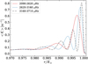 |
Fig. C.1. Mean sound-speed kernels < 𝒦> for three frequency bands: 2090-2620 μHz as red continuous line, 2620-3160 μHz as blue dashed line, and 3160-3710 μHz as black long dashed line. For each frequencies band, only ℓ = 0, 1 and 2 were considered. |
The mean sound-speed kernels < 𝒦> per frequency range are shown in Fig. C.1. We briefly remind here the analytic expression of the sound-speed kernels of oscillation modes, as derived by e.g. Gough & Thompson (1991). 𝒮 is defined as:
![Mathematical equation: $$ \begin{aligned} \mathcal{S} = \int \left[\xi _r^2 + \ell (\ell +1)\, \xi _h^2 \right] \rho r^2 dr\,, \end{aligned} $$](/articles/aa/full_html/2025/08/aa55189-25/aa55189-25-eq27.gif) (C.1)
(C.1)
where ξr and ξh are the radial and horizontal components of the displacement δr induced by a small perturbation of the equilibrium state. The sound-speed kernel Kc2, ρ(r) is thus expressed for each mode (n, ℓ) as:
 (C.2)
(C.2)
where ω is the angular frequency, ρ the density and r the radius. The adiabatic sound speed c is described as:
 (C.3)
(C.3)
where Γ1 = (∂lnp/∂lnρ)ad and P is the pressure. According to Christensen-Dalsgaard (2008), χ(r) is the magnitude of div(δr) defined by:
 (C.4)
(C.4)
The oscillation parameters were computed with GYRE (Townsend & Teitler 2013) from the S-model5 (Christensen-Dalsgaard et al. 1996). The maximum sensitivity for our lower to higher frequency bands are 1895 km, 1014 km, and 605 km beneath the surface, respectively. These results are closer to those found by Basu et al. (2012) than those by García et al. (2024), as they are highly dependent on the chosen solar structure model.
Appendix D: High-energy peaks detected in the combined time series of VIRGO/SPMs
The high energy peaks from 𝒮phot that are detailed in Section 5, are listed in Table D.1.
List of the dates of the detected high energy peaks in 𝒮phot, and correspondence of the detected peaks in other indicators discussed in the text.
Appendix E: Timescale condition for the excitation source
Given that the modes are characterised by a timescale of approximately T0 = 5 minutes, we aim to infer a constraint on the timescale of the excitation source required to effectively excite these modes. We assume an oscillation driven by the equation of a forced harmonic oscillator given by:
 (E.1)
(E.1)
where ω0 = 2π/T0 is the natural frequency of the oscillator and f(t) is the forcing function. A solution of this is:
 (E.2)
(E.2)
Assuming that the forcing function describing the excitation source takes the form:
 (E.3)
(E.3)
where Δτ = 2π/ω, Y0 is a constant, and ae(t) is the acceleration of the excitation source. The corresponding characteristic speed ve(t) is thus:
![Mathematical equation: $$ \begin{aligned} v_\mathrm{e} (t) \equiv \int _0^t a_\mathrm{e} (t) \mathrm{d} t = Y_0\,\omega [1-\cos (\omega t)]\,, \end{aligned} $$](/articles/aa/full_html/2025/08/aa55189-25/aa55189-25-eq34.gif) (E.4)
(E.4)
and its characteristic amplitude Ye(t) is:
![Mathematical equation: $$ \begin{aligned} Y_\mathrm{e} (t) \equiv \int _0^t v_\mathrm{e} \,\mathrm{d} t = Y_0[\omega t- \sin (\omega t)]\,, \end{aligned} $$](/articles/aa/full_html/2025/08/aa55189-25/aa55189-25-eq35.gif) (E.5)
(E.5)
where Yemax = Ye(t = Δτ) = 2πY0 is the maximum amplitude of the excitation source.
All constant terms apart, the first integral of Eq. (E.2) gives:
![Mathematical equation: $$ \begin{aligned}&\int _0^{\Delta \tau } \sin (\omega t^{\prime })\,e^{-i\omega _0 t^{\prime }} \mathrm{d} t^{\prime } = \int _0^{\Delta \tau } \left(\frac{e^{i\omega t^{\prime }}-e^{-i\omega t^{\prime }}}{2i}\right)\,e^{-i\omega _0 t^{\prime }} \mathrm{d} t^{\prime } \nonumber \\&\quad = \frac{\omega -e^{-i\omega _0 \Delta \tau } [\omega \cos (\omega \Delta \tau ) + i\omega _0 \sin (\omega \Delta \tau ) ]}{(\omega ^2-\omega _0^2)} \,. \end{aligned} $$](/articles/aa/full_html/2025/08/aa55189-25/aa55189-25-eq36.gif) (E.6)
(E.6)
As ωΔτ = 2π, this leads to:
 (E.7)
(E.7)
In the same way, the second integral of Eq. (E.2) reduces to:
 (E.8)
(E.8)
Thus, when t > Δτ, Eq. (E.2), gives:
![Mathematical equation: $$ \begin{aligned} \begin{aligned} y(t)&= \frac{Y_0\,\omega ^3}{2i\omega _0(\omega ^2-\omega _0^2)} \left\{ e^{i\omega _0 t} \left(1 -e^{-i\omega _0 \Delta \tau }\right) - e^{-i\omega _0 t} \left(1 -e^{i\omega _0 \Delta \tau }\right) \right\} \\&= \frac{Y_0\,\omega ^3}{2i\omega _0(\omega ^2-\omega _0^2)} \bigg \{ 2i\sin (\omega _0t) - 2i \sin [\omega _0(t-\Delta \tau )]\bigg \}\,. \end{aligned} \end{aligned} $$](/articles/aa/full_html/2025/08/aa55189-25/aa55189-25-eq39.gif) (E.9)
(E.9)
Let x ≡ ω0/ω = Δτ/T0:
![Mathematical equation: $$ \begin{aligned} \begin{aligned} y(t)&= \frac{Y_0}{x(1-x^2)} \bigg \{\sin (\omega _0t) - \sin \left(\omega _0 t- 2\pi x\right)\bigg \} \\&= \frac{Y_0}{x(1-x^2)} \bigg \{2\cos (\omega _0t-\pi x) \sin (\pi x)\bigg \} \\&= \frac{2\pi Y_0}{1-x^2}\, \bigg [\frac{\sin (\pi x)}{\pi x}\bigg ] \,\cos (\omega _0t-\pi x)\,. \end{aligned} \end{aligned} $$](/articles/aa/full_html/2025/08/aa55189-25/aa55189-25-eq40.gif) (E.10)
(E.10)
Considering η(x):
![Mathematical equation: $$ \begin{aligned} \eta (x) \equiv \frac{1}{1-x^2}\bigg [\frac{\sin (\pi x)}{\pi x}\bigg ]\,, \end{aligned} $$](/articles/aa/full_html/2025/08/aa55189-25/aa55189-25-eq41.gif) (E.11)
(E.11)
one can write:
 (E.12)
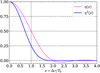 |
Fig. E.1. Function η (pink line) describes the amplitude of the oscillator relative to the amplitude of the source term for t > Δτ. The blue curve describing η2 is a measure of the efficiency of the impulsive excitation. |
The function η shown in Fig. E.1 describes the fraction of the amplitude of the forcing term that is transferred to the mode amplitude. The quantity η2, also shown in Fig. E.1 can thus be viewed as an efficiency of the energy transfer from the source term to the modes. This efficiency is maximum for Δτ ≪ T0. It decreases by approximately 30 % when Δτ = T0/2, drops to about 25 % when Δτ = T0 and rapidly approaches zero for larger values of the Δτ/T0 ratio. This calculation illustrates the fact that the impulsive excitation of an oscillator is inefficient if the timescale of the impulsion is larger than the oscillation period.
All Tables
Starting and ending dates of the gaps greater than one day in the VIRGO/SPMs data.
Thresholds and used to define starting and ending dates of each cycle extremum for cycles 23, 24, and 25.
List of α and β parameters along with resulting p-values of the performed KS tests.
Resulting p-values of the KS tests performed to compare combined energy time series in the three frequency bands 2090–2620 μHz, 2620–3160 μHz, and 3160–3710 μHz, with the best distributions.
Thresholds used to define starting and ending dates of each cycle extremum for cycles 23, 24, and 25.
List of the dates of the detected high energy peaks in 𝒮phot, and correspondence of the detected peaks in other indicators discussed in the text.
All Figures
|
Fig. 1. PSD of the VIRGO/SPMs light curve (from 23.01.1996 to 23.11.2023). Higher frequencies are displayed between 3270 and 3750 μHz, showing the large frequency separation (δν) noted between modes ℓ = 0 and ℓ = 1 for n = 23. Modes are marked by vertical lines with different colours: n = 22 in light blue, n = 23 in orange, n = 24 in yellow, n = 25 in cyan, and n = 26 in dark blue). ℓ = 0 are in continuous, ℓ = 1 in dashed, ℓ = 2 in dotted, and ℓ = 3 in dot-dashed lines. In the subplot: Window of Δω = 8 μHz used to reconstruct modes energy time series is shown around modes (n = 25, ℓ = 0) in light brown and (n = 24, ℓ = 2) in dark brown. |
| In the text | |
|
Fig. 2. Top panel: Simulated sinusoidal signal S(t) with a period of 0.5 days and three excitations randomly distributed in time. It is shown for a time series of 10 days sampled at 60 seconds. The excitations are exponentially decaying. Bottom panel: Energy E(t) = 2|S(t)|2 corresponding to the simulated signal is shown in grey and the reconstructed energy is shown in dashed black. |
| In the text | |
|
Fig. 3. Normalised reconstructed energy time series for n = 22, ℓ = 0, with VIRGO/SPMs data. For better visibility, we restricted the x-axis between 2007 and 2015. The series were reconstructed from 23 January1996 to 17 February 2016. |
| In the text | |
|
Fig. 4. Resulting p-values of the Kolmogorov-Smirnov tests comparing reconstructed time series distributions with exponential distributions. Orange triangles stand for ℓ = 0 modes, dark blue squares for ℓ = 1 modes, and light blue circles for ℓ = 2 modes. The threshold of rejection of 5% is drawn as a dashed black line. |
| In the text | |
|
Fig. 5. Resulting p-values of the Kolmogorov-Smirnov tests comparing reconstructed time series distributions with exponential distributions, for measurements taken during low and high magnetic activity periods whose dates are listed in Table 2. Triangles stand for ℓ = 0 modes, squares for ℓ = 1 modes, and circles for ℓ = 2 modes. Brown and pink makers stand for tests on values taken during high (resp. low) magnetic activity. The threshold of rejection of 5% is drawn as a dashed black line. |
| In the text | |
|
Fig. 6. Q-Q plot comparing the combined energy time series with |
| In the text | |
|
Fig. 7. Distributions of normalised combined energies. For each cycle period, we show the histogram, the best |
| In the text | |
|
Fig. 8. Mean (top panel) and variance (bottom panel) of a one-year subseries slided every eighth of a year of the energy supply rate computed from the combined time series of the modes. These quantities are plotted against the central date of the considered subseries and the x-axis error bars show the range of dates taken for each subseries. Periods of low (pink) and high (brown) magnetic activity are reported from Table 2 and |
| In the text | |
|
Fig. 9. Spearman’s rank correlation ρ between 𝒮phot and 𝒮vel data, versus radial order n for all considered modes. Blue circles stands for ℓ = 0 modes, red triangles for ℓ = 1, and green stars for ℓ = 2. Markers in the grey area correspond to a p-value larger than 10−3%. |
| In the text | |
|
Fig. 10. Distribution of the detected peaks over time for the three frequency bands, from top to bottom: 2090–2620 μHz, 2620–3160 μHz, and 3160–3710 μHz. Each bin corresponds to one year from 1995 to 2025. Dashed curve shows the Epanechnikov kernel density estimations (KDE) of the probability distributions from each histogram. Periods of low and high magnetic activity were reported from Table 2 and |
| In the text | |
|
Fig. 11. 𝒮phot is shown in light blue in the lower part of each panel, along with the detected high-energy peaks marked by dark blue crosses. For better clarity, the full 27-year time series is divided into three panels (from top to bottom). For each peak, when it corresponds to a peak in σphot (resp. in 𝒞phot or in 𝒮vel), within a window of δt = 1.45 days, a red (resp. pink or brown) circle highlights it in the top light beige area of each panel. Similarly, when at least one X-class flare (or one CME) occurred within the δt-window around the peak, it is marked by an orange (or green) circle. Peaks not coinciding with any of these events are marked by violet circles. Furthermore, if a peak is detected within one of the three defined frequency bands, it is highlighted with a black marker: a square for low frequencies, a star for medium frequencies, and a triangle for high frequencies. Gaps due to the SoHO recovery mission are represented as grey shaded areas. Minor ticks represent months. |
| In the text | |
|
Fig. A.1. Top: Measured counts (level 0 data), before any corrections. Bottom: Counts transformed into flux (level 1 data), after correction for external effects. |
| In the text | |
|
Fig. A.2. Top: Measured intensity in the three VIRGO/SPMs channels (blue, green and red). Bottom three panels: PSD computed from each channel and the x-axis is limited to the p-mode frequency range. |
| In the text | |
|
Fig. A.3. Photon noise estimation from the mean PSD in 8000-8200 μHz range over successive sub-series of 125 days with 15.625 days overlap. The top panel displays the photon noise of the GOLF instrument and the bottom panel, the ones from the mean corrected and not-corrected time series of green and red channels of VIRGO/SPMs. The grey zones in each panel indicate the period when SoHO was shut down due to the satellite recovery mission, and the red hatched area in the top panel highlights the dates of the red wing measurements from GOLF. |
| In the text | |
|
Fig. B.1. Proxy for the solar magnetic activity: the solar radio-flux given by the F10.7 index (Tapping 2013) is shown in transparent blue. The dark blue curve shows the mean solar radio-flux filtered with a 101-days window |
| In the text | |
|
Fig. C.1. Mean sound-speed kernels < 𝒦> for three frequency bands: 2090-2620 μHz as red continuous line, 2620-3160 μHz as blue dashed line, and 3160-3710 μHz as black long dashed line. For each frequencies band, only ℓ = 0, 1 and 2 were considered. |
| In the text | |
|
Fig. E.1. Function η (pink line) describes the amplitude of the oscillator relative to the amplitude of the source term for t > Δτ. The blue curve describing η2 is a measure of the efficiency of the impulsive excitation. |
| In the text | |
Current usage metrics show cumulative count of Article Views (full-text article views including HTML views, PDF and ePub downloads, according to the available data) and Abstracts Views on Vision4Press platform.
Data correspond to usage on the plateform after 2015. The current usage metrics is available 48-96 hours after online publication and is updated daily on week days.
Initial download of the metrics may take a while.