| Issue |
A&A
Volume 701, September 2025
|
|
|---|---|---|
| Article Number | A63 | |
| Number of page(s) | 23 | |
| Section | Astronomical instrumentation | |
| DOI | https://doi.org/10.1051/0004-6361/202553987 | |
| Published online | 03 September 2025 | |
Calibration and performances of the integrated Mach—Zehnder wavefront sensor for extreme adaptive optics
Centre de recherche astrophysique de Lyon (CRAL), Université Claude Bernard Lyon 1, CNRS, ENS,
9 avenue Charles Andre,
69561
Saint Genis Laval,
France
★ Corresponding author: This email address is being protected from spambots. You need JavaScript enabled to view it.
Received:
31
January
2025
Accepted:
20
June
2025
Abstract
Context. Direct imaging of circumstellar environments around nearby stars requires eXtreme Adaptive Optics (XAO) systems. These systems must integrate advanced wavefront sensors (WFSs) to reach a high Strehl ratio (SR) in the near-infrared and at visible wavelengths on future giant segmented mirror telescopes (GSMTs). Direct detection of faint exoplanets with these extremely large telescopes will require tens of thousands of correction modes. In addition, highly accurate and sensitive WFSs set key requirements. The precise measurement of the wavefront degradation for both static and dynamic aberrations with a limited number of photons is still an issue for most WFSs, which are often limited either in sensitivity or in dynamical range.
Aims. We present the integrated Mach–Zehnder (iMZ), a self-referenced interferometric WFS developed for XAO and implemented on an XAO test bench at CRAL. The WFS concept consists of creating two opposite sets of interferences between the wavefront phase to be measured and the spatially filtered reference beam. We describe the implementation of this concept, including the scheme we have developed to extend its dynamical range by using phase diversity.
Methods. We present an iMZ physical model that allows the performance of this sensor to be studied in closed loop for different telescopes (the Very Large Telescope (VLT) and the Extremely Large Telescope (ELT)) in different turbulence regimes and including island effects, cophasing residuals, or low wind effects. A calibration method adapted to the iMZ that takes into account the nonlinearities of the signal was developed to use this WFS for diverse types of phase measurements. We analytically computed the photon noise error propagation of the iMZ, setting its ultimate sensitivity, and we compared it with several WFSs used in adaptive optics. Finally, we demonstrated the performances of the iMZ in closed loop by using end-to-end (E2E) simulations and experimental validations.
Results. The proposed iMZ WFS demonstrates a significant gain in sensitivity compared to the Shack–Hartmann WFS traditionally used in AO. The iMZ dynamical range, reduced to a wavelength in closed-loop operations, can be extended to several wavelengths by using phase diversity strategies developed in this paper. We demonstrate, with simulations and experimentally, a new calibration method for the iMZ, which is an essential step for the precise reconstruction of the phase. It is achieved by solving an inverse problem based on the interferometric model of the data. Our E2E numerical simulations confirm the very good performances of this sensor and the possibility of using it without a first stage of correction in good turbulence conditions. Experimental laboratory results demonstrate the efficiency of the iMZ in closed loop under good seeing conditions. The development of the iMZ is also motivated by the arrival of GSMTs leading to challenging new optical aberrations, such as differential pistons between different segments constituting the pupil and the pupil fragmentation (also called petal modes). The iMZ can efficiently measure these type of aberrations as well, to which most WFSs are not sensitive or are only slightly sensitive because their responses are generally proportional to the derivative of the incident wavefront. With its two complementary outputs, the iMZ WFS also offers the possibility of measuring the amplitude of the incident wave jointly with its phase without sensitivity loss, which makes it possible to consider correcting the effects of scintillation due to the atmosphere.
Conclusions. We conclude that the iMZ is an excellent WFS candidate for future XAO systems, in particular on GSMTs.
Key words: instrumentation: adaptive optics / methods: analytical / methods: data analysis / methods: numerical / techniques: high angular resolution / techniques: interferometric
© The Authors 2025
 Open Access article, published by EDP Sciences, under the terms of the Creative Commons Attribution License (https://creativecommons.org/licenses/by/4.0), which permits unrestricted use, distribution, and reproduction in any medium, provided the original work is properly cited.
This article is published in open access under the Subscribe to Open model. This email address is being protected from spambots. You need JavaScript enabled to view it. to support open access publication.
1 Introduction
Extreme adaptive optics (XAO) is used for exoplanet direct detection to achieve high-contrast imaging (HCI) by correcting the degradation of astronomical images caused by atmospheric turbulence, in order to restore almost perfectly the diffraction limit of ground-based telescopes, and thus maximize their angular resolving power and their high-contrast capability. Over the past two decades, several HCI instruments have been developed for 8 m class telescopes, such as the spectro-polarimetric research on high-contrast exoplanets (SPHERE; Beuzit et al. 2019), the GEMINI Planet Imager (GPI; Macintosh et al. 2018), the SUBARU Coronagraphic Extreme Adaptive Optics (SCExAO; Jovanovic et al. 2015), the Keck Planet Imager and Characterizer (KPIC; Mawet et al. 2018), or the Magellan extreme adaptive optics (AO) system (MagAO-X; Males et al. 2018), which have led to the discovery of several young giant planets (e.g., Lagrange et al. 2010; Macintosh et al. 2015; Keppler et al. 2018). The future generation of giant telescopes (30-40 m class), with the Extremely Large Telescope (ELT), the Giant Magellan Telescope (GMT), and the Thirty Meter Telescope (TMT), will see first light in the 2030s and should be able to detect and characterize smaller planets with sizes as small as the Earth around the nearest M dwarfs, located in the habitable zone (Kasper et al. 2021). To achieve a high contrast up to very small separations (a few tens of milli-arcseconds), HCI combines XAO (Guyon 2005) with coro-nagraphy (Mawet et al. 2012) and post-processing (Marois et al. 2006; Flasseur et al. 2020; Dallant et al. 2023). These techniques significantly increase the detection sensitivity, provided that the XAO system delivers a very high Strehl ratio (SR) at the focal plane of the instruments. For example, the AO system of SPHERE, SAXO (Fusco et al. 2014), achieves regularly 90% of Strehl in the H band for bright stars. The goal of the ELT planetary camera spectrograph (PCS; Kasper et al. 2021) is similar to SPHERE but at shorter wavelengths, to enable the detection of exo-Earths and bio-markers in the atmosphere of exoplanets.
One major limitation of today’s XAO systems lies in their ability to precisely measure the deformation of the incoming wavefront, which is strongly conditioned by the telescope diameter and nature (monolithic or segmented primary mirror). The wavefront sensors (WFSs) used to measure the deformations degrading the image contrast must be sensitive to phase variations ranging from several tens of micrometers to a few nanometers, with a very low number of photons collected in a limited amount of time to measure and correct the turbulence before its evolution. The Shack–Hartmann wavefront sensor (SHWFS), traditionally used for the first AO systems, is the most robust and linear of the WFSs used in AO. However, this sensor is limited in terms of sensitivity and noise propagation. Today, the most popular sensor is the pyramid wavefront sensor (PyWFS; Ragazzoni 1996), which will equip most AO systems of the next generation of high-contrast instruments for the extremely large telescopes. The unmodulated pyramid sensor presents a greater sensitivity than the Shack–Hartmann but is limited in dynamic range. On the other hand, it can be modulated to increase its linear range at the expense of a decrease in sensitivity, as is presented in Plantet et al. (2015). In the context of giant segmented mirror telescopes, the Zernike wavefront sensor (ZWFS) also represent a promising option. A concept called the Zernike unit for segment phasing (ZEUS) was previously developed for ground-based applications to operate under seeing-limited images (Dohlen et al. 2006; Vigan et al. 2010). This concept was revisited by Janin-Potiron et al. (2017) to measure segment-wise the piston, tip, and tilt in the diffraction-limited regime, allowing for the correction of these aberrations in closed-loop operations.
The integrated Mach–Zehnder (iMZ) is a WFS developed for XAO, enabling high-precision phase measurement at the nanometer scale (Fang et al. 2019). This sensor, first proposed in astronomy by Angel (1994) and inspired by the Zernike test (Zernike 1934), is based on the Mach–Zehnder interferometer (Mach 1892; Zehnder 1891), in which one of the two arms is spatially filtered with a pinhole, to create a reference wavefront. This additional spatial filter leads to the self-reference Mach– Zehnder WFS. The pinhole diameter can be adjusted depending on the wavefront distortion to be measured. Traditionally set to λ/D for atmospheric turbulence measurement, with λ the wavelength and D the pupil diameter, larger pinhole diameters can be used to measure high-frequency aberrations such as for co-phasing segments (e.g., Dohlen et al. 1998). In this article, we study a solid glass Mach–Zehnder prototype called integrated (iMZ) derived from Angel (1994), and implemented on the CRAL XAO test bench (Langlois et al. 2023). This pupil plane WFS has two complementary outputs, encoding the pointwise sine of the wavefront phase. The iMZ presents a certain number of advantages, such as a good sensitivity due to its interferometric nature, a linear response for small phase distortions (e.g., in the AO closed-loop regime), and the possibility of measuring the amplitude of the incident wavefront together with its phase, which can then be used to correct for atmospheric scintillation effects. Its major limitation comes from its dynamic range, reduced to one wavelength in closed-loop operation. This issue is discussed in this article, and strategies to extend this dynamical range, such as phase diversity and phase unwrapping, are presented. The development of the iMZ WFS is also motivated by the segmented 30-meter class telescopes coming out in the next few years, which will produce various aberrations, such as differential piston errors between the different fragments and segments of the pupil of these telescopes (also known as petal modes, Schwartz et al. (2018) or local aberrations linked to low wind effects (Sauvage et al. 2015; Milli et al. 2018). For such configurations, the absolute wavefront measurements at each position of the pupil enable the iMZ to measure precisely these type of aberrations, to which the classical wavefront sensors mentioned earlier are not sensitive, their responses being in general proportional to the spatial derivative of the incident wavefront.
In Sect. 2, the iMZ WFS is presented in detail, and the model equations are established. The phase measurement range (dynamical range) of the iMZ is discussed, and strategies to overcome the sine limited range are presented and illustrated with experimental results. In Sect. 3, we study noise propagation in the iMZ signal to estimate its sensitivity. The iMZ is then compared with other AO WFSs (Shack–Hartmann, nonmodulated pyramid, Zernike mask, etc.) in terms of sensitivity. The impact of spectral bandwidth broadening on the iMZ signal is then discussed in Sect. 4, through preliminary simulated results. Sect. 5 focuses on the calibration method developed for the iMZ. The proposed calibration method is based on an inverse problem approach and provides the least mean squares estimators of the model parameters. The calibration is tested on simulated and experimental data. Closed-loop simulation results with the iMZ on an 8-meter pupil telescope without first stage correction for different turbulence and flux corrections are presented in Sect. 6, demonstrating the good performance of the iMZ in good seeing conditions. Experimental results of closed-loop phase correction obtained on the XAO test bench at CRAL are then introduced. Finally, the iMZ response to differential piston modes (also known as petal modes) is presented in Sect. 7.3, with experimental results obtained on the XAO bench.
2 The integrated Mach–Zehnder (iMZ) wavefront sensor
In this section, we describe the iMZ device and derive its mathematical model.
2.1 The iMZ device
An iMZ is a solid-state version of the classic Mach–Zehnder interferometer (Mach 1892; Zehnder 1891) with one arm filtered by a pinhole to create a phase reference. This solid configuration brings the stability required to produce interference fringes in white light (with few microns of coherence length) and also eliminates the issue of differential aberrations between the two interferometric arms, due to local turbulence on the free space version of the Mach–Zehnder.
Our iMZ device, shown in Fig. 1, is made of two glass plates assembled together by molecular adhesion, with a single SiO2 λ/4 beam splitter layer coated in between. Approximately 30% of the incident beam is reflected on the beam splitter layer, while the rest of it is transmitted toward side 1 to create the reference phase. On this side of the component, a small silver reflective dot acting as a pinhole is obtained by an aluminum coating deposit (see Fig. 1c). This pinhole acts like a spatial filter for the incoming beam to create a reference wavefront by reflection. The filtering of the amplitude by this pinhole conditions the sensitivity of the WFS, by setting the number of spatial modes seen by the iMZ (filtered out in the reference) and the amount of photons available from the point spread function (PSF) core for the phase measurement. The part of the light not reflected by the pinhole can be re-imaged behind Side 1 for flux normalization and/or tip-tilt control, as done on our bench. This additional output, to which we refer as the coronagraphic output as it may also be used for coronagraphy, is made up of the photons from outside of the mask and the photons that have passed through the mask (3–5% of transmission). These photons are not used to measure the phase aberrations. The opposite iMZ side is fully coated with a Ti3O5 λ/8 phase shifting layer and a silver reflective layer. The Ti3O5 layer provides a π/2 phase shift necessary to create, after recombination, two complementary interferograms encoding the phase sine (and not the cosine). A signal varying with the sine of the phase is much more effective than a cosine signal to measure small phase variations around zero, corresponding to the AO closed-loop regime. Indeed, the sine function is linear for small variations in the phase, φ, around zero, while the cosine function is approximately 1 - φ2/2 which is ambiguous and nearly insensitive to small variations in φ. For example, for a variation of one tenth of a radian, the intensity variation in a sine signal is 20 times greater than that of a cosine signal.
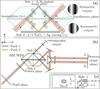 |
Fig. 1 Schematic representation of the iMZ WFS. (a) The iMZ component. (b) Light path from the pupil plane preceding the iMZ to the detector. (c) Lateral view of the pinhole side of the iMZ, with ρ1 the amplitude reflection coefficient on Side 1 (see later Table 1). |
2.2 The iMZ model
We now derive a formal model of the iMZ outputs. Table 1 summarizes the notations and Fig. 1a shows the different paths followed by the wave.
To account for the complex transmittances and reflectances of the different optical parts of the iMZ, we first considered the complex amplitude of a simple ray toward the center of the pinhole. To simplify the developments, we omitted the phase shifts due to the propagation along the paths (the two sides of the iMZ being identical in that respect). The transmitted and reflected complex amplitudes of the ray after the first interaction with the beam splitter are
 (1)
(1)
where u is the complex amplitude of the inward ray, while t and r are the respective complex transmittance and complex reflectance of the beam splitter. After reflection on the external coatings on both sides of the device, the complex amplitudes become
 (2)
(2)
with r1 and r2 the respective complex reflectances of the coating on Side 1 (pinhole) and on Side 2. Finally, the complex amplitudes of the two emerging rays are
 (3)
(3)
where a symmetric beam splitter has been assumed, that is with the same complex transmittance, t, and complex reflectance, r, for an inward wave from Side 1 than for an inward wave from Side 2.
We now consider the complex field (hence in bold face) of the wave as a function of the position in a transverse plane with respect to the direction of propagation along the different paths. Combining Eqs. (1), (2), and (3), the complex amplitudes of the two images formed on the detector are given by
 (4)
(4)
where u is the complex amplitude of the pupil re-imaged on the detector and u is like u but also accounts for the spatial filtering by the pinhole mask. In the proposed setup, the pinhole is in a focal plane; thus,
 (5)
(5)
with * the two-dimensional convolution and F(p) the twodimensional Fourier transform of the pinhole mask, p, which takes values between zero, where the pinhole is fully transparent, and one, where the pinhole is fully reflective.
Taking the squared modulii of the output complex amplitudes yields the intensities of the images formed on the detector:
![Mathematical equation: \bm{I}_{\Sym} &= \Abs*{\bm{u}_{1}}^{2} = \bm{\alpha}_{\Sym} + \bm{\beta}\,\cos\Paren[\big]{ \bm{\varphi} - \filtered{\bm{\varphi}} + \varphi_{2} - \varphi_{1}},\\](/articles/aa/full_html/2025/09/aa53987-25/aa53987-25-eq6.png) (6a)
(6a)
![Mathematical equation: \bm{I}_{\Asym} &= \Abs*{\bm{u}_{2}}^{2} = \bm{\alpha}_{\Asym} + \bm{\beta}\,\cos\Paren[\big]{ \bm{\varphi} - \filtered{\bm{\varphi}} + \varphi_{2} - \varphi_{1} + 2\,(\varphi_{\text{R}} - \varphi_{\text{T}})},](/articles/aa/full_html/2025/09/aa53987-25/aa53987-25-eq7.png) (6b)
(6b)
where the subscripts “s” and “a” denote the symmetric (Side 1) and the asymmetric (Side 2) outputs of the iMZ and with φ = arg(u) the phase of interest,  the phase after filtering by the pinhole, φT = arg(t), φR = arg(r), φ1 = arg(r1) and φ2 = arg(r2). The expressions of the iMZ intensity parameters αs, αa and β are
 (7a)
(7a)
 (7b)
(7b)
 (7c)
(7c)
where  ,
,  ,
,  ,
,  ,
,  , and ρ2 = |r2|. In the above equations, arithmetical operations (such as multiplication) and mathematical functions (such as the square root and the trigonometrical functions) assumed to be applied element-wise. It is worth noting that Eqs. (6a) and (6b) only assume that the beam splitter is symmetric. It is worth noting that, for a 50/50 beam splitter, τ = ρ, and thus αs = αa.
On Side 1, the pinhole behaves like a mirror for the reflected beam, so the phase shift due to the reflection on the pinhole is φ1 = arg(r1) = π. On Side 2, the coating behaves as a mirror behind a wave plate, so the phase shift due to the reflection on this coating is φ2 = arg(r2) = π + 2 φWP, where φWP is the phase shift induced by traversing the wave plate once. In our setup, the wave plate introduces a λ/8 optical path delay, hence, 2 φWP = π/2 and the image intensity in output channel c ∈ {s, a} of the iMZ becomes
 (8a)
(8a)
![Mathematical equation: \bm{I}_{\Asym} &= \bm{\alpha}_{\Asym} - \bm{\beta}\,\sin\Paren[\big]{\bm{\phi} + 2\,(\varphi_{\text{R}} - \varphi_{\text{T}})},](/articles/aa/full_html/2025/09/aa53987-25/aa53987-25-eq42.png) (8b)
(8b)
with  . This particular choice for the waveplate converts the cosine functions of the phase in Eqs. (6a) and (6b) into sine functions which, as previously stated, is more favorable for measuring small phase perturbations.
Finally, for a lossless symmetric beam splitter, Degiorgio (1980) has shown that the phase difference between the reflected and transmitted beams is φR - φT = π/2. This leads to the following unified expression of the image intensity in output channel c ∈ {s, a} of the iMZ with a lossless symmetric beam splitter:
 (9)
(9)
with βs = —β and βa = +β. The phase, φ, measured by the iMZ corresponds to the difference between the input phase, φ, and the filtered phase,  , which is assumed constant over the pupil for a λ/D pinhole. This hypothesis is no longer true for pinholes with large diameters and for high incident aberrations. As the reference phase evolves with the input phase, it cannot be calibrated and must remain negligible compared to the input phase. The results presented in this paper show that the influence of this term on the phase measurement is negligible for pinholes of diameters smaller or equal 1.5 λ/D. The model in Eq. (9) is the one assumed in the remaining of the paper.
Notations and main results for the iMZ model.
2.3 Extraction of the measured phase
Using the approximation sin ϕ ≈ ϕ for ϕ ≈ 0 in the model given by Eq. (9) shows that the iMZ WFS signal is linear with respect to the phase for small phase errors. This approximation, which may be useful in closed-loop regime, is not applicable to measure the phase over the full dynamic range [-π/2, π/2] of the sensor for which the sine function is bijective. In addition, it is worth jointly considering the two outputs of the iMZ to improve the quality of the estimated phase. The nonlinear model in Eq. (9) expresses the light distribution in the two output channels of the iMZ and can thus be exploited to estimate the phase, ϕ, given a WFS image in, say, a maximum likelihood sense. This requires one to describe the statistics of the data as well.
2.3.1 Statistics of the WFS images
To simplify the equations, we assume that the light distribution, I, considered in the iMZ model in Eq. (9) is normalized to have a mean intensity of 1 per pixel and that the detected images are expressed in number of photons (not in ADU). The dark current can be neglected because, for AO wavefront sensing, the WFS images are acquired at a high frame rate. Under these assumptions, the expectation of the data, dc , in the output channel, c ∈ {s, a}, is simply given by
 (10)
(10)
with Ic = αc + βc sin φ the model of the intensity given in Eq. (9) and N, the mean number of inward photons per detector pixel and per frame. It is worth noting that N is measured in the pupil plane, the losses due to the iMZ are taken into account by the factors multiplying the intensities I and I in Eqs. (7a)–(7c).
Under the same assumptions, the variances of the pixel values are given by
 (11)
(11)
where the first term in the last right-hand side is the variance of the photon noise while σron is the standard deviation of the detector read-out noise.
2.3.2 Maximum likelihood estimation of the phase
Neglecting the crosstalk between pixels, the measures provided by the pixels are mutually independent. The statistics of the data can then be approximated by a multi-variate Gaussian with diagonal covariance but non-uniform variance. Computing ϕ, the maximum-likelihood estimator (MLE) of the phases knowing the variance of the data, amounts to solving independent nonlinear weighted least squares problems. These problems being independent, we consider the phase, φ, measured by a single pixel1 in each output channel and at the same position in the pupil plane. Then, the MLE of φ has a closed-form expression on the dynamic range of the iMZ:
![Mathematical equation: \begin{align} \estim{\phi} &= \argmin{\phi \in {\CCRange*{-\frac{\pi}{2},\frac{\pi}{2}}}} \sum_{c\in\{\Sym,\Asym\}} \frac{\Brack*{d_{c} - N\,\Paren*{\alpha_{c} + \beta_{c}\,\sin\phi}}^{2}}{\sigma_{c}^{2}} \notag\\ &= \sin^{-1}\Paren*{\argmin{\xi \in [-1,1]} \sum_{c\in\{\Sym,\Asym\}} \frac{\Brack*{d_{c} - N\,\Paren*{\alpha_{c} + \beta_{c}\,\xi}}^{2}}{\sigma_{c}^{2}}} \notag\\ &= \sin^{-1}\Paren*{\clamp\Paren*{ \frac{\sum_{c\in\{\Sym,\Asym\}} N\,\beta_{c}\,\Paren{d_{c} - N\,\alpha_{c}}/\sigma_{c}^{2}}% {\sum_{c\in\{\Sym,\Asym\}} N^{2}\,\beta_{c}^{2}/\sigma_{c}^{2}}, -1, 1}}, \label{eq:joint-MLE-phi} \end{align}](/articles/aa/full_html/2025/09/aa53987-25/aa53987-25-eq48.png) (12)
(12)
where the function clamp(x, a, b) clamps its argument, x, in the range [a, b] and is defined by
 (13)
(13)
This result has been obtained by noting that the problem to solve is a weighted linear least squares problem in ξ = sin φ under the constraint that ξ ∈ [−1, +1]. The solution of such a constrained problem is simply given by the solution of the unconstrained problem – the fraction in the right-hand side of Eq. (12) - clamped in the range [−1, +1]. This clamping is necessary because, due to the noise, it is possible that the unconstrained solution in ξ be outside the domain of the arcsine function. This is less likely to occur when the measured phase φ is small, for instance in closed-loop operations.
The MLE of the phase estimated from a single output channel c of the iMZ is trivially obtained by restricting the sums in Eq. (12) to this given output. After simplifications this yields
 (14)
(14)
We remark that the MLEs of the phase in Eqs. (12) and (14) assume that the parameters, αc and βc , have been calibrated. A calibration method is proposed in Sect. 5.
2.4 High-dynamical-range phase reconstruction
As is observed in Sect. 2.3, the open-loop dynamical range of the iMZ is theoretically set by the interval [-π/2,π/2] over which the sine is bijective. In practice, the data noise reduces the interval for which the arcsine in Eqs. (12) and (14) yields a correct estimation and thus the dynamic range. Indeed, the more noise in the measurement, the more clamping errors are made in Eq. (12), before applying the arcsine function. These clamping errors translate directly into phase estimation errors. Moreover, the closer is the phase of the sine function to ±π/2 the less sensitive is the WFS.
In closed-loop operations, the working range is extended by a factor of nearly 2 because the sign of the sine is the same as that of the phase on the range (-π, + π) so, inverting the model to retrieve a phase in the range (-π/2, +π/2) may underestimate the phase magnitude but still preserves its sign. The resulting wavefront correction is wrong but still reduces the phase error toward the interval (-π/2, +π/2). Hence, after a few iterations of the AO loop, sufficiently good AO correction should be obtained. This extension of the working range depends, in practice, of the AO loop bandwidth and on the noise level.
Beyond the interval (-π, +π), the iMZ is limited in dynamic due to its interferometric nature. This is also the case of the Zernike wavefront sensor (ZWFS) which belongs to the same WFS type. For those WFSs, the phase information is encoded within a trigonometric function: consequently, a modulo 2 π ambiguity is present on the signal when the peak-to-valley of the phase is superior to π radians. Applying an unwrapping algorithm is a classic solution to recover the full dynamic of interferometric signals. Such an algorithm relies on the spatial continuity of the phase to detect 2 π discontinuities between adjacent pixels. However, for the iMZ and the ZWFS, the wrapped signal does not present 2 π sharp phase jumps between pixels but smooth transitions due to the arcsin function used to extract the phase. As a consequence, classic unwrapping algorithms cannot be used to unwrap the phase using such signals and a new method needs to be developed to extend the dynamical range of such WFSs.
2.4.1 Extending the iMZ dynamical range with phase diversity modulation
A solution to recover an extended dynamical range of (-π,π] and sharp phase jumps is to manage to measure the sine and the cosine of the phase at, or nearly at, the same time. This can be achieved with the iMZ by acquiring M images with a different but known phase perturbation on the wavefront to be measured. Adding phase diversity to reconstruct a wavefront surface is a classical approach called phase shifting interferometry (Greivenkamp 1984) which can be applied to other WFSs such as the ZWFS (Haffert 2024). For example, a simple phase modulation ±w and M = 2 images. This perturbation can be produced by a deformable mirror (DM) or a spatial light modulator (SLM). Assuming as before that data are expressed in number of photons, the expectation and variance of the output channel, c ∈ {s, a}, of the iMZ are then given by
 (15)
(15)
 (16)
(16)
with wk the k-th applied perturbation and N, introduced in Eq. (10), the mean number of photons per pixel during the time devoted to measuring a given wavefront phase. Note that N/M is the mean number of photons available in the pupil in a single acquired image and assumes that no photons are lost between successive detector frames.
Under the same assumptions as in Sect. 2.3.2, the co-loglikelihood of the model knowing the data and their variances read as
 (17)
(17)
Developing the terms sin(φ + wk) in the above expression, it is clear that L is a quadratic function of the sine and cosine of the unknown phase φ. The unbiased MLEs of ξ = sin φ and ζ = cos ϕ are thus simply obtained by solving a weighted linear least squares problem which has the following closed-form solution:
 (18)
(18)
with
 (19)
(19)
 (20)
(20)
the respective left-hand side matrix and right-hand side vector of the normal equations in ξ and ζ . An estimator of the phase in the range (-π, π] is then given by
![Mathematical equation: \estim{\phi} = \mathtt{atan2}\Paren[\big]{\estim{\xi},\estim{\zeta}}](/articles/aa/full_html/2025/09/aa53987-25/aa53987-25-eq57.png) (21)
(21)
where atan2(y, x) is the two-argument arc-tangent function. Despite the nonlinearity, this method of extracting the phase in the range (-π, π] is fast because the estimator, ϕ, has a closed-form expression that involves solving a small linear system of two equations and that can be computed independently (and thus in parallel) for each of the pixels of the pupil. This is not the case if we consider directly the MLE of the phase which amounts to solving a single nonlinear equation, ∂L/∂φ = 0 in φ, but which has no closed-form solution.
For the estimated phase, ϕ, to exist and be unique, the left-hand side matrix, A, must be non-singular. This requires combining the iMZ data for, at least, 2 different phase perturbations. In the specific case of a simple modulation, say wl = w and w2 = −w, the phase extracted from the output channel c of the iMZ and further assuming that the variance is the same for the two measurements2, the left-hand side matrix, A, is diagonal and the MLEs of the sine and cosine of the phase are written as
 (22)
(22)
 (23)
(23)
The proposed phase estimator then has the following simple expression:
 (24)
(24)
In the above expression we have discarded a common 2 (N/M) βc factor in the denominators of the arguments, since the two-argument arc-tangent function yields the same angle if its arguments are multiplied by the same non-zero factor. This shows that it is only required to calibrate N αc to apply this simple method.
Using a modulation or known phase perturbations, the phase can be determined without ambiguity in the range (-π, π] and an unwrapping algorithm can be exploited to recover the full phase range up to several wavelengths of aberrations. Applying the modulation method requires a prior calibration of the terms Nαc and N βc for c ∈ {s, a} of the model and the fine knowledge of the response of the device (DM or SLM) used to apply the modulation. In the experimental results presented in the following, the SLM is preferred to the DM for its spatially localized response.
2.4.2 Extending the iMZ dynamical range with unwrapping algorithms
Given a measured phase map wrapped in the range (-π, π], unwrapping algorithms can be used to retrieve the full range of phase amplitude. The method proposed Ghiglia & Romero (1994) is a robust and fast path-independent unwrapping method, compatible with AO applications. The algorithm relies on finding the unwrapped phase spatial differences that best match the wrapped differences in the least-squares sense. The criterion to be minimized can be rewritten as a discrete Poisson equation and solved using Discrete Fourier transform (DFT) or Discrete cosine transform (DCT).
We validated in simulation the efficiency of this method for the iMZ phase retrieval for XAO after the phase diversity modulation steps. We also demonstrated experimentally high dynamics phase measurements using temporal modulation and unwrapping algorithm as presented in Fig. 2. In this case, the phase distortion is created by applying a voltage to raise one actuator of the DM to one wave. These results were obtained by using the CRAL XAO test bench (see Sect. 7.2.2 for more details about the experimental setup).
The membrane deformation of a DM for a single actuator is usually well modeled by a two-dimensional Gaussian function. Here, the command applied to the actuator is higher than π/2 radians and, as a consequence, the observed intensity is wrapped (Fig. 2a, asymmetric iMZ output). Using a precise calibration of the model parameters  and
and  (see Sect. 5.1) a phase signal, in the range [-π/2, π/2], is retrieved by the arcsine function (Fig. 2b). By exploiting a simple temporal modulation and the two-argument arc-tangent function, we reconstruct the phase signal (Fig. 2c), wrapped in the range (-π, π] with sharp transitions. The phase modulation applied here is performed by pushing 4 × 4 actuators by (+w) and pulling them by (-w) with a phase amplitude corresponding to ≈ 100 nm. The probed actuator corresponds to one of the four central actuators on the 4×4 grid. Finally, the full influence function is obtained by applying the Ghiglia & Romero (1994) algorithm on the demodulated signal. As a result, only one 2π phase jump is added to reconstruct the membrane deformation signal. This example illustrates the efficiency of the method described in this section to reconstruct efficiently aberrations greater than π/2 radians, with an increase here of more than a factor of 4 (>2π radians). In this example, the actuator response is oversampled, but the unwrapping process can be performed with far fewer pixels. Indeed, the applied method is robust and only requires pixel differences inferior to π radians and reasonable noise conditions. The number of pixels required to reconstruct the response of this actuator should easily be reduced by a factor of 10. The sampling required to apply Ghiglia’s algorithm is highly dependent on the geometry of the phase aberration. For a turbulent phase, the sampling can be adjusted using the Fried parameter. Simulated AO results with unwrapping using coarser sampling are presented in Sect. 6.1 (simulation case: 0.7 arcsecond seeing).
Experimental results presented here show the efficiency of temporal modulation and unwrapping on the iMZ phase signal. The reconstruction of the modulo 2 π phase from the data with a perturbation signal requires the knowledge of the applied perturbations and of the calibration parameters. The incidence of the modulation on the iMZ sensitivity is studied in the following section.
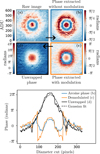 |
Fig. 2 Experimental demonstration of high dynamics phase measurement with the iMZ: reconstruction of the influence function of one of the 140 actuators of the CRAL XAO test bench MEMS deformable mirror (see Sect. 7.2.2 for more details about the experimental setup). Upper panel: pupil plane images of the (a) raw intensity measured on the asymmetric iMZ output, (b) phase retrieved by the arcsine without modulation, (c) phase retrieved by the two-argument arc-tangent with modulation and (d) phase obtained by unwrapping the phase in (c). All phases have been extracted given the calibrated model parameters (see Sect. 5.1). Bottom panel: horizontaL cut of the actuator influence function centered at its peak for the different retrieved phases. at different stages of reconstruction. |
3 Sensitivity of the iMZ
In this section, an expression of the iMZ sensitivity – i.e., how the measurement noise affects the phase estimation – is established in the unmodulated and modulated cases using the model of the data statistics described in Sect. 2.3.1 and the estimators of the phase proposed in Sects. 2.3.2 and 2.4.1. The iMZ sensitivity is compared to that of other WFSs in the limit of a negligible read-out noise (photon counting regime).
3.1 Sensitivity of the iMZ without phase modulation
According to Eq. (12) and assuming that no clamping is necessary, the joint MLE of the sine of the phase is
 (25)
(25)
whose variance can be computed as follows:
 (26)
(26)
since the ouput channels are mutually independent, using  , and finally using Eqs. (11) and (9). The variance of the joint MLE of the phase, ϕ, can be approximated by (Scott 1992)
 (27)
(27)
The same reasoning for the MLE, ϕc , obtained from a given output channel c ∈ {s, a} and given in Eq. (14) yields
 (28)
(28)
It can be noted that
 (29)
(29)
as is expected for optimal estimation from independent sources.
For small phase, ϕ (closed-loop regime), sin ϕ ≈ 0 while cos ϕ ≈ 1 and the variances of the MLEs of the phase simplify to
 (30)
(30)
 (31)
(31)
for c ∈ {s, a}.
In the case of a 50/50 beam splitter (αs = αa = α), the variances of the estimators of a small phase, ϕ, from a single output channel of the iMZ become equivalent for the two outputs:
 (32)
(32)
and simplifies to the following for the joint MLE:
 (33)
(33)
There is thus a gain of 2 in variance compared with the estimation from a single output. We notice that the contribution of the photon noise evolves as 1/N and that of the read-out noise as 1/N2. In the case of negligible read-out noise (high flux condition and low noise detector), the sensitivity is inversely proportional to the ratio α/β2 . This result is consistent with the iMZ contrast expression for each output, equal to the ratio, α/β: the greater the factor, β, of the sine of the phase compared to the offset, α, the higher the sensitivity.
For a 40/60 beam splitter, Fig. 3 plots the variances of the estimated phases as functions of the inward flux and combining or not the two outputs of the iMZ. We can notice a gain of almost two in variance when the phase signal is jointly estimated from both outputs, compared to the separate phase extraction from any single output. The asymmetric output is slightly more sensitive than the symmetric one. This depends on the pinhole size and the beam splitter ρ2/τ2 ratio; here, we used ρ2/τ2 = 40/60. With a 50/50 beam splitter, both outputs would have equal sensitivity as αa = αs in this configuration. The ratio 40/60 is close to the optimal setting (maximized sensitivity) for the λ/D diameter pinhole. It should be noted, however, that this pinhole size does not correspond to the optimum settings, as a larger pinhole (between 1.5 and 2 λ/D) would reduce flux losses due to the pinhole filter, while providing a suitable reference wavefront. This topic is not developed further in this article but will be addressed in future work. We observe in Fig. 3 a good agreement between the theoretical (solid lines) expressions of the variances and the simulated (dashed lines) results, for a flat incident wavefront. These simulations average more than 10 000 independent realizations. This plot shows that a minimum of twenty-eight photons per pixel in the pupil (upstream of the sensor) are needed to achieve phase measurement precision compatible with a Strehl ratio at least equal to 90%. We compare on Fig. 4 the iMZ performances in terms of sensitivity with other WFS used in AO, the SHWFS, the FPyWFS (fixed pyramid WFS) and the Zernike mask.
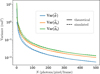 |
Fig. 3 Variances of the iMZ phase estimators (in rad2, logarithmic scale) as a function of N the number of photons per pixel per frame available for measurement for the λ/D pinhole diameter and 40/60 beam splitter. The expressions of the estimators are given in Eqs. (12) and (14). The solid lines plot the theoretical variances, given in Eqs. (30) and (31), for the joint (in blue), symmetric (in green), and asymmetric (in orange) MLEs of the phase. The dashed lines correspond to the simulated results for a null input phase. |
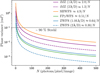 |
Fig. 4 Analytical photon noise variance (in rad2, logarithmic scale) as functions of the number, N, of photons per pixel per frame available for the phase measurement at the entrance of various WFSs: the SHWFS (in orange, Rousset et al. 1987), the unmodulated PYWFS (in green, Chambouleyron et al. 2023), the 1.06 λ/D and 2λ/D dot diameter ZWFS (in blue, Chambouleyron et al. 2023, Haffert et al. 2023) and the iMZ in purple for a λ/D (solid line) and 2λ/D (dashed line) diameter pinhole. |
3.2 Comparison with other WFSs
To compare the theoretical sensitivities of the SHWFS, the FPy-WFS, the ZWFS, and the iMZ, we consider the read-out noise to be negligible. The phase measurement errors are therefore only due to photon noise and, for a fair comparison, we account for photon loss that occur for the different WFSs. The phase variances for the FPyWFS and the ZWFS are, respectively, 0.5/N and 0.7/N, as derived by Chambouleyron et al. (2023), while the SHWFS variance is given in Rousset et al. (1987) for diffraction limited spots. Two pinhole diameters (1 and 2 λ/D) are considered for the iMZ for which the variance of the measured phase is given in Eq. (27) with σron = 0 e−/pixel/frame. Figure 4 plots the variances of the phase measured by the different WFSs as a function of the number N of available photons per pixel per frame in the entrance pupil. We first note that the classical iMZ (λ/D diameter pinhole) is more sensitive than the SHWFS, with σ2SHWFS ≈ 1.8 σi2MZ1. Doubling the pinhole diameter reduces significantly the measured iMZ phase variance by a factor greater than 2. The 2 λ/D iMZ is still less sensitive than the Fourier filtering WFSs, with factor of ≈2 in variance for the FPyWFS and a factor of ≈4 in variance for the ZWFS2. Those results correspond to the ultimate sensitivity of the iMZ WFS, for wavefront distortions close to zero (i.e., in closed-loop operations with small or negligible static non-common path aberrations) and negligible read-out noise. These results also confirm that the iMZ sensitivity to photons is higher by a factor ranging from 1.5 to 3 from the previous estimations derived by Guyon (2005) to deliver the same level of performances.
3.3 Sensitivity of the phase modulated iMZ
In this section, we derive the expression of the variance of the phase measured by the modulated iMZ. For the general case of iMZ data with known perturbations, the MLEs of the sine and cosine of the phase are given in Eq. (18). Noting that the left-hand side matrix, A, given in Eq. (19), is symmetric by construction and that only the right-hand side vector, b, given in Eq. (20), depends on the data, the covariance matrix of the MLEs of the sine and cosine of the phase read as
 (34)
(34)
Considering the linear dependency of b in the data – see Eq. (20) – and since the data pixels and frames are mutually independent, the covariance of b reads as
 (35)
(35)
where the exponent τ denotes the transpose. Now, since  , the covariance of b simplifies to
 (36)
(36)
Combining Eqs. (34) and (36), the covariance matrix of the MLEs of the sine and cosine of the phase is simply given by
 (37)
(37)
The variance of the phase estimator given in Eq. (21) is then approximately given by
![Mathematical equation: \Var\Paren[\big]{\estim{\phi}} &\approx \Vector{\partial\phi/\partial\xi\\\partial\phi/\partial\zeta}\T\cdot \Cov\Paren*{\Vector{\estim{\xi}\\\estim{\zeta}}}\cdot \Vector{\partial\phi/\partial\xi\\\partial\phi/\partial\zeta}\\](/articles/aa/full_html/2025/09/aa53987-25/aa53987-25-eq78.png) (38)
(38)
 (39)
(39)
For a small phase aberration, ϕ, a small perturbation, wk, and negligible read-out noise, the variance of the perturbated data in Eq. (16) is approximately  . Then, for a simple modulation, i.e., wk = ±w and M = 2, in the contribution of a given channel, c, in the left-hand side matrix A – given in Eq. (19) –the off-diagonal terms cancel each other out, while the diagonal terms are equal to
 (40)
(40)
Applying the formula in Eq. (39), the variance of the estimated phase when the two ouput channels of the iMZ are combined is approximately given by
![Mathematical equation: \Var\Paren[\big]{\estim{\phi}} \approx \Paren*{\sum_{c \in \{\Sym,\Asym\}} \frac{N\,\beta_{c}^{2}}{\alpha_{c}}}^{-1}\, \chi(\phi,w),](/articles/aa/full_html/2025/09/aa53987-25/aa53987-25-eq82.png) (41)
(41)
with
 (42)
(42)
When the phase is extracted from a single output channel of the iMZ, its variance is approximately given by
![Mathematical equation: \Var\Paren[\big]{\estim{\phi}_{c}} \approx \frac{\alpha_{c}}{N\,\beta_{c}^{2}}\, \chi(\phi,w).\vspace*{-5pt}](/articles/aa/full_html/2025/09/aa53987-25/aa53987-25-eq84.png) (43)
(43)
For a given phase error, ϕ, the minimal variance is for a perturbation such that
 (44)
(44)
which immediately follows from
 (45)
(45)
and which yields
 (46)
(46)
Finally, in the considered conditions, the minimal variances of the phase estimators for the modulated iMZ are given by
![Mathematical equation: \Var\Paren[\big]{\estim{\phi}} &\underset{\substack{\phi \rightarrow 0\\\sigma_{\RON} \rightarrow 0}}{\approx} \Paren*{\sum_{c} \frac{N\,\beta_{c}^{2}}{\alpha_{c}}}^{-1},](/articles/aa/full_html/2025/09/aa53987-25/aa53987-25-eq88.png) (47)
(47)
![Mathematical equation: \Var\Paren[\big]{\estim{\phi}_{c}} &\underset{\substack{\phi \rightarrow 0\\\sigma_{\RON} \rightarrow 0}}{\approx} \frac{\alpha_{c}}{N\,\beta_{c}^{2}}.](/articles/aa/full_html/2025/09/aa53987-25/aa53987-25-eq89.png) (48)
(48)
For small phase aberrations, negligible read-out noise, and no photon loss between successive detector frames, Eqs. (32) and (33) show that the sensitivity of the modulated iMZ is comparable to that of the unmodulated iMZ. In that respect, the modulation yields no loss compared to the unmodulated case. Equation (44) provides a way to automatically tune the amplitude of the modulation. This naturally leads to use a significant modulation while closing the loop (bootstrap regime) and then to turn off the modulation as the small phase regime is reached (unmodulated regime).
With modulation, the perturbation could for instance be created by alternating positive and negative small waffle patterns to create four localized small intensity spots in the image plan with a very small impact on the HCI sensitivity and that could in addition be used for tip-tilt measurements with coronagraphy (Cantalloube et al. 2019).
4 Chromatic behavior of the iMZ
The previous results were obtained using the approximation of a monochromatic source, i.e., with zero spectral range and infinite coherence length. The monochromatic model faithfully describes the experimental results obtained in the laboratory, with an helium-neon laser source emitting at 632.8 nm, with a spectral width of approximately one picometer, and a coherence length of several tens of centimeters. In this section, the effect of spectral bandwidth broadening on the iMZ signal is studied, using both analytical and simulated results. This study is mandatory to consider the on-sky use of the iMZ because natural guide stars will allow one to access more photons if the measurements are performed in a broad spectral band.
Compared to the monochromatic case in Eqs. (9) and (10) and for a small enough difference between the aberration and the calibration phase owing the pinhole size, the expectation of the signal obtained in the output channel c for a broadband source can be written as
![Mathematical equation: \mathbb{E}\Paren[\big]{d^{\poly}_{c}} &= \int\nolimits_{\Delta\lambda} \frac{\partial N}{\partial\lambda}\, \Brack*{\alpha_{c}(\lambda) + \beta_{c}(\lambda)\,\sin\phi(\lambda)}\, \mathrm{d}\lambda\\](/articles/aa/full_html/2025/09/aa53987-25/aa53987-25-eq90.png) (49)
(49)
 (50)
(50)
with ∆λ the spectral bandwidth, ∂N/∂λ the spectral distribution of photons, ϕ(λ) the chromatic phase, and αc(λ) and βc (λ) the chromatic model parameters. The total number of photons received on average and the mean parameter, αc (λ), are given by
 (51)
(51)
 (52)
(52)
Under the assumptions leading to Eq. (50), ΝΔλ and ᾱc only depend on the spectral distribution of photons, not on the phase aberration. Hence, only the parameter βc is affected by the chromatism of the phase aberration. In order to analyze the effects of the chromatism, the sine of the chromatic phase can be rewritten as
![Mathematical equation: \sin\phi(\lambda) = \sin\phi^{\dag}\,\cos\Paren[\big]{\phi(\lambda) - \phi^{\dag}} + \cos\phi^{\dag}\,\sin\Paren[\big]{\phi(\lambda) - \phi^{\dag}}](/articles/aa/full_html/2025/09/aa53987-25/aa53987-25-eq94.png) (53)
(53)
with  the phase aberration implicitly defined by
![Mathematical equation: \int\nolimits_{\Delta\lambda} \frac{\partial N}{\partial\lambda}\,\beta_{c}(\lambda)\, \sin\Paren[\big]{\phi(\lambda) - \phi^{\dag}}\,\mathrm{d}\lambda = 0.](/articles/aa/full_html/2025/09/aa53987-25/aa53987-25-eq96.png) (54)
(54)
With this particular choice, Eq. (50) becomes
![Mathematical equation: \mathbb{E}\Paren{d^{\poly}_{c}} = N_{\!\Delta\lambda}\, \Paren[\big]{\mean{\alpha}_{c} + \eta^{\dag}\,\mean{\beta}_{c}\,\sin\phi^{\dag}}](/articles/aa/full_html/2025/09/aa53987-25/aa53987-25-eq97.png) (55)
(55)
with
 (56)
(56)
![Mathematical equation: \eta^{\dag} &= \frac{1}{N_{\!\Delta\lambda}\,\mean{\beta}_{c}}\,\int\nolimits_{\Delta\lambda} \frac{\partial N}{\partial\lambda}\,\beta_{c}(\lambda)\, \cos\Paren[\big]{\phi(\lambda) - \phi^{\dag}}\,\mathrm{d}\lambda.](/articles/aa/full_html/2025/09/aa53987-25/aa53987-25-eq99.png) (57)
(57)
Apart from the averaging of the model coefficients and the η† factor, Eq. (55) is very similar to the monochromatic model in Eq. (10). Provided the chromatism of the phase aberration is moderate, i.e., φ(λ) ≈ φ† the cosine can be approximated by the two first terms of its Taylor series to yield
![Mathematical equation: \eta^{\dag} \approx 1 - \frac{1}{2}\,\Avg[\big]{\Paren[\big]{\phi(\lambda) - \phi^{\dag}}^{2}}_{\Delta\lambda}](/articles/aa/full_html/2025/09/aa53987-25/aa53987-25-eq100.png) (58)
(58)
where
![Mathematical equation: \Avg[\big]{\Paren[\big]{\phi(\lambda) - \phi^{\dag}}^{2}}_{\Delta\lambda} = \frac{1}{N_{\!\Delta\lambda}\,\mean{\beta}_{c}}\,\int\nolimits_{\Delta\lambda} \frac{\partial N}{\partial\lambda}\,\beta_{c}(\lambda)\, \Paren[\big]{\phi(\lambda) - \phi^{\dag}}^{2}\,\mathrm{d}\lambda](/articles/aa/full_html/2025/09/aa53987-25/aa53987-25-eq101.png) (59)
(59)
is some measure of the chromatic variance of the phase aberration. For φ(λ) ≈ φ† η† is positive but less than one, which expresses the loss of contrast for a broadband source compared to the monochromatic case with parameters ᾱc and β̄c. This loss of contrast is illustrated by end-to-end (E2E) numerical simulation results in Fig. 5. A light source with a central wavelength λ0 = 1 μm and a spectral range of ∆λ = 400 nm, sampled in 11 wavelengths at 40 nm intervals, is used for the simulation. The sum of the irradiances (intensities) corresponding to each wavelength (without interactions between photons of two distinct wavelengths) is made to simulate the iMZ broadband response. A phase expressed at a wavelength, λ, is computed from the phase expressed at λ0, assuming that the aberration corresponds to an achromatic optical path delay hence, using the following expression:
 (60)
(60)
The phase shifts experienced by the beam during propagation and the pinhole size are also scaled by the wavelengths ratio, λ0 /λ, to take into account spectral dependencies. The effects of spectral bandwidth broadening for an input phase aberration of 250 nm RMS, generated in simulation by pushing the 12 × 12 DM actuators randomly between −400 nm and 400 nm, are shown in Fig. 5.
We note that the broadening of the spectral bandwidth causes a small decrease in the fringe contrast on both iMZ outputs. A relative 19 % drop in contrast is measured on the symmetrical output, and 9 % on the asymmetrical output. This difference is due to the asymmetry of the iMZ dichroic which leads to different βc for its two outputs. The contrast, η†, being inversely proportional to βc, the loss of contrast is higher for the symmetric output than for the asymmetric output. Despite this reduction in visibility, the interference fringes remain clearly visible, and the increase in the spectral bandwidth of the source does not entirely blur the interference signal. The reduction in visibility of the iMZ fringes depends on the spectral bandwidth of the source, but also on the incident aberration. The contrast obtained for Fig. 5 phase aberration with increasing RMS, ranging from 50 to 100 nm RMS, is presented in Table 2. We can note that the larger the RMS of the input aberration on the pupil, the larger the loss in contrast due to the spectral broadening of the source. The observed contrast loss translates into a loss of sensitivity, because it reduces the amplitude of the variations in intensity for the same input aberration. However, widening the spectral bandwidth of the source increases the number of photons received and therefore reduces the photonic phase measurement error, which is inversely proportional to the number of photons received (in variance).
In the broadband case, the model in Eq. (55) is very similar to the nonlinear model given by Eq. (10) for a monochromatic source. Thus the same methods and formulae as before can be used to estimate the phase aberration, ϕ†, by substituting the parameters N, αc, and βc, respectively, by ΝΔλ, ᾱc, and η† β̄c. It must, however, be noted that, although ΝΔλ, ᾱc, and β̄c do not depend on the phase aberration, the loss of contrast η† does depend on the chromatism of the phase aberration, which poses calibration issues. As is shown next, these issues disappear in closed-loop operations when the phase aberrations are small.
For AO systems, aberrations are mostly due to an achromatic variation, δ, in the optical path and the chromatic phase reads as φ(λ) = 2 πδ/λ. For small wavefront distortions, sin φ(λ) ≈ 2πδ/λ and the expectation of the broadband signal in Eq. (50) simplifies to
![Mathematical equation: \mathbb{E}\Paren{d^\poly_{c}} \approx N_{\!\Delta\lambda}\, \Paren[\big]{\mean{\alpha}_{c} + \beta^{\ddag}_{c}\,\phi^{\ddag}},](/articles/aa/full_html/2025/09/aa53987-25/aa53987-25-eq103.png) (61)
(61)
with φ† = 2 πδ/λ‡ the phase at a chosen wavelength, λ‡, and
 (62)
(62)
It may be noted that  and β̄c, in Eq. (56), are different definitions of the average value of βc(λ) in the spectral bandwidth.
In the limit of small aberrations, the signal has the same expression for the monochromatic and broadband cases provided that parameters N, αc, and βc be replaced by ΝΔλ, ᾱc, and  , respectively. As a consequence, the expressions of the phase estimators and of their variances are readily given by substituting these parameters in Eqs. (12), (14), (30), and (31). Below, we give the expressions of the variances of the estimators of the phase, taking into account the spectral bandwidth:
 (63)
(63)
 (64)
(64)
 (65)
(65)
 (66)
(66)
for c ∈ {s, a} and where  is the number of received photons on average in the spectral bandwidth, ∆λ. The parameters ᾱc and
  are the weighted means of αc (λ) and βc (λ) over the spectral bandwidth (with different weights) and should not depend too much on ∆λ. Hence, in the small aberration regime, increasing the spectral bandwidth reduces the variances of the estimators. Photonic phase variance errors based on Eq. (64) for 50 nm to 100 nm RMS aberrations are reported in Table 3. A similar result can be obtained by calculating the phase variance from the residual pupil measurements by accounting for the collected photons in both cases assuming a flat source spectrum and after adding the associated photon noise to the simulation. To perform this calculation, the wavefront is reconstructed using the broadband model parameters
  defined by
 (67)
(67)
 (68)
(68)
 (69)
(69)
The photonic phase measurement error obtained for the same input aberrations than Table 3 is shown in Table 4. There is a significant decrease in the phase photonic measurement error for the polychromatic case almost equal to the root of the flux ratio between the two sources ( ). If the decrease in contrast had no impact on the phase measurement error, the ratio between the two cases should be exactly equal to
  , since this error evolves in inverse proportion to the root of the number of received photons. In fact, the small contrast decreases from Table 2 implies that β decreases and α increases, thus reducing slightly the sensitivity (which evolves as α/β2). As expected the phase measurement error also increases with the RMS of the aberrations to be measured. As a consequence, this effect would be negligible in closed-loop regime. As an example, for the smallest wavefront deformations simulated in this section (see Table 4), the effect of chromatism is negligible, and the main effect of spectral band broadening is the reduction in phase photonic measurement error due to the gain in photons available for measurement, as illustrated on Fig. 6 residual maps.
In conclusion, for small wavefront distortions (closed-loop XAO), the chromatic effects linked to increasing the spectral bandwidth (∆λ = 400 nm tested here) remain small compared to the gain in terms of photons received. However, spectral band broadening could become a concern in the case of larger wavefront distortions (several multiples of the wavelength), leading to a significant reduction in visibility. Dedicated simulations in this regime, corresponding for instance to the XAO initial bootstrapping stage for strong turbulence compensation, would be required to simulate the effects of spectral bandwidth broadening on iMZ sensitivity.
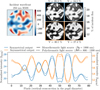 |
Fig. 5 Noise-free simulation of iMZ response for a monochromatic (1000 nm) and broadband (800–1200 nm uniformly cut into 11 intervals 40 nm wide) light source, for an input aberration of 250 nm RMS (top left). The flux is 10 photons/pixel for each spectral interval (hence 11 times more photons in total for the broadband source compared to the monochromatic one). The interferograms’ intensities are displayed as a percentage of the incident flux. Top left: random incident wavefront phase produced by the DM actuators. Top right: interferograms obtained for each iMZ output (symmetrical in blue, asymmetrical in orange), monochromatic (solid line) and polychromatic (dotted line). Bottom: vertical section through the pupil diameter of the four interferograms. The visibility was calculated as V = (Imax - Imin)/(Imax + Imin), with Imin and Imax the minimal and maximal intensities measured in the image of the pupil. |
Comparison between monochromatic and broadband contrasts.
Photonic phase measurement error (standard deviation in nanometers) calculated analytically.
Photonic phase measurement error (in nanometers) calculated from the simulated residual standard deviation.
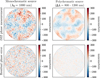 |
Fig. 6 Simulation of the iMZ phase measurements for a monochromatic (left) and polychromatic (right) light source, for the 50 nm RMS incident aberration (wavefront from Fig. 5 divided by 5). |
5 The iMZ calibration procedure
The method we propose for the iMZ calibration consists in estimating the model parameters to reconstruct directly the phase from the intensity signal measured on the detector. The objective of calibration is to estimate the terms N αa, N αs, N β, and the phase, ϕ. The method described here allows one to disentangle the phase signal (ϕ) from the model parameters (N αa, N αs, and N β). Once these latter parameters are calibrated, the phase can be computed by simply applying the estimation method developed in Sect. 2.3.2.
5.1 Maximum likelihood calibration
The proposed calibration method is based on the maximum likelihood approach used in Sect. 2.4.1 to derive the estimator of the phase in the presence of a known modulation but generalized to also estimate the model parameters. To simplify the developments of the method, we assumed that the calibration images were acquired with the same exposure time as for the images acquired for measuring the phase. This amounts to discarding the 1/M factor in the model given in Eq. (15). The expectation of a given pixel in the k-th calibration image in output channel c can then be expanded and rewritten as follows:
 (70)
(70)
with wk the k-th applied perturbation, x1 = N αs, x2 = N αa, x3 = Nβ sin φ, x4 = Nβ cos φ, εc = 1 (resp. εc = 2), and ςc = −1 (resp. ςc = +1) for the symmetric (resp. asymmetric) output (c = s, resp. c = a). Clearly, the calibration data model in Eq. (70) is linear in the four unknowns x = (x1, x2, x3, x4) per pixel. If the data for a given pixel in the two output channels of a sequence of M calibration images are collected in a vector, y ∈ R2M, then y ≈ H · x, with H ∈ R(2 M)×4 a matrix built according to Eq. (70) and where the ≈ sign accounts for the measurement noise. Then, assuming as in Sections 2.3.2 and 2.4.1 that the data noise is approximately Gaussian, a maximum likelihood estimator (MLE) for x is given by
 (71)
(71)
 (72)
(72)
where W = Cov(y)−1 is the precision matrix of y. Since the noise is independent, W is a diagonal matrix whose diagonal entries are the reciprocal of the corresponding data variances. Finally, inverting the relationship between x and the parameters of interest yields the following MLEs of the model parameters and of the phase:
 (73)
(73)
 (74)
(74)
 (75)
(75)
![Mathematical equation: \estim{\phi} &= \mathtt{atan2}\Paren[\big]{\estim{x}_{3}^{2},\estim{x}_{4}^{2}}.](/articles/aa/full_html/2025/09/aa53987-25/aa53987-25-eq125.png) (76)
(76)
The method can also be applied to the pixel values for a single output channel (symmetric or asymmetric) to only calibrate the three model parameters for this output.
The proposed calibration procedure makes no other assumption than the model presented in Eq. (9), it is general and applicable for large aberrations. The closed-form expression in Eqs. (73), (74), (75) and (76) can be carried out independently for all pixels of the pupil to directly give the calibration parameters. If the interval of values of the aberrated phase ϕ is larger than 2 π, an additional unwrapping procedure must be applied, as described in Sect. 2.4.2.
The efficiency of this calibration method strongly depends on the introduced phase modulation which must map the phase range [-π, π]. Our tests performed in simulation and experimentally on the XAO bench have shown that the phase modulations that give the best calibration results are given by w ≈ (−0.8 π, −0.4 π, 0, +0.4 π, +0.8 π). These phase offsets uniformly map the sine and the cosine function between -π and π. A minimum of four steps are necessary to have a unique solution to Eq. (71) which is a robust estimator of the calibration model parameters.
The shape of the phase modulation injected to calibrate the iMZ is an important parameter. The proposed calibration relies on the knowledge of the phase modulation w and the simpler the modulation pattern the easier it is to know precisely the modulation. However, a global piston is unseen by the iMZ as is the case for all WFSs. As a compromise, we found that, in practice, a simple procedure is to generate local phase pistons in small patches by activating groups of 4 × 4 contiguous actuators of the DM used for the calibration. For each patch, several amplitudes of perturbations are produced to calibrate the model parameters in the patch. This process is repeated so as to map the entire pupil. This method has been successfully tested by simulation and experimentally. Examples of experimental results of the iMZ calibration using its asymmetric output using different phase offsets are shown in Fig. 7.
The phase modulation used to perform the calibration experimentally is generated with a 12 × 12 Micro Electro Mechanical Systems (MEMS) DM. The pupil is mapped with 4 × 4 contiguous actuators that are jointly pushed or pulled to estimate the calibration parameter in square patches one-fifth the pupil diameter. We first notice in Fig. 7 that sampling effects are hardly discernible in the maps of the three calibration parameters  ,
,  , and ϕ̂. Pinhole filtering effect is visible in
  and
and  maps, with an attenuation of the intensity at the edges of the pupil. One of the advantages of the calibration method lies in the joint estimation of the phase (ϕ) and of the other model parameters (here N αa and N β) whose contributions are well disentangled. The three different phase offsets applied during the calibration are indeed recovered as a change of phase and not as a change in intensity, as
  ,
,  remain constant in the three cases. However, we can notice that for the highest phase offsets (random pushes, third column of Fig. 7) some of the phase structures are present in the intensity maps
  , i.e., extracted as intensity and not phase variations. This effect is mainly due to the approximation that the model parameters αc and β are phase independent, while they are actually functions of Ĩ the intensity distribution after filtering by the pinhole whose effect depends on the phase. In the next section, we show how to mitigate this effect by taking into account the intensity variations in the model caused by the incident phase.
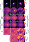 |
Fig. 7 Experimental result of iMZ signal calibration using the asymmetric output, with three different phase offsets applied to the DM in addition to the phase diversity steps required to perform the calibration. First row: peak-to-valley ≈140 nm, σ2 ≈ 0.06 rad2. Second row: peak-to-valley ≈ 250 nm, σ2 ≈ 0.1 rad2. Third row: peak-to-valley ≈310 nm, σ2 ≈ 0.5 rad2. The first line correspond to raw focal plan images produced behind the pinhole with the three DM settings. The second line shows the pupil plane signal of the asymmetric output. Lines 3 to 5 show the measured calibration parameters N αa, Nβ, and ϕ estimated with weighted least mean square method for these three DM settings. The DM shape is shown for comparison on the last line. |
5.2 Model parameters phase dependency
Looking at Eqs. (7a)–(7c), the model parameters αa, αs, and β are functions of the images I and Ĩ of the pupil. The unfiltered image, I, only depends on the amplitude of the field in the pupil and is thus independent of the phase, ϕ. On the contrary, Ĩ depends on the shape of the PSF imaged on the pinhole and this shape strongly depends on the phase. Hence, Ĩ and, as a consequence, the model parameters depend on the phase ϕ. This dependency is implicitly neglected in the calibration method presented in Sect. 5.1. Such an approximation is valid for small phase aberrations but, for stronger aberrations, yields a bias in the estimation of αa, αs, and β which, in turn, impacts the estimation of the phase ϕ.
To study the impact of the phase, ϕ, we rewrote the model parameters in Eqs. (7a)–(7c) as
 (77a)
(77a)
 (77b)
(77b)
 (77c)
(77c)
with γ = (Ĩ/I)1/2, which can be seen as the amplitude of the filtered image relative to that of the unfiltered one. The variations in the iMZ model parameters (αa, αs, and β) with γ are plotted on Fig. 8a. For small phase aberrations (e.g., closed-loop regime), the relative filtered amplitude, γ, only depends on the size of the pinhole, which determines the fraction of inward photons that are reflected by the pinhole. For a flat wavefront, γ is a pixel-wise function whose shape is shown for different pinhole sizes by Fig. 8b. For small pinhole diameters, the filtered amplitude is relatively flat across the pupil. For example, γ ≈ 0.46 for a λ/D diameter pinhole. For diameters up to 2 λ/D, the relative filtered amplitude has a more pronounced bell-shaped profile as the pinhole size increases. For a 4 λ/D diameter pinhole, the profile shows oscillations. For stronger phase aberrations, ϕ, the relative filtered amplitude, γ, also depends of the phase. This is illustrated by Fig. 8c where the mean value of γ is plotted for a phase aberration taking values from -π/2 to π/2 and whose shape is one of the fifty first Zernike modes. We note an important decrease in ⟨γ⟩ for the first Zernike modes; this loss is maximal for a defocus (Z4), with only 20% of the incident photons reflected on the λ/D pinhole, compared to 46% for a piston (Z1). For the considered aberrations, the model parameters strongly depend on the shape of the aberration: between a piston and a defocus, the parameter β changes by more than a factor of 2 while the relative variations are, respectively, 1.4 and 1.2 for αs and αa. As a consequence, the model parameters calibrated on a flat wavefront cannot be used without adjustments to reconstruct large aberrations.
For a small pinhole size, the relative filtered amplitude, γ, remains very smooth and, compared to a flat wavefront, a distorted wavefront mostly reduces the flux reflected by the pinhole. We propose to exploit this simple behavior to account for the incidence of a phase distortion by a simple loss factor, η(φ) ∈ [0,1], such that
 (78)
(78)
where γflat is the relative filtered amplitude calibrated for a flat wavefront, while γ is the relative filtered amplitude for the actual phase distortion, ϕ. Since the pinhole is not fully reflective (its transmission is about 3-5%), the loss factor, η(φ), can be measured experimentally with the iMZ by using the light distribution outgoing behind the pinhole (coronagraphic output):
 (79)
(79)
with Iback(0) the central value of the PSF re-imaged behind the pinhole and Iback,flat(0) the same quantity for a flat wavefront. To improve this estimator, the value of Iback averaged over a small central region may be used instead of the central value. Iback is proportional to the coronagraphic PSF, which is an hybrid PSF whose legs are fully transmitted and whose central core is attenuated by the pinhole.
Combining the approximation in Eq. (78) that holds for a small pinhole size and Eqs. (77a)–(77c), the expressions of the iMZ model parameters can be modified as follows:
 (80a)
(80a)
 (80b)
(80b)
where αflat,0,c, αflat,1,c, and βflat for c ∈ {s, a} are calibrated on the iMZ for a flat wavefront. The term αflat,0,c corresponds to the image at the output channel c in the absence of interferences (i.e., when γ = 0) and can thus be calibrated by measuring this image when the input beam is tilted so as to not reflect on the pinhole. The term αflat,1,c can then be deduced by subtracting αflat,0,c from the calibrated αc for a flat wavefront and when the beam is normally aligned with the pinhole.
The same phase estimators as those proposed in the previous sections can be used with the model parameters modified according to Eqs. (80a)–(80b) to simply account for the change of model parameters induced by the phase aberration to be measured. This correction improves the estimation of the phase for aberrations larger than one wavelength in peak-to-valley and implies to monitor the transmitted intensity behind the pinhole. We use this compensation method whenever needed in the following E2E simulations and experimental phase measurements.
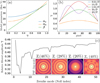 |
Fig. 8 Variations in the model parameters with the filtered relative amplitude, γ. (a) The parameters αs, αa, and β (in percent of the incident flux) as functions of γ, see Eqs. (77a)-(77c). (b) Radial cut of γ for a flat wavefront and pinhole diameters from 0.5 to 4 λ/D. (c) Mean value of γ in the pupil for a phase aberration with taking values from -π/2 to π/2 and whose shape is one of the fifty first Zernike modes, for a λ/D pinhole. Below the curve we show the PSFs in logarithmic scale for Z1, Z2, Z4, and Z25. The pinhole diameter is overlaid with a black circle. The percentages indicated for each Zernike mode corresponds to the PSF energy encircled within the pinhole. |
6 iMZ closed-loop performances
In this section we quantify the iMZ performances in closed-loop regime by using E2E simulation for different turbulence regimes and flux conditions. First, the performances are estimated with the iMZ used as a first stage WFS with only tip-tilt pre-correction, for a circular 8-meter pupil without segmentation, for two seeing conditions corresponding to good (0.4 arcsecond) and median conditions (0.7 arcsecond). In the second part we will evaluate the performances of the iMZ when used as a second stage WFS in the conditions of SAXO+ (Sphere Adaptive-optics for eXoplanet Observation+), the double stage XAO system foreseen to enhanced the performances of VLT/SPHERE (Spectro-Polarimetric High-contrast Exoplanet REsearch instrument) (Beuzit et al. 2019), SPHERE+ (Boccaletti et al. 2020). Finally, a brief overview of the iMZ performances in closed loop with the ELT segmented pupil is presented.
6.1 Single-stage XAO closed-loop performances with 8m telescopes
A summary of the parameters used for these simulations is presented in Table 5. The one second turbulent phase sequence (1000 frames) used for the two considered seeing cases (0.4 and 0.7 arcsecond) was generated with the AO simulation tool COMPASS (Ferreira et al. 2018) developed for the SAXO+ (Goulas et al. 2024).
A perfect tip-tilt pre-correction is assumed here. Thanks to the iMZ configuration, the tip-tilt closed loop can be driven by using the spare photons from the spatial filtering to create the reference wave (coronagraphic output, see Fig. 1). A perfect DM correction is assumed in the following, i.e., the command equals the WFS measurement and no fitting error will be present in correction residuals. We thus consider the corrector to be a perfect DM with an infinite number of actuators. A 1.5 λ/D pinhole diameter iMZ is used to measure the residual phase aberrations.
We use a simple integrator with a gain g = 0.3 for the control law and assume a delay of one frame. At iteration k of the control loop, the DM command reads
 (81)
(81)
where D+ is the pseudo-inverse of the DM influence function matrix D and ϕ̂k is the estimated phase given by the average of the phases measured by the two iMZ outputs and using the calibration parameters estimated with the method presented in Sect. 5. During the closed-loop sequence, if the command stops evolving and if there are some outlier pixels/subapertures, a nearest neighbor averaging is applied to fix these outliers.
Simulation parameters used for closed-loop simulation for a single-stage XAO using the iMZ.
6.1.1 Simulation case: 0.4 arcsecond seeing
This first case corresponds to very good seeing conditions, with a Fried parameter r0 = 26 cm (74 cm at 1.2 μm) and a turbulence coherence time τ0 = 5.3 ms. The evolution of the residual phase variance over the pupil for one second of turbulence and guide star magnitudes ranging from m = 5 to m = 13 is presented in Fig. 9. The corresponding number of photons per pixel/subaperture per frame N at the iMZ entrance ranges from 680 to 0.4, respectively. For these seeing conditions, the phase is measured by the iMZ without modulation or flux adjustment, because the aberrations amplitude remains relatively small and within the iMZ dynamic range.
We notice that the correction converges to high Strehl ratios for 8 out of the 9 simulated cases presented, with Strehl ratio of 90% or better for magnitudes of 9 and below. The case with the faintest guide star magnitude (m = 13) and the lowest number of photon per frame per pixel (N = 0.4) is unstable and is the only one that does not reach a Strehl ratio of 90%. For all other cases, the phase variance residuals over the pupil varies from 0.03 rad2 (SR ≈ 97% at 1.2 μm) for N = 680 pho-tons/pixel/frame to 0.5 rad2 (SR ≈ 65% at 1.2 μm) for N = 1.1 photons/pixel/frame. The plateau observed for bright guide stars (i.e., magnitudes less than 7) on the simulated phase variance residual curves as function of N shows that the phase residual errors are dominated by temporal error (and calibration bias) and not by the photon noise. For magnitudes greater or equal 7, the simulation curves match almost perfectly the photonic residual phase variance curve, evolving as 1.5/N for the 1.5 λ/D pinhole diameter (and a 40/60 beam splitter). The intensity, command and residual maps presented in Fig. 10 shows the evolution of the correction for the magnitude m = 7.
At the starting of the loop, it can be seen in Fig. 10 that the contrast of the iMZ interferogram is very low. This is due to the small amount of flux reflected on the pinhole (with a 5% Strehl) resulting in an important imbalance between the reference arm and the signal arm of the iMZ (hence, βc ≪ αc). At the 10th AO loop iteration, the phase correction reaching 34% Strehl, the contrast of the iMZ interferogram has improved, highlighting wrapped regions of phase residuals. Under these good seeing conditions, the phase is progressively unwrapped thanks to the averaging of outliers but would have required modulation and an unwrapping algorithm under more difficult turbulence conditions, as shown in the next section. These simulations demonstrate the high performance of the iMZ WFS reaching 95% Strehl for guide stars brighter than 8th magnitude. For these cases, the simulations demonstrate that the phase residual errors are most likely dominated by the temporal delay and not by the iMZ itself.
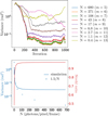 |
Fig. 9 Closed-loop results with the iMZ on 1 second of turbulence, for 0.4 arcsecond seeing, with tip-tilt pre-correction. Upper panel: evolution of the residual phase variance (rad2) during 1000 iterations of correction at 1 kHz for different flux conditions (magnitude 5 ≤ m ≤ 14). Lower panel: residual phase variance (rad2) and Strehl ratio (averaged over the last 500 iterations) as a function of the number N of inward pho-tons/pixel/frame. The blue crosses indicates the photon noise limit of the iMZ (1.5/N) according to the theoretical variance in Sect. 3. |
6.1.2 Simulation case: 0.7 arcsecond seeing
This second case corresponds to good seeing conditions, with a Fried parameter of r0 = 15 cm (42 cm at 1.2 μm) and a turbulence coherence time of τ0 = 5.8 ms. The residual phase variance evolution over the pupil for one second of turbulence and guide star magnitudes ranging from m = 5 to 13 is presented in Fig. 11. The results are plotted without (solid line) and with (dashed line) modulation and processing by a phase unwrapping algorithm processing. This latter strategy, presented in Sect. 2.4, requires one to slow down the loop by a factor of 2, because two images are required to calculate the atan2 of the phase. For these cases, the phase modulation is introduced by a waffle pattern, with a peak-to-valley phase amplitude of 1 radian (200 nm). The calibration parameters are adjusted with a gain according to Eqs. (80a) and (80b) to compensate for the important PSF widening on the iMZ pinhole.
Figure 11 shows that the correction converges to Strehl ratios higher than 90% for four out of the nine simulated cases presented corresponding to the brightest guide stars. We can notice that, in these seeing conditions, low phase variance residuals are only obtained with modulation (and unwrapping) and for the highest magnitudes (m = 5,6,7,8). The cases with guide star magnitudes fainter than 8 do not bootstrap to reach very good AO corrections when using modulation and unwrapping but still show Strehl improvement above 60% for magnitude brighter than 11. This can be explained by the fact that the phase modulation needs twice as many photons as the non modulated regime to be as efficient. One solution which was not investigated would be to slow down the loop further to compensate for the lack of photons at least in the bootstrapping stage.
Figure 12 shows the temporal evolution of the residual phase and of the corresponding PSF for an 8th magnitude guide star without (upper panel) and with phase modulation (lower panel). Without modulation and to control the AO, the phase is estimated by taking the arcsine of the clamped iMZ data, see Eq. (14), while, with modulation, the phase is estimated by the two-argument arctangent function, see Eq. (24), followed by phase unwrapping (see Sect. 2.4.2). At the loop initialization, the Strehl ratio is very low in both cases due to the strength of the turbulence. After 1000 AO loop iterations, the Strehl ratio reaches a stable level better than 80% in both cases. Yet, the phase residuals are much worse in the unmodulated case than in the modulated one (with respective standard deviations of 2.9 rad and 0.4 rad). As can be seen in the upper-left phase map, the strong residual errors in the former case are mainly due to 2 k π discontinuities to which the PSF at the same wavelength is insensitive to. These 2 kπ errors could have been removed by applying phase unwrapping. However, the arcsine function have other degeneracies than the modulo 2 π one and this explains that the Strehl ratio of the PSF at the same wavelength is slightly worse in the unmodulated case than in the modulated one. The PSF at the same wavelength being that of the beam on the pinhole, having a high Strehl ratio is important for the performances of the iMZ. For scientific observations at a different wavelength, the modulo 2 π phase errors would however result in a very bad Strehl ratio. Phase modulation combined with phase unwrapping completely avoids these phase wrapping issues and should be the method of choice. The phase unwrapping stage is the most time consuming operation but it is already applicable with current computers3 for AO systems up to the size of PCS/ELT with 200 × 200 degrees of freedom at a few kilohertz. The only drawback is that, due to the reduced exposure time, the S/N of the data is divided by  and it takes more AO loop iterations (during boostraping) to reach a high correction quality compared to the unmodulated iMZ.
The simulation results presented here show the great sensitivity of the iMZ WFS to measure turbulence in good seeing conditions, with 90% Strehl ratio for guide stars brighter than 9 magnitude for 0.4 arcsecond seeing and for magnitudes lower than 8 for the 0.7 arcsecond seeing. The AO loop driven by the iMZ up to star as faint as 11 or 12 (best seeing) leads to Strehl ratios above 80% for good seeing conditions and from 60% for median turbulence. As the turbulence strength increases, the residual is constrained by the unwrapping error which could be addressed by slowing down the AO loop. In the view of theses very good results, the iMZ seems even better fitted for second stage phase measurements on lower amplitude phase residuals from a first stage AO correction. This will be the topic of the next section.
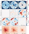 |
Fig. 10 Single-stage closed-loop results obtained with the iMZ using 1 second of evolving turbulence, for 0.4 arcsecond seeing, with tip-tilt pre-correction. Asymmetric iMZ output intensity (first row), measures phase command (second row), residual phase maps (third row) and short exposure PSF (fourth row) for a magnitude 7 guide star (N = 108 photons/pixel/frame). The piston has been removed from both phase commands and phase residual maps. |
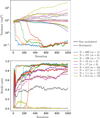 |
Fig. 11 Closed-loop result with the iMZ on 1 second of turbulence, for 0.7 arcsecond seeing, with tip-tilt pre-correction. Upper panel: residual phase variance (rad2) evolution over 1000 iterations of correction at 1 kHz for different flux conditions (m ∈ [5...13], without (solid line) and with modulation + unwrapping (dashed line). Lower panel: associated Strehl ratio estimated at 1.2 µm. |
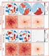 |
Fig. 12 Closed-loop results with the iMZ on 1 second of turbulence, for 0.7 arcsecond seeing, with tip-tilt pre-correction, without (upper) and with phase modulation (lower). Residual phase error (1st row) and short exposure PSF (2th row) for a magnitude 8 (N = 43 photons/pixel/frame). The piston has been filtered out from the residual maps. |
6.2 XAO closed-loop performances with the iMZ as a second stage WFS for SAXO+ conditions
The contrast performance of current XAO systems can be improved by adding a second AO correction stage featuring its own WFS, deformable mirror, and real-time controller. In particular adding a second stage operating at a higher frequency than the first stage is a solution that has been proposed to reduce the temporal error on the 8-meter class telescopes AO systems (Cerpa-Urra et al. 2022; Nousiainen et al. 2024) or for PCS on the ELT (Kasper et al. 2021). In this section, we use E2E numerical simulations to evaluate the performance of an iMZ based second stage XAO. We focus on the SAXO+ conditions a second stage scheme proposed for the upgrade of SAXO, the AO system of SPHERE at the ESO’s Very Large Telescope where the iMZ is replacing the Pyramid as a second stage WFS. The current system, SAXO, includes a visible Shack–Hartmann WFS. We consider fairly difficult SAXO+ conditions where the turbulence is corrected by the 1st stage, equipped with a 40 × 40 Shack-Hartmann and a 41 × 41 DM correcting up to 800 modes (Karhunen–Loève modes). Second-stage correction is provided by a perfect DM, as described in the previous section. The loop configuration is detailed in Fig. 13. For this simulation, a median seeing is considered with r0 = 15 cm and τ0 = 4.6 ms. The 1st and 2nd frequencies are, respectively, set at 150 Hz and 1 kHz, i.e., 3 photons/pixel/frame for the iMZ and 5 photons/pixel/frame for the Shack-Hartmann (≈ magnitude 10 in J band). In these conditions, the low amplitude of the first-stage residuals is such that the iMZ can be used without phase modulation nor flux adjustment.
The closed-loop performances of the iMZ second stage during the first second are presented on Fig. 14. The upper graph displays the temporal evolution of the phase variance of the second stage (blue line) compared to that of the first stage (black line). As shown by the upper graph of Fig. 14, the temporal oscillations produced by the first stage, because the command is applied at a slower rate, result in periodic Strehl oscillations of the order of 5% after the second stage correction. This could be counteracted by optimizing the gain and the control law as proposed by Galland et al. (2023). Apart from these 1st stage oscillations, the correction remains relatively stable and an average Strehl ratio of 87% is obtained over the last 500 iterations, representing an improvement by more than a factor of 3 compared to the Strehl ratio of 27% achieved by the first stage alone. The results simulated here are comparable to those expected with the Pyramid WFS on SAXO+ (Schreiber et al. 2023).
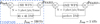 |
Fig. 13 Schematic representation of a second stage with an iMZ WFS, in cascade with the current SAXO AO system, to simulate SAXO+. The first stage is simulated by COMPASS, to generate realistic first-stage residuals. |
7 iMZ wavefront measurements with the ELT
In this section, we simulate the iMZ performances in closed loop with the ELT pupil instead of the 8-meter full circular pupil used in the previous sections. We first consider perfect co-phasing between the different segments with the hypothesis of a monolithic primary mirror. The ELT pupil is formed of six fragments created by the projection of the telescope spider vanes, creating discontinuities in the pupil, and blind areas for wavefront sensing. The fragmentation of the pupil is particularly important in the case of giant telescopes, due to the large thickness of the spider vanes (50 cm for the ELT), which must support a secondary mirror weighting several tons (3.5 tons for the ELT). In such a configuration when the AO is used, differential piston effects can appear (Bertrou-Cantou et al. 2022; Levraud et al. 2024), due to the difficulty of most WFSs (sensitive to the phase gradient) to measure the phase in presence of discontinuities. Low wind effect also contributes to the apparition of similar aberrations, and should be particularly strong in the case of the ELT due to the thickness of the spider vanes.
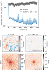 |
Fig. 14 Median seeing SAXO+ simulation with the iMZ as a second stage WFS. The upper graph shows the evolution of phase residual variance (in logarithmic scale) over 1000 correction iterations (loop frequency = 1 kHz) for N = 3 photons/pixel/frame (blue curve). The evolution of phase residual variance after SAXO is overplotted in black (loop frequency = 150 Hz for N = 5 photons/pixel/frame). The lower pictures show residual phase maps and short-exposure focal plane images (log scale) at the beginning and at the end of the one second sequence. |
7.1 Sensing the low wind effect on the ELT
We first simulated the iMZ response to a 500 ms low wind phase sequence generated from a physical toy model for the SCAO simulations of the METIS instrument (Feldt et al. 2024), provided by Martins et al. (2022), with a wind speed of 1 m/s. In this case the evolution of aberrations is quasi-static, with temporal characteristics of the low wind effect (LWE) evolution time greater than the sequence duration used here ≈2 s as measured by Milli et al. (2018) on the VLT. The closed-loop simulations results with the iMZ and perfect correction (perfect DM) are presented Fig. 15.
In this configuration the phase is measured without temporal phase modulation, as the amplitude of LWE screens is relatively low, except near the spider vanes where aberrations can reach ≈ 3 μm. The upper part of Fig. 15 demonstrates the efficiency of the iMZ measurements with Strehl ratio above >90% after 10 iterations. The lower part of the Figure shows that at t = 500 ms (and even before this iteration) most of the structures present on the initial LWE screen have been correctly measured by the iMZ. The phase variance after 500 iterations is less than 0.1 rad2 (SR > 90%). On the residual phase map, a few uncorrected pixels remain in the vicinity of the spider vanes, and they correspond to the highest pixel phase values of the initial LWE screen (2–3 µm), which the iMZ was unable to measure precisely because they are outside its dynamical range. The phase smoothing used to ensure loop convergence is also responsible for small residual structures around the spider vanes. Despite these phase measurement imperfections, the iMZ does improve significantly the image quality, with an average Strehl over the last 100 iterations of over 96% (compared with 41% at the start of the loop) as shown on the Fig. 15 PSF’s. Those preliminary results, obtained with a large number of photons per pixel (equivalent magnitude m = 5, for a pupil sampled over 200 × 200 pixels), shows the iMZ’s potential for LWE measurement for bright guide stars but cannot be easily transposed to lower flux conditions, because phase smoothing performances depend on the photon noise. Nevertheless these LWE aberrations are slowly evolving aberrations that could be measured at smaller temporal frequency (or by combining fast measurements) to decrease photon noise. The low flux LWE measurement performances is beyond the scope of this paper and shall be addressed by dedicated simulations in a separate paper.
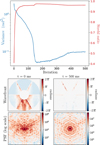 |
Fig. 15 E2E simulation of the iMZ response in closed-loop using a 500 ms sequence (quasi-static) of LWE for the ELT pupil. The upper graph shows the evolution of the phase variance (rad2 ) with time and the associated Strehl ratio during the 500 iterations of AO closed-loop correction with iMZ wavefront sensing. Lower images show the iMZ phase maps at the beginning and at the end of the sequence and the corresponding PSFs. |
7.2 XAO performances on the ELT
7.2.1 E2E simulations of the XAO performances on the ELT
The iMZ response to time evolving atmospheric turbulence has been simulated numerically using the 40-meter ELT pupil. Several sequences of one second of turbulence have been generated with the python tool HCIPy (Por et al. 2018), with r0 = 15 cm (42 cm at 1.2 µm) and L0 = 25 m. The simulation parameters are similar to the previous 8-meter pupil conditions, with a loop running at 1 kHz, one frame of delay, a perfect correction (perfect DM with an infinite number of actuators), tip-tilt filtered out and a simple integrator controller with a gain g = 0.3. In these simulations, the phase is measured using temporal modulation with unwrapping algorithm and flux adjustment of the calibration parameters, that are needed to close the loop in this turbulent regime with a 40-meter telescope pupil. We consider only a bright guide star case (m = 5, i.e., 680 pho-tons/pixel/frame) and iMZ wavefront sensing at 1.2 µm for a good seeing of 0.4 arcseconds. The results of the closed-loop XAO corrections, on a sample of ten one-second sequences of turbulence, are presented on Fig. 16. In four cases out of ten, the loop converges with a residual variance of less than 0.1 rad2 . In three cases out of ten, the loop fails to catch the turbulence and the correction diverges. For the remaining three cases, the loop converges, but one of the six ELT fragments (petal) is shifted in phase compared to the other five, resulting in a differential piston aberration. The difference between the two phase levels is 2π radians, making this aberration invisible to the iMZ WFS. However, at 1.2 µm, the image quality is little affected by this aberration, with a loss of only 0.3% of Strehl compared with the best cases. A Strehl higher than 98% is obtained for seven out of ten cases at 1.2 µm (fitting error not taken into account). The differential piston error obtained in three of the ten cases occurs during the phase unwrapping stage, due to the absence of information under the telescope spider vanes (pixels set to zero) when calculating the Laplacian. This type of aberration does not appear in the small-phase regime, when the control is estimated by inverting the arcsine model. Introducing priors about the turbulence statistics (Thiébaut & Tallon 2010) is a possible way of avoiding the appearance of such patterns but is beyond the scope of this paper. In any case, such island effects or even cophasing errors could be measured and corrected by using spectral diversity for the wavefront sensing. As a conclusion, for very good seeing, the iMZ demonstrates promising performances for handling turbulence in XAO with the ELT but optimizing the bootstrapping phase would be key to enabling its use as a singlestage WFS. Similarly to the VLT case, a second stage iMZ based XAO system for the ELT should deliver very high performances.
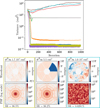 |
Fig. 16 Simulation of the iMZ response with the ELT pupil in closed-loop to ten different atmospheric turbulence sequences corresponding to very good seeing (0.4 arcseconds) and flux conditions (m = 5). Upper part: evolution of the residual phase variance for one second of turbulence, generated with HCIPy (Por et al. 2018). Each of the ten curves correspond to a different turbulence sequence with r0 = 15 cm (42 cm at 1.2 µm) and L0 = 25 m. Bottom part: residual phase maps and corresponding PSFs at the last iteration for three of the ten sequences, representing three typical cases. |
7.2.2 Experimental laboratory validation of the iMZ performances for XAO on the VLT/ELT pupils
In previous sections, we have demonstrated using E2E simulations the iMZ closed-loop performances for handling turbulence in XAO mode or other quasi-static aberrations for ELT and VLT pupils. In this section, closed-loop experimental results obtained with the iMZ on the XAO test bench at CRAL (see Fig. 17) are presented. CRAL’s XAO bench has been developed with the aim of testing different HCI concepts at the ELT scale (Delacroix et al. 2015; Loupias et al. 2016). We will describe the results obtained experimentally for the ELT but also for the VLT pupil.
The light source on the bench is a 632 nm helium-neon laser, the corrector is a 12 × 12 MEMS DM, and wavefront sensing is performed by the iMZ. The DM characteristics are summarized in Table 6. The two pupil images of the iMZ output are imaged on a CMOS detector (Andor Neo), with more than 1000 pixels across the pupil diameter. The filtered flux behind the pinhole is imaged on another CMOS detector (Andor Zyla). Here, the phase, ϕ, is measured by applying the formula in Eq. (14) to every pixel of a single iMZ interferogram, here Ia, the asymmetric output, which has been calibrated with the method presented in Sect. 5.1. The perturbation introduced is a turbulent phase screen moving with the wind through the pupil according to the frozen flow hypothesis. It represents a turbulent single layer generated from the von Kármán spectrum, using Python module HCIPy (Por et al. 2018), and physically generated by the SLM. The generated screen is thus discretized on a 512×512 pixel matrix, and the 2 π radians of the turbulence amplitude are encoded on the 256 available levels of the SLM. To remain within the sensor’s dynamic range (between -π and π radians in closed-loop), the introduced turbulence corresponds to very good seeing conditions, with 0.3 arcsecond seeing. Piston, tip, and tilt modes are filtered out from the turbulent screens. The characteristics of the XAO bench and the correction loop are summarized in Table 6. We can note the choice of a loop frequency very high compared to the turbulence coherence time (floop ≈ 30/τ0) so that the turbulence changes are small between two loop iterations and the temporal error is negligible compared to other sources of errors.
We show in Fig. 18 the result of 20 correction iterations for a full circular pupil. The Strehl ratio reaches 91% (variance of 0.09 rad2 on the pupil) at the end of the 20 iterations, for a gain set to g = 0.3. This value is close to the theoretical fitting error, which predicts a Strehl of 93% in this configuration ( ). The results for an ELT geometry fragmented pupil under the same conditions are presented next.
The ELT pupil was simulated by placing an amplitude mask in the optical beam at the entrance pupil plane. The result of the correction loop, with a gain of g = 0.8, is shown by the Strehl curve in Fig. 19. The loop converges to a Strehl of around 90%, very close to the result obtained with the full circular pupil. Apart from a few % reduction in Strehl at iteration 15, caused by optical beam shift from a tip-tilt, the correction remains stable over the last ten iterations. The fragmentation of the pupil does not generate wavefront estimation problems near the spider vanes, as can be seen from the two phase maps shown in Fig. 19, corresponding to the first and last measurements: the wavefront is continuous on both sides of the spider vanes. Nor are there any petal effects, i.e., differential pistons on the six fragments created by the pupil discontinuities. These results highlights one of the main advantages of the iMZ, which is sensitive to the pointwise sine of the phase and not to the derivative of the phase. The residual shown in Fig. 19 is mainly affected by the fitting error and by a small tilt caused by the local bench turbulence which is not pre-corrected here. In addition, small errors in the commands calculation, obtained by masking the influence function matrix with the ELT pupil during the SVD calculation, also contribute to the residual variance. From these experimental results, we confirm the iMZ capability to perform in closed-loop regime with high precision as predicted by the E2E simulations from the previous sections for both VLT and ELT pupil under bright guide star conditions and very good seeing as a single-stage XAO.
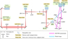 |
Fig. 17 Schematic representation of the CRAL XAO test bench, with two wavefront correctors a SLM and a DM followed by the iMZ with its two symmetrical and anti-symmetrical pupils re-imaged on a single camera ANDOR Neo. The iMZ coronagraphic output is re-imaged on a separate camera ANDOR Zyla. A tip-tilt corrector (PI-TT) is used for fine alignment on the iMZ pinhole. |
Experimental parameters used for closed-loop experiments with the iMZ.
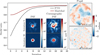 |
Fig. 18 Experimental laboratory results of closed-loop correction with the iMZ, a 12 × 12 DM, and for a full circular pupil. Left: evolution of the Strehl ratio for 20 iterations of the loop with a gain g = 0.3. The Strehl ratio measured with the optical transfer function (OTF) (dashed black line) is compared with the Maréchal approximation (solid purple line). The mismatch between the two curves comes from an underestimation of the phase (over estimation of the Strehl ratio) because some points of the input phase screen are higher than π/2 radians and the signal is wrapped. The four images under Strehl curves represent the PSFs (left) and the coronagraphic PSFs (right) for the first (up) and last iterations (down). Right: wavefronts measured by the iMZ (asymmetric output) for the first (up) and last iterations (down). |
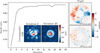 |
Fig. 19 Experimental laboratory results of closed-loop correction with the iMZ, a 12 × 12 DM, and for the ELT pupil. Left: evolution of the Strehl ratio (measured by the OTF) for 20 iterations of the loop with a gain g = 0.3 and coronagraphic PSFs (right) at first (up) and last iteration (down). Right: wavefront surface measured with the iMZ (asymmetric output) at first (up) and last iterations (down). |
7.3 Experimental validation of the iMZ performances on the complex ELT pupil
In the previous sections, we validated the performances of the iMZ for XAO on giant telescopes highlighting a preferred usage as a second stage XAO system to cope with bad turbulence conditions by reducing the level of phase aberrations in order to maximize its performances. Second stage XAO will be impacted by some imperfections linked to the first stage AO correction such as petal modes. In this last section, we present experimental iMZ measurements performed on ELT petal modes which are differential piston between the fragment of the pupil separated by the spider vanes and is responsible for a strong degradation in the imaging quality (Levraud et al. 2024). These modes can appear in closed-loop AO fragmented pupils telescopes (projection of the telescope spider vanes onto the pupil) due to the inability of phase-derivative-sensitive WFS (Shack–Hartmann, Pyramid) to measure this type of aberration in the presence of pupil discontinuities. The low wind effect phenomenon (Sauvage et al. 2015, Milli et al. 2018) as described in Sect. 7.1.1 also contributes to the appearance of these structures. The iMZ sensitivity to petal modes is here addressed experimentally in the ELT pupil configuration, with two different static phase screens applied to an SLM. The first one corresponds to fragment continuous pistons, where a random phase value between -π and π is applied to each fragments. The highest piston is set at –2.4 rad (240 nm), with a peak-to-valley over the pupil of 1.2 π rad (380 nm) and a phase variance of 2 rad2 (RMS = 140 nm). We present in Fig. 20 the phase correction of theses piston aberrations from petal modes with a 12 × 12 DM.
As one of the pistons’ values exceeds π/2 rad (open loop dynamic of the iMZ), a single measurement with the iMZ does not allow one to restore the full aberration dynamic (phase folded into the sine function, for a phase of |φ| > π/2, the sensor measures a phase equal to π - φ). In the hypothesis of perfect measurement and correction, a minimum of three iterations is therefore required to correct the –2.4 rad piston. The closed-loop measurements of Fig. 20 are presented with and without flux adjustment of the calibration parameters. The results obtained in both configurations after five iterations is similar, with 93–94% of Strehl obtained. We notice however that correction with flux adjustment of α̂c and β̂c converges faster, with 77% Strehl after two iterations compared with only 55% without flux adjustment. The structures visible on the residual maps on Fig. 20 are mainly caused by the DM fitting error, and are stronger at the transition between two pistons with the largest phase jumps. Nevertheless, the iMZ measurements quality is very good (Strehl greater than 93%) and the flux adjustment is only required at the initialization of the loop when the aberrations are high and can be optional if the phase errors remain within [-π, π].
Other static aberrations, at smaller spatial scales, are likely to degrade the ELT image quality, such as polishing residuals at the scale of the primary mirror segments. In Fig. 21, we present the experimental results of the iMZ phase measurement of a phase screen encoding these ELT static aberrations (used for HARMONI simulation, see Zieleniewski et al. 2015) and their correction by the SLM.
As is shown in Fig. 21, the initial phase map shows various differential piston residuals at the ELT fragment scale, as well as aberrations at the hexagonal segment scale (polishing residuals), ranging from −530 to 670 nm. The static aberration phase screen is projected onto the SLM’s 256 levels and measured with the iMZ, by applying the calibration with the SLM command applied (i.e the calibration phase diversity steps are produced on top of the phase to be measured). The upper part of Fig. 21 shows the SLM command (left), the iMZ measured phase (center) and the residual phase (right) measured by the iMZ after applying the measured correction to the SLM. We can see that most of the structures are correctly measured. The phase measurements are very precise at all spatial scales above 20 cm on the ELT pupil. The phase variance measured on the pupil is reduced from 0.59 rad2 to 0.12 rad2 . The effects of the correction is also visible in the image plane, with a much sharper PSF after correction, with an estimated Strehl ratio of 82% after correction versus 66% before correction. By imaging the pupil on a large number of pixels, ≈1000 here, we demonstrate that the iMZ can also measure precisely aberrations at very high spatial scales, here 6–10 times higher than the ELT segment size. For this experimental validation, the spatial resolution is not limited by the iMZ itself but is set by the restricted field of view on the bench.
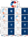 |
Fig. 20 Experimental demonstration of a five iterations correction with a 12 × 12 DM of differential pistons, generated with an SLM, for the ELT pupil and measured with the iMZ. A random value between -π and π is given to each of the six pistons, for a pupil variance of ≈2 rad2. For iteration 0, 2, 4 and 5 (rows) pupil image and associated PSF are displayed, with (left) and without (right) flux adjustment. The Strehl ratio is estimated with the maximum ADU of the image relative to the reference PSF. |
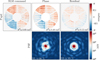 |
Fig. 21 Experimental demonstration of iMZ measurements efficiency of ELT static residuals (polishing, differential pistons...) (from HAR-MONI simulations, Zieleniewski et al. 2015) and correction with a 512 × 512 SLM. Upper left: SLM phase commands. Center upper part: phase measured with the iMZ, by calibrating directly on the statics SLM map and corresponding PSF (Center Low part). Right upper part: phase in the pupil plane measured with the iMZ, after the SLM correction has been applied and corresponding PSF (Right lower part). |
8 Conclusion
This work focuses on the iMZ and its use in XAO in various telescope contexts. Wavefront measurement, particularly at the speed required to correct for atmospheric turbulence, remains a major challenge in AO, especially for difficult observations such as direct imaging of exoplanets from a terrestrial telescope. Significant research resources are therefore currently being deployed around the world to meet this challenge, particularly in the context of the entry into operation, in the next decade, of a new generation of telescopes such as the ELT. We have presented new methods to push the limits of the iMZ WFS toward greater dynamical range and toward using it in a nonlinear regime. It required the development of an accurate model and the implementation of dedicated methods such as phase modulation, phase unwrapping, and calibration by adjusting the parameters of the sensor model by inverse approach. We evaluated the influence of measurement noise on the estimation of the iMZ model parameters, and therefore on the reconstructed phase, to validate its ultimate precision at the theoretical limit. The iMZ reconstruction errors taking into account noise propagation have been compared between analytical models and simulations, showing a very good agreement and providing orders of magnitude of the number of photons necessary to achieve accuracies compatible with the XAO needs. A comparative analysis of the iMZ WFS with other candidate WFSs for the XAO, such as the pyramid sensor (PyWFS) and the Zernike mask, has been presented in a common formalism. The proposed iMZ WFS demonstrates a high sensitivity, slightly lower than that of the unmodulated pyramid WFS. We found that for the 2 λ/D pinhole iMZ, the reduction of propagated photon noise standard deviation could reach a factor of 1.22, meaning that it needs  times more photons than the unmodulated PyWFS to reach a similar measurement precision. This comparison also highlights the gain in sensitivity of the Zernike sensor for small phases below half a wave, with ~2 times fewer photons needed to achieve the same measurement precision than the iMZ. The comparison with the Zernike is particularly relevant, since the Zernike WFS is one of the most sensitive WFSs used in AO. We showed that the iMZ dynamical range, reduced to a wave in closed loop, can be extended to several waves by using phase diversity strategies.
We have demonstrated, in simulations and experimentally, a new calibration method for the iMZ, which is an essential step for the precise reconstruction of the phase. It is achieved by inverse approach using the proposed interferometric model of the data. The level of modeling presented here made it possible to characterize the performances in the different operating modes of the iMZ depending on the system parameters (such as the size of the filtering pinhole). The E2E numerical simulation made it possible to simulate the iMZ WFS used in closed loop to measure its impact on improving images, and therefore on directly contributing to HCI. The E2E simulations made it possible to characterize the response of the iMZ as a function of the measured distortions (atmospheric turbulence) and different settings (with or without modulation, taking into account the flux variation with the input phase or not). We simulated the performance of the iMZ in a complete AO loop, for different pupil configurations, notably those of an 8-meter telescope, for which the iMZ is used as first or second correction stage, as well as for an ELT configuration. The first case studied corresponds to that of a high-contrast AO system on an eight-meter VLT-type telescope, and different regimes are considered. The results show that, with the right settings, the iMZ makes it possible to obtain excellent correction levels that are very competitive with the ones obtained with a pyramid WFS. Our E2E uses an iMZ without a first stage of correction provided that phase modulation and unwrapping are implemented and show very good performances. In low-flux cases (1 photon per pixel and per frame at the entrance of the sensor), the iMZ measurement makes it possible to achieve, in a good seeing regime, correction levels greater than 50% of Strehl. As a second stage WFS, we have shown using the COMPASS-based SAXO+ numerical simulator that the performances of iMZ are comparable to the ones expected with the pyramid sensor (87% Strehl obtained with 5 photons per pixel per frame). We highlight the necessity of tiptilt pre-correction for the iMZ, which can be easily managed by a servo loop using the PSF or coronagraphic outputs from the iMZ device. E2E simulations have also shown that it is possible to change the operating mode of the iMZ online, depending on the conditions, starting for example with a high dynamical range to close the OA loop, before moving to a mode favoring sensitivity, once the AO loop has stabilized. This versatility makes the iMZ particularly attractive. We also studied the effects of increasing the spectral band on the sensitivity of the iMZ, over a spectral band of 400 nm. We showed that there is a clear performance gain to widen the spectral band in closed-loop operations, which is similar to the photon-collected gain because the decrease in visibility when using polychromatic light remains small in this regime.
The development of the iMZ is also motivated by the arrival of ELTs leading to the new challenging optical aberrations, such as differential pistons between different segments constituting the pupil, and the “petal” modes that come from the fragmentation of the pupil of this type of telescope. The performance of the iMZ for this configuration has been analyzed in detail, and we have demonstrated that over a certain range of amplitudes the iMZ is sensitive to these modes, which represents a great advantage. The absolute phase measurement capacity of the iMZ is key, and the simulations demonstrate that even in the first stage (under favorable seeing and flux conditions) the iMZ could measure the entire wavefront phase errors, including turbulence and pupil fragmentation. We have also confirmed the high iMZ sensitivity to the LWE, using realistic phase screens to simulate the response of the ELT/METIS instrument AO system. The experimental implementation of the iMZ on the XAO laboratory bench at CRAL made it possible to measure deformations as small as a few nanometers. We have also demonstrated experimentally the phase unwrapping method of extending the iMZ dynamic by using a deformable mirror influence function and static turbulent phase screens. These results are particularly encouraging with respect to the use of iMZ in a regime of strong turbulence. The use of these methods in an real-time XAO loop to correct turbulent wavefront errors is the next step of this work. This experimental work demonstrates the good performances of the iMZ as part of a full AO loop, using a full pupil and a typical ELT pupil, even in the presence of differential piston aberrations.
The iMZ, by providing an absolute measurement of the phase and a dynamical range adapted to good observing conditions, appears to be a promising candidate for future ELT instruments such as PCS. With its two complementary outputs, the iMZ offers the possibility of measuring the amplitude of the incident wave jointly with its phase, and hence possibly of correcting the effects of atmospheric scintillation.
Acknowledgements
The authors are grateful to the LABEX Lyon Institute of Origins (ANR-10-LABX-0066) Lyon for its financial support within the Plan France 2030 of the French government operated by the National Research Agency (ANR). The authors are grateful to the PEPR Origins (WP1.1 – AO WFS – ANR-22-EXOR-0002) for its financial support within the Plan France 2030 of the French government operated by the National Research Agency (ANR). This work was also supported by the Action Spécifique Haute Résolution Angu-laire (ASHRA), PNP and PNPS of CNRS/INSU co-funded by CNES and by the CNRS Commission Spécialisée Astronomie-Astrophysique. We acknowledge funding from the Live-Mirror project funded from the European Union’s Horizon Europe research and innovation programme HORIZON-EIC-2022-PATHFINDEROPEN-01 under grant agreement No. 101099220. The authors are grateful to Markus Feldt for providing the low wind effect phase screen sequences developed for METIS and to Valentin Fonteneau for his help with the SLM calibration.
References
- Angel, J. R. P. 1994, Nature, 368, 203 [Google Scholar]
- Bertrou-Cantou, A., Gendron, E., Rousset, G., et al. 2022, A&A, 658, A49 [NASA ADS] [CrossRef] [EDP Sciences] [Google Scholar]
- Beuzit, J. L., Vigan, A., Mouillet, D., et al. 2019, A&A, 631, A155 [NASA ADS] [CrossRef] [EDP Sciences] [Google Scholar]
- Boccaletti, A., Chauvin, G., Mouillet, D., et al. 2020, arXiv e-prints [arXiv:2003.05714] [Google Scholar]
- Cantalloube, F., Dohlen, K., Milli, J., Brandner, W., & Vigan, A. 2019, The Messenger, 176, 25 [NASA ADS] [Google Scholar]
- Cerpa-Urra, N., Kasper, M., Kulcsár, C., Raynaud, H.-F., & Taïssir Heritier, C. 2022, J. Astron. Telesc. Instrum. Syst., 8, 019001 [NASA ADS] [CrossRef] [Google Scholar]
- Chambouleyron, V., Fauvarque, O., Plantet, C., et al. 2023, A&A, 670, A153 [NASA ADS] [CrossRef] [EDP Sciences] [Google Scholar]
- Dallant, J., Langlois, M., Flasseur, O., & Thiébaut, É. 2023, A&A, 679, A38 [NASA ADS] [CrossRef] [EDP Sciences] [Google Scholar]
- Degiorgio, V. 1980, Am. J. Phys., 48, 81 [Google Scholar]
- Delacroix, C., Langlois, M. P., Loupias, M., et al. 2015, SPIE Conf. Ser., 9617, 96170G [Google Scholar]
- Dohlen, K., Decortiat, F., Fresneau, F., & Lanzoni, P. 1998, SPIE Conf. Ser., 3352, 551 [Google Scholar]
- Dohlen, K., Langlois, M., Lanzoni, P., et al. 2006, SPIE Conf. Ser., 6267, 626734 [Google Scholar]
- Fang, C., Huang, J.-Z., Li, H., Li, Y., & Zeng, G. 2019, Appl. Phys. Lett., 115, 031101 [Google Scholar]
- Feldt, M., Bertram, T., Correia, C., et al. 2024, Exp. Astron., 58, 20 [Google Scholar]
- Ferreira, F., Gratadour, D., Sevin, A., et al. 2018, SPIE Conf. Ser., 10703, 1070347 [NASA ADS] [Google Scholar]
- Flasseur, O., Denis, L., Thiébaut, É., & Langlois, M. 2020, A&A, 637, A9 [NASA ADS] [CrossRef] [EDP Sciences] [Google Scholar]
- Fusco, T., Sauvage, J. F., Petit, C., et al. 2014, SPIE Conf. Ser., 9148, 91481U [NASA ADS] [Google Scholar]
- Galland, N., Raynaud, H. F., Kasper, M., et al. 2023, in Adaptive Optics for Extremely Large Telescopes (AO4ELT7), 74 [Google Scholar]
- Ghiglia, D. C., & Romero, L. A. 1994, J. Opt. Soc. Am. A, 11, 107 [NASA ADS] [CrossRef] [Google Scholar]
- Goulas, C., Galicher, R., Vidal, F., et al. 2024, SPIE Conf. Ser., 13097, 1309769 [Google Scholar]
- Greivenkamp, J. E. 1984, Opt. Eng., 23, 350 [Google Scholar]
- Guyon, O. 2005, ApJ, 629, 592 [NASA ADS] [CrossRef] [Google Scholar]
- Haffert, S. Y. 2024, A&A, 683, A113 [NASA ADS] [CrossRef] [EDP Sciences] [Google Scholar]
- Haffert, S., Males, J., & Guyon, O. 2023, in Adaptive Optics for Extremely Large Telescopes (AO4ELT7), 79 [Google Scholar]
- Janin-Potiron, P., N’Diaye, M., Martinez, P., et al. 2017, A&A, 603, A23 [NASA ADS] [CrossRef] [EDP Sciences] [Google Scholar]
- Jovanovic, N., Martinache, F., Guyon, O., et al. 2015, PASP, 127, 890 [NASA ADS] [CrossRef] [Google Scholar]
- Kasper, M., Cerpa Urra, N., Pathak, P., et al. 2021, The Messenger, 182, 38 [Google Scholar]
- Keppler, M., Benisty, M., Müller, A., et al. 2018, A&A, 617, A44 [NASA ADS] [CrossRef] [EDP Sciences] [Google Scholar]
- Lagrange, A. M., Bonnefoy, M., Chauvin, G., et al. 2010, Science, 329, 57 [Google Scholar]
- Langlois, M., Loupias, M., Graf, C., & Moretto, G. 2023, Mach–Zehnder interferometric device, french Patent FR2301972 [Google Scholar]
- Levraud, N., Chambouleyron, V., Sauvage, J. F., et al. 2024, A&A, 682, A84 [NASA ADS] [CrossRef] [EDP Sciences] [Google Scholar]
- Loupias, M., Langlois, M., Thiébaut, E., Tallon, M., & Leger, J. 2016, SPIE Conf. Ser., 9909, 99094F [Google Scholar]
- Mach, L. 1892, Zeitsch. Instrument., 12, 89 [Google Scholar]
- Macintosh, B., Graham, J. R., Barman, T., et al. 2015, Science, 350, 64 [Google Scholar]
- Macintosh, B., Chilcote, J. K., Bailey, V. P., et al. 2018, SPIE Conf. Ser., 10703, 107030K [Google Scholar]
- Males, J. R., Close, L. M., Miller, K., et al. 2018, SPIE Conf. Ser., 10703, 1070309 [NASA ADS] [Google Scholar]
- Marois, C., Lafrenière, D., Doyon, R., Macintosh, B., & Nadeau, D. 2006, ApJ, 641, 556 [Google Scholar]
- Martins, D., Holzlöhner, R., Verinaud, C., & Kleinclaus, C. 2022, SPIE Conf. Ser., 12187, 1218712 [Google Scholar]
- Mawet, D., Bond, C. Z., Delorme, J. R., et al. 2018, SPIE Conf. Ser., 10703, 1070306 [NASA ADS] [Google Scholar]
- Mawet, D., Pueyo, L., Lawson, P., et al. 2012, SPIE Conf. Ser., 8442, 844204 [NASA ADS] [Google Scholar]
- Milli, J., Kasper, M., Bourget, P., et al. 2018, SPIE Conf. Ser., 10703, 107032A [Google Scholar]
- Nousiainen, J., Engler, B., Kasper, M., et al. 2024, J. Astron. Telesc. Instrum. Syst., 10, 019001 [NASA ADS] [Google Scholar]
- Plantet, C., Meimon, S., Conan, J. M., & Fusco, T. 2015, Opt. Express, 23, 28619 [NASA ADS] [CrossRef] [Google Scholar]
- Por, E. H., Haffert, S. Y., Radhakrishnan, V. M., et al. 2018, Proc. SPIE, 10703, 1070342 [Google Scholar]
- Ragazzoni, R. 1996, J. Mod. Opt., 43, 289 [Google Scholar]
- Rousset, G., Primot, J., & Fontanella, J. C. 1987, LEST Foundation, Technical Report, 28, 17 [Google Scholar]
- Sauvage, J.-F., Fusco, T., Guesalaga, A., et al. 2015, in Adaptive Optics for Extremely Large Telescopes IV (AO4ELT4), E9 [Google Scholar]
- Schreiber, L., Langlois, M., Jolissaint, L., et al. 2023, in Adaptive Optics for Extremely Large Telescopes (AO4ELT7), 126 [Google Scholar]
- Schwartz, N., Sauvage, J.-F., Correia, C., et al. 2018, SPIE Conf. Ser., 10703, 1070322 [NASA ADS] [Google Scholar]
- Scott, D. W. 1992, Multivariate Density Estimation: Theory, Practice, and Visualization (John Wiley & Sons, Inc.) [Google Scholar]
- Thiébaut, E., & Tallon, M. 2010, J. Opt. Soc. Am. A, 27, 1046 [Google Scholar]
- Vigan, A., Dohlen, K., Surdej, I., Yaitskova, N., & Gonte, F. 2010, SPIE Conf. Ser., 7733, 773353 [Google Scholar]
- Zehnder, L. 1891, Zeitsch. Instrum., 11, 275 [Google Scholar]
- Zernike, F. 1934, Mon. Not. Roy. Astron. Soc., 94, 377 [Google Scholar]
- Zieleniewski, S., Thatte, N., Kendrew, S., et al. 2015, MNRAS, 453, 3754 [Google Scholar]
Hence, the pixelwise parameters, denoted in boldface in previous equations, are replaced by the scalar parameters, denoted with normal characters, for the pixel of interest.
Which holds for a small phase aberration ϕ and a small phase modulation w.
The most demanding operation of the unwrapping process is the Discrete Cosine Transform (DCT) with computation time of the order of N log2 N with N the number of pixels in the pupil and using Fast Fourier Transform (FFT) to compute the DCT. Using a straightforward version of the algorithm written in Julia we measured 400 microseconds to unwrap a 200 × 200 phase screen on a simple laptop with a single Intel Core i7-13800H CPU.
All Tables
Photonic phase measurement error (standard deviation in nanometers) calculated analytically.
Photonic phase measurement error (in nanometers) calculated from the simulated residual standard deviation.
Simulation parameters used for closed-loop simulation for a single-stage XAO using the iMZ.
All Figures
|
Fig. 1 Schematic representation of the iMZ WFS. (a) The iMZ component. (b) Light path from the pupil plane preceding the iMZ to the detector. (c) Lateral view of the pinhole side of the iMZ, with ρ1 the amplitude reflection coefficient on Side 1 (see later Table 1). |
| In the text | |
|
Fig. 2 Experimental demonstration of high dynamics phase measurement with the iMZ: reconstruction of the influence function of one of the 140 actuators of the CRAL XAO test bench MEMS deformable mirror (see Sect. 7.2.2 for more details about the experimental setup). Upper panel: pupil plane images of the (a) raw intensity measured on the asymmetric iMZ output, (b) phase retrieved by the arcsine without modulation, (c) phase retrieved by the two-argument arc-tangent with modulation and (d) phase obtained by unwrapping the phase in (c). All phases have been extracted given the calibrated model parameters (see Sect. 5.1). Bottom panel: horizontaL cut of the actuator influence function centered at its peak for the different retrieved phases. at different stages of reconstruction. |
| In the text | |
|
Fig. 3 Variances of the iMZ phase estimators (in rad2, logarithmic scale) as a function of N the number of photons per pixel per frame available for measurement for the λ/D pinhole diameter and 40/60 beam splitter. The expressions of the estimators are given in Eqs. (12) and (14). The solid lines plot the theoretical variances, given in Eqs. (30) and (31), for the joint (in blue), symmetric (in green), and asymmetric (in orange) MLEs of the phase. The dashed lines correspond to the simulated results for a null input phase. |
| In the text | |
|
Fig. 4 Analytical photon noise variance (in rad2, logarithmic scale) as functions of the number, N, of photons per pixel per frame available for the phase measurement at the entrance of various WFSs: the SHWFS (in orange, Rousset et al. 1987), the unmodulated PYWFS (in green, Chambouleyron et al. 2023), the 1.06 λ/D and 2λ/D dot diameter ZWFS (in blue, Chambouleyron et al. 2023, Haffert et al. 2023) and the iMZ in purple for a λ/D (solid line) and 2λ/D (dashed line) diameter pinhole. |
| In the text | |
|
Fig. 5 Noise-free simulation of iMZ response for a monochromatic (1000 nm) and broadband (800–1200 nm uniformly cut into 11 intervals 40 nm wide) light source, for an input aberration of 250 nm RMS (top left). The flux is 10 photons/pixel for each spectral interval (hence 11 times more photons in total for the broadband source compared to the monochromatic one). The interferograms’ intensities are displayed as a percentage of the incident flux. Top left: random incident wavefront phase produced by the DM actuators. Top right: interferograms obtained for each iMZ output (symmetrical in blue, asymmetrical in orange), monochromatic (solid line) and polychromatic (dotted line). Bottom: vertical section through the pupil diameter of the four interferograms. The visibility was calculated as V = (Imax - Imin)/(Imax + Imin), with Imin and Imax the minimal and maximal intensities measured in the image of the pupil. |
| In the text | |
|
Fig. 6 Simulation of the iMZ phase measurements for a monochromatic (left) and polychromatic (right) light source, for the 50 nm RMS incident aberration (wavefront from Fig. 5 divided by 5). |
| In the text | |
|
Fig. 7 Experimental result of iMZ signal calibration using the asymmetric output, with three different phase offsets applied to the DM in addition to the phase diversity steps required to perform the calibration. First row: peak-to-valley ≈140 nm, σ2 ≈ 0.06 rad2. Second row: peak-to-valley ≈ 250 nm, σ2 ≈ 0.1 rad2. Third row: peak-to-valley ≈310 nm, σ2 ≈ 0.5 rad2. The first line correspond to raw focal plan images produced behind the pinhole with the three DM settings. The second line shows the pupil plane signal of the asymmetric output. Lines 3 to 5 show the measured calibration parameters N αa, Nβ, and ϕ estimated with weighted least mean square method for these three DM settings. The DM shape is shown for comparison on the last line. |
| In the text | |
|
Fig. 8 Variations in the model parameters with the filtered relative amplitude, γ. (a) The parameters αs, αa, and β (in percent of the incident flux) as functions of γ, see Eqs. (77a)-(77c). (b) Radial cut of γ for a flat wavefront and pinhole diameters from 0.5 to 4 λ/D. (c) Mean value of γ in the pupil for a phase aberration with taking values from -π/2 to π/2 and whose shape is one of the fifty first Zernike modes, for a λ/D pinhole. Below the curve we show the PSFs in logarithmic scale for Z1, Z2, Z4, and Z25. The pinhole diameter is overlaid with a black circle. The percentages indicated for each Zernike mode corresponds to the PSF energy encircled within the pinhole. |
| In the text | |
|
Fig. 9 Closed-loop results with the iMZ on 1 second of turbulence, for 0.4 arcsecond seeing, with tip-tilt pre-correction. Upper panel: evolution of the residual phase variance (rad2) during 1000 iterations of correction at 1 kHz for different flux conditions (magnitude 5 ≤ m ≤ 14). Lower panel: residual phase variance (rad2) and Strehl ratio (averaged over the last 500 iterations) as a function of the number N of inward pho-tons/pixel/frame. The blue crosses indicates the photon noise limit of the iMZ (1.5/N) according to the theoretical variance in Sect. 3. |
| In the text | |
|
Fig. 10 Single-stage closed-loop results obtained with the iMZ using 1 second of evolving turbulence, for 0.4 arcsecond seeing, with tip-tilt pre-correction. Asymmetric iMZ output intensity (first row), measures phase command (second row), residual phase maps (third row) and short exposure PSF (fourth row) for a magnitude 7 guide star (N = 108 photons/pixel/frame). The piston has been removed from both phase commands and phase residual maps. |
| In the text | |
|
Fig. 11 Closed-loop result with the iMZ on 1 second of turbulence, for 0.7 arcsecond seeing, with tip-tilt pre-correction. Upper panel: residual phase variance (rad2) evolution over 1000 iterations of correction at 1 kHz for different flux conditions (m ∈ [5...13], without (solid line) and with modulation + unwrapping (dashed line). Lower panel: associated Strehl ratio estimated at 1.2 µm. |
| In the text | |
|
Fig. 12 Closed-loop results with the iMZ on 1 second of turbulence, for 0.7 arcsecond seeing, with tip-tilt pre-correction, without (upper) and with phase modulation (lower). Residual phase error (1st row) and short exposure PSF (2th row) for a magnitude 8 (N = 43 photons/pixel/frame). The piston has been filtered out from the residual maps. |
| In the text | |
|
Fig. 13 Schematic representation of a second stage with an iMZ WFS, in cascade with the current SAXO AO system, to simulate SAXO+. The first stage is simulated by COMPASS, to generate realistic first-stage residuals. |
| In the text | |
|
Fig. 14 Median seeing SAXO+ simulation with the iMZ as a second stage WFS. The upper graph shows the evolution of phase residual variance (in logarithmic scale) over 1000 correction iterations (loop frequency = 1 kHz) for N = 3 photons/pixel/frame (blue curve). The evolution of phase residual variance after SAXO is overplotted in black (loop frequency = 150 Hz for N = 5 photons/pixel/frame). The lower pictures show residual phase maps and short-exposure focal plane images (log scale) at the beginning and at the end of the one second sequence. |
| In the text | |
|
Fig. 15 E2E simulation of the iMZ response in closed-loop using a 500 ms sequence (quasi-static) of LWE for the ELT pupil. The upper graph shows the evolution of the phase variance (rad2 ) with time and the associated Strehl ratio during the 500 iterations of AO closed-loop correction with iMZ wavefront sensing. Lower images show the iMZ phase maps at the beginning and at the end of the sequence and the corresponding PSFs. |
| In the text | |
|
Fig. 16 Simulation of the iMZ response with the ELT pupil in closed-loop to ten different atmospheric turbulence sequences corresponding to very good seeing (0.4 arcseconds) and flux conditions (m = 5). Upper part: evolution of the residual phase variance for one second of turbulence, generated with HCIPy (Por et al. 2018). Each of the ten curves correspond to a different turbulence sequence with r0 = 15 cm (42 cm at 1.2 µm) and L0 = 25 m. Bottom part: residual phase maps and corresponding PSFs at the last iteration for three of the ten sequences, representing three typical cases. |
| In the text | |
|
Fig. 17 Schematic representation of the CRAL XAO test bench, with two wavefront correctors a SLM and a DM followed by the iMZ with its two symmetrical and anti-symmetrical pupils re-imaged on a single camera ANDOR Neo. The iMZ coronagraphic output is re-imaged on a separate camera ANDOR Zyla. A tip-tilt corrector (PI-TT) is used for fine alignment on the iMZ pinhole. |
| In the text | |
|
Fig. 18 Experimental laboratory results of closed-loop correction with the iMZ, a 12 × 12 DM, and for a full circular pupil. Left: evolution of the Strehl ratio for 20 iterations of the loop with a gain g = 0.3. The Strehl ratio measured with the optical transfer function (OTF) (dashed black line) is compared with the Maréchal approximation (solid purple line). The mismatch between the two curves comes from an underestimation of the phase (over estimation of the Strehl ratio) because some points of the input phase screen are higher than π/2 radians and the signal is wrapped. The four images under Strehl curves represent the PSFs (left) and the coronagraphic PSFs (right) for the first (up) and last iterations (down). Right: wavefronts measured by the iMZ (asymmetric output) for the first (up) and last iterations (down). |
| In the text | |
|
Fig. 19 Experimental laboratory results of closed-loop correction with the iMZ, a 12 × 12 DM, and for the ELT pupil. Left: evolution of the Strehl ratio (measured by the OTF) for 20 iterations of the loop with a gain g = 0.3 and coronagraphic PSFs (right) at first (up) and last iteration (down). Right: wavefront surface measured with the iMZ (asymmetric output) at first (up) and last iterations (down). |
| In the text | |
|
Fig. 20 Experimental demonstration of a five iterations correction with a 12 × 12 DM of differential pistons, generated with an SLM, for the ELT pupil and measured with the iMZ. A random value between -π and π is given to each of the six pistons, for a pupil variance of ≈2 rad2. For iteration 0, 2, 4 and 5 (rows) pupil image and associated PSF are displayed, with (left) and without (right) flux adjustment. The Strehl ratio is estimated with the maximum ADU of the image relative to the reference PSF. |
| In the text | |
|
Fig. 21 Experimental demonstration of iMZ measurements efficiency of ELT static residuals (polishing, differential pistons...) (from HAR-MONI simulations, Zieleniewski et al. 2015) and correction with a 512 × 512 SLM. Upper left: SLM phase commands. Center upper part: phase measured with the iMZ, by calibrating directly on the statics SLM map and corresponding PSF (Center Low part). Right upper part: phase in the pupil plane measured with the iMZ, after the SLM correction has been applied and corresponding PSF (Right lower part). |
| In the text | |
Current usage metrics show cumulative count of Article Views (full-text article views including HTML views, PDF and ePub downloads, according to the available data) and Abstracts Views on Vision4Press platform.
Data correspond to usage on the plateform after 2015. The current usage metrics is available 48-96 hours after online publication and is updated daily on week days.
Initial download of the metrics may take a while.