| Issue |
A&A
Volume 701, September 2025
|
|
|---|---|---|
| Article Number | A156 | |
| Number of page(s) | 12 | |
| Section | Planets, planetary systems, and small bodies | |
| DOI | https://doi.org/10.1051/0004-6361/202555533 | |
| Published online | 15 September 2025 | |
Gas and dust dynamics in γ Cephei-type disks
1
Department of Physics and Astronomy, University of Padova,
via Marzolo 8,
35131
Padova,
Italy
2
Theoretical Division, Los Alamos National Laboratory,
Los Alamos,
NM
87545,
USA
★ Corresponding authors: This email address is being protected from spambots. You need JavaScript enabled to view it.
; This email address is being protected from spambots. You need JavaScript enabled to view it.
Received:
15
May
2025
Accepted:
7
August
2025
Abstract
Context. Giant planets are observed orbiting the primary stars of close binary systems. Such planets may have formed in compact circumprimary disks, which once surrounded these stars, under conditions much different than those encountered around single stars.
Aims. In order to quantify the effects of the strong gravitational perturbations exerted on circumprimary disk material, the three-dimensional (3D) dynamics of gas and dust in orbit around the primary star of a compact and eccentric binary system was modeled by applying the stellar and orbital parameters of γ Cephei, a well-known system that can be representative of a class of close binaries.
Methods. Circumprimary gas was approximated as an Eulerian viscous and compressible fluid and modeled by means of 3D hydrodynamical simulations, assuming locally isothermal conditions in the medium around the primary star. Dust grains were modeled as Lagrangean particles, subjected to gravity and aerodynamic drag forces. Models that include a giant planet were also considered.
Results. Models indicate that spiral density waves excited around pericenter passage propagate toward the inner boundary of the disk, through at least a few pressure scale-heights from the mid-plane, inducing radial and vertical mixing in the gas. However, perturbations imparted to gas, both in terms of eccentricity and precession, are far weaker than previously estimated by two-dimensional (2D) simulations. Models predict small eccentricities, ≲0.03, and slow retrograde precession. The addition of a giant planet does not change the low eccentricity state of the disk. The parameters applied to the disk would lead to the formation of a massive planet, many times the mass of Jupiter, in agreement with some observations. Micron to mm-size dust grains are well coupled to the gas, resulting in similar dynamics and statistically similar distributions of orbital elements. The planet only affects the dust distributions locally. In agreement with outcomes of recent 2D models, the lifetime of an isolated circumprimary disk would be brief, ~105 years, because of its compact nature, requiring a long-term external supply of mass to allow for the in situ formation of a giant planet.
Key words: planets and satellites: formation / planets and satellites: gaseous planets / planets and satellites: general / protoplanetary disks / planet-disk interactions / binaries: close
© The Authors 2025
 Open Access article, published by EDP Sciences, under the terms of the Creative Commons Attribution License (https://creativecommons.org/licenses/by/4.0), which permits unrestricted use, distribution, and reproduction in any medium, provided the original work is properly cited.
This article is published in open access under the Subscribe to Open model. This email address is being protected from spambots. You need JavaScript enabled to view it. to support open access publication.
1 Introduction
γ Cephei is a 3 Gyr-old, close-binary system located approximately 14 parsecs away (Baines et al. 2018). The presence of a low-mass stellar companion, γ Cephei B, was first reported by Campbell et al. (1988) and first imaged by Neuhäuser et al. (2007). The primary star, γ Cephei A, hosts a substellar-mass companion within ≈2 au (Hatzes et al. 2003). If this object formed around the primary star, it did so in a highly perturbed environment, considering that it orbits at around 1/6 of the binary’s pericenter distance. Importantly, γ Cephei is not peculiar in this regard, as planetary-mass companions observed in compact and eccentric binaries are not rare. Indeed, γ Cephei can be considered as a representative of a class of binary systems.
In fact, according to the catalog of exoplanets in binary systems1 maintained by Schwarz et al. (2016), there are at least 20 systems, with separations between 10 and ≈50 au, which host a planet more massive than 0.1 Jupiter masses (MJ). Surprisingly, 60% of these binaries are eccentric, with orbital eccentricities in the range from ≈0.1 to ≈0.5. Since tidal interactions between orbiting material and the stars are expected to truncate the circumprimary disk at ≈25% of the binary’s semi-major axis, these systems would be surrounded by compact disks extending from a few to ≈12 au from the primary. Therefore, in these systems, planet formation occurs (if it does) in a very small disk.
An initial assessment on the conditions required to form a massive planet around γ Cephei A indicated the need for a relatively large gas density in the circumprimary disk (Thébault et al. 2004), a condition required by the small disk size. Such an outcome may be aided by tidal confinement driven by the orbital eccentricity of the binary. However, in these situations, additional complications may affect formation by core accretion. A short list includes: (a) the circumprimary disk lifetime, which must exceed ~106 years to allow for the growth of a giant planet; (b) the availability and supply of solid material, which must be sufficient to form the initial core of the planet; (c) solid dynamics, which must be conducive to accumulation, rather than fragmentation, an outcome affected by the highly perturbed gas dynamics. This paper looks into the details of the circumprimary disk evolution to provide constraints on both gas and dust dynamics. We do so by performing three-dimensional (3D) simulations of the evolution of the gas and dust in a disk orbiting the primary of a γ Cephei-type system. We consider disk configurations both before and after the possible formation of a giant planet. In particular, we focus on disk eccentricity, which appears to be significantly smaller than that estimated by previous two-dimensional (2D) simulations. In addition, the precession rate of the disk is much slower and both these results may have profound implications on the evolution of planetesimals in the disk (Beaugé et al. 2010; Silsbee & Rafikov 2015). Mass transport through the disk, and toward the primary star, is enhanced by a factor of a few compared to the expectations of unperturbed, steady-state disks around single stars, as a result of its compact nature and inward propagation of spiral waves excited around pericenter passage.
When a massive planet is included in the circumprimary disk, a deep gap forms around the planet’s orbit and dust grains accumulate outside the gap. We calculate the migration rate of the planet and estimate its mass accretion rate. Under the assumption of sustained supply of gas, from an external source, the planet may easily reach a mass several to many times the mass of Jupiter. This prediction is in agreement with some observational estimates (Benedict et al. 2018).
It was suggested by previous work on compact binaries (Picogna & Marzari 2013) that hydraulic jumps at the locations of spiral density waves might excite the distribution of the dust orbital inclination, possibly slowing down the process of sedimentation toward the disk mid-plane and therefore hindering or preventing streaming instability from forming planetesimals. In these calculations, we consider a number of particles large enough, and with different sizes, to test the effects of the perturbations caused by spiral waves on the orbital evolution of dust.
The results of the models presented herein can be used to characterize gas and dust dynamics around the primaries of binary systems with masses comparable to γ Cephei A and B, and with similar orbital separations and eccentricities. Applicability of these models is obviously constrained by the physical description of the system adopted in the simulations. The applied methods are described in Section 2 and the physical specifications are given in Section 3. The results of the calculations are discussed in Sections 4 and 5. We present our conclusions in Section 6.
2 Numerical methods
The gas surrounding the primary star was approximated to a viscous and compressible fluid, through the Navier-Stokes equations, which were solved in three dimensions by means of a finite-difference algorithm, second-order accurate in space and time (see D’Angelo & Bodenheimer 2013, and references therein). Two dimensional versions of the 3D models were also simulated to highlight major differences. In order to mitigate restrictions on the calculation time-step, imposed by the Courant–Friedrichs–Lewy condition, orbital advection (Masset 2000) was applied as described in D’Angelo & Marzari (2012).
The 3D disk domain was rendered and discretized in spherical coordinates {r, θ, ϕ}, with origin on the primary star ({r, ϕ} coordinates were used in 2D; note that we use the same notation for the polar radius in 3D and the cylindrical radius in 2D). The domain extends 2π in azimuth (ϕ) around the primary and is symmetric with respect to the mid-plane (θ = π/2). The gravity field is given through the potential
![Mathematical equation: $\[\Phi=\Phi_{\mathrm{A}}+\Phi_{\mathrm{B}}+\Phi_p+\Phi_{\mathrm{I}},\]$](/articles/aa/full_html/2025/09/aa55533-25/aa55533-25-eq1.png) (1)
(1)
where ΦA and ΦB are the potentials of the primary and secondary star, respectively, and Φp is the potential generated by planet (when applicable). The last term on the right-hand side is the indirect potential arising from non-inertial forces generated by the motion of the origin of the reference frame,
![Mathematical equation: $\[\Phi_{\mathrm{I}}=\frac{G M_{\mathrm{B}}}{r_{\mathrm{B}}^3} \mathbf{r} \cdot \mathbf{r}_{\mathrm{B}}+\frac{G M_p}{r_p^3} \mathbf{r} \cdot \mathbf{r}_p.\]$](/articles/aa/full_html/2025/09/aa55533-25/aa55533-25-eq2.png) (2)
(2)
The planet potential, Φp, was smoothed over a length RH/5, where RH is the planet’s Hill radius (no softening is applied to the stellar potentials). Gas self-gravity was neglected. Note that, although the choice of the reference frame is arbitrary, a reference system with origin on the primary is best suited to describe the dynamics of circumprimary disk. In simulations that include the planetary body, the orbits were integrated by means of a variable order and adaptive step-size Gragg-Bulirsch-Stoer extrapolation algorithm (Hairer et al. 1993), requiring convergence at machine precision.
We used two grids with 1142 × 22 × 630 and 1902 × 22 × 1048 grid elements, respectively. Some models including a giant planet were also computed on a 1142 × 22 × 1260 grid. Models in two dimensions have the same grid structures in the radial and azimuthal directions. Outflow boundary conditions were applied at the outer radial boundary and reflective boundary conditions were applied at the inner radial boundary and at the disk surface. After models achieve equilibrium states, outflow boundary conditions are also applied at the radial inner boundary so that gas can flow toward the primary. Boundary conditions applied herein do not allow for possible delivery of material to the circumprimary disk from a circumbinary disk (not modeled in these calculations). At the level of gas viscosity and pressure scale-height applied in the models, the tidal barrier maintained by the stars is strong enough that the supply of both gas and dust to the circumprimary disk would be negligible during the simulated timescales. In fact, Marzari & D’Angelo (2025, hereafter, MD25) showed that a circumbinary disk with comparable gas parameters would supply gas to the circumprimary disk at a rate ~10−8 M⊙ yr−1, adding a trivial amount of mass during the simulations.
Solids were modeled as Lagrangian (collision-less) particles, interacting through gravity with the stars and through drag with the gas. Particle thermodynamics was computed and evolved as described in D’Angelo & Podolak (2015). The initial distribution of silicate dust comprises 20 000 particles, distributed in equal numbers into four size bins of radius Rs = 1 μm, 10 μm, 100 μm, and 1 mm. Since gas temperatures around the primary may significantly exceed ice evaporation temperatures (see, e.g., Picogna & Marzari 2013; Jordan et al. 2021), we modeled silicate grains with a material density ϱs = 2.648 g cm−3. Solids that move past the radial and vertical boundaries become inactive. Solids that cross the disk mid-plane are reflected, mimicking dust motion across the mid-plane.
3 Physical and numerical parameters
Stellar and orbital parameters representative of γ Cephei are used to represent a class of binary systems. Therefore, since we intend the models to be broadly applicable to close and eccentric binaries, the precise values of these parameters are not important. In fact, there are still inconsistencies in the stellar masses reported in the literature. Here we choose the values derived by Neuhäuser et al. (2007), MA = 1.4 M⊙ (see also Baines et al. 2018) and MB = 0.4 M⊙. These values are close to those derived more recently by Mugrauer et al. (2022), MA = 1.3 M⊙ and MB = 0.38 M⊙. Neuhäuser et al. values provide a secondary to primary mass ratio of q = 0.286, quite close to the mass ratio resulting from the estimates of Mugrauer et al. (2022), q = 0.292. We note that Torres (2007) estimated somewhat lower masses, MA = 1.2 M⊙ and MB = 0.36 M⊙, which nonetheless result in a similar mass ratio, q = 0.3. The binary separation is set to a = 20 au and its orbital eccentricity to e = 0.4 (Endl et al. 2011; Mugrauer et al. 2022). With these parameters, the binary period is T = 66.667 years.
The primary star, γ Cephei A, has a substellar-mass companion whose minimum mass was estimated at 1.85 Jupiter masses (Endl et al. 2011). The actual mass of this object may in fact be much larger. Analysis of astrometry measurements acquired by the Hubble Space Telescope resulted in a value of 9.4 Jupiter masses (Benedict et al. 2018). The model planet, however, has to be smaller than its final mass since it is still surrounded by gas and, thus, would be actively accreting (e.g., Bodenheimer et al. 2013). Lacking firm constraints, we use the parameters derived by Endl et al. (2011): Mp = 1.85 MJ, ap = 2.05 au and ep = 0.049. The planet’s orbit is coplanar with the binary orbit, and both lie in the disk mid-plane.
The primary disk is initialized with a gas surface density Σ ∝ 1/r, where r indicates the distance from the primary in both 2D and 3D geometry, and a relative pressure scale-height H/r = 0.05. Models apply a local-isothermal equation of state
![Mathematical equation: $\[P=c_s^2 \rho,\]$](/articles/aa/full_html/2025/09/aa55533-25/aa55533-25-eq3.png) (3)
(3)
where ρ is the gas density and cs the local-isothermal sound speed (the gas temperature around the primary is ∝ 1/r). Because of Eq. (3) and the neglect of disk self-gravity, gas dynamics can be re-scaled by the initial density. We use au as units of length and MA/au2 as units of surface density. Viscous stresses in the gas are implemented through a time-constant kinematic viscosity ν = αH2ΩK, where ΩK is the local Keplerian frequency around the primary and α = 0.001. No artificial viscosity (e.g., Stone & Norman 1992) is used in these calculations. A summary of some of the main parameters adopted in the models is reported in Table 1.
According to theoretical expectations based on a comparison between tidal torques and viscous stresses at Lindblad resonances, for the stellar and disk parameters applied herein (MB/MA, e, α, and H/r), tidal truncation of the circumprimary disk is expected between the inner 1:9 and 1:8 commensurability of the binary, around r/a ≈ 0.23–0.25 (Artymowicz & Lubow 1994). Since these models are intended to describe only the circumprimary disk and considering the above requirement on tidal truncation, the disk domain extends from r = 0.005 a to 0.575 a (0.1–11.5 au) around the primary, within the pericenter of the secondary. In 3D, the disk extends about 3.5 pressure scale-heights above the mid-plane.
System parameters.
4 Gas dynamics
This section presents results on the dynamics of the gas in the circumprimary disk, separately introducing models without a giant planet and models that include a giant planet. Except for the different gravitational potential, Eqs. (1) and (2), these models use the same physical and numerical parameters. Models including a planet were only simulated in three dimensions.
4.1 Circumprimary disk without a giant planet
The circumprimary disk of close and eccentric binaries, is expected to be very small. The truncation radius occurs in the proximity of the inner 1:8 mean-motion resonance of the binary, ≈5 au from the primary in the case of γ Cephei. Nonetheless, outward viscous diffusion (see Lynden-Bell & Pringle 1974; Pringle 1981) would be inhibited or largely prevented by the tidal field of the stars, preserving a significant reservoir of material into a compact disk. For the initial conditions applied herein, the circumprimary disk mass is ≈0.01 MA. This material would be depleted via accretion onto the primary star and possibly replenished via accretion from a circumbinary disk (MD25). The disk lifetime would be determined by these two competing processes (photo-evaporation and surface winds may also contribute).
Figure 1 illustrates the gas density ρ in the r-θ plane (top panels) and the surface density Σ (middle panels), after ≈600 binary periods (T), when the disk has achieved a quasi-equilibrium state (see discussion below). The color scale is logarithmic; ρ is in units of MA/au3 and Σ is in units of MA/au2. The three images on each row refer to different phases of the binary orbit: apocenter passage (left), pericenter passage (center), and soon after pericenter passage (right), when the disk is perturbed the most. The binary orbit is fixed in the models that do not include a giant planet, because the gravity of disk material is neglected, and the setup is such that the secondary transits apocenter at time t = n T, for any integer n. As a reference, when the secondary is at apocenter, the orbital phase is π (the star lies on the negative X axis in the left panels of Figure 1). In the figure (right), the orbital phase is ≈π/3, which occurs ≈0.06 T after pericenter passage (center panels). Since the deformation of the disk depends on the phase of the binary, the gas density in a vertical slice depends on the azimuth around the primary at which it is selected. In the top panels of the figure, the azimuth angle of the slice is ≈0.3π in all three cases. Therefore, in the top-right panel, the slice is nearly aligned with and in the same direction as the secondary star.
The bottom panels of Figure 1 show the surface density resulting from a corresponding 2D model, at the same times as in the middle panels. The tidal deformation of the 2 D disk is significantly larger than that of the 3D disk, as can be visually estimated by comparing the density contours in the middle and bottom images. This outcome stems from the fact that, in the 2D geometry, all disk material is confined to the orbital plane of the binary, where the tidal field is the strongest.
Tidal deformation and density wave propagation would also modify the local temperature of the gas in the affected regions. These variations are not modeled here because of the applied local-isothermal equation of state. However, when averaged over the binary period (or longer times), temperature asymmetries around the primary tend to cancel out (see, e.g., Picogna & Marzari 2013).
Density waves excited around pericenter passage propagate inward, from the edge of the circumprimary disk, inducing perturbations that affect the entire vertical column of the disk, as shown in Figure 2. The traveling waves stir the vertical motion of the gas, ahead and behind of the wave fronts, as indicated by the projected streamlines over-plotted to the density distribution. The images represent phases soon after pericenter passage (top and middle) and soon prior apocenter passage. The behavior of the streamlines suggests the occurrence of large-scale mixing throughout the disk. Vertical stirring of the gas and eddies with a vertical extent ≳H continue after pericenter passage. It is expected that this mixing motion be reflected in the motion of dust grains that are well coupled to the gas. As a result, vigorous radial and vertical mixing of small dust grains may ensue.
The gas surface density averaged around the primary is reported in Figure 3, for the 2D and 3D models of Figure 1, as indicated. The thicker curves represent the mean profiles over a binary period whereas the shaded regions provide the range of variation during that period. The tidal truncation radius is not well defined and, for a given binary mass ratio and eccentricity, depends on gas pressure and turbulence viscosity. Referring to the figure, this radius may be defined as the location where ⟨Σ⟩ changes slope and declines more rapidly. Under this definition, truncation occurs between ≈0.2 a (3D model) and ≈0.25 a (2D model). Despite the fact that the two models in Figure 3 are in very different states, quasi-circular one and eccentric the other (as discussed below), these predictions agree with the theoretical estimates of Artymowicz & Lubow (1994). The 2D models presented in MD25 have a shorter truncation radius than the 2D model in the figure, consistent with the fact that they applied a smaller pressure scale-height in the circumprimary disk (see also Artymowicz & Lubow 1994).
The 3D model of Figures 1 and 3 predicts that a negligible amount of gas is lost through the outer boundary and, therefore, the circumprimary disk only depletes through accretion on the primary (and through other possible removal processes at the surface). Viscosity-driven transport in a steady-state accretion disk, 3π⟨Σν⟩ (Lynden-Bell & Pringle 1974), would result in an accretion rate toward the star (averaged throughout the disk) of ≈10−7 M⊙ yr−1. This analytical approximation does not, however, account for the angular momentum transferred by the secondary during close encounters. In fact, the density waves, excited around pericenter passage, travel inward, depositing angular momentum in the disk material. Since density waves propagate inward of r/a = 0.1 (see Figure 2), angular momentum deposition is expected to affect the mass transport throughout the disk and accretion onto the primary. Following MD25, we employ tracer particles to obtain fluid trajectories and determine a time-averaged mass transport in the disk. Passive tracers are deployed in 60 radial bins, from the inner boundary out to r = 6 au. Each radial bin initially contains 600 particles, distributed over 2π in azimuth (around the primary) and over 3 H above the mid-plane. Particle trajectories are integrated for a time 2 T and their average radial displacement during this period is used to quantify the average radial velocity of the fluid, ⟨ur⟩. The mass flux F = ρ⟨ur⟩ (here ρ is the density at the initial location of a tracer) is aggregated over all tracers, in each of the initial radial bins, to obtain a time-averaged accretion rate ![Mathematical equation: $\[\langle\dot{m}\rangle\]$](/articles/aa/full_html/2025/09/aa55533-25/aa55533-25-eq4.png) as a function of r. Results indicate that
as a function of r. Results indicate that ![Mathematical equation: $\[\langle\dot{m}\rangle\]$](/articles/aa/full_html/2025/09/aa55533-25/aa55533-25-eq5.png) fluctuates in the region most affected by density waves, confirming that their perturbing effects persist over the entire binary period. In the more quiescent inner region r ≤ 1 au (r/a ≤ 0.05),
fluctuates in the region most affected by density waves, confirming that their perturbing effects persist over the entire binary period. In the more quiescent inner region r ≤ 1 au (r/a ≤ 0.05), ![Mathematical equation: $\[\langle\dot{m}\rangle\]$](/articles/aa/full_html/2025/09/aa55533-25/aa55533-25-eq6.png) has a mean value of ≈ −2.5 × 10⁻⁷ M⊙ yr−1, approximately twice as large as the analytical estimate provided above for steady-state disks (around single stars). An additional estimate of
has a mean value of ≈ −2.5 × 10⁻⁷ M⊙ yr−1, approximately twice as large as the analytical estimate provided above for steady-state disks (around single stars). An additional estimate of ![Mathematical equation: $\[\langle\dot{m}\rangle\]$](/articles/aa/full_html/2025/09/aa55533-25/aa55533-25-eq7.png) was derived by monitoring the time variations of the circumprimary disk mass, as gas flows across the inner radial boundary. The value, ≈ −3 × 10⁻⁷ M⊙ yr−1, is consistent with the estimate provided by the analysis of tracers.
was derived by monitoring the time variations of the circumprimary disk mass, as gas flows across the inner radial boundary. The value, ≈ −3 × 10⁻⁷ M⊙ yr−1, is consistent with the estimate provided by the analysis of tracers.
This large value of ![Mathematical equation: $\[\langle\dot{m}\rangle\]$](/articles/aa/full_html/2025/09/aa55533-25/aa55533-25-eq8.png) would result in a rapid removal of gas from around the primary, over a timescale of ~105 years (see also MD25). Notice that, although the accretion rate depends on the choice of the initial density, the removal timescale only depends on viscosity, pressure scale-height and binary parameters. Clearly, giant planet formation via core accretion would be unfeasible over such brief timescales. A steady supply of material from a circumbinary disk would be required for such a mechanism to operate. A much smaller (by factors of tens) turbulence viscosity could extend the lifetime of the disk. However, it would not alleviate the problem of the limited reservoir of solids orbiting the primary, which may hinder the assembly of a large enough planetary core required to form a giant planet. In fact, this latter requirement would argue in favor of the concurrent presence of a circumbinary disk and of some non-trivial turbulence level in the gaseous medium.
would result in a rapid removal of gas from around the primary, over a timescale of ~105 years (see also MD25). Notice that, although the accretion rate depends on the choice of the initial density, the removal timescale only depends on viscosity, pressure scale-height and binary parameters. Clearly, giant planet formation via core accretion would be unfeasible over such brief timescales. A steady supply of material from a circumbinary disk would be required for such a mechanism to operate. A much smaller (by factors of tens) turbulence viscosity could extend the lifetime of the disk. However, it would not alleviate the problem of the limited reservoir of solids orbiting the primary, which may hinder the assembly of a large enough planetary core required to form a giant planet. In fact, this latter requirement would argue in favor of the concurrent presence of a circumbinary disk and of some non-trivial turbulence level in the gaseous medium.
The early phases of planet formation would be aided by the largely circular motion of the disk gas attained in the 3D models, which would tend to reduce relative velocities among solids and promote growth. Predictions of 2D models would instead further complicate planetary assembly. In fact, previous 2D models indicated that, starting from a circular and unperturbed state, the circumprimary disk settles into a quasi-equilibrium, eccentric state after 400–500 T (Jordan et al. 2021). A local disk eccentricity, ed, is often defined by projecting the motion of fluid elements on two-body orbits around the star. This quantity is then mass-weighted over the disk domain to obtain a bulk disk eccentricity
![Mathematical equation: $\[\left\langle e_d\right\rangle=\frac{\int e_d \mathrm{~d} m}{\int \mathrm{~d} m},\]$](/articles/aa/full_html/2025/09/aa55533-25/aa55533-25-eq9.png) (4)
(4)
in which the mass element is dm = Σrdrdϕ. If the mass average is performed only over the angular coordinates, ⟨ed(r)⟩ provides the mass-weighted disk eccentricity at a given radius. In a 3D disk, the motion of a fluid element is projected on a two-body orbit in the disk mid-plane. The results of this approximation are validated in Section 5.1, by using the trajectories of fine dust.
Figure 4 illustrates the evolution of the mass-weighted disk eccentricity, for 2D and 3D models. Consistently with prior studies, the 2D disk settles into an eccentric state that reaches equilibrium after several hundred binary periods. There is a large difference between the predictions of the 2D and 3D model, with the former projecting a quasi-equilibrium eccentric state at ⟨ed⟩ ≈ 0.3 (green circles) and the latter resulting in a quasi-circular circumprimary disk, ⟨ed⟩ ≈ 0.03 (orange circles). Moreover, the 3D model attains quasi-equilibrium much sooner, after ≈100 T. The lines in Figure 4 represent averages over 10 T. A comparison at the grid resolutions used herein (see Section 2) indicates that 2D results are insensitive whereas 3D results at higher resolution predict a lower mass-weighted eccentricity, ⟨ed⟩ ≈ 0.025. A linear regression to model data during the last ≈100 T indicates that ⟨ed⟩ is practically constant.
As mentioned above, the quantity ⟨ed(r)⟩ measures the local eccentric deformation of the disk. In the 2D model, ⟨ed(r)⟩ rapidly increases outward, reaching above ≈0.3 at r = 1 au and ≈0.5 at r = 3 au. In the 3D model, ⟨ed(r)⟩ remains ≲0.03 inside 4 au, and only starts to increase around the truncation radius. Results presented in Section 5, on the orbital eccentricity of fine dust, can also be used to gauge the local eccentricity of the gas.
Picogna & Marzari (2013) performed radiative SPH calculations of close binary disks and found eccentricities around the primary between 0.02 and 0.06 (see also Martin et al. 2020). These results are comparable to those of Figure 4. There are, however, important differences between their approach and ours. They considered a larger mass ratio, q = 0.4, and a wider orbit, a = 30 au. They modeled the gas thermodynamics and obtained a different aspect ratio of the circumprimary disk. Moreover, viscous stresses in the gas are not directly comparable between SPH and Eulerian hydrodynamics.
A definition similar to the mass-weighted disk eccentricity in Eq. (4) can be introduced for the mass-weighted argument of pericenter of the disk
![Mathematical equation: $\[\left\langle\omega_d\right\rangle=\frac{\int \omega_d \mathrm{~d} m}{\int \mathrm{~d} m}.\]$](/articles/aa/full_html/2025/09/aa55533-25/aa55533-25-eq10.png) (5)
(5)
The evolution of the argument of pericenter of the circumprimary disk is presented in Figure 5 for 2D (top panel, green circles) and 3D (orange circles) models. In the top panel, the time axis starts at some reference time, around the end of the simulations, when the models have already achieved equilibrium states. In 2D, the disk shows retrograde precession at a rate ![Mathematical equation: $\[\left\langle\dot{\omega}_{d}\right\rangle \approx -\Omega / 6\]$](/articles/aa/full_html/2025/09/aa55533-25/aa55533-25-eq11.png) , where Ω = 2π/T is the binary orbital frequency (see also Jordan et al. 2021). The disk precession rate is determined by a balance between gravitational and pressure forces, in which the former provide a prograde contribution to precession whereas the latter provide a retrograde contribution (e.g.,Lubow 1992; Goodchild & Ogilvie 2006). The 2D standard model of Jordan et al. (2021) has physical parameters comparable to those of the 2D calculation in Figure 5, although the numerical setups differ. They also found retrograde precession, but at a lower (i.e., less negative) rate. The difference could be related to their somewhat cooler disk (smaller H/r), which favors prograde precession. Their results also suggest that the 2D precession rate scales as (H/r)2, and that it transitions from retrograde to prograde for H/r ≲ 0.02 (for the setup they implemented, see their Fig. 17).
, where Ω = 2π/T is the binary orbital frequency (see also Jordan et al. 2021). The disk precession rate is determined by a balance between gravitational and pressure forces, in which the former provide a prograde contribution to precession whereas the latter provide a retrograde contribution (e.g.,Lubow 1992; Goodchild & Ogilvie 2006). The 2D standard model of Jordan et al. (2021) has physical parameters comparable to those of the 2D calculation in Figure 5, although the numerical setups differ. They also found retrograde precession, but at a lower (i.e., less negative) rate. The difference could be related to their somewhat cooler disk (smaller H/r), which favors prograde precession. Their results also suggest that the 2D precession rate scales as (H/r)2, and that it transitions from retrograde to prograde for H/r ≲ 0.02 (for the setup they implemented, see their Fig. 17).
Figure 5 also shows that, in the 3D model, the precession rate of the circumprimary disk is much slower (top panel, orange circles) than the 2D estimate. The bottom panel of the figure displays the long term evolution of the argument of pericenter in the 3D model. The solid line provides an average every 10 T. A linear regression for times t > 400 T indicates that precession is still retrograde, but at a rate ![Mathematical equation: $\[\left\langle\dot{\omega}_{d}\right\rangle \approx-5 \times 10^{-5} \Omega\]$](/articles/aa/full_html/2025/09/aa55533-25/aa55533-25-eq12.png) . Therefore, the choice of model parameters (MA/MB, H/r, and ν) produces a near balance between gravity and pressure effects. To investigate how close to prograde precession this configuration is, the 3D model of Figure 5 was continued for an additional period of ≈250 T, by setting a smaller pressure scale-height. To remove possible effects due to changes in kinematic viscosity, ν, the turbulence parameter α was adjusted so to preserve the product αH2. The results of these additional models suggest that the transition from a retrograde to prograde circumprimary disk is very close and occurs between H/r ≈ 0.045 and 0.04.
. Therefore, the choice of model parameters (MA/MB, H/r, and ν) produces a near balance between gravity and pressure effects. To investigate how close to prograde precession this configuration is, the 3D model of Figure 5 was continued for an additional period of ≈250 T, by setting a smaller pressure scale-height. To remove possible effects due to changes in kinematic viscosity, ν, the turbulence parameter α was adjusted so to preserve the product αH2. The results of these additional models suggest that the transition from a retrograde to prograde circumprimary disk is very close and occurs between H/r ≈ 0.045 and 0.04.
An eccentric gaseous disk with a significant precession rate, like the one resulting from the 2D model discussed here, was also found by Kley & Nelson (2008) under similar initial conditions. Gas dynamics in such disks is expected to have important consequences on the dynamics of planetesimals (Beaugé et al. 2010; Silsbee & Rafikov 2015). In a binary configuration such as the one we consider herein, Beaugé et al. (2010) showed that, on average, the relative impact velocities between planetesimals increase with respect to the case of a circular, non-precessing disk. These more energetic impacts are particularly relevant for small, kilometre-size planetesimals, and may prevent their growth into larger bodies. Pair-wise impacts involving larger planetesimals, or involving two bodies with a large size difference, can still lead to accretion but mainly in the outer regions of the disk (see Fig. 7 of Beaugé et al. 2010). In addition, planetesimals undergo an enhanced orbital decay in semi-major axis due to gas drag caused by the increase in relative velocities. These effects would stave off, hinder or delay the formation of a planetary core massive enough to grow into a giant planet. However, the scenario predicted by our 3D simulations suggests that the disk eccentricity is relatively small and the precession rate (either retrograde or prograde) is very slow (under our assumptions). Both occurrences would promote a more efficient planetesimal accumulation in the circumprimary disk of close binary systems. Other physical effects have been shown to be effective in reducing the disk eccentricity even in 2D models, such as self-gravity (Marzari et al. 2009) and a better treatment of the gas thermodynamics (Marzari et al. 2012; Müller & Kley 2012), both of which are expected to be relevant in massive young disks. Jordan et al. (2021) presented 2D simulations in which they found ed ≈ 0.2 and suggested that the low disk eccentricity found in radiative disks by Marzari et al. (2012) and Müller & Kley (2012) may have been a consequence of low numerical resolution and high gas viscosity. Our findings, from the 3D simulations, indicate that a low disk eccentricity and slow precession may be common outcomes at most stages of the circumprimary disk evolution.
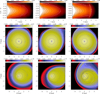 |
Fig. 1 Top panels: volume gas density in a vertical slice (r-θ), in units of MA/au3 and logarithmic scale, obtained from a 3D model. The distributions are displayed at a phase of the binary orbit around apocenter passage (left), pericenter passage (center), and shortly thereafter (right). Middle and bottom panels: surface density of the gas, in units of MA/au2 and logarithmic scale, at the same orbital phases as in the top panels, obtained from the 3D model (middle) and from a corresponding 2D model (bottom). |
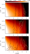 |
Fig. 2 Volume gas density in a r-θ plane, in units of MA/au3 and logarithmic scale, from the 3D model of Figure 1. The orbital phase of the binary corresponds to a time ≈0.06 T (top) and ≈0.13 T (middle), after pericenter passage, and ≈0.1 T prior to apocenter passage (bottom). The curves with arrows are streamlines of the gas velocity projected in the r-θ plane (different streamline colors are used to enhance the contrast against the density color-map). The waves excited by the secondary propagate inward, stirring the vertical and radial motion of the gas. |
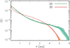 |
Fig. 3 Surface density averaged around the primary, in units of MA/au2, obtained from the 3D (red) and 2D (green) models of Figure 1. The thicker curves represent the mean profile computed over an orbital period of the binary, T. The shaded regions indicate maximum and minimum density values attained during the orbit. |
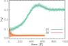 |
Fig. 4 Mass-weighted disk eccentricity, Eq. (4), of the circumprimary disk versus time. The 2D model predicts an eccentric disk, achieving quasi-equilibrium at ⟨ed⟩ ≈ 0.3 (green circles). The solid line is an average performed every 10 T. In comparison, the 3D model predicts a much less eccentric circumprimary disk (orange circles), ⟨ed⟩ ≈ 0.03. The red curve represents an average over 10 T intervals. |
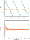 |
Fig. 5 Mass-weighted argument of pericenter of the circumprimary disk versus time. The top panel shows results for a 2D (green circles) and a 3D model (orange circles). The 2D model predicts a retrograde precession of the circumprimary disk at a rate of about 6 binary periods for a full revolution. The precession rate resulting from the 3D model is still retrograde, but orders of magnitude slower. The long-term behavior of the 3D model is displayed in the bottom panel. The solid line represent an average over 10 T intervals. See text for further details. |
4.2 Circumprimary disk with a giant planet
In contrast to the models presented in Section 4.1, in models that include a giant planet orbiting the primary, the binary orbit varies because of stars-planet gravitational interactions. One consequence is that there is prograde precession of the argument of pericenter of the binary orbit, at an average rate of ≈2 × 10⁻⁵ Ω, where Ω is the initial orbital frequency of the binary. The same gravitational interactions also affect the planet’s orbit, which displays a retrograde precession of its argument of pericenter at an average rate of ≈−10−3 Ω.
Maps of the gas density in the disk with the embedded planet are illustrated in Figure 6. Similarly to top and middle panels of Figure 1, the mass density (in units of MA/au3 and logarithm scale) in r-θ planes is shown in the top panels, in which each plane contains the planet, at different phases of the binary orbit: apocenter passage (left), pericenter passage (center), and soon after pericenter passage (right). The bottom panels render the surface density (in units of MA/au2 and logarithmic scale) at the same orbital phases of the binary. Comparing the top panels of Figures 6 and 1, it is possible to assess the added perturbations arising from the density waves launched by the planet to those arising from the waves launched by the secondary star. Stirring of disk material induced by the planet’s gravity adds to that induced by the secondary (see Figure 2) and, therefore, an increased amount of mixing in the gaseous medium should ensue. In principle, this enhanced mixing could be reflected in the vertical distribution of fine dust since settling could be altered. However, as we will discuss in Section 5, in terms of global features stirring added by the planet does not significantly impact the vertical distribution of dust.
The mean eccentricity of the disk, according to Eq. (4), has an average value ⟨ed⟩ ≈ 0.03, the same as in the configuration without the planet. However, ⟨ed⟩ has a somewhat larger variability during the binary period, from ≈0.025 to ≈0.04. By separating the contributions arising from the gas interior and exterior to the planet orbit, ⟨ed⟩ ranges between ≈0.015 and ≈0.02 inside the orbit and between ≈0.03 and ≈0.05 outside.
The implication is that the added planet potential is not affecting much the eccentric perturbation on the gas, which is basically dominated by the gravity field of the binary. However, there can be local effects, mostly confined to the proximity of the planet’s orbit. In Section 5, we also use the orbital eccentricity of fine dust as proxy to track the local gas eccentricity.
As indicated in Figure 6, the planet’s potential produces a deep gap in the disk, which is also shown in the azimuthally-averaged profiles of surface density in Figure 7. A condition for gap formation (D’Angelo & Lubow 2010),
![Mathematical equation: $\[\left(\frac{M_p}{M_{\mathrm{A}}}\right)^2>3 \pi f \alpha\left(\frac{H}{a_p}\right)^5,\]$](/articles/aa/full_html/2025/09/aa55533-25/aa55533-25-eq13.png) (6)
(6)
is largely fulfilled by the model setup (the factor f depends on the distribution of torques exerted by the planet on the disk). Note that the planet-to-primary mass ratio only marginally exceeds the Jupiter-to-Sun mass ratio. The depth of the gap agrees well with expectations from analytic theory and calculations of disk-planet tidal interactions. For example, the formulations of Kanagawa et al. (2015) and Duffell (2015) predict a density within the gap of ≈2 × 10⁻⁶, in the units of Figure 7.
Compared to the mean density profile of the disk without a planet (shaded region, see Figure 3), the disk is denser outside of the gap region, as a result of material displaced from around the planet’s orbit. In fact, the gap forms because the tidal field of the planet supplies angular momentum to material exterior to the orbit and removes it from material interior to the orbit. Nonetheless, as in the models of Section 4.1, the mass flux through the outer open boundary is negligible, and the circumprimary disk only depletes through accretion on the primary and the planet (not considering possible removal processes at the surface).
Three-body problem dynamics places a stability limit of ≈3.8 au to the planet distance from the primary (Holman & Wiegert 1999). However, interactions with the disk material can affect this limit, and orbital dynamics in general. In fact, variations of the planet’s orbital elements, due to the gravity field of the stars alone, occur on extremely long timescales, ~108 T for ap whereas ep executes oscillations in the range 0.044–0.064 over ≈90 T. Experiments conducted by allowing the planet’s orbit to change under torques exerted by the disk gas indicate that the orbit tends to shrink and circularize. Orbital migration occurs at an average rate ![Mathematical equation: $\[\left\langle\dot{a}_{p}\right\rangle \approx-0.01 ~\mathrm{au} / T\]$](/articles/aa/full_html/2025/09/aa55533-25/aa55533-25-eq14.png) whereas orbital eccentricity damps at a rate
whereas orbital eccentricity damps at a rate ![Mathematical equation: $\[\left\langle\dot{e}_{p}\right\rangle \sim-0.0001 / T\]$](/articles/aa/full_html/2025/09/aa55533-25/aa55533-25-eq15.png) (undergoing oscillations over several binary periods). These experiments neglect tidal torques exerted by the dust on the planet, since the models include a limited number of individual particles.
(undergoing oscillations over several binary periods). These experiments neglect tidal torques exerted by the dust on the planet, since the models include a limited number of individual particles.
A rapid evolution of the orbital elements of the planet is expected since the circumprimary disk extends only for about 2.5 times the orbital radius of the planet and is ten times as massive. In particular, the migration timescale is short but still within the canonical Type II regime expected of gap-opening planets (see, e.g., Baruteau et al. 2014, and references therein). In fact, D’Angelo & Lubow (2010) showed that orbital migration of gap-opening planets can be described analogously to Type I migration (of non-gap-opening planets), through a torque density distribution that peaks at ≈RH on either side of r = ap and is non-zero within ≈3 RH of the orbit. Therefore, migration can be described as Type I, but driven by the average density within 2–3 RH of the planet’s orbit (see also Kanagawa et al. 2018). In Figure 7, this average density is about two orders of magnitude lower than the unperturbed density (black curve). Clearly, the model configuration would allow for inward migration of the planet on a relatively short timescale so that the orbital parameters in Table 1 would not be final values (i.e., after gas disperses).
The model configuration would also allow for continued growth of the planet. Estimates of the accretion rate, at the viscosity level adopted in the model and ⟨Σ⟩ in Figure 7, indicate a value of a few times 10−5 MJ yr−1 (Lissauer et al. 2009; Bodenheimer et al. 2013). But this rate would rapidly decline as Mp increases. A simple estimate of the planet mass based on these rates would result in a final value of ≈9 MJ, assuming a constant density ⟨Σ⟩ a few times as low as in Figure 7 to account for depletion. Incidentally, some observations suggest that the planet is actually very massive, over 9 MJ (Benedict et al. 2018). Regardless, our model setup would be conducive to a massive giant planet, provided an external source of gas.
Mass growth would also alleviate the migration issue since the depth of the gap region reduces as Mp increases. The Type I migration speed is proportional to the planet mass, but the average density driving migration (inside 2–3 RH of the planet’s orbit) is ![Mathematical equation: $\[{\propto} M_{p}^{-2}\]$](/articles/aa/full_html/2025/09/aa55533-25/aa55533-25-eq16.png) (e.g., Kanagawa et al. 2015; Duffell 2015), so that the migration rate reduces with planet mass (e.g., Ida et al. 2018). However, both growth and migration of a planetary body orbiting the primary require considerations about the lifetime of the gaseous disk. As discussed in Section 4.1, an isolated disk would be removed on a short, ~105 yr timescale. A circumbinary disk would need to be in place to supply material and prolong the disk lifetime. Over the long term (i.e., the lifetime of the circumbinary disk), such a supply rate would also determine the surface density in the circumprimary disk in which the planet evolves. According to the estimates of MD25, the circumbinary supply rates,
(e.g., Kanagawa et al. 2015; Duffell 2015), so that the migration rate reduces with planet mass (e.g., Ida et al. 2018). However, both growth and migration of a planetary body orbiting the primary require considerations about the lifetime of the gaseous disk. As discussed in Section 4.1, an isolated disk would be removed on a short, ~105 yr timescale. A circumbinary disk would need to be in place to supply material and prolong the disk lifetime. Over the long term (i.e., the lifetime of the circumbinary disk), such a supply rate would also determine the surface density in the circumprimary disk in which the planet evolves. According to the estimates of MD25, the circumbinary supply rates, ![Mathematical equation: $\[\dot{M}_{\text {cb}}\]$](/articles/aa/full_html/2025/09/aa55533-25/aa55533-25-eq17.png) , could be of order 10−8 M⊙ yr−1, which would imply values of
, could be of order 10−8 M⊙ yr−1, which would imply values of ![Mathematical equation: $\[\langle\Sigma\rangle \sim \dot{M}_{\mathrm{cb}} /(3 \pi \nu)\]$](/articles/aa/full_html/2025/09/aa55533-25/aa55533-25-eq18.png) several times as low as in Figure 7. Applying a more detailed time integration of the planet mass using functions
several times as low as in Figure 7. Applying a more detailed time integration of the planet mass using functions ![Mathematical equation: $\[\dot{M}_{p}=\dot{M}_{p}\left(M_{p}\right)\]$](/articles/aa/full_html/2025/09/aa55533-25/aa55533-25-eq19.png) reported in Bodenheimer et al. (2013, see the Appendix therein) and density values determined by a declining supply rate
reported in Bodenheimer et al. (2013, see the Appendix therein) and density values determined by a declining supply rate ![Mathematical equation: $\[\dot{M}_{\mathrm{cb}}\]$](/articles/aa/full_html/2025/09/aa55533-25/aa55533-25-eq20.png) , of initial value ~10−8 M⊙ yr−1, the final mass of the planet could reach up to ≈8 MJ, as indicated by the evolution tracks reported in Figure 8.
, of initial value ~10−8 M⊙ yr−1, the final mass of the planet could reach up to ≈8 MJ, as indicated by the evolution tracks reported in Figure 8.
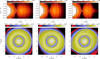 |
Fig. 6 Top panels: volume gas density in vertical slices, in units of MA/au3 and logarithmic scale, obtained from a 3D model that includes a giant planet. Each slice passes through the planet location. The distributions are displayed at a binary phase around apocenter passage (left), pericenter passage (center), and shortly thereafter (right). Bottom panels: surface density of the gas, in units of MA/au2 and logarithmic scale, plotted at the same orbital phases as in the top panels. |
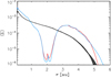 |
Fig. 7 Surface density averaged around the primary, in units of MA/au2, obtained from the 3D model of Figure 6. The density profiles correspond to orbital phases of the binary at apocenter (red) and pericenter (blue). The shaded region represents the surface density of the 3D model without a planet shown in Figure 3. The density peaks inside the tidal gap generated by the planet indicate the radial position of the planet (which moves on an eccentric orbit). |
 |
Fig. 8 Integration of the planet mass according to the accretion rates reported in Lissauer et al. (2009) and Bodenheimer et al. (2013), assuming that the circumprimary disk is supplied by the circumbinary disk with an initial accretion rate dMcb/dt as indicated, in units of M⊙ yr−1 (see MD25). The supply rate declines to zero over the circumbinary disk lifetime, a few million years in this example. See text for further details. |
5 Dust dynamics
Silicate grains are released in the circumprimary disk after it has evolved for about 330 T, when gas has achieved a quasi-equilibrium state (see Section 4). The evolution of the solids is modeled for ten binary periods thereafter. We model four size bins with radii Rs = 1 μm, 10 μm, 100 μm, and 1 mm. The initial distribution extends, radially, from the inner boundary of the computational domain out to r = 4.5 au and, vertically, over three pressure scale-heights H from the mid-plane.
5.1 Models without a giant planet
The distributions of the grains’ orbital semi-major axis (as), eccentricity (es), and inclination (is) are reported in Figure 9, when the secondary star is around apocenter (top) and pericenter passage (bottom). The histograms are stacked in order of increasing grain size, as indicated in the legends. The differences at the two binary phases are marginal, indicating that the dust orbital properties do not experience major variations during a binary period. In particular, semi-major axes and inclinations are quite similar. Some differences appear in the tails of the eccentricity distributions, which extend to higher values around pericenter passage. Statistically, however, the distributions are not distinguishable (see also Figure 10), as discussed further below. Around apocenter, ⟨es⟩ ≈ 0.04 with a cut-off at es ≈ 0.07 for all grain sizes. Around pericenter, the average eccentricity has a somewhat broader peak, ranging from es ≈ 0.02 to 0.06, at all dust sizes. These average values of eccentricity are consistent with those estimated for the eccentricity of gas elements in the disk.
The fact that the distributions of orbital properties do not display significant differences as a function of grain radius is mostly due to their small stopping time, τs (Whipple 1973; Weidenschilling 1977). Indicating with |u| the relative velocity between gas and a dust grain, the ratio of |u| to the drag acceleration defines the timescale over which gas and dust velocities converge. In the Epstein regime of free-molecular flow and |u| ≪ cs (e.g., Liffman & Toscano 2000; D’Angelo & Podolak 2015)
![Mathematical equation: $\[\tau_s \Omega_{\mathrm{K}} \approx\left(\frac{\varrho_s}{\rho}\right)\left(\frac{R_s}{H}\right).\]$](/articles/aa/full_html/2025/09/aa55533-25/aa55533-25-eq21.png) (7)
(7)
Recall that cs = HΩK (the thermal velocity of the gas is approximated to cs). The non-dimensional quantity τsΩK is referred to as Stokes number, St. For the applied parameters, within ≈ H of the disk mid-plane, St ≲ 10−6 for μm-grains and ≲ 10−3 for mm-grains. Since ρH ∝ Σ, St increases with r (see Figure 3). Dust dynamics is therefore well coupled to gas dynamics. Thus, the values of the dust eccentricity quoted above are expected to be consistent with the estimates of the gas eccentricity, provided in Section 4.1, for all dust sizes. Even if the long-term values of ⟨Σ⟩ were determined by the supply of gas from a circumbinary disk, as discussed in Section 4.2, and gas density was a factor of ~10 smaller, Stokes numbers would only be 10 times larger. The implication is that mm-grains would still be well coupled to the gas, and they would remain so until ⟨Σ⟩ declined below ~10 g cm−2, presumably toward the end of the circumbinary disk life.
When St ≪ 1, grains drift inward on a timescale (e.g., Takeuchi & Lin 2002; Chiang & Youdin 2010)
![Mathematical equation: $\[\tau_{\mathrm{drift}} \Omega_{\mathrm{K}} \sim \frac{1}{\mathrm{St}}\left(\frac{a_s}{H}\right)^2,\]$](/articles/aa/full_html/2025/09/aa55533-25/aa55533-25-eq22.png) (8)
(8)
whereas settling toward the mid-plane occurs on a typically much shorter timescale (e.g., Dullemond & Dominik 2004),
![Mathematical equation: $\[\tau_{\mathrm{sett}} \Omega_{\mathrm{K}} \sim \frac{1}{\mathrm{St}}.\]$](/articles/aa/full_html/2025/09/aa55533-25/aa55533-25-eq23.png) (9)
(9)
Note that both Eqs. (8) and (9) neglect effects of the orbital eccentricity and inclination of the grains. The drift timescale is long enough that even mm-grains should not move inward significantly during the modeled evolution of the disk (≈790 orbital periods at 1 au). This outcome is consistent with the histograms of Figure 9, left panels. The settling timescale is short enough for some settling to occur. Indeed, the right panels of Figure 9 indicate rapid dust sedimentation above ≈2H of the disk mid-plane, where ρ is very low and St is much larger than it is closer to the mid-plane. The distributions of the inclination, is, also show that there is an enhanced concentration of particles around the mid-plane (see histogram peaks at ![Mathematical equation: $\[i_{s}^{\circ}<0.5\]$](/articles/aa/full_html/2025/09/aa55533-25/aa55533-25-eq24.png) ), where the number density is larger than the initial value by a factor of several. These peaks appear at all particle sizes and have similar enhancements in number density (relative to the initial values). We performed a pair-wise comparison of the distributions of the particles’ inclination (see right panels of Figure 9), for all sizes. Results indicate that they are all similar, in that the difference in expected values (means) is compatible with zero (i.e., it is within the standard deviations of the distributions). This outcome is likely aided by vertical mixing induced by gas stirring (as shown in Figure 2).
), where the number density is larger than the initial value by a factor of several. These peaks appear at all particle sizes and have similar enhancements in number density (relative to the initial values). We performed a pair-wise comparison of the distributions of the particles’ inclination (see right panels of Figure 9), for all sizes. Results indicate that they are all similar, in that the difference in expected values (means) is compatible with zero (i.e., it is within the standard deviations of the distributions). This outcome is likely aided by vertical mixing induced by gas stirring (as shown in Figure 2).
Since the smallest, 1 μm grains are those that most closely follow gas dynamics, they can be used as a proxy to track gas orbital eccentricity. Figure 10 illustrates the eccentricity of the smallest dust, binned over 0.1 au intervals, as average value (dots) and standard deviation about the mean (error bars). The red symbols refer to dust orbiting within one scale-height H from the mid-plane, whereas the blue symbols refer to grains orbiting above H. Inside r ≈ 3 au (r/a ≈ 0.15), the fine particles located closer to the mid-plane have orbits somewhat more eccentric than those of particles located farther away. At larger distances from the star, differences subside as orbital eccentricity increases in the low density region of the circumprimary disk.
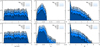 |
Fig. 9 Histograms of dust orbital properties obtained from a 3D model without a giant planet. Semi-major axis (left), eccentricity (center), inclination (right) of the solids are displayed at a binary phase around apocenter passage (top) and pericenter passage (bottom). Histograms are stacked in order of increasing dust size, as indicated in the legends. |
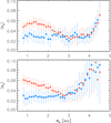 |
Fig. 10 Average orbital eccentricity of 1 μm-size dust, as function of semi-major axis, corresponding to the orbital phases of the binary of apocenter (top) and pericenter passage (bottom). Red symbols refer to grains within one scale-height H of the disk mid-plane whereas blue symbols refer to grains moving above H. Error bars provide the spread (standard deviation) of the distributions around the mean values. |
5.2 Models with a giant planet
The distributions of the dust semi-major axis, eccentricity, and inclination, for a 3D model containing a giant planet, are plotted in Figure 11, when the secondary is around apocenter (top) and pericenter passage (bottom). The peak around as ≈ 2–2.1 au is caused by particles orbiting the planet (see Table 1). Since the initial distribution of dust is uniform across the gap, these grains are leftovers of that local (initial) population, most of which is displaced from the gap region. In fact, after the region is depleted, dust remains trapped beyond the outer edge of the gap and does not cross toward the inner region of the disk. The high narrow peaks in the center panels track the eccentricity of grains that orbit along the edges of the gap. The peak’s position varies in time, possibly indicating that the average eccentricity of the gap edge can change in response to tidal deformation.
The spatial distributions of the dust are displayed in Figure 12, in which particles of different size (as indicated) are projected in a vertical plane (top) and in the mid-planet (bottom). In the r-ϕ plane, the spatial distribution of the grains is mostly undisturbed around apocenter (right), but it is affected by the spiral density waves of the gas at the disk edge (left), around pericenter passage.
Besides the depletion of dust around the planet orbit, the distributions in Figure 11 are broadly similar to the corresponding ones of Figure 9, indicating that the effects of the planet are mainly confined around the orbit region. In particular, we performed a size-wise comparison of the inclination distributions illustrated in the right panels of those figures, by means of a two-sample Kolmogorov-Smirnov test. The results of these tests confirm that the distributions of inclination are not statistically distinguishable between the two models.
We also repeated the analysis in Figure 10 for the model with the planet, whose results are shown in Figure 13. The largest differences occur around the gap edges but, otherwise, the eccentricities as function of orbital radius display a similar behavior.
 |
Fig. 11 Histograms of dust orbital properties as in Figure 9, but for a model that contains a giant planet. Top and bottom panels display distributions at a binary phase around apocenter and pericenter passage, respectively. Histograms are stacked in order of increasing dust size, as indicated. The enhanced concentrations around 2–2.1 au in the left panels correspond to particles orbiting the planet. The narrow high peaks in the eccentricity distributions are generated by grains that move along the edges of the tidal gap opened by the planet (see also bottom panels of Figure 12). |
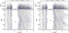 |
Fig. 12 Three-dimensional distributions of dust, for the model represented in Figure 11, displayed at a binary phase around apocenter passage (left) and pericenter passage (right). The positions of the dust are projected in the r-θ plane in the top panels (θs = 0 at the disk mid-plane) and r-ϕ plane. Dust of different sizes are rendered by different colors, as indicated in the legend. The filled gray circles represent the position of the planet. |
6 Conclusions
We use 3D hydrodynamics simulations with Lagrangian particles to analyse the dynamics of gas and dust around the primary star of a close and eccentric binary system, using γ Cephei as a representative case. We consider configurations with and without an embedded giant planet orbiting the primary star.
Contrary to previous results (e.g., Jordan et al. 2021, and references therein), based on 2D simulations (and confirmed herein), we found that 3D models predict low average orbital eccentricities (≲0.03) and slow retrograde precession. We also identify the range of pressure scale-heights in which the transition to prograde precession takes place. These outcomes, which apply to both gas and dust, would be consequential for planetary assembly in the circumprimary disk since they would facilitate accumulation of solids and planetesimal formation.
Models suggest that dust grains, in the range from ~μm to ~mm, remain well coupled to the gas until the gas surface density becomes very small (≲10 g cm−2). Therefore, their dynamics is dictated by that of the gas and the overall distributions of orbital elements are statistically similar across this size range. We also conclude that the planet does not have any significant (large scale) impact on the vertical distribution of dust and only contributes locally to the orbital eccentricity of gas and dust.
As argued by MD25, 3D models also suggest that a compact circumprimary disk has a short lifetime, ~105 years, also due to an enhanced mass transport driven by tidal interactions. In situ formation of a giant planet would require a long-term supply of material from an external source, for example, from a circumbinary disk. Indeed, the presence of a massive planet may provide indirect proof that the binary system was once surrounded by a disk. Under continued supply of material (over a few million years), the model parameters adopted herein would allow for planet growth way beyond the mass of Jupiter, a scenario consistent with some observations (Benedict et al. 2018). Small dust grains would remain largely segregated beyond the outer edge of the gap, possibly leading to the formation of a dense dust ring.
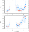 |
Fig. 13 As in Figure 10, but for the model with a giant planet displayed in Figures. 11 and 12. |
Acknowledgements
This work benefited from conversations with Lucas Jordan, Anna Penzlin, and Giovanni Picogna. We thank an anonymous referee for a careful review of this paper. Support from NASA’s Research Opportunities in Space and Earth Science (ROSES) is gratefully acknowledged. Computational resources supporting this work were provided by the NASA High-End Computing Capability (HECC) Program through the NASA Advanced Supercomputing (NAS) Division at Ames Research Center.
References
- Artymowicz, P., & Lubow, S. H. 1994, ApJ, 421, 651 [Google Scholar]
- Baines, E. K., Armstrong, J. T., Schmitt, H. R., et al. 2018, AJ, 155, 30 [Google Scholar]
- Baruteau, C., Crida, A., Paardekooper, S.-J., et al. 2014, in Protostars and Planets VI, eds. H. Beuther, R. S. Klessen, C. P. Dullemond, & T. Henning (Tucson: University of Arizona Press), 667 [Google Scholar]
- Beaugé, C., Leiva, A. M., Haghighipour, N., & Otto, J. C. 2010, MNRAS, 408, 503 [Google Scholar]
- Benedict, G. F., Harrison, T. E., Endl, M., & Torres, G. 2018, Res. Notes Am. Astron. Soc., 2, 7 [Google Scholar]
- Bodenheimer, P., D’Angelo, G., Lissauer, J. J., Fortney, J. J., & Saumon, D. 2013, ApJ, 770, 120 [NASA ADS] [CrossRef] [Google Scholar]
- Campbell, B., Walker, G. A. H., & Yang, S. 1988, ApJ, 331, 902 [NASA ADS] [CrossRef] [Google Scholar]
- Chiang, E., & Youdin, A. N. 2010, Ann. Rev. Earth Planet. Sci., 38, 493 [Google Scholar]
- D’Angelo, G., & Bodenheimer, P. 2013, ApJ, 778, 77 [Google Scholar]
- D’Angelo, G., & Lubow, S. H. 2010, ApJ, 724, 730 [Google Scholar]
- D’Angelo, G., & Marzari, F. 2012, ApJ, 757, 50 [CrossRef] [Google Scholar]
- D’Angelo, G., & Podolak, M. 2015, ApJ, 806, 203 [Google Scholar]
- Duffell, P. C. 2015, ApJ, 807, L11 [CrossRef] [Google Scholar]
- Dullemond, C. P., & Dominik, C. 2004, A&A, 421, 1075 [NASA ADS] [CrossRef] [EDP Sciences] [Google Scholar]
- Endl, M., Cochran, W. D., Hatzes, A. P., & Wittenmyer, R. A. 2011, AIP Conf. Ser., 1331, 88 [Google Scholar]
- Goodchild, S., & Ogilvie, G. 2006, MNRAS, 368, 1123 [NASA ADS] [CrossRef] [Google Scholar]
- Hairer, E., Nørsett, S. P., & Wanner, G. 1993, Solving Ordinary Differential Equations I: Nonstiff Problems, 2nd edn. (Berlin: Springer Series in Computational Mathematics), 8, [Google Scholar]
- Hatzes, A. P., Cochran, W. D., Endl, M., et al. 2003, ApJ, 599, 1383 [NASA ADS] [CrossRef] [Google Scholar]
- Holman, M. J., & Wiegert, P. A. 1999, AJ, 117, 621 [Google Scholar]
- Ida, S., Tanaka, H., Johansen, A., Kanagawa, K. D., & Tanigawa, T. 2018, ApJ, 864, 77 [NASA ADS] [CrossRef] [Google Scholar]
- Jordan, L. M., Kley, W., Picogna, G., & Marzari, F. 2021, A&A, 654, A54 [NASA ADS] [CrossRef] [EDP Sciences] [Google Scholar]
- Kanagawa, K. D., Muto, T., Tanaka, H., et al. 2015, ApJ, 806, L15 [NASA ADS] [CrossRef] [Google Scholar]
- Kanagawa, K. D., Tanaka, H., & Szuszkiewicz, E. 2018, ApJ, 861, 140 [Google Scholar]
- Kley, W., & Nelson, R. P. 2008, A&A, 486, 617 [NASA ADS] [CrossRef] [EDP Sciences] [Google Scholar]
- Liffman, K., & Toscano, M. 2000, Icarus, 143, 106 [Google Scholar]
- Lissauer, J. J., Hubickyj, O., D’Angelo, G., & Bodenheimer, P. 2009, Icarus, 199, 338 [NASA ADS] [CrossRef] [Google Scholar]
- Lubow, S. H. 1992, ApJ, 401, 317 [NASA ADS] [CrossRef] [Google Scholar]
- Lynden-Bell, D., & Pringle, J. E. 1974, MNRAS, 168, 603 [Google Scholar]
- Martin, R. G., Lissauer, J. J., & Quarles, B. 2020, MNRAS, 496, 2436 [Google Scholar]
- Marzari, F., & D’Angelo, G. 2025, A&A, 695, A53 [NASA ADS] [CrossRef] [EDP Sciences] [Google Scholar]
- Marzari, F., Scholl, H., Thébault, P., & Baruteau, C. 2009, A&A, 508, 1493 [NASA ADS] [CrossRef] [EDP Sciences] [Google Scholar]
- Marzari, F., Baruteau, C., Scholl, H., & Thebault, P. 2012, A&A, 539, A98 [NASA ADS] [CrossRef] [EDP Sciences] [Google Scholar]
- Masset, F. 2000, A&AS, 141, 165 [NASA ADS] [CrossRef] [EDP Sciences] [Google Scholar]
- Mugrauer, M., Schlagenhauf, S., Buder, S., Ginski, C., & Fernández, M. 2022, Astron. Nachr., 343, e24014 [NASA ADS] [Google Scholar]
- Müller, T. W. A., & Kley, W. 2012, A&A, 539, A18 [Google Scholar]
- Neuhäuser, R., Mugrauer, M., Fukagawa, M., Torres, G., & Schmidt, T. 2007, A&A, 462, 777 [NASA ADS] [CrossRef] [EDP Sciences] [Google Scholar]
- Picogna, G., & Marzari, F. 2013, A&A, 556, A148 [NASA ADS] [CrossRef] [EDP Sciences] [Google Scholar]
- Pringle, J. E. 1981, ARA&A, 19, 137 [NASA ADS] [CrossRef] [Google Scholar]
- Schwarz, R., Funk, B., Zechner, R., & Bazsó, Á. 2016, MNRAS, 460, 3598 [NASA ADS] [CrossRef] [Google Scholar]
- Silsbee, K., & Rafikov, R. R. 2015, ApJ, 798, 71 [Google Scholar]
- Stone, J. M., & Norman, M. L. 1992, ApJS, 80, 753 [Google Scholar]
- Takeuchi, T., & Lin, D. N. C. 2002, ApJ, 581, 1344 [NASA ADS] [CrossRef] [Google Scholar]
- Thébault, P., Marzari, F., Scholl, H., Turrini, D., & Barbieri, M. 2004, A&A, 427, 1097 [NASA ADS] [CrossRef] [EDP Sciences] [Google Scholar]
- Torres, G. 2007, ApJ, 654, 1095 [NASA ADS] [CrossRef] [Google Scholar]
- Weidenschilling, S. J. 1977, MNRAS, 180, 57 [Google Scholar]
- Whipple, F. L. 1973, NASA Special Publication, 319, 355 [NASA ADS] [Google Scholar]
All Tables
All Figures
|
Fig. 1 Top panels: volume gas density in a vertical slice (r-θ), in units of MA/au3 and logarithmic scale, obtained from a 3D model. The distributions are displayed at a phase of the binary orbit around apocenter passage (left), pericenter passage (center), and shortly thereafter (right). Middle and bottom panels: surface density of the gas, in units of MA/au2 and logarithmic scale, at the same orbital phases as in the top panels, obtained from the 3D model (middle) and from a corresponding 2D model (bottom). |
| In the text | |
|
Fig. 2 Volume gas density in a r-θ plane, in units of MA/au3 and logarithmic scale, from the 3D model of Figure 1. The orbital phase of the binary corresponds to a time ≈0.06 T (top) and ≈0.13 T (middle), after pericenter passage, and ≈0.1 T prior to apocenter passage (bottom). The curves with arrows are streamlines of the gas velocity projected in the r-θ plane (different streamline colors are used to enhance the contrast against the density color-map). The waves excited by the secondary propagate inward, stirring the vertical and radial motion of the gas. |
| In the text | |
|
Fig. 3 Surface density averaged around the primary, in units of MA/au2, obtained from the 3D (red) and 2D (green) models of Figure 1. The thicker curves represent the mean profile computed over an orbital period of the binary, T. The shaded regions indicate maximum and minimum density values attained during the orbit. |
| In the text | |
|
Fig. 4 Mass-weighted disk eccentricity, Eq. (4), of the circumprimary disk versus time. The 2D model predicts an eccentric disk, achieving quasi-equilibrium at ⟨ed⟩ ≈ 0.3 (green circles). The solid line is an average performed every 10 T. In comparison, the 3D model predicts a much less eccentric circumprimary disk (orange circles), ⟨ed⟩ ≈ 0.03. The red curve represents an average over 10 T intervals. |
| In the text | |
|
Fig. 5 Mass-weighted argument of pericenter of the circumprimary disk versus time. The top panel shows results for a 2D (green circles) and a 3D model (orange circles). The 2D model predicts a retrograde precession of the circumprimary disk at a rate of about 6 binary periods for a full revolution. The precession rate resulting from the 3D model is still retrograde, but orders of magnitude slower. The long-term behavior of the 3D model is displayed in the bottom panel. The solid line represent an average over 10 T intervals. See text for further details. |
| In the text | |
|
Fig. 6 Top panels: volume gas density in vertical slices, in units of MA/au3 and logarithmic scale, obtained from a 3D model that includes a giant planet. Each slice passes through the planet location. The distributions are displayed at a binary phase around apocenter passage (left), pericenter passage (center), and shortly thereafter (right). Bottom panels: surface density of the gas, in units of MA/au2 and logarithmic scale, plotted at the same orbital phases as in the top panels. |
| In the text | |
|
Fig. 7 Surface density averaged around the primary, in units of MA/au2, obtained from the 3D model of Figure 6. The density profiles correspond to orbital phases of the binary at apocenter (red) and pericenter (blue). The shaded region represents the surface density of the 3D model without a planet shown in Figure 3. The density peaks inside the tidal gap generated by the planet indicate the radial position of the planet (which moves on an eccentric orbit). |
| In the text | |
|
Fig. 8 Integration of the planet mass according to the accretion rates reported in Lissauer et al. (2009) and Bodenheimer et al. (2013), assuming that the circumprimary disk is supplied by the circumbinary disk with an initial accretion rate dMcb/dt as indicated, in units of M⊙ yr−1 (see MD25). The supply rate declines to zero over the circumbinary disk lifetime, a few million years in this example. See text for further details. |
| In the text | |
|
Fig. 9 Histograms of dust orbital properties obtained from a 3D model without a giant planet. Semi-major axis (left), eccentricity (center), inclination (right) of the solids are displayed at a binary phase around apocenter passage (top) and pericenter passage (bottom). Histograms are stacked in order of increasing dust size, as indicated in the legends. |
| In the text | |
|
Fig. 10 Average orbital eccentricity of 1 μm-size dust, as function of semi-major axis, corresponding to the orbital phases of the binary of apocenter (top) and pericenter passage (bottom). Red symbols refer to grains within one scale-height H of the disk mid-plane whereas blue symbols refer to grains moving above H. Error bars provide the spread (standard deviation) of the distributions around the mean values. |
| In the text | |
|
Fig. 11 Histograms of dust orbital properties as in Figure 9, but for a model that contains a giant planet. Top and bottom panels display distributions at a binary phase around apocenter and pericenter passage, respectively. Histograms are stacked in order of increasing dust size, as indicated. The enhanced concentrations around 2–2.1 au in the left panels correspond to particles orbiting the planet. The narrow high peaks in the eccentricity distributions are generated by grains that move along the edges of the tidal gap opened by the planet (see also bottom panels of Figure 12). |
| In the text | |
|
Fig. 12 Three-dimensional distributions of dust, for the model represented in Figure 11, displayed at a binary phase around apocenter passage (left) and pericenter passage (right). The positions of the dust are projected in the r-θ plane in the top panels (θs = 0 at the disk mid-plane) and r-ϕ plane. Dust of different sizes are rendered by different colors, as indicated in the legend. The filled gray circles represent the position of the planet. |
| In the text | |
|
Fig. 13 As in Figure 10, but for the model with a giant planet displayed in Figures. 11 and 12. |
| In the text | |
Current usage metrics show cumulative count of Article Views (full-text article views including HTML views, PDF and ePub downloads, according to the available data) and Abstracts Views on Vision4Press platform.
Data correspond to usage on the plateform after 2015. The current usage metrics is available 48-96 hours after online publication and is updated daily on week days.
Initial download of the metrics may take a while.