| Issue |
A&A
Volume 702, October 2025
|
|
|---|---|---|
| Article Number | A56 | |
| Number of page(s) | 41 | |
| Section | Interstellar and circumstellar matter | |
| DOI | https://doi.org/10.1051/0004-6361/202452986 | |
| Published online | 07 October 2025 | |
Multi-frequency analysis of the ALMA and VLA high resolution continuum observations of the substructured disc around CI Tau
Preference for submillimetre-sized low-porosity amorphous carbon grains
1
Max Planck Institute for Astronomy,
Königstuhl 17,
69117
Heidelberg,
Germany
2
Institute of Astronomy, University of Cambridge,
Madingley Road,
Cambridge
CB3 OHA,
UK
3
Università degli Studi di Milano,
Via Giovanni Celoria 16,
20133
Milano,
Italy
4
European Southern Observatory,
Karl-Schwarzschild-Str. 2,
85748
Garching bei München,
Germany
5
Departamento de Astronomía, Universidad de Chile,
Camino El Observatorio 1515, Las Condes,
Santiago,
Chile
6
Institute for Astronomy, University of Hawaii,
Honolulu,
HI
96822,
USA
7
INAF – Osservatorio Astrofisico di Arcetri,
L.go E. Fermi 5,
50125
Firenze,
Italy
8
Astrophysics Group, Department of Physics, Imperial College London,
Prince Consort Rd,
London
SW7 2A2,
UK
9
School of Physics and Astronomy, University of Leeds,
Leeds
LS2 9JT,
UK
10
Leiden Observatory, Leiden University,
PO Box 9513,
2300
RA
Leiden,
The Netherlands
11
School of Physics & Astronomy, University of Leicester,
University Road,
Leicester
LE1 7RH,
UK
12
Dipartimento di Fisica e Astronomia, Università di Bologna,
Via Gobetti 93/2,
40122
Bologna,
Italy
★ Corresponding author: This email address is being protected from spambots. You need JavaScript enabled to view it.
Received:
13
November
2024
Accepted:
10
July
2025
Abstract
We present high angular resolution (50 mas) and sensitivity Atacama Large Millimeter/submillimeter Array (ALMA) Band 3 (3.1 mm) and Very Large Array (VLA) Ka band (9.1 mm) observations of the multi-ringed disc around the 3 Myr-old solar-mass star CI Tau. These new data were combined with similar-resolution archival ALMA Band 7 (0.9 mm) and 6 (1.3 mm) observations and new and archival VLA Q (7.1 mm), Ku (2.0 cm), X (3.0 cm), and C band (6.0 cm) photometry to study the properties of dust in this system. At wavelengths ≤3.1 mm, the continuum emission from CI Tau is very extended (≥200 au) and highly substructured (with three gaps, four rings, and two additional gap-ring pairs identified by non-parametric visibility modelling). In contrast, the VLA Ka band data are dominated by a centrally peaked bright component, only partially (≤50%) due to dust emission, surrounded by a marginally detected faint and smooth halo. We fitted the ALMA and VLA Ka band data together, adopting a physical model that accounts for the effects of dust absorption and scattering. For our fiducial dust composition (‘Ricci’ opacities), we retrieved a flat maximum grain size distribution across the disc radius, with amax = (7.1 ± 0.8) × 10−2 cm that we tentatively attributed to fragmentation of fragile dust or bouncing. We tested, for the first time, the dependence of our results on the adopted dust composition model to assess which mixture can best reproduce the observations. We found that ‘Ricci’ opacities work better than the traditionally adopted ‘DSHARP’ ones, while graphite-rich mixtures perform significantly worse. We also show that for our fiducial composition, the data prefer low porosity (≤70%) grains. This is in contrast with recent claims of highly porous aggregates in younger sources, which we tentatively justified by time-dependent compaction at the fragmentation or bouncing barrier. Our results on composition and porosity are in line with constraints from disc population synthesis models and naturally arise from CI Tau’s peculiar spectral behaviour (i.e. the abrupt steepening of its spectral index at wavelengths longer than 3.1 mm), making this disc a unique target to characterise the properties of disc solids and thus ideal for deeper centimetre-wavelength observations and follow-up dust polarisation studies.
Key words: radiative transfer / methods: data analysis / techniques: interferometric / planets and satellites: formation / protoplanetary disks / stars: individual: CI Tauri
© The Authors 2025
 Open Access article, published by EDP Sciences, under the terms of the Creative Commons Attribution License (https://creativecommons.org/licenses/by/4.0), which permits unrestricted use, distribution, and reproduction in any medium, provided the original work is properly cited.
This article is published in open access under the Subscribe to Open model.
Open Access funding provided by Max Planck Society.
1 Introduction
Dust is an essential ingredient of every planet-formation model. First and foremost, it is the material planet(esimal)s are made of. By dominating the disc opacity, solids also set the temperature structure and thus the excitation conditions and reaction rates of volatiles (e.g. Gavino et al. 2021; Öberg et al. 2023). In addition, electron-ion recombination and chemical reactions on the surface of grains affect the disc ionisation structure (e.g. Desch & Turner 2015) and prompt the formation of complex organic molecules (e.g. Öberg & Bergin 2021). Dust collisional evolution (growth and fragmentation) and transport (vertical settling and radial drift) not only determine the availability of solids to form planetary cores (Brauer et al. 2008; Birnstiel et al. 2010) but also affect the dust-to-gas thermal coupling (Facchini et al. 2017) and the abundance of gas-phase chemical species. As dust migrates radially, the volatiles frozen onto grains undergo thermal desorption upon transition across their snowlines (e.g. Booth et al. 2017; Booth & Ilee 2019; Krijt et al. 2020; Van Clepper et al. 2022), thus locally enriching the feedstock of exoplanet atmospheres (Madhusudhan 2019). Therefore, unsurprisingly, determining the physical and chemical properties of protoplanetary disc solids is an essential first step to understanding planet formation (e.g. Miotello et al. 2023; Birnstiel 2024). For this reason, attempts have been made to infer the density, size, distribution, and temperature of disc solids by modelling the continuum emission from planet-forming discs at multiple wavelengths.
Early works, which either focused on a few targets of interest or surveyed tens of discs in nearby star-formation regions, measured integrated spectral indices, first in the (sub-)millimetre and then at progressively longer wavelengths significantly smaller than in the interstellar medium (ISM). While the contribution of optically thick regions could not be ruled out (Ricci et al. 2012), especially at (sub-)millimetre wavelengths, these results were generally interpreted (Beckwith & Sargent 1991; Andrews & Williams 2005; Rodmann et al. 2006), sometimes in combination with information on the (wavelength dependence of the) disc radius (e.g. Testi et al. 2003; Wilner et al. 2005; Ricci et al. 2010a,b; Isella et al. 2010; Banzatti et al. 2011; Guilloteau et al. 2011), as being a consequence of substantial grain growth up to millimetre or centimetre sizes, depending on the adopted dust optical properties (see Testi et al. 2014 and Andrews 2020 for a summary picture). In addition, the first multi-wavelength studies able to resolve a few bright sources from (sub-)millimetre to centimetre wavelengths (Pérez et al. 2012, 2015; Trotta et al. 2013; Tazzari et al. 2016) inferred radially decreasing grain size profiles, in qualitative agreement with the predictions of dust evolution models (Brauer et al. 2008; Birnstiel et al. 2010).
The advent of the Atacama Large Millimeter/submillimeter Array (ALMA) substantially revolutionised this picture. One of ALMA’s major breakthroughs was the almost ubiquitous detection of small scale structures in the continuum emission of (the largest and brightest) protoplanetary discs (Andrews 2020; Bae et al. 2023). At (sub-)millimetre wavelengths, substructures are most commonly detected in the form of axisymmetric troughs and peaks (colloquially referred to as ‘gaps’ and ‘rings’; e.g. Andrews et al. 2016; Long et al. 2018; Andrews et al. 2018; Huang et al. 2018b) or cavities (e.g. Keppler et al. 2019; Facchini et al. 2020), but spirals (Pérez et al. 2016; Huang et al. 2018c; Kurtovic et al. 2018; Paneque-Carreño et al. 2021) and crescents (e.g. van der Marel et al. 2013; Isella et al. 2018; Pérez et al. 2018; Dong et al. 2018) are sometimes also present. On the one hand, the most tantalising interpretation of these structures is that they trace dynamical interactions between massive (0.1 to 10.0 MJup, Lodato et al. 2019; Bae et al. 2023; Ruzza et al. 2024) protoplanets and their hosting disc (e.g. Zhang et al. 2018). However, despite many attempts using infrared (IR) high-contrast imaging (e.g. Testi et al. 2015; Guidi et al. 2018), photospheric emission of accreting planets was detected only in one case (PDS 70, e.g. Keppler et al. 2018; Haffert et al. 2019). On the other hand, a plethora of alternative mechanisms have been put forward to explain the wealth of observed substructures (e.g. Bae et al. 2023), such as (magneto-)hydrodynamic instabilities (Lesur et al. 2023 and references therein), thermal and magnetic winds (Pascucci et al. 2023 and references therein), eccentric modes (sometimes triggered by gravitationally bound companions or flybys, e.g. Ragusa et al. 2017; Cuello et al. 2023), or physical-chemical processes that alter the properties of dust at the snowlines of the major volatile species (e.g. Zhang et al. 2015; Okuzumi et al. 2016).
Determining the properties of disc substructures, such as dust density and size (see below), gap-to-ring contrast (Huang et al. 2018b), and trapping ability (Dullemond et al. 2018; Rosotti et al. 2020; Doi & Kataoka 2023), is of paramount importance. This is crucial not only to discriminate between their possible origins (Bae et al. 2023) but also to assess their potential to form (second generation, see the discussion of Bae et al. 2023) planet(esimal)s by streaming instability (Youdin & Goodman 2005; Johansen et al. 2007, see Carrera et al. 2021, 2022; Xu & Bai 2022 for the specific case of pressure bumps) or gravitational instability (Goldreich & Ward 1973) and the subsequent growth by pebble accretion (Lau et al. 2022; Jiang & Ormel 2023).
The substructured discs observed with ALMA at high angular resolution (e.g. Andrews et al. 2018) showed clear indications of moderate-to-high absorption optical depths in the inner regions and at the position of the bright rings (Huang et al. 2018b; Dullemond et al. 2018), which is considered to be an indication of unresolved optically thick substructures (Dullemond et al. 2018), self-regulating planetesimal formation (Stammler et al. 2019), or high extinction in the presence of self-scattering by highly reflective grains (e.g. Zhu et al. 2019, although Isella et al. 2018 and Guzmán et al. 2018 showed that dust rings do not completely suppress line emission). The spectral index radial profile modulations at the position of gaps and rings inferred from high angular resolution multi-frequency continuum observations (e.g. ALMA Partnership 2015; Tsukagoshi et al. 2016; Macías et al. 2019; Huang et al. 2020a) and the ‘anomalously low’ (i.e. α < 2) spectral indices in the innermost regions of a few sources (e.g. Huang et al. 2018a; Dent et al. 2019; Paneque-Carreño et al. 2021; Ribas et al. 2023; Houge et al. 2024), which are most often attributed to dust self-scattering (Liu 2019), go well in line with this picture of moderate-to-high optical depths in the inner disc and the bright rings. These clues suggest that the classically adopted assumption of optically thin continuum emission is rather inaccurate when analysing (sub-)millimetre observations and leads to overestimation of the grain size and underestimation of the dust density (e.g. Zhu et al. 2019; Carrasco-González et al. 2019).
Broadband high angular resolution multi-frequency continuum observations with ALMA (Macías et al. 2021; Sierra et al. 2021; Maucó et al. 2021; Ueda et al. 2022; Ohashi et al. 2023; Carvalho et al. 2024; Sierra et al. 2025), complemented with Very Large Array (VLA) data in some cases (Carrasco-González et al. 2019; Guidi et al. 2022; Zhang et al. 2023; Sierra et al. 2024; Guerra-Alvarado et al. 2024), allowed the degeneracies between intrinsic dust properties and the wavelength dependence of the optical depth to be broken, thus opening up the possibility of thoroughly characterising the temperature, density, and size of solids in gaps and rings. Not surprisingly, most of these works obtained rather different constraints. While partly due to the intrinsic diversity of the analysed sources, the different modelling hypotheses (e.g. the adopted dust composition and porosity or the fitting methods) might have impacted their results substantially. In this paper, we combine ALMA and VLA high angular resolution and sensitivity (sub-)millimetre continuum observations and centimetre-wavelength photometry of CI Tau (whose stellar parameters are summarised in Table K.1) to provide constraints on the properties of solids and simultaneously explore different assumptions on dust composition and porosity.
1.1 The case of CI Tau
CI Tau is the youngest pre-main-sequence star where periodic variability in multi-epoch IR radial velocity measurements, also supported by optical spectroscopy and photometric monitoring, was attributed to a moderately eccentric (0.28 ± 0.16) massive (11.29 ± 2.13 MJup) candidate planet on a nine-day period orbit (Johns-Krull et al. 2016). This claim was further backed by the detection of a similar-period variability in K2 (the extended mission of the Kepler Space Telescope) photometry (Biddle et al. 2018, 2021), consistent with accretion modulation on the planet’s orbital period (see Teyssandier & Lai 2020), and of CO emission, proposed to be associated with the candidate hot Jupiter (Flagg et al. 2019).
Since the in situ formation of this candidate planet was considered unlikely (see Rosotti et al. 2017 and references therein), planet migration and interactions with or scattering by an unseen companion were put forward as possible explanations for the origin of this hot Jupiter. On the one hand, while early simulations suggested that the planet eccentricity can be pumped up while migrating in a low-mass disc over long timescales (Rosotti et al. 2017; Ragusa et al. 2018), it was recently shown that type II migration preferably leads to the pile-up of planets between 1 and 10 au, precluding the formation of hot Jupiters by migration in a (non-self-gravitating) disc (Scardoni et al. 2022). On the other hand, high-contrast IR angular differential imaging ruled out the presence of companions more massive than 2 to 4 MJup external to 30 au (Shimizu et al. 2023), in line with the prediction that eccentricity-driving lower-mass companions are ejected or accreted after dynamical interactions (Rosotti et al. 2017).
Most recently, (sub-)au resolution VLTI/GRAVITY observations (GRAVITY Collaboration 2023) revealed that CI Tau’s inner disc emission is non-axisymmetric, in line with the predictions of planet-disc interaction simulations (e.g. Muley & Dong 2021), and misaligned by ≈70° with the outer disc (see Clarke et al. 2018), potentially due to the gravitational torque induced by a massive close-in companion. Moreover, the inner dust disc rim is located two to four times further out than the expected position of the sublimation radius, as expected from the presence of an inner companion carving a gap in the disc (Muley & Dong 2021). This hypothesis was further supported by the shape of the CO ν = 1–0 ro-vibrational transitions targeted by IRTF/iSHELL and Keck/NIRSPEC (Kozdon et al. 2023). These lines show a blueshifted core and redshifted wings, that can be explained by two eccentric disc components with oppositely aligned arguments of periapsis, separated by a massive eccentric planet, albeit with much lower eccentricity (≈0.05) than estimated by Johns-Krull et al. (2016).
However, the spectro-polarimetric monitoring of CI Tau with ESPaDOnS and SPIRou/CFHT (Donati et al. 2020, 2024) recently showed that the nine-day periodicity detected by Johns-Krull et al. (2016) is most-likely driven by the stellar rotation, and the CO emission detected by Flagg et al. (2019) might be connected to the accretion funnels onto the star, thus suggesting that the presence of a hot Jupiter in the system needs to be reconsidered. Likewise, the most recent detection of a 25.2-day periodicity in ESPaDOnS and SPIRou/CFHT multi-epoch radial velocity monitoring, as well as K2 and LCOGT photometric time series, attributed to a highly eccentric (0.58 ± 0.05) massive (3.6 ± 0.3 MJup) planet (Manick et al. 2024), was disputed by Donati et al. (2024), who proposed that it can be explained by an asymmetry in the inner disc. Whether the disc around CI Tau hosts a hot Jupiter or not remains debated.
Being bright and large at (sub-)millimetre wavelengths, CI Tau was extensively targeted in the pre-ALMA era, both in single dish (e.g. Beckwith et al. 1990; Beckwith & Sargent 1991; Andrews & Williams 2005) and interferometric observations (e.g. Dutrey et al. 1996; Andrews & Williams 2007; Andrews et al. 2013; Kwon et al. 2015). Early multi-wavelength analyses measured a millimetre spectral index of α1.3–2.7 mm = 2.5 ± 0.2 (Dutrey et al. 1996; Ricci et al. 2010b; Guilloteau et al. 2011) that steepens to α1.3–7.0 mm = 3.0 ± 0.3 at longer wavelengths (Rodmann et al. 2006), and a ![Mathematical equation: $\[\beta_{1.3-2.7 \mathrm{~mm}}^{\text {abs}}\]$](/articles/aa/full_html/2025/10/aa52986-24/aa52986-24-eq1.png) profile radially increasing between ≲ 0.5 and ≳ 1.0 (see Figures 10 and 11 of Guilloteau et al. 2011).
profile radially increasing between ≲ 0.5 and ≳ 1.0 (see Figures 10 and 11 of Guilloteau et al. 2011).
High-angular resolution and sensitivity ALMA observations of CI Tau at 1.3 mm revealed a very extended (≥200 au) disc characterised by a sequence of four rings and three gaps, compatible with the presence of three 0.75, 0.15, and 0.40 MJup planets in the system (Clarke et al. 2018; Long et al. 2018), or the snowlines of CO and clathrate-hydrated CO and N2 for the two innermost gaps (Long et al. 2018). Adopting a super-resolution imaging technique, Jennings et al. (2022b) identified two additional gaps, making CI Tau one of the most substructured discs observed to date, together with AS 209 (Guzmán et al. 2018), HL Tau (ALMA Partnership 2015), TW Hya (Andrews et al. 2016), HD 163296 (Isella et al. 2018), and RU Lup (Huang et al. 2020b). Follow-up observations at 0.9 mm showed a similar continuum morphology (Rosotti et al. 2021). On the contrary, the scattered light emission in SPHERE polarimetric images shows no substructures, but a bright ≈100 au inner disc surrounded by a faint halo extending to ≳ 200 au (Garufi et al. 2022).
As for the lines, although both 12CO J = 2–1 and J = 3–2 emission is heavily absorbed towards CI Tau (Rosotti et al. 2021; Semenov et al. 2024), a kinematic planetary signature external to the dusty disc was proposed in one of the non-absorbed channels (Rosotti et al. 2021). Instead, 13CO J = 2–1 and J = 3–2 emission is not absorbed. When observed at high-angular resolution, the latter shows a low-contrast gap co-located with the ≈60 au continuum ring, attributed by Rosotti et al. (2021) to shadowing by the inner disc. A shallow dip in the 12CO J = 3–2 emission height at the same position of the ≈50 au gap, and a change of slope co-located with the ≈100 au ring, were detected by Law et al. (2022). Similarly, the 12CO temperature profile shows two dips at ≈70 and ≈120 au and a bump at ≈90 au co-located with similar features in the continuum and 13CO J = 3–2 emission (Law et al. 2022). The CS J = 7–6 emission is ring-like, while the J = 5–4 one is smooth, most likely due to chemical effects (e.g. Le Gal et al. 2019; Rosotti et al. 2021). CCH N = 3–2 and C18O J = 2–1 emission are relatively bright and centrally peaked (Bergner et al. 2019; Semenov et al. 2024).
This paper is organised as follows. In Section 2 we introduce our datasets, discuss their (self-)calibration and imaging. CI Tau’s (integrated and resolved) spectral properties are discussed in Section 3. In Section 4 we introduce our analysis procedure, while in Section 5 we present our results, that are discussed in Section 6. In Section 7 we draw our conclusions.
2 Observations, calibration, and imaging
2.1 Observations
We introduce, for the first time, ALMA Band 3, VLA Ka, Ku, X, and C band observations of CI Tau. We make use of archival ALMA Band 6 (Konishi et al. 2018; Clarke et al. 2018) and 7 (Rosotti et al. 2021) observations to study the properties of solids in this disc at high angular resolution and sensitivity. Information about these datasets is summarised in Table K.2.
ALMA Band 3 observations. ALMA Band 3 observations were conducted in Cycle 6 and 7 between June 2019 and July 2021 as part of the program 2018.1.00900.S (PI: M. Tazzari). The data were correlated from four spectral windows (SPWs) in dual polarisation mode. All the SPWs were set in frequency division mode (FDM), each with 1920 channels 976.562 kHz wide, spanning a total bandwidth of 1.875 GHz, and centred at 90.5, 92.5, 102.6, and 104.5 GHz. The target was observed in the more compact C43-6 configuration (short baselines, SBs), and the more extended C43-9 configuration (long baselines, LBs).
The SB observations used an array with baseline lengths from 15.3 m to 2.4 km (≈400 mas resolution) and 41 antennas. The total integration time on the science target was ≈38 min. The phase calibrator J0426+2327 was observed in an alternating sequence with the science target, every 10 min. The bandpass and flux calibrator J0237+2848 was observed at the beginning of the observing block. The LB observations used an array with baseline lengths from 83.1 m to 16.2 km (≈50 mas resolution). Two execution blocks (EBs) were scheduled. The first used 42 antennas and the second 46. The total integration time on the science target was ≈44 min for each EB. The phase calibrator J0426+2327 was observed in an alternating sequence with the science target, every minute. The bandpass and flux calibrator, J0423–0120 and J0510+1800 for different EBs, respectively, was observed at the beginning of the observing block. An additional ‘check’ calibrator, J0425+2235, was observed every ≈15 min to assess the quality of phase transfer.
ALMA Band 6 observations. The publicly available archival ALMA Band 6 observations (that we took into account) were conducted in Cycle 3 in August 2016 as part of the program 2015.1.01207.S (PI: H. Nomura) and in Cycle 4 in September 2017 as part of the program 2016.1.01370.S (PI: C. J. Clarke). The data were correlated from four SPWs in dual polarisation mode. For the program 2016.1.01370.S, all the SPWs were set in time division mode (TDM), each with 128 channels 15.625 MHz wide, spanning a total bandwidth of 2.0 GHz, and centred at 224.0, 226.0, 240.0, and 242.0 GHz. Instead, for the program 2015.1.01207.S, the SPWs were set in FDM and centred at: (i) 220.0 GHz with a bandwidth of 234.0 MHz in 480 channels of 488.3 kHz; (ii–iii) 216.7 and 231.2 GHz with a bandwidth of 937.5 MHz in 1920 channels of 488.3 kHz; (iv) 234.4 GHz with a bandwidth of 937.5 MHz in 960 channels of 976.6 kHz.
The 2016.1.01370.S program observations were scheduled in two EBs, both relied on an array with baseline lengths from 41.4/21.0 m to 12.1 km (≈35 mas resolution) in the C40-8/9 configuration (LBs). The first EB used 40 antennas and the second 41. The total integration time on the science target was ≈33 min for each EB. The phase calibrator J0426+2327 was observed in an alternating sequence with the science target, every minute. The bandpass and flux calibrator J0510+1800 was observed at the beginning of the observing block. An additional “check” calibrator J0438+2153 was observed every ≈12 min.
The 2015.1.01207.S program observations used an array with baseline lengths from 15.1 m to 1.6 km (≈250 mas resolution) and 44 antennas in the C40-6 configuration (SBs). The total integration time on the science targets was ≈18 min (half of which on CI Tau). The phase calibrator J0431+2037 was observed in an alternating sequence with the science targets, every 6 min. The bandpass and flux calibrator J0510+1800 was observed at the beginning of the observing block.
ALMA Band 7 observations. ALMA Band 7 observations were conducted in Cycle 5 in December 2017 as part of the DDT program 2017.A.00014.S (PI: G. P. Rosotti). The data were correlated from four SPWs in dual polarisation mode. Three SPWs were set in FDM each with 1920 channels 448.3 kHz-wide centred at 330.7, 343.0, and 345.7 GHz, and spanning a total bandwidth of 937.5 MHz. The remaining SPW, centred at 333.2 GHz, was set in TDM, with 128 channels 15.625 MHz-wide, and spanning a total bandwidth of 2 GHz. The observations used an array with baseline lengths from 15.1 m to 3.3 km (≈90 mas resolution) and 43 antennas in the C43-7 configuration. Two EBs were scheduled. The total integration time on the science target was ≈39 min for each EB. The phase calibrator J0426+2327 was observed in an alternating sequence with the science target, every minute. The bandpass and flux calibrator J0510+1800 was observed at the beginning of the observing block. An additional “check” calibrator J0435+2532 was observed every ≈13 min to assess the quality of phase transfer.
VLA Ka, Ku, X, and C band observations. CI Tau was observed by the VLA in Ka band in two configurations as part of the project 19A-440 (PI: M. Tazzari). The SPWs covered the frequency range between 29 and 37 GHz (wavelengths between 8.1 and 10.3 mm). Observations in B configuration, with a maximum baseline of 11.1 km, were performed during March and April 2019 and September and October 2020, for a total on-source integration time of 9.8 h. Observations in A configuration, with a maximum baseline of 36.6 km, were executed between September and October 2019, resulting in a total on-source integration time of 8.6 h. For both configurations, 3C147 served as the flux and bandpass calibrator, J0403+2600 was used for pointing calibration, and J0431+2037 for phase calibration.
Under the same VLA project 19A-440, X band observations in A configuration (maximum baseline of 36.6 km) were conducted in August 2019, for a total integration time on the science target of 1.3 h. The bandwidth extended from 8 to 12 GHz (corresponding to wavelengths from 2.5 to 3.7 cm). 3C147 was used for flux and bandpass calibration, J0403+2600 for phase calibration, while no pointing calibrator was observed.
As part of the VLA project 20A-373 (PI: M. Tazzari), CI Tau was observed in the Ku and C band, both in C configuration, with a maximum baseline of 3.4 km. Ku band observations were performed between February and March 2020, with a spectral coverage from 12 to 18 GHz (1.7 to 2.5 cm), for a total on-source integration time of 44.5 min. C band observations were carried out in 2020, with a bandwidth from 4 to 8 GHz (3.7 to 7.5 cm), and a total on-source integration time of 14.9 min. For both bands, 3C147 was employed for the flux and bandpass calibration, while J0431+2037 for the phase calibration. J0431+2037 also served as pointing calibrator for Ku band, whereas C band did not require any pointing calibration.
2.2 (Self-)calibration
The standard pipeline calibration was performed manually for ALMA Band 3, Band 6 SB and the VLA observations. The other datasets were pipeline-calibrated by the European ARC at ESO. Self-calibration was performed using the software CASA (Common Astronomy Software Applications, McMullin et al. 2007; CASA Team 2022) v6.4.3.27 for ALMA observations (ex novo also for the archival Band 6 and 7 data) and v6.2.1.7 for the VLA data, as explained hereafter.
ALMA observations. We followed the standard methodology adopted by the DSHARP collaboration (Andrews et al. 2018), with some minor changes. To begin with, channel-averaging was performed ensuring the same number of channels per SPW in each EB. To avoid bandwidth smearing, we adopted the criterion of Bridle & Schwab (1989) for a reduction of <1% in peak response to a point source at the edge of the primary beam. For Band 7, a pseudo-continuum measurement set (MS) was first created, flagging data within −5 ≤ v/(km s−1) ≤ 15 (to account for CI Tau’s systematic velocity) of the 13CO J = 3–2 (ν0 = 330.588 GHz), CS J = 7–6 (ν0 = 342.883 GHz), and 12CO J = 3–2 (ν0 = 345.796 GHz) molecular line transition centres.
When available, the SB data were self-calibrated first, initially in phase-only mode. The gain solutions were computed using the task gaincal1. For the first run, this was done separately for each polarisation (gaintype=‘G’) for Band 3 and combining both polarisations (gaintype=‘T’) for Band 6, combining different scans, with an infinite solution interval. From the second run on, for both Band 3 and 6 data, the gain solutions were computed with gaintype=‘T’, combining different scans and spectral windows, with solution intervals progressively decreasing from 240, 120, 60, 30, to 15 s. Images were reconstructed after each iteration using the tclean task. We set the CLEANing threshold to three times the noise level, used 10 pixels per beam, a multi-scale multi-frequency synthesis deconvolver (mtmfs, see Rau & Cornwell 2011) with nterms=2, and adopted a briggs weighting scheme (Briggs 1995) with robust=0.5. We estimated an improvement of the peak signal-to-noise ratio (S/N) of ≈ 28% and ≈ 40% for Band 3 and Band 6 data, respectively. Finally, a round of phase and amplitude self-calibration was performed. The gain solutions were computed with gaintype=‘T’, combining different scans and spectral windows, with an infinite solution interval. However, we did not observe any improvement of the peak S/N (as already reported by Konishi et al. 2018 for Band 6 data).
Then, all the EBs in the same band were concatenated and self-calibrated together. To remove spatial offsets, we measured the emission centroid positions of each dataset with a Gaussian fit in the image plane. Subsequently, the phaseshift task was used to move the disc centre to the fitted phase centre position, and the fixplanets task to align each EB to the phase centre of the LBs with the highest peak S/N (i.e. the EB with the smallest astrometric uncertainty and lowest noise). Before these steps, we performed a run of phase-only self-calibration on the LB data to increase their peak S/N ratio. The gain solutions were computed with gaintype=‘G’, combining different scans with an infinite solution interval. This additional step helped to improve the alignment procedure. Subsequently, the visibilities of each dataset were deprojected and azimuthally averaged. To do so, we used the median of the posterior distribution of the inclination (i = 49.24 deg) and position angle (PA = 11.28 deg) that Clarke et al. (2018) determined by fitting the Band 6 LB data in the Fourier space parametrically with galario (Tazzari et al. 2018). These deprojected visibilities were then inspected to identify and correct for mismatches in the amplitude scales. This step is crucial to ensure an accurate flux scaling with wavelength, and proved to be particularly important for Band 6 data, where flux density variations larger than 10% over a single day were measured. We refer to Appendix A for a detailed discussion of our correction procedure, and the time variability of the flux calibrators.
The short and long baseline data in the same ALMA bands were then combined using the concat task. We performed a number of phase-only self-calibration iterations on the concatenated MS. For the first run, the gain solutions were computed with gaintype=‘G’ for Band 3 and 7, and gaintype=‘T’ for Band 6, combining different scans with an infinite solution interval. From the second run on, the gain solutions were computed with gaintype=‘T’, combining different scans and spectral windows, with solution intervals progressively decreasing from 360, 180, to 60 for Band 3, and to 30 and 15 s for Band 6 and 7. Image reconstruction was performed as for the SBs, but with robust=1.0. We estimated an improvement of the peak S/N of ≈ 21% for Band 6, ≈ 26% for Band 7, and only marginal for Band 3. Finally, we performed a round of phase and amplitude self-calibration with gaintype=‘T’, combining different scans and spectral windows with an infinite solution interval. We flagged the most extreme gain solutions (with gains <0.8 or >1.2), that are associated with long-baseline antennas and artificially reduced the beam size. After this iteration, the peak S/N ratio improved substantially only in Band 7 by an additional factor of ≈ 20% (i.e. a total improvement by 56%).
VLA observations. We conducted spectral averaging on each dataset, considering the necessary precautions to prevent bandwidth smearing2. Time averaging was not performed. In the imaging process, we adopted a briggs weighting scheme with robust=1.0, representing the optimal trade-off between S/N and side lobe effects. The mtmfs deconvolver with nterms=2 was employed to accurately account for the large bandwidth-over-observing-frequency ratio in the VLA data.
For the Ka band observations, we initially aligned the data from different EBs to ensure that the disc centre was consistent across all the datasets. Then, we applied a single round of phase-only self-calibration only to the B configuration (lower angular resolution) data, leading to a slight improvement of the peak S/N by ≈ 5%. We adopted the following gaincal parameters: gaintype=‘G’, combine=‘scan’, solint=‘inf’. Subsequently, the B configuration data were combined with the A configuration (higher angular resolution) ones. Similarly, a round of phase-only self-calibration was performed, resulting in a further increase in the peak S/N by ≈ 10%. Additional self-calibration iterations with shorter solution intervals did not yield any further improvement. For the Ku band data, we applied one round of phase-only self-calibration (again with gaintype=‘G’, combine=‘scan’, solint=‘inf’) resulting in a marginal improvement of the S/N by ≈ 10%. Due to the initially (too) low S/N, no self-calibration was performed on the X and C band data to avoid introducing spurious effects.
2.3 Fiducial images and radial profiles
We reconstructed the ALMA and VLA Ka band fiducial images CLEANing over an elliptical mask with a semi-major axis of ![Mathematical equation: $\[1^{\prime\prime}_\cdot5\]$](/articles/aa/full_html/2025/10/aa52986-24/aa52986-24-eq2.png) , a semi-minor axis of
, a semi-minor axis of ![Mathematical equation: $\[0^{\prime\prime}_\cdot9\]$](/articles/aa/full_html/2025/10/aa52986-24/aa52986-24-eq3.png) , and PA = 11.28 deg (Clarke et al. 2018), down to the estimated noise level (i.e. a 1σ RMS noise threshold), using 8 pixels per beam semi-minor axis. Different robust parameters were tested, progressively increasing by 0.5 from −1.0 to 1.5. We adopted a mtmfs deconvolver with nterms=2, and a set of (Gaussian) deconvolution scales (Cornwell 2008), different for each band and robust parameter, including a point source, scales corresponding to one and two beams, and, for ALMA data, to the ring locations (from Clarke et al. 2018), and the outer disc radius. The image noise was estimated over a circular annulus centred on and larger than the target with inner and outer radius of
, and PA = 11.28 deg (Clarke et al. 2018), down to the estimated noise level (i.e. a 1σ RMS noise threshold), using 8 pixels per beam semi-minor axis. Different robust parameters were tested, progressively increasing by 0.5 from −1.0 to 1.5. We adopted a mtmfs deconvolver with nterms=2, and a set of (Gaussian) deconvolution scales (Cornwell 2008), different for each band and robust parameter, including a point source, scales corresponding to one and two beams, and, for ALMA data, to the ring locations (from Clarke et al. 2018), and the outer disc radius. The image noise was estimated over a circular annulus centred on and larger than the target with inner and outer radius of ![Mathematical equation: $\[2^{\prime\prime}_\cdot25\]$](/articles/aa/full_html/2025/10/aa52986-24/aa52986-24-eq4.png) and
and ![Mathematical equation: $\[6^{\prime\prime}_\cdot00\]$](/articles/aa/full_html/2025/10/aa52986-24/aa52986-24-eq5.png) . The results of the imaging process are summarised in Columns (1)–(9) of Table K.3. The reconstruction of the VLA Ku, X, and C band images is discussed in Appendix B and their properties are also summarised in Table K.3. The continuum flux densities in Table K.3 were measured integrating emission within the CLEANing mask (for ALMA observations and the VLA Ka band data) and a synthesised beam around the target (for the unresolved Ku, X, and C band emission) and its uncertainty was determined as the standard deviation of the flux densities measured over 34 (for the ALMA observations and the VLA Ka band data) or 80 (for Ku, X, and C band data) masks of the same size away from the source.
. The results of the imaging process are summarised in Columns (1)–(9) of Table K.3. The reconstruction of the VLA Ku, X, and C band images is discussed in Appendix B and their properties are also summarised in Table K.3. The continuum flux densities in Table K.3 were measured integrating emission within the CLEANing mask (for ALMA observations and the VLA Ka band data) and a synthesised beam around the target (for the unresolved Ku, X, and C band emission) and its uncertainty was determined as the standard deviation of the flux densities measured over 34 (for the ALMA observations and the VLA Ka band data) or 80 (for Ku, X, and C band data) masks of the same size away from the source.
For ALMA data, we also reconstructed a set of images with 4σ threshold and applied the Jorsater and van Moorsel’s (JvM) correction (Jorsater & van Moorsel 1995; Czekala et al. 2021). Their radial profiles agree well (within 10%) with those imaged with a deeper, 1σ threshold in most cases. Notable exceptions are (i) the dark rings in the Band 6 images reconstructed with a robust parameter <0.0, due to their low S/N, and (ii) the outermost dark and bright rings in the Band 3 images reconstructed with a robust parameter >0.5, due to the elongated shape of their point-spread function (PSF), whose first null lies external to ![Mathematical equation: $\[2^{\prime\prime}_\cdot5\]$](/articles/aa/full_html/2025/10/aa52986-24/aa52986-24-eq6.png) . However, in both cases, the radial profiles are off by less than 30%. In our analysis, we used the deep-CLEANed images for consistency with the VLA observations, where we chose not to apply the JvM correction altogether because of the prominent beam sidelobes.
. However, in both cases, the radial profiles are off by less than 30%. In our analysis, we used the deep-CLEANed images for consistency with the VLA observations, where we chose not to apply the JvM correction altogether because of the prominent beam sidelobes.
Image analysis. The left and central columns of Figure 1 display a montage of the ALMA Band 7, 6, 3, and VLA Ka band tclean images, and their radial profiles, plotted in violet, obtained deprojecting and azimuthally averaging their corresponding images using GoFish (Teague 2019) with the best-fit inclination and position angle of Clarke et al. (2018). For both images and radial profiles, the brightness temperature was computed in the Rayleigh-Jeans approximation. The ALMA images show a similar morphology, with three dark and four bright rings, as previously detected by Clarke et al. (2018) and Long et al. (2018) in Band 6 and Rosotti et al. (2021) in Band 7. These substructures are labelled by the prefix ‘D’ and ‘B’ for dark and bright rings followed by their radial location in au (see Huang et al. 2018b). On the contrary, the VLA Ka band data display a smoothly declining surface brightness, with no clear substructures. Although this image could be reconstructed at a significantly higher angular resolution, comparable to that of our ALMA datasets, for robust parameters <1.0 its surface brightness radial profile is centrally peaked and noise dominated further out. For this reason, we adopted a conservative synthesised beam that allows for the detection, albeit with a low S/N ≲ 3, of emission extending up to ![Mathematical equation: $\[1^{\prime\prime}_\cdot2\]$](/articles/aa/full_html/2025/10/aa52986-24/aa52986-24-eq7.png) in the radial profile.
in the radial profile.
We measured continuum disc sizes using a curve of growth method. The azimuthally averaged surface brightness radial profiles were integrated up to the disc radius where their S/N (measured weighting the image RMS noise in Table K.3 by the number of beams per annulus at each radius) falls below 3. Uncertainties were obtained likewise, adopting the fiducial brightness profiles plus or minus their standard deviation at each radius. Our results for the 68% and 95% disc radius are summarised in Columns (10)–(11) of Table K.3. A clear trend of decreasing continuum sizes with wavelength can be seen, especially in the case of VLA Ka band data, where the disc is unresolved in all the images reconstructed with a robust parameter <1.0. Emission at VLA Ku, X, and C band wavelengths is also unresolved, regardless of the imaging parameters.
Visibility plane fits. We searched for additional continuum substructures using frank (Jennings et al. 2020), a tool that performs non-parametric fits of the data in the visibility space and can achieve sub-beam resolution. Our fitting procedure is described in Appendix C. We highlight that, at long baselines, the ALMA Band 3 and the VLA Ka band visibilities do not flatten out to zero, as expected from fully resolved continuum emission, but plateau to some non-null amplitude offset, indicative of the presence of an additional point-source (PS) component. This visibility offset corresponds to <2% of the total flux density in Band 3, but it accounts for ≈50% of the Ka band continuum emission. This PS component was subtracted from the visibilities prior to the fit both at 3.1 and 9.1 mm. In the latter case, this step is essential to reach convergence (see Appendix C.1 for more details).
The best-fit frank brightness profiles are displayed in the central column of Figure 1 in purple. For all the ALMA bands, the frank profiles show that the bright ring at ≈29 au in the CLEAN images is in fact a blend of two smaller-scale bright rings (see the insert in the top-right corner of the central column plots, zooming in the inner disc region). In Band 6, an additional bright ring is detected at ≈8 au, as was previously suggested by Jennings et al. (2022b), who modelled only the Band 6 LB data. The detection of these new structures is supported by the presence of similar features in the CLEAN model and, for the ≈29 au structure, also in the CLEAN images reconstructed with robust parameters ≤0.0. Using a similar notation to that of Huang et al. (2018b), we labelled these sub-beam bright rings using the prefix ‘F’, to mark that they were identified using frank.
For the VLA Ka band data, instead, the best-fit frank profile is very similar to the tclean one (albeit fainter in the inner 50 au due to PS subtraction) and shows no clear substructures. Most importantly, it recovers the extended emission marginally detected in the CLEAN profile reconstructed from the same data. This can be also seen comparing the disc sizes in Table K.3, from tclean, and those in Table K.4, from frank, roughly three-times larger due to a combination of the subtracted visibility offset and the fact that a more extended emission profile is recovered.
Finally, we imaged the frank fit residuals using tclean and the same parameters adopted for the data but niter=0 (Jennings et al. 2022a,b). Our results are shown in the right column of Figure 1. The dotted ellipses in these subplots display the location of the three dark rings detected in the CLEAN ALMA images. No significant residuals can be identified consistently across our datasets other than the fourfold structure in the inner disc, clearly visible in Band 7 and 6 data, that cannot be readily explained by the adoption of a wrong disc geometry when deprojecting the visibilities (see Appendix A of Andrews et al. 2021), and is instead most likely connected to the presence of sub-beam structures along to the 29 au ring (see Scardoni et al. 2024).
3 Spectral properties
3.1 Spectral flux density distribution
Figure 2 displays CI Tau’s spectral flux density distribution from 6.0 to 340.0 GHz (i.e. 5.0 cm to 0.9 mm), built from the flux densities in Table K.33 and the VLA Q band (43.3 GHz or 6.9 mm) one (0.76 ± 0.17 mJy) published by Rodmann et al. (2006). The spectral flux density distribution can be divided in three branches. To measure their slope (or ‘spectral index’), we fitted a line to the data in log-space solving the least-squares problem by adopting the Levenberg-Marquardt algorithm implemented in scipy.optimize.curve_fit (Virtanen et al. 2020).
The spectral index between 0.9 and 3.1 mm is α0.9–3.1 mm = 2.6 ± 0.1, consistent with marginally optically thin dust emission or optically thick dust emission with albedo increasing with wavelength (Zhu et al. 2019). This value is in excellent agreement with that measured by Chung et al. (2024) using 12 independent SMA flux density samplings between 200 and 400 GHz (black dots in the bottom-right insert of Figure 2), and broadly compatible with similar measurements in other bright discs observed at high resolution and sensitivity with ALMA at multiple wavelengths, such as HL Tau (α0.9–2.9 mm ≈ 2.8, Carrasco-González et al. 2019), HD 163296 (α0.9–3.2 mm ≈ 2.6, Guidi et al. 2022), and TW Hya (α0.9–3.1 mm ≈ 2.6, Macías et al. 2021).
The spectral index between 3.1 and 9.1 mm is α3.1–9.1 mm = 3.7 ± 0.1, that steepens to α3.1–9.1 mm = 4.3 ± 0.1 upon subtraction of the VLA Ka band PS component (see Appendix C.1), suggesting that dust emission is optically thin at these wavelengths. Emission at 6.9 mm (not considered in the fit) is slightly brighter than expected from α3.1–9.1 mm due to contamination by non-dust emission (expected to be ≈20% and thus consistent with the offset in Figure 2, according to Rodmann et al. 2006, who attributed it to free-free emission). We stress that α3.1–9.1 mm is steeper in CI Tau compared with the spectral indices at similar wavelengths in HL Tau (α2.9–9.1 mm ≈ 3.4, Carrasco-González et al. 2019), HD 163296 (α3.2–9.7 mm ≈ 2.6, Guidi et al. 2022), and TW Hya (α3.1–9.3 mm ≈ 3.0, Menu et al. 2014; Macías et al. 2021), that we do not expect to steepen substantially when the contribution of non dust emission is subtracted, since this was estimated to account for 20% in TW Hya (Macías et al. 2021), 10% in HL Tau (Carrasco-González et al. 2019), and only 5% in HD 163296 (Guidi et al. 2022) at the longest wavelength in these ranges (9.1–9.7 mm), compared to 50% in CI Tau. The rather unusual nature of CI Tau is confirmed by the 7.0 mm survey of Rodmann et al. (2006, see also Chung et al. 2025): of a larger sample of 14 discs in Taurus only GM Aur and DG Tau B have a spectral index steeper than 3.0 (although the contribution of non-dust emission to their centimetre-wavelength luminosity cannot be precisely assessed due to the lack of longer wavelength photometry for most of the sample).
Finally, between 2.0 and 5.0 cm, the spectral index is difficult to determine due to the low S/N of our X and C band data, as well as the flux density variability in Ku and (especially) X band observations (highlighted by the smaller dots in Figure 2, that display the maximum and minimum flux densities measured across different scans for 2.0 and 3.0 cm data; see Appendix D for more details). When taken at face value, the flux densities give α2.0–5.0 cm = 1.8 ± 0.3, flatter than expected from dust emission. Indeed, under a conservative extrapolation from the VLA Ka band flux density with slope α3.1–9.1 mm, it can be seen that dust emission contributes less than 3% at wavelengths of 2.0 cm and longer. The possible origins of this emission and its variability are discussed hereafter.
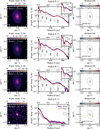 |
Fig. 1 From top to bottom: CI Tau’s ALMA Band 7, 6, 3, and VLA Ka band continuum emission. Left column: CLEAN images. Central column: Azimuthally averaged surface brightness radial profiles. Those obtained from the tclean images are in violet, purple is used for the best-fit frank profiles (a point-source component was subtracted from the 3.1 and 9.1 mm visibilities before fitting). Right column: residual images of the frank fit. Dotted ellipses mark the location of the dark rings in the CLEAN images. The synthesised CLEAN beam is shown as an ellipse in the bottom-left corner of each image and as a segment with full width half maximum equal to the beam minor axis in each radial profile subplot. |
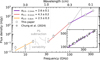 |
Fig. 2 CI Tau’s spectral flux density distribution. The grey dots display CI Tau’s photometry from this paper’s data and those of Rodmann et al. (2006). Photometry by Chung et al. (2024) is over-plotted with black dots in the insert. Full markers show the total flux density (i.e. before point-source subtraction) for the ALMA Band 3 and the VLA Q and Ka band data. The maximum and minimum integrated flux densities across different scans are displayed as smaller dots for the Ku and X band data to highlight their short timescale variability. |
3.2 Centimetre-wavelength emission
A number of physical processes were invoked to explain the centimetre-wavelength continuum emission in excess to thermal dust emission from circumstellar dust (Dulk 1985; Güdel 2002).
Free electrons interacting with circumstellar ionised gas produce bremsstrahlung (or free-free) thermal radiation. While in the case of emission from a homogeneous plasma, the spectral index is either α = 2.0, in the optically thick limit, or α = −0.1, in the optically thin one (Mezger et al. 1967), for an ionised, isothermal, spherically symmetric stellar wind, both for constant velocity and accelerated flows, emission scales with α = 0.6 (Wright & Barlow 1975; Panagia & Felli 1975; Olnon 1975). Instead, for a wider class of collimated ionised winds, the spectral index can be −0.1 ≤ α ≤ 2.0 (Reynolds 1986). While jets are typical of young Class 0/I sources (Anglada et al. 2018), free-free emission was attributed to collimated outflows also in a handful of more evolved systems, such as AB Aur (Rodríguez et al. 2014) and GM Aur (Macías et al. 2016), where elongated structures were detected in 3.0 cm images with 3 to 4σ significance. Optically thin free-free emission could well explain the slightly decreasing spectral index between the VLA Ku and (the visibility offset subtracted from the) Ka band data, and would also be consistent with the PS contribution to the ALMA Band 3 data. However, even in the optically thick regime, free-free emission is not fully consistent with the slope of the flux density distribution at wavelengths longer than 2.0 cm.
Other than circumstellar plasma, it was proposed that thermal free-free radiation could also originate from EUV-driven photoevaporative winds or the bound hot disc atmosphere close to the star heated up by X-ray irradiation (Pascucci et al. 2012; Owen et al. 2013). At wavelengths shorter than 10.0 cm, as is the case for our data, numerical models and radiative transfer calculations predict that free-free emission becomes optically thin, and its spectrum much flatter. As an example, for a 0.7 M⊙ star and at 3.0 cm, α ≲ 0.3 and 0.7 for the EUV and X-ray irradiation models (Owen et al. 2013), both too flat to explain by themselves the spectral indices measured in CI Tau between 2.0 and 5.0 cm.
Electrons whirling around the stellar magnetic field lines radiate non-thermal gyromagnetic emission. Depending on the particle velocity (relativistic or not) and electron energy distribution (thermal or power-law) gyromagnetic emission is characterised by different spectral indices (Dulk 1985; Güdel 2002). Radiation from highly relativistic electrons (synchrotron emission) is well described by a power-law electron distribution and a spectral index α = 2.5 in the optically thick regime and α ≤ −0.5 in the optically thin regime. In the case of mildly relativistic electrons (gyrosynchrotron radiation), both thermal and power-law electron distributions are possible scenarios. In the former case, α = 2.0 in the optically thick limit and α = −8.0 in the optically thin one, while in the latter, α = 2.5 in the optically thick limit and α ≤ −0.6 in the optically thin one (Dulk & Marsh 1982; Güdel 2002). Gyromagnetic radiation could broadly explain the excess radio emission between VLA Ku and C band in CI Tau, as well as the unresolved flux density offset in Ka band, provided that a sharp transition between optically thick and thin emission occurs at about 1.0 cm. However, its steep negative spectral index in the optically thin limit is not consistent with the unresolved flux density offset in ALMA Band 3 data.
It is well known that both free-free emission and gyromagnetic emission can be variable, but their characteristic timescales are expected to differ (Lommen et al. 2009; Ubach et al. 2012, 2017; Dzib et al. 2013, 2015; Liu et al. 2014; Coutens et al. 2019; Curone et al. 2023). While the former might change by 20 up to 40% over a few weeks to years, the latter can vary by a factor of two or more over a timescale of minutes to days (e.g. Ubach et al. 2012, 2017 and references therein). In Appendix D we show how CI Tau’s continuum luminosity changes by ≲30% over a timescale of a few minutes to weeks in the Ku band but is highly variable (by more than a factor of two) in the first 15 min of observations in the X band, as expected from gyromagnetic emission. No information on C band variability can be extracted due to the prohibitively low S/N of our data.
Therefore, we propose that optically thick gyrosynchrotron radiation most likely contributes to the excess emission (and connected variability) the most at wavelengths longer than 2.0 cm. Here, upon gyrosynchrotron emission transitioning from being optically thick to thin, optically thin free-free radiation becomes the dominant mechanism of non-dust emission down to wavelengths as short as 3.1 mm. Monitoring CI Tau over weeks to months with deeper follow-up multi-wavelength (between 9.1 mm to 6.0 cm) and multi-epoch observations is necessary to conclusively assess the origin of centimetre-wavelength continuum emission in this source.
3.3 Spectral index radial profiles
Our high-resolution observations can be used to study how the spectral index changes as a function of the disc radius. To do so, we first subtracted the point-source visibility offset measured in Appendix C.1 to the real part of the ALMA Band 3 (for both XX and YY polarisations) and the VLA Ka band (only for the RR and LL polarisations) visibilities. Then we imaged each dataset using two different synthesised beams: (i) we reconstructed the ALMA and VLA Ka band observations using a circular beam with ![Mathematical equation: $\[0^{\prime\prime}_\cdot195\]$](/articles/aa/full_html/2025/10/aa52986-24/aa52986-24-eq8.png) radius. This conservative choice allowed us to recover the VLA Ka band outer-disc emission displayed in Figure 1 with S/N > 3; (ii) we also imaged the ALMA data with a smaller,
radius. This conservative choice allowed us to recover the VLA Ka band outer-disc emission displayed in Figure 1 with S/N > 3; (ii) we also imaged the ALMA data with a smaller, ![Mathematical equation: $\[0^{\prime\prime}_\cdot058 \times 0^{\prime\prime}_\cdot087\]$](/articles/aa/full_html/2025/10/aa52986-24/aa52986-24-eq9.png) , PA = −33.20 deg beam. This is the best trade off between angular resolution and sensitivity for Band 7 data (those with shortest maximum baseline). In this case, we chose not to circularise the beam to keep the maximum angular resolution compatible with our data.
, PA = −33.20 deg beam. This is the best trade off between angular resolution and sensitivity for Band 7 data (those with shortest maximum baseline). In this case, we chose not to circularise the beam to keep the maximum angular resolution compatible with our data.
To minimise any uncertainty due to convolution in the image plane, we first CLEANed each dataset adopting different uvtaper parameters to reach a similar beam shape (i.e. beam axes within ≤1.5 mas and position angles within ≤0.02 deg) to our target ones. Only then, these images were smoothed, using the imsmooth task, to our target beam sizes. The optimal tapering parameters were found by trial and error, simulating the CASA PSF reconstruction routine. For each target beam, we explored different combinations of the robust and uvtaper parameters, but no notable differences were found. Finally, these smoothed intensity maps were deprojected as explained in Section 2.3 and their azimuthally averaged radial profiles were used to compute the spectral index radius by radius as
![Mathematical equation: $\[\alpha_{\nu_1-\nu_2}=\frac{\log I_{\nu_1}-\log I_{\nu_2}}{\log \nu_1-\log \nu_2},\]$](/articles/aa/full_html/2025/10/aa52986-24/aa52986-24-eq10.png) (1)
(1)
where Iν is the azimuthally averaged surface brightness profile at frequency ν. We preferred this method over the alternative strategy of computing 2D spectral index maps from CLEAN images at different wavelengths using the immath task. In fact, when deprojected and azimuthally averaged, such maps generally provide much noisier spectral index radial profiles.
CI Tau’s spectral index profiles measured between pairs of progressively longer wavelengths are plotted as solid lines in Figure 3. The shaded regions, instead, display their uncertainty, obtained propagating the quadrature sum of the error of the mean of each surface brightness radial profile and their absolute flux calibration uncertainty. The hatched regions mark the locations where S/N ≤ 5 (left and central panel) and S/N ≤ 3 (right panel) for at least one of the emission profiles. These profiles are plotted as dashed lines in the background.
The spectral indices between ALMA Band 7 and 6, αB7–B6, and between ALMA Band 6 and 3, αB6–B3, data increase towards the outer disc, suggesting that emission is optically thinner at large radii or tracing radial variations of the dust opacity owing most likely to (a larger fraction of) smaller grains further away from the central star. At the position of the bright rings, marked by the vertical dashed-dotted lines and labelled as in Figure 1, the spectral index radial profiles reach local minima, as expected in the case of more optically thick emission or the presence of (a larger fraction of) larger grains. This trend is more easily seen for αB7–B6 than αB6–B3, whose profile shows much shallower modulations. This difference can be explained by: (i) the different ring-to-gap contrast in the surface brightness radial profiles at different wavelengths. Indeed, while this contrast increases between ALMA Band 7 and 6 observations, it is very similar for ALMA Band 6 and 3 data (see the grey dashed lines in Figure 3). This trend can be interpreted as a consequence of emission being optically thin(ner) at 1.3 and 3.1 mm. In this regime, the less substructured spectral index radial profile between ALMA Band 6 and 3 data suggests that only small modulations of the grain size radial profile at the location of gaps and rings might be expected; (ii) the different gap and ring centres in Band 6 and 3 data (e.g. the outer disc gap in the central panel of Figure 3).
As already discussed in Section 3.1, compared with αB7–B6 and αB6–B3, the spectral index between ALMA Band 3 and VLA Ka band data, αB3–Ka, is larger (notice the different scale in the right panel of Figure 3), suggesting that emission is optically thin at these wavelengths. Also αB3–Ka increases towards the outer disc, albeit only until the VLA Ka band brightness profile flatten out due to its lower S/N. No modulations due to substructures in the emission profiles can be seen.
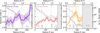 |
Fig. 3 Spectral index radial profiles (solid lines) and their 1σ uncertainty (shaded areas). The hatched regions mark those locations where S/N ≤ 5 (left and central panel) and 3 (right panel), for at least one of the emission profiles. The dashed grey lines in each panel display the surface brightness radial profiles combined to determine the spectral index. |
4 Analysis method
4.1 Model
The spectral dependence of dust emission can inform us about dust properties such as their temperature (Tdust), density (Σdust), size, composition, and morphology. To try and constrain (at least some of) these quantities, we fitted CI Tau’s surface brightness profiles between 0.9 and 9.1 mm, radius by radius, adopting a physical model that takes into account the effects of optical depth and dust scattering (e.g. Carrasco-González et al. 2019; Macías et al. 2021; Sierra et al. 2021; Guidi et al. 2022). According to this model, in the case of an azimuthally symmetric, vertically isothermal, and razor-thin disc, dust thermal emission from the disc mid-plane can be computed as (Rybicki & Lightman 1986; Miyake & Nakagawa 1993; Carrasco-González et al. 2019)
![Mathematical equation: $\[S_\nu\left(\tau_\nu, \mu\right)=B_\nu\left(T_{\text {dust }}\right)\left[1-\exp \left(-\tau_\nu / \mu\right)+\omega_\nu F\left(\tau_\nu, \omega_\nu, \mu\right)\right],\]$](/articles/aa/full_html/2025/10/aa52986-24/aa52986-24-eq11.png) (2)
(2)
where Bν(Tdust) is the black body emission at temperature Tdust and frequency ν, τν = Σdusχν is the disc optical depth, ![Mathematical equation: $\[\chi_{\nu}=\kappa_{\nu}^{\mathrm{abs}}+\kappa_{\nu}^{\mathrm{sca}}\]$](/articles/aa/full_html/2025/10/aa52986-24/aa52986-24-eq12.png) is the total dust opacity,
is the total dust opacity, ![Mathematical equation: $\[\kappa_{\nu}^{\mathrm{abs}}\]$](/articles/aa/full_html/2025/10/aa52986-24/aa52986-24-eq13.png) and
and ![Mathematical equation: $\[\kappa_{\nu}^{\mathrm{sca}}\]$](/articles/aa/full_html/2025/10/aa52986-24/aa52986-24-eq14.png) are the absorption and scattering opacities, μ = cos i is the disc inclination (that we fixed to the best-fit value of Clarke et al. 2018),
are the absorption and scattering opacities, μ = cos i is the disc inclination (that we fixed to the best-fit value of Clarke et al. 2018), ![Mathematical equation: $\[\omega_{\nu}=\kappa_{\nu}^{\mathrm{sca}} / \chi_{\nu}\]$](/articles/aa/full_html/2025/10/aa52986-24/aa52986-24-eq15.png) is the single-scattering albedo, and
is the single-scattering albedo, and
![Mathematical equation: $\[\begin{aligned}F\left(\tau_\nu, \omega_\nu, \mu\right)= & \frac{1}{\exp \left(-\sqrt{3} \epsilon_\nu \tau_\nu\right)\left(\epsilon_\nu-1\right)-\left(\epsilon_\nu+1\right)} \\& \times\left[\frac{1-\exp \left(-\left(\sqrt{3} \epsilon_\nu+1 / \mu\right) \tau_\nu\right)}{\sqrt{3} \epsilon_\nu \mu+1}\right. \\& \left.+\frac{\exp \left(-\tau_\nu / \mu\right)-\exp \left(-\sqrt{3} \epsilon_\nu \tau_\nu\right)}{\sqrt{3} \epsilon_\nu \mu-1}\right],\end{aligned}\]$](/articles/aa/full_html/2025/10/aa52986-24/aa52986-24-eq16.png) (3)
(3)
where ![Mathematical equation: $\[\epsilon_{\nu}=\sqrt{1-\omega_{\nu}}\]$](/articles/aa/full_html/2025/10/aa52986-24/aa52986-24-eq17.png) . In the simplest possible assumption that the absorption and scattering opacities scale with frequency as a single-power law (i.e.
. In the simplest possible assumption that the absorption and scattering opacities scale with frequency as a single-power law (i.e. ![Mathematical equation: $\[\kappa_{\nu}^{\text {abs}}=\kappa_{\nu_{0}}^{\text {abs}} \nu^{\beta^{\text {abs}}}\]$](/articles/aa/full_html/2025/10/aa52986-24/aa52986-24-eq18.png) and
and ![Mathematical equation: $\[\kappa_{\nu}^{\text {sca }}=\kappa_{\nu_{0}}^{\text {sca}} \nu^{\beta^{\text {sca}}}\]$](/articles/aa/full_html/2025/10/aa52986-24/aa52986-24-eq19.png) , where
, where ![Mathematical equation: $\[\kappa_{\nu_{0}}^{\text {abs}}\]$](/articles/aa/full_html/2025/10/aa52986-24/aa52986-24-eq20.png) and
and ![Mathematical equation: $\[\kappa_{\nu_{0}}^{\text {sca}}\]$](/articles/aa/full_html/2025/10/aa52986-24/aa52986-24-eq21.png) are normalisation coefficients), Equation 2 depends on six free parameters (Tdust,
are normalisation coefficients), Equation 2 depends on six free parameters (Tdust, ![Mathematical equation: $\[\Sigma_{\text {dust}}, \kappa_{\nu_{0}}^{\text {abs}}, \beta^{\text {abs}}, \kappa_{\nu_{0}}^{\text {sca}}\]$](/articles/aa/full_html/2025/10/aa52986-24/aa52986-24-eq22.png) , and βsca). Thus, at least six datasets at different frequencies would be required to observationally constrain such parameters. Since this is currently not feasible in the case of CI Tau, where only four high angular resolution and sensitivity datasets are available, we adopted a different strategy (e.g. Carrasco-González et al. 2019; Macías et al. 2021). Instead of fitting for the absorption and scattering opacities self-consistently, we assumed a bulk dust composition and computed its optical properties, hence
, and βsca). Thus, at least six datasets at different frequencies would be required to observationally constrain such parameters. Since this is currently not feasible in the case of CI Tau, where only four high angular resolution and sensitivity datasets are available, we adopted a different strategy (e.g. Carrasco-González et al. 2019; Macías et al. 2021). Instead of fitting for the absorption and scattering opacities self-consistently, we assumed a bulk dust composition and computed its optical properties, hence ![Mathematical equation: $\[\kappa_{\nu}^{\text {abs}}\]$](/articles/aa/full_html/2025/10/aa52986-24/aa52986-24-eq23.png) and
and ![Mathematical equation: $\[\kappa_{\nu}^{\text {sca}}\]$](/articles/aa/full_html/2025/10/aa52986-24/aa52986-24-eq24.png) , as a function of the maximum grain size (amax) and for a grain size power law distribution (n(a)da ∝ a−qda, where n(a) is the dust number density in a small size interval da). Thus the number of free parameters was reduced from six to four (Tdust, Σdust, amax, and q). Adopting a set of dust bulk properties also allowed us to correct for the assumption of isotropic scattering in Equation (2), compute the forward-scattering coefficient (gν, Henyey & Greenstein 1941), and rescale the scattering opacity as
, as a function of the maximum grain size (amax) and for a grain size power law distribution (n(a)da ∝ a−qda, where n(a) is the dust number density in a small size interval da). Thus the number of free parameters was reduced from six to four (Tdust, Σdust, amax, and q). Adopting a set of dust bulk properties also allowed us to correct for the assumption of isotropic scattering in Equation (2), compute the forward-scattering coefficient (gν, Henyey & Greenstein 1941), and rescale the scattering opacity as ![Mathematical equation: $\[\kappa_{\nu}^{\text {sca,eff}}=\left(1-g_{\nu}\right) \kappa_{\nu}^{\text {sca}}\]$](/articles/aa/full_html/2025/10/aa52986-24/aa52986-24-eq25.png) .
.
In this scenario, the composition, porosity, and mixing rules adopted to determine the dust optical properties are essential. Indeed, it is well known that different opacities can lead to significantly different estimates of the temperature, density, and size of dust (see e.g. Banzatti et al. 2011; Ohashi et al. 2023; Sierra et al. 2025). Most of the previously published analyses of high angular resolution multi-frequency continuum observations similar to ours considered grains to be compact and spherical and adopted the default dust mixture proposed by Birnstiel et al. (2018) as a reference for the DSHARP survey (Andrews et al. 2018). In this paper, instead, we chose a different fiducial composition: we considered dust to be made of 60% water ice (Warren & Brandt 2008), 30% amorphous carbon (Zubko et al. 1996, ACH2 sample), and 10% astronomical silicates (Draine 2003) by volume. This mixture differs from that proposed by Ricci et al. (2010b) only for their higher porosity (30%)4. For this reason, we refer to our fiducial opacities as ‘Ricci (compact)’. Although, at the current stage, our choice might seem arbitrary, in Section 6 we extensively discuss how our results depend on the adopted bulk dust properties, exploring different compositions and porosity filling factors, and providing a justification for our fiducial opacities. Furthermore, in recent years indirect evidence in favour of mixtures rich in amorphous carbon, such as the ‘Ricci (compact)’ one, came from demographic disc studies in nearby star-formation regions such as those modelling the size-luminosity correlation (Rosotti et al. 2019a; Zormpas et al. 2022) and the spectral index distribution (Stadler et al. 2022; Delussu et al. 2024). We used the dsharp_opac package (Birnstiel et al. 2018) to determine the dielectric constants of our fiducial mixture5 from the refractive indices of the aforementioned materials adopting the Bruggeman rule (Bruggeman 1935, see Appendix A of Zhang et al. 2023 for a justification), and its optical properties using Mie theory for spherical grains (Bohren & Huffman 1998).
4.2 Fitting procedure
We adopted a Bayesian approach and used emcee (Foreman-Mackey et al. 2013, 2019), a pure-Python implementation of the affine-invariant Markov chain Monte Carlo (MCMC) ensemble sampler of Goodman & Weare (2010) to estimate the posterior distribution of the model parameters at each radius. Our log-likelihood function reads as
![Mathematical equation: $\[\ln p\left(I_\nu {\mid} \boldsymbol{\theta}\right)=-\frac{1}{2} \sum_\nu\left[\left(\frac{I_\nu-S_\nu}{\sigma_{\nu, \mathrm{tot}}}\right)^2+\ln (2 \pi \sigma_{\nu, \mathrm{tot}}^2)\right],\]$](/articles/aa/full_html/2025/10/aa52986-24/aa52986-24-eq26.png) (4)
(4)
where θ = {Tdust, Σdust, amax, q} is the parameter vector, Iν is the azimuthally averaged dust surface brightness radial profile at frequency ν and radius R (from the observations), Sν is the model surface brightness radial profile (from Equation (2)), and
![Mathematical equation: $\[\sigma_{\nu, \mathrm{tot}}^2=\sigma_\nu^2+\left(\delta I_\nu\right)^2,\]$](/articles/aa/full_html/2025/10/aa52986-24/aa52986-24-eq27.png) (5)
(5)
where σν is the uncertainty of the azimuthally averaged brightness profile at frequency ν and radius R, while δIν indicates the systematic flux calibration uncertainty. Following the recommendations of the ALMA Technical Handbook6 and the Guide to Observing with the VLA7, we assumed δ = 10% for ALMA Band 7, 6, and the VLA Ka band observations, and δ = 5% for the ALMA Band 3 data.
We benchmarked our fitting procedure against the results of Macías et al. (2021) in TW Hya, using their publicly available self-calibrated high angular resolution multi-frequency continuum observations, the same dust composition, model priors, and parameter ranges. Our results are in excellent agreement with their marginalised posterior distributions for each of the fitting parameters, both in the case of a fixed ISM-like particle size distribution and when q is allowed to change.
To assess convergence we estimated the integrated autocorrelation time, τe, using the method of Sokal (1997). Since τe often increases with the number of MCMC steps, we first adopted a restrictive convergence criterion: we considered our chains to be converged if they are longer than 100 times the maximum estimated integrated autocorrelation time for each parameter, max(τe), and if this quantity changes by less than 1% over the last 103 steps. To speed-up convergence, we first fitted Equation (2) to our spectral flux density distribution, using the Trust Region Reflective minimisation algorithm for bound problems implemented in scipy.optimize.curve_fit and initialised our walkers in a 4D sphere in the parameter space around these best-fit values. Moreover, instead of the default ‘stretch move’ of Goodman & Weare (2010), we adopted a weighted mixture of the ‘differential evolution proposal’ (Ter Braak 2006) and the ‘snooker proposal’ (Ter Braak & Vrugt 2008) moves, randomly selected with 80% and 20% probability, achieving a twice as fast convergence.
We tested this convergence criterion using TW Hya data for R = 25, 30, and 45 au (because at these locations our posterior distributions can be compared with the corner-plots published by Macías et al. 2021). When exploring the parameter space with 102 walkers, this criterion requires chains longer than 1.6 × 10⁴ steps and gives max(τe) ≤ 1.4 × 10². Since this is impractically long to run for hundreds of fits, for the rest of the paper we used 102 walkers and 103 steps, ≈7.5 times longer than max(τe), and sampled the posterior distribution function discarding, on average, the initial 2 to 4 × 10² ‘burn-in’ steps (corresponding to five times the maximum estimated integrated autocorrelation time of these shorter chains). This choice gives results in remarkable agreement with those obtained with our more restrictive convergence criterion and the corner plots of Macías et al. (2021). Our acceptance fractions were, on average, ≤0.3.
4.3 Two-step methodology
The main issue to deal with when fitting Equation (2) to the data is the lower S/N of the VLA Ka band observations compared to the ALMA ones. Fitting all our high-resolution data together (i.e. data at the three ALMA bands and the VLA Ka band) requires either (i) adopting a large-enough beam to recover the outer disc emission in the VLA Ka band data, thus giving up the possibility of constraining the properties of dust on the scale of the gaps and rings in the system, or (ii) considering only the higher quality ALMA data. However, this generally leads to a bimodal dust size distribution and generally poorer constraints on dust properties (as was discussed by e.g. Macías et al. 2021; Sierra et al. 2021; Ueda et al. 2022). To take the best out of these two scenarios (tight constraints on dust properties from the VLA data, on the scale of gaps and rings in the ALMA images) we adopted a different method.
We first considered the low angular resolution surface brightness radial profiles (i.e. those reconstructed with a ![Mathematical equation: $\[0^{\prime\prime}_\cdot195\]$](/articles/aa/full_html/2025/10/aa52986-24/aa52986-24-eq28.png) circular beam) and fitted Equation (2) to the spectral flux density distribution from 0.9 mm to 9.1 mm in each radial bin, Iν(Ri + ΔR), independently (i.e. averaging the emission intensity in each pixel of width ΔR = 19.5 mas ≈ 3.1 au, for a progressively larger radius Ri+1 = Ri + ΔR). We adopted uninformative priors for all the parameters, except the temperature. In this case, following Macías et al. (2021), our prior is based on the expected temperature profile of a passively irradiated disc as summarised in Appendix E. The other parameters were free to vary in the following ranges: −3 ≤ log(Σdust/g cm−2) ≤ 3, −3 ≤ log(amax/cm) ≤ 3, and 1 ≤ q ≤ 4. The posterior distributions of this ‘low resolution’ fit were then used as priors for a ‘high resolution’ fit to the ALMA-only surface brightness radial profiles reconstructed with a
circular beam) and fitted Equation (2) to the spectral flux density distribution from 0.9 mm to 9.1 mm in each radial bin, Iν(Ri + ΔR), independently (i.e. averaging the emission intensity in each pixel of width ΔR = 19.5 mas ≈ 3.1 au, for a progressively larger radius Ri+1 = Ri + ΔR). We adopted uninformative priors for all the parameters, except the temperature. In this case, following Macías et al. (2021), our prior is based on the expected temperature profile of a passively irradiated disc as summarised in Appendix E. The other parameters were free to vary in the following ranges: −3 ≤ log(Σdust/g cm−2) ≤ 3, −3 ≤ log(amax/cm) ≤ 3, and 1 ≤ q ≤ 4. The posterior distributions of this ‘low resolution’ fit were then used as priors for a ‘high resolution’ fit to the ALMA-only surface brightness radial profiles reconstructed with a ![Mathematical equation: $\[0^{\prime\prime}_\cdot058 \times 0^{\prime\prime}_\cdot087\]$](/articles/aa/full_html/2025/10/aa52986-24/aa52986-24-eq29.png) PA = −33.20 deg beam. We fitted Equation (2) to the spectral flux density distribution from 0.9 mm to 3.1 mm in each radial bin (with ΔR = 11.6 mas ≈ 1.9 au) independently.
PA = −33.20 deg beam. We fitted Equation (2) to the spectral flux density distribution from 0.9 mm to 3.1 mm in each radial bin (with ΔR = 11.6 mas ≈ 1.9 au) independently.
To do so, for each selected radius in the high resolution profiles, we first identified the closest (‘reference’) radial bin in the low resolution profiles. Then, we estimated non-parametrically the probability density function of the marginalised posterior distribution of each parameter fitting the posterior samples using the scipy.stats.gaussian_kde function (Virtanen et al. 2020). We only fitted the (>7 × 10³) samples left after discarding the first 5 × max(τe) ‘burn-in’ steps and thinning the sample set by a factor of 0.5 × max(τe) ≈ 15. Finally, for every MCMC step and fitting parameter, θi, we determined the marginalised prior through a one-dimensional piecewise linear interpolation to the KDE marginalised posterior probability density function, pKDE(θi|Iν). Our final prior reads as
![Mathematical equation: $\[\begin{aligned}& \ln~ p(\boldsymbol{\theta})=\ln~ p\left(T_{\text {dust }}\right) \\& \quad+\ln~ p_{\mathrm{KDE}}\left(\Sigma_{\text {dust}} {\mid} I_\nu\right)+\ln~ p_{\mathrm{KDE}}\left(a_{\max} {\mid} I_\nu\right)+\ln~ p_{\mathrm{KDE}}\left(q {\mid} I_\nu\right),\end{aligned}\]$](/articles/aa/full_html/2025/10/aa52986-24/aa52986-24-eq30.png) (6)
(6)
where p(Tdust) is the temperature prior from Appendix E, while Iν indicates the ![Mathematical equation: $\[0^{\prime\prime}_\cdot195\]$](/articles/aa/full_html/2025/10/aa52986-24/aa52986-24-eq31.png) resolution ALMA and VLA Ka band surface brightness profiles at the reference radius. We initialised our walkers around the median of the posterior distribution of the low resolution fit in the same reference radial bin to achieve a faster convergence. While writing this paper, we became aware that a similar double-fit analysis method had been independently developed by Viscardi et al. (2025), who also benchmarked it against collisional growth and dust transport DustPy (Stammler & Birnstiel 2022) models. The analysis of Viscardi et al. (2025) lends further support to the validity of our results and we refer to their paper for further insights and validation.
resolution ALMA and VLA Ka band surface brightness profiles at the reference radius. We initialised our walkers around the median of the posterior distribution of the low resolution fit in the same reference radial bin to achieve a faster convergence. While writing this paper, we became aware that a similar double-fit analysis method had been independently developed by Viscardi et al. (2025), who also benchmarked it against collisional growth and dust transport DustPy (Stammler & Birnstiel 2022) models. The analysis of Viscardi et al. (2025) lends further support to the validity of our results and we refer to their paper for further insights and validation.
4.4 Cross-composition comparison
We explored the dependence of our results on dust composition by fitting CI Tau’s low-resolution (![Mathematical equation: $\[0^{\prime\prime}_\cdot195\]$](/articles/aa/full_html/2025/10/aa52986-24/aa52986-24-eq32.png) circular beam) radial profiles with a range of different optical properties and comparing their posterior distributions.
circular beam) radial profiles with a range of different optical properties and comparing their posterior distributions.
In Bayesian statistics, two models, m1 and m2, can be compared computing the so-called Bayes factor. This is the ratio of the marginalised likelihoods, p(Iν|m1) p(m1) and p(Iν|m2) p(m2), where
![Mathematical equation: $\[p\left(I_\nu {\mid} m_i\right)=\int p\left(I_\nu {\mid} \boldsymbol{\theta}, m_i\right) p\left(\boldsymbol{\theta} {\mid} m_i\right) d \boldsymbol{\theta},\]$](/articles/aa/full_html/2025/10/aa52986-24/aa52986-24-eq33.png) (7)
(7)
for i = 1, 2, is the posterior normalisation or model evidence. Unfortunately, emcee does not provide such a marginalised likelihood and estimating it from the posterior samples is non-trivial (e.g. Hou et al. 2014). For this reason, we adopted the χ2 test as a measure of the goodness of our fit and postponed a more thorough and fully Bayesian analysis to a future paper. Since models with the same number of free parameters are compared, we expect this metric to be a sufficiently robust indicator of the quality of our models.
For each adopted composition, we provide two estimates of the reduced χ2, based on the surface brightness and spectral index radial profiles. As for the surface brightness, first, for each radius, we used our MCMC samples to determine the posterior distributions of the model intensity, Sν, and estimated the reduced χ2 posterior distribution as
![Mathematical equation: $\[\chi_{\mathrm{SB}}^2=\frac{1}{4} \sum_\nu\left(\frac{I_\nu-S_\nu}{\sigma_{\nu, \mathrm{tot}}}\right)^2,\]$](/articles/aa/full_html/2025/10/aa52986-24/aa52986-24-eq34.png) (8)
(8)
where the sum runs over all the four frequencies our data were taken at, Iν and σν,tot have the same meaning as in Section 4.2, while Sν is a model realisation from each sample of the parameter posteriors. We then determined a disc-averaged χ2 posterior distribution concatenating the last n samples of the ![Mathematical equation: $\[\chi_{\mathrm{SB}}^{2}\]$](/articles/aa/full_html/2025/10/aa52986-24/aa52986-24-eq35.png) posterior distribution for each radius smaller than some maximum disc size Rout. Since the number of available
posterior distribution for each radius smaller than some maximum disc size Rout. Since the number of available ![Mathematical equation: $\[\chi_{\mathrm{SB}}^{2}\]$](/articles/aa/full_html/2025/10/aa52986-24/aa52986-24-eq36.png) samples is radiusdependent, we chose n as the minimum sample length among all radii smaller than Rout. As for Rout, instead, we adopted three different definitions: Rout ≈ 200 au, the maximum radius we could fit our data for (at larger radii the low surface brightness S/N leads to unphysical results), Rout = 151 and 82 au, the disc locations where the S/N of our VLA Ka band and brightness profile drops below 3 and 5, respectively.
samples is radiusdependent, we chose n as the minimum sample length among all radii smaller than Rout. As for Rout, instead, we adopted three different definitions: Rout ≈ 200 au, the maximum radius we could fit our data for (at larger radii the low surface brightness S/N leads to unphysical results), Rout = 151 and 82 au, the disc locations where the S/N of our VLA Ka band and brightness profile drops below 3 and 5, respectively.
We adopted a similar strategy for the χ2 posterior distribution estimated from the spectral index radial profiles. In this case, at a given radius, the reduced χ2 reads
![Mathematical equation: $\[\chi_{\mathrm{SI}}^2=\frac{1}{3} \sum_i\left(\frac{\alpha_{i, \mathrm{obs}}-\alpha_{i, \mathrm{mod}}}{\sigma_{\alpha_i, \mathrm{tot}}}\right)^2,\]$](/articles/aa/full_html/2025/10/aa52986-24/aa52986-24-eq37.png) (9)
(9)
where the subscripts ‘obs’ and ‘mod’ stand for the observed spectral index and a model realisation from each sample of the parameter posteriors, while the index i runs over pairs of subsequent frequencies (i.e. αB7–B6, αB6–B3, and αB3–Ka). σαi,tot, instead, is the observed spectral index uncertainty, estimated propagating the errors on each surface brightness radial profile, that also include the absolute flux calibration uncertainty.
5 Results
5.1 Best-fit radial profiles, fiducial case
Our results are shown in Figure 4, while we defer to Appendix F a discussion on the goodness of our fit. The blue solid lines and shaded regions display the best-fit profiles and their 1σ uncertainty (defined as the median and the area between the 16th and 84th percentile of the marginalised posterior distribution of each parameter). For the sake of comparison, the median and 1σ spread are plotted also for the low resolution fit as dotted lines and paler shaded areas of the same colour. As can be seen, the low resolution fit is able to constrain remarkably well the four fitting parameters. However, their radial profiles are only sensitive to global variations and low-amplitude modulations at the location of the outer ring (the only substructure that is marginally resolved with an angular resolution of ![Mathematical equation: $\[0^{\prime\prime}_\cdot195\]$](/articles/aa/full_html/2025/10/aa52986-24/aa52986-24-eq38.png) ). Thanks to their smaller beam, the high resolution best-fit radial profiles, instead, show clear modulations at the position of all the rings (see e.g. the ALMA Band 6 surface brightness radial profile over-plotted as a grey dashed line, where the ring positions are indicated by the vertical dashed-dotted lines and labelled as in Figure 1).
). Thanks to their smaller beam, the high resolution best-fit radial profiles, instead, show clear modulations at the position of all the rings (see e.g. the ALMA Band 6 surface brightness radial profile over-plotted as a grey dashed line, where the ring positions are indicated by the vertical dashed-dotted lines and labelled as in Figure 1).
Starting from the top left panel, the best-fit temperature profile reflects our passively irradiated disc prior and shows no clear substructures. Instead, the dust surface density radial profile locally peaks at the position of the bright rings. In particular, the 27 au, 60 au, and 152 au rings are 9%, 14%, and 37% denser than their preceding gaps. Similar features were already observed in some rings, for example, in HL Tau (Carrasco-González et al. 2019; Guerra-Alvarado et al. 2024), TW Hya (Macías et al. 2021), HD 163296 (Guidi et al. 2022), and the MAPS discs (Sierra et al. 2021). We do not detect the sharp dust surface density outer edge predicted by Birnstiel & Andrews (2014) to be a signpost of radial drift. However, this is likely due the low S/N of our data in the outer disc (R ≳ 200 au). Our best-fit maximum grain size radial profile is flat within the uncertainties and amax ≈ 7.4 × 10⁻² cm. Moreover, it shows no clear substructures, with the exception of a marginal (11%) increase at the position of the outer gap. However, this modulation lies well within the uncertainties and is not statistically significant. Indeed, we do not consider it to be physical, but an artefact of the fit, owing to the low S/N ≳ 3 of the VLA Ka band radial profile at this location (see the black and grey arrows at the bottom-left corner of each panel that mark the detection significance of the VLA Ka band surface brightness radial profile). Deeper data are needed to confirm this hypothesis. The absence of substructures in the maximum grain size radial profile is also a common feature to many of the sources targeted at multiple wavelengths and high angular resolution by ALMA (see e.g. Jiang et al. 2024). Finally, our density distribution power-law index radial profile increases from q ≈ 3.0 in the inner disc to q > 3.5 in the outer disc, with local troughs at the position of the bright rings, similarly to the case TW Hya (Macías et al. 2021).
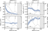 |
Fig. 4 Dust temperature, density, maximum size, and density distribution power-law index posterior distributions for our fiducial ‘Ricci (compact)’ composition. The blue solid lines and shaded regions display the median and 1σ uncertainty of each parameter. For comparison, the dotted lines show the results of the low resolution fit. The hatched areas mark the disc region within the synthesised beam minor axis ( |
![Mathematical equation: $\[0^{\prime\prime}_\cdot058\]$](/articles/aa/full_html/2025/10/aa52986-24/aa52986-24-eq39.png)
![Mathematical equation: $\[0^{\prime\prime}_\cdot058\]$](/articles/aa/full_html/2025/10/aa52986-24/aa52986-24-eq40.png)
5.2 Optical properties, fiducial case
Figure 5 shows the best-fit radial profiles and the 1σ uncertainties of the dust optical properties, computed from the posterior distributions discussed in Section 4.1. The solid lines display the ALMA-only high resolution fit results, while the dotted ones are used for the combined ALMA and VLA Ka band low resolution fit, colour-coded by the reference wavelength of our datasets.
First and foremost, the upper-left panel shows that the optical depth is moderate to low between 0.9 and 9.1 mm (τν ≲ 1), suggesting that CI Tau’s continuum emission is (marginally) optically thin at all the radii at these wavelengths. Our low and high resolution fits display similar trends, with τν decreasing towards the outer disc and longer wavelengths. Such a decrease becomes even sharper when the disc radius or the observational wavelength increases, suggesting that dust emission is progressively optically thinner in the outer disc and at longer wavelengths. The results of the high resolution fit also show that τν locally increases at the position of the bright rings. These profiles closely match the spectral index behaviour discussed in Section 3.3.
The upper-right panel displays the absorption optical depth, ![Mathematical equation: $\[\tau_{\nu}^{\text {abs}}=\Sigma_{\text {dust}} \kappa_{\nu}^{\text {abs}}\]$](/articles/aa/full_html/2025/10/aa52986-24/aa52986-24-eq41.png) . On top of the results from our high and low resolution fits, the black dotted lines show the absorption optical depth profiles inferred from each dataset separately in the optically thin limit (see e.g. Huang et al. 2018b; Dullemond et al. 2018) as
. On top of the results from our high and low resolution fits, the black dotted lines show the absorption optical depth profiles inferred from each dataset separately in the optically thin limit (see e.g. Huang et al. 2018b; Dullemond et al. 2018) as
![Mathematical equation: $\[\frac{I_\nu}{B_\nu}=1-\exp \left(-\frac{\tau_\nu^{\mathrm{abs}}}{\cos~ i}\right) \rightarrow \tau_\nu^{\mathrm{abs}}=-\cos~ i ~\ln \left(1-\frac{I_\nu}{B_\nu}\right),\]$](/articles/aa/full_html/2025/10/aa52986-24/aa52986-24-eq42.png) (10)
(10)
where the dust temperature was estimated as in Equation (E.1) fixing ϕ = 0.02 and L⋆ = 1.04 L⊙. Unsurprisingly, since continuum emission is (marginally) optically thin, the absorption optical depth profiles inferred from Equation (10) are in excellent agreement (less than a factor of two off) with those estimated from the posterior distribution of our multi-frequency analysis. By direct comparison with the profiles plotted in the upper-left panel, it can be seen that absorption contributes by about 50% (ALMA Band 3) to 60% (ALMA Band 7,6, and VLA Ka band) to the total dust opacity. This is a consequence of our fiducial dust composition, whose single-scattering albedo, plotted in the bottom-left panel, is by construction ≲ 0.5 at all the wavelengths.
CI Tau’s low optical depth stands out when compared with that of the other sources targeted in previous multi-frequency high resolution studies. In particular, only GM Aur (Sierra et al. 2021) shows a comparably low optical depth at (sub-)millimetre wavelengths. All the other sources, instead, are optically thick down to a few millimetres (ALMA Band 3 or 4) either in the inner 20 to 50 au, such as TW Hya (Macías et al. 2021), HD 163296 (Sierra et al. 2021; Guidi et al. 2022), AS 209 and MWC 480 (Sierra et al. 2021), or at all the radii, such as HL Tau (Carrasco-González et al. 2019; Zhang et al. 2023) and IM Lup (Sierra et al. 2021). Although this comparison is most likely affected by the different spectral coverage of these datasets and the assumptions on composition adopted in these works, we stress that our conclusion that CI Tau is optically thin at (sub-)millimetre to centimetre wavelengths is robust: with the exception of highly porous material, all the different compositions tested in Section 6 consistently recover optical depths τν ≲ 1 across all the modelled datasets and the same ![Mathematical equation: $\[\tau_{\nu}^{\text {abs}}\]$](/articles/aa/full_html/2025/10/aa52986-24/aa52986-24-eq43.png) (see Appendix G). Moreover, at least in those discs, HL Tau (Carrasco-González et al. 2019; Zhang et al. 2023) and HD 163296 (Guidi et al. 2022), where high-resolution centimetre-wavelength data are available, the much shallower spectral index between 2.1/3.0 mm and 8.0/9.1 mm than in CI Tau indicates a genuinely higher optical depth (unless the dust composition differs substantially among these source).
(see Appendix G). Moreover, at least in those discs, HL Tau (Carrasco-González et al. 2019; Zhang et al. 2023) and HD 163296 (Guidi et al. 2022), where high-resolution centimetre-wavelength data are available, the much shallower spectral index between 2.1/3.0 mm and 8.0/9.1 mm than in CI Tau indicates a genuinely higher optical depth (unless the dust composition differs substantially among these source).
At ALMA wavelengths the (absorption) optical depth trends displayed in Figure 5 are primarily determined by the shape of the dust surface density. Indeed, as can be noticed in the lower right panel, the total dust opacity hardly changes with radius for λ ≤ 3.1 mm. This is due to the maximum grain size radial profile being flat (see Figure 4) and the weak dependence of χν on q (less than a factor of three at most radii). At 9.1 mm, instead, since our inferred maximum grain size falls around the Mie interference at amax ≈ λ/2π, the total dust opacity rapidly decreases with q (a factor of ten for 3.0 ≤ q ≤ 4.0) and the opacity radial variations affect the shape of the optical depth radial profile the most. These results highlight the importance of the Mie resonance in determining the optical depth as a function of wavelength. While both Rosotti et al. (2019b) and Tazzari et al. (2021) also emphasised the key role of the ‘opacity cliff’ at the Mie resonance, they did it in the context of models where the grain size was a function of radius and where the disc outer radius was therefore set by the location in the disc where the resonance was attained at each wavelength. Instead, in our analysis, where the grains size turns out to be almost constant, there is little variation in opacity with radius, but a pronounced reduction in opacity at wavelengths longward of the Mie resonance (i.e. λ ≳ 9.1 mm). A similar argument can also explain the wavelength-dependence of the single-scattering albedo, while its weak radial variation is due mostly to our flat maximum grain size profile.
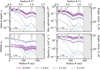 |
Fig. 5 Optical depth, absorption optical depth, albedo, and total dust opacity posterior distributions at 0.9, 1.3, 3.1, and 9.1 mm for our fiducial ‘Ricci (compact)’ composition. The solid lines and shaded regions display the median and 1σ uncertainty of each parameter. For comparison, the dotted lines show the results of the low resolution fit. The black dotted lines display the absorption optical depth estimated at each wavelength separately in the optically thin approximation from Equation (10). Our ALMA Band 6 surface brightness radial profile is plotted with grey dashed lines, the bright ring position is indicated and labelled as in the previous plots. The black and grey horizontal arrows mark the regions where the S/N of VLA Ka band surface brightness radial profile is >5 and 3. Dust emission is marginally optically thin at all the wavelengths. |
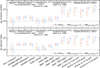 |
Fig. 6 Reduced χ2 between our model posteriors and the observed surface brightness (upper panel) or spectral index (bottom panel) radial profiles for different dust compositions, colour-coded by the outer-most disc radius the χ2 was averaged over. Mixtures including amorphous carbonaceous grains (e.g. ‘Ricci (compact)’ and ‘Zubko’) can fit our data the best. No constraints on the relative abundance of organics and other materials (especially water ice and silicates) can be drawn. |
5.3 Result comparison for different dust mixtures
To test the dependence of our results on the adopted dust mixture, we fitted CI Tau’s low resolution surface brightness profiles as in Section 4.3, ex novo adopting different sets of optical properties, generated using the dsharp_opac package (Birnstiel et al. 2018). Grains were assumed to be compact and spherical, their mixed dielectric constants were computed following the Bruggeman rule and their optical properties using Mie theory. To avoid artefacts due to poorly fitted temperature profiles, we fixed Tdust to be the temperature of a passively irradiated disc (as from Equation (E.1)) with flaring angle and luminosity matching the best-fit results of our fiducial case (i.e. ϕ = 0.035 and L⋆ = 1.04 L⊙). We evaluated the quality of these fits by comparing the reduced χ2 between our models and the surface brightness and spectral index radial profiles following the procedure introduced in Section 4.4. Figure 6 displays the median and 1σ uncertainty (defined as the range between the 16th and 84th percentiles) of the reduced χ2 posterior distributions for the different dust compositions we tested, colour-coded by the outermost disc radius ![Mathematical equation: $\[\chi_{\mathrm{SB}}^{2}\]$](/articles/aa/full_html/2025/10/aa52986-24/aa52986-24-eq44.png) (upper panel) and
(upper panel) and ![Mathematical equation: $\[\chi_{\mathrm{SI}}^{2}\]$](/articles/aa/full_html/2025/10/aa52986-24/aa52986-24-eq45.png) (bottom panel) were averaged over. Table K.5 summarises the mixtures and dielectric constants considered.
(bottom panel) were averaged over. Table K.5 summarises the mixtures and dielectric constants considered.
First of all, for our fiducial dust composition, Figure 6 shows that χ2 ≈ 1 with a small uncertainty (≲1 for R ≲ 82 au), thus confirming (see Appendix F) that ‘Ricci (compact)’ grains can fit remarkably well CI Tau’s surface brightness and spectral index radial profiles at most radii. We compared our fiducial results with those obtained using different dust optical properties, starting from the default mixture adopted by the DSHARP collaboration (Andrews et al. 2018; Birnstiel et al. 2018), labelled ‘DSHARP (default)’. In this case, while the brightness profiles are fitted reasonably well through all the disc ![Mathematical equation: $\[\left(\chi_{\mathrm{SB}}^{2} \approx 2\right)\]$](/articles/aa/full_html/2025/10/aa52986-24/aa52986-24-eq46.png) , αB7–B6 is systematically underestimated, leading to a larger
, αB7–B6 is systematically underestimated, leading to a larger ![Mathematical equation: $\[\chi_{\text {SI }}^{2} \approx 3\]$](/articles/aa/full_html/2025/10/aa52986-24/aa52986-24-eq47.png) for the spectral index radial profiles. This difference from our fiducial results does not depend on the different fraction of water ice adopted in the two mixtures, that only marginally affects dust optical properties (as already noticed by Birnstiel et al. 2018). Indeed, increasing the dust water ice content to 60% by volume (as in the ‘Ricci (compact)’ composition) or removing it altogether (compositions labelled ‘DSHARP (highwater)’ and ‘DSHARP (icefree)’, respectively), no clear difference from the ‘DSHARP (default)’ results can be seen in Figure 6, neither for the surface brightness, nor for the spectral index radial profiles.
for the spectral index radial profiles. This difference from our fiducial results does not depend on the different fraction of water ice adopted in the two mixtures, that only marginally affects dust optical properties (as already noticed by Birnstiel et al. 2018). Indeed, increasing the dust water ice content to 60% by volume (as in the ‘Ricci (compact)’ composition) or removing it altogether (compositions labelled ‘DSHARP (highwater)’ and ‘DSHARP (icefree)’, respectively), no clear difference from the ‘DSHARP (default)’ results can be seen in Figure 6, neither for the surface brightness, nor for the spectral index radial profiles.
Instead, the different organic materials (hence dielectric constants) adopted by Ricci et al. (2010b) and Birnstiel et al. (2018) impact our results the most. Depending on their synthesis temperature (e.g. Jäger et al. 1998), interstellar carbonaceous material can come in a mixture of different hybridisation states, such as sp2 (where sheets of carbon atoms are formed, as in graphite), sp3 (where carbon atoms are arranged in tetrahedral geometry, as in diamonds), or even mixed states (where curved structures, such as fullerene, are abundant). The relative fraction of these hybridisation states and the amount of hydrogenation heavily affect the dielectric constants of carbon grains (e.g. Zubko et al. 1996), with substantial effects on their opacities. To test the sensitivity of our results to these properties, following Birnstiel et al. (2018), we generate optical constants for dust mixtures with the same volume fractions as the ‘DSHARP (default)’ ones, but replacing the refractory organics with different carbonaceous materials8. First, we tested the dielectric constants of amorphous carbon grains produced by arc discharge in hydrogen atmosphere (ACH2-sample) or burning benzene (BE-sample) proposed by Zubko et al. (1996), labelled ‘Zubko (ACH2)’ and ‘Zubko (BE)’, respectively. In both cases, Figure 6 shows that our models are in excellent agreement with the data, with χ2 ≈ 1 and a small spread (≲ 1 for R ≲ 82 au) both for the surface brightness and spectral index radial profiles. Noticeably, as reported in Section 4.1 and Table K.5, also our fiducial ‘Ricci (compact)’ opacities were generated using the dielectric constants of Zubko et al. (1996) for ACH 2 amorphous carbon, further strengthening the evidence that amorphous carbon grains can fit our data remarkably well. The different fractions of mixing materials adopted in the ‘Ricci (compact)’ and ‘Zubko (ACH2)’ compositions, instead, suggests that (i) small fractions of troilite do not substantially affect our results, and (ii) our observations cannot discriminate between mixtures of the same materials in different fractions (within ≲ 15%), among those tested in Figure 6 (see Table K.5).
Instead, when the carbonaceous materials in the mixtures are made mostly by graphite, our models provide poorer fits to the data. This can be seen in Figure 6 when the refractory organics (Henning & Stognienko 1996) in the ‘DSHARP (default)’ mixture are replaced by carbonaceous materials synthesised by pyrolising cellulose at progressively higher temperatures (Jäger et al. 1998, labelled ‘Jäger’ followed by the pyrolysis temperature). Indeed, while organics produced by low temperature pyrolysis are made essentially by amorphous carbon and fit our data reasonably well (χ2 ≈ 2 to 3), at temperature higher than ≥800°C such grains become dominated by large graphitic areas and fit our data much worse (χ2 ≫ 5). Such low quality fits were also obtained adopting the graphite optical constants of Draine (2003, labelled ‘Draine’ followed by the carbon grain size and the relative direction of the electric field and the graphite plane our dielectric constants were computed for), confirming our hypothesis that mixtures including organics made by amorphous carbon can fit our data the best.
Such different results for different compositions can be explained by the Mie interference location and magnitude in their absorption opacity spectral index. In the case of ‘Ricci (compact)’, ‘Zubko’, and ‘DSHARP (default)’ compositions, such a resonance leads to a peak-like opacity spectral index profile, with βabs > 3 at amax ≈ λ/2π for q ≤ 2.5. Instead, for ‘Jäger (>800°C)’ and ‘Draine’ compositions, the opacity spectral index is sigmoid-shaped and ≤2.5, regardless of q. The number of resonances present varies from none up to a few, but they are low-amplitude and just make the βabs profile look more jagged. Since dust emission is optically thin in VLA Ka band (regardless of the compositions adopted in our analysis), only the former set of opacities can explain a βB3–Ka = αB3–Ka − 2 > 2.5 for R ≳ 30 au (see Figure 3). New (sub-)centimetre wavelength observations deep enough to detect dust emission with high S/N across the entire disc could provide stronger indications that αB3–Ka > 5 in the outer disc. This will be useful to further constrain dust composition because different peak magnitudes in the absorption spectral index can be seen between BE- and AC2H-sample amorphous carbon species (e.g. max(βabs) ≈ 4.3 and 4.7 for ‘Zubko (ACH2)’ and ‘Ricci (compact)’, while max(βabs) ≈ 3.3 for ‘Zubko (BE)’), but also for different water ice volume fractions (e.g. max(βabs) ≈ 3.9 for ‘DSHARP (icefree)’ opacities, while max(βabs) ≈ 3.1 for the ‘DSHARP (highwater)’ ones).
For the ‘Ricci (compact)’, ‘Zubko (BE)’, and ‘DSHARP (default)’ compositions we also performed high angular resolution fits as detailed in Section 4.3. Their marginalised posterior distributions are discussed in Appendix G and indicate that (i) the surface density and maximum grain size retrieved for the ‘Ricci (compact)’ and ‘Zubko (BE)’ mixtures are consistent within a factor of three, and (ii) the ‘DSHARP (default)’ mixture gives less reliable results.
To summarise, CI Tau’s curse of a steepening spectral index between ALMA Band 3 and VLA Ka band, which makes it difficult to detect and resolve dust emission at wavelengths longer than a few millimetres, turned out to be its blessing because only a few dust mixtures, those with the sharpest Mie resonance transition, such as ‘Ricci (compact)’ and ‘Zubko’, can explain this feature, providing unexpectedly strong constraints on the bulk dust composition in this disc.
5.4 Result comparison for different porosities
We tested the impact of dust porosity on our results fitting the low resolution surface brightness radial profiles with ‘Ricci’ and ‘DSHARP’ dust compositions, but progressively increasing their void fraction from 10%, 30%, 50%, and 70% up to 90% by volume9. We used the dsharp_opac package (Birnstiel et al. 2018) to determine the dielectric constants of each mixture with the Bruggeman rule10 and their optical properties using Mie theory for spherical grains. As for the comparison of different dust mixtures (Section 5.3), we kept the temperature fixed while fitting for the other parameters. Overall, for both the ‘Ricci’ and ‘DSHARP’ compositions we noticed an increase of the best-fit density and grain size with the porosity fraction, especially for filling factors >50% and >30% for the ‘Ricci’ and ‘DSHARP’ grain mixtures, respectively. This trend can be motivated by the reduced absorption opacity and the progressive shift of the Mie resonance to sizes much larger than the reference wavelength for fluffier particles.
To estimate the quality of these fits, we measured the reduced χ2 between our models and the surface brightness and spectral index radial profiles following the procedure introduced in Section 4.4. The median and 1σ uncertainty of the reduced χ2 posterior distributions as a function of the adopted porosity fraction, colour-coded by the outermost disc radius the χ2 was computed for, are displayed in Figure 7. The top and bottom panels summarise our model agreement with the surface brightness and spectral index radial profiles, respectively. Our fits with the ‘Ricci’ mixture (red, grey, and blue dots) can reproduce remarkably well both the brightness and spectral index profiles for compact grains and particles with porosity fractions up to 50%. In these cases, even though the estimated χ2 slightly increases with the void fraction, it remains below two. For every chosen porosity, the ‘DSHARP’ mixture (pink, grey, and green diamonds) fits our data worse than the ‘Ricci’ one, with χ2 > 3 already for void fractions as small as 10%. For both ‘Ricci’ and ‘DSHARP’ mixtures, porosities >50% lead to very poor quality fits. In addition for highly porous particles (with void fractions of 70% and 90% or larger, for the ‘DSHARP’ and ‘Ricci’ composition, respectively) our inferred dust density is so high that, for a standard dust-to-gas ratio Z = 10−2, CI Tau should be marginally gravitationally unstable (Toomre parameter Q < 1, grey shaded area in Figure 7). Since we observe no clear evidence of instability in the dust and gas emission, we favour lower porosity fractions.
The differences between ‘Ricci’ and ‘DSHARP’ results can be attributed once again to shape of the βabs profile. Increasing the porosity fraction in the dust mixture leads to progressively shallower Mie resonances in the absorption opacity spectral index (for a fixed q), that almost completely disappears for void fractions >50%. Therefore, the ‘DSHARP’ composition gives worse results than the ‘Ricci’ one because, for any given porosity, its optical properties lead to much shallower βabs profiles. They are so shallow that even reducing q (as in Figure G.1) does not provide enough flexibility to compensate for the effect of porosity on the Mie resonance. A similar justification applies to the case of ‘Ricci’ opacities with >70% porosity.
To summarise, dust porosity fractions up to ≈50% are compatible CI Tau’s observations when considering ‘Ricci’ opacities. The ‘DSHARP’ mixture, instead, provides good quality fits almost only for compact particles. This result suggests that, by robustly assessing the particle porosity (e.g. using full polarisation observations, see Section 6.2), we can tell ‘Ricci’ and ‘DSHARP’ opacity (or ultimately amorphous carbonaceous or refractory organic) models apart.
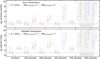 |
Fig. 7 Reduced χ2 between our model posteriors and the observed surface brightness (upper panel) and spectral index (bottom panel) radial profiles for different porosity fractions, colour-coded by the outermost disc radius the χ2 was averaged over. Dots and diamonds are used for the ‘Ricci’ and ‘DSHARP’ mixtures, respectively. The shaded grey regions indicate where the inferred dust surface density is high enough for the disc to be in the marginally gravitational unstable regime under the assumption of a standard dust-to-gas ratio Z = 10−2. The ‘Ricci’ mixture provides better fits than the ‘DSHARP’ one for every porosity level and suggests that dust in CI Tau can be up to 50% porous. The ‘DSHARP’ mixture, instead, can explain the data only for compact aggregates. |
6 Discussion
6.1 Interpretation of the best-fit radial profiles
Maximum grain size. A puzzling result from Section 5.1 is our smooth and almost constant best-fit grain size radial profile.
As noticed by Jiang et al. (2024), smooth maximum grain size radial profiles are common to almost all the discs targeted by previous studies similar to ours. Based on the results of dust coagulation and transport simulation, they suggested that, even in the presence of low levels of turbulence (αturb ≈ 10−4), fragile pebble collisions (i.e. with a low fragmentation velocity threshold of ufrag ≈ 1 × 102 cm s−1) make dust growth fragmentation-limited through the whole disc extent. While this argument qualitatively explains the absence of peaks and troughs in our maximum grain size radial profile, under the commonly adopted assumption that the gas surface density declines more steeply than the temperature radial profile, it requires turbulence to decrease radially. In fact, since, in the fragmentation-dominated regime, afrag ∝ Σgas/(αturbTdust), where Σgas is the gas surface density (Birnstiel et al. 2012), if the gas surface density and temperature can be expressed as power law functions of the disc radius with exponent γ and p, where γ < p, then the turbulence will decrease radially as γ − p = γ + 0.5 < 0. In Appendix H we discuss more in detail the turbulence levels expected of CI Tau if amax = afrag and for a standard dust-to-gas ratio, Z = 10−2.
Alternatively, the very weak radial dependence of the maximum grain size in CI Tau could be the consequence of particle bouncing. In fact, since the bouncing velocity threshold depends on the particle mass, the bouncing barrier is almost radially flat (e.g. in the simulations of Stammler et al. 2023 and Birnstiel 2024, amax ∝ (R/10 au)−3/16, in excellent agreement with our results). Furthermore, it scales much more weakly with Σgas and αturb then the fragmentation barrier (![Mathematical equation: $\[a_{\text {boun }} \propto a_{\text {frag }}^{1 / 4}\]$](/articles/aa/full_html/2025/10/aa52986-24/aa52986-24-eq48.png) , Dominik & Dullemond 2024), thus requiring less stringent constraints on their radial profiles. However, we caveat against a straightforward interpretation of our results in favour of the bouncing and against the fragmentation barrier for two main reasons. First, despite having been considered only rarely in collisional models (e.g. Windmark et al. 2012), it has been proposed that also the fragmentation velocity threshold (Beitz et al. 2011) and the dust tensile strength (San Sebastián et al. 2020) depend on the particle mass. Secondly, it could be possible that our fit would not be able to recover a radial decrease of the maximum grain size, even if genuinely present, because of the limited quality of our VLA Ka band data. Deeper (sub-)centimetre wavelength observations able to confirm that continuum emission is detected out to ≲200 au are crucial to support our results.
, Dominik & Dullemond 2024), thus requiring less stringent constraints on their radial profiles. However, we caveat against a straightforward interpretation of our results in favour of the bouncing and against the fragmentation barrier for two main reasons. First, despite having been considered only rarely in collisional models (e.g. Windmark et al. 2012), it has been proposed that also the fragmentation velocity threshold (Beitz et al. 2011) and the dust tensile strength (San Sebastián et al. 2020) depend on the particle mass. Secondly, it could be possible that our fit would not be able to recover a radial decrease of the maximum grain size, even if genuinely present, because of the limited quality of our VLA Ka band data. Deeper (sub-)centimetre wavelength observations able to confirm that continuum emission is detected out to ≲200 au are crucial to support our results.
Nevertheless, some sources show different trends, with significant increases of amax at the position of some bright rings. Examples are the 100 au ring in HD 163296 (Sierra et al. 2021, but we note that the analysis of Guidi et al. 2022, which is based on higher angular resolution observations over a broader frequency range, disputed this claim), some rings in HL Tau (Carrasco-González et al. 2019, but see the updated model of Guerra-Alvarado et al. 2024, whose maximum grain size radial profile is less substructured, within the uncertainties11) and TW Hya (Macías et al. 2021). However, in all of these cases, a fixed power-law density distribution (q = 2.5 by Sierra et al. 2021, and q = 3.5 by Carrasco-González et al. 2019, Guerra-Alvarado et al. 2024 and Macías et al. 2021) was adopted.
To better compare these results with ours, we also ran a set of low resolution fits fixing q = 3.5 (the typical size distribution exponent of the ISM dust Mathis et al. 1977, that also lies in the range of values constrained by our fit, as shown in the bottom-right panel of Figure 4) and q = 2.5 (that spans a much wider range of absorption opacity spectral indices, βabs, thus providing lower limits on amax, as noticed by Sierra et al. 2021). However, neither option can fit the data well because our prescription is not flexible enough to explain both the spectral index at ALMA wavelengths and between ALMA Band 3 and the VLA Ka band data, that provide a crucial additional constraint when compared with the results of Macías et al. (2021) and Sierra et al. (2021), based on ALMA-only data12. Interestingly, Macías et al. (2021) fitted their data also leaving q as a free parameter. In this case, they obtained much more similar results to ours: an almost constant amax profile with radius, albeit with a larger uncertainty, and a density distribution power-law index radial profile that decreases towards the inner disc and at the position of the bright rings.
Grain size distribution. In contrast with the maximum grain size radial profile, our dust density distribution decreases towards the inner disc and at the location of the bright rings. We stress that, in the absence of radial variations of amax, the dependence of q on the disc radius is essential to explain the radial increase of CI Tau’s spectral indices (see Figure 3), which, according to our models, reflects a similar increase of the absorption spectral index, as is show in Appendix I. These features suggest that a larger fraction of the dust distribution is dominated by the largest particles (i.e. those with size ≈amax) in the inner disc and the bright rings.
In the outer disc, our best-fit dust size distribution is broadly consistent with the expectations of fragmentation-limited growth (q = 3.5, Birnstiel 2024, see also the more-refined predictions for a fragmentation-coagulation equilibrium of Birnstiel et al. 2011). Instead, in the inner disc, q lies between the values expected when the maximum grain size is limited by the fragmentation and the radial drift threshold (q = 2.5, Birnstiel 2024). Such a best-fit dust number density distribution is also not consistent with the results of bouncing-limited dust growth simulations, that predict an almost monodisperse particle size distribution (Stammler et al. 2023; Dominik & Dullemond 2024; Birnstiel 2024). Nevertheless, such predictions are based on models that did not consider processes, such as erosion by abrasion, that are detrimental to growth and could substantially increase the fraction of small particles, thus widening the dust size distribution and increasing q (Dominik & Dullemond 2024). Dedicated collisional growth and dust transport simulations are needed to interpret our results self-consistently. As for the rings, instead, in the fragile pebble collision scenario discussed above (i.e. where rings are not favourable locations for dust to grow), the lower q could be explained by the preferential confinement of larger grains in pressure bumps co-located with the rings (Pinilla et al. 2012). In fact, smaller and better-coupled solids, that are more easily diffused away or mixed up by turbulence, can filter through a pressure maximum (e.g. Petrovic et al. 2024), locally increasing the fraction of larger particles.
To summarise, our results suggest that turbulent fragmentation or bouncing are the dominant processes halting dust growth in CI Tau. On top of this global trend, dust confinement in the rings provides a possible explanation for the small-scale modulations of the dust density and grain size power law index radial profiles. Deeper (sub-)centimetre observations, able to detect continuum emission with higher S/N in the outer disc or provide stringent upper limits, are essential to reassess this picture.
6.2 Dust polarisation and the role of porosity
As an alternative to the multi-frequency continuum analysis we presented in this paper, (multi-wavelength) linear polarisation observations have also been used to provide constraints on the properties of dust in planet-forming discs (e.g. Miotello et al. 2023). Over the last decade, linear polarisation fractions of about 1% have been detected in a number of sources, such as HL Tau (Stephens et al. 2017), HD 163296 (Dent et al. 2019), HD 142527 (Kataoka et al. 2016), IM Lup (Hull et al. 2018), CW Tau and DG Tau (Bacciotti et al. 2018). At 0.9 mm, the polarisation vectors are most often oriented along the disc minor axis. This polarisation pattern is commonly interpreted as due to dust self-scattering (Kataoka et al. 2015). However, 1.3 and 3.1 mm observations revealed that the polarisation pattern can be frequency-dependent (e.g. Stephens et al. 2017), with polarisation vectors being progressively more azimuthally aligned at longer wavelengths, suggesting that other processes, such as dust grain alignment with the radiation field (Tazaki et al. 2017), become the dominant source of polarisation. The (wavelength dependence of the) polarisation fraction due to self-scattering can be used to provide estimates of the maximum grain size by comparison with model predictions (Kataoka et al. 2015), as in the case of HL Tau, where the decrease of self-scattering polarisation with wavelength was interpreted by Kataoka et al. (2017) as a strong evidence that only grains of amax ≲ 100 μm are present in the disc, in puzzling contrast with the results of the analysis of multi-frequency continuum observations of the same source (Carrasco-González et al. 2019; Guerra-Alvarado et al. 2024).
Several explanations were put forward to account for this discrepancy, such as dust vertical settling and optical depth effects (Lin et al. 2020; Ueda et al. 2021, but see Sierra & Lizano 2020 for a counter-argument), the different nature of continuum and polarised-light emission (e.g. signal contamination by polarisation due to alignment of oblate dust with the magnetic or radiation field, Kirchschlager & Bertrang 2020), or dust composition (Yang & Li 2020 suggested that adopting dust mixtures including amorphous carbonaceous grains instead of refractory organics might alleviate the tension between the results of polarised-light and continuum observation analyses). Following Tazaki et al. (2019), who noticed that the range of particle sizes with high self-scattering polarisation fraction is wider for porous grains than compact particles, Zhang et al. (2023) proposed that particles with 70% to 97% porosity can explain both the dust continuum and linear polarisation multi-frequency observations of HL Tau. Similar porosity fractions of 80% were shown to be in remarkable agreement with scattered light and (sub-)millimetre (continuum and linear polarisation) observations of IM Lup by Ueda et al. (2024).
Unfortunately, full polarisation observations of CI Tau have never been taken, and no information on the dust polarisation fraction in this disc is available. As a consequence, all our constraints on particle porosities are based on our continuum profile analysis in Section 5.4. Our preference for low porosity fractions in CI Tau is in contrast with the aforementioned results of Zhang et al. (2023) and Ueda et al. (2024) in HL Tau and IM Lup, even more so since they adopted the default ‘DSHARP’ mixture, that provides good quality fits to our data almost only in the compact case. Instead, our results are consistent with those of Guidi et al. (2022), whose multi-frequency continuum observations of HD 163296 can be better explained by low particle porosities (25% instead of 80%). While both our analysis and that of Guidi et al. (2022) did not consider polarisation observations, and therefore provided more uncertain estimates of the dust porosity, it is likely that the differences between the porosity fractions of HL Tau/IM Lup and CI Tau/HD 163296 are real. Indeed, while the former sources are known to be very young (≲1 Myr, e.g. Alcalá et al. 2017), the latter are relatively (CI Tau, >3 Myr, Gangi et al. 2022) to significantly (HD 163296, ≳6 Myr, Fairlamb et al. 2015) older. Thus, it can be speculated that time-dependent processes (e.g., dust compaction) might have played a role in determining those differences.
Both laboratory experiments and numerical simulations suggest that the initial stages of particle growth take place by hit-and-stick, a process that leads to very fluffy aggregates with low fractal dimensions (see e.g. Testi et al. 2014, and references therein). Subsequently compaction is thought to take place: the fractal dimension increases and the porosity decreases up to 40 to 60% due to a combination of bouncing- and fragmentation-driven compression (Michoulier et al. 2024). On the one hand, the high porosity fractions inferred in HL Tau and IM Lup are more in line with the models of Ginski et al. (2023), who showed that the small particles in the upper disc layers probed by scattered light observations are very porous or have small fractal dimensions. This suggests that dust in these young discs is still growing or undergoing compression. On the other hand, our results for CI Tau and those of Guidi et al. (2022) for HD 163296 are more consistent with the models of Rosotti et al. (2019a); Zormpas et al. (2022); Delussu et al. (2024), that showed that compact grains can better reproduce the size luminosity correlation detected at (sub-)millimetre wavelengths in nearby 1–3 Myr-old star-formation regions. This being said, the porosity fraction that particles can reach after compaction depend on a number of disc parameters, such as the radial location (because of the different collisional timescale and dust-to-ice ratio, e.g. Lorek et al. 2018, and Michoulier et al. 2024). Thus the observed differences, if confirmed, might also reflect more intrinsic source differences than a genuine time-dependent process.
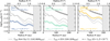 |
Fig. 8 Comparison between the pebble masses (top-left corner, within R < 200 au) inferred from the dust surface density radial profiles fitted using different compositions (for compact grains only). The solid and dashed grey lines display the expected dust surface density radial profiles obtained by converting the ALMA Band 6 surface brightness radial profile using a constant temperature of 20 K and the temperature profile from Equation (E.1), both for κ230 GHz = 2.3 cm2 g−1. The median absorption opacity from our multi-wavelength fit for different dust mixtures is annotated in the bottom-left corner of each subplot. The dashed-dotted black line shows the upper limit on the dust surface density, corresponding to a Toomre parameter Q = 1 and a gas-to-dust ratio Z = 10−2. |
6.3 Pebble mass estimates
Knowledge of the disc dust mass is crucial to determine the potential of a disc to form (new) planets. Being sensitive to small solids, but blind to the dust sequestered in larger aggregates, such as planetesimals and planetary cores, continuum observations in the (sub-)millimetre have been traditionally used to provide lower limits on the disc dust mass, under the assumption that continuum emission at these wavelengths is optically thin, as (Hildebrand 1983)
![Mathematical equation: $\[M_{\mathrm{dust}} \geq M_{\mathrm{pebb}} \approx \frac{F_\nu d^2}{\kappa_\nu B_\nu\left(T_{\mathrm{dust}}\right)},\]$](/articles/aa/full_html/2025/10/aa52986-24/aa52986-24-eq49.png) (11)
(11)
where Fν is the disc dust flux density at frequency ν and d is the source distance, adopting a fiducial opacity (κν ≈ 2.3 cm2 g−1 at 230 GHz, see e.g. Ansdell et al. 2016, 2018; Pascucci et al. 2016; Barenfeld et al. 2016) and dust temperature (Tdust = 20 K, see e.g. Ansdell et al. 2016, 2018, sometimes rescaled by the stellar luminosity, e.g. Pascucci et al. 2016; Barenfeld et al. 2016). We refer to this lower limit as pebble mass, Mpebb.
Over the last years, it was realised that the pebble masses inferred from (sub-)millimetre surveys in nearby star-formation regions were not high enough (Manara et al. 2018) or barely sufficient (Najita & Kenyon 2014; Mulders et al. 2021) to form the rocky cores of the currently detected exoplanets. A number of solutions to this ‘mass budget’ problem were proposed, such as the presence of highly optically thick regions capable of hiding large pebbles mass fractions (e.g. Zhu et al. 2019; Ribas et al. 2020), the possibility that planetary cores form much earlier than the Class II stage (e.g. Tychoniec et al. 2020), or, more recently, the replenishment of fresh ISM material (e.g. Winter et al. 2024).
Multi-frequency continuum observations can provide more reliable estimate of the pebble mass in a disc because of their accurate constraints on the dust optical depth and mid-plane temperature. Figure 8 displays a comparison between the pebble masses inferred for the ‘Ricci (compact)’, ‘Zubko (BE)’, and ‘DSHARP (default)’ compositions in CI Tau and the results obtained under the traditional optically thin and fixed temperature assumptions. The dust surface densities posterior distributions from our high resolution multi-frequency fits for the aforementioned compositions are displayed in each subplot in blue, turquoise, and yellow, respectively. On top of these profiles, we also plotted the dust surface density estimated from the ALMA Band 6 surface brightness radial profile, under the assumption of optically thin emission, defined as (Equation (10), for ![Mathematical equation: $\[\tau_{\nu}^{\mathrm{abs}} \ll 1\]$](/articles/aa/full_html/2025/10/aa52986-24/aa52986-24-eq50.png) )
)
![Mathematical equation: $\[\Sigma_{\mathrm{dust}, \mathrm{OT}}=\frac{I_\nu}{B_\nu} \frac{\cos~ i}{\kappa_\nu}.\]$](/articles/aa/full_html/2025/10/aa52986-24/aa52986-24-eq51.png) (12)
(12)
We adopted the same opacity law traditionally used to convert dust flux densities into dust masses: i.e. κν is 2.3 cm2 g−1 at 230 GHz (Ansdell et al. 2016) and scales linearly with frequency (Beckwith et al. 1990). Solid and dashed grey lines were used for a constant temperature of 20 K and the temperature profile of a passively irradiated disc (Equation (E.1), with ϕ = 0.035 and L⋆ = 1.04 L⊙), respectively. Finally, the dashed-dotted black curves show the dust surface density profile corresponding to a Toomre parameter Q = 1 (Toomre 1964) for a standard dust-to-gas ratio Z = 10−2:
![Mathematical equation: $\[\Sigma_{\text {dust }, \mathrm{Q}}=\frac{c_{\mathrm{s}} \Omega_{\mathrm{K}} Z}{\pi G},\]$](/articles/aa/full_html/2025/10/aa52986-24/aa52986-24-eq52.png) (13)
(13)
where cs is the locally isothermal sound speed (computed with a mean-molecular mass of μ = 2.4), ΩK is the Keplerian angular velocity (estimated for a central mass of M⋆ = 1.29 ± 0.45 M⊙ Gangi et al. 2022), and G is the gravitational constant.
As is clear from Figure 8, different assumptions on dust composition provide different estimates of the pebble mass in the disc. The masses estimated under the traditional optically thin assumption, regardless of the temperature being 20 K (grey solid line) or decreasing with radius (grey dashed line), are a factor of two lower than those based on the ‘DSHARP (default)’ opacity fit, but overestimate those measured from the ‘Ricci (compact)’ and ‘Zubko (BE)’ best-fit surface density profiles by a factor of three to five. This naively gives credit to the realisation, dating back to the work of Beckwith et al. (1990), that knowledge of the dust composition is crucial to provide reliable constraints on the pebble mass. Our marginal preference for ‘Ricci (compact)’ and ‘Zubko (BE)’ opacities over the ‘DSHARP (default)’ ones, extensively motivated in the previous sections, has two main consequences. Firstly, if taken at face value, the pebble mass comparison shown in Figure 8 suggests that, under standard assumptions on opacity and temperature, Equation (11) does not always underestimate the dust mass, as is often assumed13. Secondly, it would suggest that, if giant planet formation occurred in CI Tau, this process might be already over. This is supported by current estimates of the total mass of heavy elements in Solar System giants, thought to be 8 to 46 MEarth in Jupiter and 16 to 30 MEarth in Saturn (Guillot et al. 2023 and references therein), and thus in line or higher than the pebble mass in CI Tau measured for ‘Ricci (compact)’ and ‘Zubko (BE)’ dust mixtures. Clearly, the (still poorly constrained) dust porosity fraction adds to the previously mentioned sources of uncertainty. However, for the ‘Ricci’ mixture, the pebble mass inferred from our multi-wavelength analysis does not exceed Mpebb ≈ 134.39 MEarth for a 50% porosity fraction. This value does make it more feasible to assemble the core of a new gas giant in the system with a more reasonable, but still high (Drążkowska et al. 2023), efficiency of ≈30%.
Finally, in Table K.6 we compare our results for CI Tau with similar estimates of the pebble mass from 1.3 mm continuum observations and multi-frequency observations in the literature. Our results for ‘DSHARP (default)’ opacities for CI Tau are in line with those obtained in all the other sources with the exception of IM Lup, that is more massive and potentially marginally gravitationally unstable, as it might be hinted by the m = 2 spiral detected in (sub-)millimetre continuum observations (Huang et al. 2018b) and its high gas mass inferred from a kinematic analysis of its super-Keplerian rotation curve (Martire et al. 2024). This is suggesting that adopting our fiducial ‘Ricci (compact)’ composition also for these sources, will likely decrease their pebble masses and planet-formation potential (see Sierra et al. 2025 for LkCa 15).
7 Summary and conclusions
We have introduced, for the first time, deep ALMA Band 3 and VLA Ka, Ku, X, and C band continuum observations of CI Tau. We took advantage of the high angular resolution and sensitivity of ALMA Band 3 and VLA Ka band observations and of combining them with similar quality archival ALMA Band 6 and 7 data to study the properties of dust in this system. Our main results are summarised in the following list:
At ALMA wavelengths, continuum emission towards CI Tau displays similar morphologies, characterised by a sequence of three gaps and four rings, as previously reported by Clarke et al. (2018) and Long et al. (2018) at 1.3 mm and Rosotti et al. (2021) at 0.9 mm. Non-parametric modelling of the visibilities (with the code frank) revealed that the innermost bright ring is substructured (i.e. made of two sub-beam rings and a gap in between) and highlighted the presence of an additional gap at ≈5 au in the 1.3 mm data (see also Jennings et al. 2022b);
In contrast, the VLA Ka band emission is very faint and shows no clear substructures, not even in the best-fit frank profile. When reconstructed with a large-enough beam (>
![Mathematical equation: $\[0^{\prime\prime}_\cdot150\]$](/articles/aa/full_html/2025/10/aa52986-24/aa52986-24-eq53.png) ), extended emission can be detected, as can also be seen in the best-fit frank profile, albeit at a low S/N ≈ 3;
), extended emission can be detected, as can also be seen in the best-fit frank profile, albeit at a low S/N ≈ 3;CI Tau’s integrated spectral index between 0.9 and 3.1 mm is 2.6 ± 0.1, which is in line with those measured in HL Tau, TW Hya, and HD 163296. Between 3.1 and 9.1 mm, the spectral flux density distribution steepens, with an integrated spectral index of 4.3 ± 0.2, and is thus significantly larger than in the previously mentioned sources. At even longer wavelengths, emission is not dominated by dust but likely by a combination of optically thick gyrosynchrotron emission (at λ ≳ 2 cm), as suggested by the high X band flux density variability and optically thin free-free emission (at λ ≲ 1 cm). Deeper (sub-)centimetre simultaneous observations (e.g. from C to Q band) probing variability on longer timescales are needed to conclusively assess the nature of CI Tau’s continuum radio emission;
We developed a two-step Bayesian method to model CI Tau’s surface brightness radial profiles. First, the observations between 0.9 and 9.1 mm were fitted at low resolution (
![Mathematical equation: $\[0^{\prime\prime}_\cdot195\]$](/articles/aa/full_html/2025/10/aa52986-24/aa52986-24-eq54.png) ). These results where then used as priors for a high-resolution (
). These results where then used as priors for a high-resolution (![Mathematical equation: $\[0^{\prime\prime}_\cdot058\]$](/articles/aa/full_html/2025/10/aa52986-24/aa52986-24-eq55.png) ) fit only to the ALMA data. This new technique allows one to trade off resolution for sensitivity in centimetre-wavelength observations, where targets are generally very faint and long integration times are required to get good quality data;
) fit only to the ALMA data. This new technique allows one to trade off resolution for sensitivity in centimetre-wavelength observations, where targets are generally very faint and long integration times are required to get good quality data;When adopting the ‘Ricci (compact)’ bulk composition, our best-fit dust temperature profile is smooth and radially declines as expected for a passively irradiated disc. The dust surface density profile increases, while q (the slope of the dust density distribution, i.e. the fraction of small grains) decreases locally at the position of the bright rings, which is in line with the predictions of dust trapping simulations. Our best-fit maximum grain size, however, is smooth and radially flat, as expected from models of fragile dust collisions in low-turbulence discs or bouncing-limited dust growth. Our analysis revealed that CI Tau’s continuum emission is optically thin between 0.9 and 9.1 mm, in contrast with most of the sources previously studied with similar quality multi-wavelength observations;
For compact grains, we tested the dependence of our results on dust composition, comparing the χ2 between the observed and predicted surface brightness and spectral index radial profiles. We showed that the fraction of water ice included in the mixture only negligibly affects the goodness of the fit, while changing the refractive constants of organics leads to substantial differences. In particular, our data disfavour graphite-dominated carbon and marginally prefer amorphous carbonaceous grains (Zubko et al. 1996) over refractory organics (Henning & Stognienko 1996). Deeper (sub-)centimetre wavelength data are needed to confirm our results. The different optical depths expected in the case of ‘Ricci (compact)’ and ‘DSHARP (default)’ mixtures provide an additional opportunity to constrain internal composition with independent estimates of the total dust extinction (see Appendix G);
For a fixed particle composition, we tested the dependence of our results on dust porosity using the same χ2 comparison method. We showed that the ‘Ricci’ mixture can fit the data well for void fractions up to 50%, while for porosities larger than 70%, it leads to worse results. This is in contrast with the recent inferences of high porosity fraction (80 to 90%) in the younger HL Tau and IM Lup discs. This difference could be attributed to time-dependent compaction, but dedicated models are needed to confirm this hypothesis. Increasing the void fraction, the ‘Ricci’ mixture performs progressively better than the ‘DSHARP’ one. Deeper (sub-)centimetre continuum and (multi-wavelength) polarisation observations are needed to confirm our results and better constrain particle porosity. Given the increasingly different behaviour of the ‘Ricci’ and ‘DSHARP’ compositions for larger void fractions, knowledge of porosity could also be used to better constrain the bulk dust composition;
For our fiducial ‘Ricci (compact)’ composition, we estimated CI Tau’s pebble mass to be Mpebb =
![Mathematical equation: $\[31.13_{-6.00}^{+8.77}\]$](/articles/aa/full_html/2025/10/aa52986-24/aa52986-24-eq56.png) MEarth, thus a factor of three to five lower than expected from the dust luminosity conversion traditionally employed in snapshot surveys (Equation (11)). This difference is primarily driven by the adopted absorption opacities, which are much higher for ‘Ricci (compact)’ grains (
MEarth, thus a factor of three to five lower than expected from the dust luminosity conversion traditionally employed in snapshot surveys (Equation (11)). This difference is primarily driven by the adopted absorption opacities, which are much higher for ‘Ricci (compact)’ grains (![Mathematical equation: $\[\langle\kappa_{230 \mathrm{GHz}, \mathrm{fit}}^{\mathrm{abs}}\rangle=11.9 \mathrm{~cm}^{2} \mathrm{~g}^{-1}\]$](/articles/aa/full_html/2025/10/aa52986-24/aa52986-24-eq57.png) , mediated over our amax and q posteriors) than is commonly assumed (
, mediated over our amax and q posteriors) than is commonly assumed (![Mathematical equation: $\[\kappa_{230 \mathrm{GHz}}^{\mathrm{abs}}=2.3 \mathrm{~cm}^{2} \mathrm{~g}^{-1}\]$](/articles/aa/full_html/2025/10/aa52986-24/aa52986-24-eq58.png) ). Such a low pebble mass is barely enough to account for the heavy element mass in Jupiter or Saturn. This suggests that if giant planet formation is taking place in CI Tau, the rocky cores of such planets mostly likely have already been assembled. Compared to other more optically thick sources, uncertainties on the bulk composition rather than optical depth corrections dominate our uncertainty on the pebble mass estimate in CI Tau.
). Such a low pebble mass is barely enough to account for the heavy element mass in Jupiter or Saturn. This suggests that if giant planet formation is taking place in CI Tau, the rocky cores of such planets mostly likely have already been assembled. Compared to other more optically thick sources, uncertainties on the bulk composition rather than optical depth corrections dominate our uncertainty on the pebble mass estimate in CI Tau.
Deeper (sub-)centimetre observations (e.g. with ALMA in Band 1) and follow-up polarisation observations, are needed to confirm our preference for amorphous carbonaceous grains with low porosities. Expanding our analysis to other sources, especially moderate-to-low optical depth discs such as AS 209 or GM Aur (Sierra et al. 2021), could be ideal to further test different dust composition models and, by comparison with our results for CI Tau, understand if composition and porosity change from source to source. Future facilities, first and foremost the next generation Very Large Array (ngVLA), will be crucial to obtaining better resolution and sensitivity centimetrewavelength observations and to extending our analysis to larger samples.
Acknowledgements
This paper makes use of the following ALMA data: ADS/JAO.ALMA#2015.1.01207.S, ADS/JAO.ALMA#2016.1.01370.S, ADS/JAO.ALMA#2017.A.00014.S, and ADS/JAO.ALMA#2018.1.00900.S, ALMA is a partnership of ESO (representing its member states), NSF (USA), and NINS (Japan), together with NRC (Canada), NSC and ASIAA (Taiwan), and KASI (Republic of Korea), in cooperation with the Republic of Chile. The Joint ALMA Observatory is operated by ESO, AUI/NRAO, and NAOJ. This paper makes use of the following VLA data: VLA/19A-440 and VLA/20A-373. The National Radio Astronomy Observatory (NRAO) is a facility of the National Science Foundation operated under cooperative agreement by Associated Universities, Inc. FZ acknowledges support from STFC and Cambridge Trust for a Ph.D. studentship, is grateful to the Institute for Astronomy, University of Hawai’i at Manoa, for hosting him for a Dustbusters secondment when this project came to be. FZ thanks Til Birnstiel, Ted Bergin, Greta Guidi, Oliver Shorttle, Elena Viscardi, and Mark Wyatt for insightful discussions on dust properties and the analysis method. SF is funded by the European Union (ERC, UNVEIL, 101076613), and acknowledges financial contribution from PRIN-MUR 2022YP5ACE. PC acknowledges support by the Italian Ministero dell Istruzione, Università e Ricerca through the grant Progetti Premiali 2012 – iALMA (CUP C52I13000140001) and by the ANID BASAL project FB210003. A.R. has been supported by the UK Science and Technology Facilities Council (STFC) via the consolidated grant ST/W000997/1. RAB is supported by a University Research Fellowship. GR is funded by the European Union under the European Union’s Horizon Europe Research & Innovation Programme No. 101039651 (DiscEvol) and by the Fondazione Cariplo, grant no. 2022-1217. Views and opinions expressed are however those of the author(s) only and do not necessarily reflect those of the European Union or the European Research Council. Neither the European Union nor the granting authority can be held responsible for them. This project has received funding from the European Union’s Horizon 2020 research and innovation programme under the Marie Sklodowska-Curie grant agreement No. 823823 (Dustbusters RISE project). Software: CASA v6.4.3.27 and 6.2.1.7 (McMullin et al. 2007; CASA Team 2022), analysisUtils (Hunter et al. 2023), gofish v1.4.1 (Teague 2019), frank (Jennings et al. 2020), uvplot (Tazzari 2017), corner v2.2.1 (Foreman-Mackey 2016), emcee v3.1.2 (Foreman-Mackey et al. 2013, 2019), numpy v1.24.2 (Harris et al. 2020), scipy v1.10.1 (Virtanen et al. 2020), matplotlib v3.7.1 (Hunter 2007), astropy v5.2.1 (Astropy Collaboration 2013, 2018, 2022), JupyterNotebook v6.5.2 (Kluyver et al. 2016), dsharp_opac v1.1.4 (Birnstiel et al. 2018). Scripts and data are publicly available on GitHub.
Appendix A ALMA flux density calibration
Before concatenation, the visibilities of all the ALMA datasets in the same band were deprojected and inspected to identify any mismatches in the amplitude scales. These mismatches were then corrected for by rescaling the flux densities of all the EBs at the same frequency to that of the reference one, using the gencal task. This reference observing block was selected by comparing the observed luminosity of each flux calibrator with that interpolated from their tabulated light curves at the same epoch. Hereafter we discuss how the reference EB was determined for each band.
Figure A.1 and A.2 display the light curves (both tabulated and interpolated) of the flux calibrators targeted during ALMA Band 7, 6, and 3 observations. Different subplots refer to a different observing block and hence to a different flux calibrator or observing time. In each subplot, the tabulated flux densities14 are shown as hollow dots over a timescale of four months around the observation date. Yellow and green colours were used for Band 3 measurements, cyan for the Band 7 ones. The larger, full dots, instead, display the expected luminosities of the flux calibrators at a fixed cadence of three days. These were computed at the frequency of one of the SPWs in the observations (see captions), interpolating between the closest tabulated Band 3 and 7 flux densities, using the au.getALMAFlux task (Hunter et al. 2023). These dots are colour-coded by the epoch offset from (i.e. number of days before or after) the closest tabulated flux density measurements in Band 3 (top-half) and 7 (bottom-half of the dot). Black crosses display the observed luminosity of each flux calibrator in the same SPW the expected luminosities were interpolated at.
ALMA Band 7 – The two EBs in Band 7 were observed the same day (11 December 2017). Their flux densities differ by ≈5% and the luminosities of their flux calibrator (J0510+1800) are within ≲ 6% of their closest tabulated flux density measurements (see top panel of Figure A.1), consistent with the 10% (2σ) absolute flux density accuracy reported in the ALMA Technical Handbook15. Since the two measurements are essentially identical, we selected the latest one as the reference EB.
ALMA Band 6 – The long and short baseline observations in Band 6 were taken one year apart (27 August 2016 for the SBs and 23 and 24 September 2017 for the LBs). Their average frequencies are also slightly different (225.6 GHz for the SBs and 233.0 GHz for the LBs), complicating the comparison. As for the SBs, the luminosity of its flux calibrator (J0510+1800) is within ≲ 5% of the expected one interpolated from its closest tabulated measurement in Band 3 and 7 (see bottom panel of Figure A.1), consistent with the 10% (2σ) absolute flux density accuracy reported in the ALMA Technical Handbook. However, the tabulated measurements were taken 7 days before (Band 3) and 6 days after (Band 7) our observations. Reassuringly, CI Tau’s SB flux density is in excellent agreement (difference ≈1%) with the one reported by Long et al. (2018) using data from the program 2016.1.01164.S (PI: G. Herczeg) at a very similar reference frequency (difference < 1%). The 2016.1.01164.S data were taken the same day (27 August 2017) of a tabulated measurement of the luminosity of their flux calibrator (J0510+1800). Their observed and tabulated flux densities agree within < 1%. Therefore, we are confident that our SB data were flux calibrated accurately. However, since their average frequency is lower than that of the LB data, using the SBs as our reference EB would systematically underestimate the Band 6 luminosity.
Despite having been observed only one day apart, the flux densities of the two LB execution blocks differ by more than 10%. The luminosity of the EB observed on 23 September (hereafter LB0) is 175.55 mJy, while that of the EB observed the day after (hereafter LB1) is 155.63 mJy. The first would imply an intraband (i.e. with respect to the SB data) spectral index of 6.9 ± 4.4, while the second is consistent with the spectral index between the Band 6 SB and Band 7 data. In addition to these considerations, we chose LB1 as reference EB for its better uv-coverage at short baselines, and rescaled the LB0 luminosity to the LB1 one. Curiously, though, the luminosity of the LB0 flux calibrator perfectly matches the expected one, while that of the LB1 differs by more than 10% (see central panel of Figure A.1). This is likely due to the calibrator progressively dimming between September and November 2017, and the closest tabulated measurements of its luminosity being taken 7 days after (Band 3) and 3 days before (Band 7) our observations.
ALMA Band 3 – The three EBs in Band 3 were observed more than two years apart (27 June and 4 July 2019, 3 July 2021). Their flux density ratios are ≲ 4% and the luminosities of their flux calibrators (J0423-0120, J0510+1800, and J0237+2848) are ≲ 1% of their closest tabulated flux density measurements (see Figure A.2), consistent with the 5% (2σ) absoluteflux density accuracy reported in the ALMA Technical Handbook. Since the same day of our observations conducted on 4 July 2019 a tabulated measurement of the luminosity of the flux calibrator J0510+1800 is available and it agrees within ≲ 1% with the observed one, we selected this EB as the reference one.
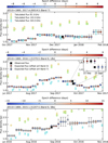 |
Fig. A.1 Light curves of the flux calibrators (Band 6 and 7). The expected flux densities were interpolated at 330.7, 242.0, and 234.4 GHz, respectively. The insert shows the one-day cadence interpolation for the week LB data were taken. |
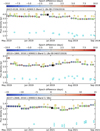 |
Fig. A.2 Light curves of the flux calibrators (Band 3). Expected flux densities were interpolated at 104.5 GHz. |
Appendix B Ku, X, and C band images
VLA Ku, X, and C band images were reconstructed with the default tclean task parameters. The CLEANing region was determined using auto-masking (Kepley et al. 2020), and, in C band, where the field of view is polluted by a few background galaxies, additionally setting the subparameter noisethreshold=3.65, to only image the sources at least as bright as CI Tau at this wavelength. We used a multi-scale multi-frequency synthesis deconvolver with nterms=2, and adopted a set of (Gaussian) deconvolution scales, including a point source and scales corresponding to 8, 16, 30 (for C band), and 80 (for X and Ku band) pixels. We adopted the natural and uniform weighting scheme for Ku band data, while for X and C band data only the natural weighting was used, due to the lower S/N. CLEANing was performed with a 1σ noise threshold and ![Mathematical equation: $\[0^{\prime\prime}_\cdot04\]$](/articles/aa/full_html/2025/10/aa52986-24/aa52986-24-eq59.png) ,
, ![Mathematical equation: $\[0^{\prime\prime}_\cdot008\]$](/articles/aa/full_html/2025/10/aa52986-24/aa52986-24-eq60.png) , and
, and ![Mathematical equation: $\[0^{\prime\prime}_\cdot05\]$](/articles/aa/full_html/2025/10/aa52986-24/aa52986-24-eq61.png) cell sizes for Ku, X, and C band images, respectively. The image noise was estimated over a circular annulus centred on and larger than the target, with inner and outer radii of
cell sizes for Ku, X, and C band images, respectively. The image noise was estimated over a circular annulus centred on and larger than the target, with inner and outer radii of ![Mathematical equation: $\[5^{\prime\prime}_\cdot0\]$](/articles/aa/full_html/2025/10/aa52986-24/aa52986-24-eq62.png) and
and ![Mathematical equation: $\[7^{\prime\prime}_\cdot5\]$](/articles/aa/full_html/2025/10/aa52986-24/aa52986-24-eq63.png) for Ku and X band, and
for Ku and X band, and ![Mathematical equation: $\[10^{\prime\prime}_\cdot0\]$](/articles/aa/full_html/2025/10/aa52986-24/aa52986-24-eq64.png) and
and ![Mathematical equation: $\[25^{\prime\prime}_\cdot0\]$](/articles/aa/full_html/2025/10/aa52986-24/aa52986-24-eq65.png) for C band. The images are shown in Figure B.1 and their parameters are summarised in Table K.3. Disc emission is unresolved at all of these wavelengths.
for C band. The images are shown in Figure B.1 and their parameters are summarised in Table K.3. Disc emission is unresolved at all of these wavelengths.
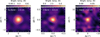 |
Fig. B.1 CI Tau Ku, X, and C band images, the first one reconstructed with uniform weighting and the others with natural weighting. Disc emission is unresolved at all the wavelengths. Grey contours indicate the 3σ, 5σ, 10σ (for Ku band data), and 15σ (for X band data) detection levels. |
Appendix C frank visibility fits
For ALMA data we first (re-)computed and set the weights based on the variance of the data using the CASA task statwt. This step had no visible effect on the images and radial profiles reconstructed using tclean, but significantly improved the residual maps of our visibility fits, especially in the case of band 3 data. CI Tau visibilities were then extracted from each dataset after applying time averaging to 30 and 60 s (for ALMA and VLA Ka bands, respectively), and spectral averaging to one channel per SPW16. First, we determined the disc offset from the phase centre (Δα, Δδ), fitting a Gaussian, whose inclination and position angle were fixed to the best-fit values of Clarke et al. (2018), to the visibility. Compared to a full fit of the disc geometry, this choice reduced the significance of large scale residuals (due to the PA being off by up to 4 deg in Band 3 and 30 deg in Ka band). The visibilities where then deprojected and inspected for the presence of flux density offsets. In the case of ALMA Band 3 and VLA Ka band data, where such offsets are clearly present, they were subtracted as discussed in Section C.1. Subsequently, the resulting visibilities where fitted in log-space, to avoid negative solutions and reduce non-physical wiggles, using the hyperparameters in Columns (2)–(5) of Table K.4. The deprojected visibilities, our best fits, and the residuals are shown in Figure C.1 and C.2, while the best-fit surface brightness profiles are plotted in purple in the central column of Figure 1. We measured the 68% and 95% flux radius from these profiles using a curve of growth method17. Size uncertainties were estimated as for the CLEAN image radial profiles, from the uncertainties obtained from the covariance matrix of the visibility fit (see Equation 28 of Junklewitz et al. 2016). Our results are summarised in Columns (6)–(7) of Table K.4. In the case of R68%, that is less sensitive to the profile cut-off, they confirm the trend already seen in the tclean profiles, of a decreasing disc size with wavelength. Except for VLA Ka band data, where the frank profiles clearly detect extended emission up to ≲ ![Mathematical equation: $\[1^{\prime\prime}_\cdot5\]$](/articles/aa/full_html/2025/10/aa52986-24/aa52986-24-eq66.png) , and due to the point-source subtraction, the dust sizes agree well with those in Table K.3.
, and due to the point-source subtraction, the dust sizes agree well with those in Table K.3.
C.1 Point-source subtraction
The ALMA Band 3 and VLA Ka band deprojected visibilities display a clear flux density offset (i.e. on average are non-null at their longest baselines). Since a point source (PS) in the image plane maps to a constant in the Fourier space, we interpreted this offset as the contribution of a point-like source at the disc centre (e.g. due to free-free from the central star, or a localised, non-resolved inner disc wind, or gyrosynchrotron emission, see Section 3.2 for a discussion). Especially in the case of VLA data, where it accounts for about 50% of the emission, this flux density offset induces high-amplitude spurious oscillations in the fitted profile (e.g. Jennings et al. 2022a; Sierra et al. 2024). For this reason, we subtracted it from the deprojected visibilities and only considered the PS-subtracted visibilities in our frank fits.
We estimated the PS flux density by fitting a constant to the real part of the unbinned deprojected visibilities at the longest baselines. It goes without saying that our estimated PS flux density is considerably affected by the choice of the longest baseline we fit beyond of. In this paper, this is defined as the minimum baseline where the visibilities flatten out and determined as follows. First, we used the Levenberg-Marquardt algorithm implemented in scipy.optimize.curve_fit (Virtanen et al. 2020) to fit a linear function to the real part of the unbinned deprojected visibilities over a range of baselines q ∈ [q0, q0 + qincr], where q0, the minimum baseline, and qincr, the baseline width, are varied as follows. We chose 1.0 Mλ ≤ q0 ≤ 4.0 Mλ (3.0 for VLA Ka band data), progressively increasing by 0.1 Mλ, and for each q0 we varied 0.4 Mλ ≤ qincr ≤ 1.0 Mλ, every 0.1 Mλ. Then, for each chosen baseline width, we inspected the best-fit angular incline as a function of q0 and identified the minimum baseline that minimises the incline. Since, in principle, this can change as a function of the baseline width, we selected as the longest baseline to fit beyond of that consistently minimising the incline over most values of qincr. Then we used the Levenberg-Marquardt algorithm implemented in scipy.optimize.curve_fit to determine the PS flux density. These PS flux densities are displayed as dashed lines in both panels of Figure C.2.
In the case of ALMA Band 3 data, the minimum angular incline is attained for 2.0 ≤ q0/Mλ ≤ 2.4 regardless of qincr. For these values of q0, the PS flux density is 0.23 ± 0.03 mJy. For shorter minimum baselines, the angular incline rapidly increase, while for longer ones, it considerably depends on qincr and the PS flux density is highly uncertain. In the case of VLA Ka band data, instead, the picture is less clear because of the lower S/N. On the one hand, as can be seen in the bottom panel of Figure C.2, the visibilities locally peak between 1.0 and 1.6 Mλ, driving the PS flux density fictitiously up. On the other hand, as in the case of Band 3, at longer minimum baselines the PS flux rapidly becomes very uncertain. Thus, we chose 1.7 Mλ as longest baseline to fit beyond of, leading to a PS flux density of 0.16 ± 0.01 mJy. For this value of q0 the minimum angular incline is also roughly null.
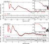 |
Fig. C.1 ALMA Band 7 (top) and 6 (bottom) deprojected (real part of the) visibilities, frank fits (red), and residuals. Data and residuals are averaged into bins of equal size (10−2 and 10−1 Mλ for grey and black dots, respectively). The inserts show the full visibility range. |
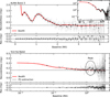 |
Fig. C.2 ALMA Band 3 (top) and VLA Ka band (bottom) deprojected (real part of the) visibilities, frank fits (red), and residuals. Data and residuals are averaged into bins of equal size (10−2 and 10−1 Mλ for grey and black dots, respectively). The dashed lines display the non-null flux density offset. The insert shows the full Band 3 visibility range. We plot the VLA Ka band visibilities in log-scale to highlight that emission is extended. |
Appendix D Radio emission variability
To explore the short-term continuum emission variability in the Ku and X band observations, we split our data scan by scan and measured their flux densities. Ku band data were taken two weeks apart (on February 19 and March 04, 2020), in 3 scans ≈7 min-long for each execution block, while X band data were taken the same day (August 03, 2019), in 12 scans ≈7 min-long. For both Ku and X band data, for each single-epoch dataset, we reconstructed continuum emission images and estimated their noise using the same parameters as in Appendix B, natural weighting, and a fixed circular mask of ![Mathematical equation: $\[5^{\prime\prime}_\cdot0\]$](/articles/aa/full_html/2025/10/aa52986-24/aa52986-24-eq67.png) and
and ![Mathematical equation: $\[1^{\prime\prime}_\cdot0\]$](/articles/aa/full_html/2025/10/aa52986-24/aa52986-24-eq68.png) radius for Ku and X band data, respectively (almost identical to those generated by auto-masking in Appendix B). Emission was detected in all the images with peak S/N > 20 for Ku band data and ≳ 3 for X band data. Since those detection levels are rather low, especially in X band, we opted to measure flux densities fitting the continuum visibilities for each single-epoch dataset with a PS model adopting a Bayesian approach similar to the one described in Section 4.2.
radius for Ku and X band data, respectively (almost identical to those generated by auto-masking in Appendix B). Emission was detected in all the images with peak S/N > 20 for Ku band data and ≳ 3 for X band data. Since those detection levels are rather low, especially in X band, we opted to measure flux densities fitting the continuum visibilities for each single-epoch dataset with a PS model adopting a Bayesian approach similar to the one described in Section 4.2.
Figure D.1 displays the time variability of the VLA Ku and X band emission, estimated as 100 × (1 − Fscan/Fconc), where Fscan is the flux density of each single-scan dataset and Fconc is the flux density of the concatenated dataset, measured in the visibility plane as for each scan. These flux densities are consistent, with those inferred by integrating the peak intensity of each tclean image over a synthesised beam within their 1σ RMS noise. The uncertainties were propagated from the confidence interval of each fit and, for Ku band single-epoch data, a 5% flux calibration uncertainty was also considered because observations were taken in different execution blocks. As is clear from Figure D.1, while the continuum flux density changes by ≲ 30% over a timescale of minutes to weeks in the Ku band, in the X band it dims by more than 50%, almost flares back in ≈15 min, and then remains steady in the subsequent hour. No emission is detected in the last scan.
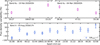 |
Fig. D.1 CI Tau VLA Ku (top) and X band (bottom) flux density variability is ≲ 30% over a timescale of minutes to hours (X band) and weeks (Ku band). |
Appendix E Temperature prior
In this Section we discuss the temperature prior used in our fit. For a passively irradiated disc, the mid-plane temperature profile can be approximated as (Kenyon & Hartmann 1987)
![Mathematical equation: $\[T=\left(\frac{\phi L_{\star}}{8 \pi R^2 \sigma_{\mathrm{SB}}}\right)^{1 / 4},\]$](/articles/aa/full_html/2025/10/aa52986-24/aa52986-24-eq69.png) (E.1)
(E.1)
where ϕ is the disc flaring angle, L⋆ is the stellar luminosity, R is the disc radius and σSB is the Stefan-Boltzmann constant. Following Macías et al. (2021), we assumed that the stellar luminosity is distributed as a Gaussian, with mean L⋆ = 1.04 L⊙18 and standard deviation 0.48L⊙ (Gangi et al. 2022), and that the flaring angle is uniformly distributed between 0.01 and 0.06.
We computed analytically the probability density function associated with the disc temperature considering the more general case of a random variable Z = (cXY)k, i.e. the power-law of the product of two random variables and a constant. The probability density function of this random variable can be written as
![Mathematical equation: $\[\begin{gathered}F_Z(z):=\mathbb{P}(Z \leq z)=\mathbb{P}\left((c X Y)^k \leq z\right)=\mathbb{P}\left(X Y \leq z^{1 / k} / c\right)= \\=\mathbb{P}\left(Y \leq z^{1 / k} / X c, X \geq 0\right)+\mathbb{P}\left(Y \geq z^{1 / k} / X c, X \leq 0\right)= \\=\int_0^{\infty} f_X(x) \int_{-\infty}^{z^{1 / k} / x c} f_Y(y) d y d x+ \\\qquad\qquad\qquad\qquad+\int_{-\infty}^0 f_X(x) \int_{z^{1 / k} / x c}^{\infty} f_Y(y) d y d x\end{gathered}\]$](/articles/aa/full_html/2025/10/aa52986-24/aa52986-24-eq70.png) (E.2)
(E.2)
by the fundamental theorem of calculus and the Leibniz rule
![Mathematical equation: $\[f_Z(z):=\frac{d}{d z} F_Z(z)=\int_{-\infty}^{\infty} f_X(x) f_Y\left(\frac{z^{1 / k}}{c x}\right) \frac{z^{1 / k-1}}{k c|x|} d x.\]$](/articles/aa/full_html/2025/10/aa52986-24/aa52986-24-eq71.png) (E.3)
(E.3)
If we take X to be distributed as a Gaussian with mean μ and standard deviation σ, and Y to be uniformly distributed between ymin and ymax, then
![Mathematical equation: $\[\begin{aligned}f_Z(z)= & \frac{1}{y_{\max }}-y_{\min } \frac{1}{\sqrt{2 \pi \sigma^2}} \times \\&\quad \times \int_{z^{1 / k} / c y_{\max }}^{z^{1 / k} / c y_{\min }} \exp \left\{-\frac{(x-\mu)^2}{2 \sigma^2}\right\} \frac{z^{1 / k-1}}{k c x} d x.\end{aligned}\]$](/articles/aa/full_html/2025/10/aa52986-24/aa52986-24-eq72.png) (E.4)
(E.4)
When z = T, x = L*, y = ϕ, c = (8πR2σSB)−1 and k = 0.25, Equation E.4 gives the probability density function corresponding to our definition of the temperature profile in Equation E.1.
Appendix F Data and model comparison
As a sanity-check, in this section we show that the posterior distribution of our fitting parameters can recover the input surface brightness and spectral index radial profiles. To do so, we used our MCMC samples to determine the posterior distributions of the model intensity, Sν, at 0.9, 1.3, 3.1, and 9.1 mm, and the spectral indices (αB7–B6, αB6–B3, and αB3–Ka), radius by radius.
Figure F.1 displays the azimuthally averaged ALMA Band 7, 6,3 (![Mathematical equation: $\[0^{\prime\prime}_\cdot058\]$](/articles/aa/full_html/2025/10/aa52986-24/aa52986-24-eq73.png) resolution) and VLA Ka band (
resolution) and VLA Ka band (![Mathematical equation: $\[0^{\prime\prime}_\cdot195\]$](/articles/aa/full_html/2025/10/aa52986-24/aa52986-24-eq74.png) resolution) surface brightness radial profiles as purple solid lines and their uncertainty (the quadrature sum of the error of the mean due to deprojection and the absolute flux density calibration uncertainty) as a shaded region of the same colour. The median and 1σ spread of our (high resolution for ALMA bands and low resolution for VLA Ka band) model (defined as the region between the 16th and 84th percentiles of the posterior distribution) surface brightness radial profiles are shown as black dashed lines and shaded areas of the same colour. A remarkable agreement can be seen between the data and model profiles at all the wavelengths.
resolution) surface brightness radial profiles as purple solid lines and their uncertainty (the quadrature sum of the error of the mean due to deprojection and the absolute flux density calibration uncertainty) as a shaded region of the same colour. The median and 1σ spread of our (high resolution for ALMA bands and low resolution for VLA Ka band) model (defined as the region between the 16th and 84th percentiles of the posterior distribution) surface brightness radial profiles are shown as black dashed lines and shaded areas of the same colour. A remarkable agreement can be seen between the data and model profiles at all the wavelengths.
Similarly, Figure F.2 displays the spectral index radial profiles extracted as is Section 3.2 in violet (for αB7–B6), purple (for αB6–B3), and yellow (for αB3–Ka). Their uncertainties were obtained propagating those on the azimuthally averaged surface brightness radial profiles and include the absolute flux density calibration error. The median and 1σ spread of our model spectral indices (defined as for the surface brightness radial profile posteriors above) are shown as black dashed lines and shaded areas of the same colour. Models and observations are in remarkable agreement, with the exception of the αB7–B6 profiles. This is because the model surface brightness radial profile slightly over-estimates (underestimates) the observed ALMA Band 6 (7) one by ≈10% (5%). Increasing the absolute flux calibration uncertainty does not improve the agreement between models and data.
To further investigate the origins of this discrepancy, we performed a low resolution fit with an additional free parameter: a brightness scale factor for the 1.3 mm data that can be interpreted as a flux calibration offset. We adopted this additional degree of freedom only for the ALMA Band 6 surface brightness radial profile because, as discussed in Appendix A, its flux calibration uncertainty is the largest among our data due to the light curve variability of the LB flux calibrator. Although, by construction, this scale factor is allowed to be different at each radius, its posterior distributions are similar at all the radii as long as the VLA Ka band surface brightness radial profile is detected with S/N > 5. In particular, its median is radially constant, and it perfectly matches the flux density offset between the two EBs of our Band 6 LB data (1.128). This suggests that LB0 (rather than LB1; see Appendix A) should be used as a reference EB when setting the Band 6 LB flux scale. This conclusion is also in line with the recently published SMA photometry of CI Tau (Chung et al. 2024). We also re-ran our fitting procedure after re-scaling our Band 6 surface brightness radial profile by the flux density offset determined in the previous step. Our results show that, in this case, the quality of the fit improves and the mismatch between αB7–B6 and our models completely vanishes. The marginalised posterior distributions of the four fitted parameters are perfectly consistent with those shown in Figure 4.
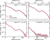 |
Fig. F.1 Comparison between the azimuthally averaged ALMA Band 7, 6, 3, and VLA Ka band surface brightness radial profiles (purple solid line and shaded region, including the calibration uncertainty) with the posterior distribution of our fit (black dashed line and shaded region, for the median and the area between the 16th and 84th percentiles). Results from the high (low) resolution fit are displayed for ALMA (VLA) data. An excellent agreement between models and observations can be seen. |
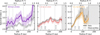 |
Fig. F.2 Same as in Figure F.1, but for the spectral index radial profiles discussed in Section 3.3 (see Figure 3). Results from the high (low) resolution fit are displayed for αB7–B6 and αB6–B3 (αB3–Ka) data. |
Appendix G Best-fit radial profiles
For the three sets of compositions (‘Ricci (compact)’, ‘Zubko (BE)’, and ‘DSHARP (default)’) that provide the best agreement with our data, we also performed high angular resolution fits19 as explained in Section 4.3. Corner plots comparing the posterior distributions obtained for such opacities at the position of the three bright rings in the system can be found in Appendix J, while their marginalised posterior distributions are displayed in Figure G.1 in blue, turquoise, and yellow, respectively.
As is clear from the upper-left panel, the temperature profile is consistent with that of a passively irradiated disc regardless of the assumed dust composition. Instead, the marginalised posteriors for the other fitting parameters show substantial differences. The dust surface density profiles, displayed in the upper-right panel of Figure G.1, all decrease towards the outer disc and locally peak at the position of the bright rings. However, while the posterior distributions obtained for ‘Ricci (compact)’ and ‘Zubko (BE)’ opacities are very similar (within less than a factor of two), the ‘DSHARP (default)’ composition prefers a much denser disc (more than a factor of six, increasing up to fifteen in the inner disc). This discrepancy is due to the different absorption opacity normalisation among these sets of optical properties (and more specifically the different dielectric constants of amorphous carbon and refractory organics), as can be seen in the left panel of Figure G.2, clearly showing that the ‘DSHARP (default)’ mixture is the less absorbing one among those tested. Moving on to the bottom-left panel of Figure G.1, the ‘Ricci (compact)’ and ‘Zubko (BE)’ mixtures also lead to similarly flat maximum grain size radial profiles with comparable magnitudes (amax ≈ 7.4 × 10⁻² cm and 2.9 × 10⁻² cm, respectively). Instead, the best-fit profile obtained for the ‘DSHARP (default)’ opacities is not flat, but peaks at the location of the outermost dust gap. We do not consider this feature to be physical, but more likely an artefact of the low S/N of our VLA Ka band data at these locations, combined with the lower flexibility of the optical properties of this mixture. The ‘DSHARP (default)’ opacities also favour the presence of much larger grains in this system, with amax ≈ 2.5 × 10⁻¹ cm (i.e. more than three times larger than for ‘Ricci (compact)’ grains). This discrepancy is primarily due to the different location of the Mie resonance in the βabs profile for the optical properties we considered (see the right panel of Figure G.2). Finally, as can be seen from the bottom-right panel of Figure G.1, the ‘Ricci (compact)’ and ‘Zubko (BE)’ opacities display similar trends in the dust density distribution too. Noticeably, in the outer disc these profiles are also in line with those inferred adopting the ‘DSHARP (default)’ composition. However, in this case the density distribution sharply decreases and flattens to q ≈ 1.5 for R ≤ 100 au. Once again, this behaviour can be motivated by the significantly higher minimum absorption spectral index (for any fixed dust density distribution) for the ‘DSHARP (default)’ mixture compared with the ‘Ricci (compact)’ and ‘Zubko (BE)’ ones, as can be seen in the right panel of Figure G.2 for amax ≳ 1 mm. Thus, since for steeper dust density distributions the Mie resonance is sharper, the only possibility of fitting both the large αB3–Ka and the small αB6–B3 with ‘DSHARP (default)’ grains is to prefer a smaller q. Instead, the sharp transition between the inner and the outer disc is due to the increase in αB6–B3 and the lower VLA Ka band S/N, that makes αB3–Ka more easy to fit because of its larger uncertainty.
Our results for the three dust compositions considered in this section agree that CI Tau’s continuum emission is (marginally) optically thin between 0.9 and 9.1 mm, but their best-fit optical depths show remarkable differences. In fact, while for both the ‘Ricci (compact)’ and ‘Zubko (BE)’ mixtures τν ≤ 0.4 even at 0.9 mm, for the ‘DSHARP (default)’ composition we inferred significantly higher optical depths, with τν ≥ 0.1 already at 9.1 mm. This difference is primarily driven by the single-scattering albedo. Indeed, because of their higher absorption opacity (left panel of Figure G.2), for the mixtures including amorphous carbon (i.e. ‘Ricci (compact)’ and ‘Zubko (BE)’) ων ≤ 0.5. Instead, when the ‘DSHARP (default)’ composition is considered, our results suggest that ων ≥ 0.6 (and ων ≥ 0.8 for λ ≥ 3.1 mm), leading to a more opaque disc. However, in the (marginally) optically thin limit, these two effects compensate each other: a higher optical depth increases continuum emission (second term in the curly brackets of Equation 2), but a larger albedo reduces it (third term in the curly brackets of Equation 2), and indeed, unsurprisingly, the absorption optical depth (i.e. ![Mathematical equation: $\[\tau_{\nu}^{\mathrm{abs}}=\Sigma_{\text {dust}} \kappa_{\nu}^{\mathrm{abs}}\]$](/articles/aa/full_html/2025/10/aa52986-24/aa52986-24-eq75.png) ), is, in fact, almost identical for the three compositions we tested (at each wavelength). As a final remark, we stress that these optical depth differences come as an additional opportunity to tell what dust mixtures can explain CI Tau’s observations the best, for example by comparison with an independent estimate of the total dust extinction. In this regard, a promising direction is the direct measurement of the line-of-sight dust extinction based on the attenuation of the CO brightness from the back side of the disc at the position of bright dust rings, as successfully demonstrated by Isella et al. (2018) for HD 163296 and Guzmán et al. (2018) for AS 209. Although comparable-quality CO observations are also available for CI Tau (Rosotti et al. 2021), they are significantly affected by cloud absorption, and emission from the back side of the disc is detected with too low S/N to perform a similar analysis.
), is, in fact, almost identical for the three compositions we tested (at each wavelength). As a final remark, we stress that these optical depth differences come as an additional opportunity to tell what dust mixtures can explain CI Tau’s observations the best, for example by comparison with an independent estimate of the total dust extinction. In this regard, a promising direction is the direct measurement of the line-of-sight dust extinction based on the attenuation of the CO brightness from the back side of the disc at the position of bright dust rings, as successfully demonstrated by Isella et al. (2018) for HD 163296 and Guzmán et al. (2018) for AS 209. Although comparable-quality CO observations are also available for CI Tau (Rosotti et al. 2021), they are significantly affected by cloud absorption, and emission from the back side of the disc is detected with too low S/N to perform a similar analysis.
To summarise, in addition to the larger χ2, already discussed in Section 5.3, the maximum grain size and dust density distribution profiles shown in Figure G.1 also provide clear indications (e.g. the aamax and q radial trends) that, compared with our fiducial ‘Ricci (compact)’ opacities, the ‘DSHARP (default)’ mixture gives less reliable results in the case of CI Tau. However, better data, such as deeper CO observations, are needed to confirm our statement. The ‘Ricci (compact)’ and both ‘Zubko’ mixtures, instead, fit our data better, converging to similar best-fit profiles. We are thus confident that the uncertainties on our results for Σdust and aamax displayed in Figure 4 are at most a factor of 3 and 2, respectively, when also considering different dust mixtures including amorphous carbonaceous grains.
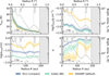 |
Fig. G.1 Same as in Figure 4 but showing a comparison among the best-fit results for different compositions: ‘Ricci (compact)’ in blue, ‘Zubko (BE)’ in turquoise, and ‘DSHARP (default)’ in yellow. The highest quality (i.e. lowest χ2) fits, obtained adopting the ‘Ricci (compact)’ and ‘Zubko (BE)’ optical properties, provide similar marginalised posterior distributions for all the parameters (within a factor of 3 for amax and 2 for Σdust). |
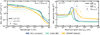 |
Fig. G.2 Left: Absorption opacity, |
![Mathematical equation: $\[\kappa_{\nu}^{\text{abs}}\]$](/articles/aa/full_html/2025/10/aa52986-24/aa52986-24-eq76.png)
![Mathematical equation: $\[\beta_{\text {B7}-\text {B3}}^{\text {abs}}\]$](/articles/aa/full_html/2025/10/aa52986-24/aa52986-24-eq77.png)
![Mathematical equation: $\[\beta_{\text {B3}-\text Ka }^{\text {abs}}\]$](/articles/aa/full_html/2025/10/aa52986-24/aa52986-24-eq78.png)
Appendix H Considerations on turbulence
In the scenario proposed by Jiang et al. (2024), the smooth maximum grain size radial profile inferred from our data can be interpreted as the consequence of turbulent fragmentation of fragile pebbles. Under the assumption of a standard (and homogeneous) dust-to-gas ratio, Z = 10−2, we can use our fiducial dust temperature, density, and grain size posterior distributions to estimate the (posterior probability of the) turbulence as a function of the disc radius in CI Tau as (see Equation 8 of Birnstiel et al. 2012)
![Mathematical equation: $\[\alpha_{\text {turb }}=\frac{2}{3 \pi} \frac{\Sigma_{\text {dust }}}{\rho_{\mathrm{s}} a_{\mathrm{max}}}\left(\frac{u_{\mathrm{frag}}}{c_{\mathrm{s}} Z}\right)^2,\]$](/articles/aa/full_html/2025/10/aa52986-24/aa52986-24-eq79.png) (H.1)
(H.1)
where ρs is the dust material density (1.70 g cm−3 for our fiducial ‘Ricci (compact)’ composition), ufrag is the fragmentation velocity threshold (1 × 102 cm s−1 for fragile pebbles, see the discussion of Pinilla et al. 2021 and Jiang et al. 2024, and the references therein), and ![Mathematical equation: $\[c_{\mathrm{s}} \propto T_{\text {dust}}^{1 / 2}\]$](/articles/aa/full_html/2025/10/aa52986-24/aa52986-24-eq80.png) is the locally isothermal sound speed.
is the locally isothermal sound speed.
Figure H.1 displays the posterior distribution of the turbulence radial profile for our fiducial “Ricci (compact)” dust mixture. This profile is approximately radially constant owing to the shallow dependence of the dust surface density on the disc radius (see Figure 4) and shows only low amplitude modulations at the location of the substructures in the continuum. Its magnitude (αturb ≈ 7.5 × 10⁻⁵) is comparable with that obtained under the same assumptions by Jiang et al. (2024) in TW Hya, AS 209, HD 163296, and GM Aur (in this latter case, the turbulence radial profile is also qualitatively similar to CI Tau’s one).
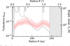 |
Fig. H.1 The pink solid lines and shaded regions display the median and 1σ uncertainty of the turbulence radial profile estimated for our fiducial “Ricci (compact)” composition. For comparison, the dotted lines show the results of the low resolution fit. |
Appendix I Absorption spectral index
Figure I.1 displays the posterior distribution of the absorption spectral index (βabs) radial profile between ALMA Band 7 and 3 (left), and ALMA Band 3 and VLA Ka band (right) for our fiducial “Ricci (compact)” composition in lilac. The absorption spectral index inferred from the spectral index radial profiles at the same wavelengths (Figure 3) in the optically thin assumption and Rayleigh-Jeans approximation (i.e. βabs = α − 2) is also plotted for comparison. In both panels, the two profiles show almost identical radial trends (e.g. both ![Mathematical equation: $\[\beta_{\mathrm{B} 7-\mathrm{B} 3}^{\mathrm{abs}}\]$](/articles/aa/full_html/2025/10/aa52986-24/aa52986-24-eq81.png) and αB7–B3 − 2 peak at the position of the dark rings in the continuum) with little offsets, that can be explained as follows. The marginal optical depth of our ALMA Band 7 and 3 data in the inner disc, and the low best-fit temperature (Tdust < 20 K) in the outer disc, impose corrections to the assumption that dust emission is completely optically thin and in the Rayleigh-Jeans approximation for
and αB7–B3 − 2 peak at the position of the dark rings in the continuum) with little offsets, that can be explained as follows. The marginal optical depth of our ALMA Band 7 and 3 data in the inner disc, and the low best-fit temperature (Tdust < 20 K) in the outer disc, impose corrections to the assumption that dust emission is completely optically thin and in the Rayleigh-Jeans approximation for ![Mathematical equation: $\[\beta_{\mathrm{B} 7-\mathrm{B} 3}^{\mathrm{abs}}\]$](/articles/aa/full_html/2025/10/aa52986-24/aa52986-24-eq82.png) . Instead, the discrepancies between
. Instead, the discrepancies between ![Mathematical equation: $\[\beta_{\mathrm{B} 3-\mathrm{Ka}}^{\mathrm{abs}}\]$](/articles/aa/full_html/2025/10/aa52986-24/aa52986-24-eq83.png) and αB3–Ka − 2 are mostly due to our fit preference for a fainter VLA Ka band emission profile than the median azimuthal average (see comparison in Figure F.1). As a final remark, we stress that our
and αB3–Ka − 2 are mostly due to our fit preference for a fainter VLA Ka band emission profile than the median azimuthal average (see comparison in Figure F.1). As a final remark, we stress that our ![Mathematical equation: $\[\beta_{\mathrm{B} 7-\mathrm{B} 3}^{\mathrm{abs}}\]$](/articles/aa/full_html/2025/10/aa52986-24/aa52986-24-eq84.png) radial profile increases towards the outer disc. While this trend is qualitatively consistent with the results of Guilloteau et al. (2011), who analysed together IRAM PdBI 1.3 and 2.7 mm observations of CI Tau prescribing different functional forms for the absorption spectral index radial profile, it is, however, in contrast with the results of Tazzari et al. (2021), who interpreted the almost constant dust disc sizes between 0.9 and 3.1 mm of a sample of 26 bright discs in Lupus as the consequence of a radially constant
radial profile increases towards the outer disc. While this trend is qualitatively consistent with the results of Guilloteau et al. (2011), who analysed together IRAM PdBI 1.3 and 2.7 mm observations of CI Tau prescribing different functional forms for the absorption spectral index radial profile, it is, however, in contrast with the results of Tazzari et al. (2021), who interpreted the almost constant dust disc sizes between 0.9 and 3.1 mm of a sample of 26 bright discs in Lupus as the consequence of a radially constant ![Mathematical equation: $\[\beta_{\mathrm{B} 7-\mathrm{B} 3}^{\mathrm{abs}}\]$](/articles/aa/full_html/2025/10/aa52986-24/aa52986-24-eq85.png) radial profile. This difference suggests that, rather than a flat absorption spectral index, outer disc substructures might the reason behind the nearly wavelength-invariant dust disc size at ALMA wavelengths inferred by Tazzari et al. (2021, see the case of CX Tau, that shows no substructured down to a
radial profile. This difference suggests that, rather than a flat absorption spectral index, outer disc substructures might the reason behind the nearly wavelength-invariant dust disc size at ALMA wavelengths inferred by Tazzari et al. (2021, see the case of CX Tau, that shows no substructured down to a ![Mathematical equation: $\[0^{\prime\prime}_\cdot040\]$](/articles/aa/full_html/2025/10/aa52986-24/aa52986-24-eq86.png) ≈ 5 au resolution, Facchini et al. 2019, and whose dust sizes decline with wavelength as predicted by radial drift models, Curone et al. 2023).
≈ 5 au resolution, Facchini et al. 2019, and whose dust sizes decline with wavelength as predicted by radial drift models, Curone et al. 2023).
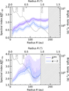 |
Fig. I.1 Absorption spectral index (βabs) posterior distributions for our fiducial “Ricci (compact)” composition in lilac and the spectral index (α − 2) radial profile in blue between ALMA Band 7 and 3 (left), and ALMA Band 3 and VLA Ka band (right). The solid lines and shaded regions display the median and 1σ uncertainty of each parameter. For comparison, the dotted lines show the results of the low resolution fit. |
Appendix J Corner plot comparisons
Figure J.1, J.2, and J.3 show a comparison of the posterior distributions of our high resolution fits for different assumptions on the dust optical properties: ‘Ricci (compact)’ in blue, ‘Zubko (BE)’ in turquoise, and ‘DSHARP (default)’ in yellow.
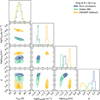 |
Fig. J.1 Comparison of the MCMC posteriors for different assumptions on dust optical properties at the position of the inner ring (R = 26.5 au). |
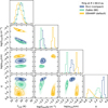 |
Fig. J.2 Same as in Figure J.1 at the position of the central ring (R = 60.0 au). |
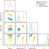 |
Fig. J.3 Same as in Figure J.1 and J.2 at the position of the outer ring (R = 151.1 au). |
Appendix K Tables
Summary of CI Tau’s stellar properties.
Summary of the new and archival datasets (re-)analysed in this paper.
Imaging results.
frank fit hyper-parameters and disc sizes.
Comparison between pebble masses measured in the optically thin approximation and from multi-frequency continuum observations for the best studied sources in the literature and CI Tau.
References
- Alcalá, J. M., Manara, C. F., Natta, A., et al. 2017, A&A, 600, A20 [NASA ADS] [CrossRef] [EDP Sciences] [Google Scholar]
- ALMA Partnership (Brogan, C. L., et al.) 2015, ApJ, 808, L3 [Google Scholar]
- Andrews, S. M. 2020, ARA&A, 58, 483 [Google Scholar]
- Andrews, S. M., & Williams, J. P. 2005, ApJ, 631, 1134 [Google Scholar]
- Andrews, S. M., & Williams, J. P. 2007, ApJ, 659, 705 [NASA ADS] [CrossRef] [Google Scholar]
- Andrews, S. M., Rosenfeld, K. A., Kraus, A. L., & Wilner, D. J. 2013, ApJ, 771, 129 [Google Scholar]
- Andrews, S. M., Wilner, D. J., Zhu, Z., et al. 2016, ApJ, 820, L40 [Google Scholar]
- Andrews, S. M., Huang, J., Pérez, L. M., et al. 2018, ApJ, 869, L41 [NASA ADS] [CrossRef] [Google Scholar]
- Andrews, S. M., Elder, W., Zhang, S., et al. 2021, ApJ, 916, 51 [NASA ADS] [CrossRef] [Google Scholar]
- Anglada, G., Rodríguez, L. F., & Carrasco-González, C. 2018, A&A Rev., 26, 3 [Google Scholar]
- Ansdell, M., Williams, J. P., van der Marel, N., et al. 2016, ApJ, 828, 46 [Google Scholar]
- Ansdell, M., Williams, J. P., Trapman, L., et al. 2018, ApJ, 859, 21 [NASA ADS] [CrossRef] [Google Scholar]
- Astropy Collaboration (Robitaille, T. P., et al.) 2013, A&A, 558, A33 [NASA ADS] [CrossRef] [EDP Sciences] [Google Scholar]
- Astropy Collaboration (Price-Whelan, A. M., et al.) 2018, AJ, 156, 123 [Google Scholar]
- Astropy Collaboration (Price-Whelan, A. M., et al.) 2022, ApJ, 935, 167 [NASA ADS] [CrossRef] [Google Scholar]
- Bacciotti, F., Girart, J. M., Padovani, M., et al. 2018, ApJ, 865, L12 [Google Scholar]
- Bae, J., Isella, A., Zhu, Z., et al. 2023, in Astronomical Society of the Pacific Conference Series, 534, Protostars and Planets VII, eds. S. Inutsuka, Y. Aikawa, T. Muto, K. Tomida, & M. Tamura, 423 [Google Scholar]
- Banzatti, A., Testi, L., Isella, A., et al. 2011, A&A, 525, A12 [NASA ADS] [CrossRef] [EDP Sciences] [Google Scholar]
- Barenfeld, S. A., Carpenter, J. M., Ricci, L., & Isella, A. 2016, ApJ, 827, 142 [Google Scholar]
- Beckwith, S. V. W., & Sargent, A. I. 1991, ApJ, 381, 250 [NASA ADS] [CrossRef] [Google Scholar]
- Beckwith, S. V. W., Sargent, A. I., Chini, R. S., & Guesten, R. 1990, AJ, 99, 924 [Google Scholar]
- Beitz, E., Güttler, C., Blum, J., et al. 2011, ApJ, 736, 34 [NASA ADS] [CrossRef] [Google Scholar]
- Bergner, J. B., Öberg, K. I., Bergin, E. A., et al. 2019, ApJ, 876, 25 [Google Scholar]
- Biddle, L. I., Johns-Krull, C. M., Llama, J., Prato, L., & Skiff, B. A. 2018, ApJ, 853, L34 [NASA ADS] [CrossRef] [Google Scholar]
- Biddle, L. I., Llama, J., Cameron, A., et al. 2021, ApJ, 906, 113 [NASA ADS] [CrossRef] [Google Scholar]
- Birnstiel, T. 2024, ARA&A, 62, 157 [NASA ADS] [CrossRef] [Google Scholar]
- Birnstiel, T., & Andrews, S. M. 2014, ApJ, 780, 153 [Google Scholar]
- Birnstiel, T., Dullemond, C. P., & Brauer, F. 2010, A&A, 513, A79 [NASA ADS] [CrossRef] [EDP Sciences] [Google Scholar]
- Birnstiel, T., Ormel, C. W., & Dullemond, C. P. 2011, A&A, 525, A11 [NASA ADS] [CrossRef] [EDP Sciences] [Google Scholar]
- Birnstiel, T., Klahr, H., & Ercolano, B. 2012, A&A, 539, A148 [NASA ADS] [CrossRef] [EDP Sciences] [Google Scholar]
- Birnstiel, T., Dullemond, C. P., Zhu, Z., et al. 2018, ApJ, 869, L45 [CrossRef] [Google Scholar]
- Bohren, C. F., & Huffman, D. R. 1998, Absorption and Scattering of Light by Small Particles [Google Scholar]
- Booth, R. A., & Ilee, J. D. 2019, MNRAS, 487, 3998 [CrossRef] [Google Scholar]
- Booth, R. A., Clarke, C. J., Madhusudhan, N., & Ilee, J. D. 2017, MNRAS, 469, 3994 [Google Scholar]
- Brauer, F., Dullemond, C. P., & Henning, T. 2008, A&A, 480, 859 [NASA ADS] [CrossRef] [EDP Sciences] [Google Scholar]
- Bridle, A. H., & Schwab, F. R. 1989, in Astronomical Society of the Pacific Conference Series, 6, Synthesis Imaging in Radio Astronomy, eds. R. A. Perley, F. R. Schwab, & A. H. Bridle, 247 [Google Scholar]
- Briggs, D. S. 1995, PhD thesis, New Mexico Institute of Mining and Technology [Google Scholar]
- Bruggeman, D. A. G. 1935, Ann. Phys., 416, 636 [Google Scholar]
- Carrasco-González, C., Sierra, A., Flock, M., et al. 2019, ApJ, 883, 71 [Google Scholar]
- Carrera, D., Simon, J. B., Li, R., Kretke, K. A., & Klahr, H. 2021, AJ, 161, 96 [Google Scholar]
- Carrera, D., Thomas, A. J., Simon, J. B., et al. 2022, ApJ, 927, 52 [NASA ADS] [CrossRef] [Google Scholar]
- Carvalho, A. S., Pérez, L. M., Sierra, A., et al. 2024, ApJ, 971, 129 [Google Scholar]
- CASA Team (Bean, B., et al.) 2022, PASP, 134, 114501 [NASA ADS] [CrossRef] [Google Scholar]
- Chung, C.-Y., Andrews, S. M., Gurwell, M. A., et al. 2024, ApJS, 273, 29 [NASA ADS] [CrossRef] [Google Scholar]
- Chung, C.-Y., Tsai, A.-L., Wright, M., et al. 2025, ApJS, 277, 45 [Google Scholar]
- Clarke, C. J., Tazzari, M., Juhasz, A., et al. 2018, ApJ, 866, L6 [NASA ADS] [CrossRef] [Google Scholar]
- Cornwell, T. J. 2008, IEEE J. Selected Top. Signal Process., 2, 793 [NASA ADS] [CrossRef] [Google Scholar]
- Coutens, A., Liu, H. B., Jiménez-Serra, I., et al. 2019, A&A, 631, A58 [NASA ADS] [CrossRef] [EDP Sciences] [Google Scholar]
- Cuello, N., Ménard, F., & Price, D. J. 2023, Eur. Phys. J. Plus, 138, 11 [NASA ADS] [CrossRef] [Google Scholar]
- Curone, P., Testi, L., Macías, E., et al. 2023, A&A, 677, A118 [NASA ADS] [CrossRef] [EDP Sciences] [Google Scholar]
- Czekala, I., Loomis, R. A., Teague, R., et al. 2021, ApJS, 257, 2 [NASA ADS] [CrossRef] [Google Scholar]
- Delussu, L., Birnstiel, T., Miotello, A., et al. 2024, A&A, 688, A81 [NASA ADS] [CrossRef] [EDP Sciences] [Google Scholar]
- Dent, W. R. F., Pinte, C., Cortes, P. C., et al. 2019, MNRAS, 482, L29 [Google Scholar]
- Desch, S. J., & Turner, N. J. 2015, ApJ, 811, 156 [NASA ADS] [CrossRef] [Google Scholar]
- Doi, K., & Kataoka, A. 2023, ApJ, 957, 11 [CrossRef] [Google Scholar]
- Dominik, C., & Dullemond, C. P. 2024, A&A, 682, A144 [NASA ADS] [CrossRef] [EDP Sciences] [Google Scholar]
- Dominik, C., Min, M., & Tazaki, R. 2021, OpTool: Command-line driven tool for creating complex dust opacities, Astrophysics Source Code Library [record ascl:2104.010] [Google Scholar]
- Donati, J. F., Bouvier, J., Alencar, S. H., et al. 2020, MNRAS, 491, 5660 [Google Scholar]
- Donati, J. F., Finociety, B., Cristofari, P. I., et al. 2024, MNRAS, 530, 264 [NASA ADS] [CrossRef] [Google Scholar]
- Dong, R., Liu, S.-y., Eisner, J., et al. 2018, ApJ, 860, 124 [Google Scholar]
- Dorschner, J., Begemann, B., Henning, T., Jaeger, C., & Mutschke, H. 1995, A&A, 300, 503 [Google Scholar]
- Draine, B. T. 2003, ARA&A, 41, 241 [NASA ADS] [CrossRef] [Google Scholar]
- Drążkowska, J., Bitsch, B., Lambrechts, M., et al. 2023, in Astronomical Society of the Pacific Conference Series, 534, Protostars and Planets VII, eds. S. Inutsuka, Y. Aikawa, T. Muto, K. Tomida, & M. Tamura, 717 [Google Scholar]
- Dulk, G. A. 1985, ARA&A, 23, 169 [Google Scholar]
- Dulk, G. A., & Marsh, K. A. 1982, ApJ, 259, 350 [NASA ADS] [CrossRef] [Google Scholar]
- Dullemond, C. P., Birnstiel, T., Huang, J., et al. 2018, ApJ, 869, L46 [NASA ADS] [CrossRef] [Google Scholar]
- Dutrey, A., Guilloteau, S., Duvert, G., et al. 1996, A&A, 309, 493 [NASA ADS] [Google Scholar]
- Dzib, S. A., Loinard, L., Mioduszewski, A. J., et al. 2013, ApJ, 775, 63 [Google Scholar]
- Dzib, S. A., Loinard, L., Rodríguez, L. F., et al. 2015, ApJ, 801, 91 [Google Scholar]
- Facchini, S., Birnstiel, T., Bruderer, S., & van Dishoeck, E. F. 2017, A&A, 605, A16 [NASA ADS] [CrossRef] [EDP Sciences] [Google Scholar]
- Facchini, S., van Dishoeck, E. F., Manara, C. F., et al. 2019, A&A, 626, L2 [NASA ADS] [CrossRef] [EDP Sciences] [Google Scholar]
- Facchini, S., Benisty, M., Bae, J., et al. 2020, A&A, 639, A121 [EDP Sciences] [Google Scholar]
- Fairlamb, J. R., Oudmaijer, R. D., Mendigutía, I., Ilee, J. D., & van den Ancker, M. E. 2015, MNRAS, 453, 976 [Google Scholar]
- Flagg, L., Johns-Krull, C. M., Nofi, L., et al. 2019, ApJ, 878, L37 [NASA ADS] [CrossRef] [Google Scholar]
- Foreman-Mackey, D. 2016, J. Open Source Softw., 1, 24 [Google Scholar]
- Foreman-Mackey, D., Hogg, D. W., Lang, D., & Goodman, J. 2013, PASP, 125, 306 [Google Scholar]
- Foreman-Mackey, D., Farr, W., Sinha, M., et al. 2019, J. Open Source Softw., 4, 1864 [NASA ADS] [CrossRef] [Google Scholar]
- Gaia Collaboration 2020, VizieR Online Data Catalog: I/350 [Google Scholar]
- Gaia Collaboration (Vallenari, A., et al.) 2023, A&A, 674, A1 [NASA ADS] [CrossRef] [EDP Sciences] [Google Scholar]
- Galli, P. A. B., Loinard, L., Ortiz-Léon, G. N., et al. 2018, ApJ, 859, 33 [Google Scholar]
- Gangi, M., Antoniucci, S., Biazzo, K., et al. 2022, A&A, 667, A124 [NASA ADS] [CrossRef] [EDP Sciences] [Google Scholar]
- Garufi, A., Dominik, C., Ginski, C., et al. 2022, A&A, 658, A137 [NASA ADS] [CrossRef] [EDP Sciences] [Google Scholar]
- Gavino, S., Dutrey, A., Wakelam, V., et al. 2021, A&A, 654, A65 [NASA ADS] [CrossRef] [EDP Sciences] [Google Scholar]
- Ginski, C., Tazaki, R., Dominik, C., & Stolker, T. 2023, ApJ, 953, 92 [NASA ADS] [CrossRef] [Google Scholar]
- Goldreich, P., & Ward, W. R. 1973, ApJ, 183, 1051 [Google Scholar]
- Goodman, J., & Weare, J. 2010, Commun. Appl. Math. Computat. Sci., 5, 65 [Google Scholar]
- GRAVITY Collaboration (Soulain, A., et al.) 2023, A&A, 674, A203 [NASA ADS] [CrossRef] [EDP Sciences] [Google Scholar]
- Güdel, M. 2002, ARA&A, 40, 217 [Google Scholar]
- Guerra-Alvarado, O. M., Carrasco-González, C., Macías, E., et al. 2024, A&A, 686, A298 [NASA ADS] [CrossRef] [EDP Sciences] [Google Scholar]
- Guidi, G., Ruane, G., Williams, J. P., et al. 2018, MNRAS, 479, 1505 [Google Scholar]
- Guidi, G., Isella, A., Testi, L., et al. 2022, A&A, 664, A137 [NASA ADS] [CrossRef] [EDP Sciences] [Google Scholar]
- Guillot, T., Fletcher, L. N., Helled, R., et al. 2023, in Astronomical Society of the Pacific Conference Series, 534, Protostars and Planets VII, eds. S. Inutsuka, Y. Aikawa, T. Muto, K. Tomida, & M. Tamura, 947 [Google Scholar]
- Guilloteau, S., Dutrey, A., Piétu, V., & Boehler, Y. 2011, A&A, 529, A105 [NASA ADS] [CrossRef] [EDP Sciences] [Google Scholar]
- Guzmán, V. V., Huang, J., Andrews, S. M., et al. 2018, ApJ, 869, L48 [Google Scholar]
- Haffert, S. Y., Bohn, A. J., de Boer, J., et al. 2019, Nat. Astron., 3, 749 [Google Scholar]
- Harris, C. R., Millman, K. J., van der Walt, S. J., et al. 2020, Nature, 585, 357 [NASA ADS] [CrossRef] [Google Scholar]
- Henning, T., & Stognienko, R. 1996, A&A, 311, 291 [NASA ADS] [Google Scholar]
- Henyey, L. G., & Greenstein, J. L. 1941, ApJ, 93, 70 [Google Scholar]
- Hildebrand, R. H. 1983, QJRAS, 24, 267 [NASA ADS] [Google Scholar]
- Hou, F., Goodman, J., & Hogg, D. W. 2014, arXiv e-prints [arXiv:1401.6128] [Google Scholar]
- Houge, A., Macías, E., & Krijt, S. 2024, MNRAS, 527, 9668 [Google Scholar]
- Huang, J., Andrews, S. M., Cleeves, L. I., et al. 2018a, ApJ, 852, 122 [Google Scholar]
- Huang, J., Andrews, S. M., Dullemond, C. P., et al. 2018b, ApJ, 869, L42 [NASA ADS] [CrossRef] [Google Scholar]
- Huang, J., Andrews, S. M., Pérez, L. M., et al. 2018c, ApJ, 869, L43 [Google Scholar]
- Huang, J., Andrews, S. M., Dullemond, C. P., et al. 2020a, ApJ, 891, 48 [Google Scholar]
- Huang, J., Andrews, S. M., Öberg, K. I., et al. 2020b, ApJ, 898, 140 [NASA ADS] [CrossRef] [Google Scholar]
- Hull, C. L. H., Yang, H., Li, Z.-Y., et al. 2018, ApJ, 860, 82 [Google Scholar]
- Hunter, J. D. 2007, Comput. Sci. Eng., 9, 90 [NASA ADS] [CrossRef] [Google Scholar]
- Hunter, T. R., Petry, D., Barkats, D., Corder, S., & Indebetouw, R. 2023, analysisUtils [Google Scholar]
- Isella, A., Carpenter, J. M., & Sargent, A. I. 2010, ApJ, 714, 1746 [Google Scholar]
- Isella, A., Huang, J., Andrews, S. M., et al. 2018, ApJ, 869, L49 [NASA ADS] [CrossRef] [Google Scholar]
- Jäger, C., Mutschke, H., & Henning, T. 1998, A&A, 332, 291 [NASA ADS] [Google Scholar]
- Jennings, J., Booth, R. A., Tazzari, M., Rosotti, G. P., & Clarke, C. J. 2020, MNRAS, 495, 3209 [Google Scholar]
- Jennings, J., Booth, R. A., Tazzari, M., Clarke, C. J., & Rosotti, G. P. 2022a, MNRAS, 509, 2780 [NASA ADS] [Google Scholar]
- Jennings, J., Tazzari, M., Clarke, C. J., Booth, R. A., & Rosotti, G. P. 2022b, MNRAS, 514, 6053 [NASA ADS] [CrossRef] [Google Scholar]
- Jiang, H., & Ormel, C. W. 2023, MNRAS, 518, 3877 [Google Scholar]
- Jiang, H., Macías, E., Guerra-Alvarado, O. M., & Carrasco-González, C. 2024, A&A, 682, A32 [NASA ADS] [CrossRef] [EDP Sciences] [Google Scholar]
- Johansen, A., Oishi, J. S., Mac Low, M.-M., et al. 2007, Nature, 448, 1022 [Google Scholar]
- Johns-Krull, C. M., McLane, J. N., Prato, L., et al. 2016, ApJ, 826, 206 [Google Scholar]
- Jorsater, S., & van Moorsel, G. A. 1995, AJ, 110, 2037 [Google Scholar]
- Junklewitz, H., Bell, M. R., Selig, M., & Enßlin, T. A. 2016, A&A, 586, A76 [NASA ADS] [CrossRef] [EDP Sciences] [Google Scholar]
- Kataoka, A., Okuzumi, S., Tanaka, H., & Nomura, H. 2014, A&A, 568, A42 [NASA ADS] [CrossRef] [EDP Sciences] [Google Scholar]
- Kataoka, A., Muto, T., Momose, M., et al. 2015, ApJ, 809, 78 [Google Scholar]
- Kataoka, A., Tsukagoshi, T., Momose, M., et al. 2016, ApJ, 831, L12 [Google Scholar]
- Kataoka, A., Tsukagoshi, T., Pohl, A., et al. 2017, ApJ, 844, L5 [Google Scholar]
- Kenyon, S. J., & Hartmann, L. 1987, ApJ, 323, 714 [Google Scholar]
- Kepley, A. A., Tsutsumi, T., Brogan, C. L., et al. 2020, PASP, 132, 024505 [Google Scholar]
- Keppler, M., Benisty, M., Müller, A., et al. 2018, A&A, 617, A44 [NASA ADS] [CrossRef] [EDP Sciences] [Google Scholar]
- Keppler, M., Teague, R., Bae, J., et al. 2019, A&A, 625, A118 [NASA ADS] [CrossRef] [EDP Sciences] [Google Scholar]
- Kirchschlager, F., & Bertrang, G. H. M. 2020, A&A, 638, A116 [NASA ADS] [CrossRef] [EDP Sciences] [Google Scholar]
- Kluyver, T., Ragan-Kelley, B., Pérez, F., et al. 2016, in Positioning and Power in Academic Publishing: Players, Agents and Agendas, eds. F. Loizides, & B. Schmidt (IOS Press), 87 [Google Scholar]
- Konishi, M., Hashimoto, J., & Hori, Y. 2018, ApJ, 859, L28 [CrossRef] [Google Scholar]
- Kozdon, J., Brittain, S. D., Fung, J., et al. 2023, AJ, 166, 119 [NASA ADS] [CrossRef] [Google Scholar]
- Krijt, S., Bosman, A. D., Zhang, K., et al. 2020, ApJ, 899, 134 [NASA ADS] [CrossRef] [Google Scholar]
- Kurtovic, N. T., Pérez, L. M., Benisty, M., et al. 2018, ApJ, 869, L44 [Google Scholar]
- Kwon, W., Looney, L. W., Mundy, L. G., & Welch, W. J. 2015, ApJ, 808, 102 [NASA ADS] [CrossRef] [Google Scholar]
- Lau, T. C. H., Drążkowska, J., Stammler, S. M., Birnstiel, T., & Dullemond, C. P. 2022, A&A, 668, A170 [NASA ADS] [CrossRef] [EDP Sciences] [Google Scholar]
- Law, C. J., Crystian, S., Teague, R., et al. 2022, ApJ, 932, 114 [NASA ADS] [CrossRef] [Google Scholar]
- Le Gal, R., Öberg, K. I., Loomis, R. A., Pegues, J., & Bergner, J. B. 2019, ApJ, 876, 72 [Google Scholar]
- Lesur, G., Flock, M., Ercolano, B., et al. 2023, in Astronomical Society of the Pacific Conference Series, 534, eds. S. Inutsuka, Y. Aikawa, T. Muto, K. Tomida, & M. Tamura, 465 [Google Scholar]
- Lin, Z.-Y. D., Li, Z.-Y., Yang, H., et al. 2020, MNRAS, 496, 169 [Google Scholar]
- Liu, H. B. 2019, ApJ, 877, L22 [NASA ADS] [CrossRef] [Google Scholar]
- Liu, H. B., Galván-Madrid, R., Forbrich, J., et al. 2014, ApJ, 780, 155 [Google Scholar]
- Lodato, G., Dipierro, G., Ragusa, E., et al. 2019, MNRAS, 486, 453 [Google Scholar]
- Lommen, D., Maddison, S. T., Wright, C. M., et al. 2009, A&A, 495, 869 [NASA ADS] [CrossRef] [EDP Sciences] [Google Scholar]
- Long, F., Pinilla, P., Herczeg, G. J., et al. 2018, ApJ, 869, 17 [Google Scholar]
- Lorek, S., Lacerda, P., & Blum, J. 2018, A&A, 611, A18 [NASA ADS] [CrossRef] [EDP Sciences] [Google Scholar]
- Macías, E., Anglada, G., Osorio, M., et al. 2016, ApJ, 829, 1 [Google Scholar]
- Macías, E., Espaillat, C. C., Osorio, M., et al. 2019, ApJ, 881, 159 [CrossRef] [Google Scholar]
- Macías, E., Guerra-Alvarado, O., Carrasco-González, C., et al. 2021, A&A, 648, A33 [EDP Sciences] [Google Scholar]
- Madhusudhan, N. 2019, ARA&A, 57, 617 [NASA ADS] [CrossRef] [Google Scholar]
- Manara, C. F., Morbidelli, A., & Guillot, T. 2018, A&A, 618, L3 [NASA ADS] [CrossRef] [EDP Sciences] [Google Scholar]
- Manick, R., Sousa, A. P., Bouvier, J., et al. 2024, A&A, 686, A249 [NASA ADS] [CrossRef] [EDP Sciences] [Google Scholar]
- Martire, P., Longarini, C., Lodato, G., et al. 2024, A&A, 686, A9 [Google Scholar]
- Mathis, J. S., Rumpl, W., & Nordsieck, K. H. 1977, ApJ, 217, 425 [Google Scholar]
- Maucó, K., Carrasco-González, C., Schreiber, M. R., et al. 2021, ApJ, 923, 128 [CrossRef] [Google Scholar]
- Maxwell Garnett, J. C. 1904, Philos. Trans. Roy. Soc. Lond. Ser. A, 203, 385 [NASA ADS] [CrossRef] [Google Scholar]
- McMullin, J. P., Waters, B., Schiebel, D., Young, W., & Golap, K. 2007, in Astronomical Society of the Pacific Conference Series, Vol. 376, Astronomical Data Analysis Software and Systems XVI, eds. R. A. Shaw, F. Hill, & D. J. Bell, 127 [Google Scholar]
- Menu, J., van Boekel, R., Henning, T., et al. 2014, A&A, 564, A93 [NASA ADS] [CrossRef] [EDP Sciences] [Google Scholar]
- Mezger, P. G., Schraml, J., & Terzian, Y. 1967, ApJ, 150, 807 [Google Scholar]
- Michoulier, S., Gonzalez, J.-F., & Price, D. J. 2024, A&A, 688, A31 [NASA ADS] [CrossRef] [EDP Sciences] [Google Scholar]
- Min, M., Rab, C., Woitke, P., Dominik, C., & Ménard, F. 2016, A&A, 585, A13 [NASA ADS] [CrossRef] [EDP Sciences] [Google Scholar]
- Miotello, A., Kamp, I., Birnstiel, T., Cleeves, L. C., & Kataoka, A. 2023, in Astronomical Society of the Pacific Conference Series, 534, Protostars and Planets VII, eds. S. Inutsuka, Y. Aikawa, T. Muto, K. Tomida, & M. Tamura, 501 [Google Scholar]
- Miyake, K., & Nakagawa, Y. 1993, Icarus, 106, 20 [NASA ADS] [CrossRef] [Google Scholar]
- Mulders, G. D., Pascucci, I., Ciesla, F. J., & Fernandes, R. B. 2021, ApJ, 920, 66 [NASA ADS] [CrossRef] [Google Scholar]
- Muley, D., & Dong, R. 2021, ApJ, 921, L34 [NASA ADS] [CrossRef] [Google Scholar]
- Najita, J. R., & Kenyon, S. J. 2014, MNRAS, 445, 3315 [NASA ADS] [CrossRef] [Google Scholar]
- Öberg, K. I., & Bergin, E. A. 2021, Phys. Rep., 893, 1 [Google Scholar]
- Öberg, K. I., Facchini, S., & Anderson, D. E. 2023, ARA&A, 61, 287 [CrossRef] [Google Scholar]
- Ohashi, S., Momose, M., Kataoka, A., et al. 2023, ApJ, 954, 110 [NASA ADS] [CrossRef] [Google Scholar]
- Okuzumi, S., Momose, M., Sirono, S.-i., Kobayashi, H., & Tanaka, H. 2016, ApJ, 821, 82 [Google Scholar]
- Olnon, F. M. 1975, A&A, 39, 217 [NASA ADS] [Google Scholar]
- Owen, J. E., Scaife, A. M. M., & Ercolano, B. 2013, MNRAS, 434, 3378 [CrossRef] [Google Scholar]
- Panagia, N., & Felli, M. 1975, A&A, 39, 1 [Google Scholar]
- Paneque-Carreño, T., Pérez, L. M., Benisty, M., et al. 2021, ApJ, 914, 88 [CrossRef] [Google Scholar]
- Pascucci, I., Gorti, U., & Hollenbach, D. 2012, ApJ, 751, L42 [Google Scholar]
- Pascucci, I., Testi, L., Herczeg, G. J., et al. 2016, ApJ, 831, 125 [Google Scholar]
- Pascucci, I., Cabrit, S., Edwards, S., et al. 2023, in Astronomical Society of the Pacific Conference Series, 534, Protostars and Planets VII, eds. S. Inutsuka, Y. Aikawa, T. Muto, K. Tomida, & M. Tamura, 567 [Google Scholar]
- Pérez, L. M., Carpenter, J. M., Chandler, C. J., et al. 2012, ApJ, 760, L17 [CrossRef] [Google Scholar]
- Pérez, L. M., Chandler, C. J., Isella, A., et al. 2015, ApJ, 813, 41 [CrossRef] [Google Scholar]
- Pérez, L. M., Carpenter, J. M., Andrews, S. M., et al. 2016, Science, 353, 1519 [Google Scholar]
- Pérez, L. M., Benisty, M., Andrews, S. M., et al. 2018, ApJ, 869, L50 [CrossRef] [Google Scholar]
- Petrovic, H. J., Booth, R. A., & Clarke, C. J. 2024, MNRAS [arXiv:2409.16245] [Google Scholar]
- Pinilla, P., Benisty, M., & Birnstiel, T. 2012, A&A, 545, A81 [NASA ADS] [CrossRef] [EDP Sciences] [Google Scholar]
- Pinilla, P., Lenz, C. T., & Stammler, S. M. 2021, A&A, 645, A70 [NASA ADS] [CrossRef] [EDP Sciences] [Google Scholar]
- Pinte, C., Dent, W. R. F., Ménard, F., et al. 2016, ApJ, 816, 25 [Google Scholar]
- Pollack, J. B., Hollenbach, D., Beckwith, S., et al. 1994, ApJ, 421, 615 [Google Scholar]
- Ragusa, E., Dipierro, G., Lodato, G., Laibe, G., & Price, D. J. 2017, MNRAS, 464, 1449 [Google Scholar]
- Ragusa, E., Rosotti, G., Teyssandier, J., et al. 2018, MNRAS, 474, 4460 [CrossRef] [Google Scholar]
- Rau, U., & Cornwell, T. J. 2011, A&A, 532, A71 [NASA ADS] [CrossRef] [EDP Sciences] [Google Scholar]
- Reynolds, S. P. 1986, ApJ, 304, 713 [NASA ADS] [CrossRef] [Google Scholar]
- Ribas, Á., Espaillat, C. C., Macías, E., & Sarro, L. M. 2020, A&A, 642, A171 [NASA ADS] [CrossRef] [EDP Sciences] [Google Scholar]
- Ribas, Á., Macías, E., Weber, P., et al. 2023, A&A, 673, A77 [NASA ADS] [CrossRef] [EDP Sciences] [Google Scholar]
- Ricci, L., Testi, L., Natta, A., & Brooks, K. J. 2010a, A&A, 521, A66 [NASA ADS] [CrossRef] [EDP Sciences] [Google Scholar]
- Ricci, L., Testi, L., Natta, A., et al. 2010b, A&A, 512, A15 [CrossRef] [EDP Sciences] [Google Scholar]
- Ricci, L., Trotta, F., Testi, L., et al. 2012, A&A, 540, A6 [NASA ADS] [CrossRef] [EDP Sciences] [Google Scholar]
- Rodmann, J., Henning, T., Chandler, C. J., Mundy, L. G., & Wilner, D. J. 2006, A&A, 446, 211 [NASA ADS] [CrossRef] [EDP Sciences] [Google Scholar]
- Rodríguez, L. F., Zapata, L. A., Dzib, S. A., et al. 2014, ApJ, 793, L21 [Google Scholar]
- Rosotti, G. P., Booth, R. A., Clarke, C. J., et al. 2017, MNRAS, 464, L114 [Google Scholar]
- Rosotti, G. P., Booth, R. A., Tazzari, M., et al. 2019a, MNRAS, 486, L63 [Google Scholar]
- Rosotti, G. P., Tazzari, M., Booth, R. A., et al. 2019b, MNRAS, 486, 4829 [NASA ADS] [CrossRef] [Google Scholar]
- Rosotti, G. P., Teague, R., Dullemond, C., Booth, R. A., & Clarke, C. J. 2020, MNRAS, 495, 173 [Google Scholar]
- Rosotti, G. P., Ilee, J. D., Facchini, S., et al. 2021, MNRAS, 501, 3427 [Google Scholar]
- Ruzza, A., Lodato, G., & Rosotti, G. P. 2024, A&A, 685, A65 [NASA ADS] [CrossRef] [EDP Sciences] [Google Scholar]
- Rybicki, G. B., & Lightman, A. P. 1986, Radiative Processes in Astrophysics [Google Scholar]
- San Sebastián, I. L., Dolff, A., Blum, J., Parisi, M. G., & Kothe, S. 2020, MNRAS, 497, 2418 [CrossRef] [Google Scholar]
- Scardoni, C. E., Clarke, C. J., Rosotti, G. P., et al. 2022, MNRAS, 514, 5478 [NASA ADS] [CrossRef] [Google Scholar]
- Scardoni, C. E., Booth, R. A., Clarke, C. J., Rosotti, G. P., & Ribas, Á. 2024, ApJ, 970, 109 [NASA ADS] [CrossRef] [Google Scholar]
- Semenov, D., Henning, T., Guilloteau, S., et al. 2024, A&A, 685, A126 [NASA ADS] [CrossRef] [EDP Sciences] [Google Scholar]
- Shimizu, T., Uyama, T., Hori, Y., Tamura, M., & Wallack, N. 2023, AJ, 165, 20 [Google Scholar]
- Sierra, A., & Lizano, S. 2020, ApJ, 892, 136 [Google Scholar]
- Sierra, A., Pérez, L. M., Zhang, K., et al. 2021, ApJS, 257, 14 [NASA ADS] [CrossRef] [Google Scholar]
- Sierra, A., Pérez, L. M., Sotomayor, B., et al. 2024, arXiv e-prints, [arXiv:2408.15407] [Google Scholar]
- Sierra, A., Pinilla, P., Pérez, L. M., et al. 2025, MNRAS, 538, 2358 [Google Scholar]
- Sokal, A. 1997, Monte Carlo Methods in Statistical Mechanics: Foundations and New Algorithms, eds. C. DeWitt-Morette, P. Cartier, & A. Folacci (Boston, MA: Springer US), 131 [Google Scholar]
- Stadler, J., Gárate, M., Pinilla, P., et al. 2022, A&A, 668, A104 [NASA ADS] [CrossRef] [EDP Sciences] [Google Scholar]
- Stammler, S. M., & Birnstiel, T. 2022, ApJ, 935, 35 [NASA ADS] [CrossRef] [Google Scholar]
- Stammler, S. M., Drążkowska, J., Birnstiel, T., et al. 2019, ApJ, 884, L5 [NASA ADS] [CrossRef] [Google Scholar]
- Stammler, S. M., Lichtenberg, T., Drążkowska, J., & Birnstiel, T. 2023, A&A, 670, L5 [NASA ADS] [CrossRef] [EDP Sciences] [Google Scholar]
- Stephens, I. W., Yang, H., Li, Z.-Y., et al. 2017, ApJ, 851, 55 [Google Scholar]
- Tazaki, R., Lazarian, A., & Nomura, H. 2017, ApJ, 839, 56 [NASA ADS] [CrossRef] [Google Scholar]
- Tazaki, R., Tanaka, H., Kataoka, A., Okuzumi, S., & Muto, T. 2019, ApJ, 885, 52 [Google Scholar]
- Tazzari, M. 2017, https://doi.org/10.5281/zenodo.1003113 [Google Scholar]
- Tazzari, M., Testi, L., Ercolano, B., et al. 2016, A&A, 588, A53 [NASA ADS] [CrossRef] [EDP Sciences] [Google Scholar]
- Tazzari, M., Beaujean, F., & Testi, L. 2018, MNRAS, 476, 4527 [Google Scholar]
- Tazzari, M., Clarke, C. J., Testi, L., et al. 2021, MNRAS, 506, 2804 [NASA ADS] [CrossRef] [Google Scholar]
- Teague, R. 2019, J. Open Source Softw., 4, 1632 [NASA ADS] [CrossRef] [Google Scholar]
- Ter Braak, C. J. F. 2006, Statist. Comput., 16, 239 [Google Scholar]
- Ter Braak, C. J. F., & Vrugt, J. A. 2008, Statist. Comput., 18, 435 [NASA ADS] [CrossRef] [Google Scholar]
- Testi, L., Natta, A., Shepherd, D. S., & Wilner, D. J. 2003, A&A, 403, 323 [NASA ADS] [CrossRef] [EDP Sciences] [Google Scholar]
- Testi, L., Birnstiel, T., Ricci, L., et al. 2014, in Protostars and Planets VI, eds. H. Beuther, R. S. Klessen, C. P. Dullemond, & T. Henning, 339 [Google Scholar]
- Testi, L., Skemer, A., Henning, T., et al. 2015, ApJ, 812, L38 [Google Scholar]
- Teyssandier, J., & Lai, D. 2020, MNRAS, 495, 3920 [CrossRef] [Google Scholar]
- Toomre, A. 1964, ApJ, 139, 1217 [Google Scholar]
- Trotta, F., Testi, L., Natta, A., Isella, A., & Ricci, L. 2013, A&A, 558, A64 [NASA ADS] [CrossRef] [EDP Sciences] [Google Scholar]
- Tsukagoshi, T., Nomura, H., Muto, T., et al. 2016, ApJ, 829, L35 [Google Scholar]
- Tychoniec, Ł., Manara, C. F., Rosotti, G. P., et al. 2020, A&A, 640, A19 [NASA ADS] [CrossRef] [EDP Sciences] [Google Scholar]
- Ubach, C., Maddison, S. T., Wright, C. M., et al. 2012, MNRAS, 425, 3137 [NASA ADS] [CrossRef] [Google Scholar]
- Ubach, C., Maddison, S. T., Wright, C. M., et al. 2017, MNRAS, 466, 4083 [NASA ADS] [Google Scholar]
- Ueda, T., Kataoka, A., Zhang, S., et al. 2021, ApJ, 913, 117 [Google Scholar]
- Ueda, T., Kataoka, A., & Tsukagoshi, T. 2022, ApJ, 930, 56 [NASA ADS] [CrossRef] [Google Scholar]
- Ueda, T., Tazaki, R., Okuzumi, S., Flock, M., & Sudarshan, P. 2024, Nat. Astron., 8, 1148 [NASA ADS] [CrossRef] [Google Scholar]
- Van Clepper, E., Bergner, J. B., Bosman, A. D., Bergin, E., & Ciesla, F. J. 2022, ApJ, 927, 206 [NASA ADS] [CrossRef] [Google Scholar]
- van der Marel, N., van Dishoeck, E. F., Bruderer, S., et al. 2013, Science, 340, 1199 [Google Scholar]
- Virtanen, P., Gommers, R., Oliphant, T. E., et al. 2020, Nat. Methods, 17, 261 [Google Scholar]
- Viscardi, E. M., Macías, E., Zagaria, F., et al. 2025, arXiv e-prints, [arXiv:2501.13877] [Google Scholar]
- Warren, S. G., & Brandt, R. E. 2008, J. Geophys. Res. (Atmos.), 113, D14220 [Google Scholar]
- Wilner, D. J., D’Alessio, P., Calvet, N., Claussen, M. J., & Hartmann, L. 2005, ApJ, 626, L109 [CrossRef] [Google Scholar]
- Windmark, F., Birnstiel, T., Güttler, C., et al. 2012, A&A, 540, A73 [NASA ADS] [CrossRef] [EDP Sciences] [Google Scholar]
- Winter, A. J., Benisty, M., & Andrews, S. M. 2024, ApJ, 972, L9 [NASA ADS] [CrossRef] [Google Scholar]
- Woitke, P., Min, M., Pinte, C., et al. 2016, A&A, 586, A103 [NASA ADS] [CrossRef] [EDP Sciences] [Google Scholar]
- Wright, A. E., & Barlow, M. J. 1975, MNRAS, 170, 41 [Google Scholar]
- Xu, Z., & Bai, X.-N. 2022, ApJ, 937, L4 [NASA ADS] [CrossRef] [Google Scholar]
- Xu, W., Ohashi, S., Aso, Y., & Liu, H. B. 2023, ApJ, 954, 190 [NASA ADS] [CrossRef] [Google Scholar]
- Yang, H., & Li, Z.-Y. 2020, ApJ, 889, 15 [Google Scholar]
- Youdin, A. N., & Goodman, J. 2005, ApJ, 620, 459 [Google Scholar]
- Zhang, K., Blake, G. A., & Bergin, E. A. 2015, ApJ, 806, L7 [Google Scholar]
- Zhang, S., Zhu, Z., Huang, J., et al. 2018, ApJ, 869, L47 [Google Scholar]
- Zhang, S., Zhu, Z., Ueda, T., et al. 2023, ApJ, 953, 96 [NASA ADS] [CrossRef] [Google Scholar]
- Zhu, Z., Zhang, S., Jiang, Y.-F., et al. 2019, ApJ, 877, L18 [NASA ADS] [CrossRef] [Google Scholar]
- Zormpas, A., Birnstiel, T., Rosotti, G. P., & Andrews, S. M. 2022, A&A, 661, A66 [NASA ADS] [CrossRef] [EDP Sciences] [Google Scholar]
- Zubko, V. G., Mennella, V., Colangeli, L., & Bussoletti, E. 1996, MNRAS, 282, 1321 [Google Scholar]
When different robust parameters or weighting schemes were used in the imaging process, the flux densities corresponding to the largest beam were plotted. A point-source offset was subtracted from the ALMA Band 3 and VLA Ka band flux densities (see Appendix C.1).
The volume fractions quoted here differ from those in Ricci et al. (2010b) that contain some typos. We follow instead those adopted in the dsharp_opac package (Birnstiel et al. 2018), by Banzatti et al. (2011) and Trotta et al. (2013), using updated refractive indices to determine the optical properties of the mixture, with only marginal differences. See Part 3 of the reference notebook here.
For all the dust mixtures explored in this paper, we compared the opacity tables obtained with dsharp_opac (Birnstiel et al. 2018) and optool (Dominik et al. 2021), when the optical constants of the material components of a mixture were implemented in both codes. Their absorption and scattering opacities are in excellent agreement, when plotted as a function of wavelength, for all the different maximum grain sizes (100 μm, 1 mm, and 1 cm) and dust density distributions (q = 3.5 and 2.5) we tested.
See Sect. 10.2.6 of the ALMA Technical Handbook.
See Sect. 6.1 of the Guide to Observing with the VLA and Sect. 3.11 of the VLA Observational Status Summary.
See Appendix B of Birnstiel et al. (2018), reference notebook here.
We focused on the mixtures that best reproduce CI Tau’s observations for compact grains. Since ‘Ricci’ and both ‘Zubko’ mixtures give similar results, hereafter we only discuss the former.
Here we followed Zhang et al. (2023), while Birnstiel et al. (2018) preferred the Maxwell-Garnett rule (Maxwell Garnett 1904) for porous grains, treating the physical mixture as inclusion in a background ‘void matrix’. Ricci et al. (2010b) also used the Bruggeman rule for their default optical properties (i.e. ‘Ricci’ mixture with 30% porosity). These two methods lead to significant differences in the optical constants, and a generally worse agreement with the data when the Maxwell-Garnett rule is adopted. Furthermore, following Kataoka et al. (2014) and the argument of Ueda et al. (2024), we treated porous particles as aggregates of compact monomers, mixing first the refractive materials, then adding void as a separate component, as explained here.
In the case of HL Tau, the significant modulations of amax at the location of gaps and rings inferred by Carrasco-González et al. (2019) were not recovered by Guerra-Alvarado et al. (2024), whose best-fit maximum grain size radial profile is roughly constant and amax ≈ 1 cm in the inner 60 au, then abruptly decreases and levels off to amax ≈ 3 × 10⁻² cm further out. This difference might be physical. Since HL Tau is still very young, it is possible that dust did not grow enough to reach the fragmentation (or bouncing) threshold, as suggested by Jiang et al. (2024). This hypothesis is also consistent with the decreasing trend of amax with radius in this disc. There are, however, examples of (self-gravitating) Class 0/I discs where dust growth was proposed to be already in the fragmentation-dominated regime (Xu et al. 2023).
We notice that, in line with our results of a radially varying q, also Pinte et al. (2016) in their radiative-transfer models of ALMA 0.9 to 2.9 mm observations of HL Tau could not find a model able to reproduce the dust surface density at all the wavelengths with a radially constant grain size distribution power-law. Indeed, their best-fit radial profile is closer to q ≈ 3.5 in the inner disc and q = 4.5 in the outer disc, qualitatively similar to our results in CI Tau, albeit with the substantial difference that Pinte et al. (2016) found a lower (higher) q in gaps (rings).
Despite being counter intuitive, this result is a natural consequence of the different adopted opacities. When pebble masses are estimated using Equation (11) and the radially averaged best-fit absorption opacities from our multi-wavelength analysis (see bottom-left corner of each panel in Figure 8), Mpebb ≈ 20.19, 16.27, and 148.83 MEarth for T = 20 K and the ‘Ricci (compact)’, ‘Zubko (BE)’, ‘DSHARP (default)’ mixtures, respectively. These values are lower than the pebble masses measured from our multi-frequency analysis (see top-left corner of each panel in Figure 8), confirming that the combination of observations at different wavelengths leads to higher (and generally more reliable) pebble mass estimates by allowing to correct for optical depth effects. This being said, at least in the case of CI Tau, and presumably other (marginally) optically thin discs (i.e. large sources, where most of the mass is in optically thin outer disc regions), the uncertainty introduced by the adopted opacity law far outweighs the optical depth corrections when measuring Mpebb. Whether this conclusion can be extrapolated to a demographic level, and specifically to the results of (sub-)millimetre snapshot surveys in nearby star-formation regions, however, is not trivial. On the one hand, most of these surveys observed their targets only at one wavelength and thus cannot provide any constraints on their maximum grain size. This leads to uncertainties up to a factor of 100 in their (sub-)millimetre opacity (for 0.1 ≤ amax/mm ≤ 10; see the top panel of Figure 10 of Birnstiel et al. 2018). On the other hand, the bulk of the disc population is made of very compact sources, where optical depth corrections might be significant. In the most unfavourable scenario of marginally self-gravitating discs (Q = 1) with a reasonable grain size of amax = 1 mm (corresponding to ω1.3 mm ≥ 0.8 for the ‘DSHARP (default)’ mixture), the Monte Carlo Radiative Transfer simulations of Zhu et al. (2019) suggest that, in the presence of efficient dust scattering, the dust mass can be underestimated by a factor of 10 to 100 for discs smaller than 10 to 30 au. This being said, the strong dependence of the optical depth corrections on the efficiency of dust scattering, and thus on the single-scattering albedo, would also imply that the unknown dust composition might be the dominant source of uncertainty also in the smaller and optically thicker discs.
As reported in the ALMA Calibrator Source Catalogue.
See Sect. 10.2.6 of the ALMA Technical Handbook.
We found identical results when averaging less (i.e. two and four channels per SPW in Band 6 and 3, respectively).
To avoid spurious effects due to our choice of Rmax and the outer edge of the best-fit profile, we discarded any emission below the 3σ sensitivity threshold of the azimuthally averaged tclean brightness profiles reconstructed with robust=1.5.
CI Tau is an actively accreting young star, with accretion luminosity, log(Lacc/L⊙) = 0.02 ± 0.29 (inferred by Gangi et al. 2022 averaging over 19 emission lines in the optical and near IR), comparable to its stellar luminosity. We chose not to include accretion luminosity in our temperature prior since we expect it to change our estimates by ≲ 20%.
‘Zubko (ACH2)’ opacities give almost identical results to those obtained for the ‘Zubko (BE)’ ones and will not be discussed further. Similar considerations apply to the results obtained with ‘DSHARP (highwater)’ and ‘DSHARP (icefree)’ optical properties in comparison with the standard ‘DSHARP (default)’ ones.
All Tables
Comparison between pebble masses measured in the optically thin approximation and from multi-frequency continuum observations for the best studied sources in the literature and CI Tau.
All Figures
|
Fig. 1 From top to bottom: CI Tau’s ALMA Band 7, 6, 3, and VLA Ka band continuum emission. Left column: CLEAN images. Central column: Azimuthally averaged surface brightness radial profiles. Those obtained from the tclean images are in violet, purple is used for the best-fit frank profiles (a point-source component was subtracted from the 3.1 and 9.1 mm visibilities before fitting). Right column: residual images of the frank fit. Dotted ellipses mark the location of the dark rings in the CLEAN images. The synthesised CLEAN beam is shown as an ellipse in the bottom-left corner of each image and as a segment with full width half maximum equal to the beam minor axis in each radial profile subplot. |
| In the text | |
|
Fig. 2 CI Tau’s spectral flux density distribution. The grey dots display CI Tau’s photometry from this paper’s data and those of Rodmann et al. (2006). Photometry by Chung et al. (2024) is over-plotted with black dots in the insert. Full markers show the total flux density (i.e. before point-source subtraction) for the ALMA Band 3 and the VLA Q and Ka band data. The maximum and minimum integrated flux densities across different scans are displayed as smaller dots for the Ku and X band data to highlight their short timescale variability. |
| In the text | |
|
Fig. 3 Spectral index radial profiles (solid lines) and their 1σ uncertainty (shaded areas). The hatched regions mark those locations where S/N ≤ 5 (left and central panel) and 3 (right panel), for at least one of the emission profiles. The dashed grey lines in each panel display the surface brightness radial profiles combined to determine the spectral index. |
| In the text | |
|
Fig. 4 Dust temperature, density, maximum size, and density distribution power-law index posterior distributions for our fiducial ‘Ricci (compact)’ composition. The blue solid lines and shaded regions display the median and 1σ uncertainty of each parameter. For comparison, the dotted lines show the results of the low resolution fit. The hatched areas mark the disc region within the synthesised beam minor axis ( |
| In the text | |
|
Fig. 5 Optical depth, absorption optical depth, albedo, and total dust opacity posterior distributions at 0.9, 1.3, 3.1, and 9.1 mm for our fiducial ‘Ricci (compact)’ composition. The solid lines and shaded regions display the median and 1σ uncertainty of each parameter. For comparison, the dotted lines show the results of the low resolution fit. The black dotted lines display the absorption optical depth estimated at each wavelength separately in the optically thin approximation from Equation (10). Our ALMA Band 6 surface brightness radial profile is plotted with grey dashed lines, the bright ring position is indicated and labelled as in the previous plots. The black and grey horizontal arrows mark the regions where the S/N of VLA Ka band surface brightness radial profile is >5 and 3. Dust emission is marginally optically thin at all the wavelengths. |
| In the text | |
|
Fig. 6 Reduced χ2 between our model posteriors and the observed surface brightness (upper panel) or spectral index (bottom panel) radial profiles for different dust compositions, colour-coded by the outer-most disc radius the χ2 was averaged over. Mixtures including amorphous carbonaceous grains (e.g. ‘Ricci (compact)’ and ‘Zubko’) can fit our data the best. No constraints on the relative abundance of organics and other materials (especially water ice and silicates) can be drawn. |
| In the text | |
|
Fig. 7 Reduced χ2 between our model posteriors and the observed surface brightness (upper panel) and spectral index (bottom panel) radial profiles for different porosity fractions, colour-coded by the outermost disc radius the χ2 was averaged over. Dots and diamonds are used for the ‘Ricci’ and ‘DSHARP’ mixtures, respectively. The shaded grey regions indicate where the inferred dust surface density is high enough for the disc to be in the marginally gravitational unstable regime under the assumption of a standard dust-to-gas ratio Z = 10−2. The ‘Ricci’ mixture provides better fits than the ‘DSHARP’ one for every porosity level and suggests that dust in CI Tau can be up to 50% porous. The ‘DSHARP’ mixture, instead, can explain the data only for compact aggregates. |
| In the text | |
|
Fig. 8 Comparison between the pebble masses (top-left corner, within R < 200 au) inferred from the dust surface density radial profiles fitted using different compositions (for compact grains only). The solid and dashed grey lines display the expected dust surface density radial profiles obtained by converting the ALMA Band 6 surface brightness radial profile using a constant temperature of 20 K and the temperature profile from Equation (E.1), both for κ230 GHz = 2.3 cm2 g−1. The median absorption opacity from our multi-wavelength fit for different dust mixtures is annotated in the bottom-left corner of each subplot. The dashed-dotted black line shows the upper limit on the dust surface density, corresponding to a Toomre parameter Q = 1 and a gas-to-dust ratio Z = 10−2. |
| In the text | |
|
Fig. A.1 Light curves of the flux calibrators (Band 6 and 7). The expected flux densities were interpolated at 330.7, 242.0, and 234.4 GHz, respectively. The insert shows the one-day cadence interpolation for the week LB data were taken. |
| In the text | |
|
Fig. A.2 Light curves of the flux calibrators (Band 3). Expected flux densities were interpolated at 104.5 GHz. |
| In the text | |
|
Fig. B.1 CI Tau Ku, X, and C band images, the first one reconstructed with uniform weighting and the others with natural weighting. Disc emission is unresolved at all the wavelengths. Grey contours indicate the 3σ, 5σ, 10σ (for Ku band data), and 15σ (for X band data) detection levels. |
| In the text | |
|
Fig. C.1 ALMA Band 7 (top) and 6 (bottom) deprojected (real part of the) visibilities, frank fits (red), and residuals. Data and residuals are averaged into bins of equal size (10−2 and 10−1 Mλ for grey and black dots, respectively). The inserts show the full visibility range. |
| In the text | |
|
Fig. C.2 ALMA Band 3 (top) and VLA Ka band (bottom) deprojected (real part of the) visibilities, frank fits (red), and residuals. Data and residuals are averaged into bins of equal size (10−2 and 10−1 Mλ for grey and black dots, respectively). The dashed lines display the non-null flux density offset. The insert shows the full Band 3 visibility range. We plot the VLA Ka band visibilities in log-scale to highlight that emission is extended. |
| In the text | |
|
Fig. D.1 CI Tau VLA Ku (top) and X band (bottom) flux density variability is ≲ 30% over a timescale of minutes to hours (X band) and weeks (Ku band). |
| In the text | |
|
Fig. F.1 Comparison between the azimuthally averaged ALMA Band 7, 6, 3, and VLA Ka band surface brightness radial profiles (purple solid line and shaded region, including the calibration uncertainty) with the posterior distribution of our fit (black dashed line and shaded region, for the median and the area between the 16th and 84th percentiles). Results from the high (low) resolution fit are displayed for ALMA (VLA) data. An excellent agreement between models and observations can be seen. |
| In the text | |
|
Fig. F.2 Same as in Figure F.1, but for the spectral index radial profiles discussed in Section 3.3 (see Figure 3). Results from the high (low) resolution fit are displayed for αB7–B6 and αB6–B3 (αB3–Ka) data. |
| In the text | |
|
Fig. G.1 Same as in Figure 4 but showing a comparison among the best-fit results for different compositions: ‘Ricci (compact)’ in blue, ‘Zubko (BE)’ in turquoise, and ‘DSHARP (default)’ in yellow. The highest quality (i.e. lowest χ2) fits, obtained adopting the ‘Ricci (compact)’ and ‘Zubko (BE)’ optical properties, provide similar marginalised posterior distributions for all the parameters (within a factor of 3 for amax and 2 for Σdust). |
| In the text | |
|
Fig. G.2 Left: Absorption opacity, |
| In the text | |
|
Fig. H.1 The pink solid lines and shaded regions display the median and 1σ uncertainty of the turbulence radial profile estimated for our fiducial “Ricci (compact)” composition. For comparison, the dotted lines show the results of the low resolution fit. |
| In the text | |
|
Fig. I.1 Absorption spectral index (βabs) posterior distributions for our fiducial “Ricci (compact)” composition in lilac and the spectral index (α − 2) radial profile in blue between ALMA Band 7 and 3 (left), and ALMA Band 3 and VLA Ka band (right). The solid lines and shaded regions display the median and 1σ uncertainty of each parameter. For comparison, the dotted lines show the results of the low resolution fit. |
| In the text | |
|
Fig. J.1 Comparison of the MCMC posteriors for different assumptions on dust optical properties at the position of the inner ring (R = 26.5 au). |
| In the text | |
|
Fig. J.2 Same as in Figure J.1 at the position of the central ring (R = 60.0 au). |
| In the text | |
|
Fig. J.3 Same as in Figure J.1 and J.2 at the position of the outer ring (R = 151.1 au). |
| In the text | |
Current usage metrics show cumulative count of Article Views (full-text article views including HTML views, PDF and ePub downloads, according to the available data) and Abstracts Views on Vision4Press platform.
Data correspond to usage on the plateform after 2015. The current usage metrics is available 48-96 hours after online publication and is updated daily on week days.
Initial download of the metrics may take a while.