| Issue |
A&A
Volume 702, October 2025
|
|
|---|---|---|
| Article Number | A210 | |
| Number of page(s) | 20 | |
| Section | Interstellar and circumstellar matter | |
| DOI | https://doi.org/10.1051/0004-6361/202453198 | |
| Published online | 17 October 2025 | |
Cosmic-ray ionisation rate in low-mass cores: The role of the environment
1
European Southern Observatory,
Karl-Schwarzschild-Straße 2,
85748
Garching,
Germany
2
Max-Planck-Institut für Extraterrestrische Physik,
Giessenbachstrasse 1,
85748
Garching,
Germany
3
INAF, Osservatorio Astrofisico di Arcetri,
Largo E. Fermi 5,
50125,
Firenze,
Italy
4
Chemistry Department, Sapienza University of Rome,
P.le A. Moro,
00185
Rome,
Italy
5
Departamento de Astronomía, Facultad Ciencias Físicas y Matemáticas, Universidad de Concepción, Av. Esteban Iturra s/n Barrio Universitario,
Casilla 160,
Concepción,
Chile
6
INAF, Istituto di Radioastronomia – Italian node of the ALMA Regional Centre (It-ARC),
Via Gobetti 101,
40129
Bologna,
Italy
7
Institute for Advanced Study, Kyushu University,
Kyushu,
Japan
8
Department of Earth and Planetary Sciences, Faculty of Science, Kyushu University,
Nishi-ku, Fukuoka
819-0395,
Japan
9
National Astronomical Observatory of Japan,
2-21-1 Osawa,
Mitaka, Tokyo
181-8588,
Japan
10
Max-Planck-Institut für Radioastronomie,
Auf dem Hügel, 69,
53121
Bonn,
Germany
★ Corresponding author.
Received:
28
November
2024
Accepted:
22
August
2025
Abstract
Context. Cosmic rays drive several key processes for the chemistry and dynamical evolution of star-forming regions. Their effect is quantified mainly by means of the cosmic-ray ionisation rate ζ2.
Aims. We aim to obtain a sample of ζ2 measurements in 20 low-mass, starless cores embedded in different parental clouds in order to assess the average level of ionisation in this kind of source and to investigate the role of the environment in this context. The warmest clouds in our sample are Ophiuchus and Corona Australis, where star formation activity is higher than in the Taurus cloud and the other isolated cores we targeted.
Methods. We computed ζ2 using an analytical method based on the column density of ortho-H2D+, the CO abundance, and the deuteration level of HCO+. To estimate these quantities, we analysed new, high-sensitivity molecular line observations obtained with the Atacama Pathfinder Experiment (APEX) single-dish telescope and archival continuum data from Herschel.
Results. We report ζ2 estimates in 17 cores in our sample and provide upper limits on the three remaining sources. The values span almost two orders of magnitude, from 1.3 × 10⁻¹⁸ s−1 to 8.5 × 10⁻¹⁷ s−1.
Conclusions. We find no significant correlation between ζ2 and the core’s column densities N(H2). On the contrary, we find a positive correlation between ζ2 and the core’s temperature, estimated via Herschel data: cores embedded in warmer environments present higher ionisation levels. The warmest clouds in our sample are Ophiuchus and Corona Australis, where star formation activity is higher than in the other clouds we targeted. The higher ionisation rates in these regions support the scenario that low-mass protostars in the vicinity of our targeted cores contribute to the re-acceleration of local cosmic rays.
Key words: astrochemistry / molecular processes / stars: formation / cosmic rays / ISM: molecules
© The Authors 2025
 Open Access article, published by EDP Sciences, under the terms of the Creative Commons Attribution License (https://creativecommons.org/licenses/by/4.0), which permits unrestricted use, distribution, and reproduction in any medium, provided the original work is properly cited.
This article is published in open access under the Subscribe to Open model. This email address is being protected from spambots. You need JavaScript enabled to view it. to support open access publication.
1 Introduction
Cosmic rays (CRs) are energetic, ionised particles found ubiquitously in the interstellar medium (ISM). In the densest gas phases that represent the initial stage of star formation, the high visual extinction (AV ≳ 6 mag is considered the threshold for star formation, see Froebrich & Rowles 2010; Pineda et al. 2023) completely attenuates the ultraviolet flux. In these conditions, without the existence of X-rays, CRs are the sole ionising agent. CRs ionise H2 molecules and produce  , which in turn determines the ionisation fraction within dense matter. This ionisation fraction plays a crucial role in regulating star formation by controlling the rate of ambipolar diffusion, a process that can slow down gravitational collapse (Mouschovias & Spitzer 1976).
  , moreover, is a pivotal species for the chemical evolution of star-forming regions, because it drives the efficient ion chemistry.
By reacting with deuterated hydrogen HD,  is converted into H2D+, which is the starting point of the deuteration process in the cold molecular gas phase (see e.g. Ceccarelli et al. 2014a, and references therein). CRs deeply impact the chemistry and physics of the dense ISM (see Padovani et al. 2020 for a review on the topic).
Estimating the CR ionisation rate (ζ2, expressed relative to H2 molecules) from observations is still challenging. In the diffuse ISM (AV ≲ 1 mag),  absorption lines against bright background OB stars can be directly used to infer ζ2. This is the approach followed by, for example, McCall et al. (2003), Indriolo et al. (2007), and Indriolo & McCall (2012), with typical results of the order of ζ2 ≳ 10−16 s−1. This method, however, relies on the estimate of the gas volume density, n(H2). Traditionally, this parameter has been estimated by fitting the populations of excited rotational states of the molecule C2, taking into account infrared pumping and collisional de-excitation (van Dishoeck & Black 1982). In a recent work, however, Obolentseva et al. (2024) re-evaluated ζ2 towards 12 diffuse lines of sight, using 3D gas-density distributions obtained from extinction maps (Edenhofer et al. 2024), which leads to lower n(H2) values. As a result, the computed ζ2 values are also lower by almost one order of magnitude. Incidentally, the new density estimates are in good agreement with the values obtained revising the available C2 data (Neufeld et al. 2024).
In the cold dense gas, a value of ζ2 ≈ 1−3 × 10⁻¹⁷ s−1 is often assumed, for instance in chemical modelling or magneto-hydrodynamic simulations (for example Sipilä et al. 2015; Kong et al. 2015; Bovino et al. 2019). Observational estimates, however, are spread over a wider range, which also depends on the methodology used. At visual extinction higher than a few magnitudes, the absorption lines of  cannot be detected anymore. Guelin et al. (1977, 1982) proposed an analytic expression to infer the ionisation fraction based on the kinetics of DCO+ and HCO+, and Wootten et al. (1979) expanded the method to obtain constraints on ζ2. Caselli et al. (1998) later expanded the research, reporting the first large (~20 objects) sample of ζ2 measurements in low-mass dense cores. Those authors used both an analytical method and a more detailed analysis using a chemical code. The analytical method, however, has been found to have strong limitations (see Caselli et al. 1998 itself; Caselli et al. 2002; more recently, Redaelli et al. 2024). Several other works tackled the problem of measuring ζ2 at high densities, yielding to ζ2 values scattered over a large range (Maret & Bergin 2007; Hezareh et al. 2008; Fuente et al. 2016; Redaelli et al. 2021b; Harju et al. 2024), typically from ~10−18 s−1 to a few × 10−16 s−1.
More recently, Bovino et al. (2020) proposed an analytical approach to determine ζ2 in dense prestellar cores from the detection of H2D+ (and, in particular, of its ortho spin state, oH2D+, which can be observed from the ground), starting from the formulation of Oka (2019). It is based on inferring the  abundance from that of its deuterated forms, using the deuterium fraction measured from HCO+ isotopologues. By applying the method to synthetic observations based on magneto-hydrodynamic simulations, Redaelli et al. (2024) found that it is usually accurate within a factor of 2–3. The method was applied in the high-mass regime by Sabatini et al. (2020) using observations made with the Atacama Pathfinder Experiment 12-metre sub-millimetre telescope (APEX; Güsten et al. 2006) and the Institut de Radioastronomie Millimétrique (IRAM) 30m single-dish telescope. Their results present ζ2 values in the range of (0.7−6) × 10−17 s−1, which is in agreement with theoretical predictions. Sabatini et al. (2023) used data from the Atacama Large Millimeter and sub-millimeter Array (ALMA), obtaining ζ2 maps at high resolution in two high-mass clumps. Their findings are in agreement with the most recent predictions of cosmic-ray propagation and attenuation (Padovani et al. 2022). Socci et al. (2024) used the same method to estimate ζ2 on parsec scales towards the Orion Molecular Clouds (OMC-2 and OMC-3) by combining IRAM-30m, Herschel, and Planck observations. All these studies targeted high-mass star-forming regions, and no dedicated analysis based on the oH2D+ methodology in the low-mass regime has been performed so far.
From the theoretical point of view, significant efforts have been made to constrain the ζ2 in the ISM starting from models of CR propagation and attenuation, taking into account the continuous energy losses that they suffer when interacting with the gas. Padovani et al. (2009) computed the local CR spectrum using the continuous slowing-down approximation, and Padovani et al. (2018) further expanded the analysis to a higher column density regime. Padovani et al. (2022) introduced three main models for the relation between ζ2 and the total gas column density N(H2), based on three distinct assumptions on the spectral slope α of low-energy protons: the ‘low’ ℒ model, which uses α = 0.1 and reproduces the most recent Voyager data (Cummings et al. 2016; Stone et al. 2019); the ‘high’ ℋ model, which adopts α = −0.8 and reproduces the high ζ2 measured in the diffuse medium, and might not be needed anymore in light of the recent results of Obolentseva et al. (2024); the ‘up-most’ model (𝒰), with α = −1.2, which can be considered an upper limit to the CR ionisation rate by Galactic CRs.
The use of different methods, based on distinct assumptions and observables, makes it hard to compare the observational results in a statistical way and to interpret them in the framework of current theoretical models. This work aims to produce a uniform sample of measurements of ζ2 in 20 dense cores, in order to infer the typical ζ2 value in starless and prestellar sources and to study potential environmental effects, such as proximity to CR sources. We used new high-sensitivity observations obtained with the APEX telescope and adopted the methodology of Bovino et al. (2020).
The paper is organised as follows. Section 2 describes the selection of the targets. Section 3 presents the observational data. The analysis is reported in Sect. 4. First, we describe how we inferred the gas properties in terms of density and temperature from the available Herschel maps (Sect. 4.1); then, we describe how we computed the column densities of the targeted molecular species (Sect. 4.2); in Sect. 4.3, we comment on the main sources of uncertainty in our methodology. Section 4.4 reports the estimates of the CO depletion factor and deuteration fraction, while Sect. 4.5 presents the results concerning ζ2. In Sect. 4.6, we assess the cores’ ionisation degree and dynamical states. We discuss the results in Sect. 5. A summary is presented in Sect. 6.
2 The source sample
The sample analysed in this work is constituted of 20 starless or prestellar cores embedded in nearby (distance ≲250 pc) low-mass star-forming regions. Table 1 lists their name, coordinates, and distances. To take advantage of observations already available, we included the six Ophiuchus cores from Bovino et al. (2021), which reported the detection of oH2D+ (11,0 − 11,1 with APEX. We added the six objects belonging to the sample of Caselli et al. (2008), where oH2D+ was detected using the Cal-tech Submillimeter Observatory (CSO): L1544 and TMC1-C in Taurus, Ophiuchus D in Ophiuchus, L183, L694-2, and L429.
To complete the target list, we extracted eight sources from the sample of cores identified by the Herschel Gould Belt Survey (HGBS1; André et al. 2010. See Kirk et al. 2013; Marsh et al. 2016; Bresnahan et al. 2018 for the core catalogues). Caselli et al. (in prep.) selected a sample of 40 objects from these catalogues, chosen to have high central volume and column densities (n(H2) > 105 cm−3, N(H2) > 5 × 1022 cm−2) and presented follow-up observations of high-J transitions of N2H+ and N2D+, obtained with APEX. Further publications focus on two specific cores (CrA 151, Redaelli et al. 2025; Oph 464, also known as IRAS16293E, Spezzano et al. 2025). We drew eight from this catalogue of starless sources in Corona Australis and Taurus. The seven cores in Ophiuchus also correspond to HGBS objects from Ladjelate et al. (2020), even though the coordinates of the centres are offset by 5–20″ when compared to our pointings (see Table 1 for more details).
After the observational campaign, we noted that the target CrA 050 contains a detected Class I young stellar object (YSO) within the core boundaries (Sicilia-Aguilar et al. 2013). We decided to keep the core in the sample, however, to investigate the ionisation rate in a young protostellar envelope. Furthermore, Redaelli et al. (2025) discussed that CrA 151 might also contain a very young protostar, but the evidence is so far inconclusive.
Properties of the sample targeted by this work.
3 Observations
3.1 APEX data
The molecular line observations were performed with the APEX single-dish antenna as part of two projects, IDs M9505A_111 and M9503A_112 (PI: E. Redaelli). In March and June 2023, we observed the sources in Ophiuchus, Corona, and the isolated ones (L429, L694-2, L183). The Taurus cores were instead observed in the second half of 2023.
We used four spectral setups in total. Setup 1 covered the oH2D+(11,0 − 11,1 using the LAsMA receiver (Güsten et al. 2008), and it was not re-observed in the six Ophiuchus cores of Bovino et al. (2021). Setup 2 simultaneously covered the DCO+ (3−2) and C18O (2−1) lines using the receiver nFLASH230. Setup 3 was dedicated to the HC18O+ and H13CO+ (2−1) lines using the receiver SEPIA180 (Belitsky et al. 2018a,b). Setup 4 simultaneously covered the HCO+ and H13CO+ (3−2) lines using nFLASH230.
For all the setups, we used the APEX FFTS spectrometer at the highest resolution of 64 kHz, which translates into a velocity resolution of 0.05–0.11 km s−1. The observations were performed as single pointings towards the cores’ coordinates listed in Table 1 (see also Fig. 1). In the case of LAsMA, a multi-beam receiver, we set the central beam in the core centre. The only exception is Ophiuchus D, where the core centre was instead located in one of the six external beams to ensure the same spatial coverage as previous observations. We used the position-switching observation mode, with the off position manually set usually 0.5° away from the on position.
In addition, we analysed the published oH2D+(11,0 − 11,1) data towards the cores Oph 1–Oph 6. We refer the reader to Bovino et al. (2021) for an exhaustive description of the observations. We also used DCO+ (4−3) observations obtained with APEX, which are available for all the targets except L429, L183, L694-2, TMC1-C, and L1544 (from Caselli et al., in prep.).
We reduced the data using the CLASS package from the GILDAS software2 (Pety 2005). In particular, we subtracted baselines (usually a first-order polynomial) in every single scan, and then averaged them. The intensity scale was converted into main-beam temperature, TMB, assuming the forward efficiency Feff = 0.95 and computing the main-beam efficiency ηMB at each frequency based on the tabulated data3. Relevant information on the targeted transitions and their observational parameters is given in Table 2, including the angular resolution (θMB) of the observations, the main-beam efficiency values, and the velocity resolution ΔVch.
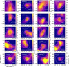 |
Fig. 1 N(H2) maps towards each core in the sample (labelled in the top left corner of every panel). The scale bar shown in the bottom right corner represents a length of 0.05 pc. The white contours show the 20, 40, and 60% levels of the peak value within the central Herschel beam. The solid circles show the APEX pointing and the N(H2) map beam size, whilst the dashed circles show the beam sizes and pointings of APEX for the oH2D+ line. Note the small shift present between the two positions for Oph D, where the oH2D+ beam is not the central LAsMA beam, but one of the external ones (see main text). The shift is, however, smaller than the continuum and APEX resolutions. |
3.2 Continuum data
The methodology we applied (see Sect. 4) requires knowledge of the gas total column density and temperature. We have used available maps of N(H2) and dust temperature Tdust derived from the spectral-energy-distribution (SED) fit of the dust continuum emission detected with Herschel. In particular, for the cores in Ophiuchus, Corona Australis, and Taurus (except for L1544) we used the maps provided by the HGBS survey4. For the remaining cores, we used the maps published in Spezzano et al. (2017, for L1544) and Redaelli et al. (2018, for L429, L694-2, and L183). The HGBS survey provides an H2 column density map at the high angular resolution of 18.2″ (see Palmeirim et al. 2013). In this work, however, we used the products at the larger angular resolution of the SPIRE/500 µm wavelength (≈37″). This is closer to the APEX resolution at ~2 mm, and it is the one available for L183, L429, L694-2, and L1544.
Properties of targeted lines.
4 Analysis and results
To compute ζ2, we applied the analytical formula of Bovino et al. (2020), which was derived from first principles and has the advantage of being model independent. We refer the reader to that paper and to Redaelli et al. (2024) for a complete description of the method’s assumptions and limitations. The approach is based on the detection of the first deuterated form of  , i.e. oH2D+:
 (1)
(1)
where the deuterium fraction of HCO+ is RD = N(DCO+)/N(HCO+), the CO abundance (with respect to H2) is X(CO) = N(CO)/N(H2), and N(oH2D+) is the column density of oH2D+.  is the destruction rate of
  by CO, assumed here to be the main destruction path for
  , while L is the path length over which the column densities are estimated. The
  rate is temperature dependent, and we computed it in each core assuming Tgas = Tdust, hence assuming dust and gas coupling (expected to be efficient at n ≳ 104−5 cm−3; Goldsmith 2001). Sokolov et al. (2017) showed that the difference in the two temperatures can be of the order of 2 K, supporting that this is a good approximation. The rate value is taken from the KIDA5 database (Wakelam et al. 2012), and it presents a modest decrease in the 8–20 K temperature range.
We used the optically thinner C18O to infer the CO abundance, assuming X(CO) = 557 × X(C18O) (Wilson 1999), avoiding opacity issues. For the same reason, the HCO+ deuteration level has been computed from DCO+ and the rarer H13CO+ isotopologue, assuming the isotopic ratio of 12C/13C = 68 (Wilson 1999). In fact, the HCO+ (3−2) transition presents, in most sources, double-peak profiles with asymmetries, which is indicative of self-absorption, and it is not suitable to infer the molecular abundance. The HC18O+ (2−1) is only detected in 60% of the sample, and we do not include it in the analysis. However, we used it later to check the carbon isotopic ratio in the sample (see Sect. 4.3).
4.1 Total gas column density and dust temperature
In order to assign a value of total gas column density N(H2) and dust temperature Tdust to each core, we took the maps listed in Sect. 3.2. We cut square regions of 4′ × 4′ around the cores’ central coordinates. The maps are shown in Fig. 1. We measured the average Tdust and N(H2) in one Herschel beam (37″) around the centre. The values are listed in Table 1.
The cores span the temperature range of 9–20 K, with a mean value of 13 K. The warmest sources all belong to the Corona Australis region (CrA 038, 040, 044, 047, and 050), in particular in the area of the Coronet cluster, which is a well-known active star-forming region (see Chini et al. 2003; Sicilia-Aguilar et al. 2013; Sabatini et al. 2024). The column-density values range from a minimum of 1.7 × 1022 cm−2 (Oph D), to a maximum of 1.16 × 1023 cm−2 (L1544), i.e. approximately one order of magnitude of variation.
4.2 Molecular column densities
The estimate of ζ2 depends on the measurements of column densities of four distinct tracers in Eq. (1). We adopted the constant excitation temperature approach (C-TEX, Caselli et al. 2002) to fit the observed spectra and derive the column density (Ncol) for each species. The fitting procedure is implemented using the PYTHON package PYSPECKIT (Ginsburg & Mirocha 2011; Ginsburg et al. 2022), with the spectroscopic constants listed in Table 2. The partition function of DCO+ is taken from Redaelli et al. (2019); that of C18O, HCO+, H13CO+, and HC18O+ from the CDMS database; and that of oH2D+ from our own calculation based on the energy data provided by CDMS6. We highlight that the transitions from D-bearing species (DCO+, oH2D+) present hyperflne splitting due to the nuclear spin of the deuterium atom. However, the hyperfine structure is usually unresolved given the spectral resolution of our observations (see Caselli & Dore 2005). Since we are not interested in high-precision kinematic measurements in this work (where including the hyperfine structure would be relevant), we neglected it.
The code fits the observed spectra using four free parameters: the line centroid velocity, Vlsr, the line velocity dispersion, σV, the molecular column density, Ncol, and the excitation temperature, Tex. When two transitions from the same species are available, the method assumes that Tex is equal for all transitions. This allows the fitting of Tex and Ncol simultaneously. We estimated the column density of H13CO+ with this approach in the whole sample, except for L1544, Tau 410, and TMC1-C, where H13CO+ (3−2) is not detected7. Similarly, the (3−2) and (4−3) transitions of DCO+ are available for 14 out of 20 targets.
In Fig. 2, we compare the Tex values obtained for DCO+ and H13CO+ in all the cores where this has been possible, also with the Tdust values obtained as described in Sect. 4.1. In general, the excitation temperatures are lower than the corresponding Tdust value by 6% for DCO+ and by 34% for H13CO+. This indicates that the lines are generally sub-thermally excited, i.e. the collisional excitations are not efficient enough to counterbalance the radiative de-excitations, or that the Tdust is overestimating the gas temperature because of line-of-sight averaging (see Sokolov et al. 2017). The first effect is expected as these lines have high critical densities, which can be higher than the average densities of the cores. Interestingly, the DCO+ Tex is on average higher than the H13CO+ one; considering all cases where we have estimates for both, Tex(DCO+) = 1.4 × Tex(H13CO+). We struggle to find an explanation for this behaviour. The fact that the former is estimated using higher J transitions than the latter (hence, with higher critical densities) should point in the opposite direction. Furthermore, H13CO+ is not systematically less abundant than DCO+, which could justify a difference in excitation conditions. The average optical depth of these lines is consistently τ < 1, which rules out opacity issues (see Table A.1). Figure A.19 shows the comparison of the centroid velocity and velocity dispersion values in the whole sample. The Vlsr values are remarkably consistent within each other. The σV values present a higher scatter, and in 68% of sources the DCO+ lines are narrower than the H13CO+ ones. A possible explanation is that the H13CO+ lines are tracing slightly lower densities than the DCO+ lines, as i) deuteration is expected to increase towards the centre, and ii) the angular resolution of H13CO+ data is worse than the DCO+ one, which could cause more lower density material to be intercepted by the H13CO+ emission.
For the species with one detected line, Tex and Ncol are degenerate parameters, and the former must be assumed to estimate the latter. We highlight that this choice is arbitrary, as there is no general prescription to estimate Tex. We proceeded as follows. For H13CO+ and DCO+, in the cases where only one line is detected or available, we computed Tex based on the Tdust values, using the corrective factors computed above (0.94 for DCO+ and 0.66 for H13CO+). For oH2D+ we adopted the same Tex as that of DCO+ . These values are in the 6–22 K range, and they compare well with previous studies of the same molecule (Vastel et al. 2006; Caselli et al. 2008; Redaelli et al. 2021a, 2022). For C18O, we assumed Tdust = Tex, because this is an abundant species with low critical density and it is likely to be thermalised.
Figure 3 showcases an example of the best-fit solutions found towards CrA 151. The lines are well reproduced by the spectral modelling. For a few sources in the sample, however, the line profiles deviate from single Gaussian components. This is the case for Oph 4, for example, which is shown in Fig. 4; there, two clear velocity components (one at ~3.4 km s−1 and one at ~3.9 km s−1) are visible. For the cases where two velocity components can be seen in all transitions, we performed the fit routine previously described with two components, deriving two sets of molecular column densities for the same target. We then summed the two contributions to obtain one column-density value for each species in each core. This is necessary, as the Tdust and total column-density values obtained from the continuum maps cannot distinguish among distinct velocity components. This approach is used for Oph 3 and Oph 4. For other cores where the multiple components are not visible in all tracers or they are too overlapped for the fit to converge, we adopted the single-component procedure, in line with our goal to infer an average ζ2 value across each core. Table 3 summarises the Tex and Ncol values obtained as just described. The complete set of figures for all cores is available in Appendix A. Table A.1 lists the derived best-fit values for the remaining free parameters, line velocity dispersion, and centroid velocity.
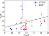 |
Fig. 2 Tex of H13CO+ (blue circles) and DCO+ (red triangles) for all cores where two transitions of the species are available, as a function of Tdust values. The dashed black line shows the 1:1 relation. For cores where two velocity components are identified and fitted, we show the parameters of both. |
4.3 Uncertainties in the column-density estimations
We made several assumptions in the methodology to compute column densities described in Sect. 4.2. Here, we discuss the main ones.
4.3.1 Optical depths
In this work, we used H13CO+ and C18O to trace the total abundance of the corresponding main isotopologues, in the assumption that they are optically thin. To verify this point, the fitting routine implemented in PYSPECKIT returns the peak optical depth, τ, of each transition. We computed the mean and standard deviation of the τ distributions, obtaining: τ(H13CO+ 2 − 1) = 0.44 ± 0.26, τ(H13CO+ 3−2) = 0.26 ± 0.12, and τ(C180 2− 1) = 0.73 ± 0.23. All these values are consistently lower than 1.0, indicating general optically thin conditions.
For completeness, we also report the values for the remaining lines: τ(DCO+ 3 − 2) = 0.58 ± 0.99, τ(DCO+ 4 − 3) = 0.30 ± 0.27, and τ(oH2D+ 11,0 − 11,1) = 0.22 ± 0.20. The mean values are <1.0. All the transitions are on average optically thin across the sample. The optical depth values of the whole sample are available in Table A.1.
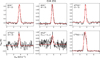 |
Fig. 3 Black histograms show spectra collected towards CrA 151. The transitions are labelled in the top left corner of each panel. The red histograms show the best-fit solution of the spectral fit performed as described in Sect. 4.2. |
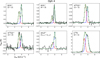 |
Fig. 4 Same as Fig. 3, but for Oph 4. In this core, two velocity components are seen in all the transitions, and we fitted them separately. The red and blue curves show the individual best-fit solutions, whilst the green curve represents the total fit. |
4.3.2 Isotopic ratios
When using rarer isotopologues, we assumed the isotopic ratios 16O/18O = 557 and 12C/13C = 68 to infer the total column densities of the main species. However, recent chemical modelling work showed that carbon fractionation may lead to significant variations (up to a factor of 2) of the 12C/13C ratio (Colzi et al. 2020; Loison et al. 2020). The expected variations of the oxygen isotopic ratio are more modest (Loison et al. 2019). For 12 targets in our sample, we detected the HC18O+ (2 − 1) line. We have, hence, compared the flux ratio of the H13CO+ and HC18O+ transitions (with equal J) to the expected value 557/68 = 8.2. This is appropriate as the two lines have similar spectroscopic constants (see Table 2) and they are optically thin (see previous subsection). We computed integrated intensities over Nch channels with S/N > 3 signal in the 2.8–13.5 km s−1 velocity range. The associated uncertainties are estimated via  . The result is presented in Fig. 5.
The observed H13CO+/HC18O+ values are in the 3.5–32 range, with a weighted average of 8.0, which is very close to the expected value of 557/68 = 8.2. The highest values found in the sample are characterised by the highest uncertainties, as they come from sources where the HC18O+ flux has a low value of S/N = 3–5. For 50% of cases, the measured value is consistent with the expected one, and in 83% of the sample the value is consistent with a variation of a factor of two. Given the uncertainties, we conclude that the isotopic ratios we assumed in the analysis are robust.
Molecular excitation temperatures and column densities obtained by fitting the observed spectral lines.
4.3.3 Beam-filling factor
When computing column densities, we assumed a beam-filling factor of ηff = 1, which means that the molecular emission is more extended than the APEX angular resolution. This needs to be verified, as column densities will be underestimated if ηff < 1 (beam-dilution). At the frequencies of interest, the APEX angular resolution spans the 16–35″ range, which corresponds to 1800–3800 au and 4000–8800 au for the closest and the farthest target, respectively.
Since we do not have maps available to check the real extension of the molecular emission, we instead examined available data from similar sources. For instance, Keown et al. (2016) reported multi-pointing detection of DCO+ (3−2) in L492 and L694-2 (the latter is also present in our sample), and the emission appears well extended beyond 10 000 au. A similar extension is also seen in L1544 (Redaelli et al. 2019). Emission extended over several thousands of au is often reported for H13CO+, even though most studies focus on the (1−0) transition (see e.g. B68, Maret & Bergin 2007; L1498, Maret et al. 2013; several cores in the L1495 filament, Punanova et al. 2018). C18O is an abundant species, which combined with the low critical density of the (2−1) transition makes its emission likely extended (cf. the SEDIGISM survey that used this line to map the ISM in the inner Galaxy by Schuller et al. 2021).
The case of oH2D+ is more complex, as few maps of this species have been observed in the low-mass regime, to our knowledge. Vastel et al. (2006) mapped the oH2D+(11,0 − 11,1) transition in L1544 with the CSO telescope (angular resolution 20″) and detected it over several beams. The map obtained towards Ophiuchus A SM1N with the James Clark Maxwell Telescope (JCMT) shows emission over ~5000 au around the core (Friesen et al. 2014). In Ophiuchus HMM1, Harju et al. (2024) used APEX/LAsMA to map the oH2D+(11,0 − 11,1) line, which is emitted over more than 10 000 au. We conclude that it is reasonable to expect this transition to fill the 16″ APEX beam in the majority of our targets. This is further supported by the fact that for eight cores in the sample, we detected the line not only in the central LAsMA beam, but also in some of the external beams (which are separated by 40″).
Even though we can safely exclude beam-dilution issues, we stress that the difference in beam size at different frequencies might cause the underestimation of the column density of some tracers with respect to that of oH2D+, which presents the highest resolution. In the final results, this problem is mitigated by the fact that the underestimated column densities appear in Eq. (1) as ratios of quantities estimated at similar resolution (RD from the H13CO+ and DCO+ lines at 2 and 1 mm, and X(CO) from CO observations at ~30″ resolution and Herschel maps at 37″). We cannot exclude, however, the underestimation of ζ2 due to that of Ncol(oH2D+).
List of HCO+ deuteration fractions, CO depletion factors, and ζ2 values obtained across the sample.
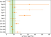 |
Fig. 5 Orange points show measured flux ratio between the H13CO+ and HC18O+ (2−1) lines, in those cores where both transitions are detected (labelled on the y-axis). Error bars show the 3σ level. The vertical dashed orange line shows the weighted average of the sample. The expected value of 557/68 = 8.2 is shown with the vertical green line, and the shaded green area shows a variation of a factor of 2 around it. |
4.4 Deuteration levels and CO depletion factor
We used the column-density values obtained in Sect. 4.2 to compute the deuteration level and the CO abundance in each target. From the latter, we computed the CO depletion factor fD = Xst(CO)/X(CO), where Xst(CO) = 1.2 × 10⁻⁴ is the standard abundance of undepleted CO (Lee et al. 1996; Pineda et al. 2010; Luo et al. 2023). The values are summarised in Table 4, and their correlation is shown in Fig. 6.
The HCO+ deuteration factors are in the range of 0.5–15%, with an average value of 3.4%. Our measured values are in line with other studies of prestellar and starless cores (for example Butner et al. 1995; Tiné et al. 2000). For a direct comparison of individual targets, our derived value (2.8%) in L1544 is consistent with previous results by Redaelli et al. (2019) (3.5%); in L183, our value of 5.2 ± 0.8% is in agreement with the 3–5% range reported by Juvela et al. (2002). The CO depletion factors in our sample are in the 1.3–21 range, which is typical for cold and dense cores, as found by Bacmann et al. (2002), Crapsi et al. (2005), and Lippok et al. (2013).
Both these quantities are strongly correlated with the core dust temperature, as can be seen in Fig. 6, where the colour scale of the data points is determined by the dust-temperature value derived with Herschel. The lowest deuteration and depletion values are found in cores where Tdust > 15 K, becoming comparable to the CO desorption temperature (≈20 K; see Öberg et al. 2011). This immediately lowers the CO depletion factor and, in this physical condition, the efficiency of deuteration processes is also lowered (Dalgarno & Lepp 1984; Ceccarelli et al. 2014a). The highest deuteration level is found in Oph 5, which presents an intermediate temperature within the sample (Tdust = 13.9 K). However, we highlight that the molecular line emission towards this source presents hints of double-velocity components that cannot be fit for all species (cf. the figure in Appendix A). We highlight that in the sources with the lowest fD values, Eq. (1) might underestimate the ζ2 value. This, however, does not change the results of our analysis (see Sect. 5).
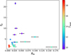 |
Fig. 6 CO depletion factor ƒD as function of HCO+ deuteration fraction. RD in the whole sample. The colour scale is determined by the dust temperature value as reported in Table 1. |
4.5 Estimates of ζ2
Using the RD and X(CO) values, we applied Eq. (1) to infer the cosmic-ray ionisation-rate values. We initially assumed a value of L = 0.1 pc for the source size, which is often regarded as a typical size of low-mass cores in the local ISM (for example Andre et al. 2000; Pineda et al. 2023). A further discussion on the choice of this parameter is presented later. The obtained values and associated uncertainties are reported in the fourth column of Table 4 and in Fig. 7, as a function of the total gas column density N(H2) (upper panel). In the three sources (CrA 044, 047, and 050) where oH2D+ is not detected, we report 3σ upper limits of ζ2. The ζ2 values are scattered over almost two orders of magnitude, ranging from a minimum of 1.3 × 10⁻¹⁸ s−1 to a maximum of 8.5 × 10⁻¹⁷ s−1 (excluding the upper limits). The scatter is significantly larger than the intrinsic uncertainty of the method (estimated as a factor of 2–3, see Redaelli et al. 2024). We discuss possible explanations for the observed scatter in Sect. 5.
The choice of the L value is crucial, as the analytic expression for ζ2 is inversely proportional to it. The topic has been discussed at length in Bovino et al. (2020) and Redaelli et al. (2024). A possible approach is to estimate L from the maps of total column density presented in Sect. 4.1, using the equivalent radius computed from a given contour of N(H2). Choosing which contour is, however, not straightforward. The cores present different contrast levels; i.e. the ratio between the peak N(H2) value at the core’s centre and the surrounding average N(H2) varies significantly, from a factor of a few to more than one order of magnitude. Furthermore, several cores are embedded in crowded environments (in particular in Ophiuchus and Corona). The selection of closed N(H2) contours is, hence, highly dependent on the cores’ parental environments. To take into account the uncertainty associated with the L value, we computed the equivalent diameter corresponding to 40% and 60% of the N(H2) peak at the core’s position. These levels lead to close contours in the whole sample. These values are presented in Table 1. We then computed a range of corresponding ζ2, using the range of L values in Eq. (1), and we report them in the last column of Table 4 and in the upper panel of Fig. 7 using shaded points. For most sources, the ζ2 value obtained using L = 0.1 pc is consistent, within uncertainties, with the range of values computed adopting a variable L, with only three exceptions (CrA 151, L183, and Oph 6)8.
A second possibility for inferring L is to use the detected lines to trace the total gas-volume density and, thus, L = N(H2)/n(H2). In Appendix B, we describe an LVG modelling of the H13CO+ transitions, which are available in the majority of the sample. The results show that even if it is true that in several targets the n(H2) values derived from L = 0.1 pc are underestimated, this underestimation is in line with the method’s error, and this does not affect the main conclusions of this work. We conclude that the choice of L does not significantly impact our analysis and results.
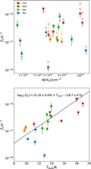 |
Fig. 7 Upper panel: obtained ζ2 values are plotted as function of total gas column density towards each core (including the column density integrated along the line of sight). The solid points and error bars are computed using L = 0.1 pc. The upper limits are shown with downward arrows. The transparent points show the range of ζ2 values obtained when L is computed using the 40% or 60% contours of N(H2). as described in the main text. Lower panel: ζ2 values (computed for L = 0.1 pc) are plotted as a function of the core’s dust temperature, as derived from the Herschel maps. The dashed line shows the linear regression computed in the log10(ζ2)-Tdust plane, and the computed regression coefficients are shown at the top of the panel. In both panels, the data points are colour-coded by parental cloud (red: Corona Australis; green: Ophiuchus; blue: Taurus; orange: isolated sources). |
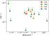 |
Fig. 8 Estimation of ionisation fraction x(e−) using Eq. (2), as a function of the cores’ central total column densities, in the targets with detected oH2D+ emission. We neglected the contribution of N2H+ and N2D+. As in Fig. 7, the data points are colour-coded according to the parental cloud. |
4.6 Ionisation degree and dynamical state of the cores
The ionisation degree of the gas is measured by the electron abundance or electron fraction x(e−). In the assumption that free electrons are donated by neutral species, and that the charge of dust grains is negligible, one can compute x(e−) by assuming the gas charge balance. Latrille et al. (2025) introduced the following proxy for x(e−):
 (2)
(2)
where  . The authors tested it on a set of magneto-hydrodynamic simulations, finding that it reproduces the true x(e−) values with a scatter of 0.5 dex. According to the chemical model of those authors, the main contributions to Eq. (2) come from
  and HCO+. We used this equation to measure x(e−) in each core of the sample, neglecting the diazenylium terms for which we have no estimate, considering only sources with the detection of oH2D+. The obtained values are lower limits to the true gas ionisation degree. Figure 8 shows the resulting plot of x(e−) as a function of the core’s column density.
The obtained values are found in the 10−9−10−8 range, with the majority of cores showing an ionisation degree of 2−4 × 10⁻⁹. These values are in line with literature results in similar sources (Caselli et al. 2002; Maret & Bergin 2007), but they are substantially lower than those derived in NGC1333 by Pineda et al. (2024).
The ionisation degree is directly proportional to the timescale for ambipolar diffusion, tAD; i.e. the process of drift between the neutral species and the ionised one due to imperfect coupling between the two gas flows. In particular, tAD can be computed as (Spitzer 1978; Shu et al. 1987)
 (3)
(3)
We used the computed values of x(e−) to estimate tAD in each core. These values are also lower limits. We compare them to the free-fall timescales (tff), to assess the dynamical stability of the cores:
 (4)
(4)
We adopted µ = 2.33 for the mean molecular weight of the gas and n(H2) = N(H2)/0.1 pc, using the N(H2) tabulated values reported in Table 1. We stress that this approach is underestimating the true central densities of the cores, because it involves a column density value that is averaged on the Herschel beam size and it assumes that the volume density is constant along the line of sight. However, in Appendix B we show that the underestimation is likely of a factor of ~2, and it does not affect the whole sample.
Figure 9 compares the ambipolar diffusion and free-fall timescales in all the sources. Considering the limitations of the method, we can conclude that the derived tAD values are, on average, consistent with, or larger than, the corresponding tff. For the Oph 1–6 cores, this is in line with Bovino et al. (2021), who found that these sources are consistent with model of fast collapse on shorter timescales than the ambipolar diffusion ones.
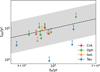 |
Fig. 9 Scatter plot of ambipolar diffusion timescale, tAD, as function of free-fall time, tff, in the targets with detected oH2D+ emission. The tAD values are lower limits, as x(e−) estimated from (2) represents a lower limit. The data points are colour-coded by environment, as in Fig. 7. The dashed line is the 1:1 relation, whilst the shaded area is a 0.5 dex scatter around it (corresponding to the deviation of Eq. (2) from the true value estimated by Latrille et al. 2025). |
5 Discussion
5.1 The role of the environment
The resulting ζ2 values shown in Fig. 7 are coloured by parental cloud. A trend can be seen: cores in Ophiuchus and Corona Australis present, on average, higher ionisation rates than in Taurus or in the more isolated cores (L183, L694-2, and L429, which is found close to the Aquila Rift). The weighted averages in each environment (excluding upper limits) are 〈ζ2〉 = (2.8 ± 0.2) × 10−17s−1 in Corona, (1.76 ± 0.14) × 10−17 s−1 in Ophiuchus, (0.23 ± 0.03) × 10−17 s−1 in Taurus, and (1.22 ± 0.12) × 10−17 s−1 for the three more isolated sources. The differences, in particular between Taurus and Ophiuchus or Corona, are significant considering both the uncertainties reported in Table 4 and the intrinsic error of the method. This points towards the role of the environmental properties in setting the average ionisation rate at the core scales. A similar conclusion was also reached by Sabatini et al. (2023) in high-mass star-forming regions, where the authors highlighted that cores embedded in the same parental clump showed similar ζ2 values, whilst significant differences were found when comparing distinct clumps.
We investigated which environmental physical parameters have the strongest influence on the overall ionisation rate of the cores. From the upper panel of Fig. 7, it appears that the differences in column density among these cores may not be the primary factor contributing to the variations in ζ2. There is no clear correlation between ζ2 and N(H2), and the cores embedded in different clouds cover similar ranges of N(H2) values. On the other hand, the regions analysed differ by dust temperature. Looking at the values in Table 1, the cores’ temperatures are 11–19 K in Corona, ~13.5 K in Ophiuchus, 10–13 K in Taurus, and <10 K in the three isolated sources. The trend is shown in the lower panel of Fig. 7, where we also show the linear regression fit to the values (upper limits excluded) in the semi-logarithmic plane. The Spearman correlation coefficient is 0.65, indicating a high probability of positive correlation between the two quantities. The associated p-value is 0.004 ≪ 0.05; hence, we rejected the null-hypothesis that the two quantities are not correlated. In Appendix B, we show that the correlation remains valid when the gas volume density and the L parameter are inferred from the molecular data instead of the Herschel data.
The different temperatures can be linked to the star-formation activity in the regions. Five of the six cores selected in Corona are found in proximity of the so-called Coronet cluster, which hosts several YSOs at distinct evolutionary stages (see for instance Chini et al. 2003; Sicilia-Aguilar et al. 2013). For CrA 044, 047, and 050 (the latter a known protostellar core), we only report upper limits on oH2D+ and ζ2. This is because the higher temperatures caused by the nearby protostellar activity favour the CO desorption from the dust grains back to the gas phase, as shown by the low values of CO depletion we measured (fD = 1–2). CO, in turn, quickly destroys H2D+. The lowest ζ2 value in the Corona cores is found in CrA 151, which is located ~5 pc away from the Coronet cluster region and is a quiescent core with high levels of deuteration (Redaelli et al. 2025). Ophiuchus is also a very active star-forming region, with ~300 YSO sources identified (Dunham et al. 2015). On the contrary, the cores in Taurus and the isolated sources are found in relatively quieter environments, as proven by both the low temperature values and the low line-velocity dispersions found in these cores (see Table A.1). The main exception is L429, close to the active region of the Aquila Rift. In further support to the scenario just described, L429 presents the highest ζ2 value in this subset, even though the difference is within the uncertainties.
The correlation between the star-formation activity and the ionisation rate of the gas is supported by recent theoretical works, which showed that low-mass protostars can be a source of local re-acceleration of cosmic rays (Padovani et al. 2015, 2016), either at the protostellar surface or in the shocks along the protostellar jets. This can explain the detection of non-thermal radiation in these jets (see e.g. Ainsworth et al. 2014). Regions with strong protostellar activity, therefore, might be characterised by higher levels of ionisation due to CRs, as first noted by Ceccarelli et al. (2014b) and seen in the maps of Pineda et al. (2024). Based on the YSO count, Heiderman et al. (2010) and Evans et al. (2014) estimated the surface density of star formation Σ(SFR) in several Gould Belt Clouds, and reported values of 2.44 M⊙ yr−1 kpc−2 in Ophiuchus, 3.47 in Corona, and 0.15 in Taurus, respectively, which further supports the scenario of correlation between star-formation activity and average ionisation level.
5.2 Comparison with current models of CR propagation
In this section, we discuss the obtained results in the context of available measurements of the CR ionisation rate in the Milky Way and in comparison with the prediction of theoretical models of CR propagation and attenuation. Figure 10 shows a summary of observational estimates taken from literature, as a function of the sources N(H2), with a particular focus on those obtained using the same method we implemented. The only exception is the values at low densities (N(H2) ≲ 1021 cm−2), which refer to diffuse clouds (Obolentseva et al. 2024). These estimates have been re-evaluated ζ2 using 3D visual-extinction maps to infer the volume densities of the sources. As a result, they are a factor of nine lower than previous estimates on average (Indriolo et al. 2007; Indriolo & McCall 2012). The new values obtained in this work are shown with orange stars.
The plots also show the expected trends for the total ionisation rate computed assuming different models of the energy spectrum of protons from Padovani et al. (2022): low (ℒ), high (ℋ), and upper-limit model, 𝒰, which adopts a steep spectral slope of α = −1.2. The high model was introduced initially with the scope of explaining the high ζ2 values obtained in diffuse clouds from  measurements, and it might not be needed anymore given the results of Obolentseva et al. (2024). As discussed in the previous subsection, we do not see a significant decreasing trend with N(H2), as the correlation with the environmental temperature (measured by means of Tdust) is stronger. We also highlight, however, that we explored a relatively small range of column density (less than one order of magnitude). Most of our values are found across the ℒ model, which is the one in agreement with the Voyager data. Nevertheless, we obtained a significant scatter, towards both low and high values. As noted before, we hypothesise that environmental effects are the main driver for it. This strengthens the idea that a universal ζ2 value cannot be adopted, even for sources with similar properties and evolutionary stages.
6 Summary and conclusions
In this work, we estimated the CR ionisation rate, ζ2, in a sample of dense and cold cores embedded in different star-forming regions in the solar neighbourhood. We employed the analytical method of Bovino et al. (2020), further corroborated and updated by Redaelli et al. (2024), which correlates ζ2 with the column density of oH2D+, the CO abundance, and the deuteration fraction of HCO+. To estimate these quantities, we analysed new, high-sensitivity spectroscopic data observed with the APEX single-dish telescope. Furthermore, we used the column density and dust-temperature maps obtained from the analysis of the Herschel data to characterise the cores’ average N(H2) and Tdust values.
We performed a spectral fit to the observed transitions to infer the molecular column density, assuming C-TEX conditions. The estimated deuteration fractions are in the range 0.5–15% and the CO depletion factors span the range ƒD = 1.3–21, which are in agreement with expectations from chemical considerations. Both these parameters correlate with the cores’ temperatures. As Tdust increases and approaches the CO desorption temperature (~20 K), the CO molecules return to the gas-phase (decreasing ƒD) and quickly destroy oH2D+ and, in general, deuterated species, in turn lowering RD.
We inferred the ζ2 value in 17 cores. For three cores, oH2D+ was undetected at the sensitivity level of our observations, and we estimated upper limits on ζ2. To our knowledge, this represents the largest sample of ζ2 measurements in low-mass dense cores obtained with a consistent methodology after the one presented by Caselli et al. (1998). The ζ2 measurements span a range of almost two orders of magnitude, from 1.3 × 10⁻¹⁸ to 8.5 × 10⁻¹⁷ s−1. We do not find a significant correlation with the sources’ total column density. However, we do find significant differences when comparing cores embedded in distinct environments. We detect a significant positive correlation with the cores’ temperatures. We speculate that warmer environments are associated with stronger star-formation activity and they are more affected by protostellar feedback, which causes the temperature rise. This is consistent with theoretical predictions on how low-mass protostars can be local sources of re-acceleration of cosmic rays. Our work strongly suggests that the gas ionisation state (which is crucial for several physical and chemical processes) is not a common property even in sources of similar kinds and evolutionary stages, and, instead, it varies strongly due to both local and environmental effects. Future efforts dedicated to increasing the sample size to more environments will allow a better understanding of which other environmental properties are important for setting the ionisation rate in dense gas.
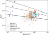 |
Fig. 10 ζ2 as function of N(H2). The theoretical models ℒ (solid black line), ℋ (dashed black line), and 𝒰 (dotted-dashed black line) are taken from Padovani et al. (2022). The new observational estimates obtained in this work are shown with orange stars. The most recent values in the diffuse gas are shown with purple triangles (Obolentseva et al. 2024). We also show literature values in dense gas obtained with the method of Bovino et al. (2020), which are represented with red dots (Sabatini et al. 2020), cyan squares (Sabatini et al. 2023), and shaded grey crosses (Socci et al. 2024). |
Acknowledgements
The authors gracefully acknowledge Dr. Jorma Harju for his help and support. This publication is based on data acquired with the Atacama Pathfinder Experiment (APEX). APEX has been a collaboration between the Max-Planck-Institut fur Radioastronomie, the European Southern Observatory, and the Onsala Space Observatory. This research has made use of data from the Herschel Gould Belt survey (HGBS) project (http://gouldbelt-herschel.cea.fr). The HGBS is a Herschel Key Programme jointly carried out by SPIRE Specialist Astronomy Group 3 (SAG 3), scientists of several institutes in the PACS Consortium (CEA Saclay INAF-IFSI Rome and INAF-Arcetri, KU Leuven, MPIA Heidelberg), and scientists of the Herschel Science Center (HSC). SB acknowledges BASAL Centra de Astrofisica y Tecnologias Afines (CATA), project number AFB-17002. GS acknowledges the project PRIN-MUR 2020 MUR BEYOND-2p (“Astrochemistry beyond the second period elements”, Prot. 2020AFB3FX), the PRIN MUR 2022 FOSSILS (“Chemical origins: linking the fossil composition of the Solar System with the chemistry of protoplanetary disks”, Prot. 2022JC2Y93), the project ASI-Astrobiologia 2023 MIGLIORA (“Modeling Chemical Complexity”, F83C23000800005), the INAF-GO 2023 fundings PROTOSKA (“Exploiting ALMA data to study planet forming disks: preparing the advent of SKA”, C13C23000770005) and the INAF-Minigrant 2023 TRIESTE (“TRacing the chemical hEritage of our originS: from proTo-stars to planEts”; PI: G. Sabatini). GL gratefully acknowledges the financial support of ANID-Subdirección de Capital Humano/Magíster Nacional/2024-22241873 and Millenium Nucleus NCN23_002 (TITANs). MP acknowledges the INAF-Minigrant 2024 ENERGIA (“ExploriNg low-Energy cosmic Rays throuGh theoretical InvestigAtions at INAF”; PI: M. Padovani). The authors thank the anonymous referee for their comments, which helped improved the quality of the manuscript.
Appendix A Spectral fit in the full sample
Figures A.1 to A.18 show the spectral fit performed with PYSPECKIT in each of the cores not shown in the Main Text. Table A.1 summarises the best-fit values obtained for the kinematic parameters (Vlsr and σV), together with the peak optical depth of each transition. Figure A.19 shows the comparison of the centroid velocity and dispersion values for H13CO+ and DCO+.
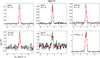 |
Fig. A.1 Similar to Fig. 3, the black histograms show spectra collected towards Oph D. The transitions are labelled in the top left corner of each panel. The red histograms show the spectral fit solutions. |
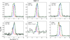 |
Fig. A.4 Same as Fig. A.1, but for Oph 3. As for Oph 4, we performed a two-velocity-component fit. The two distinct components are shown with the red and blue curves, whilst the green curve shows the total fit. |
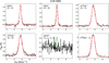 |
Fig. A.9 Same as Fig. A.1, but for CrA 044. In this case, the oH2D+(11,0 − 11,1) line is not detected given the sensitivity. The green curve shows the 3σ upper limit obtained from the column density upper limit listed in Table 3, and the centroid velocity and linewidth of the DCO+ fit. |
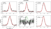 |
Fig. A.10 Same as Fig. A.1, but for CrA 047. In this case, the oH2D+(11,0 − 11,1) line is not detected given the sensitivity. The green curve shows the 3σ upper limit obtained from the column density upper limit listed in Table 3, and the centroid velocity and velocity dispersion of the DCO+ fit. |
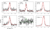 |
Fig. A.11 Same as Fig. A.1, but for CrA 050. In this case, the oH2D+ (11,0 − 11,1) line is not detected given the sensitivity. The green curve shows the 3σ upper limit obtained from the column density upper limit listed in Table 3, and the centroid velocity and velocity dispersion of the DCO+ fit. |
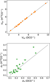 |
Fig. A.19 Comparison of the DCO+ and H13CO+ centroid velocities (top panel) and velocity dispersions (bottom panel). The dashed lines show the 1:1 relation. |
The table summarises the best-fit values for the centroid velocity Vlsr and the velocity dispersion σV obtained with PYSPECKIT, together with the estimated peak opacity of each transition.
Appendix B LVG modelling of the H13CO+ lines
Given the availability of multiple transitions of H13CO+ for almost all the targets, we have used these data to perform simple LVG (large-velocity-gradient) calculation using the RADEX software (van der Tak et al. 2007; Dwiriyanti et al. subm.). This allows us to i) infer n(H2) independently from the Herschel data; ii) re-evaluate the path length L = N(H2)/n(H2); and iii) confirm the sub-thermal excitation for this species. We have used RADEX to compute escape probabilities, adopting the LVG approach. The LAMDA (Leiden Atomic and Molecular DAtabase) file for H13CO+ has been taken from the EMAA database9. We consider para-H2 the main collisional partner. For the sake of simplicity, we have excluded from this analysis the two sources with clear multiple velocity components in all lines (Oph 3 and Oph 4), and the 3 sources with only upper limits for the H13CO+ (3−2) transition (Tau 410, TMC1-C, L1544). The number of analysed targets is 15.
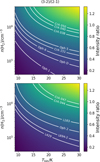 |
Fig. B.1 H13CO+ line intensity ratio (3−2)/(2−1) as a function of H2 volume density versus gas kinetic temperature (Tkin). The plot has been obtained with RADEX, assuming the average H13CO+ column density measured in the sample (9.4 × 1011 cm2). The curves, labelled by object, show the observed values. |
We proceeded to input into the RADEX calculation the H13CO+ column density and the line width (FWHM) derived in Sect. 4.2. We used the dust temperatures in Table 1 as a proxy for the gas temperature, and the gas volume densities obtained from the N(H2) values (Table 1, assuming L = 0.1 pc). We refer to this quantity as n(H2)cont, as it is derived from the Herschel continuum data.
We checked the results, comparing the modelled line intensities with the observed ones. Table B.1 reports the n(H2)cont values for each source, together with the lines peak intensity, both observed and modelled by RADEX. We also list the ratio  . These results show that for 14 out of 15 targets, the (2−1) line intensity is reproduced within a factor of 2, and for the (3−2) lines, this holds for 6 targets. Since the (3−2) line has a better angular resolution and higher critical density, this suggests that the n(H2)cont values underestimate the central volume density. This is expected due to the fact that this quantity is computed from the Herschel low-resolution data, and it represents an average along the line-of-sight and on the beam. Figure B.1 shows the RADEX results concerning the (3−2) to (2−1) line intensity ratio for a grid of gas temperature and n(H2) values. We overplot the curves corresponding to the observed cores. The plot shows that the H13CO+ observations are consistent with volume density values from several ×104cm−3 to 106 cm−3, given the typical cores’ temperatures of 10 – 20 K.
In order to quantify the underestimation, we have increased n(H2) and we ran the LVG computation again. First, we input n(H2) = 2 × n(H2)cont. This is sufficient to reproduce the line instensities within a factor of 2 in all sources except two. The only targets where the emission is still underestimated are L183 (10% for the 2-1, 60% for the 3−2), for which a correction n(H2) = 3 × n(H2)cont is needed, and Tau 420, which is a peculiar source due to the fact that the (3−2) line is brighter than the (2−1) (this is also the only source where we see suprathermal excitation in H13CO+, see Table 3 and Fig. A.19). We can conclude that the n(H2)cont volume densities are underestimated by a factor of ~2.
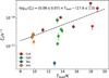 |
Fig. B.2 Plot of ζ2 as a function of Tdust, where the n(H2) values have been re-evaluated from the H13CO+ line emission, as explained in the Text. The sources where we increased n(H2)cont in the LVG calculations are shown with black edges. The dashed black curve shows the linear best fit to the data, in log-linear space. |
We have re-computed the ζ2 values assuming L = 0.05 pc for those 9 sources that needs the correction. The results are shown in Fig B.2, as a function of the dust temperature. We still detect the increase of ζ2 with increasing Tdust. The black curve shows the linear best fit to the data. The trend is shallower and the uncertainties are higher (due to the reduced statistics), but our results still hold. We highlight that the LVG methodology entrails a number of uncertainties, the main ones being i) the Tgas = Tdust assumption; ii) the source geometry, which is ignored.
The RADEX analysis confirms that the H13CO+ transition are subthermally excited. The τ values computed by RADEX are in general in good agreement with those listed in Table A.1, confirming that the lines are optically thin.
Results of the RADEX analysis.
References
- Ainsworth, R. E., Scaife, A. M. M., Ray, T. P., et al. 2014, ApJ, 792, L18 [Google Scholar]
- Andre, P., Ward-Thompson, D., & Barsony, M. 2000, in Protostars and Planets IV, eds. V. Mannings, A. P. Boss, & S. S. Russell, 59 [Google Scholar]
- André, P., Men’shchikov, A., Bontemps, S., et al. 2010, A&A, 518, L102 [NASA ADS] [CrossRef] [EDP Sciences] [Google Scholar]
- Bacmann, A., Lefloch, B., Ceccarelli, C., et al. 2002, A&A, 389, L6 [NASA ADS] [CrossRef] [EDP Sciences] [Google Scholar]
- Belitsky, V., Bylund, M., Desmaris, V., et al. 2018a, A&A, 611, A98 [NASA ADS] [CrossRef] [EDP Sciences] [Google Scholar]
- Belitsky, V., Lapkin, I., Fredrixon, M., et al. 2018b, A&A, 612, A23 [NASA ADS] [CrossRef] [EDP Sciences] [Google Scholar]
- Bovino, S., Ferrada-Chamorro, S., Lupi, A., et al. 2019, ApJ, 887, 224 [NASA ADS] [CrossRef] [Google Scholar]
- Bovino, S., Ferrada-Chamorro, S., Lupi, A., Schleicher, D. R. G., & Caselli, P. 2020, MNRAS, 495, L7 [Google Scholar]
- Bovino, S., Lupi, A., Giannetti, A., et al. 2021, A&A, 654, A34 [NASA ADS] [CrossRef] [EDP Sciences] [Google Scholar]
- Bresnahan, D., Ward-Thompson, D., Kirk, I. M., et al. 2018, A&A, 615, A125 [NASA ADS] [CrossRef] [EDP Sciences] [Google Scholar]
- Butner, H. M., Lada, E. A., & Loren, R. B. 1995, ApJ, 448, 207 [NASA ADS] [CrossRef] [Google Scholar]
- Caselli, P., & Dore, L. 2005, A&A, 433, 1145 [NASA ADS] [CrossRef] [EDP Sciences] [Google Scholar]
- Caselli, P., Walmsley, C. M., Terzieva, R., & Herbst, E. 1998, ApJ, 499, 234 [Google Scholar]
- Caselli, P., Walmsley, C. M., Zucconi, A., et al. 2002, ApJ, 565, 344 [Google Scholar]
- Caselli, P., Vastel, C., Ceccarelli, C., et al. 2008, A&A, 492, 703 [NASA ADS] [CrossRef] [EDP Sciences] [Google Scholar]
- Ceccarelli, C., Caselli, P., Bockelée-Morvan, D., et al. 2014a, in Protostars and Planets VI, eds. H. Beuther, R. S. Klessen, C. P. Dullemond, & T. Henning, 859 [Google Scholar]
- Ceccarelli, C., Dominik, C., López-Sepulcre, A., et al. 2014b, ApJ, 790, L1 [Google Scholar]
- Chini, R., Kämpgen, K., Reipurth, B., et al. 2003, A&A, 409, 235 [NASA ADS] [CrossRef] [EDP Sciences] [Google Scholar]
- Colzi, L., Sipilä, O., Roueff, E., Caselli, P., & Fontani, F. 2020, A&A, 640, A51 [NASA ADS] [CrossRef] [EDP Sciences] [Google Scholar]
- Crapsi, A., Caselli, P., Walmsley, C. M., et al. 2005, ApJ, 619, 379 [Google Scholar]
- Cummings, A. C., Stone, E. C., Heikkila, B. C., et al. 2016, ApJ, 831, 18 [CrossRef] [Google Scholar]
- Dalgarno, A., & Lepp, S. 1984, ApJ, 287, L47 [NASA ADS] [CrossRef] [Google Scholar]
- Dwiriyanti, C., Van der Tak, F. F. S., & de Plaa, I., 2024, A&A, submitted [Google Scholar]
- Dunham, M. M., Allen, L. E., Evans, Neal J., I., et al. 2015, ApIS, 220, 11 [Google Scholar]
- Edenhofer, G., Zucker, C., Frank, P., et al. 2024, A&A, 685, A82 [NASA ADS] [CrossRef] [EDP Sciences] [Google Scholar]
- Evans, Neal J., I., Heiderman, A., & Vutisalchavakul, N. 2014, ApJ, 782, 114 [CrossRef] [Google Scholar]
- Friesen, R. K., Di Francesco, J., Bourke, T. L., et al. 2014, ApJ, 797, 27 [NASA ADS] [CrossRef] [Google Scholar]
- Froebrich, D., & Rowles, J. 2010, MNRAS, 406, 1350 [NASA ADS] [Google Scholar]
- Fuente, A., Cernicharo, J., Roueff, E., et al. 2016, A&A, 593, A94 [NASA ADS] [CrossRef] [EDP Sciences] [Google Scholar]
- Galli, P. A. B., Loinard, L., Bouy, H., et al. 2019, A&A, 630, A137 [NASA ADS] [CrossRef] [EDP Sciences] [Google Scholar]
- Galli, P. A. B., Bouy, H., Olivares, J., et al. 2020, A&A, 634, A98 [NASA ADS] [CrossRef] [EDP Sciences] [Google Scholar]
- Ginsburg, A., & Mirocha, I. 2011, PySpecKit: Python Spectroscopic Toolkit, Astrophysics Source Code Library [record ascl: 1109.001] [Google Scholar]
- Ginsburg, A., Sokolov, V., de Val-Borro, M., et al. 2022, AJ, 163, 291 [NASA ADS] [CrossRef] [Google Scholar]
- Goldsmith, P. F. 2001, ApJ, 557, 736 [Google Scholar]
- Guelin, M., Langer, W. D., Snell, R. L., & Wootten, H. A. 1977, ApJ, 217, L165 [NASA ADS] [CrossRef] [Google Scholar]
- Guelin, M., Langer, W. D., & Wilson, R. W. 1982, A&A, 107, 107 [NASA ADS] [Google Scholar]
- Güsten, R., Nyman, L. Å., Schilke, P., et al. 2006, A&A, 454, L13 [NASA ADS] [CrossRef] [EDP Sciences] [Google Scholar]
- Güsten, R., Baryshev, A., Bell, A., et al. 2008, in Millimeter and Submillimeter Detectors and Instrumentation for Astronomy IV, 7020, eds. W. D. Duncan, W. S. Holland, S. Withington, & J. Zmuidzinas, International Society for Optics and Photonics (SPIE), 702010 [Google Scholar]
- Harju, J., Vastel, C., Sipilä, O., et al. 2024, A&A, 688, A117 [NASA ADS] [CrossRef] [EDP Sciences] [Google Scholar]
- Heiderman, A., Evans, Neal J., I., Allen, L. E., Huard, T., & Heyer, M. 2010, ApJ, 723, 1019 [NASA ADS] [CrossRef] [Google Scholar]
- Hezareh, T., Houde, M., McCoey, C., Vastel, C., & Peng, R. 2008, ApJ, 684, 1221 [NASA ADS] [CrossRef] [Google Scholar]
- Indriolo, N., & McCall, B. J. 2012, ApJ, 745, 91 [NASA ADS] [CrossRef] [Google Scholar]
- Indriolo, N., Geballe, T. R., Oka, T., & McCall, B. J. 2007, ApJ, 671, 1736 [NASA ADS] [CrossRef] [Google Scholar]
- Juvela, M., Mattila, K., Lehtinen, K., et al. 2002, A&A, 382, 583 [NASA ADS] [CrossRef] [EDP Sciences] [Google Scholar]
- Keown, J., Schnee, S., Bourke, T. L., et al. 2016, ApJ, 833, 97 [Google Scholar]
- Kirk, J. M., Ward-Thompson, D., Palmeirim, P., et al. 2013, MNRAS, 432, 1424 [Google Scholar]
- Kong, S., Caselli, P., Tan, J. C., Wakelam, V., & Sipilä, O. 2015, ApJ, 804, 98 [NASA ADS] [CrossRef] [Google Scholar]
- Ladjelate, B., André, P., Könyves, V., et al. 2020, A&A, 638, A74 [NASA ADS] [CrossRef] [EDP Sciences] [Google Scholar]
- Latrille, G., Lupi, A., Bovino, S., et al. 2025, A&A, 699, A126 [NASA ADS] [CrossRef] [EDP Sciences] [Google Scholar]
- Lee, H. H., Bettens, R. P. A., & Herbst, E. 1996, A&AS, 119, 111 [NASA ADS] [CrossRef] [EDP Sciences] [Google Scholar]
- Lippok, N., Launhardt, R., Semenov, D., et al. 2013, A&A, 560, A41 [NASA ADS] [CrossRef] [EDP Sciences] [Google Scholar]
- Loison, J.-C., Wakelam, V., Gratier, P., et al. 2019, MNRAS, 485, 5777 [Google Scholar]
- Loison, J.-C., Wakelam, V., Gratier, P., & Hickson, K. M. 2020, MNRAS, 498, 4663 [Google Scholar]
- Luo, G., Zhang, Z.-Y., Bisbas, T. G., et al. 2023, ApJ, 946, 91 [NASA ADS] [CrossRef] [Google Scholar]
- Maret, S., & Bergin, E. A. 2007, ApJ, 664, 956 [Google Scholar]
- Maret, S., Bergin, E. A., & Tafalla, M. 2013, A&A, 559, A53 [NASA ADS] [CrossRef] [EDP Sciences] [Google Scholar]
- Marsh, K. A., Kirk, J. M., André, P., et al. 2016, MNRAS, 459, 342 [Google Scholar]
- McCall, B. J., Huneycutt, A. J., Saykally, R. J., et al. 2003, Nature, 422, 500 [CrossRef] [Google Scholar]
- Mouschovias, T. C., & Spitzer, L., J. 1976, ApJ, 210, 326 [NASA ADS] [CrossRef] [Google Scholar]
- Müller, H. S., Schläder, F., Stutzki, J., & Winnewisser, G. 2005, J. Mol. Struct., 742, 215 [CrossRef] [Google Scholar]
- Neufeld, D. A., Welty, D. E., Ivlev, A. V., et al., 2024, ApJ, 973, 143 [Google Scholar]
- Öberg, K. I., Murray-Clay, R., & Bergin, E. A. 2011, ApJ, 743, L16 [Google Scholar]
- Obolentseva, M., Ivlev, A. V., Silsbee, K., et al. 2024, ApJ, 973, 142 [NASA ADS] [CrossRef] [Google Scholar]
- Oka, T. 2019, Philos. Trans. Roy. Soc. London Ser. A, 377, 20180402 [Google Scholar]
- Ortiz-León, G. N., Loinard, L., Dzib, S. A., et al. 2018, ApJ, 869, L33 [Google Scholar]
- Padovani, M., Galli, D., & Glassgold, A. E. 2009, A&A, 501, 619 [NASA ADS] [CrossRef] [EDP Sciences] [Google Scholar]
- Padovani, M., Hennebelle, P., Marcowith, A., & Ferrière, K. 2015, A&A, 582, L13 [NASA ADS] [CrossRef] [EDP Sciences] [Google Scholar]
- Padovani, M., Marcowith, A., Hennebelle, P., & Ferrière, K. 2016, A&A, 590, A8 [NASA ADS] [CrossRef] [EDP Sciences] [Google Scholar]
- Padovani, M., Ivlev, A. V., Galli, D., & Caselli, P. 2018, A&A, 614, A111 [NASA ADS] [CrossRef] [EDP Sciences] [Google Scholar]
- Padovani, M., Ivlev, A. V., Galli, D., et al. 2020, Space Sci. Rev., 216, 29 [CrossRef] [Google Scholar]
- Padovani, M., Bialy, S., Galli, D., et al. 2022, A&A, 658, A189 [NASA ADS] [CrossRef] [EDP Sciences] [Google Scholar]
- Palmeirim, P., André, P., Kirk, J., et al. 2013, A&A, 550, A38 [NASA ADS] [CrossRef] [EDP Sciences] [Google Scholar]
- Pety, J. 2005, in SF2A-2005: Semaine de l’Astrophysique Francaise, eds. F. Casoli, T. Contini, J. M. Hameury, & L. Pagani, 721 [Google Scholar]
- Pineda, J. L., Goldsmith, P. F., Chapman, N., et al. 2010, ApJ, 721, 686 [NASA ADS] [CrossRef] [Google Scholar]
- Pineda, J. E., Arzoumanian, D., Andre, P., et al. 2023, in Astronomical Society of the Pacific Conference Series, 534, Protostars and Planets VII, eds. S. Inutsuka, Y. Aikawa, T. Muto, K. Tomida, & M. Tamura, 233 [NASA ADS] [Google Scholar]
- Pineda, J. E., Sipilä, O., Segura-Cox, D. M., et al. 2024, A&A, 686, A162 [NASA ADS] [CrossRef] [EDP Sciences] [Google Scholar]
- Punanova, A., Caselli, P., Pineda, J. E., et al. 2018, A&A, 617, A27 [NASA ADS] [CrossRef] [EDP Sciences] [Google Scholar]
- Redaelli, E., Bizzocchi, L., Caselli, P., et al. 2018, A&A, 617, A7 [NASA ADS] [CrossRef] [EDP Sciences] [Google Scholar]
- Redaelli, E., Bizzocchi, L., Caselli, P., et al. 2019, A&A, 629, A15 [NASA ADS] [CrossRef] [EDP Sciences] [Google Scholar]
- Redaelli, E., Bovino, S., Giannetti, A., et al. 2021a, A&A, 650, A202 [NASA ADS] [CrossRef] [EDP Sciences] [Google Scholar]
- Redaelli, E., Sipilä, O., Padovani, M., et al. 2021b, A&A, 656, A109 [NASA ADS] [CrossRef] [EDP Sciences] [Google Scholar]
- Redaelli, E., Bovino, S., Sanhueza, P., et al. 2022, ApJ, 936, 169 [NASA ADS] [CrossRef] [Google Scholar]
- Redaelli, E., Bovino, S., Lupi, A., et al. 2024, A&A, 685, A67 [NASA ADS] [CrossRef] [EDP Sciences] [Google Scholar]
- Redaelli, E., Spezzano, S., Caselli, P., et al. 2025, A&A, 696, A171 [NASA ADS] [CrossRef] [EDP Sciences] [Google Scholar]
- Roy, A., André, P., Palmeirim, P., et al. 2014, A&A, 562, A138 [NASA ADS] [CrossRef] [EDP Sciences] [Google Scholar]
- Sabatini, G., Bovino, S., Giannetti, A., et al. 2020, A&A, 644, A34 [EDP Sciences] [Google Scholar]
- Sabatini, G., Bovino, S., & Redaelli, E. 2023, ApJ, 947, L18 [NASA ADS] [CrossRef] [Google Scholar]
- Sabatini, G., Podio, L., Codella, C., et al. 2024, A&A, 684, L12 [NASA ADS] [CrossRef] [EDP Sciences] [Google Scholar]
- Schuller, F., Urquhart, J. S., Csengeri, T., et al. 2021, MNRAS, 500, 3064 [Google Scholar]
- Shu, F. H., Adams, F. C., & Lizano, S. 1987, ARA&A, 25, 23 [Google Scholar]
- Sicilia-Aguilar, A., Henning, T., Linz, H., et al. 2013, A&A, 551, A34 [NASA ADS] [CrossRef] [EDP Sciences] [Google Scholar]
- Sipilä, O., Caselli, P., & Harju, J. 2015, A&A, 578, A55 [Google Scholar]
- Socci, A., Sabatini, G., Padovani, M., Bovino, S., & Hacar, A. 2024, A&A, 687, A70 [NASA ADS] [CrossRef] [EDP Sciences] [Google Scholar]
- Sokolov, V., Wang, K., Pineda, J. E., et al. 2017, A&A, 606, A133 [NASA ADS] [CrossRef] [EDP Sciences] [Google Scholar]
- Spezzano, S., Caselli, P., Bizzocchi, L., Giuliano, B. M., & Lattanzi, V. 2017, A&A, 606, A82 [NASA ADS] [CrossRef] [EDP Sciences] [Google Scholar]
- Spezzano, S., Redaelli, E., Caselli, P., et al. 2025, A&A, 694, A27 [NASA ADS] [CrossRef] [EDP Sciences] [Google Scholar]
- Spitzer, L. 1978, Physical Processes in the Interstellar Medium [Google Scholar]
- Stone, E. C., Cummings, A. C., Heikkila, B. C., & Lal, N. 2019, Nat. Astron., 3, 1013 [NASA ADS] [CrossRef] [Google Scholar]
- Tiné, S., Roueff, E., Falgarone, E., Gerin, M., & Pineau des Forêts, G. 2000, A&A, 356, 1039 [NASA ADS] [Google Scholar]
- van der Tak, F. F. S., Black, J. H., Schöier, F. L., Jansen, D. J., & van Dishoeck, E. F. 2007, A&A, 468, 627 [NASA ADS] [CrossRef] [EDP Sciences] [Google Scholar]
- van Dishoeck, E. F., & Black, J. H. 1982, ApJ, 258, 533 [NASA ADS] [CrossRef] [Google Scholar]
- Vastel, C., Caselli, P., Ceccarelli, C., et al. 2006, ApJ, 645, 1198 [NASA ADS] [CrossRef] [Google Scholar]
- Wakelam, V., Herbst, E., Loison, J. C., et al. 2012, ApJS, 199, 21 [Google Scholar]
- Wilson, T. L. 1999, Rep. Progr. Phys., 62, 143 [CrossRef] [Google Scholar]
- Wootten, A., Snell, R., & Glassgold, A. E. 1979, ApJ, 234, 876 [NASA ADS] [CrossRef] [Google Scholar]
All data available at http://gouldbelt-herschel.cea.fr/archives
Available at http://www.iram.fr/IRAMFR/GILDAS/
The detailed references are Bresnahan et al. (2018) for Corona; Roy et al. (2014) and Ladjelate et al. (2020) for Ophiuchus; and Palmeirim et al. (2013) for Taurus.
The partition function of oH2D+ at the temperature T is computed using  , where ɡu,i and Eu,i are the degeneracy and energy of the upper i level.
In L1544, a tentative detection of H13CO+ (3−2) was found, but the low S/N (~3) prevents the fit from converging.
Here, we do not take into considerations the three sources with upper limits on oH2D+.
All Tables
Molecular excitation temperatures and column densities obtained by fitting the observed spectral lines.
List of HCO+ deuteration fractions, CO depletion factors, and ζ2 values obtained across the sample.
The table summarises the best-fit values for the centroid velocity Vlsr and the velocity dispersion σV obtained with PYSPECKIT, together with the estimated peak opacity of each transition.
All Figures
|
Fig. 1 N(H2) maps towards each core in the sample (labelled in the top left corner of every panel). The scale bar shown in the bottom right corner represents a length of 0.05 pc. The white contours show the 20, 40, and 60% levels of the peak value within the central Herschel beam. The solid circles show the APEX pointing and the N(H2) map beam size, whilst the dashed circles show the beam sizes and pointings of APEX for the oH2D+ line. Note the small shift present between the two positions for Oph D, where the oH2D+ beam is not the central LAsMA beam, but one of the external ones (see main text). The shift is, however, smaller than the continuum and APEX resolutions. |
| In the text | |
|
Fig. 2 Tex of H13CO+ (blue circles) and DCO+ (red triangles) for all cores where two transitions of the species are available, as a function of Tdust values. The dashed black line shows the 1:1 relation. For cores where two velocity components are identified and fitted, we show the parameters of both. |
| In the text | |
|
Fig. 3 Black histograms show spectra collected towards CrA 151. The transitions are labelled in the top left corner of each panel. The red histograms show the best-fit solution of the spectral fit performed as described in Sect. 4.2. |
| In the text | |
|
Fig. 4 Same as Fig. 3, but for Oph 4. In this core, two velocity components are seen in all the transitions, and we fitted them separately. The red and blue curves show the individual best-fit solutions, whilst the green curve represents the total fit. |
| In the text | |
|
Fig. 5 Orange points show measured flux ratio between the H13CO+ and HC18O+ (2−1) lines, in those cores where both transitions are detected (labelled on the y-axis). Error bars show the 3σ level. The vertical dashed orange line shows the weighted average of the sample. The expected value of 557/68 = 8.2 is shown with the vertical green line, and the shaded green area shows a variation of a factor of 2 around it. |
| In the text | |
|
Fig. 6 CO depletion factor ƒD as function of HCO+ deuteration fraction. RD in the whole sample. The colour scale is determined by the dust temperature value as reported in Table 1. |
| In the text | |
|
Fig. 7 Upper panel: obtained ζ2 values are plotted as function of total gas column density towards each core (including the column density integrated along the line of sight). The solid points and error bars are computed using L = 0.1 pc. The upper limits are shown with downward arrows. The transparent points show the range of ζ2 values obtained when L is computed using the 40% or 60% contours of N(H2). as described in the main text. Lower panel: ζ2 values (computed for L = 0.1 pc) are plotted as a function of the core’s dust temperature, as derived from the Herschel maps. The dashed line shows the linear regression computed in the log10(ζ2)-Tdust plane, and the computed regression coefficients are shown at the top of the panel. In both panels, the data points are colour-coded by parental cloud (red: Corona Australis; green: Ophiuchus; blue: Taurus; orange: isolated sources). |
| In the text | |
|
Fig. 8 Estimation of ionisation fraction x(e−) using Eq. (2), as a function of the cores’ central total column densities, in the targets with detected oH2D+ emission. We neglected the contribution of N2H+ and N2D+. As in Fig. 7, the data points are colour-coded according to the parental cloud. |
| In the text | |
|
Fig. 9 Scatter plot of ambipolar diffusion timescale, tAD, as function of free-fall time, tff, in the targets with detected oH2D+ emission. The tAD values are lower limits, as x(e−) estimated from (2) represents a lower limit. The data points are colour-coded by environment, as in Fig. 7. The dashed line is the 1:1 relation, whilst the shaded area is a 0.5 dex scatter around it (corresponding to the deviation of Eq. (2) from the true value estimated by Latrille et al. 2025). |
| In the text | |
|
Fig. 10 ζ2 as function of N(H2). The theoretical models ℒ (solid black line), ℋ (dashed black line), and 𝒰 (dotted-dashed black line) are taken from Padovani et al. (2022). The new observational estimates obtained in this work are shown with orange stars. The most recent values in the diffuse gas are shown with purple triangles (Obolentseva et al. 2024). We also show literature values in dense gas obtained with the method of Bovino et al. (2020), which are represented with red dots (Sabatini et al. 2020), cyan squares (Sabatini et al. 2023), and shaded grey crosses (Socci et al. 2024). |
| In the text | |
|
Fig. A.1 Similar to Fig. 3, the black histograms show spectra collected towards Oph D. The transitions are labelled in the top left corner of each panel. The red histograms show the spectral fit solutions. |
| In the text | |
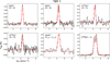 |
Fig. A.2 Same as Fig. A.1, but for Oph 1. |
| In the text | |
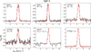 |
Fig. A.3 Same as Fig. A.1, but for Oph 2. |
| In the text | |
|
Fig. A.4 Same as Fig. A.1, but for Oph 3. As for Oph 4, we performed a two-velocity-component fit. The two distinct components are shown with the red and blue curves, whilst the green curve shows the total fit. |
| In the text | |
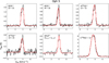 |
Fig. A.5 Same as Fig. A.1, but for Oph 5. |
| In the text | |
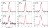 |
Fig. A.6 Same as Fig. A.1, but for Oph 6. |
| In the text | |
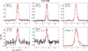 |
Fig. A.7 Same as Fig. A.1, but for CrA 038. |
| In the text | |
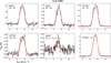 |
Fig. A.8 Same as Fig. A.1, but for CrA 040. |
| In the text | |
|
Fig. A.9 Same as Fig. A.1, but for CrA 044. In this case, the oH2D+(11,0 − 11,1) line is not detected given the sensitivity. The green curve shows the 3σ upper limit obtained from the column density upper limit listed in Table 3, and the centroid velocity and linewidth of the DCO+ fit. |
| In the text | |
|
Fig. A.10 Same as Fig. A.1, but for CrA 047. In this case, the oH2D+(11,0 − 11,1) line is not detected given the sensitivity. The green curve shows the 3σ upper limit obtained from the column density upper limit listed in Table 3, and the centroid velocity and velocity dispersion of the DCO+ fit. |
| In the text | |
|
Fig. A.11 Same as Fig. A.1, but for CrA 050. In this case, the oH2D+ (11,0 − 11,1) line is not detected given the sensitivity. The green curve shows the 3σ upper limit obtained from the column density upper limit listed in Table 3, and the centroid velocity and velocity dispersion of the DCO+ fit. |
| In the text | |
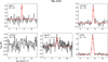 |
Fig. A.12 Same as Fig. A.1, but for Tau 410. |
| In the text | |
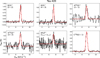 |
Fig. A.13 Same as Fig. A.1, but for Tau 420. |
| In the text | |
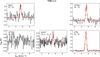 |
Fig. A.14 Same as Fig. A.1, but for TMC1-C. |
| In the text | |
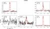 |
Fig. A.15 Same as Fig. A.1, but for L1544. |
| In the text | |
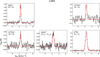 |
Fig. A.16 Same as Fig. A.1, but for L183. |
| In the text | |
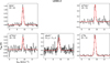 |
Fig. A.17 Same as Fig. A.1, but for L694-2. |
| In the text | |
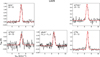 |
Fig. A.18 Same as Fig. A.1, but for L429. |
| In the text | |
|
Fig. A.19 Comparison of the DCO+ and H13CO+ centroid velocities (top panel) and velocity dispersions (bottom panel). The dashed lines show the 1:1 relation. |
| In the text | |
|
Fig. B.1 H13CO+ line intensity ratio (3−2)/(2−1) as a function of H2 volume density versus gas kinetic temperature (Tkin). The plot has been obtained with RADEX, assuming the average H13CO+ column density measured in the sample (9.4 × 1011 cm2). The curves, labelled by object, show the observed values. |
| In the text | |
|
Fig. B.2 Plot of ζ2 as a function of Tdust, where the n(H2) values have been re-evaluated from the H13CO+ line emission, as explained in the Text. The sources where we increased n(H2)cont in the LVG calculations are shown with black edges. The dashed black curve shows the linear best fit to the data, in log-linear space. |
| In the text | |
Current usage metrics show cumulative count of Article Views (full-text article views including HTML views, PDF and ePub downloads, according to the available data) and Abstracts Views on Vision4Press platform.
Data correspond to usage on the plateform after 2015. The current usage metrics is available 48-96 hours after online publication and is updated daily on week days.
Initial download of the metrics may take a while.