| Issue |
A&A
Volume 702, October 2025
|
|
|---|---|---|
| Article Number | A71 | |
| Number of page(s) | 20 | |
| Section | Numerical methods and codes | |
| DOI | https://doi.org/10.1051/0004-6361/202453266 | |
| Published online | 07 October 2025 | |
Mapping synthetic observations to pre-stellar core models: An interpretable machine learning approach
1
Max-Planck-Institut für Extraterrestrische Physik,
Giessenbachstraße 1,
85748
Garching,
Germany
2
Exzellenzcluster Origins,
Boltzmannstr. 2,
85748
Garching,
Germany
3
INAF Osservatorio Astrofisico di Arcetri,
Largo E. Fermi 5,
50125
Firenze,
Italy
4
European Spallation Source ERIC, Data Management and Software Centre,
Asmussens Allé 305,
2800
Lyngby,
Denmark
5
European Southern Observatory,
Karl-Schwarzschild-Straße 2,
85748
Garching,
Germany
6
Chemistry Department, Sapienza University of Rome,
P.le A. Moro,
00185
Roma,
Italy
7
Departamento de Astronomía, Facultad Ciencias Físicas y Matemáticas, Universidad de Concepción,
Av. Esteban Iturra s/n Barrio Universitario, Casilla 160,
Concepción,
Chile
★ Corresponding author: This email address is being protected from spambots. You need JavaScript enabled to view it.
Received:
2
December
2024
Accepted:
6
February
2025
Abstract
Context. We present a methodology for linking the information in the synthetic spectra with the actual information in the simulated models (i.e., their physical properties), in particular to determine where the information resides in the spectra.
Aims. We employed a 1D gravitational collapse model with advanced thermochemistry, from which we generated synthetic spectra. We then used neural network emulations and the SHapley Additive exPlanations (SHAP), a machine learning technique, to connect the models’ properties to the specific spectral features.
Methods. Thanks to interpretable machine learning, we find several correlations between synthetic lines and some of the key model parameters, such as the cosmic-ray ionization radial profile, the central density, or the abundance of various species, suggesting that most of the information is retained in the observational process.
Results. Our procedure can be generalized to similar scenarios to quantify the amount of information lost in the real observations. We also point out the limitations for future applicability.
Key words: astrochemistry / methods: data analysis / methods: numerical
© The Authors 2025
 Open Access article, published by EDP Sciences, under the terms of the Creative Commons Attribution License (https://creativecommons.org/licenses/by/4.0), which permits unrestricted use, distribution, and reproduction in any medium, provided the original work is properly cited.
This article is published in open access under the Subscribe to Open model.
Open Access funding provided by Max Planck Society.
1 Introduction
Pre-stellar cores are cold and quiescent regions in molecular clouds representing the initial conditions for star formation (Caselli 2011). They reveal complex chemical structures, with different molecular species tracing the different properties of these objects (e.g., Bergin et al. 2005; Spezzano et al. 2017). This chemical variety makes it possible to employ some of the chemical species to infer physical properties, such as the object's geometry (Tritsis et al. 2016), temperature (Crapsi et al. 2007; Harju et al. 2017; Pineda et al. 2022), volume density (Lin et al. 2022), and gas kinematics (Caselli et al. 2002; Punanova et al. 2018; Redaelli et al. 2022).
In addition to these properties, estimating the cosmic-ray ionization rate of H2 (ζ) from observations remains a complex task since each method carries some degree of uncertainty, mainly due to unknown rate coefficients in chemical networks and the source size. In a diffuse interstellar medium (AV ≤ 1 mag), ζ can be inferred from H3+ absorption lines (e.g., Indriolo & McCall 2012) and from estimating the gas volume density nH2 from 3D mapping of the dust extinction using Gaia data coupled with chemical modeling of C2 spectra (Neufeld et al. 2024; Obolentseva et al. 2024), the latter obtaining lower values of ζ. At higher column densities, a larger number of methods have been developed using different molecular tracers (e.g., Caselli et al. 1998; Bovino et al. 2020; Redaelli et al. 2024). For a recent review, we refer to Padovani & Gaches (2024).
However, the exact dynamical model that best describes prestellar core evolution remains uncertain, with various models producing different predictions for gas molecular transitions, not only in pre-stellar cores (e.g., Keto & Caselli 2008; Sipilä et al. 2022), but also in other objects, such as molecular clouds (Priestley et al. 2023). This suggests that determining the link between the features observed in the synthetic observations and the corresponding simulated objects is crucial to understanding the physical structure and dynamic evolution of pre-stellar cores (Jensen et al. 2023).
Inferring the physical properties from the features of observed spectra is a well-established methodology (Kaufman et al. 1999; Pety et al. 2017). However, only recent studies have explored the use of machine learning techniques to predict the gas parameters from observational data. For example, using random forests and multi-molecule line emissions, Gratier et al. (2021) inferred the H2 column density of molecular clouds from radio observations. Behrens et al. (2024) employed standard neural networks to determine the cosmic-ray ionization rate from observed spectra of HCN and HNC. In photon-dominated regions, Einig et al. (2024) found the most effective combination of tracers by comparing the mutual information of a physical parameter and different sets of lines using an approach based on conditional differential entropy. Shimajiri et al. (2023) used the Extra Trees Regressor to predict the H2 column density from CO isotopologs. With an explanatory regression model Diop et al. (2024) studied the dependence of CO spatial density on several protoplanetary disk parameters, including the gas density and the cosmic-ray ionization rate.
Finally, Heyl et al. (2023) and later Asensio Ramos et al. (2024) employed interpretable machine learning to determine how key physical parameters influence the observed molecular abundances. In particular, they assigned to each model’s parameter feature a contribution value to a specific chemical species prediction using SHapley Additive exPlanations (SHAP, Lundberg & Lee 2017), a technique based on cooperative game theory principles to interpret the predictions of a machine learning emulator. We employ a similar approach, but in our case, we invert the emulation process to predict the model parameters from the observed spectra. Thanks to SHAP, we can determine the contribution of each spectral feature to each physical parameter.
In Sect. 2, we first give an overview of the different steps. In Sect. 3 we describe the procedure employed to generate the gravitational collapse models, their thermochemical evolution, and the post-processing with a large chemical network. In Sect. 4, we give the details of the synthetic spectra calculations. In Sect. 5, we report the forward and backward emulation of the procedures described to date, while Sect. 6 is dedicated to the interpretation of the results by using SHAP. Finally, in Sects. 7 and 8 we report the limitations of our approach and present our conclusions with future outlooks.
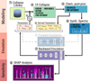 |
Fig. 1 Schematic diagram of the procedure employed in this work. The top part represents the modeling steps: (1) generating the library of gravitational collapse models; (2) randomly selecting the base models depending on the global parameters; (3) evolving the thermochemistry in the collapse model; (4) including additional chemistry with post-processing; (5) obtaining the derived quantities (e.g., the abundances of some key species); and (6) producing the synthetic spectra. The middle part is the emulation: (7a) forward emulation, from parameters to spectra; (7) backward emulation, from spectra to parameters. The sensitivity using SHAP at the bottom (8) is where we perturb the neural network input features to determine the impact on the outputs. |
2 Analysis steps
To connect numerical models of pre-stellar cores and synthetic observations, we employed some of the recent advancements in interpretable machine learning. The general concept is illustrated in Fig. 1. In particular, we generate a library of 1D hydrodynamical isothermal collapse models (label 1 in the figure). This provides the Lagrangian time-dependent tracer particles. We randomized a set of parameters to select and generate 3000 collapse models with different conditions that will evolve in time with a relatively small chemical network to determine the temperature evolution (2-3). Since we only used a simplified chemical network to determine the gas and dust temperature in the previous step, the following post-processing stage gives us a more complicated chemistry than the simple one needed for cooling and heating (4). We do not limit our analysis to the randomized parameters but also to derived quantities, such as the cosmic-ray ionization radial profile or the abundances of the various molecules (5). Thanks to the additional chemical species, we generate a database of synthetic spectra for several molecules and transitions (6). At this stage, we have a correspondence between initial parameters and spectra. This allows us to use a standard neural network to emulate the backward process (from spectra to parameters, 7) and, less relevant to the aims of this paper, the forward process (from parameters to spectra, 7a). In this way, we have a differentiable operator to determine the impact of the input (i.e., each velocity channel in the synthetic observations) onto the output (i.e., each physical parameter in the model). The weapon of choice for this analysis is the SHapley Additive exPlanations or SHAP (8).
3 Model sample generation
31 Collapse model
Before selecting the random parameters, we generate a library of collapse models for different initial masses (M). In this context, we assume that the temperature variations are negligible for the dynamics, but not for the chemistry. For this reason, we can generate the time-dependent trajectories of the gas elements in advance, assuming isothermality, and compute the gas and dust temperature in a second stage (Sect. 3.3).
To model the hydrodynamical collapse, we use the fully-implicit Godunov Lagrangian 1D code SINERGHY1D, which solves standard non-magnetized fluid equations (Vaytet et al. 2012, 2013; Vaytet & Haugbølle 2017). In this case, we assume the collapse to be isothermal, similar to the one described in Larson (1969) and Penston (1969). Setting the mass M of the collapsing region allows the collapsing radius Rc and the corresponding initial density ρ0 to be computed as
 (1)
(1)
where  is the isothermal speed of sound, G the gravitational constant, kB the Boltzmann constant, and mp the proton mass. We assume constant temperature T = 10 K and mean molecular weight μ = 2.34, noticing that modifying these parameters within the ranges allowed by the collapse of a pre-stellar core plays a minor role in the evolution of the system. Considering that the gravitational pull on a volume element located at radius r is proportional to
  (i.e., spherical self-gravity), we obtain a set of collapse profiles at different times. As expected, the collapse is self-similar. We note that the Larson collapse was discarded by Keto et al. (2015) for the special case of L1544. However, the Larson (1969) model is easier to parametrize, and we use it here as an example. Other contraction models will be considered in future work.
To mimic the presence of magnetic pressure or similar physical processes that might reduce the collapse velocity, we introduce a unitless factor τ to slow down the collapse. This is conceptually equivalent to slowing each Lagrangian particle’s “clock” by a factor τ (see, e.g., Kong et al. 2015; Bovino et al. 2021). Therefore, the hydrodynamical timestep of each particle becomes ∆t = τ∆tH and the corresponding radial velocity  , where the subscript H indicates the quantity computed by the hydrodynamical code.
3.2 Parameter generation
To generate one of the 3000 pre-stellar cores in our synthetic population sample, we perform the following steps:
Randomly select an initial mass M in the range 5M⊙ to 15 M⊙ and the corresponding collapse model calculated as described in Sect. 3.1;
Select a maximum central number density using a uniform random generator in the logarithmic space within a range of 105 cm−3 and 107 cm−3. This corresponds to a specific maximum time tmax that depends on the model selected in the first step;
Randomize the visual extinction at the limits of the computational domain1 (Av,0) between 2 and 7 mag. This determines the corresponding column density as Av,0 = 1.0638 × 10⁻²¹ N0, where the multiplying factor is in units of mag cm2. The aim is to simulate the presence of an external cloud environment;
Randomize the time factor τ uniformly between 1 and 10 and scaling timesteps, velocities, and adiabatic heating accordingly;
Randomize the radially uniform and non-time-dependent velocity dispersion of the turbulence between rσ = 0.01 and rσ = 0.33 times the maximum of the absolute value of the velocity during the collapse (i.e., σ3 = rσ max(|υ|));
Compute the time-dependent gas and dust temperature radial profile using a 275-reactions chemical network, as described in Sect. 3.3;
Compute the time-dependent gas chemistry using gas and dust temperature from the previous step, but using a 4406-reactions chemical network, as described in Sect. 3.4;
These steps are repeated for all the 3000 models using the aforementioned randomization. This procedure will generate a radial profile of every quantity (e.g., density, chemical abundances, temperature, cosmic-ray ionization rate) for each model at each time step. Still, we limit our analyses to t = tmax.
An example model from the set of synthetic cores is shown in Fig. 2, where the upper left panel shows the total number density radial profile obtained with the hydrodynamical code at tmax, while the upper right panel reports the radial velocity profile. The temperature and the cooling and heating process in the upper right and lower left panels are discussed in Sect. 3.3, while the chemical abundances in the lower right panel are discussed in Sect. 3.4. The other models show similar radial profiles.
3.3 Thermochemistry
In order to generate various temperature profiles, we use a simplified chemical network. Since each Lagrangian particle has defined time, density, velocity, and position, we can compute its time-dependent thermochemistry. To this end, we use the thermochemistry code KROME (Grassi et al. 2014), with a limited chemical network of 36 species (see Appendix A). We include 275 reactions from the react_COthin_ice network from KROME, mainly based on Glover et al. (2010) chemistry. More in detail, it employs gas chemistry, Av-based photochemistry, cosmic-ray chemistry, and CO and water evaporation and freeze-out. The network includes H2 (Draine & Bertoldi 1996; Richings et al. 2014) and CO (Visser et al. 2009) self-shielding parametrizations. This set of reactions is optimized to produce the correct amount of coolant species and, therefore, the correct gas temperature (see, e.g., Glover & Clark 2012; Gong et al. 2017).
The initial conditions are the same for all the Lagrangian particles that, at time zero, have the same density by construction, as described in Sect. 3.1. For this chemical network, the initial conditions are reported in Table 1, labeled as small and both. The chemical initial conditions play a major role in the timedependent chemical evolution of several species, for example, HCN (Hily-Blant et al. 2010). In this work, we arbitrarily decided to use the initial conditions of Sipilä & Caselli (2018), but other initial conditions could also be employed (e.g., Bovino et al. 2019). Given the aims of the present work, we do not explore this issue further.
We use a radial-dependent cosmic-ray ionization rate model. To this end, we employed the propagation model from Padovani et al. (2018) where the attenuation of the Galactic CR spectrum is calculated considering the energy loss processes due to collisions between cosmic rays and hydrogen molecules. In particular, we used the α = −0.4 model. The ionization rate of molecular hydrogen ζH2(r) is a function of the integrated column density at the given radius,  , where N0 is the column density at the boundary of the computational domain, see Sect. 3.2. Since the column density is time-dependent, the cosmic-ray ionization rate also varies with time, impacting the chemistry and heating evolution.
We briefly describe the thermal processes employed in KROME, and refer to the latest repository commit2 and the references for additional technical details.
The radiative cooling is calculated for molecular hydrogen (with H, H+, H2, e−, and He colliders, see Glover 2015), CO (Omukai et al. 2010), metal cooling (Maio et al. 2007; Sellek et al. 2024), atomic carbon (3 levels with H, H+, e−, and H2 colliders), atomic oxygen (3 levels with H, H+, and e− colliders), and C+ (2 levels with H and e− colliders). KROME has its own dust cooling module, but for comparison, here we employ Sipilä & Caselli (2018)
 (2)
(2)
where the dust temperature Td is determing by using the approach of Grassi et al. (2017), assuming an MRN size distribution in the range amin = 5 × 10⁻⁷ cm and amax = 2.5 × 10⁻⁵ cm, Draine’s radiation (Draine 1978), and optical constants from Draine (2003). We noted that different optical properties (for example Ossenkopf & Henning 1994) impact the calculated temperature, but play a minor role in the aim of this paper. We assume a constant dust-to-gas mass ratio of 0.01 and use the same dust distribution to model the surface chemistry. Additional processes that we included for completeness but that play a negligible role are H2 dissociation, Compton, and continuum cooling (Cen 1992).
The thermal balance is completed with photoelectric heating (Bakes & Tielens 1994; Wolfire et al. 2003), photoheating (in particular H2 photodissociation and photopumping), cosmic-ray heating following Glassgold et al. (2012) and Galli & Padovani (2015), heating from H2 formation, and compressional heating  , where the free-fall time is
  .
.
Although we are employing a time-dependent thermochemistry model on Lagrangian particles computed with isothermal hydrodynamics, we noted that the small range of computed temperatures has little or no impact on the collapse model. In addition, this uncertainty is already superseded by other more important uncertainties, such as the inclusion of the time factor τ. To assess the validity of our code, we benchmarked our result with a set-up similar to Sipilä & Caselli (2018), obtaining a good agreement between their results and ours. Despite using the same initial conditions and similar physics for this specific comparison (e.g., constant cosmic-ray ionization rate), the differences are due to different chemistry and cooling mechanisms, such as a different CO cooling method. When we use the variable cosmic-ray, the temperature profile shows additional discrepancies from Sipilä & Caselli (2018) due to a different heating prescription and radial variability. We have, in general, smaller dust temperature values due to the different grains’ optical properties (more details in Appendix C). Despite these differences, the main findings and the general method described in this work are not influenced. We aim to address the role of the uncertainties in a future paper.
In the upper right panel of Fig. 2, we report the gas and dust temperature radial profiles, while in the lower left panel, we report the main thermochemical quantities for an example model of our synthetic population sample.
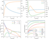 |
Fig. 2 Example model from the population synthesis set at tmax. The x-axis of each panel spans approximately 0.3 pc, or 350” assuming a cloud distant 170 pc from the observer. For the sake of clarity, this plot shows a smaller inner region of the actual computational domain. Upper left panel: Total number density radial profile (blue curve, left y-scale), cosmic-ray ionization rate ζ (orange, right y-scale). Upper right: Gas (orange) and dust (blue) temperature radial profiles (both on left y-scale), and radial velocity profile (green, right y-scale). Lower left: Cooling and heating contributions. In particular, Λd is the dust cooling, ΛCO the CO cooling, ΛZ the cooling from atomic species (C, C+, and O); instead, Γad is the adiabatic heating (i.e., compressional heating), ΓCR the cosmic-ray heating, and Γphe the dust photoelectric heating. The cooling and heating contributions below 10−26 erg s−1 cm−3 are not reported in the legend. Lower right: Radial profile of a subset of the chemical species computed with the network of 4406 reactions. The fractional abundance is relative to the total number density. COd (dashed green) is the CO on the dust surface. The comparison with Sipilä & Caselli (2018) is reported in Appendix C. |
Chemical initial conditions.
3.4 Chemical post-processing
In this work, we are interested in molecules such as DCO+, o-H2D+, N2H+, N2D+. The modeling of their evolution requires a more comprehensive network than the one in Sect. 3.3. To this end, we employed the network described in Bovino et al. (2020) that includes 4406 reactions and 136 chemical species (see Appendix B).
The chemical initial conditions employed for this network are reported in Table 1, labeled as large and both. For H2, we assume an initial fractional abundance of 0.5 and an ortho-to-para ratio of 10−3 (Pagani et al. 2013; Lupi et al. 2021). As mentioned in the previous section, the initial conditions are arbitrary and play a major role in the chemical evolution of the pre-stellar model. However, for the aims of the present paper, we do not address this issue.
This post-processing approach allows the evolution of the complex network to be locally independent of temperature evolution. In other words, the Lagrangian particle evolution temperature is time-dependent (as computed in Sect. 3.3), but we assume the chemical evolution to be at constant temperature during each timestep. This allows a much faster calculation since, at each call, the solver’s Jacobian is not influenced by temperature variations, greatly reducing the stiffness of the ordinary differential equation system. In principle, we could use KROME to evolve the temperature together with the 4406-reactions network, but this will greatly increase the computational time and create potential numerical instabilities. At the present stage, for development efficiency reasons, we prefer to focus on reducing the computational cost rather than achieving full consistency. We plan to improve the pipeline in future works.
We verified the correctness of our approach by comparing the abundance of the coolant and the colliders obtained with the two chemical networks, finding no relevant differences in the cooling functions.
In the lower right panel of Fig. 2, we show an example of some selected chemical species radial profiles, including the tracers employed later in the synthetic observations.
Parameters employed in this work.
3.5 Model parameter definition and their correlation
In Sect. 3.2, we defined some randomly sampled parameters: maximum central number density (nmax), visual extinction at the limit of the computational domain (AV,0), turbulence velocity dispersion (συ), collapse time factor (τ), and the mass of simulation domain (M). To infer additional information from our models, we define some derived parameters3. These are reported in Table 2 and evaluated at a specific arbitrary distance of 104 au. In addition, we fit the radial profile of the cosmic-ray ionization rate at t = tmax and for r ≤ 4 × 10⁴ au. We employ a four-parameter dimensionless function
![Mathematical equation: \hat{\zeta}(r') = \frac{a_0}{1+\exp\left[a_1(r' - a_2)\right]} + a_3\,,](/articles/aa/full_html/2025/10/aa53266-24/aa53266-24-eq16.png) (3)
(3)
where r′ = 0.57 [log(r/au) - 1] - 1.2 and ζ = ζ∕(10−17 s−1) - 4. The additional parameters are therefore a0, a1, a2, and a3. Despite the change of coordinates, ζ̂(r′) has the same physical interpretation and properties of ζ (r). This relation is empirically determined a posteriori from the data and has no intentional physical meaning.
Figure 3 reports the correlations and the distribution of the sampled parameters in the 3000 models. The asterisk (*) in the superscript indicates a logarithmic sample; otherwise, it is assumed to be linear. The sampling type is manually chosen to maximize the uniformity of the distribution. The panels on the diagonal of Fig. 3 show the distribution of the selected parameters. As expected, the randomized parameters are uniformly sampled, apart from συ, which is a function of the maximum radial velocity and, therefore, shows a non-uniform distribution.
Conversely, the derived parameters show some degree of correlation with the random parameters and/or between them, as they are constrained by physics. The two-dimensional histograms in the lower triangle of the matrix of panels indicate their sampling of the parameter space and their correlation. These plots already show that there are some “forbidden” combinations, for example, large dust temperature ( ) and large visual extinction (AV,0) at the same time. Analogously, in the upper triangle, we report the absolute value of the Pearson correlation algorithm coefficient for pair parameters to measure the degree of correlation. For example, AV,0 and
  strongly correlate since AV is a key factor to determine the impinging radiation on a dust grain. For the same reason, the dust temperature correlates with cosmic-ray ionization rate since ζ is scaled with the external column density, which is also proportional to AV,0. The time factor τ correlates with the chemical species with long chemical timescales, which also correlates with συ, being a fraction of the maximum radial velocity that is scaled by τ.
It is important to note that these relations are calculated at 104 au, hence, any radial effect is neglected. The dependence with the radius is included in the ai coefficients. As expected, they correlate with each other, and in particular, a0, being the scaling factor of Eq. (3), correlates with ζ1e4.
Despite most of the parameters having no radial dependence, this is implicitly present in the synthetic observations of the key chemical species, which, by construction, include information from different parts of the observed object.
4 Synthetic observations
Since we have the radial profile of the chemical composition of each model, we can produce synthetic spectral observations to mimic an observed pre-stellar core at time tmax. We then construct a spherical core based on the specific radial profile obtained by the chemical evolution. In this way, we have a 3D structure with chemical abundances, velocity, and temperature. This allows us to employ the publicly available code LOC4, which takes into account the aforementioned quantities and the turbulence velocity dispersion. LOC is an OpenCL-based tool for computing the radiative transfer modeling of molecular lines (Juvela 1997, 2020).
We designed a pipeline to automatically produce synthetic spectra for each model using the GPU implementation of the code. The molecular transitions considered are between approximately 0.2 and 4 mm as reported in Table 3, alongside their main characteristics and references. The data is further described in the EMAA5 and LAMDA6 databases. Since the large chemical network described in Sect. 3.4 does not include any oxygen isotopologs, we assume that the abundance of C18O is scaled from the CO abundance by using a constant factor 1/560 (Wilson & Rood 1994; Sipilä et al. 2022). We are aware that this approach is a simplification, and we will expand the chemical network in a future version of the code by including more isotopologs. As implemented, we expect any information we obtain on C 18O to be a property of CO. However, this value is supposed to be a valid assumption, at least in the local ISM, and, in addition, the expected oxygen fractionation is modest (Loison et al. 2019).
We use the recently modified version of LOC, which allows us to include the radial profile of the main species and the radial profiles of the various colliders. Our tests show that these recent changes do not significantly affect the results, especially for molecules with molecular hydrogen as the main collider.
We arbitrarily assumed a distance from the observer of 170pc for all the models, similarly to real observed objects (e.g., in the Taurus Molecular Cloud Complex Torres et al. 2007; Lombardi et al. 2008; Galli et al. 2019). For all the transitions, we employed a bandwidth of 4 km s−1 and 128 channels, except for the non-LTE hyperfine structure calculations of N2H+, N2D+, and HCN where the bandwidth is incremented internally by LOC to accommodate all the observable lines. In this case, the spectra have been later interpolated over a 128-channel grid in the range of the new bandwidth, obtaining a smaller velocity resolution for these molecules. The interpolation does not show any significant distortion from the original spectrum, and this remapping is not relevant to the aims of this work.
LOC produces a 2D map of the source for each velocity channel. The spectra are then convoluted with a 2D Gaussian function to mimic a telescope beam as in Table 3. To this end, we use a customized version of the LOC convolution algorithm that produces the same results as LOC, but it is more efficient for our setup. After this step, we extract the spectrum in the center of the source, obtaining a 1D function of the velocity channels.
In Fig. 4, we report an example of one of the calculated synthetic spectra. The solid lines represent the convoluted spectra after being produced by LOC. Note again that since N2H+, N2D+, and HCN are modeled with their non-LTE hyperfine structure, LOC accommodates these lines using a different velocity range than the default (−2 to 2 km s−1). At this stage, we do not include any instrumental noise, hence the information is degraded only by the assumed telescope beam. We add some noise in the next step.
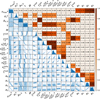 |
Fig. 3 Correlation matrix between the parameters of the models. The panels in the upper left triangle show the Pearson correlation coefficient, color-coded as indicated by the color bar. The plots in the lower right triangle show the 2D correlation histograms of the parameters of the 3000 generated models. The panels in the diagonal represent the histogram of the parameter distribution. The correlation for quantities flagged with “*” is computed using their logarithm. We note that the color bar is clipped to 0.2 to enhance the stronger correlations. |
5 Backward emulation: From observations to models
The pipeline described so far can be interpreted as a “forward” operator F that produces spectra s from a set of parameters p (i.e., s = F(p)). In our case, evaluating F takes a few minutes per parameters grid point. To reduce the computational cost, the emulators allow the behavior of complicated (thermo)chemical systems to be mimicked, greatly reducing the time spent in evaluating the output (see, e.g., Grassi et al. 2011; Holdship et al. 2021 ; Grassi et al. 2022; Smirnov-Pinchukov et al. 2022; Palud et al. 2023; Sulzer & Buck 2023; Asensio Ramos et al. 2024; Branca & Pallottini 2024; Maes et al. 2024). An additional and relevant advantage of the reduced computational cost is the capability to quickly evaluate how input perturbations propagate to the output solution (Heyl et al. 2023).
However, rather than evaluating F, our aim is to understand how the information is degraded in this process, and in particular, how s can be employed to reconstruct p. We therefore need to design the inverse (“backward”) operator B = F−1, so that p = B(s). Analogously to the forward case, we take advantage of emulation to invert the problem and later analyze how variations of s have an effect on p.
Although there are established techniques to reconstruct some of the core parameters from some specific spectral information (e.g., determining ζ from HCO+, DCO+, and other chemical tracers, as described in Caselli et al. 1998 or Bovino et al. 2020), in our case, we use a blind approach that employs all the spectra, all the channels, and all the parameters at the same time. In particular, we emulate the backward operator with a neural network (NN) that will “learn” to predict p from s.
Following a standard machine learning procedure, we divided our set of 3000 models into a training (2100 models), a validation (450), and a test set (450). The training set is used to train the NN, the validation set is used to determine if we are overfitting or underfitting our data while training, and the test set is used to verify our predictions on “new” data. We visually verified that the distributions of each parameter in the sets are relatively uniform without performing any specific analysis, for example, to verify if some models in the test set are outside the convex hull of the training and validation set input features (Yousefzadeh 2021).
We normalize each transition (i.e., the input data) in the [−1,1] range between zero and the maximum temperature of the whole set. For example, the transition 1-0 of HCO+ is normalized considering the maximum value of the given transition in all the training, validation, and test set models. This might overestimate the transitions with small maximum values (e.g., p-H2D+). To avoid this, we introduce some Gaussian noise with a 10 mK dispersion, eliminating all the information below this temperature threshold. We use the same noise for each molecule to avoid the NN recognizing the level of noise rather than the actual features of the emitted lines.
To reduce the computational impact, in particular the memory usage, we remove some of the transitions that we know are less relevant to our problem (e.g., the p-H2D+ signal is smaller than the noise we introduced). We remove C18O being its abundance a scaling of CO, but also as a test to determine if the remaining transitions are capable of inferring C18O and CO information even without the specific molecular lines. We also remove some additional transitions to simplify the final interpretation output, for example, HCO+ (2-1). The final lines are DCO+ (1-0, 3-2), HCN (1-0), HCO+ (1-0, 3-2), N2D+ (1-0, 3-2), N2H+ (1-0, 3-2), and o-H2D+ (1-0), as shown in the last column of Table 3. This corresponds to 1280 velocity channels (i.e., 1280 input features in the NN).
We normalize the parameters in Table 2 (i.e., the output data) in the [−1,1] range, using the logarithmic values of nmax, συ, and the abundances at r = 104 au of C18O, HCO+, and DCO+, while the actual value for the other parameters. This choice maximizes the uniformity of the distribution. We have 18 parameters (i.e., 18 output features) in the NN.
The NN is composed of 3 fully connected hidden layers of 64, 32, and 16 neurons each. The activation between each layer is a ReLU function, apart from the last two (i.e., the last hidden layer and output layer), which are directly connected. The code is implemented in Pytorch7, using an MSE loss function and an Adam optimizer with a learning rate of 10−3. All the other parameters follow the Pytorch default.
The NN architecture is designed to mimic an (auto)encoder in order to have a rough estimate of the information compression via dimensionality reduction (Ballard 1987; Champion et al. 2019; Grassi et al. 2022). The specific number of dimensions is empirically determined by verifying the test set predictions while reducing the number of hidden neurons at every training attempt. We do not use any hyper-parameter optimization (Yu & Zhu 2020).
The number of neurons in the first hidden layer is compatible with the PCA8 of the input data set, where 99.99% of the variance is explained by 69 components (cf. Palud et al. 2023). Analogous consideration can be made for the last hidden layer, which is smaller than the output layer. Even in this case, increasing the size of the last hidden layer does not affect our results.
We stop the training after 104 epochs to avoid overfitting, as shown by the total training and validation losses in Fig. 5. The noise in both losses is produced by the individual losses of some specific parameters, like the total mass (M) or the dust temperature at 104 au ( ). Analogusly, the turbulence velocity dispersion (συ) and the total mass (M) prevent the total loss from becoming constant (while we have verified that all the other individual losses become constant after a few thousand epochs). Some strategies could improve this behavior: we can use an NN for each physical parameter, add weights in the MSE terms to reduce or increase the efficiency of the “correction” of a specific parameter, or change the parameters of the optimizer (e.g., the learning rate). However, at this stage, we do not optimize the training to keep the method as generic as possible.
To better assess the error for each parameter, we compare the predictions of the NN using the models in the test set. The result is the scatter plot in Fig. 6. The dashed line in each panel represents the perfect match between true and predicted values, while the dotted line is the fit of the scatter plot points. Ideally, all the points should lie on the dashed line. We added the contours calculated using a Gaussian Kernel Density Estimation (KDE) algorithm (using the Scott method for the bandwidth estimator, Scott 1992) to provide a statistical overview of the results. The KDE represents the probability distribution of the data points.
We note that most quantities are well-reproduced by the NN, apart from συ and M. This indicates that the spectra retain the information on most of the model parameters. As a proof of concept, we applied the same procedure by adding a Gaussian noise of 5 K to the spectra (i.e., comparable to the highest intensities found). In this case, the NN fails to reproduce every parameter. For a similar reason, as shown by the συ panel in Fig. 6, the NN fails to predict very small velocity dispersions (i.e., it cannot determine συ below a certain threshold).
It is worth noticing that although the NN fails to reproduce συ and M, this does not necessarily mean that the spectra do not retain the information on these parameters. In fact, the reason could be a standard NN failure in learning the connection between input and output (see the discussion on the loss above). This issue could be further explored by the use of mutual information as discussed by Einig et al. (2024). On the other hand, an accurate NN parameter reproduction indicates that the spectra actually retain the information (sufficient condition).
To quantify the error, we follow a procedure similar to Palud et al. (2023) by comparing for each parameter the statistical properties of the relative error distribution in the linear space. By calculating the median and the maximum from each error distribution, we found that the medians of all the quantities are below 5%, apart from nmax,  , and a2, that are around 10%, and a3 and συ that are around the 100%. The best-reproduced quantity is ζ1e4 with a median around 0.7%. The maximum error in some cases reaches 50% (the molecular abundances, τ, and nmax), while it is generally around the 20%, if we exclude again a3 and συ. However, it is important to notice that a single isolated outlier test model causes the maximum error, and the 90th percentile of each error distribution is always well below this maximum error. Furthermore, although the relative error gives a good estimate of the NN performance, we remark that the accuracy depends on each quantity’s physical meaning and the desired precision for the specific scientific problem. In our case, for example, to verify the NN prediction on ai, we compare the predicted and expected Eq. (3) for the models in the test set, finding a negligible error (well below 5 × 10⁻¹⁸ s−1), as discussed in more detail in Appendix E. Therefore, in an ideal set-up, the NN loss for the ai values should be defined on the precision required by Eq. (3).
The analysis presented in this section only tells us whether the parameters are well-reproduced, while in Sect. 6, by analyzing the corresponding spectra, we investigate which emission line plays a role in determining the final parameter values. The forward emulator is discussed in Appendix D.
Molecules employed in this work and their transitions.
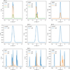 |
Fig. 4 Example spectra for the model in Fig. 2. Each panel reports the spectra of the molecule and the transitions indicated in the legend. The spectra are convoluted with a telescope beam, as discussed in the main text. We note that the y-axis is scaled to the value at the top of the panel, e.g., C18O temperature is scaled to 10−1. All the spectra are calculated with a −2 to +2 km s−1 bandwidth range and 128 channels, except for N2H+, N2D+, and HCN where the bandwidth is calculated by LOC to take into account the hyperfine structure of these molecules, but interpolated to use 128 channels. We also use the spectra centered according to the LOC output (i.e., the position of 0kms−1). |
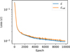 |
Fig. 5 Training (blue) and validation (orange) total loss at different epochs for the backward emulation training. Although the total loss does not become constant, we note that the individual losses of the physical parameters (not reported here) become constant after a few epochs, apart from the turbulence velocity dispersion (συ) and the total mass (M) that drive the total loss. |
6 Results of the SHAP analysis
The advantage of an NN-based accurate predictor is not only the capability of inverting the original pipeline but also the extremely small computational cost and the differentiability of the output features with respect to the input features. For this reason, the NN allows a large number of evaluations so that we can explore how the input (the spectra) affects the output (the parameters). To this end, we employed the SHapley Additive exPlanations9 (SHAP), which connects optimal credit allocation with local explanations using the classical Shapley values from game theory and their related extensions (Lundberg & Lee 2017). More in detail, this cooperative game theory concept provides a fair distribution of the prediction to the input data depending on their contribution to the global prediction. To calculate the SHAP value for a specific input feature (in our case, a spectral velocity channel), we compute the average marginal contribution of that channel across all possible combinations of channels. This considers the importance of the input channel both alone and in all possible combinations.
We employed the class DeepExplainer of SHAP, based on DeepLIFT (Shrikumar et al. 2017), that approximates the conditional expectations of SHAP values using a selection of background samples. We note that DeepExplainer effectively provides local feature contributions for specific predictions, but it does not meet the criteria for global sensitivity analysis, which requires evaluating input impact across the entire input space (Saltelli et al. 2019). We apply this method to each parameter independently using the models in the training set to determine the channels’ contributions to the prediction of that specific parameter. The SHAP values are then evaluated on the test set.
This analysis allows us to produce a figure similar to Fig. 7 for each parameter. The large left panel shows a colormap of the SHAP values of the test set models. On the x-axis, we have the velocity channels, while on the y-axis, the parameter value of the given test set. To compute the numbers distributed over the left panel, we average each channel’s SHAP values and take the maximum. In this way, we have the maximum average contribution of the given transition in the range of parameter values between the two horizontal solid lines. For the sake of clarity, if the absolute value of the maximum is above 0.03, we render the number with a larger font and a bounding box. Otherwise, the numbers are represented with a smaller font. The font color indicates the positive (red) and negative values (blue). In the right small panels, we have the spectra of some selected models corresponding to the positions indicated by the arrows outside the left panel. The position of the arrow marks the exact value on the y-axis and corresponds to the text in the top left corner of each panel on the right.
From this figure, we find that the 3-2 transition of N2H+ and both transitions of N2D+ (3-2 more than 1-0) are the key contributors to the value of the cosmic-ray ionization rate at 104 au (ζ1e4). The sign of the average SHAP value indicates the positive or negative contribution to the parameter, for example a large value of the N2H+ (3-2) transition produces high values of ζ1e4 (positive values), and vice-versa. This behavior corresponds to the right panels, where the peak of N2H+ (3-2) spectrum scales proportionally to ζ1e4.
The SHAP analysis also indicates which parts of the spectrum contribute to the final value. For example, N2H+ (3-2) has a broader vertical strip of SHAP values in the left panel, when compared to N2D+ (3-2); Analogously, HCN contributes with all the three hyperfine lines, N2D+ (1-0) with two lines, and o-H2D+ with the “sides” of the spectral line, suggesting that the width of the line plays a role in the final result. However, the contributions of these two molecules are negligible, meaning that their presence is only needed to fine-tune the NN prediction.
Conversely, HCO+ seems to play a minor role. However, from Caselli et al. (1998), we know that HCO+ and DCO+ are powerful indicators of the cosmic-ray ionization rate. This is because SHAP method is an explainer of the interpretation of the NN. The optimization found by the NN is accurate (i.e., it predicts the correct values; see Fig. 6), but it is not necessarily the most straightforward explanation10. This is clear from Fig. 8, where we plot the KDE of the maximum intensity of each transition against the expected ζ1e4 value in the test set. We note that N2H+ (3-2) correlates with the ionization rate, as suggested by the SHAP analysis. However, from Fig. 8 (last panel), the peak of o-H2D+ also seems to correlate with ζ1e4, while SHAP, from Fig. 7 (last column of the first panel), “suggests” that most of the information resides in the width of the transition rather than in the peak. Conversely, the role of N2D+ (3-2) is unclear from the KDE plot alone, while SHAP gives this further insight.
The NN allows us to determine single quantities, such as ζ1e4, but also multiple components at once from the observations, like predicting the four coefficients ai of the fit we described in Eq. (3). Here, the interpretation is more complicated since several transitions play a different role for different coefficients and different coefficient values. As an explanatory case, we discuss a0, which represents the scaling of the fitting function, and hence, it is immediately connected to the average value of cosmic-ray ionization rate. We note from Fig. 9 that a0 is affected by N2D+ (3-2) in a similar way to ζ1e4. However, other molecules (DCO+, HCN, N2H+, and o-H2D+) are also involved in determining a0, especially closer to its upper and lower values. Analogously, the other coefficients present similar complex interplay patterns, especially a1, which also has the largest uncertainty, being the scaling factor in the argument of an exponential function. The importance of this machine learning-based analysis is also suggested by Fig. F.1, where a1 does not show any obvious correlation with the peaks of the lines.
In addition, using the NN could give information on quantities that are not derivable from the observation alone. For example, C18O at 104 au ( ) is well-reproduced by the NN, although we do not include any C18O emission line in the input of the NN, thus suggesting that the other lines can fairly predict it. In this case, the SHAP analysis (Fig. F.2) indicates that N2D+ (1-0), HCO+ (1-0), and HCN retain the information necessary for the NN to reconstruct the abundance of C18O. If we compare this result with the KDE distribution of the peaks of the lines (Fig. F.3), we note that in this case, there is no clear trend to determine C18O, indicating that is the combined information from all the lines that is used to predict the result. The prediction of C18O is possible because these species are interconnected, both directly (e.g., HCO+ is a key component of the CO formation network) and indirectly (i.e., similar physical parameters have the same impact on different molecules). However, we note that in our chemical network, the abundance of C18O is scaled from that of CO, suggesting that actual information is related to CO rather than C18O.
We finally discuss the collapse time factor (τ), which is strictly linked to the chemical timescale of the slow-evolving species, for example, HCN (Fig. F.4). The abundance of this species depends on the initial conditions (i.e., N and N2) and on the temporal evolution. Since, in our case, the initial conditions are fixed, if we allow a slower collapse (larger τ), HCN is destroyed more rapidly, as indicated by the weakening of the lines in the right panels. A similar behavior is shown by N2D+, which increases its abundance when longer times favor the conversion from N2H+.
In principle, it is possible to perform this analysis on every parameter and employ additional parameters not included at this stage (e.g., specify quantities at different radii than 104 au, or define fitting functions similar to Eq. (3)). However, for the aims of the present work, we limit our analysis to the aforementioned quantities.
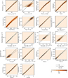 |
Fig. 6 Comparison between the true (x-axis) and the predicted (y-axis) parameter values for the models in the test set (scatter plot points). Each panel is calculated for a specific model parameter (see axis labels). A perfect match between the true and predicted values corresponds to the dashed line. The dotted line represents the fit of the scatter points, while the colored contours are their kernel density estimation (KDE) normalized to the maximum value. The KDE color scale in the last panel is the same for all the panels. We note that (ζ) is in units of 10−17 s−1. |
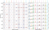 |
Fig. 7 Left panel: Colormap of the SHAP values for each channel and each ζ1e4 value in the test set. The numbers indicate the average of the SHAP value in the given part of the plot. The numbers with bounding boxes have an absolute value larger than 0.03. Right panels: Spectra corresponding to the model at the ζ1e4 value indicated by the arrow (and reported in the upper left part of each panel). For the sake of clarity, the temperature is normalized to the maximum of each transition (similarly to the NN input data normalization). Each color corresponds to a different molecular transition, as labeled at the top. The labels also indicate the correspondence between the channels in the left and right panels. |
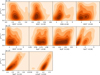 |
Fig. 8 Kernel density estimation of the peak value of the spectrum for each transition (one per panel, see x-axis label) and the ζ1 e4 of the corresponding model (see y-axis label). We note the scaling factor for the y-axis (1e-17), and the varying range of the x-axis. The parameters of the KDE algorithm are the same as in Fig. 6. |
7 Limitations
Models are limited by definition. The choice of the 1D profile not only limits the modeling of any geometrical asymmetry but does not allow the inclusion of any magnetic field. In this regard, the choice of parameterizing the presence of magnetic fields with τ does not completely solve the problem and limits the interpretability of the collapse dynamics. Even with additional physics, it is important to remark that the Larson collapse is a simplified approach with respect to the observed dynamics (Keto et al. 2015; Vaytet & Haugbølle 2017).
Computing the hydrodynamics in the isothermal case first and then computing the temperature on top of the tracer particles is another assumption that might exclude any complex interplay between hydrodynamics and thermochemical evolution. However, the temperature range we found suggests that within this context this interplay is limited. Despite the use of tracer particles, which removes the issue of chemical species advection, post-processing might produce inaccurate results due to the lack of self-consistency (Ferrada-Chamorro et al. 2021). However, there are successful cases where it is consistently employed (e.g., Panessa et al. 2023).
Although the “large” chemical network contains 136 chemical species, it does not include several species that might play a role in the synthetic observations or in the chemical evolution, such as ammonia or C18O (Sipilä et al. 2022). In addition, we limit our analysis to fixed initial chemical conditions, but some slowing-evolving species like HCN depend on the specific initial conditions (Hily-Blant et al. 2010). Similarly, some of the correlations found or some of the observed features might be produced by non-chemical correlations generated by some inaccurate chemical rate, missing chemical pathway, or timedependent effect enhanced by the inaccurate initial conditions. In general, synthetic observations observe the modeled chemical network rather than an actual astrophysical object. Therefore, they should be interpreted carefully, especially when large and complex chemical networks are involved, and multiple species are observed simultaneously.
A comprehensive review of the techniques to link observations and physical quantities is beyond the aims of the present paper. Therefore, we limit our summary to some of the standard and well-established implementations that include best model parameter grid search based on metric minimization of observed and simulated quantities (e.g., Sheffer et al. 2011; Joblin et al. 2018 and Wu et al. 2018), and methods that do not rely on precomputed grids, such as gradient descent with various algorithms (e.g., Galliano et al. 2003; Marchal et al. 2019, and Paumard et al. 2022), Bayesian-based model selection (e.g., Zucker et al. 2021; Chevallard & Charlot 2016; Jóhannesson et al. 2016 and Behrens et al. 2022), and Monte Carlo sampling with a large variety of implementations (e.g., Chevallard et al. 2013; Makrymallis & Viti 2014; Gratier et al. 2016; Galliano 2018; Holdship et al. 2018; Galliano et al. 2021 and Ramambason et al. 2022).
We do not review the advantages and limitations of each technique here due to the problem’s specific details, the astrophysical object(s) of interest, the physical model developments, and the technical implementations of the various methodologies. We merely point out that some of these techniques are capable of producing estimates of uncertainty, unlike our method (at least at the present stage). Furthermore, a common disadvantage is the intrinsic parameter degeneracy that limits all the aforementioned techniques, including the one presented in this paper. In our case, the forward operator (i.e., stages 1-6 in Fig. 1) is not necessarily invertible, so the parameters’ degeneracy might limit the optimization of the NN. In addition, if newer transitions are available or some are missing, the NN requires additional training that might not necessarily converge. On the other hand, in addition to the differentiability and the seamless interface with the SHAP architecture, the use of an NN presents some advantages, such as a training stage of a couple of minutes on a standard GPU and a negligible evaluation time, making this technique extremely effective and flexible.
To further discuss the limitations, we present an application to the pre-stellar core L1544. However, we recall that some technical aspects currently limit the applicability, and they can be addressed in the future. As we discussed earlier, emulators and NN are limited to a specific feature domain, and their application to real observations might produce false correlations or emulator hallucinations. In principle, it is possible to use the backward model F−1 to determine the physical characteristics of an observed object. In the case of the pre-stellar core L1544, the transitions observed cover several molecules available in our model, in particular, DCO+ (1-0, 3-2, Redaelli et al. 2019), HCN (1-0, Hily-Blant et al. 2010), HCO+ (1-0, 3-2, Redaelli et al. 2022), N2D+ (1-0, 3-2, Redaelli et al. 2019), N2H+ (1-0, 3-2, Redaelli et al. 2019), and o-H2D+ (1-0, Caselli et al. 2003; Vastel et al. 2006). We interpolate the observed line profiles to the channels we used in the training set, assuming zero intensity outside. However, some discrepancies exist between the simulated model and the observed quantities. The most relevant is underestimating of C18O and DCO+ line intensities. In addition, the models with the largest intensities of C18O show a double peak, which is absent in the case of L1544 (see also Keto et al. 2015 showing that quasi-equilibrium contraction is needed to reproduce the C18O and H2O lines in L1544, while Larson-Penston and singular isothermal sphere models fail). Additionally, our implementation might fail on L1544 because the NN is not trained with a consistent noise model. However, we need more tests to verify whether this issue is relevant in this context.
With these premises, the reason why we do not obtain reliable results at this stage, is mainly the presence of unexpected features in the input spectra. This artificially enhances or decreases some input nodes that generate anomalous output. The results are also influenced by the fact that probably none of the generated models resemble L1544, or that, given the complexity of our pipeline, any of the ingredients might determine an NN hallucination. However, despite the limited results, the approach of using a backward emulator is still promising, also considering different NN architectures that might be more appropriate for spectral data, like convolutional neural networks (Kiranyaz et al. 2021), and transformers (Leung & Bovy 2024; Zhang et al. 2024). Another approach could be to provide the NN with the actual fitting parameters of the lines using standard methods instead of the raw spectra (e.g., Ginsburg et al. 2022).
8 Conclusions
In this work we proposed a pipeline to connect the information in 1D hydrodynamical models of pre-stellar cores with the observed features of their synthetic spectra. This procedure employs 3000 models of hydrodynamical gravitational collapse with time-dependent thermochemistry, isotopolog chemistry, and consistent cosmic-ray propagation. We used SHAP, an interpretable machine learning technique, to connect the models’ parameters and the corresponding generated synthetic spectra.
The main findings are the following:
Most of the information is retained by the spectra, apart from the small turbulence velocity dispersion (συ) and the initial total mass (M);
SHAP, when applied to synthetic observations, represents a valid tool to explore how spectral features are connected to model parameters;
Within the assumptions of our model, cosmic rays are well reproduced. Their ionization rate at a distance of 104 au is retrieved mainly by N2H+ and N2D+, while the radial profile ζ(r) is determined by a mix of the contributions of N2D+, DCO+, HCN, N2H+, and o-H2D+;
This method is capable of obtaining information on the chemistry of molecules not included in the spectra. To this end, we removed C18O from the spectra. We found that a combination of N2D+, HCO+, and HCN can be used to constrain the abundance of C18O at 104 au;
The effects of the time dependence, namely the collapse slowing factor τ, emerge in the features of the HCN spectra, which have a relatively slow chemical timescale;
Future work is required to address the role of model uncertainties, neural network limitations, and backward emulation applied to real observations.
Acknowledgements
We thank the referee, Pierre Palud, for improving the quality of the paper. We thank Mika Juvela for the LOC update to include radially-dependent collider abundances. We thank Johannes Heyl for suggesting using DeepExplainer instead of KernelExplainer. This research was supported by the Excellence Cluster ORIGINS, funded by the Deutsche Forschungsgemeinschaft (DFG, German Research Foundation) under Germany’s Excellence Strategy - EXC-2094 - 390783311. DG acknowledges support from the INAF minigrant PACIFISM. SB acknowledges BASAL Centro de Astrofisica y Tecnologías Afines (CATA), project number AFB-17002. SB acknowledges BASAL Centro de Astrofisica y Tecnologías Afines (CATA), project number AFB-17002. This research has made use of spectroscopic and collisional data from the EMAA database (https://emaa.osug.fr and https://dx.doi.org/10.17178/EMAA).
Appendix A Chemical species included in the small chemical network
The small chemical network includes the following chemical species: e−, H, H+ H−, He, He+, He++, C, C+, C−, O, O+, O−, H2, H2+, H3+, OH, OH+, CH, CH+, CH2, CH2+, CH3+, H2O, H2O+, H2Od HCO, HCO+, HOC+, CO, CO+, COd, O2, O2+, C2, and H3O+, where the subscript “d” indicates the species on ice. We employed the rate coefficients taken from de Jong (1972); Aldrovandi & Pequignot (1973); Poulaert et al. (1978); Karpas et al. (1979); Mitchell & Deveau (1983); Lepp & Shull (1983); Janev et al. (1987); Ferland et al. (1992); Verner et al. (1996); Abel et al. (1997); Savin et al. (2004); Yoshida et al. (2006); Harada et al. (2010); Kreckel et al. (2010); Grassi et al. (2011); Forrey (2013); Stenrup et al. (2009); O’Connor et al. (2015); Wakelam et al. (2015); Millar et al. (2024). More details in Glover et al. (2010) and in the KROME network file react_CO_thin_ice, commit 6a762de.
Appendix B Chemical species included in the large chemical network
The large chemical network includes: e−, H, H+, H−, D, D+, D−, o-H2, p-H2, o-H2+, p-H2+, HD, HD+, o-H3+, p-H3+, He, He+, o-D2, p-D2, o-D2+, p-D2+, o-H2D+, p-H2D+, HeH+, o-D2H+, p-D2H+, m-D3+, o-D3+, p-D3+, C, C+, C−, CH, CH+, Nd, N, N+, CD, CD+, CH2, CH2+, NH, NH+, CHD, CHD+, Od, O, O+, O−, ND, ND+, o-NH2, p-NH2, o-NH2+, p-NH2+, CD2, CD2+, OH, OH+, OH−, NHD, NHD+, OD, OD+, OD−, o-H2O, p-H2O, o-H2O+, p-H2O+, o-ND2, p-ND2, o-ND2+, p-ND2+, HDO, HDO+, o-D2O, p-D2O, o-D2O+, p-D2O+, C2, C2+, C2H+, CN, CN+, CN−, C2D+, HCN, HNC, HCN+, HNC+, COd, CO, CO+, N2 d, N2, N2+, DNC, DCN, DNC+, DCN+, HCO, HCO+, HOC+, N2H+, NO, NO+, DCO, DOC+, DCO+, N2D+, HNO, HNO+, O2, O2+, DNO, DNO+, O2H, HO2+, O2D, DO2+, C3, C3+, C2N+, CNC+, CCO, C2O+, OCN, NCO+, CO2, CO2+, N2O, NO2, NO2+, GRAIN, GRAIN+, and GRAIN−, where o-, p-, and m-, indicate the ortho-, para-, and meta- spin states, respectively. For further details on the network, we refer to Bovino et al. (2020).
Appendix C Model comparison
In Fig. C.1, we compare the radial profiles of various quantities in our models to Sipilä & Caselli (2018) (gas temperature T, dust temperature Td, density n, and υr radial velocity). The main differences in gas temperature (T) are due to different assumptions on the heating of cosmic rays (where we use Glassgold et al. 2012 implementation and variable cosmic-ray ionization rate), and CO cooling (where we employed a custom look-up table from Omukai et al. 2010), while Sipilä & Caselli (2018) use Juvela (1997). In addition, the size of the computational domain plays a role in determining the CO column density. The difference in dust temperature (Td) is produced by a different assumption on the grain optical properties and again on the limit of the computational domain. The radial velocity (υr) is statistically smaller due to the arbitrary scaling of the collapse time factor (τ). These differences do not significantly influence the main findings and the method description.
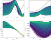 |
Fig. C.1 Radial profiles for different quantities (gas temperature T, dust temperature Td, density n, and radial velocity υr) as density probability of our models’ sample (color plot), compared with Fig. 3 of Sipilä et al. (2022), at t = 7.19 × 10⁵ yr (dashed lines). The probability density is vertically normalized to have the same integral value (i.e., unity) at each radius. We note the log-scaled radius. |
Appendix D Forward emulation: From models to observations
Analogously to the backward emulation, we trained an NN that predicts the observed spectra from the model parameters (i.e., a s = F(p) emulator). This allows us to generate spectra extremely fast by simply specifying arbitrary parameters.
In this case, the NN architecture is a fully connected feedforward consisting of two hidden layers (64 and 32 neurons). Each hidden layer has a ReLU activation function. The NN is optimized via an Adam optimizer with a learning rate of 10−3, and the mean squared error (MSE) loss function is utilized to compute the loss. The other options are the default PYTORCH options. We trained the network for 6000 epochs.
With respect to the previous method, the training efficiency is now very high, and all the line features are well-reproduced, even in the test set. This behavior is due to the lack of large degeneracies in the forward model.
After the training, it is possible to use the NN to predict any combination of values, including the non-physical ones (i.e., exploring the no data parts (in white) in the histograms) of the lower left triangle of the matrix of plots in Fig. 3. For example, the NN can produce all the spectra for a hypothetical model with a small value of the visual extinction at the limits of the computational domain (Av,0) and a small dust temperature at 104 au ( ). Our model does not achieve this combination for physical reasons (i.e., high AV,0 means insufficient radiation to heat the dust grains, hence a smaller
  ).
).
This approach is usually not recommended even if, in some cases, this “extrapolative” technique could lead to alluring physical interpretations. In fact, as a cautionary tale, reducing τ below the limits first produces a physical reduction of the HCN emission (being the HCN abundance relatively time-dependent), but then generates unphysical HCN absorption lines (NN hallucinations), which are never present in the training set (nor in the validation or test sets). For this reason, we limit our discussion to the backward “observation to model” NN.
Appendix E Cosmic-ray fit prediction error
To quantify the error of the NN in predicting a0, a1, a2, and a3, for each test model, we compute max  , where the first term is the actual Eq. (3) and the second is the same equation but using the predicted ai coefficients. The error probability density distribution is reported in Fig. E.1. The mean, the median, and the 25 and 75 quartiles are respectively indicated with dashed, dotted, and solid lines. The plot shows that the error is well below 5 × 10⁻¹⁸ s−1.
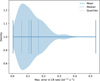 |
Fig. E.1 Density probability of the maximum error of predicting ζ(r) with NN. The mean, the median, and the 25 and 75 quartiles are respectively indicated as dashed, dotted, and solid lines. |
Appendix F Additional figures
This section contains the additional figures moved here upon editorial request. The figures are discussed in the main text. Figure F.1 is the KDE of the peak value of the spectrum for each transition for the parameter a1, Fig. F.2 is the SHAP analysis for C18O, while Figs. F.3 and F.4 are the correspondent figures for C18O and the time factor τ.


References
- Abel, T., Anninos, P., Zhang, Y., & Norman, M. L. 1997, New A, 2, 181 [NASA ADS] [CrossRef] [Google Scholar]
- Aldrovandi, S. M. V., & Pequignot, D. 1973, A&A, 25, 137 [NASA ADS] [Google Scholar]
- Asensio Ramos, A., Westendorp Plaza, C., Navarro-Almaida, D., et al. 2024, MNRAS, 531, 4930 [NASA ADS] [CrossRef] [Google Scholar]
- Bakes, E. L. O., & Tielens, A. G. G. M. 1994, ApJ, 427, 822 [NASA ADS] [CrossRef] [Google Scholar]
- Ballard, D. H. 1987, in Proceedings of the Sixth National Conference on Artificial Intelligence, 1, AAAI’87 (AAAI Press), 279 [Google Scholar]
- Behrens, E., Mangum, J. G., Holdship, J., et al. 2022, ApJ, 939, 119 [NASA ADS] [CrossRef] [Google Scholar]
- Behrens, E., Mangum, J. G., Viti, S., et al. 2024, ApJ, 977, 38 [Google Scholar]
- Bergin, E. A., Maret, S., & van der Tak, F. 2005, in ESA Special Publication, 577, ed. A. Wilson, 185 [Google Scholar]
- Bovino, S., Ferrada-Chamorro, S., Lupi, A., et al. 2019, ApJ, 887, 224 [NASA ADS] [CrossRef] [Google Scholar]
- Bovino, S., Ferrada-Chamorro, S., Lupi, A., Schleicher, D. R. G., & Caselli, P. 2020, MNRAS, 495, L7 [Google Scholar]
- Bovino, S., Lupi, A., Giannetti, A., et al. 2021, A&A, 654, A34 [NASA ADS] [CrossRef] [EDP Sciences] [Google Scholar]
- Branca, L., & Pallottini, A. 2024, A&A, 684, A203 [NASA ADS] [CrossRef] [EDP Sciences] [Google Scholar]
- Caselli, P. 2011, in IAU Symposium, 280, The Molecular Universe, eds. J. Cer-nicharo, & R. Bachiller, 19 [Google Scholar]
- Caselli, P., Walmsley, C. M., Terzieva, R., & Herbst, E. 1998, ApJ, 499, 234 [Google Scholar]
- Caselli, P., Walmsley, C. M., Zucconi, A., et al. 2002, ApJ, 565, 331 [NASA ADS] [CrossRef] [Google Scholar]
- Caselli, P., van der Tak, F. F. S., Ceccarelli, C., & Bacmann, A. 2003, A&A, 403, L37 [CrossRef] [EDP Sciences] [Google Scholar]
- Cen, R. 1992, ApJS, 78, 341 [NASA ADS] [CrossRef] [Google Scholar]
- Champion, K., Lusch, B., Kutz, J. N., & Brunton, S. L. 2019, PNAS, 116, 22445 [Google Scholar]
- Chevallard, J., & Charlot, S. 2016, MNRAS, 462, 1415 [NASA ADS] [CrossRef] [Google Scholar]
- Chevallard, J., Charlot, S., Wandelt, B., & Wild, V. 2013, MNRAS, 432, 2061 [CrossRef] [Google Scholar]
- Crapsi, A., Caselli, P., Walmsley, M. C., & Tafalla, M. 2007, A&A, 470, 221 [NASA ADS] [CrossRef] [EDP Sciences] [Google Scholar]
- de Jong, T. 1972, A&A, 20, 263 [NASA ADS] [Google Scholar]
- Denis-Alpizar, O., Stoecklin, T., Dutrey, A., & Guilloteau, S. 2020, MNRAS, 497, 4276 [Google Scholar]
- Diop, A., Cleeves, L. I., Anderson, D. E., Pegues, J., & Plunkett, A. 2024, ApJ, 962, 90 [Google Scholar]
- Draine, B. T. 1978, ApJS, 36, 595 [Google Scholar]
- Draine, B. T. 2003, ARA&A, 41, 241 [NASA ADS] [CrossRef] [Google Scholar]
- Draine, B. T., & Bertoldi, F. 1996, ApJ, 468, 269 [Google Scholar]
- Dumouchel, F., Faure, A., & Lique, F. 2010, MNRAS, 406, 2488 [NASA ADS] [CrossRef] [Google Scholar]
- Einig, L., Palud, P., Roueff, A., et al. 2024, A&A, 691, A109 [NASA ADS] [CrossRef] [EDP Sciences] [Google Scholar]
- Faure, A., Varambhia, H. N., Stoecklin, T., & Tennyson, J. 2007, MNRAS, 382, 840 [Google Scholar]
- Ferland, G. J., Peterson, B. M., Horne, K., Welsh, W. F., & Nahar, S. N. 1992, ApJ, 387, 95 [NASA ADS] [CrossRef] [Google Scholar]
- Ferrada-Chamorro, S., Lupi, A., & Bovino, S. 2021, MNRAS, 505, 3442 [NASA ADS] [CrossRef] [Google Scholar]
- Forrey, R. C. 2013, ApJ, 773, L25 [NASA ADS] [CrossRef] [Google Scholar]
- Galli, D., & Padovani, M. 2015, in Proceedings of Cosmic Rays and the InterStellar Medium – PoS(CRISM2014), 221, 030 [Google Scholar]
- Galli, P. A. B., Loinard, L., Bouy, H., et al. 2019, A&A, 630, A137 [NASA ADS] [CrossRef] [EDP Sciences] [Google Scholar]
- Galliano, F. 2018, MNRAS, 476, 1445 [NASA ADS] [CrossRef] [Google Scholar]
- Galliano, F., Madden, S. C., Jones, A. P., et al. 2003, A&A, 407, 159 [NASA ADS] [CrossRef] [EDP Sciences] [Google Scholar]
- Galliano, F., Nersesian, A., Bianchi, S., et al. 2021, A&A, 649, A18 [EDP Sciences] [Google Scholar]
- Ginsburg, A., Sokolov, V., de Val-Borro, M., et al. 2022, AJ, 163, 291 [NASA ADS] [CrossRef] [Google Scholar]
- Glassgold, A. E., Galli, D., & Padovani, M. 2012, ApJ, 756, 157 [Google Scholar]
- Glover, S. C. O. 2015, MNRAS, 453, 2901 [Google Scholar]
- Glover, S. C. O., & Clark, P. C. 2012, MNRAS, 421, 116 [NASA ADS] [Google Scholar]
- Glover, S. C. O., Federrath, C., Mac Low, M. M., & Klessen, R. S. 2010, MNRAS, 404, 2 [Google Scholar]
- Gong, M., Ostriker, E. C., & Wolfire, M. G. 2017, ApJ, 843, 38 [NASA ADS] [CrossRef] [Google Scholar]
- Grassi, T., Krstic, P., Merlin, E., et al. 2011, A&A, 533, A123 [NASA ADS] [CrossRef] [EDP Sciences] [Google Scholar]
- Grassi, T., Merlin, E., Piovan, L., Buonomo, U., & Chiosi, C. 2011, arXiv e-prints [arXiv:1103.0509">arXiv:1103.0509] [Google Scholar]
- Grassi, T., Bovino, S., Schleicher, D. R. G., et al. 2014, MNRAS, 439, 2386 [Google Scholar]
- Grassi, T., Bovino, S., Haugbølle, T., & Schleicher, D. R. G. 2017, MNRAS, 466, 1259 [Google Scholar]
- Grassi, T., Nauman, F., Ramsey, J. P., et al. 2022, A&A, 668, A139 [NASA ADS] [CrossRef] [EDP Sciences] [Google Scholar]
- Gratier, P., Majumdar, L., Ohishi, M., et al. 2016, ApJS, 225, 25 [Google Scholar]
- Gratier, P., Pety, J., Bron, E., et al. 2021, A&A, 645, A27 [CrossRef] [EDP Sciences] [Google Scholar]
- Halko, N., Martinsson, P. G., & Tropp, J. A. 2011, SIAM Rev., 53, 217 [CrossRef] [Google Scholar]
- Harada, N., Herbst, E., & Wakelam, V. 2010, ApJ, 721, 1570 [NASA ADS] [CrossRef] [Google Scholar]
- Harju, J., Daniel, F., Sipilä, O., et al. 2017, A&A, 600, A61 [NASA ADS] [CrossRef] [EDP Sciences] [Google Scholar]
- Heyl, J., Butterworth, J., & Viti, S. 2023, MNRAS, 526, 404 [NASA ADS] [CrossRef] [Google Scholar]
- Hily-Blant, P., Walmsley, M., Pineau Des Forêts, G., & Flower, D. 2010, A&A, 513, A41 [NASA ADS] [CrossRef] [EDP Sciences] [Google Scholar]
- Holdship, J., Jeffrey, N., Makrymallis, A., Viti, S., & Yates, J. 2018, ApJ, 866, 116 [NASA ADS] [CrossRef] [Google Scholar]
- Holdship, J., Viti, S., Haworth, T. J., & Ilee, J. D. 2021, A&A, 653, A76 [NASA ADS] [CrossRef] [EDP Sciences] [Google Scholar]
- Hugo, E., Asvany, O., & Schlemmer, S. 2009, J. Chem. Phys., 130, 164302 [Google Scholar]
- Indriolo, N., & McCall, B. J. 2012, ApJ, 745, 91 [NASA ADS] [CrossRef] [Google Scholar]
- Janev, R. K., Langer, W. D., & Evans, K. 1987, Elementary Processes in Hydrogen-Helium Plasmas - Cross Sections and Reaction Rate Coefficients [Google Scholar]
- Jensen, S. S., Spezzano, S., Caselli, P., Grassi, T., & Haugbølle, T. 2023, A&A, 675, A34 [NASA ADS] [CrossRef] [EDP Sciences] [Google Scholar]
- Joblin, C., Bron, E., Pinto, C., et al. 2018, A&A, 615, A129 [NASA ADS] [CrossRef] [EDP Sciences] [Google Scholar]
- Johannesson, G., Ruiz de Austri, R., Vincent, A. C., et al. 2016, ApJ, 824, 16 [CrossRef] [Google Scholar]
- Juvela, M. 1997, A&A, 322, 943 [NASA ADS] [Google Scholar]
- Juvela, M. 2020, A&A, 644, A151 [NASA ADS] [CrossRef] [EDP Sciences] [Google Scholar]
- Karpas, Z., Anicich, V., & Huntress, W. T. 1979, J. Chem. Phys., 70, 2877 [NASA ADS] [CrossRef] [Google Scholar]
- Kaufman, M. J., Wolfire, M. G., Hollenbach, D. J., & Luhman, M. L. 1999, ApJ, 527, 795 [Google Scholar]
- Keto, E., & Caselli, P. 2008, ApJ, 683, 238 [Google Scholar]
- Keto, E., Caselli, P., & Rawlings, J. 2015, MNRAS, 446, 3731 [NASA ADS] [CrossRef] [Google Scholar]
- Kiranyaz, S., Avci, O., Abdeljaber, O., et al. 2021, Mech. Syst. Signal Process., 151, 107398 [NASA ADS] [CrossRef] [Google Scholar]
- Kong, S., Caselli, P., Tan, J. C., Wakelam, V., & Sipilä, O. 2015, ApJ, 804, 98 [NASA ADS] [CrossRef] [Google Scholar]
- Koumpia, E., Evans, L., Di Francesco, J., van der Tak, F. F. S., & Oudmaijer, R. D. 2020, A&A, 643, A61 [NASA ADS] [CrossRef] [EDP Sciences] [Google Scholar]
- Kreckel, H., Bruhns, H., Èizek, M., et al. 2010, Science, 329, 69 [NASA ADS] [CrossRef] [Google Scholar]
- Larson, R. B. 1969, MNRAS, 145, 271 [Google Scholar]
- Lepp, S., & Shull, J. M. 1983, ApJ, 270, 578 [NASA ADS] [CrossRef] [Google Scholar]
- Leung, H. W., & Bovy, J. 2024, MNRAS, 527, 1494 [Google Scholar]
- Lin, Y., Spezzano, S., Sipilä, O., Vasyunin, A., & Caselli, P. 2022, A&A, 665, A131 [NASA ADS] [CrossRef] [EDP Sciences] [Google Scholar]
- Loison, J.-C., Wakelam, V., Gratier, P., et al. 2019, MNRAS, 485, 5777 [Google Scholar]
- Lombardi, M., Lada, C. J., & Alves, J. 2008, A&A, 489, 143 [NASA ADS] [CrossRef] [EDP Sciences] [Google Scholar]
- Lundberg, S. M., & Lee, S.-I. 2017, in Advances in Neural Information Processing Systems 30, eds. I. Guyon, U. V. Luxburg, S. Bengio, et al. (Curran Associates, Inc.), 4765 [Google Scholar]
- Lupi, A., Bovino, S., & Grassi, T. 2021, A&A, 654, L6 [NASA ADS] [CrossRef] [EDP Sciences] [Google Scholar]
- Maes, S., De Ceuster, F., Van de Sande, M., & Decin, L. 2024, ApJ, 969, 79 [NASA ADS] [CrossRef] [Google Scholar]
- Maio, U., Dolag, K., Ciardi, B., & Tornatore, L. 2007, MNRAS, 379, 963 [NASA ADS] [CrossRef] [Google Scholar]
- Makrymallis, A., & Viti, S. 2014, ApJ, 794, 45 [NASA ADS] [CrossRef] [Google Scholar]
- Marchal, A., Miville-Deschênes, M.-A., Orieux, F., et al. 2019, A&A, 626, A101 [NASA ADS] [CrossRef] [EDP Sciences] [Google Scholar]
- Millar, T. J., Walsh, C., Van de Sande, M., & Markwick, A. J. 2024, A&A, 682, A109 [NASA ADS] [CrossRef] [EDP Sciences] [Google Scholar]
- Mitchell, G. F., & Deveau, T. J. 1983, ApJ, 266, 646 [Google Scholar]
- Müller, H. S., Schläder, F., Stutzki, J., & Winnewisser, G. 2005, J. Mol. Struct., 742, 215 [CrossRef] [Google Scholar]
- Neufeld, D. A., Welty, D. E., Ivlev, A. V., et al. 2024, ApJ, 973, 143 [Google Scholar]
- Obolentseva, M., Ivlev, A. V., Silsbee, K., et al. 2024, ApJ, 973, 142 [NASA ADS] [CrossRef] [Google Scholar]
- O’Connor, A. P., Urbain, X., Stützel, J., et al. 2015, ApJS, 219, 6 [Google Scholar]
- Omukai, K., Hosokawa, T., & Yoshida, N. 2010, ApJ, 722, 1793 [NASA ADS] [CrossRef] [Google Scholar]
- Ossenkopf, V., & Henning, T. 1994, A&A, 291, 943 [NASA ADS] [Google Scholar]
- Padovani, M., & Gaches, B. 2024, in Astrochemical Modeling: Practical Aspects of Microphysics in Numerical Simulations, eds. S. Bovino, & T. Grassi, 189 [Google Scholar]
- Pagani, L., Lesaffre, P., Jorfi, M., et al. 2013, A&A, 551, A38 [NASA ADS] [CrossRef] [EDP Sciences] [Google Scholar]
- Padovani, M., Ivlev, A. V., Galli, D., & Caselli, P. 2018, A&A, 614, A111 [NASA ADS] [CrossRef] [EDP Sciences] [Google Scholar]
- Palud, P., Einig, L., Le Petit, F., et al. 2023, A&A, 678, A198 [NASA ADS] [CrossRef] [EDP Sciences] [Google Scholar]
- Panessa, M., Seifried, D., Walch, S., et al. 2023, MNRAS, 523, 6138 [NASA ADS] [CrossRef] [Google Scholar]
- Paumard, T., Ciurlo, A., Morris, M. R., Do, T., & Ghez, A. M. 2022, A&A, 664, A97 [NASA ADS] [CrossRef] [EDP Sciences] [Google Scholar]
- Pedregosa, F., Varoquaux, G., Gramfort, A., et al. 2011, J. Mach. Learn. Res., 12, 2825 [Google Scholar]
- Penston, M. V. 1969, MNRAS, 144, 425 [NASA ADS] [CrossRef] [Google Scholar]
- Pety, J., Guzmán, V. V., Orkisz, J. H., et al. 2017, A&A, 599, A98 [NASA ADS] [CrossRef] [EDP Sciences] [Google Scholar]
- Pineda, J. E., Harju, J., Caselli, P., et al. 2022, AJ, 163, 294 [NASA ADS] [CrossRef] [Google Scholar]
- Poulaert, G., Brouillard, F., Claeys, W., McGowan, J. W., & Van Wassenhove, G. 1978, J. Phys. B At. Mol. Phys., 11, L671 [Google Scholar]
- Priestley, F. D., Clark, P. C., & Whitworth, A. P. 2023, MNRAS, 519, 6392 [NASA ADS] [CrossRef] [Google Scholar]
- Punanova, A., Caselli, P., Pineda, J. E., et al. 2018, A&A, 617, A27 [NASA ADS] [CrossRef] [EDP Sciences] [Google Scholar]
- Ramambason, L., Lebouteiller, V., Bik, A., et al. 2022, A&A, 667, A35 [NASA ADS] [CrossRef] [EDP Sciences] [Google Scholar]
- Redaelli, E., Bizzocchi, L., Caselli, P., et al. 2019, A&A, 629, A15 [NASA ADS] [CrossRef] [EDP Sciences] [Google Scholar]
- Redaelli, E., Bovino, S., Sanhueza, P., et al. 2022, ApJ, 936, 169 [NASA ADS] [CrossRef] [Google Scholar]
- Redaelli, E., Bovino, S., Lupi, A., et al. 2024, A&A, 685, A67 [NASA ADS] [CrossRef] [EDP Sciences] [Google Scholar]
- Richings, A. J., Schaye, J., & Oppenheimer, B. D. 2014, MNRAS, 442, 2780 [Google Scholar]
- Saltelli, A., Aleksankina, K., Becker, W., et al. 2019, Environ. Model. Softw., 114, 29 [CrossRef] [Google Scholar]
- Savin, D. W., Krstic, P. S., Haiman, Z., & Stancil, P. C. 2004, ApJ, 606, L167 [Google Scholar]
- Scott, D. 1992, Multivariate Density Estimation: Theory, Practice, and Visualization, A Wiley-Interscience Publication (Wiley) [Google Scholar]
- Sellek, A. D., Grassi, T., Picogna, G., et al. 2024, A&A, 690, A296 [NASA ADS] [CrossRef] [EDP Sciences] [Google Scholar]
- Sheffer, Y., Wolfire, M. G., Hollenbach, D. J., Kaufman, M. J., & Cordier, M. 2011, ApJ, 741, 45 [NASA ADS] [CrossRef] [Google Scholar]
- Shimajiri, Y., Kawanishi, Y., Fujita, S., et al. 2023, MNRAS, 526, 966 [Google Scholar]
- Shrikumar, A., Greenside, P., & Kundaje, A. 2017, in Proceedings of the 34th International Conference on Machine Learning, 70, ICML’ 17 (JMLR.org), 3145 [Google Scholar]
- Sipilä, O., & Caselli, P. 2018, A&A, 615, A15 [Google Scholar]
- Sipilä, O., Caselli, P., Redaelli, E., & Spezzano, S. 2022, A&A, 668, A131 [NASA ADS] [CrossRef] [EDP Sciences] [Google Scholar]
- Smirnov-Pinchukov, G. V., Molyarova, T., Semenov, D. A., et al. 2022, A&A, 666, L8 [NASA ADS] [CrossRef] [EDP Sciences] [Google Scholar]
- Spezzano, S., Caselli, P., Bizzocchi, L., Giuliano, B. M., & Lattanzi, V. 2017, A&A, 606, A82 [NASA ADS] [CrossRef] [EDP Sciences] [Google Scholar]
- Stenrup, M., Larson, Â., & Elander, N. 2009, Phys. Rev. A, 79, 012713 [Google Scholar]
- Sulzer, I., & Buck, T. 2023, arXiv e-prints [arXiv:2312.06015">arXiv:2312.06015] [Google Scholar]
- Torres, R. M., Loinard, L., Mioduszewski, A. J., & Rodríguez, L. F. 2007, ApJ, 671, 1813 [NASA ADS] [CrossRef] [Google Scholar]
- Tritsis, A., Tassis, K., & Willacy, K. 2016, MNRAS, 458, 789 [CrossRef] [Google Scholar]
- Vastel, C., Caselli, P., Ceccarelli, C., et al. 2006, ApJ, 645, 1198 [NASA ADS] [CrossRef] [Google Scholar]
- Vaytet, N., & Haugbolle, T. 2017, A&A, 598, A116 [NASA ADS] [CrossRef] [EDP Sciences] [Google Scholar]
- Vaytet, N., Audit, E., Chabrier, G., Commerçon, B., & Masson, J. 2012, A&A, 543, A60 [NASA ADS] [CrossRef] [EDP Sciences] [Google Scholar]
- Vaytet, N., Chabrier, G., Audit, E., et al. 2013, A&A, 557, A90 [NASA ADS] [CrossRef] [EDP Sciences] [Google Scholar]
- Verner, D. A., Ferland, G. J., Korista, K. T., & Yakovlev, D. G. 1996, ApJ, 465, 487 [Google Scholar]
- Visser, R., van Dishoeck, E. F., & Black, J. H. 2009, A&A, 503, 323 [NASA ADS] [CrossRef] [EDP Sciences] [Google Scholar]
- Wakelam, V., Loison, J. C., Herbst, E., et al. 2015, ApJS, 217, 20 [NASA ADS] [CrossRef] [Google Scholar]
- Wilson, T. L., & Rood, R. 1994, ARA&A, 32, 191 [Google Scholar]
- Wolfire, M. G., McKee, C. F., Hollenbach, D., & Tielens, A. G. G. M. 2003, ApJ, 587, 278 [Google Scholar]
- Wu, R., Bron, E., Onaka, T., et al. 2018, A&A, 618, A53 [NASA ADS] [CrossRef] [EDP Sciences] [Google Scholar]
- Yang, B., Stancil, P. C., Balakrishnan, N., & Forrey, R. C. 2010, ApJ, 718, 1062 [Google Scholar]
- Yoshida, N., Omukai, K., Hernquist, L., & Abel, T. 2006, ApJ, 652, 6 [NASA ADS] [CrossRef] [Google Scholar]
- Yousefzadeh, R. 2021, arXiv e-prints [arXiv:2101.09849">arXiv:2101.09849] [Google Scholar]
- Yu, T., & Zhu, H. 2020, arXiv e-prints [arXiv:2003.05689">arXiv:2003.05689] [Google Scholar]
- Zhang, M., Wu, F., Bu, Y., et al. 2024, A&A, 683, A163 [NASA ADS] [CrossRef] [EDP Sciences] [Google Scholar]
- Zucker, C., Goodman, A., Alves, J., et al. 2021, ApJ, 919, 35 [NASA ADS] [CrossRef] [Google Scholar]
The computational domain is 1.5 × 10⁵ au for each model (i.e., enough to ensure that every model has an external region unaffected by the collapse). In other words, where the initial conditions (density and velocity) are unperturbed.
https://bitbucket.org/tgrassi/krome, commit 6a762de.
Specifically, these are not “parameters” since they are derived quantities, but for the sake of simplicity, we refer to them as parameters anyway.
Version 2.0.0.
Using PCA from sklearn.decomposition with default options, version 1.0.2. (Halko et al. 2011; Pedregosa et al. 2011).
https://github.com/shap/shap, version 0.46.0.
All Tables
All Figures
|
Fig. 1 Schematic diagram of the procedure employed in this work. The top part represents the modeling steps: (1) generating the library of gravitational collapse models; (2) randomly selecting the base models depending on the global parameters; (3) evolving the thermochemistry in the collapse model; (4) including additional chemistry with post-processing; (5) obtaining the derived quantities (e.g., the abundances of some key species); and (6) producing the synthetic spectra. The middle part is the emulation: (7a) forward emulation, from parameters to spectra; (7) backward emulation, from spectra to parameters. The sensitivity using SHAP at the bottom (8) is where we perturb the neural network input features to determine the impact on the outputs. |
| In the text | |
|
Fig. 2 Example model from the population synthesis set at tmax. The x-axis of each panel spans approximately 0.3 pc, or 350” assuming a cloud distant 170 pc from the observer. For the sake of clarity, this plot shows a smaller inner region of the actual computational domain. Upper left panel: Total number density radial profile (blue curve, left y-scale), cosmic-ray ionization rate ζ (orange, right y-scale). Upper right: Gas (orange) and dust (blue) temperature radial profiles (both on left y-scale), and radial velocity profile (green, right y-scale). Lower left: Cooling and heating contributions. In particular, Λd is the dust cooling, ΛCO the CO cooling, ΛZ the cooling from atomic species (C, C+, and O); instead, Γad is the adiabatic heating (i.e., compressional heating), ΓCR the cosmic-ray heating, and Γphe the dust photoelectric heating. The cooling and heating contributions below 10−26 erg s−1 cm−3 are not reported in the legend. Lower right: Radial profile of a subset of the chemical species computed with the network of 4406 reactions. The fractional abundance is relative to the total number density. COd (dashed green) is the CO on the dust surface. The comparison with Sipilä & Caselli (2018) is reported in Appendix C. |
| In the text | |
|
Fig. 3 Correlation matrix between the parameters of the models. The panels in the upper left triangle show the Pearson correlation coefficient, color-coded as indicated by the color bar. The plots in the lower right triangle show the 2D correlation histograms of the parameters of the 3000 generated models. The panels in the diagonal represent the histogram of the parameter distribution. The correlation for quantities flagged with “*” is computed using their logarithm. We note that the color bar is clipped to 0.2 to enhance the stronger correlations. |
| In the text | |
|
Fig. 4 Example spectra for the model in Fig. 2. Each panel reports the spectra of the molecule and the transitions indicated in the legend. The spectra are convoluted with a telescope beam, as discussed in the main text. We note that the y-axis is scaled to the value at the top of the panel, e.g., C18O temperature is scaled to 10−1. All the spectra are calculated with a −2 to +2 km s−1 bandwidth range and 128 channels, except for N2H+, N2D+, and HCN where the bandwidth is calculated by LOC to take into account the hyperfine structure of these molecules, but interpolated to use 128 channels. We also use the spectra centered according to the LOC output (i.e., the position of 0kms−1). |
| In the text | |
|
Fig. 5 Training (blue) and validation (orange) total loss at different epochs for the backward emulation training. Although the total loss does not become constant, we note that the individual losses of the physical parameters (not reported here) become constant after a few epochs, apart from the turbulence velocity dispersion (συ) and the total mass (M) that drive the total loss. |
| In the text | |
|
Fig. 6 Comparison between the true (x-axis) and the predicted (y-axis) parameter values for the models in the test set (scatter plot points). Each panel is calculated for a specific model parameter (see axis labels). A perfect match between the true and predicted values corresponds to the dashed line. The dotted line represents the fit of the scatter points, while the colored contours are their kernel density estimation (KDE) normalized to the maximum value. The KDE color scale in the last panel is the same for all the panels. We note that (ζ) is in units of 10−17 s−1. |
| In the text | |
|
Fig. 7 Left panel: Colormap of the SHAP values for each channel and each ζ1e4 value in the test set. The numbers indicate the average of the SHAP value in the given part of the plot. The numbers with bounding boxes have an absolute value larger than 0.03. Right panels: Spectra corresponding to the model at the ζ1e4 value indicated by the arrow (and reported in the upper left part of each panel). For the sake of clarity, the temperature is normalized to the maximum of each transition (similarly to the NN input data normalization). Each color corresponds to a different molecular transition, as labeled at the top. The labels also indicate the correspondence between the channels in the left and right panels. |
| In the text | |
|
Fig. 8 Kernel density estimation of the peak value of the spectrum for each transition (one per panel, see x-axis label) and the ζ1 e4 of the corresponding model (see y-axis label). We note the scaling factor for the y-axis (1e-17), and the varying range of the x-axis. The parameters of the KDE algorithm are the same as in Fig. 6. |
| In the text | |
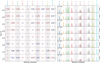 |
Fig. 9 Same as Fig. 7, but for the a0 parameter of the ζ(r) fitting function in Eq. (3). |
| In the text | |
|
Fig. C.1 Radial profiles for different quantities (gas temperature T, dust temperature Td, density n, and radial velocity υr) as density probability of our models’ sample (color plot), compared with Fig. 3 of Sipilä et al. (2022), at t = 7.19 × 10⁵ yr (dashed lines). The probability density is vertically normalized to have the same integral value (i.e., unity) at each radius. We note the log-scaled radius. |
| In the text | |
|
Fig. E.1 Density probability of the maximum error of predicting ζ(r) with NN. The mean, the median, and the 25 and 75 quartiles are respectively indicated as dashed, dotted, and solid lines. |
| In the text | |
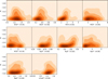 |
Fig. F.1 Same as Fig. 8, but for the a1 parameter of the ζ(r) fitting function in Eq. (3). |
| In the text | |
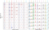 |
Fig. F.2 Same as Fig. 7, but for the abundance of C18O at 104 au ( |
| In the text | |
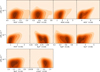 |
Fig. F.3 Same as Fig. 8, but for the abundance of C18O at 104 au ( |
| In the text | |
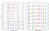 |
Fig. F.4 Same as Fig. 7, but for the collapse time factor τ. |
| In the text | |
Current usage metrics show cumulative count of Article Views (full-text article views including HTML views, PDF and ePub downloads, according to the available data) and Abstracts Views on Vision4Press platform.
Data correspond to usage on the plateform after 2015. The current usage metrics is available 48-96 hours after online publication and is updated daily on week days.
Initial download of the metrics may take a while.