| Issue |
A&A
Volume 702, October 2025
|
|
|---|---|---|
| Article Number | A2 | |
| Number of page(s) | 31 | |
| Section | Cosmology (including clusters of galaxies) | |
| DOI | https://doi.org/10.1051/0004-6361/202554520 | |
| Published online | 26 September 2025 | |
Dark matter halos modeled by polytropic spheres influenced by the relict cosmological constant and trapping polytropes forming supermassive black holes
Research Centre for Theoretical Physics and Astrophysics, Institute of Physics, Silesian University in Opava, Bezručovo nám. 13, 746 01 Opava, Czech Republic
⋆ Corresponding author: This email address is being protected from spambots. You need JavaScript enabled to view it.
Received:
13
March
2025
Accepted:
11
July
2025
Abstract
Aims. We study dark matter halos modeled by general relativistic polytropic spheres in spacetimes with the repulsive cosmological constant representing vacuum energy density, governed by a polytropic index, n, and a relativistic (cosmological) parameter, σ (λ), determining the ratio of central pressure (vacuum energy density) and central energy density of the fluid.
Methods. To give mapping of the polytrope parameters for matching the extension and mass of large dark matter halos, we study the properties of the polytropic spheres and introduce an effective potential of the geodesic motion in their internal spacetime. Circular geodesics enable us to find the limits of the trapping polytropes with central regions containing trapped null geodesics; supermassive black holes can be formed due to the instability of the central region against gravitational perturbations. The stability of the polytropic spheres relative to radial perturbations is determined. We match the extension and mass of the polytropes to the ones of dark matter halos related to large galaxies or galaxy clusters, with an extension of 100 < ℓ/kpc < 5000 and gravitational mass of 1012 < M/M⊙ < 5 × 10¹⁵. The velocity radial profiles of circular geodesics in the polytrope spacetimes are numerically compared to the observed velocity profiles.
Results. The observed velocity profiles simulated by the phenomenological dark matter halo density profiles can also be well matched by the velocity profiles of the exact polytrope spacetimes. The matching is made possible by the nonrelativistic polytropes for each value of n, with a relativistic parameter of σ ≤ 10−4 and a very low central energy density. Surprisingly, the matching works for “spread” relativistic polytropes with n > 3.3 and σ ≥ 0.1 when the central density can be much larger. The trapping polytropes forming supermassive black holes must have n > 3.8 and σ > 0.667. We thus explain the mass and structure of large galaxies and galaxy clusters, their extension limited by the cosmic repulsion, and the existence of black holes with mass M > 1010 M⊙ in very large galaxies; we suggest black holes with M ∼ 1012 M⊙ in large galaxy clusters.
Key words: stars: kinematics and dynamics / galaxies: halos / dark matter
© The Authors 2025
 Open Access article, published by EDP Sciences, under the terms of the Creative Commons Attribution License (https://creativecommons.org/licenses/by/4.0), which permits unrestricted use, distribution, and reproduction in any medium, provided the original work is properly cited.
This article is published in open access under the Subscribe to Open model. This email address is being protected from spambots. You need JavaScript enabled to view it. to support open access publication.
1. Introduction
The inflationary paradigm (Guth 1981; Linde 1990; Guth et al. 2014) and wide range of cosmological observations indicate the existence of dark energy demonstrating a repulsive gravitational effect. Specifically, it can be the vacuum energy, i.e., a very small relict repulsive cosmological constant, Λ > 0 (Krauss & Turner 1995; Ostriker & Steinhardt 1995; Krauss 1998; Bahcall et al. 1999; Armendariz-Picon et al. 2000; Wang et al. 2000; Carroll 2001). Observations of distant Ia-type supernova explosions indicate that starting at the cosmological redshift z ≈ 1 the expansion of the Universe is accelerated (Riess et al. 2004). In accordance with the inflationary paradigm, the total energy density of the Universe is very close to the critical energy density, ρcrit, corresponding to an almost flat Universe (Spergel et al. 2007; Tristram et al. 2024). The cosmological tests demonstrate that the dark energy represents about 70% of the energy content of the observable Universe (ρvac ∼ 0.7ρcrit) (Huterer & Shafer 2018). Then about 25% of the Universe energy content is in the form of dark matter, and the remaining 5% corresponds to the baryonic matter and the other forms of matter and fields (Brout et al. 2022). These results are confirmed by measurements of cosmic microwave background anisotropies by the space satellite observatory PLANCK (Planck Collaboration VI 2020). The dark energy equation of state is very close to those corresponding to the vacuum energy, i.e., to the repulsive cosmological constant. The value of the relict cosmological constant is estimated to be Λ ≈ 1.1 × 10−56 cm−2, and the vacuum mass density ρvac ∼ 10−29 g cm−3 (Planck Collaboration VI 2020).
The inflationary Universe stands at the base of the ΛCDM model that combines the role of dark energy represented by the relict cosmological constant, Λ, and cold dark matter (CDM), assumed to be relevant in the recent era of the Universe evolution Mukhopadhyay et al. (2008). The ΛCDM model can be considered as the standard cosmological model in the recent era of cosmological investigations, besides some difficulties with the interpretation of recent results (Blanchard et al. 2024). The exact form of the inflationary Universe remains an open problem, being under extensive debate, but the cosmic observations are introducing strong constraints on the considered inflationary models (Planck Collaboration X 2020).
In addition to cosmological models (Peebles & Ratra 2003), the cosmological and astrophysical consequences of the relict cosmological constant inferred from cosmological tests are explored within various spacetime frameworks. These include Einstein–Strauss vacuola models (Stuchlík 1983, 1984; Uzan et al. 2011; Grenon & Lake 2010; Fleury et al. 2013; Arraut 2014b; Faraoni et al. 2015; Faraoni 2016), and the McVittie model (McVittie 1933), which describes local mass concentrations embedded in an expanding Universe (Nolan 1998, 1999; Nandra et al. 2012; Kaloper et al. 2010; Lake & Abdelqader 2011; da Silva et al. 2013; Nolan 2014).
The very important role of the repulsive cosmological constant has also been demonstrated for astrophysical processes (accretion disks, jets) related to active galactic nuclei (Stuchlík et al. 2018, 2020) and their central supermassive black holes (Stuchlík & Calvani 1991; Lake 2002; Stuchlík & Hledík 2002; Stuchlík & Slaný 2004; Kraniotis 2004; Kraniotis et al. 2005; Kraniotis 2007; Cruz et al. 2005; Stuchlík et al. 2000; Slaný & Stuchlík 2005; Stuchlík 2005; Sereno 2008; Müller 2008; Schücker & Zaimen 2008; Villanueva et al. 2012; Rezzolla et al. 2003; Kagramanova et al. 2006; Aliev 2007; Chen & Wang 2008; Iorio 2009; Hackmann et al. 2010; Kološ & Stuchlík 2010; Hendi & Momeni 2011; Hendi et al. 2012; Gu & Cheng 2007; Wang & Cheng 2012; Stuchlík et al. 2009; Pugliese & Stuchlík 2016, 2024). On the other hand, the Kerr superspinars representing an alternative to the supermassive black holes in active galactic nuclei, based on the String theory (Gimon & Hořava 2004; Boyda et al. 2003; Gimon & Hořava 2009; Stuchlík & Schee 2012) and exhibiting a variety of unusual physical phenomena (de Felice 1974, 1978; Stuchlík 1980; Hioki & Maeda 2009; Stuchlík & Schee 2013), could also be relevant (Stuchlík et al. 2011). The pseudo-Newtonian potential related to the spherically symmetric spacetimes with the repulsive cosmological constant (Stuchlík & Kovář 2008) serves well in studies of the motion of interacting galaxies (Stuchlík & Schee 2011).
The general relativistic polytropic spheres in spacetimes with a repulsive cosmological constant were analyzed in detail by Stuchlík et al. (2016). That work generalizes the case of spheres with uniform energy density but radius-dependent pressure, which formally correspond to polytropes with index n = 0. These configurations are often used as a test bed for studying the properties of relativistic polytropes, as their structure equations can be solved analytically using elementary functions (Stuchlík 2000; Böhmer 2004; Nilsson & Uggla 2000b; Böhmer & Fodor 2008). Two important results were obtained: first, the polytropic spheres cannot exceed the static radius where their gravitational attraction is just balanced by cosmic repulsion (Stuchlík 1983; Stuchlík & Hledík 1999), giving a natural limit on gravitationally bound systems in the accelerated Universe; second, the extension and mass of the polytropic spheres can be comparable even to the extension and mass of dark matter halos of large galaxies and galaxy clusters (Stuchlík et al. 2016).
The general relativistic polytropic spheres enable a very useful, physically relevant idealization of fluid configurations under various conditions, giving a simple and coherent picture of all the potentially relevant relativistic phenomena influencing matter configurations across different distance scales. The application of the polytropic equations of state for modeling of neutron (or quark) stars is well known. In the basic approximation, the degenerate Fermi gas can be represented by the equation of state with polytropic index n = 3/2 in the nonrelativistic limit, and n = 3 in the ultrarelativistic limit (Shapiro & Teukolsky 1983). Polytropic state equations with various values of the polytropic index, n, are used to give a precise approximation of relativistic equations of state governing the interior of neutron stars (Özel & Psaltis 2009; Lattimer & Prakash 2001); one can even use several polytropic state equations to cover the neutron star core (Alvarez-Castillo et al. 2017).
On the other hand, extremely extended general relativistic polytropic spheres can serve as models of halos of dark matter (DM) in galaxies or even galaxy clusters; the preliminary results (Stuchlík et al. 2016; Arbañil & Moraes 2020) demonstrate that nonrelativistic polytropes can represent halos made of CDM, while the relativistic polytropes can represent halos made of warm dark matter (WDM), or could be applied in more complex situations, mixing the cold and warm DM, or other influences (such as those of standard baryonic matter). Very interesting are galaxies existing in the early stages of expansion of the Universe, observed at the cosmological redshift z > 6. Of particular interest are the active nuclei of galaxies containing supermassive black holes that in some cases have masses exceeding 1010 M⊙ (Ziolkowski 2005), as the standard explanation of the successive growth of black holes that initially have a mass of the stellar order M ≤ 100 M⊙ requires specially ordered conditions during growth on small timescales to such extreme values of the black hole mass.
Despite enormous efforts in both theoretical and experimental particle physics, the composition of DM remains unknown; a large variety of possible (but controversial) candidates of both cold and warm DM can be considered acceptable. Due to the lack of a clear DM candidate coming from particle physics, we are free to choose any parameters of the polytrope equation of state to test observationally relevant predictions of the general relativistic polytropic spheres related to their extension, mass and the corresponding velocity curves. Here, in matching the extension and mass of halos related to large galaxies and galaxy clusters, we test the simple relativistic or nonrelativistic polytropic spheres represented by a single ensemble of the polytrope parameters. However, in modeling realistic large galaxies and galaxy clusters, different polytropic indexes, n, have to represent different dynamics of the halo rather than being a direct signature of a concrete form of dark matter. Moreover, we can expect polytropes combined in “series,” or in a “parallel” way as a mixture of two or more types of fluid (representing various forms of matter in halos, for example, dark matter combined with ordinary matter).
Cold dark matter halos are now widely regarded as the most natural explanation for the hidden mass in galaxies, providing a consistent framework for describing the dynamics of their outer regions (Bosma 1981; Rubin et al. 1982). These foundational studies have been extensively reviewed and synthesized by Salucci (2019), who offers an up-to-date overview of dark matter distributions across different galactic systems. Additional evidence of the gravitational potential wells binding galaxy clusters has been provided by analyses of gravitational lensing and large-scale structure (Barreira et al. 2015; Sartoris et al. 2014).
The CDM halos are usually treated in the Newtonian approximation (Binney & Tremaine 1988; Iorio 2010; Navarro et al. 1997; Stuchlík & Schee 2011; Cremaschini & Stuchlík 2013) or in the pseudo-Newtonian approximation (Stuchlík & Schee 2011). We consider here as the halo model the fully general relativistic spherically symmetric static configurations of perfect fluid with a polytropic equation of state (Tooper 1964) and modify them by introducing the vacuum energy represented by the repulsive cosmological constant restricted by the recent cosmological observations. Details of the physical processes inside the polytropic spheres are not considered; the power law relating the total pressure to the total energy density of matter is assumed. The polytropic approximation seems to be applicable in the dark matter models assuming weakly interacting particles (see, for example, Börner (1993), Kolb & Turner (1990), Cremaschini & Stuchlík (2013)), and also for strongly interacting particles as is shown in Böhmer & Harko (2007).
Describing CDM halos by using polytropic spheres treated in the nonrelativistic regime has a long history and has been realized in various approaches. The models are considered in the framework of both Newtonian physics (see Saxton & Ferreras 2010) or in a linearized Einstein general relativity approach (see Arbey et al. 2003). A special approach to model DM halos is represented by the Bose-Einstein condensates (based on scalar fields, and sometimes called Einstein-Klein-Gordon stars) that were treated in both Newtonian (Guzmán & Ureña-López 2006; Luu et al. 2020; Emami et al. 2020) and general relativistic approaches (Sahni & Wang 2000; Matos et al. 2009; Alcubierre et al. 2018). The Bose-Einstein condensates are governed by the Gross-Pitaevskii equation, representing a special form of the Schrödinger-Poisson equation – this approach was developed in both a Newtonian and a fully general relativistic form in Böhmer & Harko (2007), with both of them leading to a special form of the polytropic equation of state. We have to stress that the results of these works related to the fitting of the models to observed galaxies indicate different dark matter parameters, connected to the polytropes, while applied to different galaxies. These results thus indicate that the polytropic spheres have to be considered as structural models reflecting different dynamics of halos that should be constituted in a complex way, being dependent also on the total mass, and probably also on their history. In this sense we have to consider also the possibility of describing a galaxy, or a galaxy cluster, with two polytropes (that have different parameters) whereby one of them is related to the central part of the galaxy, while the other is related to the external part. We can thus combine the polytropes in a “series” way, but also in a “parallel” way, while considering two-component spheres in a common space – this can be an inverse to the situations in which neutron stars are studied as being occupied additionally by dark matter (Narain et al. 2006; Hall et al. 2010; Kouvaris 2012).
Quite recently, a two-component bosonic dark matter model was introduced in Castelo Mourelle et al. (2025) that enables the treatment of dark matter subhalos. Very interesting is another recent study of the formation and evolution of scalar field dark matter cosmologies representing an alternative to CDM halos Foidl et al. (2023).
The role of the dark energy represented by the repulsive cosmological constant in the polytropic structures was started for the simplest n = 0 polytropes in Stuchlík (2000), Böhmer (2004). The fluid spheres under the influence of the cosmological constant were also treated in (Böhmer & Fodor 2008; Stuchlík et al. 2016; Gabbanelli et al. 2019; Arbañil & Moraes 2020). Here we concentrate attention on polytropic spheres treated in both nonrelativistic and relativistic regimes under the influence of the relict cosmological constant.
The rough estimates realized in Stuchlík et al. (2016) indicate that the nonrelativistic polytropic spheres could represent the CDM halos. However, there is a strong indication of the failure of the CDM halo model at small scales in recent galaxies (Gariazzo et al. 2017; Murgia et al. 2017). On the other hand, the applicability of the WDM model (Bode et al. 2009; Baur et al. 2016), especially in the case of primeval galaxies, is seriously considered (Lapi & Danese 2015). There are a variety of possible non-CDM halo candidates, starting at the standard possibilities of WDM represented by sterile neutrinos (Adhikari et al. 2017) or axions (Marsh & Silk 2013; Hui et al. 2017). Anderhalden et al. offer mixed C&WDM matter (Anderhalden et al. 2012); also, self-interacting DM is seriously taken into account (Raccanelli et al. 2016).
For the description of most of the non-cold DM halo models, the relativistic polytropic spheres have to be relevant, and they thus deserve attention in our study. Therefore, we present here a detailed mapping on the possibility of matching the extension and mass of dark matter halos of large galaxies or galaxy clusters by extremely extended polytropic spheres that could occur for sufficiently large polytropic indexes, 3.3 < n < 5, when such polytropes can exist, if the relativistic parameter is close to the critical values, σcrit(n) (Nilsson & Uggla 2000b; Stuchlík et al. 2016). Recall that for σ = σcrit(n) and vanishing vacuum energy, the polytropic spheres have unlimited extension, but the relict cosmological constant introduces a relevant restriction on their extension, which will be demonstrated in the present paper for selected representative values of the polytropic index, n.
Moreover, we demonstrate a very interesting property of highly relativistic polytropes that contain a region of trapped null geodesics (Novotný et al. 2017). We show that in the trapping zone an efficient gravitational instability causes gravitational collapse of the matter and conversion of the zone of trapping to a central black hole containing nearly 10−3 of the halo mass (Stuchlík et al. 2017). If the polytropic parameters are properly tuned, the trapping polytrope can be extremely extended, representing a dark matter halo of a large galaxy or a galaxy cluster and having a mass of Mhalo-galaxy > 1012 M⊙, and the central supermassive black hole created in the trapping zone can have a mass of MBH > 109 M⊙ (Stuchlík et al. 2017). The black hole mass can even exceed M ∼ 1012 M⊙ if centered in a large galaxy cluster with Mhalo-cluster > 1015 M⊙. The gravitational instability of the central “trapping” region of extremely extended trapping polytropes can thus serve as an alternative model of the formation of supermassive black holes in the high-redshift (z > 6) large galaxies or their clusters. As the original study concerning the gravitational instability of extended trapping polytropes was conducted under simplified assumptions about a vanishing cosmological constant, while its influence on the extension of such polytropic spheres can be crucial, we devote special attention in the present paper to the study of the role of the cosmological constant in constraining the mass and extension of the extremely extended trapping polytropes1.
We show that the polytropic spheres considered in the nonrelativistic regime can be satisfactorily applied to describe and qualify the dwarf galaxies demonstrating the so-called cusp-core problem (Novotný et al. 2021). In the present paper, we extend our previous works on general relativistic polytropes (Stuchlík et al. 2016) and the trapping polytropes (Novotný et al. 2017; Stuchlík et al. 2017) to a detailed study of the role of dark energy and the polytropes related to WDM.
In the first part of our work (Sections II–VI), we give the polytrope study for the general situation with the role of the dark energy governed by the dimensionless “vacuum” parameter, λ = ρvac/ρc, relating the vacuum (or false vacuum) mass density, ρvac, and the central density, ρc of the polytropic fluid. We extend our previous studies (Stuchlík et al. 2016; Novotný et al. 2017) for the polytropic parameter going up to n = 4.5, summarizing and extending the previous results in Sections II-IV. In Section 5 we newly introduce the discussion of geodesic motion of test particles in the polytropic structures, as the circular geodesics are expected to represent the orbital motion of the galactic matter that should correspond to the observed rotation curves, and discuss in detail the influence of the parameter λ on the trapping polytropes. In Section VI we also include a detailed study of the dynamic stability of the polytropic spheres with the polytropic parameter going up to n = 4.5 and give the restrictions corresponding to some selected values of the vacuum parameter, λ, on polytrope dynamic stability, including the case of trapping polytropes. We demonstrate that all the trapping polytropes are dynamically unstable. For selected values of λ, we present a detailed mapping of the ratio of a polytrope extension and static radius corresponding to the polytrope; this gives a detailed illustration of how the cosmological constant influences the polytrope properties. The general results obtained for a free parameter, λ, can be applied directly in the case of the observed repulsive dark (vacuum) energy, ρvac = 10−29 g cm−3; in this case the general limits related to the parameter λ are transformed on the limits related to the polytrope central density, ρc. Another possibility could be to obtain some estimates for polytropes influenced by a false vacuum energy density related to various phase transitions in the early Universe – in a way similar to those connected to accretion structures related to the Schwarzschild-de Sitter black hole spacetimes (Stuchlík et al. 2000).
In the second part (Sections VII-XI) we focus on the mapping of possible matching of the polytropes to large galaxies and galaxy clusters. In this case we fully concentrate on the role of the observed relict cosmological constant, Λ ≈ 1.1 × 10−56 cm−2, and the related vacuum mass density, ρvac ∼ 10−29 g cm−3 (Planck Collaboration VI 2020). In such a case, fixing the vacuum parameter, λ, fixes the central mass density of the polytrope. We realize a detailed mapping of the parameters of polytropic spheres representing large dark matter halos that have an extension and mass corresponding to the ones of large galaxies and galaxy clusters; the trapping polytropes enabling the creation of supermassive black holes in their central region (Stuchlík et al. 2017) are included. We present a detailed study of the possibility of matching the extension and mass of DM halos separately for the nonrelativistic and relativistic polytropic spheres. For selected typical polytropic halos, we give the density and metric coefficient radial profiles. We also apply the circular geodesics derived for the interior of the polytropic spheres as possible fits to the rotational curves observed in large galaxies and galaxy clusters by comparing the velocity radial profiles of the polytrope circular geodesics to the velocity radial profiles corresponding to the standard Navarro-Frenk-White or Burkert models of DM halos. A more detailed study of the velocity radial profiles, combining the polytropic regions representing the outer regions of large galaxies with the galaxy bulge and galaxy disk regions dominating the inner regions of large galaxies, or models of combined polytropes applied to individual galaxies or galaxy clusters, is planned for a future paper.
2. Polytropic spheres with cosmological constant
The line element of a spherically symmetric, static spacetime, expressed in terms of the standard Schwarzschild coordinates, reads
 (1)
(1)
The metric contains just two unknown functions of the radial coordinate, Φ(r) and Ψ(r). Matter of the static configuration is assumed to be a perfect fluid with the stress-energy tensor
 (2)
(2)
where Uμ denotes the four-velocity of the fluid. In the rest frame of the fluid, ρ = ρ(r) represents the mass-energy density and p = p(r) represents the isotropic pressure.
We restrict our attention to the simplest direct relation between the mass-energy density and pressure given by the polytropic equation of state,
 (3)
(3)
where n denotes the ‘polytropic index’ assumed to be a given constant. K is a constant determined by the thermal characteristics of a given fluid spherical configuration by specifying the density, ρc, and pressure, pc, at the center of the polytropic sphere. It is determined by the total mass and radius of the configuration, and the so-called relativistic parameter (Tooper 1964),
 (4)
(4)
For a given pressure, the density is a function of temperature, and thus the constant, K, contains the temperature implicitly.
Note that the polytropic equation represents a limiting form of the parametric equations of state for a completely degenerate gas at zero temperature, which is relevant, for example, for neutron stars. Then both n and K are universal physical constants (Tooper 1964). In fact, the simple polytropic law assumption enables us to obtain basic properties of the fluid configurations governed by the relativistic laws. For example, the equation of state of the ultrarelativistic degenerate Fermi gas is determined by the polytropic equation with the adiabatic index Γ = 4/3 corresponding to the polytropic index n = 3, while the nonrelativistic degenerate Fermi gas is determined by the polytropic equation of state with Γ = 5/3, and n = 3/2 (Shapiro & Teukolsky 1983).
The structure of the general relativistic polytropic spheres is determined by the Einstein field equations,
 (5)
(5)
containing the dark vacuum energy that is represented by the cosmological constant term, and by the local energy-momentum conservation law,
 (6)
(6)
2.1. Structure equations
For the structure of the polytropic spheres, only the (t)(t) and (r)(r) components of the Einstein field equations are relevant (the (θ)(θ) and (ϕ)(ϕ) components give dependent equations) (Tooper 1965). The structure is governed by the two structure functions. The first one, θ(r), is related to the mass-energy density radial profile, ρ(r), and the central density ρc (Tooper 1964)
 (7)
(7)
with the boundary condition θ(r = 0) = 1. The second one is the mass function of the polytropic configuration given by the relation
 (8)
(8)
with the integration constant chosen to be m(0) = 0, to guarantee the smooth spacetime geometry at the origin (see Ref. Misner et al. 1973). At the edge of the configuration at r = R, there is ρ(R) = p(R) = 0, and the total mass of the polytropic configuration M = m(R). Outside the polytropic configuration, the spacetime is described by the vacuum Schwarzschild-de Sitter metric.
Projection of  orthogonal to Uμ implies the equation of hydrostatic equilibrium describing the balance between the gravitational force and pressure gradient that can be put into the Tolman–Oppenheimer–Volkoff (TOV) form modified by the presence of a nonzero cosmological constant (Stuchlík 2000):
![Mathematical equation: $$ \begin{aligned} \frac{\mathrm{d} p}{\mathrm{d} r} = - (\rho c^{2} + p) \frac{G m(r)/c^{2} - \Lambda r^{3}/3 + 4\pi G p r^{3}/{c^4}}{r \left[r-2G m(r)/c^{2} - \Lambda r^{3}/3 \right]}\, . \end{aligned} $$](/articles/aa/full_html/2025/10/aa54520-25/aa54520-25-eq10.gif) (9)
(9)
Then the structure equations of the polytropic spheres related to the two structure functions, θ(r) and m(r), and the three parameters, n, σ, and Λ, can be put into the form (Stuchlík et al. 2016)
 (10)
(10)
We introduce the length factor, ℒ, which defines the characteristic length scale of the polytropic sphere,
![Mathematical equation: $$ \begin{aligned} \mathcal{L} = \left[\frac{(n + 1)K\rho _{\rm c}^{1/n}}{4\pi G\rho _{\rm c}}\right]^{1/2} = \left[\frac{\sigma (n + 1)c^{2}}{4\pi G\rho _{\rm c}}\right]^{1/2}\,. \end{aligned} $$](/articles/aa/full_html/2025/10/aa54520-25/aa54520-25-eq12.gif) (11)
(11)
Similarly, we define the mass factor, ℳ, which gives the characteristic mass scale of the polytropic sphere,
 (12)
(12)
Using these factors, we transform the structure Equations (10) and (11) into a dimensionless form by introducing the dimensionless radial coordinate,
 (13)
(13)
and defining the dimensionless quantities
 (14)
(14)
 (15)
(15)
Here, ν(ξ) represents the dimensionless mass function, and λ denotes the dimensionless cosmological constant, both associated with the polytropic sphere. The vacuum energy density, ρvacc2, and the cosmological constant, Λ, are related by
 (16)
(16)
The dimensionless structure equations (10) and (11) take the form
 (17)
(17)
 (18)
(18)
For fixed parameters n, σ, λ, equations (18) and (19) have to be solved simultaneously under the boundary conditions
 (19)
(19)
It follows from (19) and (20) that ν(ξ)∼ξ3 for ξ → 0 and, according to Eq. (18), there is
 (20)
(20)
The boundary of the polytropic sphere, r = R, is represented by the first zero point of θ(ξ), denoted as ξ1:
 (21)
(21)
The solution ξ1 determines the surface radius of the polytropic sphere, and the solution ν(ξ1) determines its gravitational mass. In Fig. 1 we illustrate possible types of the behavior of the function θ(ξ), including the limiting case governed by the value of the cosmological parameter.
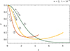 |
Fig. 1. Dependence of the pressure, θ, to the dimensionless radial coordinate, ξ. The surface of the polytropic sphere is determined by the first zero of θ(ξ), if it exists. Such points are depicted on the plot by solid dots, see curves ① and ②. The expected θ-curve (corresponding to pressure) is a monotonically decreasing function. As a manifestation of the influence of the cosmological parameter λ, the θ function can start to increase even before the first zero is reached, see curve ③. Change of monotonicity occurs in local minimum dθ/dξ = 0 and if such a minimum occurs at ξ1, where θ(ξ1) = 0, such a point is identified as the “static radius of the external spacetime” of such a polytrope, ξs = 3ν(ξ1)/2λ, see curve ②. If θ(ξmin) > 0 at such a minimum localized at ξmin, like on the curve ③, the ratio |
The radius of the polytropic sphere reads
 (22)
(22)
while the mass of the sphere is given by
 (23)
(23)
2.2. Characteristics of the polytropic spheres
The general relativistic polytropic spheres are determined by the functions θ(ξ) and ν(ξ) of the dimensionless coordinate ξ and by the length and mass scales, ℒ, ℳ.
The energy density, pressure, and mass-distribution radial profiles are given by the relations
 (24)
(24)
 (25)
(25)
 (26)
(26)
The temporal metric coefficient of the internal spacetime of the polytrope can be expressed in the form
![Mathematical equation: $$ \begin{aligned} e^{2\Phi } = (1 + \sigma \theta )^{-2(n + 1)}\left\{ 1-2\sigma (n + 1) \left[\frac{\nu (\xi _{1})}{\xi _{1}} + \frac{1}{3}\lambda \xi _{1}^{2}\right] \right\} \, , \end{aligned} $$](/articles/aa/full_html/2025/10/aa54520-25/aa54520-25-eq30.gif) (27)
(27)
while the radial metric coefficient of the internal spacetime reads
![Mathematical equation: $$ \begin{aligned} e^{-2\Psi } = 1 - 2\sigma (n + 1)\left[\frac{\nu (\xi )}{\xi } + \frac{1}{3}\lambda \xi ^{2}\right]\, . \end{aligned} $$](/articles/aa/full_html/2025/10/aa54520-25/aa54520-25-eq31.gif) (28)
(28)
In the exterior of the polytropic sphere, at ξ > ξ1, the metric coefficients take the form
![Mathematical equation: $$ \begin{aligned} e^{2\Phi } = e^{-2\Psi } = 1 - 2\sigma (n + 1)\left[\frac{\nu (\xi _1)}{\xi } + \frac{1}{3}\lambda \xi ^{2}\right]\, . \end{aligned} $$](/articles/aa/full_html/2025/10/aa54520-25/aa54520-25-eq32.gif) (29)
(29)
The compactness, determining the effectiveness of the gravitational binding of the polytropic sphere, is given by the relation
 (30)
(30)
where we have introduced the standard gravitational radius of the polytropic sphere that reflects its gravitational mass in length units, rg = 2GM/c2. The compactness, 𝒞, of the polytropic sphere can be represented by the gravitational redshift of radiation emitted from the surface of the polytropic sphere (Hladík & Stuchlík 2011). It is clear that the polytropic spheres representing the DM halos must be of extremely low compactness, as the gravitational radius has to be located deep in the central region of such spheres.
The expressions for the gravitational energy and binding energy of the polytropic spheres can be found in Stuchlík et al. (2016), where the analytical expression in terms of elementary functions is also given for the special class of uniform energy density spheres, that is, polytropes with index n = 02. Notice that for vanishing cosmological constant, the polytrope structure equations are fully determined only by the parameters n and σ, but the extension and mass scales are governed also by the central energy density ρc. The cosmological constant breaks this degeneracy of the structure equations, as the central energy density enters them due to its mixing with the vacuum energy density in the parameter λ.
3. External spacetime and length scales
The external vacuum Schwarzschild–de Sitter spacetime is represented by the same gravitational mass parameter, M, and the same cosmological constant, Λ, as those characterizing the internal spacetime of the polytropic sphere and is given by the metric coefficients
 (31)
(31)
There are two event horizons related to the external vacuum spacetime – the inner black hole horizon, and the outer cosmological horizon (Stuchlík 1983; Stuchlík & Hledík 1999; Stuchlík et al. 2000). In astrophysically plausible situations, even for the most massive black holes in the central part of giant galaxies, for example in the quasar TON 618 with the mass M ∼ 6.6 × 10¹⁰ M⊙ (Ziolkowski 2008), or for masses related to the whole giant galaxies containing an extended DM halo, and for clusters of galaxies having mass up to M ∼ 1015 M⊙, the related black hole horizon radius (hidden deeply inside the galaxy or the cluster) and the cosmological horizon radius are given with very high precision by the simple formulae (Stuchlík et al. 2009)
 (32)
(32)
The event horizons thus give two characteristic length scales of the SdS spacetimes. Of course, the black hole horizon is located inside the polytropic spheres, and thus physically irrelevant, while the cosmological horizon is located outside the polytropic sphere, at an extremely large distance from the polytropic sphere for the observationally given value of the relict cosmological constant Λ ∼ 10−56 cm−2. These two characteristic length scales can be combined to give a dimensionless parameter characterizing the Schwarzschild–de Sitter geometry (Stuchlík & Hledík 1999)
 (33)
(33)
For the observationally estimated repulsive cosmological constant Λ ∼ 1.1 × 10−56 cm−2, the cosmological parameter y takes extremely small values, if we consider the stellar mass black holes and galactic center black holes; very small values are obtained even for the largest compact objects of the Universe, i.e., the extremal central supermassive black holes in the active galactic nuclei and the giant galaxies or their clusters (Stuchlík et al. 2000; Stuchlík 2005).
A third length scale characterizing the SdS vacuum spacetimes determines the boundary of the gravitationally bound system behind which the cosmic repulsive effects start to be effective. The third scale is given by the so-called static radius (sometimes also called the turn-around radius) (Stuchlík & Hledík 1999; Stuchlík & Slaný 2004; Stuchlík 2005; Grenon & Lake 2010; Stuchlík & Schee 2011; Arraut 2015, 2013, 2014a; Faraoni et al. 2014, 2015) defined by
 (34)
(34)
where the gravitational attraction of the central mass source is just balanced by the cosmic repulsion. All test particle (or fluid) bound orbits, such as the circular orbits, have to be located inside the static radius sphere (Stuchlík & Slaný 2004; Stuchlík et al. 2009).
A detailed discussion of the properties of the general relativistic polytropic spheres in spacetimes with the repulsive cosmological constant has been presented for properly selected values of the polytropic parameter n in Stuchlík et al. (2016), where the special case of uniform density spheres corresponding to the polytropes with n = 0 is also included. It has been explicitly demonstrated that the role of the cosmological constant could be very strong for largely extended polytropic spheres.
It is instructive to relate the three characteristic length scales of the external vacuum spacetime to the polytrope length scale ℒ, the sphere radius R = ℒξ1 and its central density. For spheres with a very large central density, related to the central densities of very compact objects such as neutron stars or quark stars, the length scale is comparable to the black hole horizon scale (gravitational radius), with decreasing central density the polytrope length scale increases. On the other hand, for the observationally estimated cosmological constant Λ ∼ 1.1 × 10−56 cm−2, the length scale and extension of all astrophysically relevant polytropic spheres are much lower than the length scale of the cosmological horizon.
For the polytropic spheres with extremely low central energy density that are also extremely extended for sufficiently low relativistic parameter (σ ≤ 10−4, i.e., in the nonrelativistic regime), the crucial role is played by the length scale of the static radius since it represents the uppermost limit on the extension of the general relativistic polytropic spheres with the cosmological constant (Stuchlík et al. 2016). Note that in the case of the relativistic polytropic spheres with large polytropic index (n > 3.3), the extremely extended polytropic spheres could also exist for much larger values of the central energy density, and large values of the relativistic parameter (σ > 0.1), being very close to the critical values implying the special character of the density and pressure profiles – their extension is also restricted by the static radius (Stuchlík et al. 2016). Here we discuss in detail the possibility that such extremely extended polytropic spheres could represent the DM halos, with the extension and mass of the halos given by the standard observation estimates. The CDM halos can be represented by nonrelativistic polytropes with σ ≪ 1. On the other hand, the warm DM halos can be represented by relativistic polytropes with σ > 0.1, if its value is close to the critical value predicting unlimited polytropic spheres for vanishing cosmological constant (Nilsson & Uggla 2000b; Stuchlík et al. 2016). Note that the trapping polytropes can be both compact and extremely extended, depending on the polytropic index, n.
We first summarize the limits on the existence of the polytropic spheres related to the dimensionless cosmological parameter λ that can be directly related to the observationally restricted cosmological constant, the extension and mass of the polytropes as influenced by the parameter λ, and the circular geodesics of the internal polytrope spacetimes that can mimic the rotational curves observed in galaxies. Special attention is devoted to the trapping polytropes governed by the behavior of the null circular geodesics.
4. Constraints on general relativistic polytropes with cosmological constant
We briefly discuss the construction of the models of the general relativistic polytropes with n > 0 and demonstrate the dependence of their existence on the cosmological parameter λ; details can be found in Stuchlík et al. (2016). By integrating numerically the two differential structure equations for a fixed polytropic index n > 0, we obtain a sequence of polytropic spheres determined by the relativistic parameter σ, and the cosmological parameter λ that is considered as a free parameter. If the cosmological constant and vacuum mass density are fixed, the polytrope central density, ρc, can be considered as a free parameter governing along with the vacuum density the dimensionless parameter, λ. Up to Section 6, we keep λ as a free parameter making some comments related to the special value of relict vacuum mass density ρvac ∼ 10−29 g cm−3.
The lowest solution, ξ1, of the equation θ(ξ) = 0 (if it exists, see Fig. 1) determines the dimensional radius of the polytropic sphere R = ℒξ1. The dimensionless mass parameter, ν(ξ1), determines the polytrope gravitational mass, M = ℳν(ξ1). The radial profiles of the mass-energy density, pressure, gravitational mass parameter, and the metric coefficients of the polytropic sphere are determined by the functions ρ(ξ; n, σ, λ), p(ξ; n, σ, λ), ν(ξ; n, σ, λ), gtt(ξ; n, σ, λ), grr(ξ; n, σ, λ) and are described in detail, along with other characteristics such as the gravitational and binding energy, in Stuchlík et al. (2016); characteristics can be found in Zenodo. Here we concentrate our attention on the extension R and mass M of the polytropic spheres and limits on the allowed values of R and M. These characteristics of the polytrope spheres can be directly related to the extension and mass of galaxies and galaxy clusters.
4.1. Limits on the general relativistic polytropes
The role of the cosmological parameter λ is concentrated in putting strong limits on the existence of polytropic spheres in dependence on both the polytropic index n and the relativistic parameter σ. The critical values of the cosmological parameter given by the function λcrit = λcrit(n, σ) limit the existence of polytropic spheres; they are determined by numerical calculations and are illustrated as functions of the relativistic parameter σ for selected representative values of n in Figs. 2a and b. For fixed values of n and σ, the critical parameter λcrit(n, σ) determines the minimal value of the central energy density,
 (35)
(35)
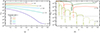 |
Fig. 2. Dependence of critical value, λcrit, on relativistic parameter, σ. On the left we demonstrate the behavior for the polytropic index n < 3 and on the right for n > 3. The gray line on the right highlights the restriction λ = 10−46 g cm−3. The configurations for particular polytropic index n can only exist below the corresponding curve λcrit(n; σ). |
allowing for the existence of static polytropic spheres, if the vacuum mass density is assumed to be known. (Assuming the observationally estimated Λ ∼ 10−56 cm−2 we can obtain limits on polytropes in the recent state of the Universe.)
For σ < σc(min)(n, σ) static polytropes cannot exist due to the cosmic repulsion. At σ = σc(min), the configuration reaches a limiting case in which the surface is located at the static radius. The situation is similar to the case of the accretion structures orbiting a Schwarzschild-de Sitter black hole that also must be restricted to the region located under the static radius given by the black hole mass M and the relict cosmological constant Λ (Stuchlík et al. 2000; Boonserm et al. 2020); note that the static radius in the Kerr-de Sitter black hole spacetimes is determined in identical form as those related to the Schwarzschild-de Sitter spacetimes, being independent of the black hole rotational parameter (Stuchlík & Slaný 2004). The static radius thus plays a crucial role for the gravitationally bound systems treated in the stationary situations. However, it also has a crucial role in the fully dynamic situations related to the models of black holes in the expanding Universe (Faraoni et al. 2015; Faraoni 2016; Bhattacharya et al. 2017; Lapierre-Léonard et al. 2017; Perlick et al. 2018; Nojiri et al. 2018; Boonserm et al. 2020) – in these models the so-called “turn-around” radius is introduced that separates the gravitationally bound and expanding regions, being determined by an identical form as the static radius of the Schwarzschild-de Sitter black hole spacetimes. It has also been demonstrated that the cosmic repulsion of the vacuum energy can significantly influence the motion of small satellite galaxies in the field of a large galaxy, even if considered just above its static radius (Stuchlík & Schee 2011).
However, the effects of vacuum energy (relict cosmological constant) can be clearly demonstrated only in the far future, during the strongly vacuum energy dominated epoch. In the present state of the Universe expansion, the evolution of the DM halos should be governed by a wide range of other influences, such as mass infall, interactions of halos, and their mergers (Foidl et al. 2023) that would be masking the role of the vacuum energy. From the point of view of the dynamics of the dark matter halos, recent work on the formation and evolution of CDM and scalar field dark matter models (Foidl et al. 2023) brings interesting results demonstrating possible expansion of halos after mass infall vanishing, due to the background pressure decrease caused by the Universe expansion.
The polytropic spheres are allowed at regions of the parameter space located below the critical curves. The character of the critical function λcrit(n, σ) strongly depends on the value of the polytropic index n. Generally, it increases with n decreasing. The critical function λcrit(σ; n) demonstrates two characteristic regimes of its behavior in dependence on the polytropic index n. Since it is known that for n > 3.3, the critical points of the relativistic parameter exist, denoted as σf(n), when no limit on extension of the polytropic sphere exists, and for n ≥ 5 no static polytropic spheres can exist for any values of σ (Nilsson & Uggla 2000a), we construct examples of the critical function λcrit(σ; n) in the first regime, for n ≤ 3, in Fig. 2a, and examples of the λcrit(σ; n) function in the second regime, for 3.4 < n < 5, in Fig. 2b. In Fig. 2a we cover the standard values of the polytropic index, for the nonrelativistic fluid with n = 3/2, and n = 3 for the ultrarelativistic fluid; we add the critical functions for some values n < 3/2, namely n = 0.5, 1, and for n = 2, 2.5. In Fig. 2b we give construction of the critical function λcrit(σ; n) for the values of the polytropic index n implying the existence of the critical values of the relativistic parameter, σf(n), when the limits on the existence of polytropic spheres vanish for vanishing cosmological parameter λ; the values of n = 3.5, 4, 4.5 are chosen. Extension of the critical curves is in all the considered cases restricted by the value of the relativistic parameter σ corresponding to the equality of the velocity of sound and the velocity of light (the so-called causality limit) – for details, see Stuchlík et al. (2016).
In the first regime (Fig. 2a), for n ≤ 3, the function λcrit(σ; n) slightly monotonically decreases with σ increasing; it is limited by the value of λcrit = 10−7 even in the limit of σ → 1. In the special case of n = 3, it decreases from the starting point λcrit(σ = 0; n = 3) = 3 × 10⁻³ down to λcrit(σ = 0.7; n = 3) = 10−7 and remains constant with increasing values of σ.
In the second regime (Fig. 2b), for n > 3.3, the function λcrit(n; σ) loses its monotonic character, and there are forbidden polytropes for some special values of the relativistic parameter σ in dependence on the polytrope index, as they should have infinite extension. For n = 3.5, the polytropic spheres are forbidden for one specific value of σ1 (n = 3.5) = 0.3131. For n = 4, there are two specific forbidden values of σ1 (n = 4) = 0.1501, σ2 (n = 4) = 0.3364. A third forbidden configuration with n = 4 corresponds to σ breaking the causality limit at σ3 (n = 4) = 0.8341, and is not considered here. For n = 4.5, there exists an ensemble of 8 critical values of the relativistic parameter, namely: σ1 (n = 4.5) = 0.0593, σ2 (n = 4.5) = 0.1131, σ3 (n = 4.5) = 0.1771, σ4 (n = 4.5) = 0.2696, σ5 (n = 4.5) = 0.399, σ6 (n = 4.5) = 0.5292, σ7 (n = 4.5) = 0.6510, σ8 (n = 4.5) = 0.7440. Note that the critical points can be considered as realistic, if the critical curves located between these points give realistic values of the cosmological parameter, λ > 10−46. For this reason, the last three critical points can be excluded from our consideration.
For the nonrelativistic polytrope spheres with relativistic parameter σ < 0.1, under the first critical value of σ, the critical function λcrit(σ; n) > 10−5 for all the polytropic indexes n < 5. In such situations, the polytropic spheres with very small central density and extension close to the static radius have their structure influenced by the repulsive cosmological constant (see Stuchlík et al. 2016). For the n = 3.5 polytrope, at σ > σ1 (n = 3.5), there is λcrit(σ; n) < 10−9. For the n = 4 polytrope, at σ1 (n = 4) < σ < σ2 (n = 4), the critical function λcrit(σ; n) < 10−12, while at σ > σ2 (n = 4), there is λcrit(σ; n) < 10−19. A similar behavior occurs for the n = 4.5 polytropes, when the σ-profiles of the critical function λcrit(σ; n) demonstrate maxima in between the critical values of the relativistic parameter, having the maxima values strongly decreasing with increasing number f(n) of the order of the critical value of the relativistic parameter. For our general discussion of the physical relevance of the relict cosmological constant, it is also useful to give the restriction on the cosmological parameter λ related to the physically acceptable highest central density of the polytropic configuration. The central density of neutron or quark stars sets the limiting density, ρc < ρNS ∼ 1017 g cm−3. Relating this limiting density to those corresponding to the relict cosmological constant, ρvac ∼ 10−29 g cm−3, we arrive at the restriction λ > 10−46 limiting the physical relevance of the critical curves. Of course, for such low values of the cosmological parameter, the role of the dark energy (relict cosmological constant) is fully negligible.
4.2. Extension and mass of the polytropes
The basic global characteristics of the general relativistic polytropes are given by their extension and mass. The extension of the polytropic spheres is governed by the length scale factor ℒ and the dimensionless radius ξ1, while their mass is governed by the mass scale factor ℳ and the dimensionless mass parameter ν1 = ν(ξ1). The values of ξ1 and ν(ξ1) are solutions of the polytrope structure equations.
The dependencies of the polytrope extension parameter, ξ1, and the polytrope mass parameter, ν1 = ν(ξ1), on the parameters n, σ, and λ are extensively discussed in Stuchlík et al. (2016), in which it is demonstrated that the static polytropic spheres cannot have an extension exceeding the static radius of the external spacetime, given by their mass and the cosmological constant through the relation
 (36)
(36)
This crucial result supports the indications that the gravitationally bounded systems in the expanding Universe with a repulsive cosmological constant cannot exceed the static radius, obtained in the framework of the Einstein–Strauss-de Sitter vacuola model (Stuchlík 1983, 1984; Stuchlík & Hledík 1999; Stuchlík & Schee 2011).
The cosmic repulsion influences the global parameters of the polytropic spheres and the radial profiles of their energy density, pressure, and metric coefficients, for very extended polytropic spheres. Such polytropes occur in the first regime, if the cosmological parameter is high enough, namely λ > 10−9, corresponding thus to polytropes with very low central energy density that are also nonrelativistic, with the relativistic parameter σ < 10−4. The role of the cosmological parameter λ increases with increasing polytropic index n. For the special case of the polytropic spheres under the second regime, with n > 3.3, the influence of the cosmic repulsion can also be relevant for polytropes with relatively large central densities, having λ < 10−18, where the fluid is relativistic, with the relativistic parameter σ > 0.1 being close to the critical values implying extremely large configurations. Detailed discussion of the properties of the extremely extended and low-density polytropic spheres, along with the influence of the cosmic repulsion on their structure, can be found in Stuchlík et al. (2016), where, on the other hand, extremely compact spheres with extremely high central density are also treated.
In the following, we focus attention on the extremely extended polytropic spheres. We test if their extension and mass can be well fit, for the observationally fixed value of the cosmological constant Λ ∼ 10−56 cm−2, to the extension and mass of the DM halos assumed in large galaxies or in galaxy clusters. Such extremely extended polytropes cannot cross the static radius of the external SdS spacetime, in agreement with the idea that the static radius represents the uppermost boundary of the gravitationally bounded systems in spacetimes with the repulsive cosmological constant (Stuchlík et al. 2009; Stuchlík & Schee 2011).
We realize the fitting procedure in both regimes of the behavior of the polytropic spheres that predict very extended polytropic configurations. However, before realizing the fitting procedures, we study two important properties of the polytropic structures. First, we discuss the geodesic structure of their internal spacetime in order to enable the galaxy rotational curves to be tested by the properties of the circular geodesics of the polytrope spacetime; regions of stable circular geodesics are determined, and a detailed discussion of the null geodesics allows for the determination of the trapping polytropes, containing stable null circular geodesics, across the parameter space of the polytropic spheres. Second, we discuss in detail the dynamic stability of the polytropic spheres against the radial perturbations. We keep the general approach with λ as the free parameter.
5. Circular geodesics of the internal polytrope spacetime
We consider the velocity curves of the stars in the galaxy plane that could be selected as the equatorial plane, θ = π/2, of the spherically symmetric internal spacetime of the polytropic sphere. Then the circular geodesic motion of the stars can be characterized by two constants of motion – the specific energy, E, and the specific angular momentum, L, which are defined as the ratio of the covariant energy (angular momentum) related to the rest energy of the star, m, which is by itself a constant of the motion. The equations of the equatorial geodesic motion can then be given in general spherically symmetric static spacetime in the separated and integrated form as follows:
 (37)
(37)
 (38)
(38)
 (39)
(39)
where w is the proper time and the function governing the radial motion reads
 (40)
(40)
The turning points of general radial motion can be determined by the effective potential introduced by the relation
 (41)
(41)
The circular geodesics can be determined directly from the function R(r) or by the local extrema of the effective potential, Veff.
Using the conditions of the circular motion, R = 0 and dR/dr = 0, we can express the constants of the motion, E, L, and the angular velocity relative to the distant observers, Ω, in terms of the metric coefficients in the form
 (42)
(42)
 (43)
(43)
 (44)
(44)
where, r (,rr) denotes the first (second) derivative in the radial direction. The condition of marginal stability of the circular geodesics, R,rr = 0, can be expressed in the form
 (45)
(45)
The velocity profile of the circular geodesics can then be determined by a simple formula:
 (46)
(46)
In the internal polytrope spacetime, where the metric coefficient, gtt = −e2Φ, is governed by the structure function, θ(ξ), and the polytrope parameters, while gϕϕ = ℒ2ξ2, and the effective potential takes the form
![Mathematical equation: $$ \begin{aligned} V_{\rm eff}(\xi )&= (1 + \sigma \theta )^{-2(n + 1)} \left\{ 1 - \right.\nonumber \\&\quad \left. -2(n + 1)\sigma \left[\frac{\nu (\xi _{1})}{\xi _{1}} + \frac{1}{3}\lambda \xi _{1}^{2}\right] \right\} \left(1 + \frac{L^2}{\mathcal{L} ^2\xi ^2}\right) \, . \end{aligned} $$](/articles/aa/full_html/2025/10/aa54520-25/aa54520-25-eq50.gif) (47)
(47)
The radial profile of the specific energy of the circular geodesics takes the form
![Mathematical equation: $$ \begin{aligned} E^2(\xi )&= (1 + \sigma \theta )^{-2(n + 1)} \left\{ 1 - 2(n + 1)\sigma \times \right.\nonumber \\&\quad \times \left.\left[\frac{\nu (\xi _{1})}{\xi _{1}} + \frac{1}{3}\lambda \xi _{1}^{2} \right] \right\} \left[1 + \frac{(n + 1)\sigma \xi }{1 + \sigma \theta }\frac{\mathrm{d}\theta }{\mathrm{d}\xi }\right]^{-1}\, , \end{aligned} $$](/articles/aa/full_html/2025/10/aa54520-25/aa54520-25-eq51.gif) (48)
(48)
the radial profile of the specific angular momentum reads
![Mathematical equation: $$ \begin{aligned} L^2(\xi )/\mathcal{L} ^2 = -\frac{(n + 1)\sigma \xi ^3\frac{\mathrm{d}\theta }{\mathrm{d}\xi }}{1 + \sigma \theta } \left[1 + \frac{(n + 1)\sigma \xi }{1 + \sigma \theta }\frac{\mathrm{d}\theta }{\mathrm{d}\xi }\right]^{-1} \, , \end{aligned} $$](/articles/aa/full_html/2025/10/aa54520-25/aa54520-25-eq52.gif) (49)
(49)
and the angular velocity relative to the coordinate time that can be close to the proper time of distant static observers reads3
 (50)
(50)
Note that the angular velocity related to the proper time of the particle following a circular orbit is given by the relation
 (51)
(51)
Recall that the relevant structure function satisfies the condition dθ/dξ < 0 that guarantees positiveness of the radial profiles of the circular geodesic functions E2, L2, Ω2. Characteristic examples of the specific energy and specific angular momentum radial profiles of the circular geodesics of the internal spacetime of the polytropic spheres are presented in Zenodo.
The condition for the marginally stable circular geodesics takes the form
![Mathematical equation: $$ \begin{aligned} \left(1 + \sigma \theta \right) \xi \frac{\mathrm{d}^2 \theta }{\mathrm{d} \xi ^2} + \left[3\left( 1+ \sigma \theta \right) + (1 + 2n) \sigma \xi \frac{\mathrm{d}\theta }{\mathrm{d} \xi }\right] \frac{\mathrm{d}\theta }{\mathrm{d} \xi } = 0\, . \end{aligned} $$](/articles/aa/full_html/2025/10/aa54520-25/aa54520-25-eq55.gif) (52)
(52)
This complex condition can be treated only numerically and its solution is shown on Fig. 3 for several values of the parameter n where we assume for simplicity λ = 0. We can see a relatively complex dependence on the polytropic parameter n. For sufficiently low values (n ≲ 1.4) there is only one, the innermost value. For large values of n, two MSCOs exist; the exception is n = 3.8, for which two branches of MSCO exist, each governing the inner and outer marginal orbit. The split into two branches is a consequence of the presence of σcrit in the range of σ for which MSCOs exist.
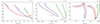 |
Fig. 3. Relative positions of marginally stable circular orbits shown for several values of polytropic parameter n. For n = 3.8 we can see the onset of extremely large polytropes for higher values of parameter σ, since values of the absolute positions ξMSCO are only slightly affected by σ and all remain in the interval (0.8, 2.4). Solid circles show the maximum considered value of sigma σcausal ≡ n/(n + 1). |
The radial profile of the orbital velocity of the circular geodesics that should be relevant in comparison of the polytrope model predictions with the observational data reads
![Mathematical equation: $$ \begin{aligned} v(\xi ) = \left[\frac{-(n + 1)\sigma \xi \frac{\mathrm{d}\theta }{\mathrm{d}\xi }}{1 + \sigma \theta }\right]^{1/2} \left[1 + \frac{(n + 1)\sigma \xi }{1 + \sigma \theta }\frac{\mathrm{d}\theta }{\mathrm{d}\xi }\right]^{-1/2}\, . \end{aligned} $$](/articles/aa/full_html/2025/10/aa54520-25/aa54520-25-eq56.gif) (53)
(53)
Notice that all the functions characterizing the circular geodesics are governed only by the structure function, θ(ξ), being independent of the “mass” structure function ν(ξ). They are influenced only by the parameter ν(ξ1) characterizing the total mass of the polytropic sphere; similarly, the cosmological constant occurs explicitly only in the constant term, λξ12. Of course, the influence of the cosmological constant is implicitly contained in the structure function, θ(ξ), which is a solution of the structure equation depending on the cosmological constant. As is explicitly shown in Stuchlík et al. (2016), the role of the cosmological constant is crucial for extended polytropes that are relevant in our attempt to use them in modeling dark matter halos.
5.1. Trapping polytropes
The analysis of the circular geodesics of the internal polytrope spacetime enables so-called trapping polytropic spheres to be introduced. These are polytropes containing a central region of trapped null geodesics (Stuchlík et al. 2016; Novotný et al. 2017). Since the region of trapped null geodesics is unstable against gravitational perturbations, leading to gravitational collapse forming a central black hole, and is substantially smaller in comparison to the whole trapping polytrope (Stuchlík et al. 2017), the trapping polytropes could potentially serve as an alternative explanation for the existence of supermassive black holes in galaxies observed at redshifts z > 6.
For null geodesics the effective potential takes the form
![Mathematical equation: $$ \begin{aligned} V_{\rm null}(\xi )&= (1 + \sigma \theta )^{-2(n + 1)}\nonumber \\&\quad \times \left\{ 1-2(n + 1)\sigma \left[\frac{\nu (\xi _{1})}{\xi _{1}} + \frac{1}{3}\lambda \xi _{1}^{2}\right] \right\} \frac{L^2}{\mathcal{L} ^2\xi ^2}\, . \end{aligned} $$](/articles/aa/full_html/2025/10/aa54520-25/aa54520-25-eq57.gif) (54)
(54)
The local extrema of this effective potential are given by the condition
 (55)
(55)
which, as expected, corresponds to the loci of simultaneous divergence of the specific energy and specific angular momentum of circular geodesics. These extrema govern the existence of circular null geodesics that in the case of the internal polytrope spacetimes come generally as twins – for properly chosen values of the parameters n, σ, and λ a stable inner (unstable outer) null circular geodesic exists in the trapping polytropes. The null circular geodesics first occur when d2Vnull/dξ2 = 0, implying the condition
![Mathematical equation: $$ \begin{aligned} 3 + \sigma \left\{ 3\sigma \theta ^2 + (n + 1)\xi \left[\frac{\mathrm{d}\theta }{\mathrm{d}\xi }\left(4 + (2n + 3)\sigma \xi \frac{\mathrm{d}\theta }{\mathrm{d}\xi }\right) - \xi \frac{\mathrm{d}^2\theta }{\mathrm{d}\xi ^2}\right]\right. \nonumber \\ \left. + \theta \left[6 + (n + 1)\sigma \xi \left(4\frac{\mathrm{d}\theta }{\mathrm{d}\xi } - \xi \frac{\mathrm{d}^2\theta }{\mathrm{d}\xi ^2}\right)\right] \right\} = 0\, . \end{aligned} $$](/articles/aa/full_html/2025/10/aa54520-25/aa54520-25-eq59.gif) (56)
(56)
We determined by using a computational code the region in the parameter space where the trapping polytropes exist. Numerical calculations reflecting the influence of the cosmological parameter on the trapping polytropes are represented in Figs. 4 and 5. As expected, with increasing parameter λ the restrictions correspond to decreasing polytropic parameter n and decreasing relativistic parameter σ. However, strong differences in restrictions on the trapping polytropes in the σ–n plane arise for the values of λ > 10−5; above this line the results are indistinguishable from the limit λ = 0 case – see Fig. 5. The detailed study of the trapping polytropes in dependence on the cosmological parameter is planned for a future paper. Here we make comments on the application of the results obtained in the limiting case λ = 0 in Stuchlík et al. (2017) on the possibility of gravitational collapse of the trapping region and its consequences. First, we summarize the previous results.
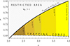 |
Fig. 4. Trapping region in n–σ parameter space. For spatially finite configurations, possible pairs (n, σ) are additionally bounded in dependence on the value of λ (see Fig. 2). |
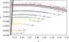 |
Fig. 5. Minimal values of the parameter σ with respect to parameters n and λ for which the trapping phenomenon occurs. Their limitations with respect to the parameter n is set by considered physically plausible values of σcausal and by the requirement of the existence of polytropic configurations (rings at the end of the lines; using depicted scope visible up to λ = 5 × 10⁻⁴). Borderlines for common values of n for cases λ < 10−5 differ only negligibly from the case λ = 0. |
In the case of λ = 0, the regions of the parameter space n–σ corresponding to the trapping polytropes were obtained in Novotný et al. (2017) – the regions start at n = 2.12 and σ = 0.680 and are considered up to n = 4, where the range of the relativistic parameter is 0.667 < σ < 0.8. In Stuchlík et al. (2017) it was demonstrated that in all of these trapping polytropes, the trapping regions are unstable relative to gravitational perturbations and gravitational collapse, leading to the creation of a black hole. The fate of the system of the created black hole and the remaining polytrope depends on the extension of the trapping region in relation to the complete polytrope sphere. If the black hole represents only a minor part of the polytrope, we can expect possible stabilization and modification of the polytrope remnants by rotational effects or other phenomena. On the other hand, if the trapping region represents a relatively large part of the polytrope sphere, we can expect fast collapse of the polytrope remnant onto the created black hole. Detailed analysis in Stuchlík et al. (2017) shows that for polytropes with polytropic index n < 3.5, the ratio of the trapping region extension to the whole polytrope extension is decreasing from 0.1 for n ∼ 2.2 to 0.001 for n ∼ 3.5, indicating possible fast conversion of the whole polytrope to a black hole, while for n ≥ 3.8 the ratio is falling under the value of 10−7 suggesting the possibility of the stabilization of the remaining part of the polytrope. (In the mediate region of polytropes with 3.5 < n < 3.8, the ratio is falling from 10−3 to 10−7 – for details see Stuchlík et al. (2017).) The ratio of mass inside the trapping region to the total mass of the polytrope demonstrates two sections Stuchlík et al. (2017): in the first section, the ratio evolves from 0.55 for n ∼ 2.2 to 0.03 for n ∼ 3.75 suggesting the conversion of the whole polytrope to a black hole, while in the second section the ratio is ∼10−3 for 3.8 < n < 4. The second section is thus interesting for the explanation of supermassive black holes in the active nuclei in the very early galaxy structures.
On the base of the summary of results obtained for the case λ = 0, we are able to give estimates of the influence of the parameter λ presented in our results summarized in Figs. 4 and 5. As the equations governing local extrema of the effective potential of null geodesics, and the extension of the trapping region, do not explicitly contain the cosmological constant, being dependent on λ only implicitly due to the function θ(ξ), we can assume, because of the results obtained above, that for sufficiently low values of the parameter λ extension of the trapping region and the ratio of the mass contained in the trapping region and the total polytrope mass are given with high precision by the analysis done for the λ = 0 case. We can thus conclude that in the physically interesting cases connected with the trapping polytropes having polytrope index 3.8 < n < 4, the relation of the mass Mtr contained in the trapping region and the mass of the whole polytrope mass M, the DM halo mass MHalo is estimated as Mtr/M ∼ Mtr/MHalo ∼ 10−3 as demonstrated in detail in Stuchlík et al. (2017). Numerical calculations for some cases with the inclusion of the sufficiently low cosmological parameter, λ, confirm this expectation of the validity of the creation of supermassive black holes in extremely extended dark matter halos and their clusters. Therefore, we can expect supermassive black holes of mass going from MBH-galaxy ∼ 109 M⊙ in large galaxy halos of mass Mgalaxy ∼ 1012 M⊙ to the black hole mass MBH-cluster ∼ 1012 M⊙ in halos of large galaxy clusters with mass Mcluster ∼ 1015 M⊙. Of course, a more detailed study of the role of parameter λ across the whole region of trapping polytropes is planned for future work. We can expect that with increasing λ the trapping effect will be suppressed as the role of the gravitational repulsion of the vacuum energy increases in comparison with the gravitational attraction of the polytropic fluid that induces the trapping effect and gravitational instability.
5.2. Geodesic structure of the polytropes in dependence on their parameters
We now search for families of general relativistic polytropes that allow the existence of stable circular geodesics, along with possible associated unstable circular geodesics governing the motion of test particles. These geodesics can correspond to the circular motion of baryonic matter in the spacetime background defined by the polytropes.
We give an analysis of the timelike circular geodesics in dependence on the three free parameters of the polytropic models: the polytropic index, n, relativistic parameter, σ, and central density, ρc or, equivalently, the parameter, λ, related to the observationally constrained cosmological constant (vacuum energy) considered in the present paper. Note that the circular geodesics give an illustrative insight into the character of the gravitational field of the internal polytrope spacetime, especially the specific energy of the circular geodesics representing the magnitude of the gravitational binding at a given radius of the polytropic configurations.
We first give the possible types of the behavior of the effective potential that imply classification of the polytrope spacetime according to the character of distribution of the circular orbits across the spacetime. The representative sequences of the effective potential are presented in Fig. 6. The effective potentials are constructed for a polytrope selected to contain all the possible cases of the behavior of the effective potential. Therefore, there are potential curves having one (stable) equilibrium point, two equilibrium points (the inner stable and outer unstable), three equilibrium points (inner and outer stable, mediate unstable), or no equilibrium point. The parameter space of the polytropes can be separated into three regions: the first corresponds to polytropes that only allow for one stable point, having one region of stable circular orbits; the second allows for the existence of two equilibrium points where the region of stable circular orbits is restricted by the limiting outer marginally stable orbit; and the third even allows for three equilibrium points, where two separated regions of stable circular orbits can exist being separated by a region of unstable orbits. The results of computational code for separating the different types of polytropes from the viewpoint of the properties of circular geodesics are presented in Fig. 7; the separation procedure requests very precise calculations because of very small differences in the magnitude of the effective potential local extrema. Therefore, we give the separation in the parameter space for the fixed value of λ = 0.
 |
Fig. 6. Radial profile of the function Veff. Notice the change of its behavior relative to the value of parameter L/ℒ. |
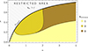 |
Fig. 7. Figure depicting the maximum number of extremes of the function Veff with respect to the value of parameter pair (n, σ). Parameter L (on which Veff is also dependent) has been taken in such a way to maximize this number. |
The representative radial profiles of E, L, and Ω are given later in the discussion of the polytrope properties (in the Zenodo link – A.3, A.4, B.5, and B.6 – specific E(r), L(r) profiles are demonstrated for selected polytropes). Of crucial interest is the mapping of boundaries in the parameter space, separating the polytropes where only the stable circular geodesics exist from those where also unstable circular geodesics are allowed. Of course, from the astrophysics point of view, the regions of stable circular geodesics are only relevant for the motion of matter in dark matter halos. The region of parameters allowing for the existence of marginally stable (and consequently also unstable circular geodesics) is generated by a numerical code, and the results are reflected in Fig. 7.
As expected intuitively, the nonrelativistic polytropes allow only stable circular geodesics across their whole internal spacetime; for the existence of regions of unstable circular geodesics, the relativistic parameter, σ, has to be sufficiently high.
It should be stressed that the radial profiles of the velocity of circular geodesics can be directly related to the velocity profiles observed at galaxies (or galaxy clusters) only at their outer regions. The inner regions may also provide relevant information, but it is important to keep in mind that these regions are affected by the significant contribution of visible, or more generally, standard baryonic matter to the gravitational potential of the galaxy (or cluster). In the case of the trapping polytropes, and their relation to the high-redshift galaxies, an even more complex situation occurs because of both the expected formation of the central black hole, and the lack of observational data that could be improved by the planned space mission ATHENA.
6. Polytrope stability against radial pulsations
In the context of the gravitational instability of the central regions of trapping polytropes against collapse (Stuchlík et al. 2017), it is crucial to test the stability of the polytropes with the vacuum energy described by the cosmological constant in relation to the radial pulsations that can be taken as another relevant test of the polytrope instability. We study the dynamical stability of the polytropes against radial pulsations applying the standard method of Chandrasekhar (1964), modified in Misner et al. (1973) and extended for inclusion of the cosmological constant (Stuchlík & Hledík 2005; Posada et al. 2020). We extend the study of polytrope stability against radial pulsations presented in Posada et al. (2020) to those having the polytropic index n > 3, covering thus the whole region of the trapping polytropes with n ≤ 4.
6.1. Einstein equations governing radial pulsations
In the standard Schwarzschild coordinates (t, r, θ, φ), the spacetime element (1) of the radially pulsating, spherically symmetric polytropic configuration has to be governed by the metric coefficients taken in the general form including the time-dependence
 (57)
(57)
The matter inside the pulsating configuration is assumed to be a perfect fluid, with ρ(r, t) being the energy density and p(r, t) being the isotropic pressure.
The equilibrium (unperturbed) state of the polytrope, about which the configuration pulsations are realized, is the static solution given in the previous section that is characterized by the functions Φ(r), Ψ(r), ρ(r), p(r), and M(r) determined by Eqs. (25)–(30).
The pulsating polytropic configuration (with perturbed quantities depending on time) is determined by the Einstein gravitational equations taking the form
 (58)
(58)
 (59)
(59)
 (60)
(60)
 (61)
(61)
Here, the prime denotes partial derivative with respect to radial coordinate, and the dot denotes partial derivative with respect to time coordinate.
For pulsations of a small amplitude, the metric coefficients, Ψ(r, t) and Φ(r, t), and the thermodynamic variables, ρ(r, t), p(r, t), and n(r, t) (n being the number density of baryons in the fluid), measured in the fluid rest frame, can be described by their small Euler variations,
 (62)
(62)
where the general variable is related to quantities δq ≡ (δΦ, δΨ, δρ, δp, δn). The subscript 0 is related to these variables in the equilibrium state.
The pulsation is governed by the radial displacement, ξ, of the fluid from the equilibrium position
 (63)
(63)
Then the Euler perturbations, δq, are connected to the Lagrangian perturbations, Δq, measured by an observer co-moving with the pulsating fluid by the relation
 (64)
(64)
The pulsation dynamics, i.e., the time evolution of the perturbation function, is governed by the Einstein gravitational equations which have to be combined with the energy-momentum conservation, baryon conservation, and the thermodynamic laws. All the relevant equations have to be “linearized” relative to the displacement from the static equilibrium configuration. The dynamic equation governing the evolution of the fluid displacement ξ(r, t) must be obtained, along with a set of initial-value equations that express the perturbation functions δΦ, δΨ, δρ, δp, and δn in terms of ξ(r, t). The cosmological constant (connected to the vacuum state of the spacetime) is not perturbed, as we do not assume any relation of the cosmological constant (vacuum energy) to matter. We performed the dynamical stability analysis following the method introduced in Chandrasekhar (1964) and developed in Misner et al. (1973), see also (Böhmer & Harko 2005; Stuchlík & Hledík 2005). A detailed derivation of the equations governing the first-order perturbations of polytropes reflecting the influence of the cosmological constant can be found in Posada et al. (2020); here, we give a summary of the perturbation equations and significantly extend calculations and discussion.
6.2. Pulsation dynamics and Sturm–Liouville equation
Introducing a renormalized displacement function (Misner et al. 1973),
 (65)
(65)
the dynamic equation governing the polytrope pulsations takes the form
 (66)
(66)
Here . (,) means a derivation related to the time (radial) coordinate. The functions, W(r), P(r), and Q(r), are determined for the equilibrium polytropic configuration by the relations including the influence of the cosmological constant,
 (67)
(67)
 (68)
(68)
![Mathematical equation: $$ \begin{aligned}&Q \equiv e^{\Psi _0 + 3\Phi _0}\left[\frac{(p_0\prime )^2}{\rho _0 + p_0}\frac{1}{r^2} - \frac{4p_0\prime }{r^3} - (\rho _0 + p_0)\left(\frac{8\pi G}{c^4}p_0-\Lambda \right)\frac{e^{2\Psi _0}}{r^2}\right]\, , \end{aligned} $$](/articles/aa/full_html/2025/10/aa54520-25/aa54520-25-eq72.gif) (69)
(69)
where the adiabatic index, γ, is determined by the relation (for details, see Posada et al. (2020))
![Mathematical equation: $$ \begin{aligned} \gamma = \left(p\,\frac{\partial n}{\partial p}\right)^{-1} \left[n-(\rho + p)\frac{\partial n}{\partial \rho }\right]\, . \end{aligned} $$](/articles/aa/full_html/2025/10/aa54520-25/aa54520-25-eq73.gif)
This γ is not necessarily identical with the adiabatic index related to the equation of state, as is discussed in Hladík et al. (2020).
The boundary conditions guarantee that the displacement function cannot imply a divergent energy density and pressure perturbations at the center of the sphere; therefore, ξ/r is finite for r → 0. The Lagrange variations in the pressure must keep the condition p = 0 at the surface of the polytropic configuration at the radius R. Therefore,
 (70)
(70)
The linear dynamical stability analysis is realized by the standard assumption of the displacement decomposition,
 (71)
(71)
implying a reduction in the dynamic equations to the Sturm–Liouville equation,
 (72)
(72)
with boundary conditions
 (73)
(73)
 (74)
(74)
The Sturm-Liouville equation (73) and the boundary conditions determine eigenfrequencies ωj and corresponding eigenmodes ζi(r), where i = 1, 2, …, n. The stable polytropic configurations have a discrete spectrum of the normal radial modes. The ith mode has i nodes between the center and the surface of the polytrope. The eigenvalue Sturm–Liouville (SL) problem can be represented in the variational form as the extremal values of
 (75)
(75)
determine the eigenfrequencies ωi and the corresponding functions ζi(r) are the eigenfunctions that have to satisfy the orthogonality relation Misner et al. (1973)
 (76)
(76)
The absolute minimum value of Eq. (76) represents the squared frequency of the fundamental mode of the radial pulsations. The negative values correspond to the unstable configurations, as eiωt grows exponentially with time, while the positive values correspond to the configurations stable against adiabatic radial perturbations. Therefore, a sufficient condition for the dynamical instability is the vanishing of the right-hand side of Eq. (76) for a trial function satisfying the boundary conditions (Misner et al. 1973; Chandrasekhar 1964).
The condition ω2 = 0 for the marginally stable configurations enables us to deduce from Eq. (76) a formula giving the critical value of the adiabatic index, γc, assuming that it is constant through the configuration in accord with Chandrasekhar (1964); for a detailed discussion of the issue of the adiabatic index see Hladík et al. (2020). The critical value of the adiabatic index is thus given by the formula
![Mathematical equation: $$ \begin{aligned} \gamma _{\mathrm{c}}&= \left(\int _0^R \frac{e^{\Psi _0 + 3\Phi _0}}{r^2} \left[\frac{(p_0\prime )^2}{\rho _0 + p_0} - \frac{4p_0\prime }{r} - (\rho _0 + p_0)\left(\frac{8\pi G}{c^4}p_0 \right.\right.\right.\nonumber \\&\quad \left.\left. -\Lambda \Big )e^{2\Psi _0}\right] {\zeta }^2\,\mathrm{d} r\right) \Bigg / \left({\int _0^R \frac{p_0}{r^2}e^{\Psi _0 + 3\Phi _0}\zeta {\prime }^{2} \,\mathrm{d} r} \right)\, . \end{aligned} $$](/articles/aa/full_html/2025/10/aa54520-25/aa54520-25-eq81.gif) (77)
(77)
Nevertheless, the Chandrasekhar approach can be generalized, as is demonstrated in the following subsection.
6.3. Dynamical stability of polytropes
The Sturm-Liouville equation can be used to determine the dynamical instability of spherical configurations of perfect fluid with any equation of state. Here, we first present results of the stability study in the special case of the uniform density configurations (see also Böhmer & Harko 2005; Stuchlík & Hledík 2005) and then concentrate on the general polytropic spheres.
In the special case of the polytropes with n = 0, corresponding to spheres with uniformly distributed energy density (Stuchlík 2000; Stuchlík et al. 2016), the metric coefficients can be given by elementary functions and the stability problem can be solved relatively easily. It was demonstrated (Böhmer & Harko 2005; Stuchlík & Hledík 2005) that the instability of the uniform spheres occurs for
 (78)
(78)
For vanishing cosmological constant (λ = 0) the condition reduces to the result presented in (Chandrasekhar 1964):
 (79)
(79)
In the case of the relativistic polytropes, we can directly apply the formulae for the radial profiles of the metric coefficients, the energy density, and the pressure as introduced in Stuchlík et al. (2016). Then the variational Sturm-Liouville equation for dynamical stability of the polytropic spheres with respect to radial pulsations takes, under the assumption of the adiabatic index γ being constant across the sphere, the form
![Mathematical equation: $$ \begin{aligned}&\omega ^2L^2\rho _{\mathrm{c}}c^2 \int _0^{x_1}e^{3\Psi + \Phi }\theta ^n(1 + \sigma \theta ) \bar{\zeta }^2\,\frac{\mathrm{d} x}{x^2} \nonumber \\&=\gamma \sigma \rho _{\mathrm{c}}c^2 \int _0^{x_1} e^{\Psi + 3\Phi }\theta ^{n + 1} \left(\frac{\mathrm{d}\bar{\zeta }}{\mathrm{d}x}\right)^2\frac{\mathrm{d} x}{x^2} -\sigma (n + 1)\rho _{\mathrm{c}}c^2 \nonumber \\&\quad \times \int _0^{x_1}e^{\Psi + 3\Phi }\Bigg \{\theta ^n\frac{\mathrm{d}\theta }{\mathrm{d}x}\frac{4}{x}\left[\frac{\sigma (n + 1)x}{4(1 + \sigma \theta )}\frac{\mathrm{d}\theta }{\mathrm{d}x} - 1\right] \nonumber \\&\quad -2(1 + \sigma \theta )\theta ^n \left(\sigma \theta ^{n + 1}-\lambda \right)e^{2\Psi }\Bigg \}\bar{\zeta }^2\,\frac{\mathrm{d} x}{x^2}\, . \end{aligned} $$](/articles/aa/full_html/2025/10/aa54520-25/aa54520-25-eq84.gif) (80)
(80)
We canceled the subscript 0, as it is not necessary. For the polytropes under consideration, the adiabatic index can be given in the form
 (81)
(81)
which is generally a function of radius.
In the following, we consider the specifics related to the adiabatic index in treating the dynamical stability of polytropes. We apply the approach of our previous paper (Posada et al. 2020), extending its results to values of the polytropic index n > 3 relevant for extremely extended polytropes. We discuss in detail the dependence of the solutions on the parameter λ governing the role of the cosmological constant in relation to the central density of the configuration.
We use a more general approach in comparison with Chandrasekhar’s method (Chandrasekhar 1964) – the adiabatic index in Eq. (81) is considered an effective one, following the method introduced in Merafina & Ruffini (1989):
 (82)
(82)
The stability condition then takes the form
 (83)
(83)
The relation of the radial derivatives of p and Φ is transferred into the form
 (84)
(84)
and the Sturm–Liouville equation (73) can be expressed in the form
 (85)
(85)
where we define
 (86)
(86)
![Mathematical equation: $$ \begin{aligned} Q(x)&\equiv \frac{\rho _{\rm c}\sigma (n+1)\theta ^n e^{\Psi _0 + 3\Phi _0}}{\mathcal{L} ^4 x^2}\left[\frac{\sigma (n+1)}{1+\sigma \theta }\left(\frac{\mathrm{d} \theta }{\mathrm{d} x}\right)^2 + \right. \nonumber \\&\quad - \left.\frac{4}{x}\left(\frac{\mathrm{d} \theta }{\mathrm{d} x}\right) - 2(1 + \sigma \theta )(\sigma \theta ^{n+1}-\lambda )e^{2\Psi _0} \right]\, ,\end{aligned} $$](/articles/aa/full_html/2025/10/aa54520-25/aa54520-25-eq91.gif) (87)
(87)
 (88)
(88)
A short discussion of the dynamical stability of the polytropes with nonzero cosmological constant has been presented in Posada et al. (2020); however, it is restricted to polytropic indexes n ≤ 3. Therefore, the case of very extended trapping polytropes with n > 3.5 was omitted. For this reason we are presenting in this paper a detailed testing with the inclusion of the polytropes with n > 3, considering the polytropic index up to n = 4. We focus on details of the existence of such polytropes, especially on boundaries of so-called forbidden regions concentrated around some special values of the relativistic parameter σ, and on the behavior of the very extended trapping polytropes demonstrating instability against gravitational perturbations leading to gravitational collapse of their central region which were studied in Stuchlík et al. (2017). The discussion is separated for selected values of the cosmological parameter λ = ρvac/ρc relating the vacuum energy density to the central density of the polytrope. We demonstrate that such gravitationally unstable polytropic structures are also dynamically unstable against radial pulsations.
For the calculations, we used the standard trial functions,
 (89)
(89)
yielding
 (90)
(90)
In the most interesting case of very extended trapping polytropes, the cosmological parameter, λ = ρvac/ρc, should be very low, as we expect a large central density of matter; for illustrative reasons we make calculations for appropriately selected values of the cosmological parameter, λ.
The critical value of the adiabatic index can be determined by numerical integration only. We consider values of the repulsive cosmological constant that could clearly demonstrate its role in the stability of polytropic spheres. On the other hand, we study polytropic spheres with a magnitude of the cosmological parameter large enough to enable the existence of stable circular geodesics in the exterior region of the polytropic sphere. The results are given in Fig. 8.
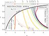 |
Fig. 8. Restrictions on the polytrope parameters. Unified (n–σ) plot for possible finite polytropic configurations distinguished by the cosmological parameter λ. Considered polytropes have the parameter pairs n–σ limited by the σcausal boundary (black line) and the boundaries determined by the static radius given by a chosen λ (thick colored line); monotonically decreasing pressure is expected in the whole interior of the configuration. Thin colored borderlines depict the transition between polytropes stable and unstable against the radial oscillations. For given n the parameter σ needs to be lower than that depicted by this border. For λ < 1/104 these borderlines are all hardly distinguishable from the case λ = 0. They are determined using both trial functions, and the plotted ones represent the more restrictive for the chosen value of λ. Generally, no stable configurations having σ < σcasual and n > 3 exist. A detailed view of the boundaries for lower λ are on the next figure. |
We can see that the trapping region transforms into the forbidden region where no acceptable polytropic spheres can exist due to the effect of the cosmic repulsion. The extension of the polytropes cannot exceed the static radius. For a clear illustration of this effect, and a clear demonstration of the influence of the cosmological parameter λ on the structure and properties of the polytropic spheres, we present the extension of the polytropes as related to the static radius in Fig. 9, where regions of the most extended polytropes are depicted. For large values of the polytropic index (n > 3), the polytropes are unstable against radial perturbations even for large values of λ, including the region of the trapping polytropes where the instability against gravitational perturbations is also present (Stuchlík et al. 2017).
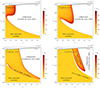 |
Fig. 9. Details of the (n–σ) plane for higher values of n for several values of cosmological parameter, λ. Depicted is the ratio of the radius ξ1 and the static radius ξs ≡ (3ν(ξ1)/2λ)1/3 for the finite configurations. In the plotted region, all considered configurations are unstable to radial perturbations. |
The general discussion of the polytrope properties in dependence on the cosmological parameter is finished. In the following, we fix the vacuum mass density parameter by the relict cosmological constant at ρvac ∼ 10−29 g cm−3 – then the selection of λ uniquely determines ρc, or vice versa.
7. Models of DM halos
In order to test the possibility to model galactic dark matter halos by the general relativistic polytropic spheres in spacetimes with the repulsive cosmological constant, it is useful to express the length and mass scales of the relativistic polytropes in the form adjusted to the astrophysically relevant, galactic conditions. We consider DM halos related to typical galaxies, comparable to the Milky Way, or to extremely large galaxies, or to the clusters of galaxies. The length scale of galactic halos related to typical galaxies, similar to the Milky Way galaxy, is estimated to be 100–200 kpc, while the estimated mass of the halo is considered to be about 1–5 × 10¹² M⊙. Of course, in the case of extremely large and massive galaxies and galaxy clusters, the extension of the halo can increase up to 1 Mpc or slightly more, and the halo mass could be as large as 1015 M⊙ (Ziolkowski 2005).
Therefore, we give the length scale as
![Mathematical equation: $$ \begin{aligned} \mathcal{L} = 1.061 [\sigma (n + 1)]^{1/2}\frac{(10^{-20}\,\mathrm{g\, cm^{-3}})^{1/2}}{\rho _{\mathrm{c}}^{1/2}}\,100\,\mathrm{kpc}\, , \end{aligned} $$](/articles/aa/full_html/2025/10/aa54520-25/aa54520-25-eq95.gif) (91)
(91)
and the mass scale as
![Mathematical equation: $$ \begin{aligned} \mathcal{M} = 2.217 [\sigma (n + 1)]^{3/2}\frac{(10^{-20}\, \mathrm{g\, cm^{-3}})^{1/2}}{\rho _{\mathrm{c}}^{1/2}}\,10^{18}\, \mathrm{M_{\odot }}\, . \end{aligned} $$](/articles/aa/full_html/2025/10/aa54520-25/aa54520-25-eq96.gif) (92)
(92)
The polytropic spheres with given mass and length scales are precisely determined by the solution of the structure equations given by the radial coordinate ξ1(n, σ, λ) and the related mass parameter ν(ξ1)(n, σ, λ). Generally, the exact solutions can strongly modify the length and mass scales; however, for nonrelativistic dark matter with σ ≪ 1, the length and mass scales are decisive. Then we can obtain the polytrope sphere with extension and mass in agreement with the galactic halo estimates for [σ(n + 1)] < 10−4. However, the central density of such polytropes has to be very small.
7.1. Rough mapping based on scaling estimates
We first give the estimates related to the extension and mass scales for the limiting DM halos under consideration. At the lower end, we consider their extension R ∼ 100 kpc and mass M ∼ 1012 M⊙, to the upper end where R ∼ 1 Mpc and M ∼ 1015 M⊙.
Rough estimates on the extension scale give the relation
 (93)
(93)
where
 (94)
(94)
while the rough mass estimate relation takes the form
 (95)
(95)
For the lower-end DM halos (M ∼ 1012 M⊙), we then find the estimates for the relativistic parameter and central density,
 (96)
(96)
For the upper-end CDM halos (M ∼ 1015 M⊙), we find the estimates
 (97)
(97)
Clearly, the rough estimates based on the length and mass scaling predict only strongly nonrelativistic, σ < 10−4, and highly diluted fluid with central density ρc ∼ 10−22 g cm−3. Of course, our estimates are relevant for the fluids with nonrelativistic (first) regime of the behavior of the dimensionless polytrope parameters ξ1 and ν(ξ1).
7.2. Exact mappings based on exact models of the polytropic spheres
A detailed analysis of the correspondence of the extension and mass of the general relativistic polytropic spheres and the observationally restricted DM halos was realized by numerical methods using the exact solutions of the polytrope structure equations. In the matching procedure for the exact models of polytropes, we used the extension R = ℒξ1 and mass M = ℳν(ξ1). We separated the procedure of the exact mapping of the polytropic spheres into two cases, corresponding to the two regimes giving extremely extended and massive polytropic spheres. The first one is related to the nonrelativistic polytropic fluid with the relativistic parameter σ < 10−3 when we expect the extended configurations with a very low central density, predicted by the rough scale estimates. The second case corresponds to the very extended polytropic configurations with relativistic parameter σ very close to the critical values, when the dimensionless radius ξ1 can be extremely large.
7.2.1. Mapping in the nonrelativistic regime
Recall that in the case of nonrelativistic polytropes we model the CMD halos. In Figure 10 the constant values of the polytrope extension R and mass M are given as the functions of the parameters σ and ρc that uniquely determine also the cosmological parameter λ. Here we follow the first regime, the case of nonrelativistic polytropes, σ < 10−3, with the whole range of considered polytropic indexes for which the critical function λcrit was constructed. In the parameter space σ–ρc we give the regions allowing for polytropic spheres with an extension and mass comparable to those of the observed large galaxies and the galaxy clusters for the polytropic indexes n = 0.5, 1, 1.5, 2, 2.5, 3, 3.5, 4, and 4.5. In all nine cases, the allowed regions were numerically computed and constructed for the galaxy-like regime with 100 kpc ≤R≤ 200 kpc, 1012 M⊙ ≤ M ≤ 5 × 10¹² M⊙, and the cluster-like regime with 1 Mpc ≤R≤ 5 Mpc, 1015 M⊙ ≤ M ≤ 5 × 10¹⁵ M⊙.
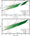 |
Fig. 10. Allowed regions of galaxy-like and cluster-like polytropes in the nonrelativistic regime. The figure shows the polytrope extension, R, and mass, M, at the edges of the selected intervals R = 100–200 kpc and M = 1–5 × 10¹² M⊙ (top figure) and R = 1–5 Mpc & M = 1–5 × 10¹⁵ M⊙ (bottom figure). We are drawing only the extensions R and M for the polytropic index n = 0.5 (4 lines). However, the “polygon shape” intersections are demonstrated for n = 0.5 up to n = 4.5 with step size 0.5. The intersection for n = 0.5 is the leftmost one, for n = 1.0 the intersection region is located to the right of the previous one, and so on. Also, the non-integers n are filled with single hue color (increasing the hue for higher polytropic index) for a better overview. The two vertical lines correspond to the critical value ρcrit(n; σ), i.e., the λcrit(n; σ) (see Section 4) for two polytropic index (4.5,3.0). The configurations for the particular n can only exists on the right side of the curve. The dots represent the selected points for the polytropic spheres whose profiles are given in the next section. |
The results reflected in Fig. 10 demonstrate for both the galaxy-like and cluster-like allowed regions surprisingly large scatter of the regions in both the parameters σ and ρc from their values predicted by the rough estimates based on the extension and mass scales. The scatter is strong especially in the case of the central density. Such a scatter is caused by the significant dependence of the dimensionless solutions ξ1 and ν(ξ1) of the polytrope structure equations on the polytropic index n, shown explicitly in Stuchlík et al. (2016). Generally, in both the galaxy-like and cluster-like regimes the allowed regions are shifted to larger values of both σ and ρc with increasing polytropic index n.
The allowed regions for the galaxy-like polytropes have the relativistic parameter in the interval of 10−7 < σ < 10−5, symmetric around the rough estimate σ ∼ 10−6, but the central density varies in the interval 10−26 g cm−3 < ρc < 10−21 g cm−3 that is shifted to the lower densities from the rough estimate ρc ∼ 10−23 g cm−3. Notice that the allowed regions of polytropes with n ≤ 2.5 must have ρc < 10−24 g cm−3 and σ < 0.6. On the other hand, the n = 4.5 polytropes must have ρc > 10−23 g cm−3 and σ > 10−6. We shall see in the next section that the density and mass radial profiles of the polytropes belonging to the allowed regions differ significantly for different values of n, indicating large variability for matching the observed velocity curves.
The allowed regions for the cluster-like polytropes have the relativistic parameter in the interval of 10−5 < σ < 10−3, which is again symmetric around the rough estimate σ ∼ 10−4. However, the central density varies in the interval 10−27 g cm−3 < ρc < 10−21 g cm−3 that is shifted to the lower densities from the rough estimate ρc ∼ 10−22 g cm−3 even more significantly than in the case of galaxy-like polytropes. In fact, the upper limit on the central density in the case of the n = 4.5 cluster-like polytropes is at the same value as for the galaxy-like polytropes, but the relativistic parameter σ differs by two orders. Notice that in the case of the n = 0.5 cluster-like polytropes, the central density of such extremely extended structures has to be as small as ρc ∼ 5 × 10⁻²⁸ g cm−3, while σ < 10−5.
7.2.2. Mapping in the relativistic regime
Recall that in the relativistic regime we model non-cold DM halos; for example, the WDM halos. In Figure 11 the constant values of the polytrope extension R and mass M are given as the functions of the parameters σ and ρc in the second regime, for the vicinity of the critical values of the relativistic parameter σ, in the case of the polytropic spheres with the polytropic indexes n = 3.5, 4, 4.5. As in the previous case of the nonrelativistic regime, the allowed regions were numerically constructed for the galaxy-like regime with 100 kpc ≤R≤ 200 kpc, 1012 M⊙ ≤ M ≤ 5 × 10¹² M⊙, and the cluster-like regime with 1 Mpc ≤R≤ 5 Mpc, 1015 M⊙ ≤ M ≤ 5 × 10¹⁵ M⊙. The numerical procedure requests very precise methods as we are generally searching in extremely narrow regions of the parameter space σ–ρc, and in the regions where the dimensionless solutions for the polytropes behave in a non-standard way in the vicinity of the critical values of the parameter σ.
Figure 11 represents a general overview of the search for the allowed regions. Because of the general overview, details cannot be presented here, with the exception of some special cases when the allowed regions are sufficiently extended. The detailed shape of the allowed regions will be in these cases presented in the next section along with the representative radial profiles of the density, mass and metric coefficients of the internal polytrope spacetime.
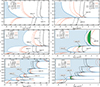 |
Fig. 11. Allowed regions of galaxy-like (left column) and cluster-like (right column) polytropes in the relativistic regime. Dependence of the polytrope extension R and mass M on the parameters σ and ρc. For the polytropic indexes n = 3.5, 4.0, 4.5 (from top to bottom) we highlight the regions of later interest with a letter and number (the letter A is used for the galaxy-like polytropes, while the letter B is used for the cluster-like polytropes). Furthermore, the function ρcrit is shown, where the shaded area is the area of nonexistent configurations for particular n. |
For the n = 3.5 polytropes, there exist two narrow allowed regions of the galaxy-like type (denoted as A1, A2) and two narrow allowed regions of the cluster-like type (denoted as B1, B2), all of them in the vicinity of the critical σ1 (n = 3.5). For the n = 4 polytropes, two galaxy-like narrow allowed regions, A1 and A2, exist around the first critical point σ1 (n = 4), and two narrow allowed regions, A3 and A4, exist around the second critical point σ2 (n = 4). Further, two cluster-like narrow allowed regions, B1 and B2, exist around the first critical point σ1 (n = 4), while one extended allowed region B3 exists under the second critical point σ2 (n = 4) and the other extended allowed region B4 exists above this critical point. For the n = 4.5 polytropes, two galaxy-like narrow allowed regions, A1 and A2, exist around the first critical point σ1 (n = 4.5), and two narrow allowed regions, A3 and A4, exist around the second critical point σ2 (n = 4.5). One narrow allowed region A5 exists near the third critical point σ3 (n = 4.5), and one allowed region A6 exists between the critical points σ3 (n = 4.5) and σ4 (n = 4.5). One narrow cluster-like allowed region B1 is located near the critical point σ1 (n = 4.5), and an extended allowed region B2 is located between the critical points σ1 (n = 4.5) and σ2 (n = 4.5). No other allowed regions were found for the n = 4.5 polytropes near the higher order critical points of the relativistic parameter existing for this kind of polytrope.
8. Radial profiles of density, pressure, and metric coefficients in selected polytropic spheres
We give the radial profiles of the energy density, pressure, mass, and metric tensor coefficients for typical polytropic spheres with polytrope parameters taken from the central part of the galaxy-like and cluster-like allowed regions selected by the previous procedure for all the considered values of the polytropic index n in both the nonrelativistic and relativistic regimes of the fitting procedure. We thus obtain the characteristic radial profiles of density, pressure and metric coefficients related to all the polytropic spheres that could potentially represent the DM halos due to their extension and mass.
The polytropic spheres are governed by the structure functions θ(ξ) and ν(ξ) of the dimensionless coordinate ξ, by the length scale ℒ and the mass scale ℳ. Their extension reads R = ℒξ1 and gravitational mass M = ℳν(ξ1) = c2ℒσ(n + 1)ν(ξ1)/G. We obtain the polytrope radial profiles using Eqs. (25), (26), (27), (28), (29).
We again separate our discussion according to the fitting regime. While considering the galaxy-like and cluster-like polytropic spheres in the nonrelativistic regime, we keep the selection of the parameters σ and ρc in the allowed regions to obtain in both cases polytropes with similar dimensionless characteristics ξ1 and ν1 = ν(ξ1) for a fixed polytropic index, n.
8.1. Profiles of polytropes in the nonrelativistic regime
We first constructed the radial profiles of the nonrelativistic polytropic spheres when all the polytropic indexes 0 < n ≤ 4.5 can be relevant. For each considered n, we selected typical values of the other parameters characterizing the polytropes, σ and ρc, corresponding to the center of the allowed regions obtained by the previous numerical procedures fixing the radius and mass of the polytropic spheres. The results are presented for the selections obtained for the nonrelativistic polytropes with σ < 10−3. We give the results separately for the polytropic spheres related to typical galaxies, keeping them nearly equal for all values of n to the extension R ∼ 115 kpc and mass M ∼ 2.6 × 10¹² M⊙, and for the polytropic spheres corresponding to typical clusters of galaxies, keeping them for all values of n the extension R ∼ 1100 kpc and mass M ∼ 2 × 10¹⁵ M⊙. For nonrelativistic polytropic spheres, a special scale is introduced to represent the metric coefficients, since they remain very close to unity in these configurations. The selected parameters are summarized for both galaxy-like and cluster-like polytropes in Table 1.
Notice that in the nonrelativistic regime the allowed regions depend rather smoothly on the polytropic index, and the required extension and mass parameters. Extension to modified values of R and M is straightforward.
We can make a short comparison of our results related to galaxies with results of previous papers connected with nonrelativistic models of galaxies. For polytropic spheres having n ≤ 1, the profiles are similar to those presented in Böhmer & Harko (2007), where polytropes with n = 1 were studied, and the rotational curves were fit for dwarf galaxies. For n > 1 (and especially for n > 3) the profiles are similar to those presented in Saxton & Ferreras (2010) where large galaxies were fit.
8.1.1. Galaxy-like profiles
For the scales related to the polytropic spheres that could represent galaxies, the characteristic radial profiles are presented in Appendix A.1 for each of the considered polytropic indexes that were used in the fitting procedure for the nonrelativistic polytropes. We can immediately see the crucial influence of the polytropic index n in the radial profiles of all the characteristic quantities. For low values of the index, n ≤ 1, density and pressure (mass) slowly decrease (increase) up to the polytrope edge, and the metric coefficient gtt also slowly decreases up to the edge. Starting from the n = 1.5 polytropic spheres, the decrease in density and pressure (increase in mass) gets sharper with increasing n, and a local minimum of the gtt radial profile occurs, getting deeper and more shifted to the polytrope center with increasing n. For the polytropes with n > 3, the mass of the polytrope is concentrated in the central regions and the density (pressure) rapidly drops to very low values.
8.1.2. Cluster-like profiles
For the scales related to the polytropic spheres that could represent clusters of galaxies, the characteristic radial profiles are presented in Appendix A.2 for each of the considered polytropic indexes, for which the fitting procedure has been realized. The character of the radial profiles in dependence on the polytropic index n is the same as in the case of the galaxy-like typical polytropes, as can be expected due to the same dimensionless characteristics of the polytropes. Again, the uniformity of the energy density and mass distribution across the polytropic sphere strongly decreases with increasing n. Also, the gravitational potential well given by the metric coefficient gtt has a similar character for galaxy-like configurations; however, it is deeper for the cluster-like configurations. Thus, the relativistic effects can be stronger in this case.
8.1.3. Variability across the allowed region
In order to demonstrate the role of the variations in the parameters σ and ρc across the allowed regions, we constructed the polytrope profiles for the special selection of polytropic indexes n = 0.5, 1.5, considering for comparison the radial profiles of the polytropic characteristic functions for the parameters σ and ρc with values reflecting the extension of the allowed region for galaxy-like polytropes. Therefore, the parameters were taken from the four corners of the allowed regions. The resulting radial profiles are presented in Fig. 12. (For the cluster-like polytropes, the results are of the same character.)
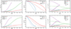 |
Fig. 12. Radial profiles of the mass, ν (left column), energy density, ρ (middle column), pressure, P (middle column), and metric coefficients, gtt, grr (right column), constructed for the parameters σ and ρc on the edges of the allowed regions. The first row of the figure corresponds to the polytropic sphere with n = 0.5, second row corresponds to n = 1.5 polytropes. For better visualization of the metric coefficients we introduced the special scale convenient for the nonrelativistic configurations. |
We can see that the qualitative character of all the profiles remains the same for all four selected limiting points of the allowed regions. Only the mass scale and the polytrope extension are modified accordingly. Of course, the height of the gravitational potential reflected by the metric coefficient gtt is different in the selected polytropes.
8.2. Profiles of polytropes in the relativistic regime
In the case of the relativistic polytropic spheres that could represent large galaxies or clusters of galaxies, only the polytropic indexes n > 3.3 are allowed. For the selections obtained in the second regime of relativistic polytropes with near-critical values of the relativistic parameter σ ∼ σcrit, we separate the discussion according to the considered values of the polytropic index: n = 3.5, 4, and 4.5. Because of the rather complex form of the allowed regions of the parameter space σ–ρc, selected by the fitting procedure on the extension and mass of the polytropes, we restrict again our attention to just one choice of the parameters σ and ρc in each selected allowed region.
For polytropes of the relativistic regime, we can see that the matching of the parameters σ and ρc for various values of R and M is non-trivial and strongly dependent on the polytropic index n > 3.3. Moreover, we also observe an extremely large spread of the central density between various allowed regions. In some allowed regions, a very small central density is implied by the matching procedure, say ρc ∼ 10−16 g cm−3, while in a neighboring one, a very large central density is required, say ρc ∼ 10−2 g cm−3.
For each of the selected values of the polytropic index n = 3.5, 4, 4.5, and each of the corresponding A,B regions of the σ and ρc parameters, we choose typical values of these parameters that we use in the construction of velocity profiles of the circular geodesic motion in the related polytropic spheres. Usually, the regions A and B are concentrated in the vicinity of the critical points σcrit(n), but there also exists an important exception, namely B4 occurring for n = 4 case, where the extension of σ parameter is very large, allowing even for the existence of the so-called trapping polytropes whose astrophysical relevance is exposed in Stuchlík et al. (2017). In all the considered cases, we also depict (in blue) the region forbidden by the critical value of λ, λcrit, by the curve ρcrit(n, σ) defined by Eq. (36).
8.2.1. Profiles of polytropes with n = 3.5
Now all the selected allowed regions are related to the single critical point of the relativistic parameter, and we always choose σ in its close vicinity. The selected values of the parameters σ and ρc are given in Table 2 for both the galaxy-like and cluster-like polytropes. The resulting polytrope radial profiles are demonstrated in the left column of Fig. B.1 for the galaxy-like polytropes and in the right column of Fig. B.1 for the cluster-like polytropes. In the left columns of these figures, we present details of the corresponding polytrope allowed regions. In the n = 3.5 polytrope case, all the allowed regions are closely related to the critical relativistic parameter.
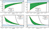 |
Fig. 13. Allowed regions for the n = 3.5 galaxy-like (A1 and A2 regions; left column) and cluster-like (B1 and B2 regions; right column) polytropic spheres. The corresponding radial profiles for the selected values (see Table 2), depicted here by the black dots, are given in Fig. B.1. |
As was intuitively expected, all the extended relativistic polytropes have an extremely large dimensionless radius, ξ1, but the dimensionless mass parameter, ν1, can be both large and small.
We can immediately observe a significant difference in the behavior of the radial profiles in the cases A1 and B1 in comparison to the cases A2 and B2. The A1 (B1) polytropes can be characterized as extremely concentrated ones. All their mass is essentially concentrated in the central region, being essentially constant across the whole polytropic configuration. This is reflected also by the behavior of the metric coefficient 1 − gtt that steeply increases from the center. For the A2 (B2) polytropes, we observe qualitatively different behavior in comparison to the extremely concentrated polytropes, where the energy density is not decreasing so steeply and mass increases along the whole configuration. The gravitational potential well, represented by the metric coefficient 1 − gtt demonstrated a rather complex behavior with one local maximum followed by a local minimum. In such extended relativistic polytropes, their mass is distributed along the whole configuration. Notice that the extremely concentrated polytropes have their mass parameter ν1 < 1, while the spread polytropes have a relatively large mass parameter, ν1 > 10.
8.2.2. Profiles of polytropes with n = 4
The selected allowed regions are related to the two critical points of the relativistic parameter. The selected values of the parameters σ and ρc are given in Table 3 for both the galaxy-like and cluster-like polytropes. The resulting polytrope radial profiles are demonstrated in the right column of Fig. 14 for the galaxy-like polytropes (four regions A1–A4), and of Fig. B.2 for the cluster-like polytropes (four regions B1–B4). In the left columns of these figures, we present details of the corresponding polytrope allowed regions. Notice that the B4 region is distributed between the second critical point of σ parameter and its causal limit σ = 0.8.
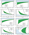 |
Fig. 14. Allowed regions of galaxy-type A (A1–A4, right column) and cluster-like B (B1–B4, left column) for polytropic spheres modeled using n = 4.0. The corresponding radial profiles for the selected values (see Table 3), depicted here by the black dots, are given in Fig. B.1 |
All the extended relativistic polytropes again have an extremely large dimensionless radius, ξ1, while the dimensionless mass parameter, ν1, can be both large and small. There is the standard distribution of the galaxy-like polytropes, as the A1 and A3 polytropes are the typical extremely concentrated polytropes with low parameter ν1, while the A2 and A4 polytropes are the typical spread polytropes with large parameter ν1. However, the cluster-like polytropes demonstrate a non-standard behavior. The B1 polytrope is a typical extremely concentrated one, with very small ν1 < 1, and the B2 polytrope is a typical spread polytrope with large ν1 ∼ 100. On the other hand, the polytropes B3 and B4 demonstrate irregular behavior as they are strongly concentrated, but not extremely. They exhibit relatively large dimensionless mass parameter ν1 ∼ 6 for B3 and ν1 ∼ 70 for B4, but the radial profile of the metric coefficient 1 − gtt shows no local extreme. Notice that both B3 and especially B4 are largely extended in the relativistic parameter σ and in the case of B4, σ reaches the regions where the polytropic spheres contain zones of trapped null geodesics where fast gravitational instabilities could be relevant, as is shown in Stuchlík et al. (2017).
8.2.3. Profiles of polytropes with n = 4.5
The allowed regions are related to three critical points of the relativistic parameter. The selected values of the parameters σ and ρc are given in Table 4 for both the galaxy-like and cluster-like polytropes. There are five allowed regions for the galaxy-like polytropes, but only two of them for the cluster-like polytropes. The A1, A2 regions are related to the first critical point of σ, the regions A3, A4 are related to the second critical point and the A5 region relates to the third critical point. The A6 region is of special character as it is not representing an allowed region but serves as an example of the situation where the conditions for the extension and mass of the polytrope have no intersection giving an allowed region – see Fig. 15.
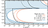 |
Fig. 15. Close-up of the region A6 for the polytropic sphere n = 4.5 representing a galaxy-like scheme. Here the set conditions for R and M have no common region. |
The resulting polytrope radial profiles are demonstrated in the right column of Fig. 16 for the galaxy-like polytropes (five regions A1–A5), and of Fig. 17 and Fig. B.4 for the cluster-like polytropes (two regions B1–B2). The left columns of these figures introduce the detailed shape of the corresponding polytrope allowed regions.
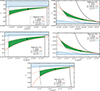 |
Fig. 16. Details of the allowed regions A1–A5 for the polytropes with index n = 4.5. The corresponding radial profiles for the selected values (see Table 4), depicted here by the black dots, are given in Fig. B.3. |
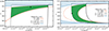 |
Fig. 17. Details of the allowed regions B1–B2 for the polytropes with index n = 4.5. The corresponding radial profiles for the selected values (see Table 4), depicted here by the black dots, are given in Fig. B.4. |
All the extended relativistic polytropes again have an extremely large dimensionless radius, ξ1, while the dimensionless mass parameter, ν1, can be both large and small. In the group of the galaxy-like polytropes, the A1 and A3 polytropes are the typical extremely concentrated polytropes, but for the A3 case the mass parameter is rather high, ν1 ∼ 21. On the other hand, the polytropes A2, A4 and A5 are of the irregular type, having large values of ν1 ∼ 103. The B1 polytrope is a typical extremely concentrated one, with very small ν1 < 1, and the B2 polytrope is an irregular one with large ν1 ∼ 37.
9. Velocity curves in the selected polytropic spheres
For the selected polytropic spheres that could be considered as potential DM halo models, we also construct the model of the velocity curves of stars orbiting in the galactic plane. For this purpose, we give the velocity radial profiles of the circular geodesics in the equatorial plane of the polytrope internal spacetime. In the case of the polytropic spheres, the metric coefficients are constructed numerically; therefore, the velocity radial profiles of circular geodesics will also be determined numerically and roughly compared to the observed velocity profiles.
9.1. Velocity radial profiles
For the selected polytropic spheres that could serve as the DM halo models, we give the specific energy and specific axial angular momentum radial profiles in Appendix A for the case of nonrelativistic polytropes (first regime of fitting procedure), covering thus both the galaxy-like polytropes and the cluster-like polytropes, and in Appendix B for the relativistic polytropes (second regime).
We can see that in the nonrelativistic polytropes the flatness of the specific energy radial profile increases with decreasing polytropic index n. In all the cases, the lowest energy is at the center, giving the binding energy of the circular geodesics. The binding energy increases with increasing n, and it is substantially higher for the cluster-like polytropes in comparison with the galaxy-like ones if n is fixed. In the relativistic extended polytropes, the specific energy radial profile decreases extremely fast near the center. The binding energy increases with increasing n, and it is larger for the cluster-like polytropes in comparison to the galaxy-like polytropes.
We constructed the representative radial profiles of the velocity measured by distant observers and related to the circular geodesics inside the selected polytropic spheres that could represent the CDM halos in large galaxies or galaxy clusters. As in the previous sections, we separate the construction of the velocity radial profiles for the nonrelativistic and relativistic polytropic spheres.
9.1.1. Nonrelativistic polytropes
The velocity radial profiles of the circular geodesics are represented in Fig. 18 for all the considered values of the polytropic index, namely n = 0.5, 1, 1.5, 2, 2.5, 3.0, 3.5, 4, 4.5. We give them for both the galaxy-like polytropes and the cluster-like polytropes.
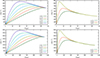 |
Fig. 18. Velocity profiles of the galaxy-like (first row) and the cluster-like (second row) cases for the nonrelativistic polytropes. |
We can see that the nonrelativistic polytropes with n > 1.5 give velocity profiles with a local maximum. For the polytropes with n > 3 the profiles behind the maximum have essentially Keplerian character, excluding them qualitatively as candidates for the galactic halos. However, for the polytropes with 1.5 ≤ n ≤ 3, the profiles have quasi-Keplerian character in the outer regions behind the maximum, being sufficiently flat to enable their consideration as potential candidates for the galactic halos. Moreover, for the polytropes with n < 1.5, the rotational velocity radial profiles are purely increasing with radius and can be considered as candidates for halos of dwarf galaxies.
9.1.2. Relativistic polytropes
In this case, we give the velocity radial profiles separately for the three considered cases of polytropic index n = 3.5, 4, 4.5. In the case of the polytropes with n = 3.5, the velocity profiles are illustrated in Fig. 19 (left column) where we consider the galaxy-like polytropes, and in Fig. 19 (right column) for the cluster-like polytropes. In both cases, there are two regions of the relativistic parameter σ that should be considered. The selected parameters σ, ρc are listed in Table 2.
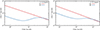 |
Fig. 19. Velocity profiles for the polytropic spheres with the index n = 3.5, related to the large galaxies (left column) and clusters of galaxies (right column). |
For polytropic spheres with n = 4.0, we followed the previous case of n = 3.5, but in this case there are four regions of the relativistic parameter that have to be considered. The selected parameters, σ, ρc, are listed in Table 3. The results are given in Fig. 20.
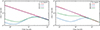 |
Fig. 20. Velocity profiles for the polytropic spheres with the index n = 4.0, related to the large galaxies (left column) and clusters of galaxies (right column). |
For polytropic spheres with n = 4.5, the situation is more complex; there are six regions of interest. The selected parameters, σ, ρc, are listed in Table 4. The resulting velocity profiles are illustrated in Fig. 21.
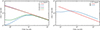 |
Fig. 21. Velocity profiles for the polytropic spheres with the index n = 4.5, related to the large galaxies (left column) and clusters of galaxies (right column). |
The extremely concentrated relativistic polytropes have strongly decreasing velocity profiles and can be excluded as candidates for the galactic halos. However, the spread relativistic polytropes demonstrate humpy velocity profiles that are very flat at the outer regions and could thus be considered as possible candidates for the halos.
10. Simple tests of applicability of the polytrope rotational velocity profiles
In order to test the polytropic spheres as possible models of galactic or galaxy cluster halos, we used the observational data of velocity profiles obtained for individual galaxies (clusters) and matched the data using the velocity profiles related to the polytropic spheres in combination with the velocity profiles related to the galaxy disk (bulge) or gas connected to them. Such detailed matching procedures are, of course, rather complex and time-consuming, and we plan them for a future paper. Here we realize, as a simple preliminary test of our models, a comparison of the velocity profiles predicted by the polytropic models with the velocity profiles determined by the standard approximate models of the DM halos applied in some of the previous studies of matching the observational data related to large galaxies and galaxy clusters4.
In order to test our polytropic spheres, we apply the obtained geodesic rotational velocity radial profiles of the polytropes from the regions of allowed, restricted from above by the influence of the cosmological constant on the polytrope extension and mass, and from below by the extension of the strong influence of the galaxy disk. Note that the polytrope sphere in regions corresponding to the dominance of the galaxy disk should be applied in the direct matching to the observational data.
10.1. Galaxy case
In order to simplify the testing of our results, we make a comparison to the results obtained by the standard approximate models of the CDM galaxy halos. We take the two frequently used models, namely the Navarro–Frenk–White (NFW) density profile Navarro et al. (1997) and a core model with the density profile proposed by Burkert (1995), using the velocity profiles corresponding to their contribution in matching the observational data. A similar approach is applied in Cabral-Rosetti et al. (2004).
The NFW density profile is given by the relation Navarro et al. (1997)
 (98)
(98)
where X = R/h, and ρ0 is the representative (scale) density and h is the scale radius of the CDM halo. The masses within radius R and the circular rotation velocity profile, vNFW, are given by the relations
![Mathematical equation: $$ \begin{aligned} M_{\rm NFW}(R)&= 4\pi \rho _0 h^3 \left[\ln \left(1 + X\right) - \frac{X}{1 + X}\right],\end{aligned} $$](/articles/aa/full_html/2025/10/aa54520-25/aa54520-25-eq103.gif) (99)
(99)
 (100)
(100)
For the matching procedure we have to choose the scale factors ρ0 and h. For our testing of the polytrope spheres we used the results obtained for the galaxy M33 in the paper of Corbelli et al. (2014). Note that in the mentioned paper the authors obtained the characteristic value of the so-called concentration parameter c = (9.5 ± 1.5) and the value of the virial mass Mvir = (4.3 ± 1.0) 1011 M⊙. We have to relate the mass of our polytrope spheres to this virial mass.
The Burkert density profile is given by
 (101)
(101)
where the parameter Y = R/RB and ρB; 0 is the dark matter density of the core; the characteristic radius RB means the core radius. The rotational velocity radial profile related to the Burkert density profile then reads
 (102)
(102)
For the matching procedure, we again used the M33 galaxy study presented in Corbelli et al. (2014).
In Corbelli et al. (2014), the NFW or Burkert halo velocity profiles were combined in the standard Newtonian framework with the velocity profiles related to those corresponding to the galaxy disk (bulge) to match the observational data. Here we only matched the polytrope velocity radial profiles to the velocity profiles related to the NFW and Burkert density profiles obtained for the halo of the galaxy M33. In this way, we overcame the difficulty of mixing the influence of our polytrope models that are fully general relativistic with the influence of the visible parts of the galaxy due to a simple comparison of the velocity curves of our polytrope model with the velocity curve given by the NFW (Burkert) model of the density profile. Both the velocity profiles are related to the distant (Newtonian) observers. In the matching procedure, we used as free parameters the polytrope index, n, and the relativistic parameter, σ, realizing the matching for the case of the M33 galaxy in the interval of radii 40–200 kpc.
The results of the matching procedure of the velocity curves of our polytrope model with both velocity curves given by the NFW and Burkert density models are represented in Fig. 22. To obtain significant matches, the region from 0 to 40 kpc – where the influence of the galactic disk dominates – must be excluded from the matching procedure. We therefore compare only the regions where the velocity contribution from the dark matter halo dominates.
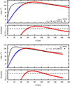 |
Fig. 22. Best match of the polytrope velocity profiles (circles) to the velocity profiles related to the NFW model (top; solid line) and the Burkert model (bottom; solid line) with our best polytrope sphere velocity profiles (circles). The blue circles in both cases represent the points not included in the matching procedure, while the red ones are included. For completeness, we also include the residuals in both cases in dependence on the radius. |
The best match to the NFW model is obtained for the polytropic sphere with the polytropic index n = 2.8 and the relativistic parameter σ = 7.05 × 10⁻⁸. In this case, we obtain the total halo mass M = 3.4 × 10¹¹ M⊙, which is in good correspondence with the mass obtained by Corbelli et al. (2014), i.e., Mh = (4.3 ± 1.0)×1011 M⊙. In the case of the Burkert profile, we found the best match for the polytrope having n = 3.1 and σ = 5.09 × 10⁻⁸, which implies the total polytrope mass M = 1.97 × 10¹¹ M⊙. We see that in both cases the best match is given by the nonrelativistic polytropic configurations, with the polytropic index close to n = 3.
10.2. Cluster case
To test our polytropic spheres in modeling the halos of galaxy clusters, we used the previous study related to the rotational motion in galaxy clusters (Manolopoulou & Plionis 2016). In this work, the authors used for their validation test a virialized cluster with a mass of 4 × 10¹⁴ M⊙, radius Rcl = 1 Mpc and core radius Rc = 0.1 Mpc. The density radial profile of the cluster is represented by the distribution proposed in King (1962), which reads
 (103)
(103)
where ρK; 0 is the central density of the cluster and its value is obtained by using the mass, Mcl, given by the relation
 (104)
(104)
By assuming the cluster is virialized, the rotational velocity profile, vK, is given by
 (105)
(105)
We again compare the velocity curves related to the distant Newtonian observers.
The results of the matching procedure are presented in Fig. 23. We found that in this special case the matching is possible in two regimes: for the nonrelativistic polytropes where the best match is obtained for the polytrope with n = 4.2 the relativistic parameter σ = 1.63 × 10⁻⁵, and for the relativistic polytropes of the spread kind where the best match is obtained for the polytrope with n = 4 the relativistic parameter σ = 0.357.
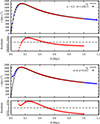 |
Fig. 23. Best match of the polytrope velocity profiles (circles) to the velocity profiles related to the King velocity profile vK (line) is given for the nonrelativistic polytropic sphere (top) and the relativistic polytrope of the spread kind (bottom). The red dots are the points included for the matching procedure, while the blue points are not included. We also show the residuals for monitoring of the process in dependence on the radius. |
11. Discussion and conclusions
We realized a detailed mapping of the extension and mass of the polytropic spheres in spacetimes with relict nonzero vacuum energy – corresponding to the observationally fixed cosmological constant – to the extension and mass of the DM halos in large galaxies or in clusters of galaxies. The static equilibrium polytropic spheres were determined by two coupled first-order nonlinear differential equations, governed by the polytropic index, n, the relativistic parameter, σ, the central energy density, ρc, and the cosmological parameter, λ, which was determined by the central density, if we considered a fixed value of the cosmological constant, Λ. The exterior of the polytropic spheres is represented by the vacuum Schwarzschild-de Sitter spacetime. The extension of the static polytropic spheres cannot exceed the so-called static radius of the external spacetime where the gravitational attraction is just balanced by the cosmic repulsion, and thus gives a natural limit on the extension of gravitationally bound systems (Stuchlík et al. 2016).
The mapping of the polytropic spheres has been done for the large galaxy ranges of 100 kpc < R< 200 kpc and 1012 < M/M⊙ < 5 × 10¹², and the galaxy-cluster ranges of 1 Mpc < R< 5 Mpc and 1015 < M/M⊙ < 5 × 10¹⁵; an extension to larger galaxies or their clusters is straightforward. The properties of the polytropic spheres from the regions of the parameter space allowing for the matching are summarized. For selected typical polytropic spheres, the rotation velocity curves determined by circular geodesics of the polytrope spacetime are given and compared to the observed rotation velocity curves. More precisely, the polytropic rotation velocity curves are compared to the velocity curves predicted by the standard models of the CDM halos applied in explanation of the observed rotation velocity curves. Our general conclusions also hold for the values of R and M distributed between the chosen intervals and could thus be applied for the extremely large galaxies or smaller clusters.
We found that the extension and mass parameters of the polytropic spheres can simultaneously correspond to the DM halo extension and mass related to the standard galaxies of the Milky Way type, large galaxies, or their clusters – reaching extension up to R ∼ 1 Mpc and mass going up to M ∼ 1015 M⊙. The mapping of the correspondence can be realized in two regimes of construction of the polytropes, namely for the nonrelativistic regime with σ < 10−3 that is relevant for the whole range of the considered values of the polytropic index, 0 < n < 4.5, representing CDM halos, and the relativistic regime with σ ≥ 0.1 that can be applied only for n > 3.3 in the vicinity of the critical values of the relativistic parameter, σf (corresponding to unlimited spheres in the limit of vanishing vacuum energy), which can represent non-cold DM halos (Stuchlík et al. 2016; Nilsson & Uggla 2000b). The allowed regions of the polytrope parameter space, ρc–σ, exhibit similar behavior for all the values of the polytropic index in the nonrelativistic regime, whereas in the relativistic regime they become more complex and strongly dependent on the index.
For the nonrelativistic polytropes, the matching with the CDM halos requires a strongly nonrelativistic fluid with σ < 10−4 that has to be significantly diluted, with ρc < 10−22 g cm−3. For the relativistic polytropes with index n > 3.3, and the relativistic parameter close to the critical values of the relativity parameter, σf, the simultaneous matching of the extension and mass of the DM halos is also possible for relatively high central densities that can be as large as ρc ∼ 10−1 g cm−3. However, the central density is strongly case-dependent and generally increases with the decreasing extension of the polytrope.
In our previous work, we demonstrated the applicability of nonrelativistic polytropic spheres (in the sense of cold matter with σ ≪ 1) in modeling DM halos in dwarf galaxies (Novotný et al. 2021). Here we demonstrated that the nonrelativistic polytropes corresponding to cold matter with σ ≪ 1 can also be relevant for modeling large galaxies where the general relativistic effects are substantial. However, we extended the study of relativistic polytropic spheres to the regime σ ∼ 1, opening a new direction of investigation related to the so-called trapping polytropes (Novotný et al. 2017). In these configurations, gravitational instability of the central trapping zone suggests the possibility of collapse and the formation of a supermassive central black hole with mass MBH ∼ 109 M⊙ inside the core of an extremely extended halo with mass M ∼ 1012 M⊙ (Stuchlík et al. 2017). In the trapping polytropes, the very central region containing trapped null geodesics, implying instability against gravitational perturbations, contains around 10−3M, where M denotes the total mass of the polytrope. Therefore, we can predict the existence of supermassive black holes that have a mass of ∼1012 M⊙ in galaxy clusters with a mass of M ∼ 1015 M⊙, if governed by DM halos represented by trapping polytropes of so large a mass. Notice that, as expected, the trapping polytropes are unstable against radial pulsations, as is shown in Section 5. We could expect stabilization of the DM halos (the rest of the polytropes with a collapsing center) due to rotation or some influences induced by the collapse of the central region. The possible creation of a central supermassive black hole due to the gravitational instability of the central region of the trapping polytropes can also be interesting in connection to the fact that a special family of the so-called spread polytropes (that are also trapping polytropes) can fit well the observed extension and mass of DM halos of large galaxies or their clusters, and can simultaneously also fit well the rotational curves of orbiting visible matter. Of course, such relevant coincidences require a more detailed treatment of the behavior of the relativistic polytropes and their coexistence with the central black hole in future studies. Fitting data related to individual galaxies and galaxy clusters requires a careful application of individually tailored polytropic spheres. It can be realized in a restricted complex and combined form in which different polytropes will be applied to fittings of the central parts of galaxies and different ones for fittings of their envelopes. (This is similar to the series polytrope models of neutron stars (Alvarez-Castillo et al. 2017).) This approach is expected, for example, for fittings where central regions of galaxies are modeled by trapping polytropes, allowing gravitational collapse of the central regions into supermassive black holes (Stuchlík et al. 2017). Of course, the parallel approach with admixtures in the polytropic spheres could also potentially be interesting, as is demonstrated in Castelo Mourelle et al. (2025).
The energy density, pressure, mass, and metric coefficient radial profiles of the polytropic spheres differ significantly in the nonrelativistic and relativistic regimes. In the nonrelativistic regime, the profiles are relatively flat, but their concentration at the center increases with an increasing polytropic index, n, along with the depth of the gravitational potential governed by the metric coefficient, gtt. In the allowed regions related to the relativistic regime of polytropes with n > 3.3, we observe two qualitatively different kinds of polytropic spheres. In the extremely concentrated ones, the energy density is almost singularly distributed in close vicinity of the center, where essentially all the polytrope mass is concentrated; their gravitational potential monotonically decreases with the extremely large gradient near the center, and its depth can be very large in the vicinity of r = 0. In the spread relativistic polytropes, the energy density decreases slowly, the polytrope mass increases correspondingly, and the gravitational potential can have a complex character demonstrating two local extrema. The study of the radial profiles of the geodesic orbital velocity in the polytropic spheres demonstrates the possibility that for some parts of the allowed regions of the polytrope parameter space the theoretical velocity profiles could correspond, at least partially, to the velocity curves observed in typical galaxies.
We showed that for the nonrelativistic polytropes with n < 1 the polytrope rotational velocity profile is strictly increasing, while for 1 < n < 2 the profile has a maximum, but a nearly flat region behind the maximum. In such cases, the fitting to the observed rotational velocity profiles is possible, as for nonrelativistic polytropes with index n < 2 the outer regions of the geodetical polytrope velocity profile are nearly flat and could thus be related to the velocity curves observed in the external regions of galaxies. Notice that such nonrelativistic polytropes could be relevant in dwarf galaxies as shown recently in Novotný et al. (2021). For polytropes with n ≥ 3, the geodesic velocity profile is rapidly decreasing behind its maximum, demonstrating a nearly Keplerian character. Matching to the observational velocity curves is therefore not possible in such cases.
In the relativistic regime, the polytropes of the extremely concentrated kind give the geodesic rotational velocity profiles of nearly Keplerian character and cannot be applied for fitting to the observed velocity curves. On the other hand, the polytropes of the spread kind give geodesic rotational velocity profiles demonstrating a hump in the central region and a very flat profile at the outer regions of the polytrope, enabling thus the fitting to the observed velocity curves. Moreover, the velocity profiles demonstrating an extended hump could be applied in the case of clusters of galaxies in order to explain some recent attempts to describe the rotational motion in the clusterstructures.
In order to make a comparison to the observational data obtained for the galaxy-like or cluster-like structures, we considered previous approximative studies of the fitting to the observational data. We explicitly demonstrated that our geodesic velocity profiles can be matched to those constructed from the NFW (Burkert) CDM and Burkert CDM halo models, which are used to explain the rotation velocity curves in the galaxy M33. In such a case, we are permitted to exclude from our consideration the influence of the galaxy disk (and bulge). We can see that the NFW (Burkert) velocity profile can then be well matched by our polytrope profiles, if the polytropic index is well tuned. In a similar way, we are able to match the profiles introduced in the study of galaxy clusters by our relativistic polytropes of the spread kind if the region of allowed parameters is properly chosen. Notice that for the galaxy matching the polytropic index n ∼ 3, and for the galaxy cluster matching n ∼ 4, our results indicate that high polytropic indexes could occur in the early stages of galaxy evolution where warm DM could be relevant in the central regions of halos. This difference can be considered as a dynamical effect reflecting, similarly to Foidl et al. (2023), the competition of gravity and pressure playing out differently for halos of different masses.
We can conclude that, because of our preliminary estimates, the polytropic spheres with the vacuum energy (relict cosmological constant) related to recent cosmological observations can be considered to be a promising model of the DM halos in both standard and large galaxies, and even for galaxy clusters. Of special interest is the issue of the coexistence of supermassive black holes and DM halos. Of course, extensive studies on detailed fitting to observational data, with the inclusion of complex polytrope structures, are necessary. We also plan a more detailed study for direct matching of the velocity profiles related to both the nonrelativistic and relativistic polytropes to the observational data in large galaxies, including the role of the galaxy disk and gas in the matching procedure.
Data availability
All the Figures from the Appendices are available in the zenodo platform https://doi.org/10.5281/zenodo.16262701.
On the other hand, the study of the geodesic structure of the internal polytrope spacetime can be applied in a complementary study of trapping of weakly interacting particles (neutrinos or other types that could represent the dark matter) inside the neutron stars or quark stars.
For an alternative way of expressing the n = 0 polytropes see Stuchlík (2000).
For simplicity, the static observer is assumed close to the static radius of the polytropic spacetime, where the influence of the cosmic expansion can be considered negligible, and the proper time of the observer is close to the coordinate time. The view related to observers approaching the cosmological horizon under the cosmic repulsion can be found in Stuchlík et al. (2018), Stuchlík & Charbulák (2024).
Note that the case of the dwarf galaxies will be treated separately, as the velocity profiles related to the polytropic spheres can be used for matching to the observational data solely.
Acknowledgments
The authors were supported by the Research Centre for Theoretical Physics and Astrophysics, Instittue of Physics in Opava, Silesian University in Opava.
References
- Adhikari, R., Agostini, M., Ky, N. A., et al. 2017, J. Cosmol. Astropart. Phys., 2017, 025 [Google Scholar]
- Alcubierre, M., Barranco, J., Bernal, A., et al. 2018, Class. Quant. Grav., 35, 19LT01 [Google Scholar]
- Aliev, A. N. 2007, Phys. Rev. D, 75, 084041 [Google Scholar]
- Alvarez-Castillo, D., Blaschke, D., & Typel, S. 2017, Astron. Nach., 338, 1048 [Google Scholar]
- Anderhalden, D., Diemand, J., Bertone, G., Macciò, A. V., & Schneider, A. 2012, J. Cosmol. Astropart. Phys., 10, 047 [Google Scholar]
- Arbañil, J. D. V., & Moraes, P. H. R. S. 2020, Eur. Phys. J. Plus, 135, 354 [Google Scholar]
- Arbey, A., Lesgourgues, J., & Salati, P. 2003, Phys. Rev. D, 68, 023511 [NASA ADS] [CrossRef] [Google Scholar]
- Armendariz-Picon, C., Mukhanov, V., & Steinhardt, P. J. 2000, Phys. Rev. Lett., 85, 4438 [Google Scholar]
- Arraut, I. 2013, Phys. Mod Lett. A, 28 [Google Scholar]
- Arraut, I. 2014a, Int. J. Mod. Phys. D, 23, 1450008 [Google Scholar]
- Arraut, I. 2014b, Phys. Rev. D, 90, 124082 [Google Scholar]
- Arraut, I. 2015, Internat. J. Mod. Phys. D, 24, 1550022 [Google Scholar]
- Bahcall, N., Ostriker, J. P., Perlmutter, S., & Steinhardt, P. J. 1999, Science, 284, 1481 [NASA ADS] [CrossRef] [Google Scholar]
- Barreira, A., Li, B., Jennings, E., et al. 2015, MNRAS, 454, 4085 [Google Scholar]
- Baur, J., Palanque-Delabrouille, N., Yèche, C., Magneville, C., & Viel, M. 2016, J. Cosmol. Astropart. Phys., 2016, 012 [Google Scholar]
- Bhattacharya, S., Dialektopoulos, K. F., Romano, A. E., Skordis, C., & Tomaras, T. N. 2017, J. Cosmol. Astropart. Phys., 2017, 018 [Google Scholar]
- Binney, J., & Tremaine, S. 1988, Galactic Dynamics, Princeton Series in Astrophysics (Princeton: Princeton University Press), 755 [Google Scholar]
- Blanchard, A., Héloret, J.-Y., Ilić, S., Lamine, B., & Tutusaus, I. 2024, Open J. Astrophys., 7, 32 [Google Scholar]
- Bode, P., Ostriker, J. P., & Vikhlinin, A. 2009, ApJ, 700, 989 [NASA ADS] [CrossRef] [Google Scholar]
- Böhmer, C. G. 2004, Gen. Relat. Grav., 36, 1039 [Google Scholar]
- Böhmer, C. G., & Fodor, G. 2008, Phys. Rev. D, 77, 064008 [Google Scholar]
- Böhmer, C. G., & Harko, T. 2005, Phys. Rev. D, 71, 084026 [Google Scholar]
- Böhmer, C. G., & Harko, T. 2007, J. Cosmol. Astropart. Phys., 2007, 025 [Google Scholar]
- Boonserm, P., Ngampitipan, T., Simpson, A., & Visser, M. 2020, Phys. Rev. D, 101, 024050 [Google Scholar]
- Börner, G. 1993, The Early Universe (Berlin-Heidelberg-New York: Springer-Verlag) [Google Scholar]
- Bosma, A. 1981, AJ, 86, 1791 [NASA ADS] [CrossRef] [Google Scholar]
- Boyda, E. K., Ganguli, S., Hořava, P., & Varadarajan, U. 2003, Phys. Rev. D, 67, 106003 [Google Scholar]
- Brout, D., Scolnic, D., Popovic, B., et al. 2022, ApJ, 938, 110 [NASA ADS] [CrossRef] [Google Scholar]
- Burkert, A. 1995, ApJ, 447, L25 [NASA ADS] [Google Scholar]
- Cabral-Rosetti, L. G., Matos, T., Núñez, D., Sussman, R. A., & Zavala, J. 2004, ArXiv e-prints [arXiv:astro-ph/0405242] [Google Scholar]
- Carroll, S. M. 2001, Liv. Rev. Relat., 4, 1 [NASA ADS] [CrossRef] [Google Scholar]
- Chandrasekhar, S. 1964, ApJ, 140, 417 [Google Scholar]
- Chen, J.-H., & Wang, Y.-J. 2008, Chin. Phys. B, 17, 1184 [Google Scholar]
- Corbelli, E., Thilker, D., Zibetti, S., Giovanardi, C., & Salucci, P. 2014, A&A, 572, A23 [NASA ADS] [CrossRef] [EDP Sciences] [Google Scholar]
- Cremaschini, C., & Stuchlík, Z. 2013, Int. J. Mod. Phys. D, 22, 50077 [Google Scholar]
- Cruz, N., Olivares, M., & Villanueva, J. R. 2005, Class. Quant. Grav., 22, 1167 [Google Scholar]
- da Silva, A. M., Fontanini, M., & Guariento, D. C. 2013, Phys. Rev. D, 87, 064030 [Google Scholar]
- de Felice, F. 1974, A&A, 34, 15 [Google Scholar]
- de Felice, F. 1978, Nature, 273, 429 [Google Scholar]
- Emami, R., Broadhurst, T., Smoot, G., Chiueh, T., & Luu, H. N. 2020, Phys. Rev. D, 101, 063006 [Google Scholar]
- Faraoni, V. 2016, Phys. Dark Universe, 11, 11 [Google Scholar]
- Faraoni, V., Lapierre-Léonard, M., & Prain, A. 2015, J. Cosmol. Astropart. Phys., 2015, 013 [Google Scholar]
- Faraoni, V., Moreno, A. F. Z., & Prain, A. 2014, Phys. Rev. D, 89, 103514 [Google Scholar]
- Fleury, P., Dupuy, H., & Uzan, J.-P. 2013, Phys. Rev. D, 87, 123526 [NASA ADS] [CrossRef] [Google Scholar]
- Foidl, H., Rindler-Daller, T., & Zeilinger, W. W. 2023, Phys. Rev. D, 108, 043012 [Google Scholar]
- Gabbanelli, L., Ovalle, J., Sotomayor, A., Stuchlík, Z., & Casadio, R. 2019, Eur. Phys. J. C, 79, 486 [Google Scholar]
- Gariazzo, S., Escudero, M., Diamanti, R., & Mena, O. 2017, Phys. Rev., D, 96, 043501 [Google Scholar]
- Gimon, E. G., & Hořava, P. 2004, arXiv e-prints [arXiv:hep-th/0405019] [Google Scholar]
- Gimon, E. G., & Hořava, P. 2009, Phys. Lett. B, 672, 299 [Google Scholar]
- Grenon, C., & Lake, K. 2010, Phys. Rev. D, 81, 023501 [Google Scholar]
- Gu, Z., & Cheng, H. 2007, Gen. Relat. Grav., 39, 1 [Google Scholar]
- Guth, A. H. 1981, Phys. Rev. D, 23, 347 [Google Scholar]
- Guth, A. H., Kaiser, D. I., & Nomura, Y. 2014, Phys. Lett. B, 733, 112 [Google Scholar]
- Guzmán, F. S., & Ureña-López, L. A. 2006, ApJ, 645, 814 [CrossRef] [Google Scholar]
- Hackmann, E., Hartmann, B., Lämmerzahl, C., & Sirimachan, P. 2010, Phys. Rev. D, 82, 044024 [Google Scholar]
- Hall, L. J., Jedamzik, K., March-Russell, J., & West, S. M. 2010, JHEP, 03, 080 [CrossRef] [Google Scholar]
- Hendi, S. H., & Momeni, D. 2011, Eur. Phys. J. C, 71, 1823 [Google Scholar]
- Hendi, S. H., Panah, B. E., & Mousavi, S. M. 2012, Gen. Relat. Grav., 44, 835 [Google Scholar]
- Hioki, K., & Maeda, K.-I. 2009, Phys. Rev. D, 80, 024042 [Google Scholar]
- Hladík, J., Posada, C., & Stuchlík, Z. 2020, Int. J. Mod. Phys. D, 29, 2050030 [Google Scholar]
- Hladík, J., & Stuchlík, Z. 2011, J. Cosmol. Astropart. Phys., 2011, 012 [Google Scholar]
- Hui, L., Ostriker, J. P., Tremaine, S., & Witten, E. 2017, Phys. Rev. D, 95, 043541 [NASA ADS] [CrossRef] [Google Scholar]
- Huterer, D., & Shafer, D. L. 2018, Rep. Progr. Phys., 81, 016901 [CrossRef] [Google Scholar]
- Iorio, L. 2009, New Astron., 14, 196 [Google Scholar]
- Iorio, L. 2010, MNRAS, 401, 2012 [Google Scholar]
- Kagramanova, V., Kunz, J., & Lammerzahl, C. 2006, Phys. Lett. B, 634, 465 [NASA ADS] [CrossRef] [Google Scholar]
- Kaloper, N., Kleban, M., & Martin, D. 2010, Phys. Rev. D, 81, 104044 [NASA ADS] [CrossRef] [Google Scholar]
- King, I. 1962, ApJ, 67, 471 [NASA ADS] [CrossRef] [Google Scholar]
- Kolb, E. W., & Turner, M. S. 1990, The Early Universe (Redwood City, California: Addison-Wesley) [Google Scholar]
- Kološ, M., & Stuchlík, Z. 2010, Phys. Rev. D, 82, 125012 [Google Scholar]
- Kouvaris, C. 2012, Phys. Rev. Lett., 108, 191301 [Google Scholar]
- Kraniotis, G. V. 2004, Class. Quant. Grav., 21, 4743 [Google Scholar]
- Kraniotis, G. V. 2005, in Dark Matter in Astro- and particle Physics. Proceedingsof the International Conference DARK 2004, College Station, Texas, USA, 3–9 October, 2004, eds. H. V. Klapdor-Kleingrothaus, & A. Arnowitt (Berlin: Springer), 469 [Google Scholar]
- Kraniotis, G. V. 2007, Class. Quant. Grav., 24, 1775 [Google Scholar]
- Krauss, L. M. 1998, ApJ, 501, 461 [Google Scholar]
- Krauss, L. M., & Turner, M. S. 1995, Gen. Relat. Grav., 27, 1137 [Google Scholar]
- Lake, K. 2002, Phys. Rev. D, 65, 087301 [Google Scholar]
- Lake, K., & Abdelqader, M. 2011, Phys. Rev. D, 84, 044045 [Google Scholar]
- Lapi, A., & Danese, L. 2015, J. Cosmol. Astropart. Phys., 9, 003 [Google Scholar]
- Lapierre-Léonard, M., Faraoni, V., & Hammad, F. M. C. 2017, Phys. Rev. D, 96, 083525 [Google Scholar]
- Lattimer, J. M., & Prakash, M. 2001, ApJ, 550, 426 [NASA ADS] [CrossRef] [Google Scholar]
- Linde, A. D. 1990, Particle Physics and Inflationary Cosmology (New York: Gordon and Breach) [Google Scholar]
- Luu, H. N., Tye, S.-H. H., & Broadhurst, T. 2020, Phys. Dark Universe, 30, 100636 [Google Scholar]
- Manolopoulou, M., & Plionis, M. 2016, MNRAS, 465, 2616 [Google Scholar]
- Marsh, D. J. E., & Silk, J. 2013, MNRAS, 437, 2652 [Google Scholar]
- Matos, T., Vázquez-González, A., & Magaña, J. 2009, MNRAS, 393, 1359 [Google Scholar]
- McVittie, G. C. 1933, MNRAS, 93, 325 [NASA ADS] [CrossRef] [Google Scholar]
- Merafina, M., & Ruffini, R. 1989, A&A, 221, 4 [NASA ADS] [Google Scholar]
- Misner, C. W., Thorne, K. S., & Wheeler, J. A. 1973, Gravitation (New York, San Francisco: W. H. Freeman and Co) [Google Scholar]
- Castelo Mourelle, J., Sanchis-Gual, N., & Font, J. A. 2025, arXiv e-prints [arXiv:2505.07465] [Google Scholar]
- Mukhopadhyay, U., Ray, S., & Choudhury, S. B. D. 2008, Int. J. Mod. Phys. D, 17, 301 [Google Scholar]
- Müller, T. 2008, Gen. Relat. Grav., 40, 2185 [Google Scholar]
- Murgia, R., Merle, A., Viel, M., Totzauer, M., & Schneider, A. 2017, J. Cosmol. Astropart. Phys., 2017, 046 [CrossRef] [Google Scholar]
- Nandra, R., Lasenby, A. N., & Hobson, M. P. 2012, MNRAS, 422, 2945 [Google Scholar]
- Narain, G., Schaffner-Bielich, J., & Mishustin, I. N. 2006, Phys. Rev. D, 74, 063003 [CrossRef] [Google Scholar]
- Navarro, J. F., Frenk, C. S., & White, S. D. M. 1997, ApJ, 490, 493 [Google Scholar]
- Nilsson, U. S., & Uggla, C. 2000a, Ann. Phys., 286, 278 [Google Scholar]
- Nilsson, U. S., & Uggla, C. 2000b, Ann. Phys., 286, 292 [Google Scholar]
- Nojiri, S., Odintsov, S. D., & Faraoni, V. 2018, Phys. Rev. D, 98, 024005 [NASA ADS] [CrossRef] [Google Scholar]
- Nolan, B. C. 1998, Phys. Rev. D, 58, 064006 [Google Scholar]
- Nolan, B. C. 1999, Class. Quant. Grav., 16, 1227 [Google Scholar]
- Nolan, B. C. 2014, Class. Quant. Grav., 31, 235008 [Google Scholar]
- Novotný, J., Hladík, J., & Stuchlík, Z. 2017, Phys. Rev. D, 95, 043009 [Google Scholar]
- Novotný, J., Stuchlík, Z., & Hladík, J. 2021, A&A, 647, A29 [NASA ADS] [CrossRef] [EDP Sciences] [Google Scholar]
- Ostriker, J. P., & Steinhardt, P. J. 1995, Nature, 377, 600 [NASA ADS] [CrossRef] [Google Scholar]
- Özel, F., & Psaltis, D. 2009, Phys. Rev. D, 80, 103003 [Google Scholar]
- Peebles, P. J., & Ratra, B. 2003, Rev. Mod. Phys., 75, 559 [NASA ADS] [CrossRef] [Google Scholar]
- Perlick, V., Tsupko, O. Y., & Bisnovatyi-Kogan, G. S. 2018, Phys. Rev. D, 97, 104062 [Google Scholar]
- Planck Collaboration VI. 2020, A&A, 641, A6 [NASA ADS] [CrossRef] [EDP Sciences] [Google Scholar]
- Planck Collaboration X. 2020, A&A, 641, A10 [NASA ADS] [CrossRef] [EDP Sciences] [Google Scholar]
- Posada, C., Hladík, J., & Stuchlík, Z. 2020, Phys. Rev. D, 102, 024056 [Google Scholar]
- Pugliese, D., & Stuchlík, Z. 2016, ApJS, 223, 27 [Google Scholar]
- Pugliese, D., & Stuchlík, Z. 2024, Eur. Phys. J. C, 84, 486 [Google Scholar]
- Raccanelli, A., Kovetz, E., Dai, L., & Kamionkowski, M. 2016, Phys. Rev. D, 93, 083512 [Google Scholar]
- Rezzolla, L., Zanotti, O., & Font, J. A. 2003, A&A, 412, 603 [NASA ADS] [CrossRef] [EDP Sciences] [Google Scholar]
- Riess, A. G., Strolger, L.-G., Tonry, J., et al. 2004, ApJ, 123, 145 [Google Scholar]
- Rubin, V. C. 1982, in Comparative HI Content of Normal Galaxies, Proceedings of the Workshop, ed. Knudsen, 42 [Google Scholar]
- Sahni, V., & Wang, L. 2000, Phys. Rev. D, 62, 103517 [Google Scholar]
- Salucci, P. 2019, A&ARv, 27, 2 [NASA ADS] [CrossRef] [Google Scholar]
- Sartoris, B., Biviano, A., Rosati, P., et al. 2014, ApJ, 783, L11 [Google Scholar]
- Saxton, C. J., & Ferreras, I. 2010, MNRAS, 405, 77 [NASA ADS] [Google Scholar]
- Schücker, T., & Zaimen, N. 2008, A&A, 484, 103 [NASA ADS] [CrossRef] [EDP Sciences] [Google Scholar]
- Sereno, M. 2008, Phys. Rev. D, 77, 043004 [Google Scholar]
- Shapiro, S. L., & Teukolsky, S. A. 1983, Black Holes, White Dwarfs and Neutron Stars: The Physics of Compact Objects (New York: John Wiley& Sons), 672 [Google Scholar]
- Slaný, P., & Stuchlík, Z. 2005, Class. Quant. Grav., 22, 3623 [Google Scholar]
- Spergel, D. N., Bean, R., Dore, O., et al. 2007, ApJS, 170, 377 [CrossRef] [Google Scholar]
- Stuchlík, Z. 1980, Bull. Astronom. Inst. Czechoslovakia, 31, 129 [Google Scholar]
- Stuchlík, Z. 1983, Bull. Astronom. Inst. Czechoslovakia, 34, 129 [Google Scholar]
- Stuchlík, Z. 1984, Bull. Astronom. Inst. Czechoslovakia, 35, 205 [Google Scholar]
- Stuchlík, Z. 2000, Acta Phys. Slovaca, 50, 219 [Google Scholar]
- Stuchlík, Z. 2005, Mod. Phys. Lett. A, 20, 561 [Google Scholar]
- Stuchlík, Z., & Calvani, M. 1991, Gen. Relativity Grav., 23, 507 [Google Scholar]
- Stuchlík, Z., & Charbulák, D. 2024, Phys. Rev. D, 109, 064008 [Google Scholar]
- Stuchlík, Z., & Hledík, S. 1999, Phys. Rev. D, 60, 044006 [Google Scholar]
- Stuchlík, Z., & Hledík, S. 2002, Acta Phys. Slovaca, 52, 363 [Google Scholar]
- Stuchlík, Z., & Hledík, S. 2005, in RAGtime 6/7: Workshops on Black Holes and Neutron Stars, 209 [Google Scholar]
- Stuchlík, Z., & Kovář, J. 2008, INTJMD, 17, 2089 [Google Scholar]
- Stuchlík, Z., & Schee, J. 2011, J. Cosmol. Astropart. Phys., 9, 018 [Google Scholar]
- Stuchlík, Z., & Schee, J. 2012, Class. Quant. Grav., 29, 025008 [Google Scholar]
- Stuchlík, Z., & Schee, J. 2013, Class. Quant. Grav., 30, 075012 [Google Scholar]
- Stuchlík, Z., & Slaný, P. 2004, Phys. Rev. D, 69, 064001 [Google Scholar]
- Stuchlík, Z., Slaný, P., & Hledík, S. 2000, A&A, 363, 425 [Google Scholar]
- Stuchlík, Z., Slaný, P., & Kovář, J. 2009, Class. Quant. Grav., 26, 215013 [Google Scholar]
- Stuchlík, Z., Hledík, S., & Truparová, K. 2011, Class. Quant. Grav., 28, 155017 [Google Scholar]
- Stuchlík, Z., Hledík, S., & Novotný, J. 2016, Phys. Rev. D, 94, 103513 [Google Scholar]
- Stuchlík, Z., Schee, J., Toshmatov, B., Hladík, J., & Novotný, J. 2017, J. Cosmol. Astropart. Phys., 2017, 056 [Google Scholar]
- Stuchlík, Z., Charbulák, D., & Schee, J. 2018, Eur. Phys. J. C, 78, 180 [EDP Sciences] [Google Scholar]
- Stuchlík, Z., Kološ, M., Kovář, J., Slaný, P., & Tursunov, A. 2020, Universe, 6, 26 [Google Scholar]
- Tooper, R. F. 1964, ApJ, 140, 434 [Google Scholar]
- Tooper, R. F. 1965, ApJ, 142, 1541 [Google Scholar]
- Tristram, M., Banday, A. J., Douspis, M., et al. 2024, A&A, 682, A37 [NASA ADS] [CrossRef] [EDP Sciences] [Google Scholar]
- Uzan, J.-P., Ellis, G. F. R., & Larena, J. 2011, Gen. Relat. Grav., 43, 191 [Google Scholar]
- Villanueva, J. R., Saavedra, J., Olivares, M., & Cruz, N. 2012, Astrophys. Space Sci., 344, 437 [Google Scholar]
- Wang, L., Caldwell, R. R., Ostriker, J. P., & Steinhardt, P. J. 2000, ApJ, 530, 17 [Google Scholar]
- Wang, L., & Cheng, H. 2012, Phys. Lett. B, 713, 59 [Google Scholar]
- Ziolkowski, J. 2005, Nuovo Cimento della Societa Italiana di fisica B - General Physics Relativity Astronomy and Mathematical Physics and Methods, 120, 757 [Google Scholar]
- Ziolkowski, J. 2008, Chin. Astronom. Astrophys., 8, 273 [Google Scholar]
All Tables
All Figures
|
Fig. 1. Dependence of the pressure, θ, to the dimensionless radial coordinate, ξ. The surface of the polytropic sphere is determined by the first zero of θ(ξ), if it exists. Such points are depicted on the plot by solid dots, see curves ① and ②. The expected θ-curve (corresponding to pressure) is a monotonically decreasing function. As a manifestation of the influence of the cosmological parameter λ, the θ function can start to increase even before the first zero is reached, see curve ③. Change of monotonicity occurs in local minimum dθ/dξ = 0 and if such a minimum occurs at ξ1, where θ(ξ1) = 0, such a point is identified as the “static radius of the external spacetime” of such a polytrope, ξs = 3ν(ξ1)/2λ, see curve ②. If θ(ξmin) > 0 at such a minimum localized at ξmin, like on the curve ③, the ratio |
| In the text | |
|
Fig. 2. Dependence of critical value, λcrit, on relativistic parameter, σ. On the left we demonstrate the behavior for the polytropic index n < 3 and on the right for n > 3. The gray line on the right highlights the restriction λ = 10−46 g cm−3. The configurations for particular polytropic index n can only exist below the corresponding curve λcrit(n; σ). |
| In the text | |
|
Fig. 3. Relative positions of marginally stable circular orbits shown for several values of polytropic parameter n. For n = 3.8 we can see the onset of extremely large polytropes for higher values of parameter σ, since values of the absolute positions ξMSCO are only slightly affected by σ and all remain in the interval (0.8, 2.4). Solid circles show the maximum considered value of sigma σcausal ≡ n/(n + 1). |
| In the text | |
|
Fig. 4. Trapping region in n–σ parameter space. For spatially finite configurations, possible pairs (n, σ) are additionally bounded in dependence on the value of λ (see Fig. 2). |
| In the text | |
|
Fig. 5. Minimal values of the parameter σ with respect to parameters n and λ for which the trapping phenomenon occurs. Their limitations with respect to the parameter n is set by considered physically plausible values of σcausal and by the requirement of the existence of polytropic configurations (rings at the end of the lines; using depicted scope visible up to λ = 5 × 10⁻⁴). Borderlines for common values of n for cases λ < 10−5 differ only negligibly from the case λ = 0. |
| In the text | |
|
Fig. 6. Radial profile of the function Veff. Notice the change of its behavior relative to the value of parameter L/ℒ. |
| In the text | |
|
Fig. 7. Figure depicting the maximum number of extremes of the function Veff with respect to the value of parameter pair (n, σ). Parameter L (on which Veff is also dependent) has been taken in such a way to maximize this number. |
| In the text | |
|
Fig. 8. Restrictions on the polytrope parameters. Unified (n–σ) plot for possible finite polytropic configurations distinguished by the cosmological parameter λ. Considered polytropes have the parameter pairs n–σ limited by the σcausal boundary (black line) and the boundaries determined by the static radius given by a chosen λ (thick colored line); monotonically decreasing pressure is expected in the whole interior of the configuration. Thin colored borderlines depict the transition between polytropes stable and unstable against the radial oscillations. For given n the parameter σ needs to be lower than that depicted by this border. For λ < 1/104 these borderlines are all hardly distinguishable from the case λ = 0. They are determined using both trial functions, and the plotted ones represent the more restrictive for the chosen value of λ. Generally, no stable configurations having σ < σcasual and n > 3 exist. A detailed view of the boundaries for lower λ are on the next figure. |
| In the text | |
|
Fig. 9. Details of the (n–σ) plane for higher values of n for several values of cosmological parameter, λ. Depicted is the ratio of the radius ξ1 and the static radius ξs ≡ (3ν(ξ1)/2λ)1/3 for the finite configurations. In the plotted region, all considered configurations are unstable to radial perturbations. |
| In the text | |
|
Fig. 10. Allowed regions of galaxy-like and cluster-like polytropes in the nonrelativistic regime. The figure shows the polytrope extension, R, and mass, M, at the edges of the selected intervals R = 100–200 kpc and M = 1–5 × 10¹² M⊙ (top figure) and R = 1–5 Mpc & M = 1–5 × 10¹⁵ M⊙ (bottom figure). We are drawing only the extensions R and M for the polytropic index n = 0.5 (4 lines). However, the “polygon shape” intersections are demonstrated for n = 0.5 up to n = 4.5 with step size 0.5. The intersection for n = 0.5 is the leftmost one, for n = 1.0 the intersection region is located to the right of the previous one, and so on. Also, the non-integers n are filled with single hue color (increasing the hue for higher polytropic index) for a better overview. The two vertical lines correspond to the critical value ρcrit(n; σ), i.e., the λcrit(n; σ) (see Section 4) for two polytropic index (4.5,3.0). The configurations for the particular n can only exists on the right side of the curve. The dots represent the selected points for the polytropic spheres whose profiles are given in the next section. |
| In the text | |
|
Fig. 11. Allowed regions of galaxy-like (left column) and cluster-like (right column) polytropes in the relativistic regime. Dependence of the polytrope extension R and mass M on the parameters σ and ρc. For the polytropic indexes n = 3.5, 4.0, 4.5 (from top to bottom) we highlight the regions of later interest with a letter and number (the letter A is used for the galaxy-like polytropes, while the letter B is used for the cluster-like polytropes). Furthermore, the function ρcrit is shown, where the shaded area is the area of nonexistent configurations for particular n. |
| In the text | |
|
Fig. 12. Radial profiles of the mass, ν (left column), energy density, ρ (middle column), pressure, P (middle column), and metric coefficients, gtt, grr (right column), constructed for the parameters σ and ρc on the edges of the allowed regions. The first row of the figure corresponds to the polytropic sphere with n = 0.5, second row corresponds to n = 1.5 polytropes. For better visualization of the metric coefficients we introduced the special scale convenient for the nonrelativistic configurations. |
| In the text | |
|
Fig. 13. Allowed regions for the n = 3.5 galaxy-like (A1 and A2 regions; left column) and cluster-like (B1 and B2 regions; right column) polytropic spheres. The corresponding radial profiles for the selected values (see Table 2), depicted here by the black dots, are given in Fig. B.1. |
| In the text | |
|
Fig. 14. Allowed regions of galaxy-type A (A1–A4, right column) and cluster-like B (B1–B4, left column) for polytropic spheres modeled using n = 4.0. The corresponding radial profiles for the selected values (see Table 3), depicted here by the black dots, are given in Fig. B.1 |
| In the text | |
|
Fig. 15. Close-up of the region A6 for the polytropic sphere n = 4.5 representing a galaxy-like scheme. Here the set conditions for R and M have no common region. |
| In the text | |
|
Fig. 16. Details of the allowed regions A1–A5 for the polytropes with index n = 4.5. The corresponding radial profiles for the selected values (see Table 4), depicted here by the black dots, are given in Fig. B.3. |
| In the text | |
|
Fig. 17. Details of the allowed regions B1–B2 for the polytropes with index n = 4.5. The corresponding radial profiles for the selected values (see Table 4), depicted here by the black dots, are given in Fig. B.4. |
| In the text | |
|
Fig. 18. Velocity profiles of the galaxy-like (first row) and the cluster-like (second row) cases for the nonrelativistic polytropes. |
| In the text | |
|
Fig. 19. Velocity profiles for the polytropic spheres with the index n = 3.5, related to the large galaxies (left column) and clusters of galaxies (right column). |
| In the text | |
|
Fig. 20. Velocity profiles for the polytropic spheres with the index n = 4.0, related to the large galaxies (left column) and clusters of galaxies (right column). |
| In the text | |
|
Fig. 21. Velocity profiles for the polytropic spheres with the index n = 4.5, related to the large galaxies (left column) and clusters of galaxies (right column). |
| In the text | |
|
Fig. 22. Best match of the polytrope velocity profiles (circles) to the velocity profiles related to the NFW model (top; solid line) and the Burkert model (bottom; solid line) with our best polytrope sphere velocity profiles (circles). The blue circles in both cases represent the points not included in the matching procedure, while the red ones are included. For completeness, we also include the residuals in both cases in dependence on the radius. |
| In the text | |
|
Fig. 23. Best match of the polytrope velocity profiles (circles) to the velocity profiles related to the King velocity profile vK (line) is given for the nonrelativistic polytropic sphere (top) and the relativistic polytrope of the spread kind (bottom). The red dots are the points included for the matching procedure, while the blue points are not included. We also show the residuals for monitoring of the process in dependence on the radius. |
| In the text | |
Current usage metrics show cumulative count of Article Views (full-text article views including HTML views, PDF and ePub downloads, according to the available data) and Abstracts Views on Vision4Press platform.
Data correspond to usage on the plateform after 2015. The current usage metrics is available 48-96 hours after online publication and is updated daily on week days.
Initial download of the metrics may take a while.