| Issue |
A&A
Volume 703, November 2025
|
|
|---|---|---|
| Article Number | A94 | |
| Number of page(s) | 18 | |
| Section | Extragalactic astronomy | |
| DOI | https://doi.org/10.1051/0004-6361/202554857 | |
| Published online | 10 November 2025 | |
Mid-infrared diagnostics for identifying main-sequence galaxies in the local Universe
1
Physics Department, and Institute of Theoretical and Computational Physics, University of Crete, 71003 Heraklion, Greece
2
Institute of Astrophysics, Foundation for Research and Technology-Hellas, 71110 Heraklion, Greece
3
Center for Astrophysics | Harvard & Smithsonian, 60 Garden St., Cambridge, MA 02138, USA
⋆ Corresponding author: This email address is being protected from spambots. You need JavaScript enabled to view it.
Received:
29
March
2025
Accepted:
17
September
2025
Abstract
Context. A galaxy’s mid-infrared spectrum captures a significant amount of information about its internal conditions such as the radiation field strength and its star formation activity. It is also intricately connected to dust characteristics, and it contains spectral lines that serve as crucial indicators for galaxy activity diagnostics. Thus, characterizing galaxies’ mid-infrared spectra is highly constraining of their nature.
Aims. This project describes a diagnostic tool for identifying main-sequence star-forming galaxies in the local Universe using infrared dust emission features that are characteristic of galaxy activity.
Methods. A physically motivated sample of mock galaxy spectra has been generated to simulate the infrared emission of star-forming galaxies in the local Universe. Using this sample, we developed a diagnostic tool for identifying main-sequence star-forming galaxies with machine learning methods. Custom photometric bands were defined to target key dust emission features, including polycyclic aromatic hydrocarbons (PAHs) and the dust continuum. Specifically, three bands were selected to capture PAH emission peaks at 6.2 μm, 7.7 and 8.6 μm, and 11.3 μm, along with one band estimating the strength of the radiation field illuminating the dust. This diagnostic was subsequently applied to observed galaxies to evaluate its effectiveness in real-world applications.
Results. Our diagnostic achieves high performance scores, by accurately identifying 90.9% of main-sequence star-forming galaxies in a sample of observed galaxies. Additionally, it demonstrates low contamination, with only 16.2% of active galactic nuclei (AGN) galaxies being misidentified as star-forming based on our test sample.
Conclusions. It is possible to combine observational studies and stellar population synthesis frameworks to generate physically motivated simulated samples of star-forming galaxies that exhibit similar spectral properties as their observed counterparts. By strategically positioning custom photometric bands on the mid-infrared spectrum to target specific dust emission features, our diagnostic can extract valuable information without the need to measure specific emission lines. Although PAHs are sensitive indicators of star formation and interstellar medium radiation hardness, PAH emission alone is insufficient for identifying main-sequence star-forming galaxies. Finally, we developed a physically-motivated spectral library of main sequence star-forming galaxies spanning from ultraviolet to far-infrared wavelengths.
Key words: methods: statistical / ISM: lines and bands / galaxies: evolution / galaxies: ISM / galaxies: star formation / galaxies: statistics
© The Authors 2025
 Open Access article, published by EDP Sciences, under the terms of the Creative Commons Attribution License (https://creativecommons.org/licenses/by/4.0), which permits unrestricted use, distribution, and reproduction in any medium, provided the original work is properly cited.
This article is published in open access under the Subscribe to Open model. This email address is being protected from spambots. You need JavaScript enabled to view it. to support open access publication.
1. Introduction
Galaxies’ spectral energy distributions (SEDs) are important tools in astrophysical research. The SEDs offer a panchromatic view of the physical processes that govern these cosmic entities. Analyzing SEDs helps us gain insights into stellar populations, star formation histories (SFHs), dust content, and conditions of the interstellar medium (ISM) within galaxies. Additionally, SEDs provide essential constraints for galaxy formation models and evolution, enhancing our understanding of the complex interplay between dust and radiation fields.
A galaxy’s infrared (IR) spectrum contains a wealth of information, including various spectral features sensitive to the activity of the host galaxy, such as dust continuum emission, emission features as polycyclic aromatic hydrocarbons (PAHs), and forbidden emission lines. Polycyclic aromatic hydrocarbons are molecules primarily composed of carbon and hydrogen atoms, typically arranged in carbon rings. These molecules absorb UV light and re-emit it in the form of IR light through vibrational relaxation (Peeters et al. 2004). Their presence is evident in the IR spectra of star-forming galaxies, which have prominent PAH features at 3.3, 6.2, 7.7, 8.6, 11.3, 12.7, and 17.1 μm (Leger & Puget 1984; Allamandola et al. 1985; Werner et al. 2004; Smith et al. 2004; Tielens 2008). These are generally attributed to a variety of emission mechanisms. In particular, the 3.3 μm feature arises from C–H stretching μm, the 6.2 μm feature from C–C stretching, the 7.7 μm feature from coupled C–C and C–H bending, the 8.6 μm feature from C–H in-plane bending, and the 10–15 μm feature from C–H out-of-plane bending (Hony et al. 2001; Tielens 2008).
Therefore, studies of galaxy IR SED are extremely important for deducing key galaxy characteristics, such as stellar masses, SFHs, and active galactic nucleus (AGN) activity. For instance, the presence of a strong radiation source, such as an AGN, can be indicated by high-ionization potential forbidden emission lines (Spinoglio & Malkan 1992). One specific example is the [Ne V] 14.3 μm line, which has an excitation potential of 97.1 eV and cannot be generated solely by stellarprocesses. Additionally, there is increasing evidence that PAH emission features are often suppressed or entirely absent in low-metallicity environments (Madden 2000; Galliano et al. 2005; Wu et al. 2006; Madden et al. 2006; Whitcomb et al. 2024) or in regions with intense radiation fields (Alonso-Herrero et al. 2014; García-Bernete et al. 2022).
The deployment of space-based observatories in recent decades, such as the Infrared Space Observatory (ISO), the Spitzer Space Telescope (SST; Werner et al. 2004), and James Webb Space Telescope (JWST; Gardner et al. 2006) has made it possible to observe galaxies over a wider range of IR wavelengths, allowing for the development of detailed activity diagnostics. These diagnostics are typically based on integrated fluxes measured for bright, ubiquitous emission lines, or on the equivalent widths (EWs) of dust complexes. Various activity diagnostic methods have been developed over the years, including those by Spinoglio & Malkan (1992), Laurent et al. (2000), Armus et al. (2007), and Spoon et al. (2007), among others. These methods aim to identify the hardness of the radiation source, such as an AGN, responsible for heating the dust and producing the IR emission in galaxies. However, accurately isolating the fluxes or EWs of the features of interest requires making correct assumptions about the underlying starlight or dust continuum emission, which can be a challenging task.
A wealth of photometry from all-sky, broadband galaxy surveys such as the Wide-field Infrared Survey Explorer (WISE; Wright et al. 2010) has led to a new generation of photometry-based activity diagnostics (Jarrett et al. 2011; Mateos et al. 2012; Stern et al. 2012; Coziol et al. 2014; Assef et al. 2018; Daoutis et al. 2023), providing a complementary view of dust emission features in galaxies. However, extracting sub-feature variations of extended dust emission features, including PAH bands, from broadband WISE photometry presents a significant challenge due to continuum dilution.
Advances in computing power have opened new avenues for analyzing and manipulating large datasets. One of the most popular techniques for data analysis is the use of machine learning algorithms. Machine learning algorithms have a significant advantage: they can handle large amounts of data, identifying connections and structures that would be extremely difficult and time consuming to detect using traditional methods. Additionally, our improved understanding of stellar and ISM physics has led to the development of advanced codes capable of accurately simulating galaxy SEDs (Boquien et al. 2019; Johnson et al. 2021). This capability becomes crucial in scenarios with a lack or absence of multiwavelength data, as it allows for the precise characterization of a galaxy population.
In this work, we introduce a new diagnostic tool for identifying main sequence (MS) star-forming galaxies using machine learning methods. To develop this tool, we simulated physically motivated galaxy SEDs to produce a representative sample of local MS star-forming galaxies. These simulated SEDs represent the properties of galaxy populations based on published samples. Additionally, we introduce new custom photometric bands in the mid-IR range (5–22 μm) that encompass key features of star-forming galaxies, such as PAH bands and emission from stochastically heated dust, which serves as normalization and is a proxy for the hardness of the radiation field heating the dust. The bands were selected to be accessible by a wide range of such IR observatories as Spitzer and JWST.
This paper is organized as follows: In Sect. 2 the data samples are presented. In Sect. 3 we describe the algorithm used to develop our diagnostic tool. In Sect. 4 we introduce the performance metrics used to evaluate our diagnostic and present the results of this evaluation. Finally, in Sect. 5 we discuss the potential limitations, compare our diagnostic with current classification methods, and examine its performance on borderline activity cases (mix of star formation and AGN), such as the class of composite galaxies.
2. Galaxy samples
2.1. Observed galaxy spectra
The Spitzer’s Infrared Spectrograph (IRS; Houck et al. 2004) observed galaxies across a wavelength span of 5–38 μm through four distinct modules. Among these modules, two operated at low resolution (R ∼ 60–130), with one operating within the short wavelength range (SL mode; 5.3–14 μm) and the other covering long wavelengths (LL mode; 14–38 μm). The remaining two modules operated at high resolution (R ∼ 600), designated for short (SH mode; 10–19.5 μm) and long (LH mode; 19–37 μm) wavelengths, respectively.
In this work, we used publicly available, reduced and calibrated galaxy spectra from the Spitzer Heritage Archive (SHA1). In particular, we selected low-resolution galaxy spectra covering at least the 5–23 μm wavelength range. In the SHA there are spectra from extragalactic legacy datasets that provide reduced spectra from several galaxy surveys. In particular, from SHA we were interested in surveys that have observed normal MS star-forming galaxies (e.g., the Spitzer-SDSS-GALEX Spectroscopic Survey (SSGSS); O’Dowd et al. 2011), extreme cases of galaxies that can harbor star formation, i.e., ultraluminous infrared galaxies (ULIRGs) (e.g., the Great Observatories All-sky LIRG Survey (GOALS); Armus et al. 2009), and blue compact dwarfs (BCDs), which are low-mass and low-metallicity galaxies experiencing intense bursts of star-formation. These samples were chosen because combined they cover a wide range of galaxy conditions where star formation can exist, thus making them excellent for validating whether our diagnostic can be implemented reliably on actual observed samples of galaxies and assessing how well it can perform for a wide range of galaxy conditions.
One widely used sample of galaxies is the SIRTF Infrared Nearby Galaxies Survey (SINGS; Kennicutt et al. 2003), which is a well-characterized set of 75 nearby galaxies. It was designed to provide a comprehensive view of the infrared properties of galaxies across a wide range of morphological types, luminosities, and star formation environments. However, SINGS primarily focuses on nuclear regions, and its extremely close proximity poses challenges in drawing general conclusions about galaxies as it suffers from strong aperture effects. Furthermore, SINGS has a significant amount of AGNs as well as IR luminous galaxies (O’Dowd et al. 2011). Given the aforementioned concerns and the fact that our target population in this project comprises normal MS star-forming galaxies, we excluded SINGS galaxies from our analysis.
The Spitzer SDSS Statistical Spectroscopic Survey (S5; Schiminovich et al. 2008) and the SSGSS both contain optically selected star-forming galaxies that are representative of the normal galaxies present in the local Universe. The S5 is an extension of the SSGSS in a narrower redshift range (0.05 < z < 0.1) but including a larger number of galaxies. The sample covers galaxies with star formation rates of −1.2 ≤ log10(SFR)≤1.6, stellar masses of 9.1 ≤ log10(M*)≤11.5, and metallicities of 8.2 ≤ Z ≤ 8.8.
The total number of galaxies in the S5 sample is 223. As the S5 sample consisted primarily of star-forming galaxies, we find that it only contains 13 AGNs and 22 composite galaxies, while the vast majority, 186, are star-forming galaxies. These activity classifications are based on a 2D diagnostic plot using the emission-line ratios of [O III]/Hβ against [N II]/Hα (BPT diagram; Baldwin et al. 1981; Kewley et al. 2001; Kauffmann et al. 2003; Schawinski et al. 2007).
In order to make sure that our diagnostic performed well in identifying the vast majority of star-forming galaxies (i.e., high completeness) but also did not confuse other classes of galaxies as star-forming (i.e., contamination), we needed to supplement our sample of galaxies with AGNs as test cases. For this reason, we added 25 AGN galaxies from the sample of Ho et al. (1997). In addition to these, we found AGN galaxies included in the Infrared Database of Extragalactic Observables from the Spitzer sample (IDEOS; Hernán-Caballero et al. 2016; Spoon et al. 2022). The IDEOS sample encompasses 3361 galaxies with redshifts up to 6.42. After selecting IRS spectra with S/N > 5, at the 14 μm continuum and demanding that galaxies have reliable activity classifications derived from the HECATE2 catalog (Kovlakas et al. 2021), we identified 42 AGNs. In total, we obtained 186 star-forming galaxies and 80 AGNs. All the above AGNs and star-forming galaxies are located in the local Universe (z < 0.1).
2.2. Simulated galaxy spectra
The surveys presented in the previous section provide observed mid-IR spectra for a large number of galaxies over a broad range of physical parameters. However, the number of observed galaxies is not adequate for training a machine learning algorithm efficiently. To overcome this limitation, we attempted to produce a suite of simulated galaxy spectra that have the same photometric properties (and subsequently similar physical properties) as their real counterparts by using the Flexible Stellar Population Synthesis (FSPS; Conroy et al. 2009). This allowed us to produce galaxy spectra that could naturally exist and are very likely to be found in the local Universe but have not been observed due to limitations such as low survey coverage or poor spectra quality. This spectral library serves as the foundation for training machine learning based diagnostic tools.
Population synthesis codes are powerful in the respect that they fit the broadband SEDs with several physical parameters characterizing the star-formation history, metallicity, and the ISM of a galaxy (e.g., Chevallard & Charlot 2016; Carnall et al. 2018; Boquien et al. 2019; Johnson et al. 2021). However, this power can also be a weakness when population synthesis codes are used as simulators for broadband spectra, as done here. The large number of available parameters combined with the wide range of values they can take leads to almost infinite combinations with the many of them possibly being completelyunrealistic.
To define a spectral sample that is representative of typical star-formation dominated (i.e., MS and green valley) galaxies in the local Universe, we performed two steps. First, from the numerous parameters that the FSPS offers, we isolated the relevant ones primarily responsible for the stellar populations and IR emission characteristic of star-forming galaxies. These are: the attenuation, gas-phase and stellar metallicity, fraction of dust mass in the form of PAHs, intensity of the ISM radiation field, ionization parameter of the gas cloud, dust fraction heated by a high-intensity radiation field, and the galaxy’s SFH. Second, to obtain realistic SEDs, the values of these parameters were based on studies of star-forming galaxies in the local Universe. In our analysis we adopt the studies of Draine et al. (2007), Aniano et al. (2020), Kewley et al. (2019), and Curti et al. (2022), which provide an excellent census of the distributions of the dust fraction exposure, fraction of dust mass in the form of PAHs, average radiation field strength, ionization parameter, and metallicity, respectively. Table 1 lists each FSPS parameter with its corresponding value range and its probability distribution in more detail. Figure 2 presents the distributions of the SPS parameters introduced in Table 1.
Description, range, probability distribution function, and reference of each physical parameter used to produce the simulated sample of galaxies.
All the parameter listed above are equally important for shaping the SED of a galaxy. However, SFH is arguably the most important, because it determines the spectral hardness and the amount of radiation available to ionize the gas and heat the dust within a galaxy. For this reason, we selected SFHs from the DustPedia3 sample (Galliano et al. 2021). These SFHs were derived from SED fit to a large number local Universe galaxies covering a wide range of SFH scenarios from starburst to passive galaxies. These galaxies also cover a wide range of stellar masses (9 < log10M* < 11) and SFRs (−1.3 < log10SFR < 0.5). Thus, we considered that the wide variety of these SFHs adequately described the typical star-forming galaxy population in the local Universe. Because we were interested in galaxies with infrared spectra dominated by stellar processes and to minimize biases in the SFH due to the AGN emission, we excluded from our sample galaxies that most likely host an AGN, based on mid-IR bands (Nersesian et al. 2019). Characterizing the activity of these galaxies with optical emission line diagnostics leads to biases since their close distances make them prone to aperture effects. This results in a final sample of SFHs for 797 distinct galaxies (derived from real galaxies), encompassing a wide range of systems found in the star-forming MS. Figure 1 shows the relationship between the current SFR and stellar mass for the DustPedia sample, showcasing the SFR ranges that will serve as the foundation for our simulated sample. Most of the galaxies in that plot belong to the MS, with only a few objects below it. These galaxies are passively evolving but still have residual star formation.
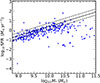 |
Fig. 1. Present-day SFRs against stellar mass for the DustPedia galaxy sample. The solid black line represents the MS of galaxies as defined by Elbaz et al. (2011), while the dashed black lines indicate the 1σ deviations from this sequence. Most of the galaxies lie along the MS, with only a few falling below it. |
To produce the sample of the simulated galaxy spectra, we used the SFHs (derived from real galaxies used in the DestPedia project) as the backbone of this process. For each SFH we produced 1000 mock spectra by drawing each of the other five SPS parameters described earlier from the probability distribution functions described in Table 1 and presented in Fig. 2. This way each simulated spectrum was characterized by an SFH and a vector of SPS parameters drawn from observation-driven distributions. The SFH adopted here comprises two distinct stellar components: a young stellar population and an old stellar population (Ciesla et al. 2016, 2017). These two populations are roughly indicative of a burst or quench of star formation, as well as a more passively evolving stellar component (Nersesian et al. 2019). For the attenuation law, we assumed a starburst curve, as proposed by Calzetti et al. (2000) with a power-law modification introduced by Leitherer et al. (2002). It is important to emphasize that each set of parameters was drawn randomly and independently (not from their joint 5D space), since there are no systematic studies presenting the joint distributions of all these parameters; this is the only available avenue to avoid any biases.
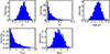 |
Fig. 2. Histograms indicating the shapes and ranges of the distributions of the SPS parameters (Table 1) used as input to the FSPS to produce our mock sample of galaxies. In the top row, from left to right, we show the distribution densities of metallicity (Z), the dust fraction exposed to a high ionization field (γ), and the ionization parameter of the gas (log10U), respectively. On the bottom row on the left, we show the minimum (average) ionization field of the ISM (Umin), while on the bottom right we see the fraction of dust in the form of PAH molecules (qPAH). Each parameter set contains these five parameters drawn randomly and independently from each other based on the probability distributions shown above. |
Our spectra were generated by assuming an SFH each time and varying five parameters, three regarding the dust (i.e., γ, Umin, and qPAH) and two the stellar populations (metallicity and ionization parameter). To assess the variability within the mid-IR spectrum that each dust parameter has, simulated spectra were generated, wherein each dust parameter was allowed to fluctuate within the 95% of its specified probability function (Table 1), while the other dust parameters were drawn from their probability distribution functions as presented in Table 1. It is evident that the three parameters associated with dust models-qPAH, γ, and Umin-have a more significant influence on the mid-IR spectrum (Fig. B.1) than the ones related to stellar (stellar metallicity) and gas (ionization parameter) (Fig. B.2). For more details about the specifics of this exercise, please refer to Appendix B.
2.3. Photometric properties of the simulated galaxy sample
To ensure that our simulated sample accurately reflects the photometric properties of an observed one, we constructed and analyzed color–color diagrams of NUV − r against g − r, g − r against u − g, and W1 − W2 against W2 − W3. By plotting these diagrams, we can visually assess the similarities and discrepancies between the simulated data and the actual observations. This process is crucial for validating the fidelity of our simulations in replicating the observed characteristics of galaxies.
We utilized the NUV photometric band from the Galaxy Evolution Explorer (GALEX; Martin et al. 2005), optical photometry in the u, g, and r bands from the Sloan Digital Sky Survey (SDSS), and the mid-IR W1, W2, and W3 bands from the WISE survey. In order to perform a more thorough comparison between our simulated SED sample and the overall galaxy population, we used for the optical photometry the SDSS (MPA-JHU; Kauffmann et al. 2003; Brinchmann et al. 2004; Tremonti et al. 2004) catalog. We then cross-matched this catalog with the WISE All-sky catalog and the GALEX-SDSS-WISE Legacy Catalog (GSWLC; Salim et al. 2016) to acquire WISE and GALEX photometry, respectively. In order to select star-forming galaxies from this galaxy sample, we used the diagnostic developed by Stampoulis et al. (2019). This diagnostic is based on the joint distribution of the four emission-line ratios: log10([O III]/Hβ), log10([N II]/Hα), log10([S II]/Hα), and log10([O I]/Hα). To ensure reliable classification with the Stampoulis et al. (2019) diagnostic, we imposed a strict selection criterion (S/N > 5 in all emission lines) even for weak emission lines such as the [O I] 6300 Å. This limited the selected population of the star-forming galaxies to the upper limit of the MS (i.e., intense star formation activity). In order to include in our comparison less actively star-forming galaxies that have weaker emission lines, or even galaxies without star-forming activity (passive galaxies), we performed photometric selection also based on the MPA-JHU sample and using the NUV − r versus Mr color magnitude diagram (Haines et al. 2008). Subsequently, we calculated the NUV − r, u − g, g − r, W1 − W2, and W2 − W3 for our mock galaxy sample using the photometry derived from the simulated SEDs.
Figure 3 presents the NUV − r against g − r color–color diagram for the simulated sample (black points) and the observed SDSS sample (red contours) of star-forming and passive galaxies (green contours). In that plot, our sample of simulated galaxies shows good overlap with the sample of the real galaxies in terms of color ranges and distribution, with only a slight deviation for bluer (g − r) colors and slightly redder (NUV − r) colors. Our simulated sample covers smoothly the transition from the bluer star-forming to the redder passive galaxies. However, we see the mock sample of galaxies does not cover the entire distribution of the observed passive galaxies. This is also expected behavior as at the redder end of the NUV − r against g − r color–color plot we have completely inactive galaxies with no star-formation processes, placing them outside the MS.
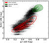 |
Fig. 3. Color–color diagram of NUV − r against g − r comparing the distributions of the mock (black dots) and a real SDSS (red contours) galaxy sample. We see general agreement between the two galaxy samples for almost the entire range of these colors especially for (g − r) ∼ 0.6. Photometric bands from GALEX (NUV) and the SDSS survey (g and r). We also show a sample of photometrically selected passive galaxies (green contours) for comparison. The mock data were artificially augmented with noise to achieve an S/N of 10 to match to the selection criteria for the SDSS and GALEX bands. Contour levels denote the 10th, 25th, 50th, 75th, and 90th percentiles for each population. |
We see similar behavior in the color-color diagram of (g − r) against (u − g), which is shown in Fig. 4. The mock sample follows well the distribution of the SDSS galaxies with the only differences being the slightly redder (u − g) and bluer (g − r) colors, and a lack of the reddest and most passive galaxies. The difference in the bluest and/or UV colors could be the result of differences in the extinction law assumed in the simulations and the actual attenuation curve in real galaxies, which can exhibit diversity from galaxy to galaxy (Salim & Narayanan 2020). Furthermore, this discrepancy may be attributed to the limitations of the emission line grids employed in SED frameworks, which typically only consider emission lines from very young stars (≲10 Myr). This restriction significantly impacts the Hα emission and thus the r-band SDSS magnitudes. The colors we examined above are related to the stellar populations of a galaxy. To ensure that our mock sample of galaxies had dust emission properties similar to that of real galaxies, we also compared their infrared colors. In Fig. 5, we plot the W1 − W2, versus the W2 − W3 colors calculated from the first three WISE bands. In the plot, we observe that the mock galaxies occupy the same range as the SDSS star-forming counterparts for both WISE colors. We also observe similar behavior for the passive galaxies. However, as in Figs. 3 and 4, our mock galaxies do not cover the extreme end of the passive galaxies as expected.
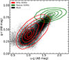 |
Fig. 4. Color–color diagram of g − r against u − g comparing the distributions of a mock (black dots) and a real SDSS (red contours) galaxy sample. We see very good agreement between the two galaxy samples. Photometric bands from the SDSS survey are shown. We also show a sample of photometrically selected passive galaxies (green contours) for comparison. The mock data were artificially augmented with noise to achieve an S/N of 10 to match to the selection criteria for the SDSS bands. Contour levels denote the 10th, 25th, 50th, 75th, and 90th percentiles for each population. |
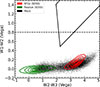 |
Fig. 5. Color–color diagram of W1 − W2 against W2 − W3 comparing the distributions of a mock (black dots) and a real star-forming galaxies from SDSS (red contours). We see very good agreement between the two galaxy samples. Also, both samples occupy the area well bellow the W1 − W2 = 0.8 (dashed black line) demarcation line defined by Stern et al. (2012) between the AGN and non-AGN galaxies and the AGN selection wedge (solid black lines) defined by Mateos et al. (2012). We also show a sample of photometrically selected passive galaxies (green contours) for comparison. Photometric bands from the WISE survey are shown. The mock data were artificially augmented with noise to achieve an S/N of 10 to match to the selection criteria for the WISE bands. Contour levels denote the 10th, 25th, 50th, 75th, and 90th percentiles for each population. |
All the results suggest that the mock SEDs generally have very good agreement with the observed UV to mid-IR SEDs of galaxies. Additionally, the near and mid-IR emission in the mock sample of galaxies are in reasonable agreement with thesimulations.
3. The diagnostic tool
3.1. Identifying the discriminating features
Galaxies’ mid-IR spectra are rich with dust features and atomic lines that are directly linked to the underlying mechanisms heating the dust and gas. For example, the presence of high-ionization lines such as the [Ne V] 14.3 μm and [O IV] 25.9 μm (ionization potential of 97.1 eV and 54.9 eV, respectively) is commonly regarded as a telltale sign of an AGN. However, these features require high-resolution spectra, which can be expensive to acquire, and sometimes also suffer from an additional complication in that their measurement involves subtracting the adjacent MIR continuum, especially in the presence of a bright AGN, or when the galaxy is unresolved. Another disadvantage is that to measure emission-line fluxes one must perform subtraction of the underlying continuum emission (i.e., stellar light and dust emission). This can often be a daunting task as the complex shape of the mid-IR part of the spectrum makes the estimation of the dust emission (i.e., PAHs) and absorption (e.g., silicates) features, very difficult. Even estimating the overall blackbody continuum can be complicated by these broad band features if longer wavelength photometry is not available.
In order to facilitate the analysis of a large volume of data, we focused on spectral bands encompassing diagnostically important features. We took care to avoid including multiple spectral features in each band in order to maximize their diagnostics power.
We did not opt to use photometric filters from existing observatories such as Spitzer, WISE, or JWST because their broadband nature limits their ability to target specific PAH features. Although JWST includes three filters with central wavelengths and bandwidths comparable to our custom bands (i.e., F560W, F770W, and F1130W), its ∼21 μm filter (F2100W) is too broad. It captures not only the underlying dust continuum but also blends PAH emission present in the 15–20 μm, making it unsuitable for isolating the warm continuum emission.
Motivated by the previous studies mentioned above, we began by incorporating features sensitive to the hardness of the radiation (i.e., [Ne V] 14.3 μm and [O IV] 25.9 μm) by defining bands centered on them. However, the underlying continuum proved to be strong enough to dilute any contribution from these emission lines, even in galaxies hosting an AGN. Since our goal was to avoid modeling and removing the continuum, we focused on stronger spectral features that are associated with dust emission (i.e., PAHs). Specifically, we defined three bands to include emission from PAHs targeting the peak wavelengths of 6.2, 7.7 and 8.6, and 11.3 μm. The 12.7 μm PAH feature was excluded from our selected feature scheme due to the substantial contribution from [Ne II] 12.8 μm, which significantly affects that spectral region. Additionally, we designated a band within a featureless (i.e., only continuum emission) part of the spectrum as a proxy for dust temperature and overall normalization. Centered at 21.5 μm, this band serves as an indicator of the warm dust conditions, which is stronger in AGNs, and almost absent in passive galaxies. Table 2 presents all the bands we defined, the wavelength coverage of each custom band, and the PAH features each one includes. We utilized three spectral bands (PAH1, PAH2, and PAH3) containing the PAH features normalized by the continuum band (Cont215) as our discriminating features. After some experimentation, we chose to use the logarithm of these ratios to compress the data ranges and enhance the contribution of features with a small dynamic range.
Wavelength range (rest frame) and important features that describe our custom fixed photometric bands.
We chose the PAH features centered at 6.2, 7.7, 8.6, and 11.3 μm as the basis of our feature scheme because there is no contamination from atomic spectral lines. Another advantage is their proximity to each other making them convenient to observe as they require only a short spectral range making this diagnostic widely applicable to a large number of galaxy samples from retired (e.g., Spitzer) to state-of-the-art (JWST) IR observing facilities. Figure 6 shows an example spectrum of a star-forming galaxy (NGC 6120) observed with the IRS spectrograph. Figure 6 demonstrates how the four fixed custom photometric bands we constructed (Table 2) capture key spectral features characteristic of galaxy activity. In this plot, we see the location of the four custom photometric bands we chose to capture key spectral features that are characteristic of the activity of a galaxy.
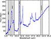 |
Fig. 6. Mid-infrared (5–25 μm) spectrum of NGC 6120, observed with the IRS spectrograph aboard Spitzer, representing a typical star-forming galaxy (BPT class). In this spectrum, we mark the wavelength coverage of our four custom photometric bands, labeled in Table 2. The first three photometric bands (PAH1, PAH2, and PAH3) cover the strongest PAH emission features, while the last band (Cont215) covers a continuum region of the spectrum. |
Having established the diagnostic bands and feature scheme, we proceeded to measure the integrated fluxes within each band and divided the PAH by the continuum band. Figure 7 shows the distributions of PAH1, PAH2, and PAH3 normalized by the continuum at 21–22 μm for the simulated spectral library. In order to verify that our simulated galaxy sample shares the same properties with the observed sample of real galaxies (Sect. 2.1), we compared these distributions between observed and mock galaxies. The distributions are very similar. To quantify this observation, we performed a Kolmogorov–Smirnov (K–S) test on the distribution of each discriminating feature and found the null hypothesis: the observed and mock distributions that come from the same parent distribution cannot be rejected at a significance level higher than ∼15% (p-value ∼ 0.85) for all three features.
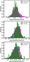 |
Fig. 7. Distributions of the three distinguishing features used to develop our diagnostic tool. From top to bottom: log10(PAH1/Cont215), log10(PAH2/Cont215), and log10(PAH3/Cont215), measured from both the S5 sample (green) of star-forming galaxies and our simulated sample of galaxies (purple). We find very good agreement between the two samples for all the features. |
3.2. Choosing the algorithm
There are several machine learning algorithms that can be applied in classification problems. Since our study is focused on the identification of a single type (class) of objects, i.e., that of populations of star-forming galaxies, it is essential to utilize an algorithm capable of handling single-population data. In general, this type of problem is handled by training an algorithm to learn the characteristics of a population in the selected feature space. After the training, during the classification process, any object that does not belong to the target population is flagged as an outlier. There is a wide variety of such algorithms ranging from more sophisticated (e.g., artificial neural networks) to simpler ones (e.g., isolation forest; Liu et al. 2008). After testing various algorithms, we found that the best performance was achieved by using a variant of the Support Vector Machine (SVM; Cortes & Vapnik 1995), specifically the one-class SVM (OneclassSVM), which is provided through the scikit-learn library based on the Python programming language.
3.3. Training of the algorithm
During training, an SVM aims to find an optimal hyperplane that effectively separates the data points belonging to different classes in a high-dimensional feature space by adjusting the parameters of the hyperplane, guided by the labeled training data (i.e., supervised learning). In our case, the data describe only one galaxy population (star-forming galaxies). The OneClassSVM is an unsupervised algorithm that constructs an envelope around the data based on their distributions in the multidimensional feature space.
As mentioned in Sect. 2.2 the spectra available for training our diagnostic were scarce. For this reason, the training of our diagnostic was conducted exclusively on simulated data, utilizing the library of simulated SEDs introduced in Sect. 2.2. This approach enabled us to employ a large, representative sample of star-forming galaxies in the local Universe overcoming the limitations imposed by the limiting number of observed galaxies. We divided the simulated galaxy sample (Sect. 2.2) into two subsets: 70% for model training and 30% for performance testing.
Following the training phase, we evaluated the diagnostic’s performance on the two simulated test set (which was not involved in the training) and a real galaxy sample (Sect. 2.1). This dual evaluation serves two purposes. First, it allows us to verify that performance for the training and test sets are consistent; discrepancies here could indicate overfitting or underfitting. Second, it allows us to assess diagnostic effectiveness on real (observed) spectra to confirm its applicability and robustness in realistic conditions, ensuring its reliability on observed galaxy data.
4. Results
4.1. Performance metrics
To assess the efficacy of our diagnostic, we began by defining the classification objective: distinguishing between MS star-forming and other types of galaxies (including AGNs, passive galaxies, or even extreme star-forming galaxies such as ULIRGs or metal poor starbursts). We employed widely adopted metrics from supervised learning to quantify performance. Accuracy denotes the proportion of correctly classified galaxies out of the total sample, providing a comprehensive measure of the model’s effectiveness. A high accuracy indicates the correctness of the majority of classifications. Recall, conversely, quantifies the completeness of the identified class, in our context, the fraction of true star-forming galaxies that the model successfully identifies as such. A high recall score signifies the model’s ability to recover the entire target star-forming galaxy population, even if some misclassifications occur. Furthermore, we quantified the contamination from other classes, by recording the number of galaxies that were predicted to be MS star-forming galaxies by our diagnostic but were originally classified (ground truth) to belong to other activity classes (e.g., AGN and composite). Low contamination indicates a highly effective diagnostictool.
4.2. Evaluation of performance
After training and optimizing our diagnostic (see Appendix A for details), we evaluated its performance in two cases. First, we assessed its performance on the test set (see Sect. 3.3) and found it achieves 90% recall, similar to its training set score, ensuring good generalization to similar datasets. When a diagnostic is designed to identify a single class, this evaluation primarily ensures good generalization to other datasets, preventing overfitting. However, it cannot provide information about misclassified objects that do not belong to the targeted class (i.e., contamination, see Appendix A). For the second test, we assessed its performance on an observed sample of star-forming galaxies (Sect. 2.1). This test is essential to validate its relevance for real-world galaxy samples. Achieving a high recall score would not only demonstrate its effectiveness in identifying MS star-forming galaxies but also affirm its reliability for actual observations.
We selected two spectral samples of observed galaxies in order to test the performance of our diagnostic as a function of activity type (see Sect. 3.1). The measurements of the diagnostic features on the observed spectra were performed using the same photometric bands presented in Sect. 2. The activity classification (i.e., the ground truth) of both samples is based on optical spectroscopy (BPT). The first contains MS star-forming galaxies in the local Universe. The application of our diagnostic on that sample should indicate how well it can identify the population of galaxies we are targeting. The other sample contains galaxies that host an active nucleus. The AGN galaxies have generally weaker PAH and stronger mid-IR continuum than star-forming galaxies. Thus, our diagnostic should identify any galaxy that is not related with star formation processes as an abnormal instance and not as normal star-forming galaxy.
After applying our diagnostic to the two samples of observed galaxies (star-forming and AGN), we achieve an overall accuracy of 88.7%. Furthermore, we find that the recall score on the MS star-forming galaxies is 90.9%. In addition, by applying our diagnostic on the sample of spectroscopically identified AGN galaxies we find that 16.2% of AGNs have been classified as normal star-forming galaxies. Overall, the performance of our diagnostic is very high, and similar to the recall we achieved when we evaluated our diagnostic on the mock sample of galaxies. This indicates that our diagnostic can be reliably applied to real galaxies without loss in performance. In addition, the low contamination from AGNs means that the boundaries that contain the star-forming galaxies in the selected feature space are well-defined, offering high recall and low contamination. In Sect. 5.3 we conduct a more thorough analysis of the AGN population that contaminates our diagnostic results.
4.3. Stability of the performance
In order to simulate the effect of different spectral quality, we measured the flux in each of the four custom photometric bands for the star-forming and AGN galaxies in the observed sample. Then, we calculated the values of the discriminating features. For each feature, we draw 1000 samples from a normal distribution. The mean of the distribution is the feature value, and the standard deviation is determined by the target S/N value. We considered data with S/N of 3, 5, 10, and 50. We applied our diagnostic on the sample of real AGN and star-forming galaxies individually, and we recorded the recall of each activity class. for S/N values of 3, 5, 10, and 50. Our results demonstrate that the diagnostic performance is unaffected for both AGN and star-forming galaxies as the recall and the accuracy remained almost unchanged.
These results demonstrate the effectiveness and the robustness of our diagnostic tool in accurately identifying star-forming galaxies even when the measurements are of low quality. In particular, our tool is able to accurately identify MS star-forming galaxies and discriminate them from AGNs with high recall and low contamination.
5. Discussion
In this work, we produced a library of simulated SEDs for MS star-forming galaxies in the local Universe. The sample is representative in terms of covering a wide range of ISM physical parameters (e.g., the dust fraction exposed to a high ionization field, the ionization parameter, the average ionization filed of the ISM, and the fraction of dust in the from of PAH molecules) and stellar populations (SFH and metallicity). Based on this library, we defined a diagnostic tool in order to discern star-forming galaxies from the rest of the galaxy activity types. In the following sections, we discuss into its behavior and its potential limitations.
5.1. PAH emission features as galaxy activity probes
In Sect. 4, we found that our diagnostic achieved excellent performance, even though it was provided with only three discriminating features. This follows from the well known sensitivity of PAHs of the interstellar radiation field and the PAH abundance as a result of star formation (Smith et al. 2007).
It has been observed that AGN-dominated galaxies typically exhibit suppressed PAH emission features, resulting in lower PAH EWs (Armus et al. 2007) compared to star-forming galaxies. This suppression can be attributed to either the destruction of PAH molecules, which are sensitive to radiation strength (Roche et al. 1991; Voit 1992; Siebenmorgen et al. 2004; García-Bernete et al. 2022), or the dilution of their emission in the strong AGN continuum (Alonso-Herrero et al. 2014; Ramos Almeida et al. 2014; García-Bernete et al. 2015).
However, even in galaxies with extreme conditions (i.e., starbursts or AGNs) where the PAH emission is normally expected to be severally depressed, PAH emission can still be detected. In other words, if we rely solely on the presence or the absolute luminosity of PAH features, we may misidentify the activity of these galaxies as that of MS star-forming galaxies. To overcome this limitation, we incorporated an additional band (Cont215, see Table 2) as a normalization factor to enhance the discriminatory power of our diagnostic. This band is sensitive to the hardness of the radiation field that illuminates the dust. As the radiation field becomes harder, the slope at 21–22 μm increases due to the stochastically heated dust or obscuration affecting the continuum emission. Consequently, as the radiation strength of the field increases, we observe a decrease in PAH emission while simultaneously observing an increase in continuum emission at 21–22 μm. This way we can exclude galaxies that may have ongoing star formation under abnormal conditions (i.e., ULIRGs or low-luminosity AGNs) reducing the contamination of non-MS star-forming galaxies in our diagnostic.
5.2. Application on a sample of composite galaxies
In some cases, the activity of a galaxy cannot be uniquely attributed only to star-formation processes or an active nucleus. In other words, a galaxy’s SED may contain contributions by star-formation processes and the presence of an active nucleus. One notable example is the composite galaxies. Naturally, we expect these galaxies to be the transition between pure star-forming galaxies and AGNs. Thus, we wished to test our diagnostic on a sample of composite galaxies in order to assess its performance on galaxies with AGN and star-forming contributions. To do this we identified objects from the SSGSS/S5 survey that have been classified as composites based on their BPT classifications. Then we applied our diagnostic on these samples of galaxies to classify them. We find that 50% are classified as star-forming while the other 50% as not star-forming galaxies.
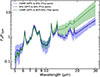 |
Fig. 8. Average mid-IR spectra of composite galaxies (based on the BPT optical diagnostics) classified as star-forming (SFG) and non-star-forming (NOT-SFG) based on our diagnostic. The composite galaxies predicted as star-forming galaxies (solid blue line) have similar average spectra with the typical MS star-forming galaxies (dashed black line). The composite galaxies predicted as not star-forming (solid blue line) have steeper spectra above 12 μm. The shaded area in both average spectra corresponds to the standard deviation of 1σ. |
Afterward, in order to understand the driver of these results, we calculated the average mid-IR spectrum of the galaxies that are classified as star-forming and non-star-forming based on our diagnostic. The average mid-IR spectra were calculated by stacking the individual (rest-frame) mid-IR spectrum for each class after normalizing them at 7 μm. Figure 8 shows the average mid-IR spectrum of composite galaxies (BPT classification) predicted to be star-forming and those predicted as not star-forming (by our diagnostic). It is clear that in the spectral range of 5-13 μm the PAH features are prominent in the two subpopulations making them almost indistinguishable. On the other hand, the average mid-IR spectrum of the composite galaxies that have been predicted as star-forming have significantly lower fluxes in the spectral range above 13 μm. This result indicates that the composite galaxies that have been classified as not resembling a normal star-forming galaxy have dust stronger hot dust emission.
Furthermore, after placing these optically classified composite galaxies on the BPT diagram of [O III]/Hβ versus [N II]/Hα, we do not observed any trend for the composite galaxies that our diagnostic identified as star-forming and for the ones identified as non-star-forming galaxies. All of these observations can be attributed to the fact that dust may hinder our ability to identify an obscured AGN in the optical due to extinction, as suggested by Goulding & Alexander (2009), Hickox & Alexander (2018).
5.3. Physical constraints
In Sect. 4.2 we tested the performance of our diagnostic on a sample of MS star-forming galaxies. However, star formation is also present in galaxies that are away from the MS. For example, ULIRGs have total IR luminosities exceeding 1011 L⊙ and are often associated with ongoing galaxy mergers or interactions, which can trigger intense star-formation (starburst galaxies) or supply material to the nuclear supermassive black hole of the merging galaxies leading to the formation of an AGN.
To assess the performance of our diagnostic in such extreme galaxies, we applied it to galaxies from the GOALS sample. GOALS (Armus et al. 2009) includes 189 nearby galaxies with redshifts ranging from 0.003 to 0.09. Only three galaxies were classified as main-sequence star-forming galaxies by our diagnostic, consistent with our expectations since almost none of them belong to the MS.
The other extreme end in galaxy populations that can harbor star formation are the BCDs. These extremely small-sized galaxies have stellar masses of 107 − 109 M⊙ and typically have high specific star-formation rates (sSFR). To assess the behavior of our diagnostic on that extreme type of galaxies, we used the sample of BCDs of Xie & Ho (2019). We find that none of the BCDs was classified as MS star-forming galaxies according to our diagnostic. This is driven by two effects. The first is that BCDs have suppressed PAH emission (Peeters et al. 2004; Engelbracht et al. 2005; Madden et al. 2006; Wu et al. 2006; Shipley et al. 2016) in their IR spectra. This could be a result of the low metallicities of BCDs leading to low dust content (Draine et al. 2007). The second is that the intense star formation in combination with their low metallicities create a strong UV radiation field, which in combination with the low optical depth of the dust results to stochastic heating of the small dust grains contributing to the mid-IR part of the spectrum (Takeuchi et al. 2003).
In Sect. 4.2 while testing the performance of our diagnostic, we found that 16.2% of the AGN sample (based on optical spectral classifications) were classified as star-forming based on our diagnostic. To analyze this further, we calculated the average spectra of the AGN galaxies (true class) that are classified as star-forming and non star-forming based on our diagnostic. As in the case of the composite galaxies, the spectra are normalized at 7 μm.
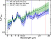 |
Fig. 9. Average mid-IR spectra of AGN galaxies (based on the BPT optical diagnostics) classified as star-forming (SFG) and non-star-forming (NOT-SFG) based on our diagnostic. The AGN galaxies predicted as star-forming galaxies (solid blue line) have similar average spectra with the normal star-forming galaxies (dashed black line). The AGN galaxies that have been predicted as not star-forming (solid blue line) have steeper spectra above 12 μm than the BPT-AGN predicted as star-forming galaxies. In addition, the average spectra of the AGN galaxies identified as non-star-forming exhibit clear emission lines of [Ne V] 14.3 μm (vertical dashed blue line) and [O IV] 25.9 μm (vertical dashed red line). These are tell-tale signs of a strong radiation field source. The shaded area in both average spectra corresponds to the standard deviation of 1σ. |
In Fig. 9 we show these average spectra. The galaxies hosting AGN classified as star-forming have flatter spectra above 14 μm than those classified as non star-forming. In addition, the latter show reduced PAH emission. In the same figure, the average spectra of the AGN misclassified as star-forming resembles that of a typical MS star-forming galaxy. Finally, the AGNs predicted as non-star-forming galaxies show prominent emission from forbidden lines with high ionization potential, such as [Ne V] 14.3 μm and [O IV] 25.9 μm, which are generally absent from the AGNs we classify as star forming.
We further analyze these optically classified galaxies using infrared AGN emission-line diagnostics. One such diagnostic employs the ratio of [O IV] 25.9 μm to the [Ne II] 12.8 μm as a measure of the fractional AGN contribution to the overall galaxy emission (Sturm et al. 2002). Similarly, the EW of the 6.2 μm PAH feature serves as a proxy for the fractional starburst contribution to the galaxy’s luminosity (Armus et al. 2007). Figure 10 shows the [O IV]/[Ne II] ratio as a function of 6.2 μm PAH EW for the same sample of galaxies presented in Figs. 9 and 8. Red circles mark all galaxies that our diagnostic identifies as star-forming. All galaxies classified as star-forming exhibit low AGN fractional contribution to their luminosity (≲10%), as determined by the [O IV]/[Ne II] ratio while they also show high starburst fractional contribution (∼100%), as indicated by the EW of the 6.2 μm PAH feature. Furthermore, it is evident that all AGN and composite galaxies that have been misclassified as star-forming have lower AGN fractional contributions based on the [O IV]/[Ne II] ratio (≲25%) compared to the rest of the AGNs that were identified correctly as non star-forming, while at the same time showing prominent PAH emission based on the EW 6.2 μm PAH feature showing significant starburst fractional contribution (≳50%). This result ensures that our diagnostic is capable of identifying galaxies that their emission is dominated by star formation processes.
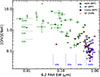 |
Fig. 10. The [O IV] 25.9 μm/[Ne II] 12.8 μm ratio plotted against the EW of the 6.2 μm PAH feature for optically identified star-forming (blue stars), composite (black disks), and AGN (green squares) galaxies. The green lines represent the average AGN fractional contribution to a galaxy’s emission, based on the [O IV]/[Ne II] ratio (Sturm et al. 2002). The blue lines denote the average starburst fractional contribution determined from the EW of the 6.2 μm feature (Armus et al. 2007). The red circle highlights galaxies identified as star-forming based on our diagnostic tool. The uncertainties associated with each measurement are 1σ error. |
5.4. Uncertainties and limitations of dust models
The data used to train our diagnostic in this work are based on synthetic spectra constructed from the Draine et al. (2007) PAH emission templates, which represent a wide variety of dust conditions based on a simplified framework for modeling PAH features in galaxies. While this framework is applicable to typical star-forming galaxies, it may not be applicable to more extreme environments (e.g., starburst and/or low-metallicity galaxies) or in environments with complex activity (e.g., composite galaxies with a weak AGN contribution). These models assume a fixed set of PAH templates and parameterizations (e.g., grain sizedistribution, ionization fraction) and do not fully capture the environmental dependence (e.g., hardness of the starlight ionization field and PAH excitation in a self-consistently way) or intrinsic variability of PAH spectral shapes. Consequently, the learned representations may underperform in environments where PAH emission deviates significantly from the training set (e.g., low-metallicity systems). Future incorporation of more physically detailed models (e.g., Draine et al. 2021) will likely improve both the fidelity and robustness of the predicted spectra. Nevertheless, given that our simulations are confined to MS star-forming galaxies, we anticipate that the measured PAH features from these simulations will not exhibit substantial deviations from spectra obtained from actual galaxies, as demonstrated by the good agreement between the model SEDs and observations of typical star-forming galaxies (e.g., Noll et al. 2009).
5.5. Redshift application range
The use of broadband features (i.e., photometry) can be robust to small changes in distances without requiring redshift corrections because the bands cover a broad area of the spectrum. Here, we investigated how the recall score of the star-forming galaxies would vary as a function of redshift. To accomplish this we applied our trained diagnostic on the simulated sample of galaxies (test set, see Sect. 2.2) by shifting their spectra to increasingly higher redshifts of z = 0, 0.0125, 0.025, 0.05, 0.075, and 0.1. To evaluate the performance, we kept the photometric bands fixed (as defined in Sect. 3.1), and we measured the corresponding flux of each feature in the redshifted spectrum. Figure 11 presents the recall of star-forming galaxies as a function of redshift. As indicated, our recall is high for redshifts up to z ∼ 0.02 and falls linearly for z > 0.02. We chose not to test the performance of our diagnostic beyond z = 0.1 as the edge of our bluer custom band starts to leave the observing window of most infrared observatories.
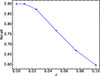 |
Fig. 11. Recall score of our diagnostic as a function of redshift. The performance was recorded by training the algorithm using rest-frame spectra and testing the performance on the test sample of the redshifted simulated spectra at z= 0, 0.0125, 0.025, 0.05, 0.075, and 0.1. The scores are stable for up to z ∼ 0.02 and then drop smoothly. |
5.6. Applicability limits
Our diagnostic tool was developed to identify MS star-forming galaxies, which are distinct from other types of galaxies that host star formation, such as starburst galaxies ULIRGs and BCDs. The MS galaxies have different infrared properties (e.g., colors) when compared to other extreme classes of star-forming galaxies, such as BCDs or ULIRGs, as the latter two both have red IR colors (Hainline et al. 2016). In this section we aim to assess the applicability of our diagnostic on different samples of galaxies as defined by their IR properties (e.g., colors and magnitudes) by identifying areas on color-color and magnitude-magnitude diagrams.
We sought the locus within the MS where our diagnostic correctly identified star-forming galaxies, in order to identify the limits within which it worked optimally. For that reason, the samples of GOALS, ULIRGs, BCDs, and S5 were cross-matched with the WISE All-sky catalog to acquire their W4 magnitudes, and utilizing the SFR-W4 SFR calibration of Cluver et al. (2017), we calculated the SFRs of all galaxies. The left panel of Fig. 12 shows our results from the application of our diagnostic to the aforementioned samples of galaxies on the SFR-stellar mass plot. We adopt the MS definition from Elbaz et al. (2011). In that figure, BCDs and ULIRGs deviate from the best-fit line that contains normal SF galaxies.
However, stellar mass and SFR estimations can sometimes be difficult to acquire. For this reason, we also considered infrared photometric bands from all-sky surveys as these include a large number of galaxies making it easily applicable for large datasets. Thus, we used the four WISE bands (W1, W2, W3, and W4) to calculate the absolute magnitudes of W1 and W4. In Fig. 12 (right panel), we plot the W4 absolute magnitude against the W1 absolute magnitude. The former provides an approximation of the star-formation rate of a star-forming galaxy (Cluver et al. 2017), while the latter provides an estimation of the stellar mass.
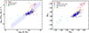 |
Fig. 12. Star formation rate against stellar mass for galaxies from several galaxy samples (left panel). We correctly identify almost all the galaxies that fall in the area on the MS star-forming galaxies. As expected, we miss all the galaxies from samples that focus on BCDs and ULIRGs. The solid blue line shows the MS fit for star-forming galaxies from Elbaz et al. (2011), and the dashed blue lines are correspond to the 1σ error to this line. On the right panel, we plot the absolute magnitude in band W4 against the absolute magnitude in band W1 for the same galaxies. The former serves as a proxy of the star formation rate, while the latter as a proxy of the stellar mass of a galaxy. The star-forming galaxies identified correctly (blue circles) are clustered on the MS, while the star-forming galaxies missed tend to have higher MW4 values or correspond to extreme cases of galaxies (BCDs or ULIRGs). |
Furthermore, a widely used IR color-color plot is the W1 − W2 versus W2 − W3. in Fig. 13, we present the of W1 − W2 versus W2 − W3 color-color plot, utilizing the same sample of galaxies as in in Fig. 12. In Fig. 13, we see that MS star-forming galaxies occupy a specific region on this color-color plot, characterized by bluer W1 − W2 colors than the more extreme star-forming galaxies (BCDs and ULIRGs). This region is bounded by two straight lines of W1 − W2 < 0.3 and W2 − W3 < 3.7. Based on this observation we propose this selection criteria as a test for the applicability of our diagnostic. Additionally, in the same figure, we observe that the MS star-forming galaxies, which our diagnostic failed to identify correctly (9.1% of the MS star-forming galaxies from the S5 sample), have redder W1 − W2 and W2 − W3 colors compared to those correctly identified. Galaxies exhibiting such IR colors can be AGN hosts or extreme starbursts (Hainline et al. 2016; Daoutis et al. 2023).
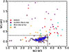 |
Fig. 13. Color–color plot of W1 − W2 against the W2 − W3 for the same samples of galaxies introduced in Fig. 12. The normal star-forming galaxies we have identified correctly occupy the lower area of this plot, while extreme cases related to star formation (such as BCDs and ULIRGs) are scattered, exhibiting redder W1 − W2 and W2 − W3 colors. The dashed black lines delineate the optimal operational area of our diagnostic system. |
5.7. Comparison with other methods
The custom diagnostic bands we defined for this diagnostic (Sect. 3.1) have the advantage of targeting specific spectral features, offering high discriminating power. They also provide unbiased measurements, unlike existing IR diagnostics (e.g., emission lines and 6.2 μm EW) that require continuum subtraction and assumptions about the underlying dust continuum, which can lead to biased EWs by a factor of ∼2–3 (Smith et al. 2007).
In order to compare the performance of our diagnostic with other similar diagnostic methods, we used the diagnostic based on EW of 6.2 μm PAH introduced in Sect. 5.1. Galaxies with an EW below 0.2 μm are classified as AGNs, while those with an EW between 0.2 and 0.5 μm are classified as composite, and those with an EW above 0.5 μm are designated as star-forming galaxies.
Our comparison is based on star-forming galaxies from the S5 sample because they represent a wide range of MS galaxy conditions (see Sect. 2.1). However, this sample lacks galaxies of other activity types, such as composite and AGN galaxies. To address this limitation, we supplemented our sample with composite and AGN galaxies from the IDEOS sample (Sect. 2.1).
Although the IDEOS sample provides various observables for its galaxies, it does not offer activity classifications based on optical methods. Therefore, we cross-matched the IDEOS catalog with the SDSS DR8 to obtain optical emission line fluxes, such as Hα, Hβ, [N II], [O III], and [S II] and determined their activity based on the emission-line ratios of log10([N II]/Hα), log10([S II]/Hα), and log10([O III]/Hβ). To maintain consistency with the real galaxy sample (see Sect. 2.1), these galaxies have to be classified using an optical emission line diagnostic. Thus, we employed the classification tool developed by Stampoulis et al. (2019), which is based on the location of each galaxy in the 3D emission-line ratio space using the aforementioned spectral lines. This approach is advantageous to the traditional 2D diagnostic diagrams as it simultaneously considers three of the strongest optical emission lines avoiding contradictory classifications between the different 2D diagnostics.
To ensure the use of high quality data in this comparison, we filtered the S4 and IDEOS spectra by selecting those with S/N greater than 5 at the 14 μm continuum. In addition we considered, only measurements with S/N greater than 3 for the EW of 6.2 μm PAH feature. For the quality of the optical classifications, we selected galaxies with an S/N greater than 5 in all the emission lines used (i.e., Hα, Hβ, [O III], [N II], and [S II]). Our final comparison sample consists of 138 star-forming galaxies, 127 AGNs, and 108 composite galaxies. We compared our method with the EW6.2 diagnostic and the optical classification, which serves as the ground truth. The results of this comparison are summarized in Table 3.
Comparison of the activity classification between our diagnostic and the 6.2 μm PAH EW classifier (EW6.2).
From these classification results, our diagnostic correctly identifies 90% of the star-forming galaxies, while the EW6.2 method correctly identifies all of them. Closer inspection of the mid-IR SEDs of these misclassified galaxies reveals that they do not share the same properties as typical MS star-forming galaxies since their mid-IR SEDs are similar to the composite galaxies that our diagnostic predicted as as not star-forming galaxies shown in Fig. 8.
For the optically classified AGN galaxies, our diagnostic misclassified only one AGN as a star-forming galaxy, whereas the EW6.2 method misclassified nearly half of them as star-forming. Upon examining the SEDs, we find that the one galaxy our diagnostic misclassified as star-forming has an SED similar to a typical MS star-forming galaxy (see Fig. 9).
When comparing the activity class of composite galaxies, our diagnostic results in classifying 33% of them as star-forming and the other 67% as non-star-forming. In contrast, the EW6.2 method identifies almost all composite galaxies as star-forming, with only one classified as composite and another as AGN. By visually inspecting the SEDs of the composite galaxies classified by our diagnostic, we find that those predicted as star-forming have SEDs consistent with the average spectrum of a typical star-forming galaxy (e.g., they lack PAH emission and have steeper IR continuum), while those predicted as non-star-forming do not exhibit similarities with star-forming galaxies (see Fig. 8 and Sect. 5.2 for a more detailed discussion). This result shows that our diagnostic can identify galaxies that, despite exhibiting high 6.2 μm EW, which is usually linked to star-forming galaxies, they cannot be characterized as MS star-forming galaxies. The presence of the steeper slope indicates more intense ionization fields illuminating the dust than those typically found in normal MS star-forming galaxies.
In conclusion, we observe that the main differentiating factor in all these cases is the continuum emission at 22 μm. This indicates that our diagnostic is sensitive to the stronger dust emission that can be a result of a harder radiation field (i.e., higher temperature dust), even in the presence of significant PAH emission, which in some cases seems to confuse the EW6.2 diagnostic.
5.8. Potential application to JWST/MIRI spectra
Since PAH features are broad spectral features present over a wide spectral range, we expect that our diagnostic will be applicable to spectra acquired with different instruments regardless of their resolving power. JWST, in particular, enables the acquisition of high quality spectra from a much larger population of galaxies than was possible with previous instruments.
In order to verify the applicability of our diagnostic to data obtained with JWST, we applied it to data obtained with the MIRI spectrograph aboard JWST. We used spectra extracted from galaxy cores that are known to host AGNs (NGC 7469) and galaxies that have star forming regions scattered across the disk (VV114). The extraction of the spectra was performed using the Continuum And Feature Extraction (CAFE; Diaz-Santos et al. (2025)4). Then, we measured the intensity of our four diagnostic bands on their rest-frame spectra. We find that all the AGN spectra are correctly identified as not being MS star-forming galaxies, while the spectra extracted from the H II regions are correctly identified as resembling MS star-forming galaxies. This exercise proves that our diagnostic can indeed applied to spectra recorded with different spectral resolution.
5.9. A photometric diagnostic optimized for JWST
As discussed in Sect. 3.1, our custom photometric bands are designed to specifically target specific, physically motivated, PAH and continuum features that have demonstrated exceptional effectiveness in identifying MS star-forming galaxies from their IR spectra. However, photometric observations are generally easier to obtain than spectroscopy, and with JWST’s growing archival database, it is both timely and valuable to develop a diagnostic tailored in identifying MS star-forming galaxies using JWST photometry alone. While previous missions such as WISE and Spitzer (e.g., IRAC and MIPS) have offered broad mid-IR coverage, their wider filter profiles often blend PAH emission features with the underlying continuum, which can dilute the PAH characteristics we aim to isolate. In contrast, JWST’s narrower, more precisely defined filters provide an opportunity to isolate key PAH signatures with greater clarity, improving the reliability of photometric diagnostics. Thus, prompted by the results presented in the previous sections we define an additional diagnostic tool that is tailored to the JWST photometry.
To accomplish this objective, we identified JWST bands that span the 5–24 μm wavelength range form the MIRI instrument. From the diverse available filters, we selected those that resample the wavelength ranges more closely to our photometric band scheme (Table 2). This way we selected the F560W, F770W, F1130W, and F2100W filters. Based on these bands, we calculated the flux ratios of F560W/F2100W, F770W/F2100W, and F1130W/F2100W as discriminating features equivalent to our diagnostic scheme.
Afterward, we trained and evaluated our diagnostic according to the procedures described in Sects. 3.3 and 4.2, respectively. More specifically, we began by calculating the synthetic fluxes on the simulated spectra (Sect. 2.2) by convolving them with the response of each selected JWST filter (filter response curves taken from Spanish Virtual Observatory (SVO)5). After training the new diagnostic, we evaluated its performance on the sample of real galaxies (Sect. 2.1 and Table 3). This sample did not have available JWST photometry. For this reason, we calculated their synthetic fluxes by convolving their Spitzer/IRS spectra as we did for the simulated spectra. In Table 4 we present the results of the application of the JWST-optimized diagnostic on the JWST photometry calculated for the real galaxy sample presented in Table 3.
Classification results for a sample of real galaxies based on the diagnostic tailored for JWST/MIRI photometry.
Based on the results presented in Table 4, we see several notable distinctions between the JWST-optimized tool and the tool described in the previous sections. First, the new diagnostic shows improved performance in identifying MS star-forming galaxies, increasing from 90% to 95%. However, this improvement comes with trade-offs. Of the 127 AGNs in the sample, 35 (28%) are misclassified as MS star-forming galaxies-doubling the AGN contamination rate compared to the previous diagnostic (which was 12.5%). Additionally, the JWST/MIRI filter-based diagnostic classifies the majority of composite galaxies (∼91%) as MS star-forming, contributing further contamination. Figure 8 shows that a substantial subset of our sample of composites (∼67%) exhibit prominent AGN signatures, such as [Ne V] and [O IV] emission lines in their spectra, suggesting that they are not MS star-forming galaxies.
These results indicate that while the JWST diagnostic slightly improves the identification of MS star-forming galaxies, it also increases misclassification of AGNs and composites, limiting its reliability for defining a clean MS star-forming sample. This reinforces the conclusion that our custom-selected bands offer a more optimal feature set for discrimination. The reason why the JWST filters underperform in this context may be that, although the first three filters span similar wavelength range as our scheme, the F2100W filter spans a wider range (17.9–24.5 μm). This prevents it from isolating the warm dust continuum effectively, as it overlaps with PAH features in the 15–20 μm region. Nonetheless, this diagnostic can be used to obtain a baseline sample of MS galaxies from JWST photometric surveys, albeit with the aforementioned limitations.
6. Conclusions
In this work, we developed a diagnostic for MS star-forming galaxies in the local Universe by combining a library of simulated IR spectra and machine learning methods. Our results can be summarized as follows.
-
We built a library of synthetic UV to IR spectra of non-AGN galaxies, by sampling parameters for the stellar populations and ISM obtained from extensive observational studies. We find that the optical and near- and/or mid-IR colors of these simulated spectra are consistent with the observed colors of large galaxy samples. Nevertheless, we observe general agreement between the simulated galaxies’ UV colors and the actual sample. Notably, objects located in the middle of the NUV − r band exhibit a systematic offset.
-
We built a diagnostic tool based on photometric bands centered on dust emission features (PAHs and continuum). This diagnostic can reliably identify MS sequence star-forming galaxies with minimal contamination by AGNs. The use of broadband photometry circumvents the process of estimating and subtracting the underlying continuum; hence, a process can introduce inherent biases.
-
Due to the utilization of broad bands and the fact that PAHs and continuum features employed here are effectively insensitive to the resolution of the spectrograph utilized to record the spectra, our diagnostic can be applied to spectra acquired from other observatories without any modifications, such as JWST.
-
In addition to our diagnostic, we provided a separate diagnostic tool optimized for JWST photometry using only four JWST/MIRI filters: F560W, F770W, F1130W, and F2100W. While the JWST diagnostic exhibits reduced performance compared to our original scheme, it remains highly relevant for future analyses based on JWST data as more data becomes available.
Extensions of this diagnostic include a study of the sensitivity of this diagnostic to the presence of weak AGNs and the characterization of extreme starbursts (e.g., BCDs and ULIRGs).
Data availability
Our diagnostic, including the version tailored for JWST/MIRI photometry, will be made publicly available on GitHub: https://github.com/BabisDaoutis/MSMIRdiagnostic, accompanied by detailed documentation and usage instructions.
Acknowledgments
We would like to express our sincere gratitude to the anonymous referee for their thoughtful comments and constructive suggestions, which have helped improve the clarity and quality of the manuscript. We would like to express our sincere gratitude to Dr. Angelos Nersessian and Dr. Emmanuel Xilouris for results from the dustPedia analysis that are used in our analysis, Dr. Benjamin Johnson for insightful discussions on the SED simulations. C.D. acknowledges support from the Public Investments Program through a Matching Funds grant to the IA-FORTH. The research leading to these results has received funding from the European Research Council under the European Union’s Seventh Framework Programme (FP/2007-2013)/ERC Grant Agreement n. 617001, the European Union’s Horizon 2020 research and innovation programme under the Marie Skłodowska-Curie RISE action, Grant Agreement n.873089 (ASTROSTAT-II), and the Smithsonian Astrophysical Observatory Predoctoral Program with funding under the NASA grant 80NSSC21K0078. This research has made use of the NASA/IPAC Infrared Science Archive, which is funded by the National Aeronautics and Space Administration and operated by the California Institute of Technology. DustPedia is a collaborative focused research project supported by the European Union under the Seventh Framework Programme (2007–2013) call (proposal no. 606847). The participating institutions are: Cardiff University, UK; National Observatory of Athens, Greece; Ghent University, Belgium; Université Paris Sud, France; National Institute for Astrophysics, Italy and CEA, France. Funding for the Sloan Digital Sky Survey IV has been provided by the Alfred P. Sloan Foundation, the U.S. Department of Energy Office of Science, and the Participating Institutions. SDSS-IV acknowledges support and resources from the Center for High Performance Computing at the University of Utah. The SDSS website is www.sdss.org. SDSS-IV is managed by the Astrophysical Research Consortium for the Participating Institutions of the SDSS Collaboration including the Brazilian Participation Group, the Carnegie Institution for Science, Carnegie Mellon University, Center for Astrophysics | Harvard & Smithsonian, the Chilean Participation Group, the French Participation Group, Instituto de Astrofísica de Canarias, The Johns Hopkins University, Kavli Institute for the Physics and Mathematics of the Universe (IPMU) / University of Tokyo, the Korean Participation Group, Lawrence Berkeley National Laboratory, Leibniz Institut für Astrophysik Potsdam (AIP), Max-Planck-Institut für Astronomie (MPIA Heidelberg), Max-Planck-Institut für Astrophysik (MPA Garching), Max-Planck-Institut für Extraterrestrische Physik (MPE), National Astronomical Observatories of China, New Mexico State University, New York University, University of Notre Dame, Observatário Nacional / MCTI, The Ohio State University, Pennsylvania State University, Shanghai Astronomical Observatory, United Kingdom Participation Group, Universidad Nacional Autónoma de México, University of Arizona, University of Colorado Boulder, University of Oxford, University of Portsmouth, University of Utah, University of Virginia, University of Washington, University of Wisconsin, Vanderbilt University, and Yale University.
References
- Allamandola, L. J., Tielens, A. G. G. M., & Barker, J. R. 1985, ApJ, 290, L25 [Google Scholar]
- Alonso-Herrero, A., Ramos Almeida, C., Esquej, P., et al. 2014, MNRAS, 443, 2766 [NASA ADS] [CrossRef] [Google Scholar]
- Aniano, G., Draine, B. T., Hunt, L. K., et al. 2020, ApJ, 889, 150 [NASA ADS] [CrossRef] [Google Scholar]
- Armus, L., Charmandaris, V., Bernard-Salas, J., et al. 2007, ApJ, 656, 148 [NASA ADS] [CrossRef] [Google Scholar]
- Armus, L., Mazzarella, J. M., Evans, A. S., et al. 2009, PASP, 121, 559 [Google Scholar]
- Assef, R. J., Stern, D., Noirot, G., et al. 2018, ApJS, 234, 23 [Google Scholar]
- Baldwin, J. A., Phillips, M. M., & Terlevich, R. 1981, PASP, 93, 5 [Google Scholar]
- Boquien, M., Burgarella, D., Roehlly, Y., et al. 2019, A&A, 622, A103 [NASA ADS] [CrossRef] [EDP Sciences] [Google Scholar]
- Brinchmann, J., Charlot, S., White, S. D. M., et al. 2004, MNRAS, 351, 1151 [Google Scholar]
- Calzetti, D., Armus, L., Bohlin, R. C., et al. 2000, ApJ, 533, 682 [NASA ADS] [CrossRef] [Google Scholar]
- Carnall, A. C., McLure, R. J., Dunlop, J. S., & Davé, R. 2018, MNRAS, 480, 4379 [Google Scholar]
- Chevallard, J., & Charlot, S. 2016, MNRAS, 462, 1415 [NASA ADS] [CrossRef] [Google Scholar]
- Ciesla, L., Boselli, A., Elbaz, D., et al. 2016, A&A, 585, A43 [NASA ADS] [CrossRef] [EDP Sciences] [Google Scholar]
- Ciesla, L., Elbaz, D., & Fensch, J. 2017, A&A, 608, A41 [NASA ADS] [CrossRef] [EDP Sciences] [Google Scholar]
- Cluver, M. E., Jarrett, T. H., Dale, D. A., et al. 2017, ApJ, 850, 68 [Google Scholar]
- Conroy, C., Gunn, J. E., & White, M. 2009, ApJ, 699, 486 [Google Scholar]
- Cortes, C., & Vapnik, V. 1995, Machine learning, 20, 273 [Google Scholar]
- Coziol, R., Torres-Papaqui, J. P., Plauchu-Frayn, I., et al. 2014, Rev. Mex. Astron. Astrofis., 50, 255 [NASA ADS] [Google Scholar]
- Curti, M., Hayden-Pawson, C., Maiolino, R., et al. 2022, MNRAS, 512, 4136 [NASA ADS] [CrossRef] [Google Scholar]
- Daoutis, C., Kyritsis, E., Kouroumpatzakis, K., & Zezas, A. 2023, A&A, 679, A76 [NASA ADS] [CrossRef] [EDP Sciences] [Google Scholar]
- Diaz-Santos, T., Lai, T. S. Y., Finnerty, L., et al. 2025, Astrophysics Source Code Library [record ascl:2501.001] [Google Scholar]
- Draine, B. T., Dale, D. A., Bendo, G., et al. 2007, ApJ, 663, 866 [NASA ADS] [CrossRef] [Google Scholar]
- Draine, B. T., Li, A., Hensley, B. S., et al. 2021, ApJ, 917, 3 [CrossRef] [Google Scholar]
- Elbaz, D., Dickinson, M., Hwang, H. S., et al. 2011, A&A, 533, A119 [NASA ADS] [CrossRef] [EDP Sciences] [Google Scholar]
- Engelbracht, C. W., Gordon, K. D., Rieke, G. H., et al. 2005, ApJ, 628, L29 [NASA ADS] [CrossRef] [Google Scholar]
- Galliano, F., Madden, S. C., Jones, A. P., Wilson, C. D., & Bernard, J. P. 2005, A&A, 434, 867 [CrossRef] [EDP Sciences] [Google Scholar]
- Galliano, F., Nersesian, A., Bianchi, S., et al. 2021, A&A, 649, A18 [EDP Sciences] [Google Scholar]
- García-Bernete, I., Ramos Almeida, C., Acosta-Pulido, J. A., et al. 2015, MNRAS, 449, 1309 [CrossRef] [Google Scholar]
- García-Bernete, I., Rigopoulou, D., Alonso-Herrero, A., et al. 2022, MNRAS, 509, 4256 [Google Scholar]
- Gardner, J. P., Mather, J. C., Clampin, M., et al. 2006, Space Sci. Rev., 123, 485 [Google Scholar]
- Goulding, A. D., & Alexander, D. M. 2009, MNRAS, 398, 1165 [NASA ADS] [CrossRef] [Google Scholar]
- Haines, C. P., Gargiulo, A., & Merluzzi, P. 2008, MNRAS, 385, 1201 [NASA ADS] [CrossRef] [Google Scholar]
- Hainline, K. N., Reines, A. E., Greene, J. E., & Stern, D. 2016, ApJ, 832, 119 [CrossRef] [Google Scholar]
- Hernán-Caballero, A., Spoon, H. W. W., Lebouteiller, V., Rupke, D. S. N., & Barry, D. P. 2016, MNRAS, 455, 1796 [CrossRef] [Google Scholar]
- Hickox, R. C., & Alexander, D. M. 2018, ARA&A, 56, 625 [Google Scholar]
- Ho, L. C., Filippenko, A. V., & Sargent, W. L. W. 1997, ApJS, 112, 315 [NASA ADS] [CrossRef] [Google Scholar]
- Hony, S., Van Kerckhoven, C., Peeters, E., et al. 2001, A&A, 370, 1030 [CrossRef] [EDP Sciences] [Google Scholar]
- Houck, J. R., Roellig, T. L., van Cleve, J., et al. 2004, ApJS, 154, 18 [NASA ADS] [CrossRef] [Google Scholar]
- Jarrett, T. H., Cohen, M., Masci, F., et al. 2011, ApJ, 735, 112 [Google Scholar]
- Johnson, B. D., Leja, J., Conroy, C., & Speagle, J. S. 2021, ApJS, 254, 22 [NASA ADS] [CrossRef] [Google Scholar]
- Kauffmann, G., Heckman, T. M., Tremonti, C., et al. 2003, MNRAS, 346, 1055 [Google Scholar]
- Kennicutt, R. C., Jr, Armus, L., Bendo, G., et al. 2003, PASP, 115, 928 [NASA ADS] [CrossRef] [Google Scholar]
- Kewley, L. J., Dopita, M. A., Sutherland, R. S., Heisler, C. A., & Trevena, J. 2001, ApJ, 556, 121 [Google Scholar]
- Kewley, L. J., Nicholls, D. C., & Sutherland, R. S. 2019, ARA&A, 57, 511 [Google Scholar]
- Kovlakas, K., Zezas, A., Andrews, J. J., et al. 2021, MNRAS, 506, 1896 [NASA ADS] [CrossRef] [Google Scholar]
- Laurent, O., Mirabel, I. F., Charmandaris, V., et al. 2000, A&A, 359, 887 [NASA ADS] [Google Scholar]
- Leger, A., & Puget, J. L. 1984, A&A, 137, L5 [Google Scholar]
- Leitherer, C., Li, I. H., Calzetti, D., & Heckman, T. M. 2002, ApJS, 140, 303 [NASA ADS] [CrossRef] [Google Scholar]
- Liu, F. T., Ting, K. M., & Zhou, Z. H. 2008, 2008 Eighth IEEE International Conference on Data Mining, 413 [Google Scholar]
- Madden, S. C. 2000, New Astron. Rev., 44, 249 [Google Scholar]
- Madden, S. C., Galliano, F., Jones, A. P., & Sauvage, M. 2006, A&A, 446, 877 [NASA ADS] [CrossRef] [EDP Sciences] [Google Scholar]
- Martin, D. C., Fanson, J., Schiminovich, D., et al. 2005, ApJ, 619, L1 [Google Scholar]
- Mateos, S., Alonso-Herrero, A., Carrera, F. J., et al. 2012, MNRAS, 426, 3271 [Google Scholar]
- Nersesian, A., Xilouris, E. M., Bianchi, S., et al. 2019, A&A, 624, A80 [NASA ADS] [CrossRef] [EDP Sciences] [Google Scholar]
- Noll, S., Burgarella, D., Giovannoli, E., et al. 2009, A&A, 507, 1793 [NASA ADS] [CrossRef] [EDP Sciences] [Google Scholar]
- O’Dowd, M. J., Schiminovich, D., Johnson, B. D., et al. 2011, ApJ, 741, 79 [Google Scholar]
- Peeters, E., Spoon, H. W. W., & Tielens, A. G. G. M. 2004, ApJ, 613, 986 [NASA ADS] [CrossRef] [Google Scholar]
- Ramos Almeida, C., Alonso-Herrero, A., Esquej, P., et al. 2014, MNRAS, 445, 1130 [NASA ADS] [CrossRef] [Google Scholar]
- Roche, P. F., Aitken, D. K., Smith, C. H., & Ward, M. J. 1991, MNRAS, 248, 606 [NASA ADS] [CrossRef] [Google Scholar]
- Salim, S., & Narayanan, D. 2020, ARA&A, 58, 529 [NASA ADS] [CrossRef] [Google Scholar]
- Salim, S., Lee, J. C., Janowiecki, S., et al. 2016, ApJS, 227, 2 [NASA ADS] [CrossRef] [Google Scholar]
- Schawinski, K., Thomas, D., Sarzi, M., et al. 2007, MNRAS, 382, 1415 [Google Scholar]
- Schiminovich, D., Charlot, S., da Cunha, E., et al. 2008, S5: The Spitzer SDSS Statistical Spectroscopic Survey, SpitzerProposal ID #50568 [Google Scholar]
- Shipley, H. V., Papovich, C., Rieke, G. H., Brown, M. J. I., & Moustakas, J. 2016, ApJ, 818, 60 [NASA ADS] [CrossRef] [Google Scholar]
- Siebenmorgen, R., Krügel, E., & Spoon, H. W. W. 2004, A&A, 414, 123 [NASA ADS] [CrossRef] [EDP Sciences] [Google Scholar]
- Smith, J. D. T., Dale, D. A., Armus, L., et al. 2004, ApJS, 154, 199 [Google Scholar]
- Smith, J. D. T., Draine, B. T., Dale, D. A., et al. 2007, ApJ, 656, 770 [Google Scholar]
- Spinoglio, L., & Malkan, M. A. 1992, ApJ, 399, 504 [NASA ADS] [CrossRef] [Google Scholar]
- Spoon, H. W. W., Marshall, J. A., Houck, J. R., et al. 2007, ApJ, 654, L49 [Google Scholar]
- Spoon, H. W. W., Hernán-Caballero, A., Rupke, D., et al. 2022, ApJS, 259, 37 [NASA ADS] [CrossRef] [Google Scholar]
- Stampoulis, V., van Dyk, D. A., Kashyap, V. L., & Zezas, A. 2019, MNRAS, 485, 1085 [NASA ADS] [CrossRef] [Google Scholar]
- Stern, D., Assef, R. J., Benford, D. J., et al. 2012, ApJ, 753, 30 [Google Scholar]
- Sturm, E., Lutz, D., Verma, A., et al. 2002, A&A, 393, 821 [NASA ADS] [CrossRef] [EDP Sciences] [Google Scholar]
- Takeuchi, T. T., Hirashita, H., Ishii, T. T., Hunt, L. K., & Ferrara, A. 2003, MNRAS, 343, 839 [CrossRef] [Google Scholar]
- Tielens, A. G. G. M. 2008, ARA&A, 46, 289 [NASA ADS] [CrossRef] [Google Scholar]
- Tremonti, C. A., Heckman, T. M., Kauffmann, G., et al. 2004, ApJ, 613, 898 [Google Scholar]
- Voit, G. M. 1992, MNRAS, 258, 841 [NASA ADS] [CrossRef] [Google Scholar]
- Werner, M. W., Roellig, T. L., Low, F. J., et al. 2004, ApJS, 154, 1 [NASA ADS] [CrossRef] [Google Scholar]
- Whitcomb, C. M., Smith, J. D. T., Sandstrom, K., et al. 2024, ApJ, 974, 20 [Google Scholar]
- Wright, E. L., Eisenhardt, P. R. M., Mainzer, A. K., et al. 2010, AJ, 140, 1868 [Google Scholar]
- Wu, Y., Charmandaris, V., Hao, L., et al. 2006, ApJ, 639, 157 [NASA ADS] [CrossRef] [Google Scholar]
- Xie, Y., & Ho, L. C. 2019, ApJ, 884, 136 [CrossRef] [Google Scholar]
Appendix A: Optimization of significant parameters
As machine learning algorithms often have a lot of parameters that potentially take a number of different values. This makes them highly versatile offering them the ability to adapt to a huge number of datasets. Thus, a crucial step toward defining a new diagnostic tool is to optimize it so that the algorithm could be tailored to fit the individual needs of a problem making it work at its peak performance.
Optimization typically involves selecting parameters that significantly impact the algorithm’s performance. For each parameter, a range of values is chosen, and a grid search explores all possible combinations. This process utilizes cross-validation, a robust technique for evaluating and improving the performance of machine learning models by reducing overfitting and ensuring generalization.
In k-fold cross-validation, the dataset is divided into k equally sized folds. The model is trained on k-1 folds and tested on the remaining fold, with this process repeated k times to ensure each fold serves as the test set once. The results are averaged to provide a comprehensive performance metric. This method offers a better performance estimation compared to a single train-test split and makes full use of the available data, as each data point is included in both training and test sets across iterations.
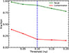 |
Fig. A.1. Recall for star-forming galaxies, indicated by the green line, and contamination from AGNs, indicated by the red line. Both metrics were calculated on the observed sample (Sect. 2.1) as a function of the oneclassSVM nu parameter (i.e., population selection threshold). We observe that contamination begins to increase rapidly after nu = 0.9, marked by a horizontal blue line, which designates our selected value for nu. |
Here, we are dealing with an algorithm designed to recognize only one population of objects. During its training, the oneclassSVM fits a surface in the selected feature space to encompass a user-defined fraction of the whole population. Data inside these boundaries are considered normal cases, while everything outside is considered an outlier. Thus, an assumption is made about what fraction of the given data represents the true population.
We perform the optimization of our diagnostic in two steps. The first step involves identifying the parameters that significantly impact performance. This step has two main purposes: to prevent the algorithm from overfitting the data and to achieve the best performance. After investigation, we found that the parameters with the highest impact on performance are gamma and kernel. Using exclusively the mock sample of galaxies (see Sect. 2.2) and the k-fold cross-validation method, we determined the best values for these parameters, as shown in Table A.1. The remaining parameters are kept at their default values as specified by oneclassSVM.
Parameters of the one-class SVM, their ranges, and best values.
The second step is to find the optimal value for the parameter that sets the fraction of the population representing the instances the diagnostic will identify as normal instances (MS star-forming galaxies).
In oneclassSVM, the parameter nu plays a pivotal role in determining the model’s behavior. Acting as both an upper bound on the fraction of outliers and a lower bound on the fraction of support vectors, the nu parameter allows fine-tuning of the model’s sensitivity to anomalies. By adjusting nu, we can achieve a balance between false positives and false negatives, influencing the model’s classification of data points as normal or outliers.
This parameter, nu, needs to be optimized independently from the others because it is not related to the fitting process but rather to the trade-off between recall and contamination. Specifically, one could choose a boundary that includes all objects in the population (i.e., nu = 0 and recall = 1). However, due to the continuous nature of galaxies, the transition between different activity classes occurs gradually. This means that selecting nu = 0 would result in high contamination, with other activity classes, such as AGNs, being misclassified as star-forming galaxies.
After determining the optimal values of the parameters (all except nu) in the first step of the optimization process, we proceeded to find the optimal value of nu that simultaneously maximizes recall and minimizes contamination. To accomplish this, we utilized the sample of observed galaxies (see Sect. 2.1), aiming to tailor our diagnostic to perform optimally in real-world scenarios. We selected five values for nu, as presented in Table A.1. The algorithm was trained iteratively, with nu as the only varying parameter, while the others remained fixed at their optimal values determined in the first step of the optimization.
For each nu value, we calculated both recall, representing the fraction of correctly identified star-forming galaxies to the total star-forming galaxies, and contamination, representing the fraction of true AGN galaxies predicted as star-forming galaxies. Naturally, we anticipated both recall and contamination to increase as nu increased. As depicted in Fig. A.1, both recall and contamination indeed increased with higher nu values. In the same figure, we observe a sharp increase in contamination above nu = 0.1. Based on these findings, we selected nu = 0.1 as it offers a balance between high recall and acceptable contamination.
Appendix B: Mid-infrared spectral variations
The simulated spectra presented in Sect. 2.2 are derived from five parameters (excluding SFH): the ionization parameter (log10U), the PAH mass fraction (qPAH), the fraction of dust exposed to a power-law radiation field (γ), the minimum starlight intensity heating the dust (Umin), and the stellar metallicity (log10Z/Z⊙). To illustrate the impact of each parameter on the mid-IR spectrum we perform the following exercise. To begin, we divide the parameters into two groups: the first includes parameters that have high impact on the mid-IR spectrum (i.e., γ, Umin, and qPAH) while the second includes ones with low impact (log10Z/Z⊙ and log10U).
For the first group of parameters, in order to ensure that the whole range of each parameter is explored, each time we select ten values from an equally spaced interval for the parameter we want to examine based on its 95% confidence interval (see Table 1). In addition, to ensure that the covariance between them is preserved, for each point selected above we draw random values for the other two parameters based on their probability distributions (Table 1). Then, based on the above parameter grids we calculate the corresponding simulated spectra, by changing each time the parameter we study. These variations are presented in Fig. B.1, demonstrating how each dust parameter, PAH dust fraction (top), dust fraction exposure (middle), and radiation intensity (bottom) affects the mid-IR spectrum.
For each of the two low impact parameters we select ten equally spaced values based on their 95% confidence interval (Table 1) and we generate each spectrum by allowing one of the two to vary and keep all the rest parameters constant. Figure B.2 shows the variations caused by gas ionization parameter (top) and stellar metallicity (bottom). Upon comparing the two figures, it becomes evident that the parameters related to dust properties exhibit the most significant variation in the spectral region of interest (3-30 μm).
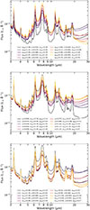 |
Fig. B.1. Synthetic mid-IR (3–30 μm) spectra demonstrating the influence of key dust parameters in the Draine et al. (2007) dust model. Each panel shows the variation of the spectrum by varying one parameter within its 95% confidence interval, while the rest are drawn independently from their assumed distributions. Top: Variation with the PAH mass fraction, qPAH. Middle: Variation with the fraction of dust mass exposed to high radiation fields, γ. Bottom: Variation with the minimum starlight intensity, Umin. We see that these three parameters have significant impact on the shape of the PAH spectrum when compared to that in Fig. B.2. All spectra have the same bolometric luminosity. |
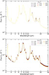 |
Fig. B.2. Synthetic mid-IR galaxy spectra (3-30 μm) highlighting the impact of ISM parameters. Top: Variation of the spectrum as a function of ionization parameter (log10U). Bottom: Variation with gas-phase metallicity (log10Z/Z⊙). Each line represents a mock galaxy spectrum generated with fixed ISM conditions while varying the labeled parameter. We see that the impact of these parameters on the shape of the PAH spectrum is subtle. All spectra have the same bolometric luminosity. |
All Tables
Description, range, probability distribution function, and reference of each physical parameter used to produce the simulated sample of galaxies.
Wavelength range (rest frame) and important features that describe our custom fixed photometric bands.
Comparison of the activity classification between our diagnostic and the 6.2 μm PAH EW classifier (EW6.2).
Classification results for a sample of real galaxies based on the diagnostic tailored for JWST/MIRI photometry.
All Figures
|
Fig. 1. Present-day SFRs against stellar mass for the DustPedia galaxy sample. The solid black line represents the MS of galaxies as defined by Elbaz et al. (2011), while the dashed black lines indicate the 1σ deviations from this sequence. Most of the galaxies lie along the MS, with only a few falling below it. |
| In the text | |
|
Fig. 2. Histograms indicating the shapes and ranges of the distributions of the SPS parameters (Table 1) used as input to the FSPS to produce our mock sample of galaxies. In the top row, from left to right, we show the distribution densities of metallicity (Z), the dust fraction exposed to a high ionization field (γ), and the ionization parameter of the gas (log10U), respectively. On the bottom row on the left, we show the minimum (average) ionization field of the ISM (Umin), while on the bottom right we see the fraction of dust in the form of PAH molecules (qPAH). Each parameter set contains these five parameters drawn randomly and independently from each other based on the probability distributions shown above. |
| In the text | |
|
Fig. 3. Color–color diagram of NUV − r against g − r comparing the distributions of the mock (black dots) and a real SDSS (red contours) galaxy sample. We see general agreement between the two galaxy samples for almost the entire range of these colors especially for (g − r) ∼ 0.6. Photometric bands from GALEX (NUV) and the SDSS survey (g and r). We also show a sample of photometrically selected passive galaxies (green contours) for comparison. The mock data were artificially augmented with noise to achieve an S/N of 10 to match to the selection criteria for the SDSS and GALEX bands. Contour levels denote the 10th, 25th, 50th, 75th, and 90th percentiles for each population. |
| In the text | |
|
Fig. 4. Color–color diagram of g − r against u − g comparing the distributions of a mock (black dots) and a real SDSS (red contours) galaxy sample. We see very good agreement between the two galaxy samples. Photometric bands from the SDSS survey are shown. We also show a sample of photometrically selected passive galaxies (green contours) for comparison. The mock data were artificially augmented with noise to achieve an S/N of 10 to match to the selection criteria for the SDSS bands. Contour levels denote the 10th, 25th, 50th, 75th, and 90th percentiles for each population. |
| In the text | |
|
Fig. 5. Color–color diagram of W1 − W2 against W2 − W3 comparing the distributions of a mock (black dots) and a real star-forming galaxies from SDSS (red contours). We see very good agreement between the two galaxy samples. Also, both samples occupy the area well bellow the W1 − W2 = 0.8 (dashed black line) demarcation line defined by Stern et al. (2012) between the AGN and non-AGN galaxies and the AGN selection wedge (solid black lines) defined by Mateos et al. (2012). We also show a sample of photometrically selected passive galaxies (green contours) for comparison. Photometric bands from the WISE survey are shown. The mock data were artificially augmented with noise to achieve an S/N of 10 to match to the selection criteria for the WISE bands. Contour levels denote the 10th, 25th, 50th, 75th, and 90th percentiles for each population. |
| In the text | |
|
Fig. 6. Mid-infrared (5–25 μm) spectrum of NGC 6120, observed with the IRS spectrograph aboard Spitzer, representing a typical star-forming galaxy (BPT class). In this spectrum, we mark the wavelength coverage of our four custom photometric bands, labeled in Table 2. The first three photometric bands (PAH1, PAH2, and PAH3) cover the strongest PAH emission features, while the last band (Cont215) covers a continuum region of the spectrum. |
| In the text | |
|
Fig. 7. Distributions of the three distinguishing features used to develop our diagnostic tool. From top to bottom: log10(PAH1/Cont215), log10(PAH2/Cont215), and log10(PAH3/Cont215), measured from both the S5 sample (green) of star-forming galaxies and our simulated sample of galaxies (purple). We find very good agreement between the two samples for all the features. |
| In the text | |
|
Fig. 8. Average mid-IR spectra of composite galaxies (based on the BPT optical diagnostics) classified as star-forming (SFG) and non-star-forming (NOT-SFG) based on our diagnostic. The composite galaxies predicted as star-forming galaxies (solid blue line) have similar average spectra with the typical MS star-forming galaxies (dashed black line). The composite galaxies predicted as not star-forming (solid blue line) have steeper spectra above 12 μm. The shaded area in both average spectra corresponds to the standard deviation of 1σ. |
| In the text | |
|
Fig. 9. Average mid-IR spectra of AGN galaxies (based on the BPT optical diagnostics) classified as star-forming (SFG) and non-star-forming (NOT-SFG) based on our diagnostic. The AGN galaxies predicted as star-forming galaxies (solid blue line) have similar average spectra with the normal star-forming galaxies (dashed black line). The AGN galaxies that have been predicted as not star-forming (solid blue line) have steeper spectra above 12 μm than the BPT-AGN predicted as star-forming galaxies. In addition, the average spectra of the AGN galaxies identified as non-star-forming exhibit clear emission lines of [Ne V] 14.3 μm (vertical dashed blue line) and [O IV] 25.9 μm (vertical dashed red line). These are tell-tale signs of a strong radiation field source. The shaded area in both average spectra corresponds to the standard deviation of 1σ. |
| In the text | |
|
Fig. 10. The [O IV] 25.9 μm/[Ne II] 12.8 μm ratio plotted against the EW of the 6.2 μm PAH feature for optically identified star-forming (blue stars), composite (black disks), and AGN (green squares) galaxies. The green lines represent the average AGN fractional contribution to a galaxy’s emission, based on the [O IV]/[Ne II] ratio (Sturm et al. 2002). The blue lines denote the average starburst fractional contribution determined from the EW of the 6.2 μm feature (Armus et al. 2007). The red circle highlights galaxies identified as star-forming based on our diagnostic tool. The uncertainties associated with each measurement are 1σ error. |
| In the text | |
|
Fig. 11. Recall score of our diagnostic as a function of redshift. The performance was recorded by training the algorithm using rest-frame spectra and testing the performance on the test sample of the redshifted simulated spectra at z= 0, 0.0125, 0.025, 0.05, 0.075, and 0.1. The scores are stable for up to z ∼ 0.02 and then drop smoothly. |
| In the text | |
|
Fig. 12. Star formation rate against stellar mass for galaxies from several galaxy samples (left panel). We correctly identify almost all the galaxies that fall in the area on the MS star-forming galaxies. As expected, we miss all the galaxies from samples that focus on BCDs and ULIRGs. The solid blue line shows the MS fit for star-forming galaxies from Elbaz et al. (2011), and the dashed blue lines are correspond to the 1σ error to this line. On the right panel, we plot the absolute magnitude in band W4 against the absolute magnitude in band W1 for the same galaxies. The former serves as a proxy of the star formation rate, while the latter as a proxy of the stellar mass of a galaxy. The star-forming galaxies identified correctly (blue circles) are clustered on the MS, while the star-forming galaxies missed tend to have higher MW4 values or correspond to extreme cases of galaxies (BCDs or ULIRGs). |
| In the text | |
|
Fig. 13. Color–color plot of W1 − W2 against the W2 − W3 for the same samples of galaxies introduced in Fig. 12. The normal star-forming galaxies we have identified correctly occupy the lower area of this plot, while extreme cases related to star formation (such as BCDs and ULIRGs) are scattered, exhibiting redder W1 − W2 and W2 − W3 colors. The dashed black lines delineate the optimal operational area of our diagnostic system. |
| In the text | |
|
Fig. A.1. Recall for star-forming galaxies, indicated by the green line, and contamination from AGNs, indicated by the red line. Both metrics were calculated on the observed sample (Sect. 2.1) as a function of the oneclassSVM nu parameter (i.e., population selection threshold). We observe that contamination begins to increase rapidly after nu = 0.9, marked by a horizontal blue line, which designates our selected value for nu. |
| In the text | |
|
Fig. B.1. Synthetic mid-IR (3–30 μm) spectra demonstrating the influence of key dust parameters in the Draine et al. (2007) dust model. Each panel shows the variation of the spectrum by varying one parameter within its 95% confidence interval, while the rest are drawn independently from their assumed distributions. Top: Variation with the PAH mass fraction, qPAH. Middle: Variation with the fraction of dust mass exposed to high radiation fields, γ. Bottom: Variation with the minimum starlight intensity, Umin. We see that these three parameters have significant impact on the shape of the PAH spectrum when compared to that in Fig. B.2. All spectra have the same bolometric luminosity. |
| In the text | |
|
Fig. B.2. Synthetic mid-IR galaxy spectra (3-30 μm) highlighting the impact of ISM parameters. Top: Variation of the spectrum as a function of ionization parameter (log10U). Bottom: Variation with gas-phase metallicity (log10Z/Z⊙). Each line represents a mock galaxy spectrum generated with fixed ISM conditions while varying the labeled parameter. We see that the impact of these parameters on the shape of the PAH spectrum is subtle. All spectra have the same bolometric luminosity. |
| In the text | |
Current usage metrics show cumulative count of Article Views (full-text article views including HTML views, PDF and ePub downloads, according to the available data) and Abstracts Views on Vision4Press platform.
Data correspond to usage on the plateform after 2015. The current usage metrics is available 48-96 hours after online publication and is updated daily on week days.
Initial download of the metrics may take a while.