| Issue |
A&A
Volume 703, November 2025
|
|
|---|---|---|
| Article Number | A86 | |
| Number of page(s) | 15 | |
| Section | Extragalactic astronomy | |
| DOI | https://doi.org/10.1051/0004-6361/202556035 | |
| Published online | 07 November 2025 | |
Realistic consecutive galaxy mergers form eccentric pulsar timing array sources
1
Dipartimento di Fisica “G. Occhialini”, Universitá degli Studi di Milano-Bicocca, Piazza della Scienza 3, I-20126 Milano, Italy
2
School of Mathematics and Physics, University of Surrey, Guildford GU2 7XH, UK
3
INAF – Osservatorio Astronomico di Brera, via Brera 20, I-20121 Milano, Italy
4
INFN, Sezione di Milano-Bicocca, Piazza della Scienza 3, I-20126 Milano, Italy
5
INAF – Osservatorio Astronomico di Padova, Vicolo dell’Osservatorio, 5, I-35122 Padova (PD), Italy
6
Astronomisches Rechen-Institut, Zentrum für Astronomie der Universität Heidelberg, Mönchhofstraße 12-14, 69120 Heidelberg, Germany
⋆ Corresponding author: This email address is being protected from spambots. You need JavaScript enabled to view it.
Received:
19
June
2025
Accepted:
23
August
2025
Abstract
Results from pulsar timing arrays (PTAs) show evidence of a gravitational wave background (GWB) consistent with a population of unresolved supermassive black hole binaries (BHBs). The observed spectrum shows a flattening at lower frequencies that can be explained by a population of eccentric BHBs. This study aims to determine the dynamical evolution and merger timescales of the most massive BHBs, which are potential sources of the GWB. We selected successive galactic major mergers from the IllustrisTNG100-1 cosmological simulation and re-simulated them at high resolution with the N-body code Griffin, down to binary separations of the order of a parsec. Coalescence timescales were estimated using a semi-analytical model that incorporates gravitational wave emission and stellar hardening. Throughout our investigation, we considered the impact of prior mergers on the remnant galaxy in the form of core scouring and anisotropy, which can influence the subsequent formation and evolution of BHBs. We find that all the binaries in our sample enter the PTA band with an eccentricity of e > 0.85: such a large eccentricity can impact the shape of the PTA observed GWB spectrum, and it highlights the importance of including the eccentricity of binaries when interpreting the PTA signal. Furthermore, we find that: (i) starting from initial separations of a few tens of kiloparsecs, the dynamical friction phase lasts for a few hundred million years; (ii) the binary formation time is not resolution-dependent; (iii) the scatter on the eccentricity at binary formation decreases with increasing resolution; and (iv) triple systems form whenever a third galaxy interacts with a binary that has not yet reached coalescence.
Key words: black hole physics / gravitational waves / methods: numerical / galaxies: interactions / galaxies: kinematics and dynamics / galaxies: nuclei
© The Authors 2025
 Open Access article, published by EDP Sciences, under the terms of the Creative Commons Attribution License (https://creativecommons.org/licenses/by/4.0), which permits unrestricted use, distribution, and reproduction in any medium, provided the original work is properly cited.
This article is published in open access under the Subscribe to Open model. This email address is being protected from spambots. You need JavaScript enabled to view it. to support open access publication.
1. Introduction
Supermassive black holes (BHs) are expected to reside at the centre of massive galaxies, with masses ranging between 106 − 1010 M⊙ (e.g. Kormendy & Richstone 1995; Kormendy & Ho 2013). The Λ cold dark matter (ΛCDM) theoretical model for galaxy evolution predicts that structures in the Universe form hierarchically. In this process, smaller systems develop first, followed by the formation of larger structures through accretion and subsequent mergers (Ostriker & Hausman 1977; White 1980; Lacey & Cole 1993). A natural result of these galactic encounters is the formation of BH pairs, whereby each BH resides in the merger remnant at a separation of the order of kiloparsecs from its companion (Barnes & Hernquist 1992). The dynamical evolution of the two BHs is governed by various physical processes that extract energy and angular momentum, drawing them towards the centre of the remnant, and potentially leading to their coalescence (Begelman et al. 1980).
The first mechanism that contributes to the slowing down of the BHs is dynamical friction against the stellar and dark matter (DM) content of the host galaxy (Chandrasekhar 1943). Dynamical friction ceases to be efficient when the velocity of the BHs becomes comparable with the velocity of the surrounding stars, and this occurs around the time the two BHs form a bound binary system, which typically happens at separations of about 100 pc for a 109 M⊙ binary.
From that point onwards, assuming a gas-poor environment, the binary shrinks (‘hardens’) due to three-body interactions with single stars: they eventually get ejected at high velocities, carrying away kinetic energy and thus increasing the binding energy of the black hole binary (BHB, Quinlan 1996; Sesana et al. 2006). This mechanism is expected to be efficient due to the triaxiality of the host’s potential that is induced by the merger process (Khan et al. 2016; Bortolas et al. 2018). In triaxial potentials, the total angular momentum of stars is not conserved along the orbit, allowing for a large population of stars on centrophilic orbits. These may pass arbitrarily close to the centre, where they can interact with the central BHB (e.g. Gualandris et al. 2017). Assuming that stellar hardening is capable of driving a ∼109 M⊙ BHB to a separation of the order of 1–0.1 pc on timescales shorter than a Hubble time, the physical process responsible for the final stages of binary evolution is gravitational wave (GW) emission, which can efficiently bring the system to coalescence (Peters 1964).
The superposition of the GW signals produced by a population of unresolved BHBs is expected to result in a GW background (GWB; Rajagopal & Romani 1995; Jaffe & Backer 2003; Sesana et al. 2008). The GWB can be observed via pulsar timing arrays (PTAs; Foster & Backer 1990) by searching for correlated deviations in the times of arrival (TOAs) of radio signals coming from millisecond pulsars. Pulsar timing arrays are mostly sensitive to low-redshift (z < 2), massive sources (M > 108 M⊙ with mass ratios of q > 1/4), which are expected to dominate the GWB signal (e.g. Sesana et al. 2008; Izquierdo-Villalba et al. 2022). In summer 2023, the European PTA (EPTA) and Indian PTA (InPTA), the North America Nanohertz Observatory for GWs (NANOGrav), the Parkes PTA (PPTA), and the Chinese PTA (CPTA) reported evidence of a correlated GWB, with a statistical significance of between 2-4 σ (EPTA Collaboration 2023a,b,c, 2024a,b; Smarra et al. 2023; Agazie et al. 2023a,b,c,d; Afzal et al. 2023; Reardon et al. 2023; Xu et al. 2023).
The amplitude of the GWB depends on the number of sources emitting GWs within the frequency range that PTAs are sensitive to (10−9 − 10−7 Hz). To be effective GW emitters, BHBs must achieve separations of the order of 1–0.1 pc (see above). For this reason, studying the timescales required for BHBs to reach this separation is essential for interpreting the GWB signal. Moreover, depending on the galactic environment and the efficiency of each physical process that drives the dynamical evolution of the binary, the lifetime of the BHB can exceed the time elapsing between a galactic merger and the subsequent one. As a result, systems including more than two BHs may form (e.g. Hoffman & Loeb 2007; Satheesh et al. 2025). According to Bell et al. (2006) and Lin et al. (2008), ∼30 − 70% of present-day spheroidal galaxies have experienced a major merger since z = 1. Thus, on average, all massive galaxies have undergone a merger in the last 10 Gyr, leading to ∼10% of BHBs possibly forming a triplet (assuming their lifetime to be ∼ 1 Gyr, Amaro-Seoane et al. 2010).
This paper has the main goal of simulating, for the first time, realistic consecutive major mergers of massive galaxies at low redshift, which can produce PTA sources. Starting from cosmological initial conditions, we accurately followed the dynamics of the BHBs thus formed using the state-of-the-art fast multiple method (FMM) code Griffin (Dehnen 2014), with the goal of determining the evolutionary timescales and the properties of these system, including the binary eccentricity and the probability of forming triplets.
The paper is structured as follows. In Section 2 we describe the methods, reporting (i) the selection criteria for merger trees in our chosen cosmological simulation (2.1), (ii) the method adopted to initialise the first merger of the tree (2.2), (iii) the precautions taken when initialising subsequent mergers (2.3), and (iv) the methods used to evolve the systems down to coalescence 2.4. We present our results in Section 3, discussing and comparing them with previous works. Finally, in Section 4 we draw our conclusions.
2. Methods
2.1. Selecting merger trees in IllustrisTNG100-1
IllustrisTNG100-1 (hereafter TNG100-1) is the highest-resolution cosmological, magneto-hydrodynamical simulation in the IllustrisTNG100 simulation suite (Springel et al. 2018; Pillepich et al. 2018; Nelson et al. 2018; Naiman et al. 2018; Marinacci et al. 2018). TNG100-1 simulates a cubic volume with side length of 110.7 Mpc, using AREPO (Springel 2010a), a moving, unstructured-mesh hydrodynamic code, with superposed smoothed-particle hydrodynamics gas particles (e.g. Springel 2010b). Star and DM particles have masses, respectively, of mbaryon = 1.4 × 10⁶ M⊙ and mDM = 7.5 × 10⁶ M⊙ and a softening length of ε = 0.74 kpc. The BHs are seeded with a mass of Mseed = 8 × 10⁵ h−1 M⊙ in halos with Mh ≥ 5 × 10¹⁰ h−1 M⊙. Their accretion follows the Bondi-Hoyle accretion model (Bondi & Hoyle 1944) capped at the Eddington limit; they are dynamically evolved, while their position is kept fixed at the potential minimum of the host galaxy.
All TNG100-1 data are stored in 99 snapshots, publicly available1. The merger history of the structures is easily reconstructable through the provided merger trees, built using the SubLink algorithm (Rodriguez-Gomez et al. 2015). In our work, we consider two galaxies to merge when they share the same SubLink descendant, and we define the merger snapshot as the snapshot of said descendant.
To choose our sample of subsequent mergers, we selected the last TNG100-1 snapshot (z = 0) and searched for galaxies with a stellar mass of M* ≥ 3 × 10¹¹ M⊙ (100 in total). Then we extracted their merger trees and we retained only the ones containing more than one major merger (q ≳ 1/4) at z < 2. This choice is motivated by the fact that the GWB signal is dominated by sources at low redshift (e.g. Sesana et al. 2008; Izquierdo-Villalba et al. 2022) and a high mass ratio. We obtained a total of five merger trees, containing two or three mergers each. The properties of the selected trees, i.e. (i) the redshift of the mergers, (ii) the BHs masses, (iii) the masses of the stellar and DM components of the progenitor galaxies, and (iv) the orbital parameters, are presented in Table 1.
Merger parameters.
2.2. Creating initial conditions for the first merger in the tree
We drew data relative to the progenitor galaxies of each encounter, choosing the TNG100-1 snapshot immediately before the merger2, and we then generated the initial conditions necessary to re-simulate the dynamical evolution of these mergers at high accuracy. Griffin is an FMM N-body code that allows one to control the (maximum) force errors directly and reliably, i.e. it does not generate an error distribution with a tail towards large force errors, as is otherwise typical for tree and/or FMM codes (Dehnen 2014).
We determined the eccentricity and pericentre of the orbit of the merging galaxies by treating them as a Keplerian two-body system. Since the DM halos may already be overlapping in the selected TNG100-1 snapshot, we considered an effective mass for the computation of the relative orbit, as is outlined in Sect. 2.3 of Fastidio et al. (2024). In agreement with our previous work, we find that the majority of the mergers in our sample have an extremely high initial eccentricity.
We re-modelled the merging galaxies, using the action-based galaxy modelling software AGAMA (Vasiliev 2019) to generate the initial conditions. Both the stellar bulge and the DM halo were generated by fitting a Hernquist profile (Hernquist 1990) to the density profiles in the TNG100-1 snapshot, including an exponential cut-off to match the profile truncation radius.
We initialised the primary galaxy with two different resolutions: N = 106 (low resolution, LR hereafter) and N = 2 × 10⁶ particles (high resolution, HR hereafter), allocating half of them to the DM halo and the remaining half to the stellar bulge. To improve the resolution in the central region of the galaxy, we employed the mass refinement scheme described in Attard et al. (2024). The scheme divides stellar and DM particles into four radial shells each, and oversamples particles in the inner zones at the expense of those in the external regions. The total number of particles was initially increased by up to a factor of 10, then the added particles were retained in the central shell, while the scheme progressively removed particles moving outwards, proportionally increasing the mass of the remaining ones. The total mass and density profile were thus preserved.
We determined the number of particles in the secondary galaxy so that: (i) their mass matched that of the particles in the primary galaxy, and (ii) the bulge-halo and primary-secondary mass ratios were maintained. The same mass refinement scheme was then applied to the secondary galaxy as well. To assess the resolution in the innermost part of our models, we calculated the number of particles within five times the influence radius of the primary BH3 (see Table 2), defined as the radius enclosing a mass in stars equal to twice the BH mass.
Resolution of our simulations.
Improving the resolution comes at the cost of increasing the mass ratio between the DM and stellar particles, which in general is not advisable, since it can lead to the segregation of artificially massive particles towards the centre. To mitigate this effect, we used individual softenings proportional to the particles mass (for both stellar and DM particles):
 (1)
(1)
where mstd is the particle mass and α is given by
 (2)
(2)
with ε0,std = 30 pc and mh, sh1 is the mass of halo particles in the innermost shell. Similarly, the softening length for BH-BH, BH-stars, and BH-DM interactions is
 (3)
(3)
where ε0,BH = 1 pc, mBH1 is the mass of the primary BH and mBH is the mass of the BH under consideration. After establishing stable models for both progenitors separately, we positioned them on the previously computed orbit, with an initial separation equal to the distance between the galactic centres in TNG100-1.
2.3. Creating initial conditions for the following mergers
When initialising the second (or third) merger within the same merger tree, it is important to take some additional precautions. There are two main scenarios to consider: (i) a sufficient amount of time has elapsed between the two mergers, resulting in a well-defined merger remnant and allowing the first BHB to merge; (ii) the time between consecutive mergers is so short that the third galaxy begins to interact with the first two before their merger is completed.
In the first scenario, we manually merged the two BHs when the binary separation reached the softening length ε0,BH. We then allowed the system to evolve in isolation until the time at which the second merger was flagged in TNG100-1. However, an inconsistency may arise between the mass of the remnant of the merger in Griffin and that of TNG100-1. In Griffin, the mass of the remnant is calculated as the sum of the masses of the two progenitors and remains constant over time. In contrast, masses in TNG100-1 evolve over time, which is typical of cosmological hydrodynamic simulations that allow for gas accretion onto the central BHs. Moreover, since galaxies do not evolve in isolation, they can interact with their environment, accrete material, and convert gas into stars. As a result, when initialising the second and third mergers, the mass of the primary galaxy (i.e. the merger remnant from the previous merger) in Griffin is usually lower than that in TNG100-1. We therefore adjusted the galaxy and BH masses to take growth into account, using the same procedure that is outlined in Sect. 2.2.
Because scouring in the first major merger carves a core in the stellar distribution, we set up subsequent mergers with a shallower density profile. In particular, we fitted the stellar and DM density profiles of the galaxy in Griffin with a Dehnen profile (Dehnen 1993) with central slope γ = 0.5. This has been shown to be consistent with core scouring profiles (e.g. Nasim et al. 2021). However, it is important to note that in this work we do not include natal kicks after coalescence, which can lead to the formation of flatter and larger cores, as is shown in Khonji et al. (2024). When initialising the galaxy with AGAMA, we set the masses of the galaxy components based on values drawn from TNG100-1, but distributed according to the density profiles thus obtained from Griffin.
Additionally, we computed the anisotropy parameter β from the Griffin’s last snapshot as
 (4)
(4)
where  ,
,  and
and  are the velocity dispersions in the three components of the spherical co-ordinates. We then plotted the radial anisotropy profile, excluding the regions where the number of particles is < 1000. The resulting profiles are typically nearly flat, with −0.29 < β < −0.24. We used this constant value of β in AGAMA to incorporate the anisotropy into the remnant model that we generated.
In the second scenario described above, in which the third galaxy begins to interact before the previous merger is complete, we considered the inclination angle between the trajectory of the new incoming galaxy and the orbital plane of the progenitors from the previous merger. In the snapshot before the new merger in TNG100-1, the previous merger has already formed a remnant. Note that the resolution of the cosmological simulation is significantly lower than that of the Griffin simulation. The third galaxy, on the other hand, is approaching along an orbit that can be defined as is outlined in Sect. 2.2, and whose total angular momentum can easily be calculated. We adopted the total angular momentum of the stellar component of the remnant galaxy in TNG100-1 (i.e. the primary progenitor of the new merger) as a good approximation for the total angular momentum of the orbit of the previous merger. We then computed the relative inclination from the two angular momenta and set up the inclination between the first and the second merger using this value.
2.4. Time evolution
For each merger tree, we initialised the first merger as described in Section 2.2 and evolved it using Griffin. We followed the evolution through the phases of dynamical friction, binary formation, and stellar hardening. We tracked the evolution of the relative separation between the BHs and calculated the Keplerian semi-major axis (a) and eccentricity (e) as a function of time.
Near the pericentre passages, the orbital parameters (particularly the eccentricity) can be quite noisy and poorly defined. We removed such passages by discarding points where the kinetic energy of the binary exceeds three times its potential energy.
After alternating between bound and unbound phases, the binary ultimately stabilises into a bound orbit. We define this moment as the time of binary formation (tb), i.e. when the Keplerian total energy4 remains negative.
We caution that our definition of the time of binary formation, tb, differs from that used in our previous work, in which it was empirically defined as the time at which the polynomial fit of the eccentricity evolution reached its minimum. The definition presented here has the key advantage of not relying on the existence of a clear minimum in the eccentricity data, which makes it more general.
We stopped the Griffin simulations when the BHB separation reached the softening length of the most massive BH (i.e. 1 pc), and we manually merged the BHs, placing a single BH with mass M = MBH, 1 + MBH, 2 in the centre of mass of the binary and assigning it the centre of mass velocity.
To reconstruct the final stages of the binary evolution (that cannot be reliably simulated with Griffin), we used a semi-analytical model (SAM). This model incorporates both the effects of stellar hardening (subscript ⋆) and GW emission (subscript GW), evolving the semi-major axis of the binary and its eccentricity using the following equations:
 (5)
(5)
 (6)
(6)
The rate of change of the orbital parameters due to stellar hardening is given by
 (7)
(7)
 (8)
(8)
with ρ and σ being, respectively, the stellar density and velocity dispersion within the radius of influence of the binary, and H and K the dimensionless hardening rate and eccentricity growth rate (Quinlan 1996). These depend on the binary’s mass ratio, eccentricity and separation and can be derived through three-body scattering experiments of the ejection of background stars by the BHB. Tabulated values given in Sesana et al. (2006) can be interpolated as required for specific merger configurations.
The rate of change due to GW emission, on the other hand, was obtained from Peters’ equations (Peters 1964):
 (9)
(9)
 (10)
(10)
where G is the gravitational constant, c is the speed of light in vacuum, M1 and M2 are the primary and secondary BH masses, respectively, and M is the total binary mass.
The initial conditions of the SAM (namely the initial values of a, ρ, and σ) were drawn directly from Griffin data: we selected a snapshot from the simulation at a time, t0,SAM, that satisfies the following criteria: (i) t0,SAM > tb, (ii) at t0,SAM, the mutual separation between the BHs is decreasing slowly (indicating that the binary system is already ‘hard’), and (iii) we have sufficient snapshots at t > t0,SAM to compare the evolution predicted by the SAM with the final part of the evolution observed in Griffin. The SAM was integrated using the Euler method, until one of the following criteria was met: (i) the binary merges or (ii) t > 1010 yr.
Our SAM admits three free parameters: the initial eccentricity5 (e0,SAM), α, and β, where the last two are normalisation parameters that can adjust the value of H and K, respectively, to account for more or less efficient stellar hardening, compared to the one obtained from scattering experiments. We then employed a Markov chain Monte Carlo (MCMC) sampler to compare the semi-analytical prediction with the evolution of a and e computed from Griffin data. We used uniform prior distributions and a Gaussian likelihood, defined as the root mean square of our data points with respect to the SAM. After computing the posteriors, the peak of the likelihood indicates the parameter values that best fit our data points. The time at which the SAM (run with the best-fit parameters) stops is defined as the time of binary coalescence.
To assess the uncertainty on the predicted coalescence time, we randomly extracted 100 samples from the posterior distributions of the parameters. We then used these samples to predict the corresponding coalescence times, which provide an estimate of the error in our predictions. When simulating the second and third merger of the trees, we applied the same methodology, the only difference being the initial condition settings (see Sect. 2.3).
3. Results and discussion
3.1. Evolutionary timescales
In Fig. 1 we present the merger tree 197109 – HR as an example of our results, and we plot the BH separation throughout the evolution (analogous figures for the other merger trees can be found in Appendix A).
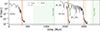 |
Fig. 1. Merger tree 197109 - HR. We show the time evolution of the BHs separation in Griffin simulations. The horizontal dashed black line indicates the softening length ε0,BH = 1 pc. Vertical red lines represent binary formation times; vertical yellow lines represent initial times chosen for the SAM; vertical green lines are the predicted coalescence times, with the corresponding uncertainties drawn as shaded green areas. Note that for the second BHB the predicted time of coalescence almost overlaps with t0,SAM. This is because the eccentricity at binary formation is so extreme that the system merges immediately due to GW emission. As a consequence, this particular system does not form a triplet. |
The first galactic merger begins with eccentricity e0 = 0.745 at a separation of d ∼ 15 kpc. This merger forms a bound BHB after ∼344 Myr (first red line). The binary is predicted to coalesce roughly 866 Myr after its formation (first green line), and around 163 Myr before the onset of the second merger.
The second and third galactic mergers, on the other hand, are separated by only ∼160 Myr, leading to the co-evolution of three different galaxies. The last galaxy is initialised with a smaller separation from the primary galaxy of the previous merger (∼4 kpc), compared to the ∼32 kpc separation between the two galaxies at the beginning of the second merger6. Due to the aforementioned small separation and the high orbital eccentricity (e0 = 0.997) of the last galactic merger, the last BH (BH4) forms a bound binary with the primary BH (BH1, 2) from the previous galactic encounter.
This second binary becomes bound ∼43 Myr after the onset of the last galactic merger (second red line), with an extremely high eccentricity (eb = 0.991). During the hardening phase, e increases further, reaching a value of 0.999 after roughly 27 Myr (second yellow line). Given the large mass of the BHB, the small separation, and the high eccentricity, its evolution is already GW-dominated at this point in time. Therefore, in this particular case, instead of using the SAM to infer the coalescence time, we employed the following equation:
 (11)
(11)
where Tc = a04/(4βe) is the predicted coalescence time for a circular binary, with βe = (64/5)(G3M1M2M)/c5 (Peters 1964). The predicted coalescence time is thus ∼28 Myr after binary formation (second green line). As a consequence, this particular system does not form a triplet. Finally, the remaining two BHs, i.e. the newly merged one (BH1, 2, 4) and the secondary BH coming from the second galactic encounter (BH3), become bound ∼364 Myr after the coalescence of the second binary (third red line), merging around 256 Myr after binary formation (third green line).
A summary of the binary formation and coalescence times for all the merger trees is provided in Table 3. Merger trees marked with an ‘x’ in the third BHB column are those that involve only two major mergers in TNG100-1. Some of the high-resolution simulations are particularly slow to run, and have not been completed; these are indicated in Table 3 with a ‘/’. We note, however, that their low-resolution counterparts do merge within a Hubble time, giving an indication of their evolutionary timescales. There are two exceptions among the LR runs: 17187-LR and 197109-LR. The third galactic merger of tree 17187 occurs immediately after the second, and all three galaxies involved have a similar separation, making it the slowest merger tree to simulate, even at low resolution (see Fig. A.1). In the 197109-LR simulation, on the other hand, the last two BHs (i.e. the remnant resulting from the coalescence of the second binary and the BH coming from the secondary galaxy of the second galactic merger) seem to stall in the LR run (see Fig. A.9), contrary to the behaviour observed in the HR version of the same tree (see Fig. 1). Finally, binaries that are marked with a (T) form before the coalescence of the previous BHB, thereby creating a triple system rather than a binary. For these systems, we have not included a coalescence time, as we plan to follow their evolution using the three-body integrator Galcode (Bonetti et al. 2016) (Fastidio et al., in preparation).
Simulations’ key times.
Considering that we have five merger trees, four of which completed in at least one of the two resolutions, our sample cannot capture the full statistics of merging binaries. However, we can highlight some important observations that may help us understand these results better and improve future studies: (i) Starting from an average separation of a few tens of kiloparsecs, the dynamical friction phase that causes the BHs to form a binary typically lasts for a few hundred million years, which is generally consistent with previous studies (e.g. Attard et al. 2024; Khonji et al. 2024). (ii) The binary formation times are mostly compatible between the LR and HR runs. (iii) Coalescence times tend to be shorter for HR runs, compared with their LR counterparts. This is generally due to a higher eccentricity at binary formation in the HR simulations (see Sect. 3.2). The first binary of 125027 represents an exception in this regard: the predicted coalescence time is shorter in the LR run, compared to the HR one; this is because, while the eccentricity at binary formation is roughly the same for both resolutions, in the LR simulation e increases more during the last phase of the N-body evolution, bringing the binary to coalescence earlier (see Figs. A.3 and A.4). However, it is important to notice that, while in the LR run we have enough data points after t0,SAM to see a clear rising trend in eccentricity, in the HR run the separation of the binary system is already close to ε0,BH when the SAM starts. As a result, there are only a limited number of data points available for the MCMC to calibrate the value of K (eccentricity growth rate), which makes the outcome sensitive to stochasticity. Nonetheless, the predicted time of coalescence in the HR run is less than twice as long, and this does not significantly affect the subsequent evolution of the tree. (iv) Three of the five merger trees form a triple BH system. Tree 168390 forms a triplet in both the high- and low-resolution runs. Trees 125028 and 197109, on the other hand, form a triplet only in the LR simulations. This outcome has implications for merger timescales and PTA signals, which will be discussed in our forthcoming paper. We caution that, while the best-fit coalescence time suggests the formation of triple BH systems, significant uncertainties, such as those in Tree 197109-LR, might cause the binary to merge prematurely, preventing tripletformation.
In Fig. 2, we show the dependence of the merger timescales on three parameters: (i) the initial distance between the two progenitor galaxies (d0); (ii) the initial orbital eccentricity of the galactic merger (e0); and (iii) the resolution of the simulation. The four panels illustrate the value of the dynamical friction timescale (ΔtDF = tb − t0, top panels), and the total coalescence time (Δtcoal = tcoal − t0, bottom panels) as a function of the initial separation between the progenitor galaxies. The data points are colour-coded according to the initial eccentricity of the galactic merger. In the left column, we show data drawn from the LR runs, while in the right we plot data from their HR counterparts. We notice a clear correlation between the initial separation and the dynamical friction timescale. However, for comparable d0 values, a higher eccentricity, e0, results in a shorter ΔtDF. There is, however, an exception to these general trends: in the upper right panel, we can see two points with roughly the same values of d0 and e0 (the two green diamonds), but with significantly different values of ΔtDF. These data points refer to the third BHB in the trees 1971097 (high ΔtDF value) and 125028 (low ΔtDF value). This inconsistency is likely due to the differences in masses and mass ratios of the two mergers, including both the BH, stellar, and DM components. The second system is generally more massive and has a higher mass ratio among all components of the primary and secondary progenitors, which accelerates the dynamical evolution. Finally, we note that the resolution of the simulations does not appear to affect ΔtDF, as the values of tb remain largely consistent between the LR and HR runs, as was previously mentioned.
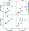 |
Fig. 2. For each BHB formed, we plot the dynamical friction timescale (ΔtDF = tb − t0, top panels), and the total coalescence time (Δtcoal = tcoal − t0, bottom panels) as a function of the initial distance between the progenitor galaxies (d0). Data are colour-coded according to the initial eccentricity of the galactic merger. Note that we chose to use log10(1 − e0) to make the colour gradient clearer, so the colour bar goes from high (yellow) to low (blue) eccentricity values. Panels on the left refer to LR runs, while panels on the right show data from their HR counterparts. Empty circles, squares, and diamonds represent the first, second, and third binary in each tree, respectively. |
The bottom panels depict a similar scenario regarding Δtcoal. Here, a higher e0 value does not necessarily lead to a shorter Δtcoal. This is because there is not a perfect correlation between e0 and eb (see Sect. 3.2) and the final part of the binary evolution (i.e. hardening and GW emission phases) can be much faster if eb is high. Moreover, there is a difference between LR and HR runs, whereby coalescence times are on average shorter for high-resolution simulations.
Lastly, we do not find any specific dependence of these timescales on the sequential nature of these mergers, with no significant differences observed between the first, second, and third BHBs formed (indicated by empty circles, squares, and diamonds, respectively). A longer evolutionary timescale might be expected in cored stellar profiles due to less efficient dynamical friction and hardening in a lower density environment. However, our chosen profiles for the second and third merger galaxies may not be sufficiently shallow to show this effect.
3.2. Eccentricity
One of the key parameters for determining merger timescales of BHBs is their eccentricity. Unfortunately, this parameter is also the most sensitive to stochastic effects caused by resolution (Nasim et al. 2020; Rawlings et al. 2023; Fastidio et al. 2024). In this section, we discuss the impact of eccentricity on our results and how it is affected by the resolution we have adopted.
Figure 3 shows the evolution of the Keplerian eccentricity of the three binaries formed in 197109-HR (the same simulation of Fig. 1). The first panel presents data referring to the first BHB. The galactic merger starts with a moderately high eccentricity (e0 = 0.745, cyan dot), while the resulting BHB forms with eb = 0.997 (red dot). During the hardening phase, e decreases slightly (at t = 370.7 Myr e = 0.990, orange dot), although the data show significant noise. This is why we opted to keep the initial eccentricity of our SAM as a free parameter, fitting it using an MCMC method, as mentioned in Sect. 2.4. The best fit value we find is eMCMC = 0.981, which is indeed somewhat lower.
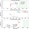 |
Fig. 3. Evolution of the orbital eccentricity of the first (top panel), second (middle panel), and third (bottom panel) BHBs formed in Tree 197109-HR. We highlight with vertical coloured lines the key times in the binary’s evolution: the initial time of the galactic merger (t0, cyan), time of binary formation (tb, red), time at which we start the SAM (tSAM, orange), time when the binary enters the PTA band (tPTA, blue), and time of coalescence (tcoal, green). For each time, we also report the corresponding eccentricity value, plotted as a point, following the same colour scheme. The horizontal orange line denotes the MCMC best-fit value of the initial eccentricity used for the semi-analytical evolution. |
Similarly, the second panel of Fig. 3 displays the evolution of the eccentricity of the second binary over time. It is important to note that this binary forms as a result of the third galactic merger. In this case, the primary BH is formed from the merger of the first binary, while the secondary BH is brought in from a fourth galaxy. The third galactic merger starts with e0 = 0.997, and the resulting BHB has a slightly lower but still significant eccentricity (eb = 0.991). After binary formation, the eccentricity approaches 1, reaching e = 0.999 at t = 1.60 Gyr. This high value means we cannot ignore GW emission, which drives the binary to coalescence.
Finally, the third panel shows data referring to the third BHB, formed when the remnant of the second binary and the BH from the secondary galaxy of the second galactic merger become bound. The second galactic merger starts with e0 = 0.986, while the formed binary has eb = 0.928, slightly lower than the original. Subsequently, e increases again, reaching e = 0.967 at t = 2.04 Gyr. This value is consistent with what we obtained from the MCMC fit. Analogous plots for the other merger trees can be found in Appendix A.
A summary of the eccentricity values at key times is presented in Table 4. We also report the SAM-predicted eccentricity upon entry in the PTA band (ePTA). As the reference for lowest frequency observable by PTA, we use fGW, p = 10−9 Hz, where fGW, p is the peak GW frequency, computed via
![Mathematical equation: $$ \begin{aligned} f_{\rm {GW,p}} = \frac{1}{\pi }\sqrt{\frac{GM}{[a(1-e^2)]^3}}(1+e)^{1.1954} ,\end{aligned} $$](/articles/aa/full_html/2025/11/aa56035-25/aa56035-25-eq27.gif) (12)
(12)
Key eccentricity values.
where M is the total mass of the binary (Wen 2003).
These values are provided only for binaries for which the data permit SAM predictions (eight in total). This includes binaries that do not form triple BH systems and those that were not evolved using Eq. 11. To define ePTA, we analysed the time evolution of the semi-major axis and orbital eccentricity obtained from the SAM. These parameters were then used to calculate fGW, p.
In Fig. 4 we illustrate the evolutionary tracks of the binaries formed in Tree 197109-HR8 within the eccentricity-fGW, p plane. When the systems enter the PTA band (shaded red area) at a reference frequency of 1 nHz, their orbital eccentricity is almost 1 (red cross). At this stage, they are not in the GW-dominated regime yet, and their eccentricity is still increasing because of stellar hardening. This occurs because these binaries are extremely eccentric; thus, the peak of their GW emission is shifted to higher frequencies compared to fGW = 2forb (where forb is their orbital frequency). As a consequence, these systems enter the PTA band sooner than their circular counterparts. To help the reader and guide the eye through the binary evolution in Fig. 4, we also plot the orbital frequency as a dashed line and we colour-code the tracks according to the time from t0,SAM to coalescence.
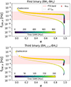 |
Fig. 4. Semi-analytical evolution of the first (top panel) and third (bottom panel) binary of tree 197109-HR in the fGW, p−eccentricity plane. The dashed grey line shows the evolution of the orbital frequency (forb), as a way to compare it with fGW, p. All the data points are colour-coded to indicate elapsed time (from t0,SAM = 0 to coalescence, for each binary). We use a red cross to highlight when the binaries enter the PTA band (shaded red area). |
The evolution of the semi-major axis and the eccentricity as a function of fGW, p of the whole sample of eight binaries for which we have a semi-analytical prediction is shown in Fig. 5, in which all appear to enter the PTA band (red shaded area) before the beginning of the circularisation phase. All binaries have an orbital eccentricity of e > 0.85 upon entry in the PTA band, as is highlighted in Fig. 6. This reinforces the importance of incorporating the eccentricity of binaries when analysing PTA data. A population of eccentric binaries is expected to flatten the GWB signal at lower frequencies, while boosting it at higher frequencies (e.g. Sesana 2015). Moreover, eccentric systems evolve faster, which may lead to an overall attenuation of the GWB across all frequencies (e.g. Chen et al. 2017; Kelley et al. 2017). Additionally, close pericentre passages may result in burst-like GW emissions that could be important when interpreting PTA data.
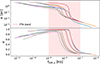 |
Fig. 5. Evolution of the semi-major axis (top panel) and the eccentricity (bottom panel) as a function of the peak GW frequency (fGW, p) of the eight binaries for which we have a semi-analytical prediction. The PTA band is represented as a shaded red area. |
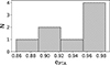 |
Fig. 6. Histogram of the eccentricity upon entry in the PTA band of all binaries for which we can compute the peak GW frequency (fGW, p). |
Following up on the results presented in Fastidio et al. (2024), we investigated the correlation between the initial eccentricity of the galactic merger (e0) and the eccentricity at binary formation (eb). We expected to find evidence of this correlation up to e0 ∼ 0.9 (see also Gualandris et al. 2022), while for larger values of e0 we anticipated a greater scatter in the results (σeb) that could lead to smaller eb values. According to Nasim et al. (2020), the stochastic effects responsible for the large σeb decrease as  , where N represents the number of particles used in the simulation. Rawlings et al. (2023), on the other hand, argue that this behaviour does not hold at extreme initial eccentricities, at which stochasticity becomes nearly inevitable and only weakly depends on resolution. As was mentioned, in this study we have a limited number of runs; thus, our goal is not to establish how the standard deviation, σeb, decreases (or not) with N (Gualandris et al., in preparation). Nevertheless, our HR results seem to favour a correlation between e0 and eb even for high eccentricities, with σeb = 0.13 with respect to the 1:1 correlation. On the other hand, in the LR runs, when the initial eccentricities are extremely high, eb tends to be lower and σeb = 0.30.
Figure 7 shows the difference (eb − e0) as a function of e0, where we include data from all binaries of our simulations. If there were a 1:1 correlation between eb and e0, the points should cluster along the horizontal line where (eb − e0) = 0. Generally, LR runs (empty dots) do not follow this trend: they tend to be more scattered than HR data, and in the region of high initial eccentricities (eb − e0) is always negative. In contrast, the HR runs (filled dots) on average produce binaries with higher eb, which are more consistent with the original merger eccentricity. For completeness, we also include data from Fastidio et al. (2024)9 (grey squares), which have a resolution comparable with our LR runs, and we generally find a good agreement.
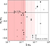 |
Fig. 7. Difference between the eccentricity at binary formation (eb) and the initial eccentricity of the merger (e0) as a function of the initial galactic merger orbital eccentricity (e0). The horizontal dashed line at (eb − e0) = 0 highlights where the points should be if there were a 1:1 correlation. Empty and filled dots represent data from the LR and HR runs, respectively. The shaded faint red area highlights the region where e0 > 0.9, while the shaded darker red area defines the region where e0 > 0.98. |
In Fig. 8, we plot the eccentricity at the time of binary formation as a function of e0. This includes all the binaries from our five merger trees. Different colours are used to distinguish between the first (red), second (blue), and third (green) binary in each tree, while empty and filled dots represent LR and HR runs, respectively. Similar to what is shown in Fig. 7, we observe that in the LR runs, when e0 > 0.9 (red shaded area), the value of eb tends to fall below the bisector (dashed line) and the scatter increases. However, there seems to be no significant impact on the correlation due to the sequential nature of these mergers; the first, second, and third binaries exhibit the same trend. In Appendix A, Fig. A.10, we show the same figure on a linear scale and we also include data from our previous work (Fastidio et al. 2024), to make the comparison easier.
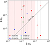 |
Fig. 8. Eccentricity at binary formation (eb) as a function of the initial galactic merger orbital eccentricity (e0). We use different colours to distinguish between data relative to the first (red), second (blue), or third (green) BHB of a tree. Empty and filled dots represent data from the LR and HR runs, respectively. The shaded red area highlights the region where e0 > 0.9. |
4. Conclusions
We searched for consecutive low-redshift major mergers in the cosmological simulation IllustrisTNG100-1, as these mergers lead to the formation of massive BHBs that are observable PTA sources. Our goal was to consistently re-simulate these systems at high resolution using the FMM code Griffin down to BH separations of the order of 1 pc. When initialising the second (or third) galactic merger of the selected merger trees, we accounted for both the effects of core scouring and anisotropy that can result from the preceding galactic merger, as these may influence subsequent mergers. We predicted the final stages of the BHBs’ evolution using a SAM that includes the effects of both stellar hardening and GW emission. We ran two versions of each simulation, changing their mass resolution, to compare results between the two. Our investigation centred on two primary aspects: the evolutionary timescales of the simulated systems and the evolution of the eccentricity of the formed BHBs. Our main findings are as follows:
-
The dynamical friction phase, which leads to BHs forming a binary, typically lasts for a few hundred million years, starting from an average separation of a few tens of kiloparsecs between the progenitor galaxies.
-
For comparable initial separations of the two galaxies at the onset of the galaxy merger, a higher initial eccentricity, e0, of the galaxy merger results in a shorter dynamical friction timescale, ΔtDF.
-
Binary formation times are mostly consistent between the LR and HR runs.
-
In all the finished runs, the BHBs merge within a Hubble time, making them observable PTA sources.
-
Coalescence times tend to be shorter for HR runs, compared with their LR counterparts. This is typically caused by a higher eccentricity at binary formation in the HR simulations.
-
The high-resolution runs seem to favour a correlation between e0 and eb (i.e. the eccentricity of the galaxy merger and the eccentricity of the binary at its formation) even for high eccentricities, with σeb = 0.13 with respect to the 1:1 correlation. On the other hand, the dispersion is larger in their LR counterparts (σeb = 0.30), since stochastic effects are stronger when the initial eccentricities are extremely high.
-
A larger σeb can result in a lower eccentricity at binary formation, and thus in longer coalescence times.
-
All the eight binaries for which we can compute the peak GW frequency (fGW, p) enter the PTA band with an orbital eccentricity of e > 0.85, indicating that eccentricity is a crucial parameter to include in PTA data analysis. This may explain or contribute to the flattening of the observed GWB signal.
Finally, three out of our five merger trees form a triple BH system: one was observed in both HR and LR runs, and two others were found only in the LR simulations. We shall present the results related to the three-body interactions of these systems in a follow-up paper, in which we shall track their dynamical evolution using the three-body integrator code Galcode to predict the GW emission that we can expect from such systems.
Note that, although we neglected the putative contribution of a gaseous component in the evolution of the BHBs, we expect our results to be robust against this assumption. In fact, our main focus is on PTA sources, which are extremely massive binaries hosted in massive galaxies (mostly ellipticals) at low redshift. Such systems are known for lacking a significant component of cold gas, which is also observationally reflected in the dramatic drop in luminous quasars at z < 1 (Hopkins et al. 2007). It is therefore unlikely that a massive BHB with M > 108 M⊙ in the low-redshift Universe is surrounded by a dense circumbinary cold gas disc that can significantly alter its dynamics. If this were the case, such a circumbinary disc would be self-gravitating (Franchini et al. 2022), a physical set-up that has been shown to promote binary shrinking while driving the binary eccentricity to relatively high values in the range of 0.5 < e < 0.8 (Franchini et al. 2024), contributing to the formation of eccentric BHBs.
Due to how the SubLink algorithm works, there are instances in which we cannot find both progenitor galaxies in the snapshot before the merger: in these cases, we followed the two back in time, until both were identified in the same snapshot.
This is computed on the initial conditions of the first merger of each merger tree, and used as a reference to compare our work with previous literature.
Note that when computing the total energy to define the time of binary formation, the data have already been cleaned to remove near pericentre passages.
We opted to keep e0 as a free parameter, contrary to what we did for a0, which is instead fixed as an initial condition. This choice is made because the scatter on the eccentricity evolution is usually much larger than the one on the semi-major axis, making it challenging to properly select an initial eccentricity value for the integration.
This depends solely on when each galactic merger is flagged in TNG100-1.
Note that this merger is not completed in its LR version, hence it is not present in the top left panel of Fig. 2.
Note that the second binary (BH1, 2-BH4) is not plotted since its coalescence time is computed using Eq. (11).
Note that the Keplerian eccentricity at the time of binary formation taken from Fastidio et al. (2024) has been re-calculated by applying the same method outlined in Sect. 2.4 to define when binary formation occurs.
Acknowledgments
AS acknowledges the financial support provided under the European Union’s H2020 ERC Consolidator Grant “Binary Massive Black Hole Astrophysics” (B Massive, Grant Agreement: 818691) and the European Union Advanced Grant “PINGU” (Grant Agreement: 101142079). AG would like to thank the Science and Technology Facilities Council (STFC) for support from grant ST/Y002385/1. The simulations were run on the Eureka2 HPC cluster at the University of Surrey.
References
- Afzal, A., Agazie, G., Anumarlapudi, A., et al. 2023, ApJ, 951, L11 [NASA ADS] [CrossRef] [Google Scholar]
- Agazie, G., Alam, M. F., Anumarlapudi, A., et al. 2023a, ApJ, 951, L9 [CrossRef] [Google Scholar]
- Agazie, G., Anumarlapudi, A., Archibald, A. M., et al. 2023b, ApJ, 951, L8 [NASA ADS] [CrossRef] [Google Scholar]
- Agazie, G., Anumarlapudi, A., Archibald, A. M., et al. 2023c, ApJ, 951, L50 [NASA ADS] [CrossRef] [Google Scholar]
- Agazie, G., Anumarlapudi, A., Archibald, A. M., et al. 2023d, ApJ, 951, L10 [CrossRef] [Google Scholar]
- Amaro-Seoane, P., Sesana, A., Hoffman, L., et al. 2010, MNRAS, 402, 2308 [NASA ADS] [CrossRef] [Google Scholar]
- Attard, K., Gualandris, A., Read, J. I., & Dehnen, W. 2024, MNRAS, 529, 2150 [Google Scholar]
- Barnes, J. E., & Hernquist, L. 1992, ARA&A, 30, 705 [Google Scholar]
- Begelman, M. C., Blandford, R. D., & Rees, M. J. 1980, Nature, 287, 307 [Google Scholar]
- Bell, E. F., Naab, T., McIntosh, D. H., et al. 2006, ApJ, 640, 241 [NASA ADS] [CrossRef] [Google Scholar]
- Bondi, H., & Hoyle, F. 1944, MNRAS, 104, 273 [Google Scholar]
- Bonetti, M., Haardt, F., Sesana, A., & Barausse, E. 2016, MNRAS, 461, 4419 [NASA ADS] [CrossRef] [Google Scholar]
- Bortolas, E., Gualandris, A., Dotti, M., & Read, J. I. 2018, MNRAS, 477, 2310 [Google Scholar]
- Chandrasekhar, S. 1943, ApJ, 97, 255 [Google Scholar]
- Chen, S., Sesana, A., & Del Pozzo, W. 2017, MNRAS, 470, 1738 [CrossRef] [Google Scholar]
- Dehnen, W. 1993, MNRAS, 265, 250 [NASA ADS] [CrossRef] [Google Scholar]
- Dehnen, W. 2014, Comput. Astrophys. Cosmol., 1, 1 [NASA ADS] [CrossRef] [Google Scholar]
- EPTA Collaboration, Antoniadis, J., Babak, S., et al. 2023a, A&A, 678, A48 [Google Scholar]
- EPTA Collaboration, InPTA Collaboration, Antoniadis, J., et al. 2023b, A&A, 678, A50 [CrossRef] [EDP Sciences] [Google Scholar]
- EPTA Collaboration, InPTA Collaboration, Antoniadis, J., et al. 2023c, A&A, 678, A49 [Google Scholar]
- EPTA Collaboration, InPTA Collaboration, Antoniadis, J., et al. 2024a, A&A, 685, A94 [NASA ADS] [CrossRef] [EDP Sciences] [Google Scholar]
- EPTA Collaboration, InPTA Collaboration, Antoniadis, J., et al. 2024b, A&A, 690, A118 [NASA ADS] [CrossRef] [EDP Sciences] [Google Scholar]
- Fastidio, F., Gualandris, A., Sesana, A., Bortolas, E., & Dehnen, W. 2024, MNRAS, 532, 295 [NASA ADS] [CrossRef] [Google Scholar]
- Foster, R. S., & Backer, D. C. 1990, ApJ, 361, 300 [NASA ADS] [CrossRef] [Google Scholar]
- Franchini, A., Lupi, A., & Sesana, A. 2022, ApJ, 929, L13 [NASA ADS] [CrossRef] [Google Scholar]
- Franchini, A., Prato, A., Longarini, C., & Sesana, A. 2024, A&A, 688, A174 [NASA ADS] [CrossRef] [EDP Sciences] [Google Scholar]
- Gualandris, A., Read, J. I., Dehnen, W., & Bortolas, E. 2017, MNRAS, 464, 2301 [Google Scholar]
- Gualandris, A., Khan, F. M., Bortolas, E., et al. 2022, MNRAS, 511, 4753 [NASA ADS] [CrossRef] [Google Scholar]
- Hernquist, L. 1990, ApJ, 356, 359 [Google Scholar]
- Hoffman, L., & Loeb, A. 2007, MNRAS, 377, 957 [NASA ADS] [CrossRef] [Google Scholar]
- Hopkins, P. F., Richards, G. T., & Hernquist, L. 2007, ApJ, 654, 731 [Google Scholar]
- Izquierdo-Villalba, D., Sesana, A., Bonoli, S., & Colpi, M. 2022, MNRAS, 509, 3488 [Google Scholar]
- Jaffe, A. H., & Backer, D. C. 2003, ApJ, 583, 616 [NASA ADS] [CrossRef] [Google Scholar]
- Kelley, L. Z., Blecha, L., Hernquist, L., Sesana, A., & Taylor, S. R. 2017, MNRAS, 471, 4508 [NASA ADS] [CrossRef] [Google Scholar]
- Khan, F. M., Fiacconi, D., Mayer, L., Berczik, P., & Just, A. 2016, ApJ, 828, 73 [Google Scholar]
- Khonji, N., Gualandris, A., Read, J. I., & Dehnen, W. 2024, ApJ, 974, 204 [NASA ADS] [CrossRef] [Google Scholar]
- Kormendy, J., & Ho, L. C. 2013, ARA&A, 51, 511 [Google Scholar]
- Kormendy, J., & Richstone, D. 1995, ARA&A, 33, 581 [Google Scholar]
- Lacey, C., & Cole, S. 1993, MNRAS, 262, 627 [NASA ADS] [CrossRef] [Google Scholar]
- Lin, L., Patton, D. R., Koo, D. C., et al. 2008, ApJ, 681, 232 [Google Scholar]
- Marinacci, F., Vogelsberger, M., Pakmor, R., et al. 2018, MNRAS, 480, 5113 [NASA ADS] [Google Scholar]
- Naiman, J. P., Pillepich, A., Springel, V., et al. 2018, MNRAS, 477, 1206 [Google Scholar]
- Nasim, I., Gualandris, A., Read, J., et al. 2020, MNRAS, 497, 739 [Google Scholar]
- Nasim, I. T., Gualandris, A., Read, J. I., et al. 2021, MNRAS, 502, 4794 [NASA ADS] [CrossRef] [Google Scholar]
- Nelson, D., Pillepich, A., Springel, V., et al. 2018, MNRAS, 475, 624 [Google Scholar]
- Ostriker, J. P., & Hausman, M. A. 1977, ApJ, 217, L125 [Google Scholar]
- Peters, P. C. 1964, Phys. Rev., 136, 1224 [Google Scholar]
- Pillepich, A., Nelson, D., Hernquist, L., et al. 2018, MNRAS, 475, 648 [Google Scholar]
- Quinlan, G. D. 1996, New A, 1, 35 [NASA ADS] [CrossRef] [Google Scholar]
- Rajagopal, M., & Romani, R. W. 1995, ApJ, 446, 543 [NASA ADS] [CrossRef] [Google Scholar]
- Rawlings, A., Mannerkoski, M., Johansson, P. H., & Naab, T. 2023, MNRAS, 526, 2688 [NASA ADS] [CrossRef] [Google Scholar]
- Reardon, D. J., Zic, A., Shannon, R. M., et al. 2023, ApJ, 951, L6 [NASA ADS] [CrossRef] [Google Scholar]
- Rodriguez-Gomez, V., Genel, S., Vogelsberger, M., et al. 2015, MNRAS, 449, 49 [Google Scholar]
- Satheesh, P., Blecha, L., & Kelley, L. Z. 2025, arXiv e-prints [arXiv:2506.04369] [Google Scholar]
- Sesana, A. 2015, in Gravitational Wave Astrophysics, Astrophys. Space Sci. Proc., 40, 147 [Google Scholar]
- Sesana, A., Haardt, F., & Madau, P. 2006, ApJ, 651, 392 [Google Scholar]
- Sesana, A., Vecchio, A., & Colacino, C. N. 2008, MNRAS, 390, 192 [NASA ADS] [CrossRef] [Google Scholar]
- Smarra, C., Goncharov, B., Barausse, E., et al. 2023, Phys. Rev. Lett., 131, 171001 [NASA ADS] [CrossRef] [Google Scholar]
- Springel, V. 2010a, MNRAS, 401, 791 [Google Scholar]
- Springel, V. 2010b, ARA&A, 48, 391 [NASA ADS] [CrossRef] [Google Scholar]
- Springel, V., Pakmor, R., Pillepich, A., et al. 2018, MNRAS, 475, 676 [Google Scholar]
- Vasiliev, E. 2019, MNRAS, 482, 1525 [Google Scholar]
- Wen, L. 2003, ApJ, 598, 419 [NASA ADS] [CrossRef] [Google Scholar]
- White, S. D. M. 1980, MNRAS, 191, 1P [Google Scholar]
- Xu, H., Chen, S., Guo, Y., et al. 2023, Res. Astron. Astrophys., 23, 075024 [CrossRef] [Google Scholar]
Appendix A: Additional plots
Here we show analogous plots to Fig. 1 and Fig. 3 for all the other merger trees, both in their LR and HR versions and point out peculiarities of each one. The colour scheme and the legends are the same used for Fig. 1 and Fig. 3, unless otherwise stated. Note that (i) the eccentricity upon entry in the PTA band is plotted only for binaries for which fGW, p can be computed (i.e. they do not form triplets and their later evolution is predicted using the SAM model); (ii) when the coalescence time of a binary is computed using Eq. 11 we do not plot any uncertainty on it; (iii) in this paper we do not report the coalescence time of triple BH systems.
Fig. A.1 shows results that refer to the merger tree 17187-LR. In panel (a) one can see that the second and third galactic mergers occur a few billion years after the first, both at very low redshifts (z = 0.21 and z = 0.17). When the third galactic merger is initialised, the three galaxies involved are roughly at the same separation of a few tens of kiloparsecs. This makes the simulation quite slow to form a potential second and third BHB (or triple system). Only data relative to the first BHB eccentricity are thus available and shown in panel (b). Moreover, due to the low redshift of this encounter, there is a high chance that it will not result in a bound BH system within a Hubble time. In Fig. A.2 we present the same merger tree as Fig. A.1, but in its high-resolution version. Note that the HR runs are generally slower since more computationally expensive and here it results in a lack of data relative to the third galactic merger.
In panel (a) of Fig. A.3, showing the time evolution of the BHs separation of merger tree 125027-LR, we can see an example of complete two-merger tree, while the high-resolution version has yet to form the second bound BHB (see Fig. A.4).
Fig. A.5 shows one of the complete three-merger trees that also forms a triple BH system in its low-resolution version (tree 125028-LR). We note that the first BHB forms between BH1 (coming from the primary galaxy of the first galactic merger) and BH3 (from the secondary galaxy of the second galactic merger). This is because (i) the initial separation between galaxy 1 and galaxy 3 is smaller than the separation between galaxy 1 and galaxy 2 and (ii) BH1 and BH3 are more massive than BH2, making the dynamical friction more efficient on them. In panel (a) we can see that the time of coalescence of the first BHB is predicted to be after the binary formation time of the second BHB, thus forming a triple system. We do not plot the initial SAM time and coalescence time of the second BHB, since we will follow the evolution of this triple system with the three-body integrator Galcode and present our results in F. Fastidio et al. (in preparation). When looking at the eccentricity evolution in panel (b), note that: (i) the initial eccentricity e0 plotted in the "First BHB" panel is the eccentricity of the second galactic merger (since the involved BHs are BH1 and BH3), (ii) the value of e0 in the "Second BHB" panel is the orbital eccentricity of the first galactic merger (for the same reason). The HR version of this tree, shown in Fig. A.6, does not form a triple BH system, because the first BHB (BH1 and BH3, like in the LR version) forms with an extremely high eccentricity and coalesces faster due to GW emission (tcoal is predicted via Eq. 11).
In Fig. A.7 and Fig. A.8 we show data that refer to merger tree 168390, in its LR and HR versions, respectively. This complete two-merger tree forms a triple BH system in both resolution runs. Like in tree 125028, the third galaxy is initialised at a separation that is smaller than the separation between the primary and secondary galaxy of the first merger, leading BH3 to be involved in the formation of the first binary. Differently from tree 125028, however, BH3 binds with BH2, but the explanation is analogous: BH2 and BH3 are more massive than BH1. In panel (a) of Fig. A.8 we see that in the HR run the three BHs undergo multiple close encounters before the inner BHB merges, while this is not the case in the low-resolution version.
Finally, in Fig. A.9 we report data relative to the low-resolution version of tree 197109, the one used as example in the main body of the paper. We note that in this LR run, the first BHB forms with an eccentricity that remains almost constant in the last stages of the Griffin evolution. This leads to a small MCMC best-fit value of K (the parameter that refers to the eccentricity growth rate) and thus a long (and uncertain) coalescence time. As a result, the first BHB in this LR version is predicted to coalesce after the formation of the second binary, thus forming a triple BH system.
Fig. A.10 shows the correlation between the initial eccentricity of the galactic mergers and the eccentricity at binary formation, similar to Fig. 8. This plot is presented on a linear scale, and we have included data from Fastidio et al. (2024) (empty black squares) to facilitate comparison.
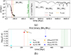 |
Fig. A.1. (a) Merger tree 17187-LR: time evolution of the BHs separation in Griffin simulations. The horizontal dashed black line indicates the softening of BHs particles in our simulation. Vertical coloured lines highlight key evolutionary times: initial galactic merger time (cyan), time of binary formation (red), time when we start the SAM (orange), and time of coalescence (green). The shaded green area represents the error on the predicted coalescence time, while the grey area denotes a jump in time of 7.2 × 10³ Myr, used to make the plot clearer. (b) Evolution of the orbital eccentricity of the first BHB (BH1 and BH2) formed in Tree 17187-LR. Vertical lines are coloured according to the same colour scheme as in panel (a). The vertical blue line shows when the binary is predicted to enter the PTA band by the SAM. For each key time, we plot the value of the orbital eccentricity with a point of the corresponding colour. The horizontal orange line denotes the MCMC best-fit value of the initial eccentricity used for the semi-analytical evolution. |
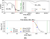 |
Fig. A.2. (a) Merger tree 17187-HR: time evolution of the BHs separation. The plotted grey area denotes a jump in time of 7.6 × 10³ Myr, used to make the plot clearer. (b) Evolution of the orbital eccentricity of the first BHB (BH1 and BH2) formed in Tree 17187-HR. |
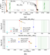 |
Fig. A.3. (a) Merger tree 125027-LR: time evolution of the BHs separation. (b) Evolution of the orbital eccentricity of the first (BH1 and BH2) and second (BH1, 2 and BH3) binary formed in Tree 125027-LR. |
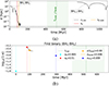 |
Fig. A.4. (a) Merger tree 125027-HR: time evolution of the BHs separation. (b) Evolution of the orbital eccentricity of the first BHB (BH1 and BH2) formed in Tree 125027-HR. |
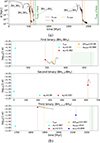 |
Fig. A.5. (a) Merger tree 125028-LR: time evolution of the BHs separation. (b) Evolution of the orbital eccentricity of the first (BH1 and BH3), second (BH1, 3 and BH2, triplet) and third (BH1, 3, 2 and BH4) binary formed in Tree 125028-LR. |
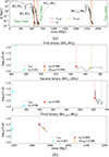 |
Fig. A.6. (a) Merger tree 125028-HR: time evolution of the BHs separation. (b) Evolution of the orbital eccentricity of the first (BH1 and BH3), second (BH1, 3 and BH2) and third (BH1, 3, 2 and BH4) binary formed in Tree 125028-HR. |
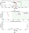 |
Fig. A.7. (a) Merger tree 168390-LR: time evolution of the BHs separation. (b) Evolution of the orbital eccentricity of the first (BH2 and BH3) and second (BH2, 3 and BH1, triplet) binary formed in Tree 168390-LR. |
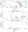 |
Fig. A.8. (a) Merger tree 168390-HR: time evolution of the BHs separation. (b) Evolution of the orbital eccentricity of the first (BH2 and BH3) and second (BH2, 3 and BH1, triplet) binary formed in Tree 168390-HR. |
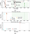 |
Fig. A.9. (a) Merger tree 197109-LR: time evolution of the BHs separation. (b) Evolution of the orbital eccentricity of the first (BH1 and BH2), second (BH1, 2 and BH3, triplet) and third (BH1, 2, 3 and BH4) binary formed in Tree 197109-LR. |
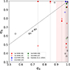 |
Fig. A.10. Eccentricity at binary formation (eb) as a function of the initial galactic merger orbital eccentricity (e0). We use different colours to distinguish between data relative to the first (red), the second (blue) or the third (green) BHB of a tree. Empty and filled dots represent data from the LR and HR runs, respectively. The empty black squares are data from our previous work (Fastidio et al. 2024), whose resolution is comparable to our LR runs. The shaded red area highlights the region where e0 > 0.9 |
All Tables
All Figures
|
Fig. 1. Merger tree 197109 - HR. We show the time evolution of the BHs separation in Griffin simulations. The horizontal dashed black line indicates the softening length ε0,BH = 1 pc. Vertical red lines represent binary formation times; vertical yellow lines represent initial times chosen for the SAM; vertical green lines are the predicted coalescence times, with the corresponding uncertainties drawn as shaded green areas. Note that for the second BHB the predicted time of coalescence almost overlaps with t0,SAM. This is because the eccentricity at binary formation is so extreme that the system merges immediately due to GW emission. As a consequence, this particular system does not form a triplet. |
| In the text | |
|
Fig. 2. For each BHB formed, we plot the dynamical friction timescale (ΔtDF = tb − t0, top panels), and the total coalescence time (Δtcoal = tcoal − t0, bottom panels) as a function of the initial distance between the progenitor galaxies (d0). Data are colour-coded according to the initial eccentricity of the galactic merger. Note that we chose to use log10(1 − e0) to make the colour gradient clearer, so the colour bar goes from high (yellow) to low (blue) eccentricity values. Panels on the left refer to LR runs, while panels on the right show data from their HR counterparts. Empty circles, squares, and diamonds represent the first, second, and third binary in each tree, respectively. |
| In the text | |
|
Fig. 3. Evolution of the orbital eccentricity of the first (top panel), second (middle panel), and third (bottom panel) BHBs formed in Tree 197109-HR. We highlight with vertical coloured lines the key times in the binary’s evolution: the initial time of the galactic merger (t0, cyan), time of binary formation (tb, red), time at which we start the SAM (tSAM, orange), time when the binary enters the PTA band (tPTA, blue), and time of coalescence (tcoal, green). For each time, we also report the corresponding eccentricity value, plotted as a point, following the same colour scheme. The horizontal orange line denotes the MCMC best-fit value of the initial eccentricity used for the semi-analytical evolution. |
| In the text | |
|
Fig. 4. Semi-analytical evolution of the first (top panel) and third (bottom panel) binary of tree 197109-HR in the fGW, p−eccentricity plane. The dashed grey line shows the evolution of the orbital frequency (forb), as a way to compare it with fGW, p. All the data points are colour-coded to indicate elapsed time (from t0,SAM = 0 to coalescence, for each binary). We use a red cross to highlight when the binaries enter the PTA band (shaded red area). |
| In the text | |
|
Fig. 5. Evolution of the semi-major axis (top panel) and the eccentricity (bottom panel) as a function of the peak GW frequency (fGW, p) of the eight binaries for which we have a semi-analytical prediction. The PTA band is represented as a shaded red area. |
| In the text | |
|
Fig. 6. Histogram of the eccentricity upon entry in the PTA band of all binaries for which we can compute the peak GW frequency (fGW, p). |
| In the text | |
|
Fig. 7. Difference between the eccentricity at binary formation (eb) and the initial eccentricity of the merger (e0) as a function of the initial galactic merger orbital eccentricity (e0). The horizontal dashed line at (eb − e0) = 0 highlights where the points should be if there were a 1:1 correlation. Empty and filled dots represent data from the LR and HR runs, respectively. The shaded faint red area highlights the region where e0 > 0.9, while the shaded darker red area defines the region where e0 > 0.98. |
| In the text | |
|
Fig. 8. Eccentricity at binary formation (eb) as a function of the initial galactic merger orbital eccentricity (e0). We use different colours to distinguish between data relative to the first (red), second (blue), or third (green) BHB of a tree. Empty and filled dots represent data from the LR and HR runs, respectively. The shaded red area highlights the region where e0 > 0.9. |
| In the text | |
|
Fig. A.1. (a) Merger tree 17187-LR: time evolution of the BHs separation in Griffin simulations. The horizontal dashed black line indicates the softening of BHs particles in our simulation. Vertical coloured lines highlight key evolutionary times: initial galactic merger time (cyan), time of binary formation (red), time when we start the SAM (orange), and time of coalescence (green). The shaded green area represents the error on the predicted coalescence time, while the grey area denotes a jump in time of 7.2 × 10³ Myr, used to make the plot clearer. (b) Evolution of the orbital eccentricity of the first BHB (BH1 and BH2) formed in Tree 17187-LR. Vertical lines are coloured according to the same colour scheme as in panel (a). The vertical blue line shows when the binary is predicted to enter the PTA band by the SAM. For each key time, we plot the value of the orbital eccentricity with a point of the corresponding colour. The horizontal orange line denotes the MCMC best-fit value of the initial eccentricity used for the semi-analytical evolution. |
| In the text | |
|
Fig. A.2. (a) Merger tree 17187-HR: time evolution of the BHs separation. The plotted grey area denotes a jump in time of 7.6 × 10³ Myr, used to make the plot clearer. (b) Evolution of the orbital eccentricity of the first BHB (BH1 and BH2) formed in Tree 17187-HR. |
| In the text | |
|
Fig. A.3. (a) Merger tree 125027-LR: time evolution of the BHs separation. (b) Evolution of the orbital eccentricity of the first (BH1 and BH2) and second (BH1, 2 and BH3) binary formed in Tree 125027-LR. |
| In the text | |
|
Fig. A.4. (a) Merger tree 125027-HR: time evolution of the BHs separation. (b) Evolution of the orbital eccentricity of the first BHB (BH1 and BH2) formed in Tree 125027-HR. |
| In the text | |
|
Fig. A.5. (a) Merger tree 125028-LR: time evolution of the BHs separation. (b) Evolution of the orbital eccentricity of the first (BH1 and BH3), second (BH1, 3 and BH2, triplet) and third (BH1, 3, 2 and BH4) binary formed in Tree 125028-LR. |
| In the text | |
|
Fig. A.6. (a) Merger tree 125028-HR: time evolution of the BHs separation. (b) Evolution of the orbital eccentricity of the first (BH1 and BH3), second (BH1, 3 and BH2) and third (BH1, 3, 2 and BH4) binary formed in Tree 125028-HR. |
| In the text | |
|
Fig. A.7. (a) Merger tree 168390-LR: time evolution of the BHs separation. (b) Evolution of the orbital eccentricity of the first (BH2 and BH3) and second (BH2, 3 and BH1, triplet) binary formed in Tree 168390-LR. |
| In the text | |
|
Fig. A.8. (a) Merger tree 168390-HR: time evolution of the BHs separation. (b) Evolution of the orbital eccentricity of the first (BH2 and BH3) and second (BH2, 3 and BH1, triplet) binary formed in Tree 168390-HR. |
| In the text | |
|
Fig. A.9. (a) Merger tree 197109-LR: time evolution of the BHs separation. (b) Evolution of the orbital eccentricity of the first (BH1 and BH2), second (BH1, 2 and BH3, triplet) and third (BH1, 2, 3 and BH4) binary formed in Tree 197109-LR. |
| In the text | |
|
Fig. A.10. Eccentricity at binary formation (eb) as a function of the initial galactic merger orbital eccentricity (e0). We use different colours to distinguish between data relative to the first (red), the second (blue) or the third (green) BHB of a tree. Empty and filled dots represent data from the LR and HR runs, respectively. The empty black squares are data from our previous work (Fastidio et al. 2024), whose resolution is comparable to our LR runs. The shaded red area highlights the region where e0 > 0.9 |
| In the text | |
Current usage metrics show cumulative count of Article Views (full-text article views including HTML views, PDF and ePub downloads, according to the available data) and Abstracts Views on Vision4Press platform.
Data correspond to usage on the plateform after 2015. The current usage metrics is available 48-96 hours after online publication and is updated daily on week days.
Initial download of the metrics may take a while.